event study analysis: comparison of mergers and

1

Empirical Findings of Mergers and Acquisitions in

the European Electricity and Gas Industry after the

5th

Wave

Supervisor: Prof. dr. A.H.F. Verboven

Student: Huiting Fu

Student Number: s996797

Study Program: International Management Master Program-Finance track

Tilburg University, March 15, 2011

2

Abstract

In this thesis, I research the phenomenon of the M&A raised after the 5th wave in European

electricity and gas industry. I want to find out what the results are after mergers and acquisitions

among European firms in electricity and gas industry. Moreover, this research expands its

investigation by searching the relevant factors affecting the bidder companies‟ valuation change.

The data collected for the research is from the bidder‟s takeover premium. The main tasks of this

research are (1) to use the event study analysis and statistical method to observe the influence to

the valuation change of the bidder companies after the 5th merger wave; (2) to implement the

linear regression analysis to find out the factors affecting the cumulative abnormal returns around

the M&A event time (CAR) after the 5th wave.

3

Contents

Chapter 1 Introduction ...................................................................................................................... 5

1.1 Introduction ............................................................................................................................. 5

1.2 Research questions .................................................................................................................. 5

1.3 Methodology ........................................................................................................................... 5

1.4 Structure of the thesis .............................................................................................................. 6

Chapter 2 Literature Review ............................................................................................................. 7

2.1 Review of M&A activity development (6 waves) ................................................................... 7

2.2 Classification of M&A ............................................................................................................ 9

2.3 Specific characteristics of the M&A in electricity and gas sector ......................................... 10

2.3.1 Restructuring .................................................................................................................. 12

2.3.2 Competition .................................................................................................................... 13

2.3.3 Regulation ...................................................................................................................... 14

2.3.4 Privatization ................................................................................................................... 15

Chapter 3 The Opportunities and Barriers of the M&A after the 5th Wave .................................... 16

3.1 Opportunities ......................................................................................................................... 16

3.2 Problem and barriers ............................................................................................................. 18

3.3 Research questions and hypothesis ....................................................................................... 19

Chapter 4 Data and Methodology ................................................................................................... 22

4.1 Data collection ...................................................................................................................... 22

4.1.1 Collecting the data of the bidder companies .................................................................. 22

4.1.2 Collecting the data of the stock price of the bidder companies ...................................... 23

4.2 Research methodologies – Event Study ................................................................................ 24

4.2.1 Identify the event ........................................................................................................... 24

4.2.2 Calculate the normal returns .......................................................................................... 25

4.2.3 Calculate and analyze the abnormal returns ................................................................... 26

4.3 Research methodologies – Regression Analysis ................................................................... 29

4.3.1 Observed factors ............................................................................................................ 29

4.3.2 To formulate the relationship between CAR and the factors .......................................... 30

4.3.3 Regression Analysis by SPSS ........................................................................................ 31

Chapter 5 Summary and Conclusions ............................................................................................. 41

5.1 Literature review, opportunities and barriers ........................................................................ 41

4

5.2 Event Study ........................................................................................................................... 41

5.3 Regression Analysis .............................................................................................................. 43

5.4 Conclusions ........................................................................................................................... 45

REFERENCE .................................................................................................................................. 46

5

Chapter 1 Introduction

1.1 Introduction

Currently, restructuring in electricity and gas sector in European countries is a hot

issue. The first merger and acquisition occurred in this area in Europe is in the United

Kingdom in 1989, and the change was driven by the large differences in electricity

tariffs across regions [8]. Recently, there are a lot of opportunities of investments in

power industry in many European countries provided by the governments. These

investments used to be only state-owned monopolies, but the ongoing restructuring

moves away the monopolies and brings more competence.

So far, after the 5th

wave (see section 2.1 for the definition), many major European

energy companies, such as E.ON and RWE, have announced that Eastern Europe will

be their next target where they will expand towards. This phenomenon indicates that

not only the Western Europe has consolidated to the point where the number of the

potential acquisition target is reduced, but also that Central Europe is a better fit for

their current long-term strategies [9]. Moreover, this trend is likely to accelerate in the

near future. Therefore, studying the M&A activities in the European energy area and

its influence is an interesting subject.

1.2 Research questions

My thesis will study what the effects of the mergers and acquisitions among the

European companies in electricity and gas industry are after the 5th

wave, and I focus

on two of the sub-questions:

(1) Is the value of the observed bidder companies in European electricity and gas

industry significantly affected by the mergers and acquisitions?

(2) What would be the main factors that affect the valuation change of the bidder

companies and what the strength of the influence by these factors are?

1.3 Methodology

In my thesis, I will use event analysis to study the first research question. This method

– event study, has been introduced in Tilburg University as the lecture note for the

course Empirical Finance and Investment Cases by Frank de Jong [1]. Event study is

an important tool in finance. When a significant event happened on a company (such

as M&A in our case), it is difficult to measure the valuation change of a company. In

6

empirical finance, the impact of the significant event can be measured by the change

in the stock price of the company around the event time. The measuring approach is

based on the statistical tests of the abnormal returns. For more details about the event

study methodology, see chapter 4 in this thesis.

Assuming that there is a valuation change of the companies influenced by the M&A

activities, then what factors would actually influence the valuation change? I will use

regression analysis to study the second research question. Regression Analysis is,

based on collecting massive observed data, using statistical method to formulate a

regression relationship function between the dependent variable and the independent

variables [31]. If the function contains only one independent variable, then the

regression analysis is called simple regression analysis; if the function contains

multiple independent variables, it is called multiple regression analysis. In my thesis, I

will observe three factors, so I will use multiple regression analysis.

1.4 Structure of the thesis

The remainder of this thesis is structured as the following. The next chapter is

literature review, from the overview of the process of M&A in Europe to the

classification of merger and acquisition. Besides, specific characteristics of the M&A

in electricity and gas sector will be illustrated. In chapter 3, I will focus on the

discussion about the opportunities and the barriers to the M&A activities after the 5th

wave, explaining the main trend of the activities and the positive factors that affected

the mergers and acquisitions in the electricity and gas sector as well as the negative

factors. In the fourth chapter, the data sampling procedure and the research

methodology will be demonstrated and explained. With the collected data, I will

perform the event study and the regression analysis. In chapter 5, I will state the

research conclusion, as well as what the further research questions of my thesis would

be.

7

Chapter 2 Literature Review

Extensive researches have verified that mergers and acquisitions (M&A) come in

waves. Currently, the world is experiencing the 6th

wave. In my thesis I will study the

impact after the 5th

wave which takes place mainly in Europe and the US [10]. The

changes occurred after the 5th

wave has made a huge impact in many industries,

including the power area in Europe. My research focuses on finding out the impact of

the mergers and acquisitions among the European companies in electricity and gas

industry after the 5th

wave, and I will first introduce the M&A wave history in the

following section.

2.1 Review of M&A activity development (6 waves)

Waves are defined as a phenomenon that the activities occur in bursts interspersed

with relative inactivity [11]. Although this description is not enough to acknowledge

precisely a “wave”, but up until now there is no accurate definition or exact

measurement to capture wave phenomenon that is widely accepted. There are still a

small number of researchers who research on recognizing or measuring the M&A

waves. Authors use direct observation to examine bursts on the M&A patterns as a

“consensus” on their M&A related studies. Cools and van de Laar [12] present an

overall picture of depicting the consequence of the M&A waves which is showed in

Figure 1 M&A Waves Overview.

Figure 1 M&A Waves Overview

As you can see from Figure 1 M&A Waves Overview, the M&A waves since 1897, based

on the number of mergers, are executed with different levels of peaks and troughs. So

8

far, there have been six waves indicated and examined where most of the observations

took place in the US since it has run a long way of the M&A. Then it is followed by

UK and recently by Continental Europe.

The First Wave (1893 to 1904): The first wave happened in the US in a period of

economic expansion following a decade of stagnation. A particular characteristic of

the first wave is the horizontal merger performed by the giant companies. During that

time, this kind of merger has a name of horizontal consolidation. The wave during this

time is described as merger for monopoly.

The Second wave (1919 to 1929): The second wave also occurred in the US and it

was accompanied by significant economic growth and stock market boom. The wave

is mainly held by oligopolistic structure purpose by the large enterprises. This wave

was ended because of the 1929 Crash and the Great Depression.

The Third Wave (1955 to 1969-1973): This wave experienced the concept of

conglomeration which took hold of US companies‟ management. The scale of all the

mergers was not large. Some of them were relatively large acquires but they were

unrelated mergers with purpose of achieving growth through diversification. However,

companies could not get the expected benefits from the diversification under the

crashed conglomerate stocks.

UK has much longer history for M&A activities compared to any other European

countries started from 1960s since it has several similarities in terms of company

structures, characteristics and regulations to the US. This wave occurred in the UK is

characterized by horizontal merger followed by some signs of conglomerate merger in

the latter years. This is different from the US M&A movements in the same period,

however, the movements in the UK had somewhat triggered M&A movements in

Europe.

The Fourth Wave (1974-1980 to 1989): The fourth wave includes acquisitions and

divestitures. Many US companies made simultaneously acquisitions and divestitures

to expand the competitive advantage and to exit those which would limit their

competitive advantage. The wave is characterized by many developments like junk

bonds, hostile takeovers, financing and steadily increasing volume and size of LBOs.

Along this wave, UK had the same characteristics as in the US. Continental Europe

had been affected by the move also. Although there is no certainty, some literature

points out that the M&A activities in continental Europe have increased since 1984

with much smaller size and volume.

The Fifth Wave (1993-2000): This wave started in the US area. During this wave,

unprecedented size companies were created on the assumption that size does matter.

9

High stock price simultaneously affected the companies to keep conducting deals to

maintain their competition level. Another dramatic characteristic is the global view of

competition to create distinguished competitive advantage which led to the growth of

the size and volume of the cross border takeovers.

This pattern of movements affected not only the US but also the European countries.

Compared to the US, the number and the size of the deals in the continental Europe

have raised greatly with the reason of the increasing number of intra-European

countries deals and the stability of transatlantic deals. At the same time, euro currency

has a big impact on the wave because it reduces currency risk and home bias

investments.

The Sixth Wave (2002-2010): This wave is introduced by Martin Lipton [13], who

believes the new merger activities which has increased from 1.2 billion US$ in 2002

to 3.4 billion US$ by the end of 2006. He pointed out that the most typical features of

the wave were government support, globalization factors, low-interest financing,

hedge fund and the growth of private equity funds.

Although there is no direct evidence to show the sixth wave is global, the M&A

activities occurred in many markets in the world, especially in the European markets.

Some researchers believe that the fifth wave is actually the first international wave

because of the fast growing cross-border takeover in that period [14]. The increasing

number of hostile takeovers, which prefers immediate acquisitions rather than the

changes of the structure of capital markets, is caused by the stability of economic

conditions and management strategy [15].

2.2 Classification of M&A

There are several ways in which a firm can be acquired by another firm.

Merger and Consolidation

In a merger the target firm is absorbed by the acquiring firm, and becomes part of the

acquiring firm. After the merger, the target firm ceases to exist as a separate business

entity. Consolidation is very similar to merger. However, the difference between

merger and consolidation is that in a consolidation, both the acquiring firm and the

acquired firm terminate their previous legal existence and a new firm will be created

by both the target and bidding firm. In a word, merger and consolidation result in

combinations of the assets and liabilities of acquired and acquiring firms.

Acquisition of Stock

An acquisition, also known as a takeover, is the buying of one company (the „target‟)

by another. An acquisition may be friendly or hostile. Acquisition of stock is the way

10

to purchase the firm‟s voting stock in exchange for cash, shares of stock, or other

securities. Sometimes the acquisitions are finished by the private offer between the

managements of one firm and the other. Sometimes, it can also be used by a tender

offer. In a tender offer a firm offers to buy the outstanding stock of another firm at a

specific price publicly. The offer is communicated to the target firm‟s shareholders by

public announcements such as newspaper advertisements and mailings to

stockholders. When the acquirer takes an offer directly to the firm‟s management or

its board of directors, it is called friendly tender offer. However, if the acquirer

approaches the shareholders of the firm directly with a tender offer for their shares, it

becomes hostile tender offer. Hostile takeovers are not very popular, for its higher

transaction costs.

Acquisition of Assets

It is the kind of acquisition that the bidder company purchases the assets of the target

company. In the course of the acquisition, the bidder can buy the assets they want and

leave the assets and liabilities they don‟t want. After that, the assets of the target firm

are transferred to the acquiring firm and the target firm remains as an empty shell

company. The shareholders of the target firms can get the cash from the acquisition by

dividends or through liquidation. The legal process of transferring assets can be

costly.

2.3 Specific characteristics of the M&A in electricity and gas sector

The new M&A especially the liberalization initiatives in Europe and elsewhere began

in the early 1990s because of the reduced political concern over energy supply

security. The ending of the cold war made importing gas from Russia less risky in an

environment where liberalization favored the building of new gas-fired plants [16].

European reform was pursued at two parallel levels [16]. First, under the EU

Electricity Market Directives, member countries were required to take at least a

minimum set of steps by certain key dates toward the liberalization of their national

markets. Second, the European Commission promoted efforts to improve the

interfaces between national markets by improving cross-border trading rules, and to

expand cross-border transmission links. Trading rules are being developed with

industry agreement and the EU has subsidized some cross-border transmission link

upgrades.

The first and second EU Electricity Market Directives of 1996 and 2003 focused on

unbundling the industry and on a gradual opening of national markets. The second

directive further promotes competition by toughening regulation of access to networks

and requiring independent regulators. Regulations of cross-border trade aims to

facilitate market integration (Table 1 EU Electricity Directives). The second directive

11

aims to achieve

(1) unbundling of Transmission System Operators (TSOs) and Distribution

System Operators (DSOs) from the rest of the industry;

(2) free entry to generation;

(3) monitoring of supply competition;

(4) full market opening;

(5) promotion of renewable sources;

(6) strengthening the role of the regulator;

(7) a single European market.

In EU countries, raising the standards of regulation came rather late, which was after

the market structure and rules had been established. Thus in Italy and Spain,

regulators are weak in the face of established incumbent company interests. In

mid-2005, despite of the full liberalization of the German electricity market, there was

no central energy regulators yet established1

. Also, privatizing state-owned

monopolies has not been part of the EU- wide drive toward liberalization of the

industry. Therefore the requirements of regulation and other different type of the

reforms become imminent. The M&A in the gas and electricity industry has several

distinguishing features which will be illustrated in the following paragraphs.

Table 1 EU Electricity Directives

1 The regulator for telecommunications and post will also assume responsibility for electricity and gas. The new

regulatory authority (REGIP) is pending, for the enactment of the new energy law (ENWG) in 2005.

12

2.3.1 Restructuring

Restructuring is the corporate management term which refers to the changes of the

companies‟ structure in order to make the companies more profitable and better

organized. One of the popular restructuring methods is separation. An effective

separation of transmission system operators from generation is important for effective

wholesale competition, because it is beneficial for network competitions. Therefore

more and more companies are involved in the vertical separation evolution.

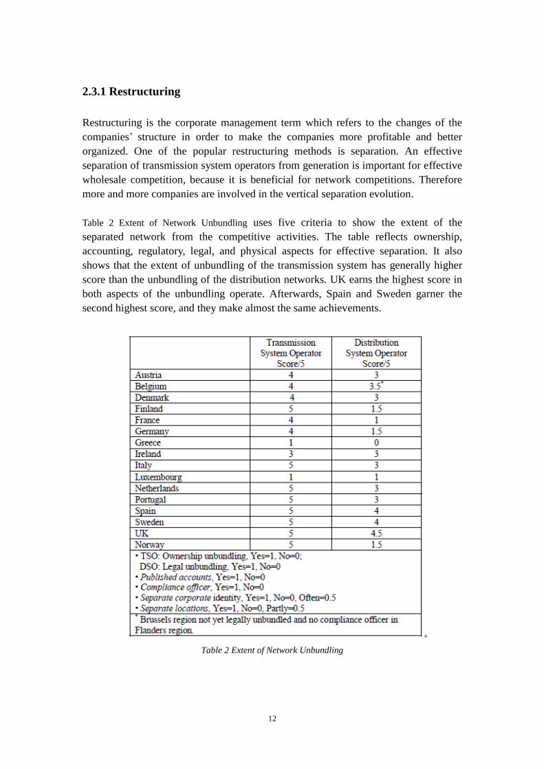
Table 2 Extent of Network Unbundling uses five criteria to show the extent of the

separated network from the competitive activities. The table reflects ownership,

accounting, regulatory, legal, and physical aspects for effective separation. It also

shows that the extent of unbundling of the transmission system has generally higher

score than the unbundling of the distribution networks. UK earns the highest score in

both aspects of the unbundling operate. Afterwards, Spain and Sweden garner the

second highest score, and they make almost the same achievements.

Table 2 Extent of Network Unbundling

13

2.3.2 Competition

In European countries, many countries already enter in the generation of complete

competition, and all large users and small consumers can freely choose their own

suppliers [16]. Moreover for the aspect of the distribution utilities, the 2003

Electricity Directive issued that it was not anymore allowed for the single-buyer

model to operate the distribution networks. This restriction has already been adopted

by Northern Ireland, Portugal and Italy. In addition, the standards of the competition

required the third-party access to the distribution networks.

In European electricity market, most of the countries, at least in principle, are now

open to competition. Although there is no requirement announced by the directives,

some countries have already extended market opening to households. Figure 2 Actual

and Expected Levels of Market Opening (by units sold) shows the description of the levels

of market opening from 1995 to 2004 in European electricity area. From the chart in

the figure we can see there is mounting growth from 1995 to 1999 and the extent

gradually enlarged afterwards. The actual market opening exceeded much more than

the expected estimation. So based on the results already achieved, the 2003 Directive

required that all non-household customers could freely choose their electricity

supplier by 1 July 2004, followed by full market opening to all household customers

by 1 July 2007.

Figure 2 Actual and Expected Levels of Market Opening (by units sold)

14

2.3.3 Regulation

Appropriate regulation especially implementing regulated third-party access to

distribution networks is rather important for effective competition. Recognizing the

importance of this, the 2003 Electricity Directive required member countries to

establish independent regulatory agencies. Genoud and Finger [16] observed that a

degree of convergence in European electricity regulation with the European

Commission is an influential factor to the independent regulatory agencies. Gilardi

[19] made a comparative analysis of the independent regulatory agencies in the EU,

and concluded the results that electricity industry had varied levels of the agencies

and could be more and more independent in the future.

Besides, incentive–based regulation of the distribution networks could make the

natural monopoly segment of the industry more efficient and cost saving. Figure 3

Estimated Breakdowns of Expected Electricity Prices in 2004 shows the difference of final

price of the electricity paid by the end-users in member countries in 2004. The figure

indicates that Germany has the highest transmission and distribution charges due to

the absence of incentive-based schemes. However, Norway and UK which are the

countries with longest incentive-based regulation of networks have the lowest charges

of distribution and transmission. The UK also indicates the lowest retail supply

margin.

Figure 3 Estimated Breakdowns of Expected Electricity Prices in 2004

(50 MWh/year Customer, euro/MWh before Taxes)

15

2.3.4 Privatization

EU electricity Directives do not make much effort on the need for private ownership

[16]. The most extensive privatization programs have taken place in the UK and

Portugal, and Italy has undertaken partial privatization. France although has not yet

processed the privatization, it is believed there was possibility in the near future. In

the Netherland the transmission and distribution utilities remained in public

ownership until 2005 [20]. The Nordic countries - Norway, Sweden, and Finland -

gradually introduced an open international market in electricity during the 1990s. In

addition, the EU electricity Directives introduced a new electricity law in 1998 which

requires member states to open their electricity markets for international trading. The

introducing of the new law was due to such a limitation that member states could

require all electricity for public consumption to be sold through a 'single buyer'.

At the early stage of implementing the privatization, by means of splitting large

companies to increase competition is easy and effective. In the Netherlands and

Norway, this method has another effect that avoids the possibility of national

companies falling into the other foreign companies‟ hands. As the time goes by, there

should be more and more countries getting used to the privatization which breaks

down the monopoly situation in the power industry.

16

Chapter 3 The Opportunities and Barriers of the M&A after the

5th Wave

Prior to the 5th

wave, the thinking of the mergers and acquisitions of the electricity

and gas industry is mainly about the public reform, and the business among the

countries. However, requirements on the private distribution and transmission of the

electricity and gas industry could not be neglected any more. More and more

European countries begin to realize that these requirements are not dangerous and

impossible, but affordable and operational. Alongside, there still exists some

difficulties and barriers to the revolution which also needs to pay attention to.

3.1 Opportunities

In the theory of microeconomic it is suggested that competition and the profit

motivation result in internal (production) and external (market) efficiency and that the

benefits are passed on to customers and the economy in the form of lower prices and

costs. The Electricity Supply Industry (ESI) has important physical characteristics that

shape its optimal regulatory design. It involves (1) large sunk costs which limit entry

possibilities, (2) vertical stages (generation, transmission, distribution and retailing) of

production with different optimal scales, and (3) non-storable goods need to be

delivered through an instantaneous balance of supply and demand at all nodes. M&A

activities bring the competitors more chances to achieve the efficiency, and also the

customers more benefits.

M&A especially the form of liberalization in the ESI needs creation of the

combination of competitive energy and retail markets. Besides, regulated transmission

and distribution activities are important as well. Successful liberalization requires

well-organized energy, associated supporting services and transmission capacity

markets. These requirements help the competitors to achieve competition much more

effective and operational.

Electricity liberalization around the world could produce a measure of consensus over

some common measures for achieving a well functioning market-oriented industry.

Liberalization generally requires implementation of one or more of the following

inter-related steps: sector restructuring, introduction of competition in wholesale

generation and retail supply, incentive regulation of transmission and distribution

networks, establishing an independent regulator, and privatization [21] [22] described

in Table 3 Main Measurements in Electricity Reform.

17

Table 3 Main Measurements in Electricity Reform outlines the measures for reforming a

vertically integrated and publicly owned ESI into a competitive and privately owned

industry. In practice, the actual measurement should consider both the specific aspects

of the national electricity and gas industry and the general features of the

liberalization model.

Table 3 Main Measurements in Electricity Reform [21] [22]

The aim of vertical unbundling is to separate potentially competitive generation and

supply from the natural monopoly activities of transmission and distribution networks.

The aim of horizontal separation is to create enough effective competition in

generation and retailing where economies of scale favor competition. In some

situation competition and /or efficiency may be promoted by increased horizontal

concentration in retailing or distribution. This may be the case where large numbers of

small distribution companies sell electricity (as was the case in the Netherlands until

relatively 2005) [23].

Restructuring also includes horizontal splitting of the involved generation firms or

merging of retailing firms. These restructuring activities aim to change market

concentration to theoretically and empirically competitive levels (usually there should

be more than 5 effective competitors in a market). Besides, in order to accelerate

competition in generation in the short run and encourage new entry in the long-run, it

is essential to prevent high levels of concentration in the existing markets. In the

long-run, new entry in generation and supply, and interconnections with other systems

can also increase competition in the market. Slow growth and excess capacity in many

European electricity and gas markets limit profitable entry opportunities for

newcomers, and continuing high levels of concentration in generation and retail

markets limit competition [24].

18

To establish the competitive markets structure requires government initiative. All

examples of successful restructuring (England and Wales, Norway) illustrate the

essential of the regulation published by the government to facilitate competition.

Regulation can be very good at policing a competitive system [25]. Moreover on the

regulation measurement, accessing the regulated third-party has proven the most

effective and widely used approach to the provision of network access [25].

Regulation also takes into account for the charges of distribution and transmission.

Normally the price should be one third of the final electricity or gas prices. In addition,

there is significant potential for efficiency improvement and cost savings in European

networks both within and between countries, because the average cost inefficiency of

the orders is 40% until 2003 in the European electricity and gas industry [26].

Another measurement is about the ownership. Many reforming countries have sold off

public enterprises or allowed new private entry. The main effect of privatization is

that the pursuit of profit by private owners will lead to efficiency improvement and

cost saving [27]. An increase in the ownership diversity can also accelerate direct

competition in the generation and supply activities and formulate regulation of

networks by comparative performance. In addition, privatization could make some

benefits for the government, which could help to reduce the government‟s liabilities in

the future [28].

In some countries (notably the UK, but also the Netherlands and Spain) the resulting

restructuring was accompanied by privatization, in others, such as Germany, private

ownership was already common, while yet others retained public ownership (notably

France) or partial privatization (Italy). Reasons for this were that privatization put a

considerable number of new companies into playing on the stock market. The second

reason is that the electricity demand is growing slowly, so organic growth2 is slow,

leaving profits either to be returned to shareholders or spent on acquisitions.

Therefore there is more and more privatization generated within the public owned

companies in the industry.

3.2 Problem and barriers

In contrast to the United States, mergers between energy companies in Europe have

been subject to rather relaxed standards, and consequently many mergers have been

allowed to proceed, which would cause economists considerable disquiet.

In EU, It seems poorly equipped to either assess or prevent problem caused by the

mergers. Mergers between mainly domestic energy companies are left to national

2 Organic growth: in finance, organic growth is the process of business expansion due to increased output, sales,

or both.

19

competition authorities, even when they have significant impacts on other member

states. There is a famous case about the E.On-Ruhrgas merger, which was condemned

by the German Monopoly Commission but approved by the German government.

However, the merger did not fall under the jurisdiction of the European Commission,

although German plays very important role in transmission route in EU and E.On

controls interconnectors into neighbor states.

Although, there is a tendency that the new restructuring will be a trend, several

findings cited that there are still be some problems which restricted the new type of

restructuring. One of the most obvious difficulties of the restructuring of the industry

is the special character which is the industry normally being controlled by the public

and restructured between the countries, and the personal companies not often being

mentioned [17]. Another doubt is whether the personal companies‟ joint will make the

efficiency affect the whole industry [17]. Last but not the least, the specific energy

laws in EU and every EU countries are the major barriers to the new reforms.

The other limitation confronting the Commission is the tension between the

longer-run objective of creating integrated and competitive energy markets, and the

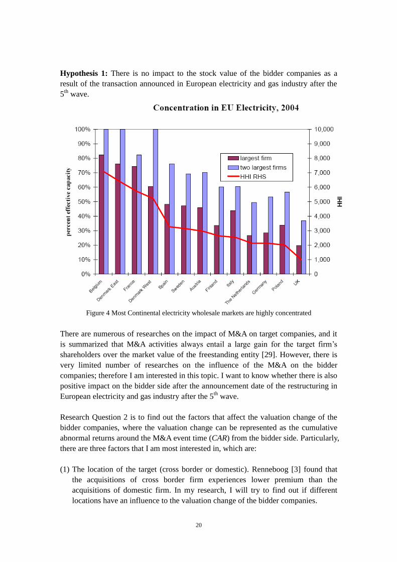
short-run test of the impact of a merger. Figure 4 Most Continental electricity wholesale

markets are highly concentrated3 shows the description of the concentration in EU

electricity industry. From the figure we can see there is an obvious concentration

already formulated in the industry. To break down the concentration and formulate

better competition market seems not easy and crucial.

3.3 Research questions and hypothesis

Based on the former analysis, this research will generate two questions about the

situation of the M&A in European electricity and gas industry.

(1) Is the stock value of the observed bidder companies in European electricity and

gas industry significantly affected by the mergers and acquisitions?



To solve the first research question I will set up a hypothesis and use event study to

research (either approves or rejects the hypothesis to give a final conclusion). For the

second research question, I will first set up a model function to formulate the

relationship between the valuation change of the bidder companies and the affecting

factors, and then use regression analysis to quantify the strength of the effects by the

factors.

3 HHI is the Herfindah1 Hirschman Index, the sum of the squared percentage market shares. The measures may

under or overstate market power as they ignore capacity tightness and import options.

20

Hypothesis 1: There is no impact to the stock value of the bidder companies as a

result of the transaction announced in European electricity and gas industry after the

5th

wave.

Figure 4 Most Continental electricity wholesale markets are highly concentrated

There are numerous of researches on the impact of M&A on target companies, and it

is summarized that M&A activities always entail a large gain for the target firm‟s

shareholders over the market value of the freestanding entity [29]. However, there is

very limited number of researches on the influence of the M&A on the bidder

companies; therefore I am interested in this topic. I want to know whether there is also

positive impact on the bidder side after the announcement date of the restructuring in

European electricity and gas industry after the 5th

wave.

Research Question 2 is to find out the factors that affect the valuation change of the

bidder companies, where the valuation change can be represented as the cumulative

abnormal returns around the M&A event time (CAR) from the bidder side. Particularly,

there are three factors that I am most interested in, which are:

(1) The location of the target (cross border or domestic). Renneboog [3] found that

the acquisitions of cross border firm experiences lower premium than the

acquisitions of domestic firm. In my research, I will try to find out if different

locations have an influence to the valuation change of the bidder companies.

21

(2) The technique of acquisition (privatization or other forms). New restructuring

based on privatization is an important discussion in the study, so I want to

research whether the M&A following privatization has an obvious influence on

the valuation change of the bidder companies.

(3) The method of payment (pay by cash or other payment methods). Renneboog [3]

reported that the bidder‟s shareholders favored cash payment more than equity

payment because the equity payment pattern declines more than the ones by cash

payment. In this research, I will try to find out whether the payment has a

significant influence to the valuation change of the bidder companies.

To research the relationship between the three factors and valuation change of the

bidder companies, I will first set up a model function to formulate the relationship,

and then use regression analysis to quantify the strength of the effect by every factor.

For more details refer to chapter 4.

22

Chapter 4 Data and Methodology

The first research question is whether the mergers and acquisitions affecting the value

of the observed companies in European electricity and gas industry. However, it is not

easy to measure how much the valuation of a company has been changed after a

certain event occurred to the company. One of the common-used methods in corporate

finance and investment analysis is to measure the change in the stock price around the

time when the event decision becomes public message [1]. Hereafter I refer this

approach as the Event Study, which is to use the abnormal stock returns round the

event date to carry out some statistical tests. In section 4.2, I will give an introduction

in more details to my event study methodology.

The second research question is to find out the main factors that affect the valuation

change of the bidder companies. The most interesting factors I want to observe are the

location of the target (domestic or abroad), if the acquisition technique is privatization,

and if the method of the payment is by cash. The most common method to study the

relationship between the independent variables and the dependent variable is

regression analysis. I assume it to be a linear regression, and I will use SPSS as the

tool to perform the analysis.

4.1 Data collection

To conduct my event study, the data collection is composed of two parts:

(1) Collecting the information (the factors to be observed) of the bidder companies of

the mergers and acquisitions;

(2) Collecting the stock price of these companies around the time of mergers and

acquisitions announcement.

4.1.1 Collecting the data of the bidder companies

In this thesis I only study the stock price of the bidder companies, because the most

studies are about the outcome of the target companies after the mergers and

acquisitions, while I want to focus my study on the bidder companies. I make use of

the SDC Platinum to collect the companies‟ data. SDC Platinum is one of the world‟s

most comprehensive M&A databases, with US deals dating back to 1979 and other

international transactions dating back to 1985. There are many functions of SDC, such

as identifying comparable transactions, monitoring markets and industries,

prospecting for new business and evaluating advisors. In average there are over 50

deals collected a day. Most data entered into SDC is inputted just one day after the

announcement date. For more information on how to use SDC, see the reference [2].

23

The initial sampling procedure is to collect all the mergers and acquisitions

information in electricity and gas sector in European region ranging from 01-Jan-2001

to 31-Oct-2010 (after the 5th takeover wave in Europe according to Renneboog [3]).

The data are collected using the industry SIC code for the target and acquirer: 4931

(electric and other service combination), 4911 (electric services), 4932 (gas and other

service combination), 4925 (gas production and/or distribution), 4923 (Natural gas

transmission and distribution). Attitude could be friendly, hostile or natural. The form

of the deals could be acquisition of stock, acquisition of assets, or merger of stock and

assets. The deals from the same bidders within less than 200 trading days since

previous announcement of a bid are excluded to avoid biases and overlap in

estimation the parameters. For more information about these deals, see the thesis

attachment 1: mergers and acquisitions deals.

4.1.2 Collecting the data of the stock price of the bidder companies

After obtaining the data of the bidder companies, I need to collect the stock price of

these companies. The SDC database does not contain the data about the stock price,

so another tool needs to be used. I choose Thomson Reuters Datastream as the tool.

Datastream is one of the world's largest financial statistical databases - covering an

unrivalled wealth of asset classes, estimates, fundamentals, indices and economic data.

It contains quantitative data for more than 175 countries and 60 markets. Data is

provided by a number of organizations including: World scope, International

Monetary Fund (IMF), and Organization for Economic Cooperation and Development

(OECD) and national government sources which are reliable and trusted [4].

Not every bidder company has the historical stock price stored in the Datastream

database. Out of the collected result from step (1), I have found 38 companies with

the historical stock price information from the Datastream database. Some of these

companies have taken over other companies not just once, so finally there are 51 deals

chosen for my data sampling (see Table 4 the bidder companies with the mergers and

acquisitions announcement date). For every bidder company, I retrieve the stock price

from about 3 years (some company may be less than 3 years due to a shorter history)

prior to the mergers and acquisitions announcement date until 30 days after the

announcement, using the time series in Datastream (see thesis attachment 2: stock

price final part 1 and 2). By now, the data collecting is complete, and the next step is

to conduct the event study. In the next section, I will explain how to use these data for

the event study.

24

Table 4 the bidder companies with the mergers and acquisitions announcement date

4.2 Research methodologies – Event Study

Event study is usually applied to the research of the stock market reaction to the

important financial event. Fama, Fisher, Jensen and Roll [5] pioneered the event study

methodology to search the behavior of stock prices around stock splits. In their

research, they compare the actual returns on the stock around the date of the stock

split and the expected return if there had been no event. In my thesis, the purpose of

the event study is to find out around the mergers and acquisitions time, if the actual

stock return is equal to the normal return. I first set a hypothesis that they are equal,

and then I invoke a hypothesis test. According to [1] [6], I split the event study into 3

steps:

(1) Identify the event;

(2) Calculate the normal stock return;

(3) Calculate and analyze the abnormal returns around the event date

4.2.1 Identify the event

The first step to undertake is to define the data upon which the market would receive

the news of the event. This is in my paper the date when mergers and acquisitions are

announced. In Figure 5 Event Window and Estimation Window, I define the event date as

25

t = 0. However, in many circumstances the news spread gradually to the public, so I

am more interested in a certain period around the event date (t = 0). This period is

called Event Window, and it is defined as [t1, t2].

4.2.2 Calculate the normal returns

A normal return is referred as the stock return of an individual company if there had

been no special event (mergers and acquisitions in my case) occurred on this company.

To estimate the normal return of a stock, I need to define an estimation period [T1, T2]

which proceeds the event period [t1, t2]. I call this estimation period Estimation

Window (see Figure 5 Event Window and Estimation Window). Since the estimation period

is before the event period, I can consider the stock return during the estimation period

as the normal stock return, but the estimation period should be long enough. The

choice of the estimation period is arbitrary. Brown and Warner [7] have used 35

month as the estimation period, while Renneboog [3] used 240 days.

Figure 5 Event Window and Estimation Window

In my research, I observed 730 days as the estimation period which starts from -940

days to -210 days ([T1, T2] = [-940, -210]), and the event window lasts for 61 days

including 30 days prior to the announcement date and 30 days afterwards ([t1, t2] =

[-30, 30]). Thus the time between the estimation window and the event window (T2 to

t1) is 180 days, which is the longer the better, in order to make sure that the event has

as little influence to the estimation window as possible.

Each M&A deal should have its own estimation window and event window. However,

if the same company has taken over more than one M&A, the event window of one

deal may overlap the estimation window of another deal (for instance, BKW FMB

Energie took over one company on 04/06/06 and took over another company on

05/31/07). Therefore, if one company has more than one M&A deals happened during

a relative short time, I should use the earliest deal to calculate the normal return of

this company.

To calculate the normal return of a stock, I use the mean-adjusted return model, which

defines the normal return NRi as the average return over the estimation period:

26

where i is the stock index, and T=T2-T1+1, which equals the number of days during

the estimation period.

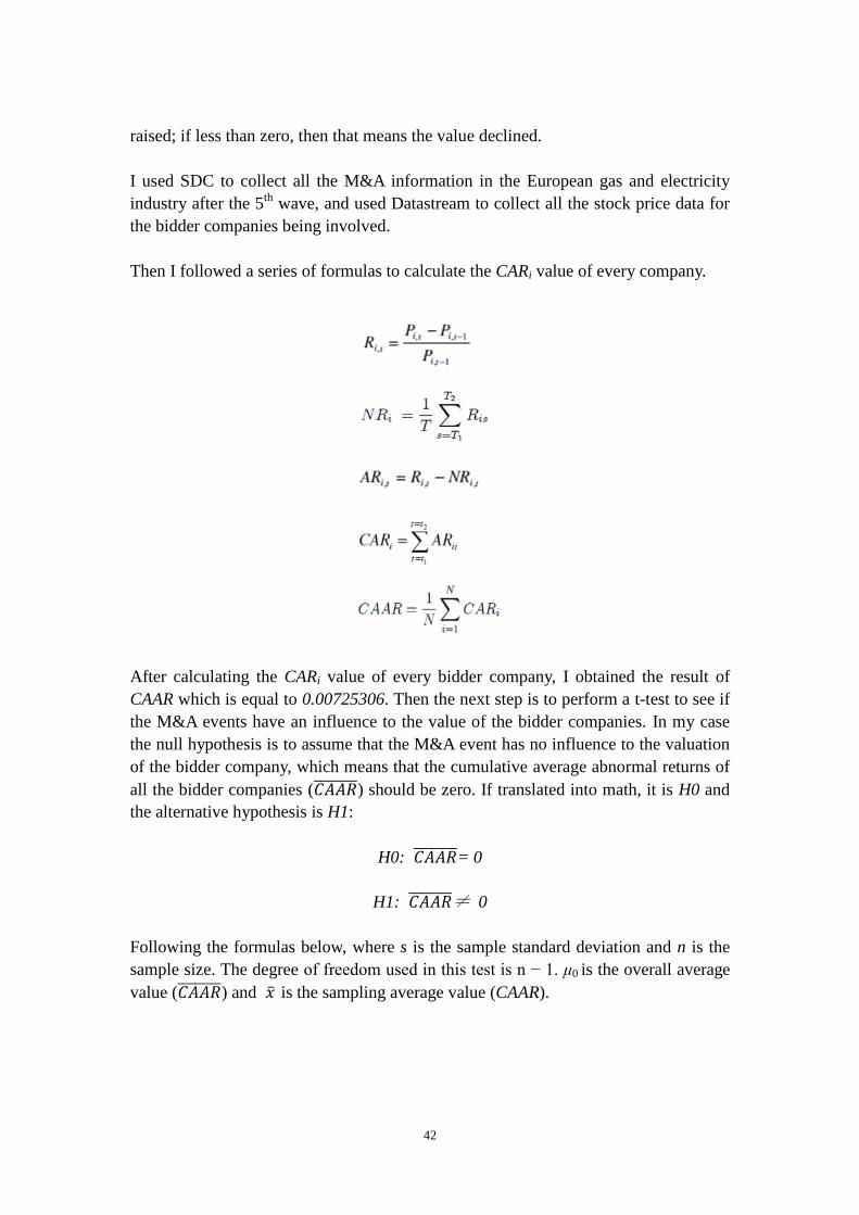
In the second step of my data collection, what I have obtained from the Datastream

database is the historical daily stock price of each bidder company. To calculate the

normal return of a stock, I need to first know the daily stock return. Thus to calculate

the daily return, I need to use the following formula:

where i is the stock index and t refers to time (day). R i,t is the stock return for day t

and stock i; Pi,t is stock price for day t and stock i. The result of the normal return

calculation is listed in Table 5 Normal returns of the bidder companies. For more detailed

intermediate data, you can also refer to attachment 2-normal return.

Table 5 Normal returns of the bidder companies

4.2.3 Calculate and analyze the abnormal returns

Abnormal return is defined as the difference between the actual return and the normal

return, which is illustrated in formula as:

27

Where ARi,t is the abnormal return of stock i on day t; Ri,t is the actual return of stock i

on day t; NRi,t is the normal return of stock i on day t. The calculation result of the

abnormal returns is stored in attachment 3 in details.

To analyze the result of the abnormal returns calculation, I construct a matrix of these

abnormal returns:

ARi,t is the abnormal return of stock i on day t; t = 0 is defined as the event date.

Therefore every column of the matrix represents the abnormal returns of one company

stock, and every row represents all the abnormal returns of every company on the

same day t. If there is more than one event happened on one company, then I treat it as

separate stocks (different columns). The result of the matrix is stored in attachment 3

in details.

Since I am interested in the performance of an interval, I aggregated the abnormal

returns from period [t1, t2] as the cumulative abnormal returns (CARi) of stock i.

The result of the CARi values is displayed in Table 6 Cumulative abnormal returns of the

bidder companies. Then I calculate the cumulative average abnormal returns of all the

stocks, and it is defined as:

After calculation, the result of CAAR is equal to 0.00725306, and the next step is to

perform a statistical test. In this section, the purpose is to test if the M&A events have

an influence to the value of the bidder companies. Here I adopt the t-test method as

my tool to solve the issue. T-test requires setting up a null hypothesis first; in my case,

that is the M&A event has no influence to the valuation of the bidder company, which

means that the cumulative average abnormal returns of all the bidder companies

should be zero. If translated into math, it is H0 and the alternative hypothesis is H1:

28

H0: = 0

H1: ≠ 0

Table 6 Cumulative abnormal returns of the bidder companies

Note that I have calculated the value of a CAAR, but that is the cumulative average

abnormal returns of the sampling bidder companies; while is the cumulative

average abnormal returns of all the bidder companies, which means covers

the complete set of the bidder companies but CAAR not.

The t-test statistical formula is:

where s is the sample standard deviation and n is the sample size. The degree of

freedom used in this test is n − 1. μ0 is the overall average value ( ) and is the

sampling average value (CAAR). s is calculated as:

29

After calculation, the value of s is 0.162044302, and as a result t is equal to

0.319648464. Looking into the t-test value table (double side, statistical significance

0.05), using the degree of the freedom as 50 (N - 1), t0.05 (50) = 2.0090. Since |t|<

t0.05 (50), referencing Table 7 | t | value, P value and the statistical conclusion, I can draw

the conclusion that:

Conclusion 1: H0 cannot be rejected, so I cannot consider that the M&A event

has no influence to the value of the bidder companies. In another word, it may

influence the value of the bidder companies.

α (statistical significance ) |t| P Conclusion

0.05 ＜t0.05（N-1） >0.05 H0 cannot be rejected; no statistical significance

0.05 >= t0.05（N-1） <= 0.05

Reject H0 and accept H1; there is statistical

significance

Table 7 | t | value, P value and the statistical conclusion

4.3 Research methodologies – Regression Analysis

4.3.1 Observed factors

The second research question is to find out what factors in M&A affect the bidder

companies‟ valuation change, and how much they affect the valuation change. In my

thesis, I will choose three factors to research:

if the location of the target where M&A took place is cross-border

if acquisition technique is privatization

if the payment is by cash

The first factor is about the target location. The issue of the cross-border takeover

becomes more and more concerned since the 5th

M&A wave occurred. Some

researchers believe that the fifth wave is actually the first international wave because

of the fast growing cross-border takeover in that period [14]. So I am interested to

know whether the M&A target location (cross-border or not) influences the valuation

change of a company after the 5th

wave.

The second observed element is the acquisition technique of the M&A, especially the

privatization. As the privatization is one of the characteristics of the new M&A in

electricity and gas industry after the 5th

wave, and it becomes a more and more

general way of the acquisition techniques after the 5th

wave mainly in distribution and

transmission networks. Therefore I want to find out what the effect of this feature is to

30

the valuation change of the bidder companies.

And last but not the least factor is the payment method of the deals. Normally the

bidder companies prefer to pay by cash compared to pay by equity, because equity

payment pattern declines more than payment by cash [3]. Based on this point I want

to research whether the cash payment has a positive effect to the valuation change to

the bidder companies.

4.3.2 To formulate the relationship between CAR and the factors

As I have explained in the earlier sections, the valuation change of a company can be

represented by the abnormal return, and since I observer a company during an event

period, I use the cumulative abnormal return (CAR) over the event period as the

quantitative representative of the valuation change of a company. So to study the

relationship between the valuation change of a company and the three factors is to

find out what the relationship is between CAR and the three factors.

The method I will use for this study is regression analysis. Regression analysis is a

method, which is based on obtaining massive data, and use statistical method to

formulate the relationship between dependent variables and independent variables as a

model function. In my research, the dependent variable is the cumulative abnormal

return (CAR), and the independent variables are the three factors that I want to

observe. Besides, normal return (NR) may have an influence to CAR, so although I am

not interested in if it really affects CAR or how it affects CAR, to make the

formulation more precise, I will also include NR as an independent variable.

Depends on the relationship between the dependent variable and the independent

variables, the model function can be linear or non-linear. A linear regression analysis

is a lot easier than a non-linear regression analysis, and usually if the model function

is non-linear, people will try to convert it to a linear function. To simplify the research,

I assume that this model function should be linear. For more detailed introduction

about regression analysis, you can refer to [31].

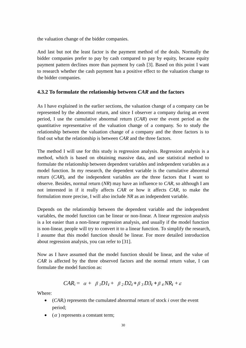
Now as I have assumed that the model function should be linear, and the value of

CAR is affected by the three observed factors and the normal return value, I can

formulate the model function as:

CARi = + 1D1i + 2 D2i + 3 D3i + 4 NRi +

Where:

(CARi) represents the cumulated abnormal return of stock i over the event

period;

( ) represents a constant term;

31

(D1i) represents the location of the target, where (1) is cross border and (0) is

domestic;

(β1) represents the coefficient of D1i ;

(D2i) represents the acquisition technique, where (1) is privatization and (0) is

for others;


(D3i) represents the means of payment, where (1) is by cash and (0) is by other

methods;


(NRi) represents the normal return.

(β4) represents the coefficient of NRi;

(ε) represents a noise term reflecting other factors that influence CARi .

β1, β2, and β3 represent the strength that the corresponding independent variable

affects the dependent variable. My purpose is to use regression analysis to produce an

estimate of β1, β2, and β3, and the tool I am going to use to help me do the regression

analysis is SPSS.

4.3.3 Regression Analysis by SPSS

SPSS is a computer program used for statistical analysis. Between 2009 and 2010 the

premier vendor for SPSS was called PASW (Predictive Analytics Soft Ware) Statistics,

while copyright issues for the name were settled. The company announced July 28,

2009 that it was being acquired by IBM and as of January 2010, it became "SPSS: An

IBM Company" [30].

To start the regression analysis using SPSS, I need to first prepare the input data file,

which contains the data of CAR, Crossboarder (D1), Privatization (D2), Cash (D3)

and NormalReturn (NR). The input data is stored in attachment 4, which is an Excel

sheet, but later converted to the format that SPSS recognizes. After the input file is

ready, the next step is to start the real regression analysis.

(1) Analyze Crossboarder (D1)

First I analyze only the relationship between CAR and Crossboarder, and the syntax I

use is:

regression

/dependent CAR

/method=enter Crossboarder

32

I use the regression command for running this regression. The /dependent

subcommand indicates the dependent variable, and the variables following

/method=enter are the predictors (independent variables) in the model. This is

followed by the output of these SPSS commands.

Variables Entered/Removedb

Model

Variables

Entered

Variables

Removed Method

1 Crossboardera . Enter

a. All requested variables entered.

b. Dependent Variable: CAR

Model Summary

Model R R Square

Adjusted R

Square

Std. Error of the

Estimate

1 .011a .000 -.020 .1636801468747

a. Predictors: (Constant), Crossboarder

ANOVAb

Model Sum of Squares Df Mean Square F Sig.

1 Regression .000 1 .000 .006 .941a

Residual 1.313 49 .027

Total 1.313 50

a. Predictors: (Constant), Crossboarder


Coefficientsa

Model

Unstandardized Coefficients

Standardized

Coefficients

t Sig. B Std. Error Beta

1 (Constant) .009 .030 .288 .775

Crossboarder -.003 .046 -.011 -.075 .941

a. Dependent Variable: CAR

The output is saved in attachment 4. The coefficient of Crossboarder is b=-0.003

which indicates that Crossboarder has a very minor influence to the value of CAR.

The significance of Crossboarder is sig=0.941, and because it is greater than 0.05,

that means the coefficient is not significantly different from zero. As a result, it seems

that Crossboarder is not related to the value of CAR, however, this model is only

using a single factor Crossboarder as the independent variable, so maybe if I include

33

this factor together with the others in the model, the analysis result may be different. I

will run the regression analysis with all the observed factors in part (4), and for more

detailed explanation about the SPPSS output, you can refer to part (5) in this section.

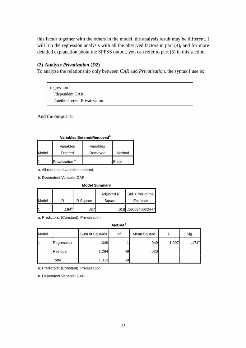
(2) Analyze Privatization (D2)

To analyze the relationship only between CAR and Privatization, the syntax I use is:

And the output is:


Model

Variables

Entered

Variables

Removed Method

1 Privatization a . Enter



Model Summary

Model R R Square

Adjusted R

Square

Std. Error of the

Estimate

1 .194a .037 .018 .1605940023447

a. Predictors: (Constant), Privatization

ANOVAb

Model Sum of Squares df Mean Square F Sig.

1 Regression .049 1 .049 1.907 .174a

Residual 1.264 49 .026

Total 1.313 50

a. Predictors: (Constant), Privatization


regression

/dependent CAR

/method=enter Privatization

34

Coefficientsa

Model


Standardized

Coefficients


1 (Constant) .021 .024 .843 .403

Privatization -.085 .062 -.194 -1.381 .174


The coefficient of Privatization is b=-0.085 which indicates that Privatization has a

very minor influence to the value of CAR. The significance of Privatization is

sig=0.174, and because it is greater than 0.05, that means the coefficient is not

significantly different from zero. As a result, it seems that Privatization is not related

to the value of CAR, however, this model is only using a single factor Privatization as

the independent variable, so maybe if I include this factor together with the others in

the model, the analysis result may be different. I will run the regression analysis with

all the observed factors in part (4), and for more detailed explanation about the SPSS

output, you can refer to part (5) in this section.

(3) Analyze Cash (D3)

To analyze the relationship only between CAR and Cash, the syntax I use is:

And the output is:


Model

Variables

Entered

Variables

Removed Method

1 Casha . Enter



regression

/dependent CAR

/method=enter Cash

35

Model Summary

Model R R Square

Adjusted R

Square

Std. Error of the

Estimate

1 .226a .051 .032 .1594427403850

a. Predictors: (Constant), Cash

ANOVAb


1 Regression .067 1 .067 2.645 .110a

Residual 1.246 49 .025

Total 1.313 50

a. Predictors: (Constant), Cash


Coefficientsa

Model


Standardized

Coefficients


1 (Constant) -.015 .026 -.575 .568

Cash .081 .050 .226 1.626 .110


The coefficient of Cash is b=0.081 which indicates that Cash has a very minor

influence to the value of CAR. The significance of Cash is sig=0.110, and because it

is greater than 0.05, that means the coefficient is not significantly different from zero.

As a result, it seems that Cash is not related to the value of CAR, however, this model

is only using a single factor Cash as the independent variable, so maybe if I include

this factor together with the others in the model, the analysis result may be different. I

will run the regression analysis with all the observed factors in part (4), and for more

detailed explanation about the SPPSS output, you can refer to part (5) in this section.

(4) Analyze Crossboarder, Privatization, Cash and NormalReturn

I have analyzed Crossboarder, Privatization, Cash separately, and it seems that they

are all unrelated to the value of CAR, however to make my analysis more precise, I try

to analyze them all together with normal return again. The syntax is:

36

And the output is:


Model

Variables

Entered

Variables

Removed Method

1 NormalReturn,

Privatization ,

Crossboarder,

Casha

. Enter



Model Summary

Model R R Square

Adjusted R

Square

Std. Error of the

Estimate

1 .288a .083 .003 .1617637695523

a. Predictors: (Constant), NormalReturn, Privatization , Crossboarder,

Cash

ANOVAb


1 Regression .109 4 .027 1.043 .395a

Residual 1.204 46 .026

Total 1.313 50

a. Predictors: (Constant), NormalReturn, Privatization , Crossboarder, Cash


regression

/dependent CAR

/method=enter Crossboarder Privatization Cash NormalReturn

37

Coefficientsa

Model


Standardized

Coefficients


1 (Constant) .010 .041 .252 .802

Crossboarder -.024 .048 -.073 -.499 .620

Privatization -.077 .064 -.174 -1.202 .236

Cash .076 .053 .212 1.435 .158

NormalReturn -2.083 27.121 -.011 -.077 .939


The output is saved in attachment 4. The analysis result seems to be unchanged

compared to the previous analysis.

None of the factors, Crossboarder (b=-0.024, sig=0.620), Privatization

(b=-0.077, sig=0.236), or Cash (b=0.076, sig=0.158) is related to the value of

CAR;

In table “ANOVA”, the significance value is 0.395, which indicates the

independent variables do not show a significant relationship to the dependent

variable;

In table “Model Summary”, the value of R Square (0.083) and the value of

Adjusted R Square (0.003) are so different, which is very possibly caused by

that the input data for the regression analysis is not sufficient (I have 51 input

data for the regression analysis). To verify that I need to obtain more data and

run the analysis again in the future.

In the following section, I will illustrate the output parameters by SPSS and then draw

a final conclusion about the second research question.

(5) Explanation of the SPSS output

To explain the output parameters by SPSS, I will take the analysis (4) as the example,

which is more meaningful, because that regression analysis includes all the

independent variables.

Table “Variables Entered/Removed” is a summary of the analysis, showing that CAR

is the dependent variable and Crossboarder, Privatization, Cash and NormalReturn,

are the independent variables.

Table “Model Summary”:

R is the square root of R Square (the next column).

R Square is the proportion of variance in the dependent variable which can be

predicted from the independent variables. In analysis (4), this value indicates

38

that 8.3% of the variance in CAR can be predicted from the independent

variables.

Adjusted R square. In simplicity, the closer this value is to R Square, the

better the regression analysis is. When the number of the input data is small,

while the number of observed independent variables is large, there will be a

great difference between R Square and Adjusted R square (as in my analysis,

where R Square is 0.083, while Adjusted R Square is 0.003). By contrast,

when the number of the input data is large, and the number of observed

independent variables is small, the value of R Square and Adjusted R Square

will be very close.

Std. Error of the Estimate is the standard deviation of the error term.

Table “ANOVA”: the Total variance is partitioned into the variance which can be

explained by the independent variables (Regression) and the variance which is not

explained by the independent variables (Residual).

Sum of Squares are the Sum of Squares associated with the three sources of

variance, Total, Regression & Residual. The Sums of Squares for the

Regression and Residual add up to the Total Variance, reflecting the fact that

the Total Variance is partitioned into Regression and Residual variance.

df: These are the degrees of freedom associated with the sources of variance.

The total variance has N-1 degrees of freedom. Again the sum of the

Regression df and Residual df is equal to the Total df.

Mean Square: the Mean Squares is calculated as, the Sum of Squares divided

by their respective df.

F: The F Value is the Mean Square Regression divided by the Mean Square.

Sig.: this value is the p value associated with the F value. You can use this

value to answer the question "Do the independent variables reliably predict the

dependent variable?" The p value is compared to the alpha level (typically

0.05) and, if smaller, it can be concluded "Yes, the independent variables

reliably predict the dependent variable". If the p value were greater than 0.05,

you would say that the independent variable does not show a significant

relationship with the dependent variable, or that the independent variable does

not reliably predict the dependent variable. The p value in my regression

analysis is 0.395, which is far greater than 0.05, and as a result, the observed

independent variables do not show a significant relationship to the dependent

variable. In another word, the observed factors do not show a significant

influence to CAR.

Table “Coefficients”: this table quantifies the estimate of the coefficients and their

corresponding statistical significance.

B: this is the estimated value of the coefficient. Using these values, the

regression analysis model function can be formulated as:

39

CARi = 0.010 – 0.024 * D1i – 0.077 * D2i + 0.076 * D3i –2.083 * NRi + ε

Std.Error: These are the standard errors associated with the coefficients.

Standardized Coefficients: These are the standardized regression coefficients.

Since all the independent variables are standardized, you can compare the

strength that the independent variables affecting the dependent variable. In my

regression analysis result, it shows that the payment method has the greatest

influence to CAR.

t & sig: These columns provide the t value and 2 tailed p value used in testing

the null hypothesis that the coefficient/parameter is 0. The p value is compared

to your alpha level (typically 0.05), and if smaller, you can reject the null

hypothesis and say that that the coefficient is significantly different from 0; if

p is greater than 0.05, then you cannot reject the null hypothesis, which means

that the factor may be unrelated to the dependent variable. As my regression

analysis result shows, the p values of all the three observed factors are greater

than 0.05, which means they may have no influence to the value of CAR.

(6) Conclusion

The purpose of my regression analysis is to estimate how the following factors affect

the valuation change of a company (CAR).

(D1) if the location of the target where M&A took place is cross border

(D2) if acquisition technique is privatization

(D3) if the payment is by cash

I did four times regression analysis, and every factor has been estimated twice (once

separately and once together will all the other factors). Both two times the coefficients

of all the three factors are very little numbers, and all the p values are greater than

0.05 (see Table 8 Coefficient estimation and the statistical significance), which indicates that

the coefficients are not significantly different from zero (in another word, the three

factors are not related to the valuation change of the company)

Dependent

variable

Separate analysis Combined analysis

B Sig. B Sig.

Crossboarder -0.003 0.941 -0.024 0.62

Privatization -0.085 0.174 -0.077 0.236

Cash 0.081 0.11 0.076 0.158

Table 8 Coefficient estimation and the statistical significance

In table “Model Summary”, the value of R Square (0.083) and the value of Adjusted

R Square (0.003) are so different, which means that the input data for the regression

analysis is not sufficient.

40

Conclusion 2: all the three factors (if the location of the target where M&A took

place is cross border or domestic, if acquisition technique is privatization, and if

the payment is by cash) are not related to the valuation change of the bidder

company. However, to confirm my conclusion, I need to do the regression

analysis further based on more data.

41

Chapter 5 Summary and Conclusions

5.1 Literature review, opportunities and barriers

I did my research on the mergers and acquisitions of the European electricity and gas


wave. In Chapter 2 Literature review, I introduced the history of

M&A, which has gone through six waves, and also the classification of the M&A (the

difference among Merger and Consolidation, Acquisition of Stock, and Acquisition of

Assets). Moreover I specified the characteristics of the M&A in gas and electricity

sector, which are mainly restructuring, competition, regulation and privatization.

In Chapter 3, I illustrated the opportunities and the barriers of the M&A after the 5th

wave, which aims to clarify the possibility and the difficulty of the bidder and target

companies experienced or will experience. After the fifth wave the requirements on

the private distribution and transmission of the electricity and gas industry become

more and more, so it is a good opportunity to operate the restructuring. And of course

there will be somehow the difficulties alongside with the process like higher entry

barrier and too relaxed standards of the M&A in electricity and gas industry in

Europe.

Then I raised up my two research questions. And I used event study and regression

analysis to study them respectively.

(1) Is the stock value of the observed bidder companies in European electricity and

gas industry significantly affected by the mergers and acquisitions?



5.2 Event Study

In order to research whether the M&A has an effect on the valuation of the bidder

companies after the 5th

wave in the European gas and electricity industry, I used SDC

and Datastream as the tool / database to collect data and perform an event study to

find out the result.

As Fama, Fisher, Jensen and Roll [5] proposed, I compared the stock return around

the M&A time (event window) and the normal stock return prior to the M&A event

(estimation window [T1, T2]) to represent if the value of the company has been

changed. The difference between the actual stock return (Ri,t) and the normal stock

return (NRi) is called abnormal return (ARi,t), and the sum of the abnormal return of a

stock during the event window is called cumulative abnormal return. If the cumulative

abnormal return (CARi) is greater than zero, that means the value of the company has

42

raised; if less than zero, then that means the value declined.

I used SDC to collect all the M&A information in the European gas and electricity


wave, and used Datastream to collect all the stock price data for

the bidder companies being involved.

Then I followed a series of formulas to calculate the CARi value of every company.

After calculating the CARi value of every bidder company, I obtained the result of

CAAR which is equal to 0.00725306. Then the next step is to perform a t-test to see if

the M&A events have an influence to the value of the bidder companies. In my case

the null hypothesis is to assume that the M&A event has no influence to the valuation

of the bidder company, which means that the cumulative average abnormal returns of

all the bidder companies ( ) should be zero. If translated into math, it is H0 and

the alternative hypothesis is H1:

H0: = 0

H1: ≠ 0

Following the formulas below, where s is the sample standard deviation and n is the

sample size. The degree of freedom used in this test is n − 1. μ0 is the overall average

value ( ) and is the sampling average value (CAAR).

43

After calculation, the value of s is 0.162044302, and t is equal to 0.319648464.

Looking into the t-test value table (double side, statistical significance 0.05). I can

draw the conclusion that, H0 cannot be rejected, which means, M&A event may


5.3 Regression Analysis

If the M&A event may influence the valuation of the bidder companies, what factors

in the M&A event would actually influence the value of CAR, and that is my second

research question. In my thesis, I researched three factors below to see if they have

affected CAR.

if the location of the target where M&A took place is cross-border

if acquisition technique is privatization

if the payment is by cash

First of all, I analyze all the three factors separately, and the results show that they are

not related to the value of CAR, because the coefficients are all very little numbers,

and the significance values show that the coefficients are not significantly different

from zero (Sig. > 0.05). For convenience, I copy the result data below to see the

coefficient of every factor and their corresponding significance.

(1) Cross boarder:

Coefficientsa

Model


Standardized

Coefficients


1 (Constant) .009 .030 .288 .775

Crossboarder -.003 .046 -.011 -.075 .941


44

(2) Privatization:

Coefficientsa

Model


Standardized

Coefficients


1 (Constant) .021 .024 .843 .403

Privatization -.085 .062 -.194 -1.381 .174


(3) Payment by cash:

Coefficientsa

Model


Standardized

Coefficients


1 (Constant) -.015 .026 -.575 .568

Cash .081 .050 .226 1.626 .110


And next I analyzed all the three factors together, the regression analysis model

function is

CARi = + 1D1i + 2 D2i + 3 D3i + 4 NRi +

Where D1i represents the location of the target, where (1) is cross border and (0) is

domestic; D2i represents the acquisition technique, where (1) is privatization and (0)

is for others; D3i represents the means of payment, where (1) is by cash and (0) is by

other methods; NRi represents the normal return. β1, β2, β3 and β4 represent the

strength that the corresponding independent variable affects the dependent variable.

The result shows that the three factors are still not related to the value of CAR.

However, the value of R Square and the value of Adjusted R Square are too different,

which means that the regression analysis result is not accurate, and I need to use more

data for further analysis. For convenience, the result table is listed below.

45

Model Summary

Model R R Square

Adjusted R

Square

Std. Error of the

Estimate

1 .288a .083 .003 .1617637695523

a. Predictors: (Constant), NormalReturn, Privatization , Crossboarder,

Cash

Coefficientsa

Model


Standardized

Coefficients


1 (Constant) .010 .041 .252 .802

Crossboarder -.024 .048 -.073 -.499 .620

Privatization -.077 .064 -.174 -1.202 .236

Cash .076 .053 .212 1.435 .158

NormalReturn -2.083 27.121 -.011 -.077 .939


5.4 Conclusions

As discussed in chapter 4, the two conclusions I draw are:

Conclusion 1: H0 cannot be rejected, so I cannot consider that the M&A event

has no influence to the value of the bidder companies. In another word, it may


Conclusion 2: all the three factors (if the location of the target where M&A took

place is cross border, if acquisition technique is privatization, and if the payment

is by cash) are not related to the valuation change of the bidder company.

However, this conclusion may be not accurate due to limited number of input

data. To confirm my conclusion, I need to do the regression analysis further

based on more data.

46

REFERENCE

[1] Frank de Jong, 2007. “Event Studies Methodology”, Tilburg University.

[2]http://www.tilburguniversity.edu/nl/over-tilburg-university/bibliotheek/ibutton/SDCmanual.doc

[3] Renneboog, L., 2006. “Advances in Corporate Finance and Asset Pricing”, Elsevier.

[4] http://online.thomsonreuters.com/Datastream/

[5] Fama, Eugene, Lawrence Fisher, Michael Jensen and Richard Roll, 1969. “Market efficiency,

long-term returns, and behavioral finance”, Journal of Financial Economics 49, 283-306.

[6] Bowman, Robert, 1983. “Understanding and conducting event studies”, Journal of Business

Finance and Accounting 10, 561-584.

[7] Brown S. and Warner J., 1980. “Measuring security price performance”, Journal of Financial

Economics, Vol. 8, pp. 205-258.

[8] Loi Lei Lai, 2001. “Power system restructuring and deregulation: Trading, Performance and

Information Technology”.

[9] Pavel Stehlik, January 2006. “The effects of politics on energy M&A: Central European and

CIS regions”.

[10] Sudarsanam S., 2003, “Creating Value from Mergers and Acquisitions: The Challenges”.

[11] Devra L Golbe & Lawrence J. White, 1993, “Catch a Wave: The Time Series Behavior of

Mergers”, The Review of Economic and Statistics, Vol. 75, No. 3, Aug 1993.

[12] Kees Cools & Mindel van de Laar, 2006, “The Performance of Acquisitive Companies”,

Advances in Corporate Finance and Asset Pricing.

[13] Martin Lipton, September 2006, “Merger Waves in 19th, 20th and 21st Centuries”, York

University.

[14] Bernard S. Black, 2000, “The First International Merger Wave (and the Fifth and Last US

wave)”, Stanford Law School: May 2000, Working Paper no. 199.

[15] Skadden: “Trends in European Merger and Acquisitions”, European Merger and Acquisition,

Leaders Magazine Inc., Volume 29, no. 4

[16] Tooraj Jamasb and Michael Pollitt, March 2005, “Electricity Market Reform in the European

http://www.tilburguniversity.edu/nl/over-tilburg-university/bibliotheek/ibutton/SDCmanual.doc

http://online.thomsonreuters.com/datastream/

47

Union, Review of Progress toward Liberalization & Integration”.

[17] Mariusz Przybylik., June 2005, “Implications and Recommendations for Restructuring of

Electric Power Distribution.”

[18] Marc-Kévin Codognet, Jean-Michel Glachant, Céline Hiroux, Matthieu Mollard, François

Lévêque, Marie-Anne Plagnet., July 2003,”Mergers and Acquisitions in the European Electricity

Sector,Cases and Patterns”, Paris France

[19] Gilardi, Fabrizio, 2002, “Delegation to Independent Regulatory Agencies: Insights from

Rational”.

[20] Eric van Damme, 2005, "Liberalizing the Dutch Electricity Market: 1998-2004," The Energy

Journal, International Association for Energy Economics, vol. 26(Special I), pages 155-180

[21] Jamasb, T. 2002, “Reform and Regulation of the Electricity Sectors in Developing Countries.

DAE working Paper 0226 (CMI EP 08), Department of Applied Economics, University of

Cambridge.

[22] Newbery, D. 2002a, “Issues and Options for Restructuring Electricity Supply Industries.”

Cambridge Working Papers in Economics 0210 / CMI Working Paper CMI EP 01, Department of

Applied Economics, University of Cambridge.

[23] Arentsen, M. J., J. W. Fabius and R. W. Kunneke , 2001, “Dutch Business Strategies under

Regime Transition.” In Midttun, A. (ed.), European Energy Business Strategies, Elsevier:

London.

[24] Pollitt, M. 1999, “Issues in Electricity Market Integration and Liberalization, in An

European Market for Electricity?” In Bergman, L. et al., Monitoring European Deregulation 2,

Centre for Economic Policy Research, October, London.

[25] Pollitt, M.G. 2004, “Electricity Reform in Chile: Lessons for Developing Countries.”

Journal of Network Industries 5(3-4): 221-262.

[26] Joskow, P. L. 2003, “Electricity Sector Restructuring and Competition: Lessons Learned.”

Working Paper 2003-014, Center for Energy and Environmental Policy Research, Massachusetts

Institute of Technology.

[27] Vickers, J., and G. Yarrow, 1988, Privatization: An Economic Analysis. Cambridge:MIT

Press. van Damme, E, 2005,“Liberalizing the Dutch Electricity Market: 1998-2004” Energy

Journal.

[28] Newbery, D. and M. Pollitt , 1997,“Restructuring and Privatization of the CEGB - Was It

http://ideas.repec.org/a/aen/journl/2005se-a07.html

http://ideas.repec.org/s/aen/journl.html

http://ideas.repec.org/s/aen/journl.html

48

Worth It?”Journal of Industrial Economics 45(3), 269-304.

[29] Richard E. Caves, “Effects of Mergers and Acquisitions on the Economy: An Industrial

Organization Perspective”, Harvard University.

[30] http://en.wikipedia.org/wiki/SPSS

[31] Alan O.Sykes, “An Introduction to Regression Analysis”, University of Chicago

event study analysis: comparison of mergers and

Documents