evaporation change and global warming: the role of net

Evaporation change and global warming: The roleof net radiation and relative humidity

David J. Lorenz,1 Eric T. DeWeaver,1 and Daniel J. Vimont1

Received 26 January 2010; revised 24 June 2010; accepted 12 July 2010; published 29 October 2010.

[1] The change in evaporation over the oceans in climate models is analyzed from theperspective of air‐sea turbulent fluxes of water and energy. The results challenge the viewthat the change in evaporation is predominantly constrained by the change in the netradiation at the surface. For fixed net radiation change, it is found that (1) robust increasesin near‐surface relative humidity and (2) robust decreases in turbulent exchange coefficientlead to a substantial reduction in evaporation below the rate of increase implied by the netradiation alone. This reduction of evaporation is associated with corresponding changes inthe sensible heat flux. In addition, a net imbalance in the surface energy budget undertransient greenhouse gas forcing provides a further reduction in the evaporation change inclimate models. Further results also suggest that it might be more physical to view theevaporation change as a function of relative humidity change rather than net radiation. Inthis view, the relative humidity controls the net surface shortwave radiation throughchanges in low‐level cloudiness and the temperature controls the net surface radiationthrough the changes in longwave radiation. In addition, the results demonstrate thedominant role of both the air‐sea temperature difference and relative humidity over, forexample, wind speed in reducing the evaporation change in climate models below theClausius‐Clapeyron rate.

Citation: Lorenz, D. J., E. T. DeWeaver, and D. J. Vimont (2010), Evaporation change and global warming: The role of netradiation and relative humidity, J. Geophys. Res., 115, D20118, doi:10.1029/2010JD013949.

1. Introduction

[2] In response to global warming, climate models predictthat global‐mean precipitation will increase with surface airtemperature at a rate of about 1% to 3% per degree Kelvin[Boer, 1993; Allen and Ingram, 2002; Allan and Soden,2007]. This change in precipitation is substantially smallerthan the change in atmospheric water vapor, which increasesat the Clausius‐Clapeyron (CC) rate of 6% to 7% per Kelvin[Boer, 1993; Allen and Ingram, 2002; Held and Soden,2006]. Recently, Wentz et al. [2007] have reported trendsin “observed” precipitation that are about three times largerthan the climate models and more in line with the CC rate.The difference between modeled and observed estimates ofprecipitation change indicate that (1) models are lacking theessential physical processes that generate the correct changesin precipitation [Wentz et al., 2007; Allan and Soden, 2007],(2) observed estimates of global precipitation are inadequatefor determining trends in precipitation due to globalwarming [Previdi and Liepert, 2008; Lambert et al., 2008], or(3) precipitation variations in the observed record are not yetdominated by the precipitation response to global warming[Allen and Ingram, 2002; Previdi and Liepert, 2008].

[3] Why do models predict an increase in precipitationthat is substantially below the CC rate? The answer appearsbe to the dominant role that the hydrologic cycle plays in theglobal energy budget [Boer, 1993; Allen and Ingram, 2002;Pierrehumbert, 2002; Lambert and Allen, 2009]. In thetroposphere, the dominant balance in the time‐mean atmo-spheric energy budget is between radiative cooling andlatent heating from precipitation, and as such changes inprecipitation are generally assumed to be constrained by theability of the atmosphere to radiate away heat generated bycondensation [Allen and Ingram, 2002]. This view generallyassumes a negligible change in the sensible heat flux fromthe surface to the atmosphere and therefore assumes thatlarge trends in “observed” precipitation must be accompa-nied by large changes in the net radiative cooling of theatmosphere.[4] Our analysis differs from the analysis in Allen and

Ingram [2002] in that we address changes in the hydro-logical cycle through the surface energy budget rather thanthe atmospheric energy budget. We believe that an analysisin terms of the surface energy budget makes quantitativeassessment of the relative roles of latent and sensible heatmuch easier. Indeed, we find that changes in the sensibleheat flux are not negligible and in some climate models caneven be larger than the net radiation change at the surface.Formally, our consideration of the surface energy budget isthe same as the atmospheric energy budget of Allen andIngram [2002] if equilibrium is assumed and sensible heat

1Center for Climatic Research, Madison, Wisconsin, USA.

Copyright 2010 by the American Geophysical Union.0148‐0227/10/2010JD013949

JOURNAL OF GEOPHYSICAL RESEARCH, VOL. 115, D20118, doi:10.1029/2010JD013949, 2010

D20118 1 of 13

http://dx.doi.org/10.1029/2010JD013949

flux is ignored; the equivalence of the two methods is adirect result of zero change in the top of the atmosphereradiative heat flux.[5] In this paper, we analyze the changes in evaporation

and sensible heat in climate models from the perspective ofair‐sea turbulent fluxes of water and energy over the oceans:

E ¼ k qs Tsð Þ � rqs Tað Þð Þ; ð1Þ

S ¼ kcp Ts � Tað Þ; ð2Þ

where E is the evaporation, S is the sensible heat flux, qs(T )is the saturation specific humidity as a function of temper-ature, r is the relative humidity, k is the turbulent exchangecoefficient that depends on wind speed and static stability,cp is the specific heat of air at constant pressure, and thesubscripts s and a refer to the sea surface temperature (SST)and near surface air temperature, respectively. Our studybegins with an analysis similar to Richter and Xie [2008],who showed that changes in the air‐sea temperature differ-ence, relative humidity and k are important for reducing theevaporation change below the CC rate. The remainder ofthe paper analyzes the evaporation change by consideringthe constraints imposed by the surface energy budget. Byrecasting the energy budget in terms of the air‐sea temper-ature difference, we show that given the change in netradiation at the surface and certain assumptions about rela-tive humidity and k, one can calculate the equilibriumchange in evaporation. Using this framework for calculatingevaporation we provide answers to the following: Given thehypothesis that evaporation is primarily constrained by thenet radiation at the surface [Allen and Ingram, 2002], are thespecific mechanisms for reducing evaporation studied inRichter and Xie [2008] important for understanding the totalchange in evaporation or is the total change in evaporation

primarily determined by the net radiation alone? If in factevaporation changes at the CC rate [Wentz et al., 2007], thendoes this mean that the net radiation at the surface must alsoincrease at the CC rate?[6] In this study, we first ignore constraints imposed by

the energy budget and use the bulk formulae to quantify thevarious mechanisms that contribute to an evaporationchange that is different than the CC rate (section 3). We thencalculate which mechanisms are most important in climatemodels under global warming. In section 4, we take intoaccount the energy budget by calculating the changes inlatent and sensible heat fluxes as a function of the change innet radiation at the surface. We also quantify the relativeroles of relative humidity and turbulent exchange coefficientin generating the changes in fluxes in the climate models. Insection 5, we discuss the physical mechanisms that might beresponsible for the relationship between radiation, relativehumidity, and evaporation. In section 6, we discuss theimplications of these results for climate prediction, and wediscuss the possibility of detecting the changes in the air‐seatemperature difference and relative humidity in the observedrecord.

2. Data and Methods

[7] We use output from climate change scenario integra-tions prepared for the IPCC Fourth Assessment Report,archived by the Program for Climate Model Diagnostics andIntercomparison at the Lawrence Livermore National Labo-ratory. Future climate data used here comes from the A1Bscenario, a scenario in which carbon dioxide (CO2) con-centrations rise to 720 parts per million (ppm) by the year2100 and then remain fixed for the next 200 years (i.e. until2300). Simulations of present‐day climate from the samemodels were obtained from the Coupled Model Intercom-parison Project’s “20th Century Climate in Coupled Models”(20C3M) data archive. The variables available for eachmodel are listed in Table 1. Complete details on the forcingused in the A1B scenario is given in Appendix II of the 2001Intergovernmental Panel on Climate Change (IPCC) report[IPCC, 2001]. In the results presented here, climate change isdefined as the difference between the climatologies of years2080 to 2099 in the A1B scenario and years 1980 to 1999 inthe 20C3M simulations. We also look briefly at the changesobserved by 2180–2199 and by 2280–2299. The analysisis restricted to the oceans between the latitudes of 60°S and60°N because we wish to avoid the complications associatedwith soil moisture over land and sea ice poleward of 60°.Evaporation over oceans between 60°S and 60°N accountsfor 81% of the total surface evaporation (in the climatemodels). Moreover, the change in evaporation over oceansbetween 60°S and 60°N in a given climate model is a goodpredictor of the change in total evaporation in that climatemodel (correlation = 0.87) [see also Lu and Cai, 2009].[8] In the results presented here, we use the 1,000 mbar

relative humidity as the surface air relative humidity. Wehave repeated the analysis using the 2 meter specifichumidity and temperature and the results are very similar.We choose to use 1,000 mbar relative humidity instead of2 meter specific humidity because 22 models archived rela-tive humidity compared to 15 models that archived 2 meterspecific humidity. For the saturation vapor pressure, es, and

Table 1. The IPCC Models Used in This Studya

Model (CMIP3 I.D.) VariablesModel number

in Figures 1 and 2

bccr_bcm2_0 Ta, Ts, E, S, F, r 1cccma_cgcm3_1 Ta, Ts, E, S, F, r, us, vs 2cccma_cgcm3_1_t63 Ta, Ts, E, S, F, r, us, vs 3cnrm_cm3 Ta, Ts, E, S, F, r, us, vs 4csiro_mk3_0 Ta, Ts, E, S, r, us, vs 5csiro_mk3_5 Ta, Ts, E, S, F, r, us, vs 6gfdl_cm2_0 Ta, Ts, E, S, F, r, us, vs 7gfdl_cm2_1 Ta, Ts, E, S, F, r 8giss_model_e_h Ta, Ts, E, S, F, r 9giss_model_e_r Ta, Ts, E, S, r, us, vs 10iap_fgoals1_0_g Ta, Ts, E, S, F, r, us, vs 11ingv_echam4 Ta, Ts, E, S, r, us, vs 12Inmcm3_0 Ta, Ts, E, S, F, r, us, vs 13ipsl_cm4 Ta, Ts, E, S, F, r, us, vs 14miroc3_2_hires Ta, Ts, E, S, F, r, us, vs 15miroc3_2_medres Ta, Ts, E, S, F, r, us, vs 16mpi_echam5 Ta, Ts, E, S, F, r 17mri_cgcm2_3_2a Ta, Ts, E, S, F, r, us, vs 18ncar_ccsm3_0 Ta, Ts, E, S, F, r 19ncar_pcm1 Ta, Ts, E, S, r 20ukmo_hadcm3 Ta, Ts, E, S, F, r 21ukmo_hadgem1 Ta, Ts, E, S, F, r 22

aThe second column lists the variables available for that model (see textfor abbreviations of the variables).

LORENZ ET AL.: EVAPORATION CHANGE AND GLOBAL WARMING D20118D20118

2 of 13

the Clausius‐Clapeyron rate, 1es

desdT , we use the function given

byBolton [1980]. The saturation specific humidity’s in (1) arecalculated assuming the surface pressure is 1,000 mbar.Because the analysis is restricted to the ocean regions, this is agood approximation.[9] In this paper, we diagnose the temporal and spatial

mean of evaporation and sensible heat using the bulk for-mulas (1) and (2). We sometimes average over models, too.Because (1) and (2) are nonlinear, diagnosing E and S usingaverage k, q, and r can potentially be problematic. There-fore, for evaporation, we write

E ¼ kqs Tsð Þ � krqs Tað Þ; ð3Þ

where the overbar is an average over space, model, and timeand all variables depend on space, model and time. Wedefine k using

k ¼ E= qs Tsð Þ � rqs Tað Þð Þ: ð4Þ

The first term on the right‐hand side of (3), can be written

kqs Tsð Þ ¼ kqs Tsð Þ þ k0qs 0 Tsð Þ; ð5Þ

where primes denote deviations from the space, model, andtime average. For monthly data the second term in (5) is−8.1% times the first. For a 12 month climatology as thetime variable, the second term is −8.0% times the first, andthe magnitudes of the two terms are also very similar.Therefore, all variables analyzed are 12 month climatolo-gies. Richter and Xie [2008] investigated the effect of using(3) with daily data instead of a climatology and likewisefound that the deviations are small. Instead of (5), kqs Tsð Þcan also be written as

kqs Tsð Þ ¼ kkqs Tsð Þ

k

!¼ kqs Tsð Þ; ð6Þ

where the double overbar denotes an average of q weightedby k. The second term on the right of (3) can be written

krqs Tað Þ ¼ krqs Tað Þ þ k 0r0qs Tað Þþ rk 0qs0 Tað Þ þ kr0qs0 Tað Þ þ k 0r0qs 0 Tað Þ: ð7Þ

The magnitudes of terms 2 through 5 on the right‐hand siderelative to the first are 0.87%, −7.9%, −0.63% and −0.02%for climatological data, respectively. (As before, monthlydata are very similar.) Therefore we are justified in keepingthe first and third terms and disregarding the rest and thusthe second term on the right of (3) can also be written in theform

krqs Tað Þ ¼ krqs Tsð Þ; ð8Þ

where, once again, the double overbar denotes an averageweighted by k. For the sensible heat, the covariance termsare −0.5% times the magnitude of the mean term, andtherefore we neglect these terms, and temperature averagesare simple averages that are not weighted by k. Hence allterms in (1) and (2) and all terms in all equations derivedfrom them below are understood to be simple averagesexcept for q, which are averages weighted by the spatial,

model, and temporal variability in k. When we make theseapproximations, the mean latent heat flux given by the bulkformula is 109.6Wm−2 instead of the true value of 108.7Wm−2

(0.78% error). To more easily compare changes in q, weweight the future q the same as the present q (i.e., we weightthe future q by the 20th‐century k). The error introduced bythis is small: the approximate future latent heat is 114.9 W m−2

instead of 113.5 W m−2 (1.2% error).[10] One additional detail: the calculation of k using (4)

gives very large values when (qs(Ts) − rqs(Ta)) is small.Because we are using pressure level relative humidityinstead of surface relative humidity, the accuracy in r islikely at least 1%. Therefore, whenever ∣qs(Ts) − rqs(Ta)∣ <0.01 · qs(Ta), we set the humidity difference to be 0.01 ·qs(Ta) instead of (qs(Ts) − rqs(Ta)). This adjustment is per-formed 0.5% of the time.

3. Mechanisms of Evaporation Change

[11] In this section, we find the contributions of the air‐seatemperature difference, the relative humidity, and k to thefractional change in evaporation over the oceans using thebulk formula for evaporation (1), and quantify those con-tributions in the CMIP3 climate models. Changes in any oneof these three factors will cause E to deviate from the CCrate. Here, we consider these changes independent of con-straints imposed by the energy budget.[12] Precipitation and evaporation changes are typically

given by the fractional change per degree temperaturechange: 1

EdEdTa

¼ d lnEdTa

, where E is the evaporation and Ta isthe surface air temperature. By taking the derivative withrespect to air temperature of (1), we decompose the totalevaporation change into several components (Appendix A):

d lnE

dTa¼ �� 1� �ð Þ�qs Tsð Þ

qs Tsð Þ � rqs Tað Þ �dr

dTaqs Tað Þ

qs Tsð Þ � rqs Tað Þ þd ln k

dTa; ð9Þ

where a is the CC rate ( = 1qs

dqsdT ) and g is the ratio of the sea

surface temperature change to the near surface air temper-ature change ( = dTs

dTa). The second term on the right describes

the effect of changes in the air‐sea temperature difference onE, the third term on the right describes the effect of changesin the relative humidity on E, and the fourth term on theright describes the effect of the exchange coefficient(influenced by wind speed or vertical stability) on E. Notethat these three terms act to increase or reduce the evapo-ration rate from the CC rate, a: if k and r are constant and Tsand Ta increase by the same amount (i.e., g ≡ dTs

dTa= 1), then

the evaporation increases with temperature at the CC rate.[13] Because of the important role of the hydrologic cycle

on both the surface at atmospheric energy budget, however,the E change is in general not equal to the CC rate. Theconstraints imposed by the energy budget are most easilyseen by considering the evolution to equilibrium in responseto global warming. For example, consider the case where Tsand Ta increase by the same amount. If the remaining termsin the energy budget increase at a rate less than a, then theenergy budget is imbalanced and E will cool the surface(and will eventually heat the atmosphere when the watercondenses). This will act to increase Ta relative to Ts so thatg will be less than one (i.e., the air‐sea temperature differ-


3 of 13

ence decreases). The reduced air‐sea temperature differencewill decrease E through the second term on the right side of(9) and will eventually bring the energy budget into balance.In fact, E is quite sensitive to changes in g: substituting inthe average values for qs(Ts), qs(Ta), and r over the oceansbetween 60°S and 60°N, we find that the second term on theright in (9) is 4.3 · (1 − g) · a. Hence a g of 0.88 will give anE increase of 0.5a and a g of 0.77 will give zero E increase.For the climate models, Ts increases less than Ta with atypical value for g of 0.94.[14] The contribution of the second, third, and fourth

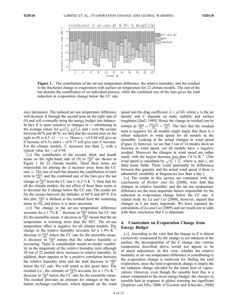
terms on the right‐hand side of (9) to d lnEdTa

are shown inFigure 1 for 22 climate models. These three terms areresponsible for altering the E increase away from the CCrate, a. The size of each bar denotes the contribution of eachterm to d lnE

dTa, and the combined size of the bars give the net

change in d lnEdTa

from the CC rate (= 6.2 % K−1). Note that forall the climate models, the net effect of these three terms isto decrease the E change below the CC rate. The results arefor the oceans between the latitudes of 60°S and 60°N. Forthis plot, d ln k

dTais defined as the residual from the remaining

terms in (9), and hence it is more uncertain.[15] The change in the air‐sea temperature difference

accounts for a 1.7% K−1 decrease in d lnEdTa

below the CC ratefor the ensemble‐mean. A decrease in d lnE

dTameans that the air

temperature is warming more than the SST. The air‐seatemperature effect is negative for all climate models. Thechange in the relative humidity accounts for a 1.4% K−1

decrease in d lnEdTa

below the CC rate for the ensemble‐mean.A decrease in d lnE

dTameans that the relative humidity is

increasing. There is considerable model‐to‐model variabil-ity in the magnitude of the relative humidity term although20 out of 22 models show increases in relative humidity. Inaddition, there appears to be a positive correlation betweenthe relative humidity term and the total decrease in d lnE

dTabelow the CC rate. We will return to this point later. Theresidual (i.e., the estimate of d ln k

dTa) accounts for a 1.1% K−1

decrease in d lnEdTa

below the CC rate for the ensemble‐mean.The residual provides an estimate for changes in the tur-bulent exchange coefficient, which depends on the wind

speed and the drag coefficient: k = rC∣~u∣, where r is the airdensity and C depends on static stability and surfaceroughness [Stull, 1989]. Hence the change in residual can be

written as d ln kdTa

¼ d lnð�CÞdTa

þ d ln~uj jdTa

. The fact that the residualterm is negative for all models might imply that there is arobust reduction in wind speed for all models in theensemble. Looking at the actual changes in wind speed(Figure 2), however, we see that 3 out of 14 models show anincrease in wind speed, yet all models have a negativeresidual. Moreover the changes in wind speed are rathersmall, with the largest decrease less than 1.0 % K−1. (Thewind speed is calculated by

ffiffiffiffiffiffiffiffiffiffiffiffiffiffiffiu2s þ v2s

p, where us and vs are

daily‐mean fields. There could potentially be differencesbetween this quantity and the actual wind speed if there issubstantial variability at frequencies less than a day.)[16] The results in this section are consistent with the

conclusions of Richter and Xie [2008], who find thatchanges in relative humidity and the air‐sea temperaturedifference are the most important factors responsible for thereduction in evaporation change below the CC rate. Arelated study by Lu and Cai [2009], however, argued thatchanges in k are more important. We have repeated thecalculations of Lu and Cai [2009] and our results are at oddswith their conclusion that k is dominant.

4. Constraints on Evaporation Change fromEnergy Budget

[17] According to the view that the change in E is almostexclusively constrained by the change in net radiation at thesurface, the decomposition of the E change into variouscomponents described above would not appear to beof much importance. In this view, whether the relativehumidity or air‐sea temperature difference is contributing tothe evaporation change is irrelevant for finding the totalevaporation, since the total evaporation change is simply thenet radiation change (divided by the latent heat of vapori-zation). However, even though the sensible heat flux is aminor component to the mean energy budget, the changes insensible heat in response to global warming are significant[Stephens and Ellis, 2008; O’Gorman and Schneider, 2008]

Figure 1. The contribution of the air‐sea temperature difference, the relative humidity, and the residualto the fractional change in evaporation with surface air temperature for 22 climate models. The size of thebar denotes the contribution of an individual process, while the combined size of the bars gives the totalreduction in evaporation change below the CC rate.


4 of 13

and can in fact be larger than the changes in net radiation[Boer, 1993]. Indeed, we find that changes in relativehumidity and k have a large effect on the partitioning of thenet radiation change into the latent and sensible heat change.[18] Here we consider the constraints on evaporation

imposed by the surface energy budget:

codTsdt

¼ F � LE � S; ð10Þ

where co is the effective ocean heat capacity, F is the netradiation at the surface, and L is the latent heat of vapori-zation. The sign convention is that F is positive down andthe latent and sensible heat fluxes are positive up. Under thissign convention all quantities are positive in the controlclimate. Given the change in any three of the above terms,the energy budget constrains the remaining term. Thisconstraint is obvious and not very interesting.[19] Alternatively, we can recast the energy budget so that

given the change in codTsdt , F, relative humidity (r), and k, we

can calculate both LE and S. Note that a straightforwardapplication of the energy budget constraint only determinesthe sum LE + S and not the individual values of LE and S.The recasting of the energy budget in terms of relativehumidity is useful because to first order the changes inrelative humidity are zero under global warming. Thereforea reasonable first‐order approximation is that relativehumidity and k are constant and the energy budget is balanced(see section 4.1). If the latent heat flux is primarily con-strained by the net radiation as has been suggested in theliterature, then the relatively small deviations from theseassumptions should not matter. When we calculate therelationship between DF and LDE using these assumptions,however, we find that relative humidity, k, and the imbalancein the energy budget do matter. We gradually relax allassumptions in the remaining subsections.

4.1. Fixed Relative Humidity and k

[20] Given the change of net radiation with temperature,we can calculate changes in sensible and latent heat underthe assumption that relative humidity and k are constant andthat the surface energy budget is balanced. In this case, the

only process that can adjust to close the surface energybudget is the air‐sea temperature difference. First, we startwith the balanced surface energy budget:

F ¼ kcp Ts � Tað Þ þ kL qs Tsð Þ � rqs Tað Þð Þ; ð11Þ

where F is the net shortwave and longwave radiation at thesurface, cp is the specific heat of air at constant pressure, andL is the latent heat of vaporization. Taking the derivative of(11) with respect to Ta, we have

dF

dTa¼ kcp � � 1ð Þ þ kL� qs Tsð Þ� � rqs Tað Þð Þ; ð12Þ

where g ≡ dTsdTa

as before. The value of g is determinedassuming that the energy budget is balanced. Solving for g,we have

� ¼dF

dTaþ kcp þ kL�rqs Tað Þkcp þ kL�qs Tsð Þ : ð13Þ

Substituting g in the sensible heat change (= kcp(g − 1)), weget the sensible heat (S) as a function of dF

dTa:

dS

dTa¼ cp

cp þ L�qs Tsð ÞdF

dTa� kL� qs Tsð Þ � rqs Tað Þð Þ

� �: ð14Þ

The change in latent heat flux (= dFdTa

� dSdTa

) is

LdE

dTa¼ L�qs Tsð Þ

cp þ L�qs Tsð ÞdF

dTaþ cpcp þ L�qs Tsð Þ

� kL� qs Tsð Þ � rqs Tað Þð Þ½ �: ð15Þ

[21] Equations (14) and (15) give the change in sensibleand latent heat assuming relative humidity and k are con-stant and that there is no net ocean heat uptake. All quan-tities in (14) and (15) except dF

dTacan be calculated from

known quantities in the control climate of the climatemodels. In Figure 3a, we plot L dE

dTaas a function of dF

dTagiven

by (15) as well as the climate model scatter of L dEdTa

versusdFdTa

. In Figure 3b, we plot the same for (14) and the climate

Figure 2. The change in the logarithm of the wind speed per change in surface air temperature for 14 cli-mate models. The wind speed is averaged over the oceans from 60°S to 60°N before the logarithm.


5 of 13

model scatter of dSdTa

versus dFdTa

. The change in E and Sassuming constant relative humidity (dotted line) is drasti-cally different from the modeled change in E and S (+ signsin Figure 3). For a 1 W m−2 K−1 change in net radiation, thechange in latent heat flux for the climate models is about1.5 W m−2 K−1 below the value for fixed relative humidity.Likewise the model reduction in sensible heat flux is sub-stantially smaller than the reduction for fixed relativehumidity. In addition, for constant relative humidity, the latentheat flux increases with temperature by over 2 W m−2 K−1

even when there is zero change in the net radiation! In thiscase, the change in evaporation is achieved by a smallenough g that the change in S is equal and opposite thechange in E (i.e., DTs is small enough compared to DTa).

To achieve an equivalent change in evaporation, the climatemodels require a 1.6 Wm−2 K−1 increase in the net radiationat the surface.[22] To illustrate the role of the air‐sea temperature dif-

ference in modulating the latent and sensible heat flux,consider the special case in which dF

dTa= 0. Suppose an

increase in greenhouse gas concentration results in anincrease in downwelling longwave radiation, which warmsthe surface. If the warming is sufficient, the temperature‐driven increase in upwelling longwave radiation will bal-ance the downwelling radiation increase so that the netlongwave radiation remains unchanged despite the warming,hence dF

dTa= 0. For a unique value of g, the warmer surface

temperature results in an increase in evaporative heat flux,which is exactly balanced by a decrease in sensible heatflux, so that the surface energy budget remains in balance.The existence of a solution to (15) with dF

dTa= 0 is possible

because of the different dependencies of E and S on the air‐sea temperature difference; the value of g that satisfies (15)with dF

dTa= 0 can be obtained from (13). Since r < 1 and Ta <

Ts in the climatology, (13) implies that g < 1 for dFdTa

= 0. Themore general conditions for which g < 1 can be found bysetting the expression on the right‐hand side in (13) lessthan one and simplifying. This leads to the condition thatg < 1 whenever dF

dTa< aLE = CC rate. Hence, under the

assumptions of this section, one expects DTs < DTawhenever the net radiation change is less then the CC rate.The exact condition for DTs < DTa is modified when werelax the assumptions of this section, but the basic result thatDTs < DTa whenever the change in net radiation is suffi-ciently small compared to the CC rate still holds.[23] In the discussion above, we assume relative humidity

and k are fixed, but we allow the air‐sea temperature dif-ference to vary in order to bring the latent and sensible heatchange into equilibrium with the net radiation change. Wedo not consider the alternative scenario where the air‐seatemperature difference is fixed while either the relativehumidity or k are allowed to vary to bring the energy budgetinto balance. The reason we let g adjust to bring the energybudget into balance is that imbalances in the energy budgetlead directly to changes in the air‐sea temperature differ-ence. For example, if the sum of the latent and sensible heatchange is greater than the radiation change, then the excesslatent and sensible heat fluxes will heat the atmosphere andcool the surface, which is equivalent to a decrease in g. Thisdecrease in g will decrease both the latent and sensible heatfluxes and therefore bring the energy budget into balance. Incontrast to the obvious impact of latent and sensible heatfluxes on g, the impact of latent and sensible heat changeson either relative humidity or k is much less certain andindirect. Hence we regard the relative humidity and k asexternally imposed parameters and we allow g to adjust tothese imposed parameters in order to bring the energybudget into balance.[24] In the discussion above, we also take the change in

net radiation at the surface as given and allow the air‐seatemperature difference to adjust so that the latent and sen-sible heat fluxes close the energy budget. In Appendix B, wediscuss the validity of the assumption that the net surfaceradiation is unaffected by changes in the air‐sea temperaturedifference.

Figure 3. (a) Scatter plot of the change in latent heat fluxper change in surface air temperature versus the change innet surface radiation per change in surface air temperaturefor 18 climate models (+ signs). The dotted line is the calcu-lated relationship assuming relative humidity and k are con-stant and that the surface energy budget is balanced (15).The dashed line is the calculated relationship assuming thesame as above except that relative humidity varies withtemperature and radiation (18). The thick solid line adds theeffect of variable k and the thin solid lines adds the effect ofa residual in the surface energy budget (C4). (b) The same asFigure 3a except for sensible heat instead of latent heat.


6 of 13

4.2. Variable Relative Humidity and k

[25] Clearly the changes in relative humidity and kobserved in the climate models are having a profound effecton the evaporation change due to global warming. To cal-culate the effect of relative humidity on the latent and sensibleheat, we must find how relative humidity varies with tem-perature. We calculate the relationship between relativehumidity change and temperature change using linearregression. It turns out that a significantly larger portion of themodeled variability in Dr can be “explained” by linearregression when we include DF as well as DT as predictors:Dr = a1DTa + a2DF. (Note that the linear fit has no intercept.Thus, both the intermodel variability and the ensemble‐mean change affect the value of a1 and a2.) The linear fit hasa correlation of 0.79 with a1 = 0.87% K−1 and a2 = −0.27%W−1 m2 (Figure 4). The coefficients in front of DTa and DFdefine the values for @r

@Taand @r

@F, respectively. We thenproceed to take the derivative of (11) with respect to Ta,replacing dr

dTawith @r

@FdFdTa

þ @r@Ta

.[26] After some algebra, g and the sensible and latent heat

changes with variable relative humidity are

� ¼ � þLqs Tað Þ @r

@Taþ @r

@F

dF

dTa

� �cp þ L�qs Tsð Þ ; ð16Þ

dS

dTa¼ dS

dTaþ cpkLqs Tað Þcp þ L�qs Tsð Þ

@r

@Taþ @r

@F

dF

dTa

� �; ð17Þ

LdE

dTa¼ L

dE

dTa� cpkLqs Tað Þcp þ L�qs Tsð Þ

@r

@Taþ @r

@F

dF

dTa

� �; ð18Þ

where the hat refers to the corresponding quantities in (13),(14), and (15), which assume that the relative humidity isconstant.[27] Equations (17) and (18) give the change in sensible

and latent heat with variable relative humidity. Including theeffect of relative humidity change (Figure 3, dashed line)brings the calculated latent and sensible heat fluxes intocloser agreement with the climate models. The intercept ofthe line is reduced because dr

dTa> 0. The slope of the line,

which has been increased by a negative @r@F, is now basically

the same as the climate models (this is the indirect effect; thenegative @r

@F reduces the relative humidity increase for agiven positive change in F). For the values of dF

dTain the

climate models, @r@Ta

þ @r@F

dFdTa

> 0, which means r increases—leading to a reduction in E compared to the case of fixed r.Looking at (17) and (18), we see that S increases by thesame amount that LE decreases when r is allowed to vary.[28] Even after taking into account changes in r, however,

there is still a net positive latent heat flux bias of about0.5 W m2 K−1 relative to the climate models. There are tworeasons for the deviation of the variable relative humidityline from the climate models: (1) the turbulent exchangecoefficient, k, changes, and (2) the energy budget (11) is notexact because climatemodel integrations are non‐equilibriumgreenhouse gas simulations and the oceans equatorward of60°S and 60°N are not a closed system. In fact, the imbalancein the energy budget is large enough that an inspection ofFigure 3 shows that LDE + S does not equal DF for the cli-mate models.[29] When we take into account the fact that k changes

and that the energy budget is not balanced (Appendix C),the systematic biases in Figure 3 disappear. For the latentheat, k changes the intercept by −0.15, and the energybudget imbalance changes the intercept by −0.36. For thesensible heat, these two effects cancel: k changes the inter-cept by 0.15 and the energy budget imbalance changes theintercept by −0.15. The slopes and intercepts of the linesunder the various assumptions described above are given inTable 2. Note that after taking account all effects on thelatent heat change, the slope and intercept are close to oneand zero, respectively (i.e.. L dE

dTa� dF

dTa). As we have seen

above, however, this is a consequence of the net imbalancein the surface energy budget, the particular changes in rel-ative humidity and k in the climate models, and the subse-quent adjustment of the air‐sea temperature difference thatbrings the energy budget back into balance.

4.3. Effect of Decreasing Relative Humidity

[30] To demonstrate the potential importance of the nearsurface relative humidity changes, consider the hypotheticalcase where the relative humidity decreases with temperatureby an amount equal and opposite to the simulated increase(i.e., ∂r/∂Ta = −a1 and ∂r/∂F is unchanged). In this case the

Figure 4. (a) The change in relative humidity versus a1DTa+a2DF, where a1 and a2 are calculated from a least squares fitwith no intercept. (b) The change in net radiation at the sur-face versus b1DTa + b2Dr, where b1 and b2 are calculatedfrom a least square fit with no intercept. For both panels,+ signs are for model results, and the solid line is the linearleast squares fit.


7 of 13

change in latent heat flux is substantially greater than thecase of constant relative humidity and, moreover exceeds theCC rate when the change in the net radiation is 2.9Wm−2 K−1

(Figure 5). Thus the CC rate increases in precipitation[Wentz et al., 2007] do not necessarily imply that thechanges in the net radiation at surface are approximatelyequal to the CC rate [Allan and Soden, 2007]. In Figure 5 wesee that if the relative humidity decreases over the oceans,then the sensible heat flux and the net radiation play anequal role offsetting the CC rate increase in evaporation.[31] Nevertheless it is important to note that the relative

humidity increase appears to be a robust feature of globalwarming as 20 out of 22 models simulate increases in themean near‐surface relative humidity over the world’s oceans(Figure 1). The remaining two models predict basically zerochange in relative humidity. The largest increases in relativehumidity outside the high latitudes are over the subtropicaloceans (Figure 6a), which is consistent with Richter and Xie[2008]. On a regional basis, however, the relative humiditychanges are not as robust as the global‐mean case: less than85% of the models agree that there is an increase in localrelative humidity over most of the extratropical oceans,much of the tropical Atlantic, and portions of the tropicaleastern Pacific (Figure 6a). In contrast to the relativehumidity, the change in the local air‐surface temperaturedifference (= D(Ts − Ta)) is a significantly more robustfeature over the world’s oceans (Figure 6b). The change is−0.1°C to −0.2°C over most of the oceans equatorward of45° latitude. For the oceans poleward of this latitude, thechange tends to be larger in magnitude but the same sign.[32] For further insight into the robustness of the increase

in relative humidity with temperature, we look at perhapsthe simplest model of the global hydrological cycle withpredicted relative humidity [Takahashi, 2009]. This is anidealized radiative convective model that considers theenergy budgets of the free atmosphere and the subcloudlayer separately, which enables it to predict both the air‐seatemperature difference and the surface relative humidity.The surface fluxes are parameterized by (1) and (2) with aconstant k. We run the model for a range of optical depthswith semigray radiation and a moist adiabatic lapse rateabove the lifting condensation level. The surface relativehumidity versus the temperature for this range of simula-tions is shown in Figure 7a. We see that for temperaturesless than ∼288 K the relative humidity decreases withtemperature while for temperatures greater than ∼288 K therelative humidity increases with temperature. The 288 Kcase is considered the control “earth‐like” case by

Takahashi [2009], so according to this model, earth is rightat the transition between positive and negative dr

dTa. While

this model is too simple to draw specific quantitative pre-dictions, it nevertheless suggests that it is possible for near‐surface relative humidity to decrease under global warming.The effect of this relative humidity change and the air‐seatemperature difference on d lnE

dTain (9) is shown in Figure 7b.

The sum of these two terms gives the deviation of the Echange from the CC rate. The magnitude of the relativehumidity effect for Ta ∼ 285 K is comparable to the modelsbut opposite in sign. However, the difference between dLE

dTaand

dFdTa

is less than 2 W m−2 K−1 in this model, while the differ-ences in Figure 5 are over 3 Wm−2 K−1 for the case when Echanges at the CC rate. The effect of @r

@F on the slope of thedLEdTa

versus dFdTa

line is the main reason for this discrepancy.

Table 2. The Slopes and Intercepts of the Lines Giving dLEdTa

and dSdTa

as a Function of dFdTa

Assumptions Heat Flux SlopeIntercept

(Wm−2K−1)

Dr, Dk = 0 and DF = LDE + DS Latent 0.70 2.07Sensible 0.30 −2.07

Dk = 0 and DF = LDE + DS Latent 1.06 0.90Sensible −0.06 −0.90

DF = LDE + DS Latent 1.06 0.75Sensible −0.06 −0.75

None Latent 1.06 0.39Sensible −0.06 −0.90

Figure 5. (a) Scatter plot of the change in latent heat fluxper change in surface air temperature versus the change innet surface radiation per change in surface air temperaturefor 18 climate models (+ signs). The dotted line is the calcu-lated relationship assuming relative humidity and k are con-stant and that the surface energy budget is balanced (15).The dashed line is the calculated relationship assuming thatrelative humidity decreases with temperature instead of in-creases (∂r/∂Ta = −a1). The solid line is the CC rate. (b) Thesame as Figure 5a except for sensible heat instead of latentheat.


8 of 13

[33] Takahashi’s [2009] paper also provides a funda-mentally different interpretation of the constraints on thehydrological cycle. Our framework considers the net surfaceradiation and the relative humidity (and k in the morecomplicated climate model case) as given and calculates thesensible and latent heat from this. In Takahashi’s [2009]model, one first calculates the radiative flux divergence inthe free atmosphere and in the subcloud layer, and one thensets the latent heat flux to the radiative divergence in the freeatmosphere (assumes no net condensation in the subcloudlayer) and the sensible heat flux to the radiative divergencein the subcloud layer (assumes large‐scale transport andentrainment of sensible heat above subcloud layer negligi-ble). Therefore, the radiative fluxes determine everything,and the air‐sea temperature difference and the near‐surfacespecific humidity are simply that which produce therequired sensible and latent heat fluxes, respectively. Likeour framework, the air‐sea temperature flux is diagnostic;

the difference lies in the surface relative humidity, which isdiagnostic in the paper by Takahashi [2009] but consideredmore fundamental in our case.

4.4. Results as Climate Approaches Equilibrium

[34] In the results above, we separated the contributions tolatent and sensible heat change into the effect of relativehumidity, k, and the net energy imbalance. If this is a usefuldecomposition then as equilibrium is attained, the netenergy imbalance contribution should disappear while therelative humidity and k effects should remain relativelyunchanged. We test this by repeating the analysis for thetime periods 2180–2199 and 2280–2299 by which time thegreenhouse gas concentrations have been fixed for about100 and 200 years, respectively. Here we only show resultsfor the nine models that are available out to 2300, so thevalues differ slightly from those in Table 2. Figure 8 showsthe effect of relative humidity on the slope and intercept of

Figure 6. (a) The ensemble‐mean change in annual‐mean 1,000 mbar relative humidity for 22 climatemodels. The shading shows regions where over 85% of the models agree in the sign of the relative humid-ity change. (b) Same as Figure 6a but for the change in the air‐surface temperature difference.


9 of 13

the dLEdTa

versus dFdTa

line and the effect of k and net energyimbalance on the intercept of the dLE

dTaversus dF

dTaline (k and net

energy imbalance do not affect the slope). As equilibrium isreached, the effect of relative humidity on the slope increasesby about 22% from 2100 to 2300, while the effect of relativehumidity on the intercept to nearly constant over the timeperiod. The k effect increases in magnitude by about 36%from 2100 to 2300. The change in the net energy imbalanceeffect, however, completely dominates the changes in theother terms as it decreases in magnitude by about a factor of10. Similar results are obtained for the sensible heat flux.These results suggest that separating the latent and sensibleheat change into the effect of relative humidity, k and the netenergy imbalance is a useful decomposition.

5. Physical Mechanism of Relative Humidity/Radiation Connection

[35] In the results above, the relative humidity change isgiven in terms the temperature and radiation change.Physically, the causality implied by the above linear fit islikely backwards (i.e., it is likely that the temperatureand relative humidity change play a bigger role in settingthe radiation change than vice versa). The temperaturedetermines the radiation though changes in longwave emis-sion, while the relative humidity determines the radiation

through its effects on low‐level cloudiness. Therefore, we fitthe net radiation change to the change in temperature andrelative humidity: DF = b1DTa + b2Dr (Figure 4b). More-over, these ideas suggest that we should plot DE

DTaas a function

DrDTa

instead of DFDTa

(Figure 9).[36] Increased relative humidity leads to decreased E

because of (1) the direct effect relative humidity on the air‐sea specific humidity difference and (2) the indirect effect ofrelative humidity on cloudiness, and hence the net radiationat the surface. We calculate these two effects in Appendix D.Taking into account these two effects produces a good fit tothe evaporation/relative humidity relationship in the climatemodels (solid line, Figure 9). If we assume that the radiationis independent of the relative humidity (i.e., @F@r ≡ b2 = 0), thenwe get the dashed line with slope −1.3 W m−2 %−1 (Figure 9).Including the effect of relative humidity on radiation con-tributes an additional −1.0 Wm−2 %−1 to the total slope (solidline). Hence, for a given relative humidity change, the effect ofrelative humidity on E via the net radiation is nearly the samemagnitude as the effect of relative humidity onE via the air‐seaspecific humidity difference.[37] In the results above, we fit the net radiation to the

temperature and the low‐level relative humidity. Becausethe low‐level relative humidity is presumably affecting low‐level clouds, one might expect the relative humidity to affectthe shortwave more than the longwave contribution to the

Figure 7. (a) The relative humidity as a function of surfaceair temperature for a range of simulations of the model ofTakahashi [2009] with different optical depths. (b) Theeffect of relative humidity and the air‐sea temperature dif-ference on d lnE

dTaas a function of temperature for the same

range of simulations in Figure 7a.

Figure 8. (a) The effect of relative humidity on the slopeof the dLE

dTaversus dF

dTaline as a function of century. The ver-

tical axis is measured in watts per meter squared per Kel-vin. (b) The effect of relative humidity on the intercept ofthe dLE

dTaversus dF

dTaline. The vertical axis is measured in

watts per meter squared. (c) The effect of k on the inter-cept of the dLE

dTaversus dF

dTaline. The vertical axis is mea-

sured in watts per meter squared. (d) The effect of anet energy imbalance on the intercept of the dLE

dTaversus

dFdTa

line. The vertical axis is measured in watts per metersquared. Analysis is restricted to the nine models withdata out to 2300: cccma_cgcm3_1, cccma_cgcm3_1_t63,cnrm_cm3, csiro_mk3_5, gfdl_cm2_0, gfdl_cm2_1, giss_model_e_r, miroc3_2_medres, and mri_cgcm2_3_2a.


10 of 13

net radiation. Indeed, we find that the shortwave radiation iswell correlated with the relative humidity while the long-wave radiation is not (correlation is 0.47 for shortwaveradiation versus 0.06 for longwave radiation). Furthermore,we find that the model‐to‐model variability in relativehumidity change is correlated with the cloud‐condensed‐water‐content change at the 0.70 level.

6. Discussion and Conclusions

[38] Changes in evaporation over the global oceans areinvestigated in climate models and through simple argu-ments involving the surface energy budget. It is shown thatthe dominant contributors to evaporation changes in globalclimate models include robust decreases in the air‐seatemperature difference and increases in relative humidity.These two effects are the main contributors to the reduction inthe evaporation increase below the CC rate. The change inevaporation in climate models is substantially smaller thanthe rate of increase expected if relative humidity and turbu-lent exchange coefficient, k, are constant. For example, for afixed net radiation change of 1 W m−2 K−1, the evaporationchange in climate models is over a factor of two smaller thanthe case of fixed relative humidity and k (1.1% K−1 comparedto 2.5% K−1). This dramatic reduction in evaporation com-pared to the case with fixed relative humidity and k isassociated with a change in the sensible heat flux. Anincrease in surface relative humidity is the largest contributorto this discrepancy, particularly for small increases in netradiation. An imbalance in the net energy at the surface is thesecond largest contributor to this discrepancy.[39] A simple framework is presented in which the air‐sea

temperature difference adjusts to changes in relativehumidity and atmospheric temperature, in order to maintain

a consistent energy budget. In this framework the air‐seatemperature difference is determined by changes in surfaceair temperature and relative humidity (or surface radiation),which are imposed in the present treatment. It is shown thatthe change in air‐sea temperature difference leads to anonnegligible change in sensible heat flux, which can be aslarge as changes in surface radiation, or latent heat flux[Boer, 1993; Stephens and Ellis, 2008; O’Gorman andSchneider, 2008].[40] In addition, this paper clarifies the role of surface

wind speed in the evaporation change observed in climatemodels. For example, Wentz et al. [2007] state that becauseevaporation in climate models increases less than the CCrate, the climate models must decrease global‐mean windspeeds at the surface. This claim is overly simplistic becauseit neglects the importance of both the air‐sea temperaturedifference and the relative humidity in reducing the evapo-ration change below the CC rate. Indeed, we have shownthat 3 out of 14 climate models actually increase global‐mean wind speeds over the oceans despite the fact that allclimate models predict a substantial reduction in the evap-oration change below the CC rate.[41] Given the discrepancy between the “observed” pre-

cipitation trends and the climate model precipitation trends[Wentz et al., 2007; Allan and Soden, 2007], one might hopethat (9) would provide an alternative test of the observedchanges in the hydrologic cycle. The variables in (9) thatlead to an evaporation change different from the CC rate arethe turbulent exchange coefficient, the air‐sea temperaturedifference, and the relative humidity. Unfortunately, thechanges in air‐sea temperature difference and relativehumidity in the climate models during the 20th century arevery small and would therefore be impossible to distinguish,in observations, from the null hypothesis of no trend. Forexample, over the period from 1950 to 1999, the ensemble‐mean climate model trends in Ta − Ts and relative humidityare 0.0079 K/decade and 0.034%/decade, respectively. Thetrends in Ta − Ts are about ten times smaller than the trendsin Ta, and the trends in relative humidity are well below thestatistical significance level also [Willett et al., 2008].[42] Because the relative humidity has an important effect

on the evaporation change, the uncertainty in changes in thehydrologic cycle depend on uncertainties in relativehumidity as well as uncertainties in net surface radiation.For example, if near‐surface relative humidity decreasesinstead of increases with temperature, then the changes inevaporation would be substantially larger. While all of thecurrent generation of climate models simulate either increasesor no change in relative humidity, the simple model ofTakahashi [2009] suggests that decreasing relative humidityunder global warming is not impossible. The above discus-sion suggests that an accurate representation of boundary‐layer humidity is very important for simulating changes in thehydrologic cycle.

Appendix A: Mechanisms of Evaporation Change

[43] In this appendix, we derive the contributions of theair‐sea temperature difference, the relative humidity, and kto the fractional change in evaporation over the oceans usingthe bulk formula for evaporation (1). First, we take the

Figure 9. Scatter plot of the change in latent heat flux perchange in surface air temperature versus the change in rela-tive humidity per change in surface air temperature for 22climate models (+ signs). The solid line is the calculatedrelationship assuming the net radiation depends on bothtemperature and relative humidity (and k is variable andthe surface energy budget is not balanced) (D3). The dashedline is the calculated relationship assuming the net radiationonly depends on temperature.


11 of 13

logarithm and the derivative with respect to air temperatureof (1):

d lnE

dTa¼

dqsdT

��T¼Ts

dTsdTa

� rdqsdT

��T¼Ta

� dr

dTaqs Tað Þ

qs Tsð Þ � rqs Tað Þ þ d ln k

dTa: ðA1Þ

The CC rate, a, is defined as the fractional change in qs perdegree temperature change: a = 1

qsdqsdT (we assume that the

pressure is constant so that dqsdT ¼ @qs

@T ). Substituting this into

(A1) and defining g to be dTsdTa

, we have

d lnE

dTa¼

�qs Tsð Þ� � r�qs Tað Þ � dr

dTaqs Tað Þ

qs Tsð Þ � rqs Tað Þ þ d ln k

dTa: ðA2Þ

We assume that a is constant in (A2) so that a(Ts) = a(Ta).Adding and subtracting aqs(Ts) to the numerator of the firstterm on the right and simplifying, we get

d lnE

dTa¼ �� 1� �ð Þ�qs Tsð Þ

qs Tsð Þ � rqs Tað Þ �dr

dTaqs Tað Þ

qs Tsð Þ � rqs Tað Þ þd ln k

dTa: ðA3Þ

Appendix B: Sensitivity of Net Radiation to Air‐SeaTemperature Difference

[44] In the discussion in Appendix A, the net radiation isconsidered given, and we allow the air‐sea temperaturedifference to vary in order to bring the latent and sensibleheat change into equilibrium with the net radiation change.If the net radiation depends strongly on the air‐sea tem-perature difference, then we are not justified in assuming thenet radiation is fixed while the latent and sensible heat adjustto bring the energy budget into equilibrium. Here, we testthe validity of this assumption.[45] To gauge the sensitivity of the net radiation, the latent

heat and the sensible heat to the air‐sea temperature differ-ence, we take the derivative of each of these quantities withrespect to the surface temperature while holding the airtemperature fixed. For simplicity, we assume relativehumidity and k are constant below. Using (1) and (2) for thelatent and sensible heat, we have

LdE

dTs

��Ta¼const

¼ kL�qs Tsð Þ; ðB1Þ

dS

dTs

��Ta¼const

¼ kcp: ðB2Þ

We assume that the net radiation change is dominated by thelongwave radiation, and we use the Stefan‐Boltzmann lawfor the upwelling and downwelling longwave radiation.Because only the upwelling radiation depends directly onthe surface temperature, we have

dF

dTs

��Ta¼const

¼ 4�T 3s : ðB3Þ

Substituting numbers in (B1), (B2), and (B3), we find that thesum of the latent and sensible heat change is 42.1Wm−2 K−1,while the net radiation change is 5.7 W m−2 K−1. Henceassuming that the change in radiation with air‐sea temper-ature difference is small compared to the latent and sensibleheat is a reasonable first‐order approximation. If the short-wave change opposes the longwave change as in the globalwarming runs, then (B3) overestimates the sensitivity ofradiation to air‐sea temperature difference, and the validityof the above approximation is even greater.

Appendix C: Effect of Turbulent ExchangeCoefficient and Imbalanced Energy Budgeton the Latent and Sensible Change

[46] In this appendix we calculate the effect of changes ink and imbalances in the surface energy budget on thechanges in the latent and sensible heat fluxes. To calculatethe effect of k on the latent and sensible heat, we follow thesame procedure as for the relative humidity except that wefirst take the logarithm of k and we only use the temperatureas a predictor: D ln k = a3DTa. The coefficient a3 is deter-mined via linear regression (a3 = −6.9 × 10−3 K−1), anddefines the value of d ln k

dTa.

[47] Since the energy budget is not balanced under atransient increase in greenhouse gases, we write (11) as

F ¼ kcp Ts � Tað Þ þ kL qs Tsð Þ � rqs Tað Þð Þ þ "; ðC1Þ

where " is the residual. We fit D" to DTa (D" = a4DTa) anddefine d"

dTaas a4 (a4 = 0.51 W m−2 K−1). We then take the

derivative of (C1) with respect to Ta, and substitute a1 for@r@Ta

, a2 for @r@F, a3 for

d ln kdTa

, and a4 for d"dTa

. After some algebra,g and the sensible and latent heat changes with variablerelative humidity and k, and imbalanced energy budget are

� ¼ ~� �S þ LEð Þ d ln k

dTaþ d"

dTakcp þ kL�qs Tsð Þ ; ðC2Þ

dS

dTa¼ d~S

dTaþ L�qs Tsð ÞS � cpLE�

cp þ L�qs Tsð Þd ln k

dTa

� cpcp þ L�qs Tsð Þ

d"

dTa; ðC3Þ

LdE

dTa¼ L

d~E

dTa� L�qs Tsð ÞS � cpLE�

cp þ L�qs Tsð Þd ln k

dTa

� L�qs Tsð Þcp þ L�qs Tsð Þ

d"

dTa; ðC4Þ

where the tilde refers to the corresponding quantities in (16),(17), and (18), which assume that k is constant and theenergy budget is balanced.

Appendix D: Change in Latent and Sensible Heatin Terms of the Change in Relative Humidity

[48] In this appendix we calculate the change in latent andsensible heat in terms of the change in relative humidity.First, we take the derivative of (C1) with respect to Ta,


12 of 13

replacing dFdTa

with @F@r

drdTa

þ @F@Ta

. We also allow k to vary andthe energy budget to be imbalanced as before. After somealgebra, we get

� ¼@F@Ta

þ @F@r

drdTa

þ kcp þ kL�rqs Tað Þ þ kLqs Tað Þ drdTa

� S þ LEð Þ d ln kdTa� d"

dTa

kcp þ kL�qs Tsð Þ ;

ðD1Þ

dS

dTa¼ cp

cp þ L�qs Tsð Þ� @F

@Taþ @F

@r

dr

dTa� kL� qs Tsð Þ � rqs Tað Þð Þ þ kLqs Tað Þ dr

dTa

�

�LEd ln k

dTa� d"

dTa

�þ L�qs Tsð Þcp þ L�qs Tsð Þ S

d ln k

dTa; ðD2Þ

LdE

dTa¼ cp

cp þ L�qs Tsð Þ� kL� qs Tsð Þ � rqs Tað Þð Þ � kLqs Tað Þ dr

dTaþ LE

d ln k

dTa

� �

þ L�qs Tsð Þcp þ L�qs Tsð Þ

@F

@Taþ @F

@r

dr

dTa� S

d ln k

dTa� d"

dTa

� �: ðD3Þ

As above, the coefficients in the linear fit, DF = b1DTa +b2Dr, define the values for @F

@Taand @F

@r . Equations (D2) and(D3)) give the change in sensible and latent heat in terms ofthe change in relative humidity (i.e., the net radiation is not anindependent variable but is determined by the temperatureand relative humidity).

[49] Acknowledgments. We acknowledge the international model-ing groups for providing their data for analysis, the Program for ClimateModel Diagnosis and Intercomparison (PCMDI) for collecting and archiv-ing the model data, the JSC/CLIVAR Working Group on Coupled Model-ing (WGCM) and their Coupled Model Intercomparison Project (CMIP)and Climate Simulation Panel for organizing the model data analysis activ-ity, and the IPCC WG1 TSU for technical support. The IPCC Data Archiveat Lawrence Livermore National Laboratory is supported by the Office ofScience, U.S. Department of Energy. Support for this research comes fromthe National Science Foundation (NSF) as a Drought in Coupled ModelsProject (DRICOMP) grant (NSF ATM 0739846) under the U.S. CLIVARProgram (Lorenz), and the Office of Science (BER), U. S. Department ofEnergy, grant DE‐FG02‐07ER64434 (DeWeaver). DeWeaver’s work wasalso supported by the NSF during his employment there.

ReferencesAllan, R. P., and B. J. Soden (2007), Large discrepancy between observedand simulated precipitation trends in the ascending and descendingbranches of the tropical circulation, Geophys. Res. Lett., 34, L18705,doi:10.1029/2007GL031460.

Allen, M. R., and W. J. Ingram (2002), Constraints on future changes inclimate and the hydrological cycle, Nature, 419, 224–232.

Boer, G. J. (1993), Climate change and the regulation of the surface mois-ture and energy budgets, Clim. Dyn., 8, 225–239.

Bolton, D. (1980), The computation of equivalent potential temperature,Mon. Weather Rev., 108, 1046–1053.

Held, I. M., and B. J. Soden (2006), Robust responses of the hydrologicalcycle to global warming, J. Clim., 19, 5686–5699.

IPCC (2001), Climate Change 2001: The Scientific Basis, contribution ofWorking Group I to the Third Assessment Report of the Intergovernmen-tal Panel on Climate Change, edited by J. T. Houghton et al., 881 pp.,Cambridge University Press, Cambridge.

Lambert, F. H., A. R. Stine, N. Y. Krakauer, and J. C. H. Chiang (2008),How much will precipitation increase with global warming? EOS, 89,193–194.

Lambert, F. H., and M. R. Allen (2009), Are changes in global precipitationconstrained by the tropospheric energy budget? J. Clim., 22, 499–517.

Lu, J. H., and M. Cai (2009), Stabilization of the atmospheric boundarylayer and the muted global hydrological cycle response to global warm-ing, J. Hydrometeorol., 10, 347–352.

O’Gorman, P. A., and T. Schneider (2008), The hydrological cycle over awide range of climates simulated with an idealized GCM, J. Clim., 21,3815–3832.

Pierrehumbert, R. T. (2002), The hydrological cycle in deep‐time climateproblems, Nature, 419, 191–198.

Previdi, M., and B. G. Liepert (2008), Interdecadal variability of rainfall ona warming planet, EOS, 89, 193, 195.

Richter, I., and S.‐P. Xie (2008), Muted precipitation increase in globalwarming simulations: A surface evaporation perspective, J. Geophys.Res., 113, D24118, doi:10.1029/2008JD010561.

Stull, R. B. (1989), An introduction to boundary layer meteorology, 2nd ed.,685 pp., Springer.

Stephens, G. L., and T. D. Ellis (2008), Controls of global‐mean precipitationincreases in global warming GCM experiments, J. Clim., 21, 6141–6155.

Takahashi, K. (2009), Radiative constraints on the hydrological cycle inan idealized radiative‐convective equilibrium model, J. Atmos. Sci.,66, 77–91.

Wentz, F. J., L. Ricciardulli, K. Hilburn, and C. Mears (2007), How muchmore rain will global warming bring? Science, 317, 233–235.

Willett, K. M., P. D. Jones, N. P. Gillett, and P. W. Thorne (2008),Recent changes in surface humidity: Development of the HadCRUHdataset, J. Clim., 21, 5364–5383.

E. T. DeWeaver, D. J. Lorenz, and D. J. Vimont, Center for ClimaticResearch, 1225 W. Dayton St., Madison, WI 53706, USA. ([email protected])


13 of 13

evaporation change and global warming: the role of net

Documents