evaluation par krigeage de la fiabilité des structures sollicitées en
TRANSCRIPT

HAL Id: tel-00800208https://tel.archives-ouvertes.fr/tel-00800208
Submitted on 13 Mar 2013
HAL is a multi-disciplinary open accessarchive for the deposit and dissemination of sci-entific research documents, whether they are pub-lished or not. The documents may come fromteaching and research institutions in France orabroad, or from public or private research centers.
L’archive ouverte pluridisciplinaire HAL, estdestinée au dépôt et à la diffusion de documentsscientifiques de niveau recherche, publiés ou non,émanant des établissements d’enseignement et derecherche français ou étrangers, des laboratoirespublics ou privés.
Evaluation par krigeage de la fiabilité des structuressollicitées en fatigue
Benjamin Echard
To cite this version:Benjamin Echard. Evaluation par krigeage de la fiabilité des structures sollicitées en fatigue. Other.Université Blaise Pascal - Clermont-Ferrand II, 2012. English. <NNT : 2012CLF22269>. <tel-00800208>

N° d’ordre : D.U. : 2269EDSPIC : 571
Université BLAISE PASCAL - Clermont II
École DoctoraleSciences Pour l’Ingénieur de Clermont-Ferrand
Thèseprésentée par
Benjamin ECHARDIngénieur IFMA
en vue d’obtenir le grade de :
Docteur d’UniversitéSpécialité : Génie Mécanique
Évaluation par krigeagede la fiabilité des structures
sollicitées en fatigue
soutenue publiquement le 25 septembre 2012 devant un jury composé de :
Dr. Mansour AFZALI CETIM, Senlis InvitéDr. André BIGNONNET AB Consulting, Beaulieu-sur-Layon ExaminateurPr. Pierre-Alain BOUCARD ENS, Cachan Président du juryPr. Alaa CHATEAUNEUF Polytech’, Clermont-Ferrand ExaminateurDr. Nicolas GAYTON IFMA, Clermont-Ferrand Co-encadrantPr. Maurice LEMAIRE IFMA, Clermont-Ferrand Directeur de thèsePr. Bruno SUDRET ETH Zurich, Suisse RapporteurPr. Pierre VILLON UTC, Compiègne Rapporteur
Institut Pascal - Axe Mécanique Matériaux et StructuresUniversité Blaise Pascal et Institut Français de Mécanique Avancée


Kriging-based reliability assessmentof structures submitted to fatigue
by
Benjamin ECHARD
A thesis submitted in partial fulfillmentof the requirements for the degree of
Doctor of Philosophy(Mechanical Engineering)
2012
Blaise Pascal University - Clermont II
Clermont-Ferrand, France
defended publicly on 25th September 2012 before the following jury:
Dr. Mansour AFZALI CETIM, Senlis Guest memberDr. André BIGNONNET AB Consulting, Beaulieu-sur-Layon ExaminerPr. Pierre-Alain BOUCARD ENS, Cachan President of the juryPr. Alaa CHATEAUNEUF Polytech’, Clermont-Ferrand ExaminerDr. Nicolas GAYTON IFMA, Clermont-Ferrand Co-supervisorPr. Maurice LEMAIRE IFMA, Clermont-Ferrand SupervisorPr. Bruno SUDRET ETH Zurich, Switzerland ReviewerPr. Pierre VILLON UTC, Compiègne Reviewer


A mes parents, Martine et Jean-Claude, pour leur soutien.
A Georgina pour sa patience et son amour.


Remerciements
Je souhaite remercier toutes les personnes avec qui j’ai eu l’opportunité de travailler au
cours de ces trois ans, et notamment :
• Maurice Lemaire pour m’avoir fait l’honneur d’être mon directeur de thèse. Etant
votre dernier thésard, j’espère avoir été à la hauteur.
• Nicolas Gayton pour m’avoir fait confiance et parfaitement encadré. Ce fut un vrai
plaisir de travailler avec toi ;
• les membres de mon jury : Pierre-Alain Boucard qui a su me mettre en confiance
dès le début de la présentation, Bruno Sudret et Pierre Villon qui ont pris le temps
de rapporter ma thèse, Mansour Afzali, André Bignonnet et Alaa Chateauneuf qui
ont accepté d’examiner mon travail ;
• Gilles Defaux pour ton aide, ta bonne humeur et les Copils APPRoFi ;
• toutes les autres personnes qui ont participé de près ou de loin au projet APPRoFi ;
• Olivier Rochat pour notre belle collaboration et ta venue à ma soutenance ;
• les enseignants et le personnel administratif de l’IFMA ;
• mes collègues thésards et particulièrement ceux de l’open-space au fond du couloir
: Polo, Ju, Hanh, Guillaume, Pierrot, Ricardo, Moncef, Bob et Simon. Je remercie
aussi Cécile pour ses conseils pendant cette difficile année d’ATER et Vincent pour
son aide et les bons moments passés lors des conférences à Munich et Zurich.
Enfin, je remercie mes parents et Georgina pour m’avoir toujours soutenu dans cette belle
aventure.
Benjamin Echard, le 16 novembre 2012.
vii

viii

Résumé
Les méthodes traditionnelles de dimensionnement à la fatigue s’appuient sur l’utilisation
de coefficients dits de “sécurité” dans le but d’assurer l’intégrité de la structure en couvrant
les incertitudes inhérentes à la fatigue. Ces méthodes de l’ingénieur ont le mérite d’être
simples d’application et de donner des solutions heureusement satisfaisantes du point
de vue de la sécurité. Toutefois, elles ne permettent pas au concepteur de connaître
la véritable marge de sécurité de la structure et l’influence des différents paramètres de
conception sur la fiabilité. Les approches probabilistes sont envisagées dans cette thèse afin
d’acquérir ces informations essentielles pour un dimensionnement optimal de la structure
vis-à-vis de la fatigue.
Une approche générale pour l’analyse probabiliste en fatigue est proposée dans ce
manuscrit. Elle s’appuie sur la modélisation des incertitudes (chargement, propriétés du
matériau, géométrie, courbe de fatigue) et vise à quantifier le niveau de fiabilité de la
structure étudiée pour un scénario de défaillance en fatigue. Les méthodes classiques de
fiabilité nécessitent un nombre important d’évaluations du modèle mécanique de la struc-
ture et ne sont donc pas envisageables lorsque le calcul du modèle est coûteux en temps.
Une famille de méthodes appelée AK-RM (Active learning and Kriging-based Reliability
Methods) est précisément proposée dans ces travaux de thèse afin de résoudre le problème
de fiabilité avec un minimum d’évaluations du modèle mécanique. L’approche générale est
appliquée à deux cas-tests fournis par SNECMA dans le cadre du projet ANR APPRoFi.
Mots-clés : dimensionnement en fatigue, analyse probabiliste en fatigue, analyse de
fiabilité, métamodèle, krigeage, classification
ix

x

Abstract
Traditional procedures for designing structures against fatigue are grounded upon the
use of so-called safety factors in an attempt to ensure structural integrity while masking
the uncertainties inherent to fatigue. These engineering methods are simple to use and
fortunately, they give satisfactory solutions with regard to safety. However, they do not
provide the designer with the structure’s safety margin as well as the influence of each
design parameter on reliability. Probabilistic approaches are considered in this thesis in
order to acquire this information, which is essential for an optimal design against fatigue.
A general approach for probabilistic analysis in fatigue is proposed in this manuscript.
It relies on the modelling of the uncertainties (load, material properties, geometry, and
fatigue curve), and aims at assessing the reliability level of the studied structure in the
case of a fatigue failure scenario. Classical reliability methods require a large number of
calls to the mechanical model of the structure and are thus not applicable when the model
evaluation is time-demanding. A family of methods named AK-RM (Active learning and
Kriging-based Reliability methods) is proposed in this research work in order to solve the
reliability problem with a minimum number of mechanical model evaluations. The general
approach is applied to two case studies submitted by SNECMA in the frame of the ANR
project APPRoFi.
Keywords: fatigue design, probabilistic analysis in fatigue, reliability analysis, metamodel,
Kriging, classification
xi

xii

Résumé étendu
Contexte
Le phénomène de fatigue se traduit par une lente dégradation des propriétés mécaniques
d’un matériau sous l’application d’un chargement variable dans le temps. Cette dégra-
dation progressive appelée endommagement par fatigue peut entrainer la formation de
fissures au sein d’une structure constituée de ce matériau et éventuellement conduire à sa
rupture brutale. Bien que le phénomène de fatigue soit affecté par de nombreuses incer-
titudes (propriétés du matériau, nombre de cycles à rupture, géométrie, chargement,...),
la philosophie de dimensionnement en fatigue reste essentiellement déterministe. Les mé-
thodes traditionnelles s’appuient sur l’utilisation de coefficients dits de “sécurité”, codifiés
et validés par retour d’expérience, dans le but d’assurer l’intégrité de la structure en cou-
vrant les incertitudes inhérentes à la fatigue. Ces méthodes de l’ingénieur ont le mérite
d’être simples d’application et de donner des solutions heureusement satisfaisantes du
point de vue de la sécurité. Toutefois, elles ne permettent pas au concepteur de connaître
la véritable marge de sécurité de la structure ainsi que l’influence des différents paramètres
de conception sur la fiabilité. Les approches probabilistes peuvent être envisagées afin d’ac-
quérir ces informations essentielles pour un dimensionnement optimal de la structure. Ces
approches consistent à modéliser par des distributions statistiques l’aléa des paramètres
entrant dans le calcul de la durée de vie afin d’approcher en sortie du modèle mécanique
la réponse aléatoire de la structure.
Malgré leurs intérêts indéniables, les approches probabilistes restent très marginales
dans l’industrie pour des raisons philosophiques (le risque de défaillance n’est plus caché
derrière la notion rassurante de coefficient de “sécurité”) et culturelles (probabilités et
statistiques restent l’apanage des mathématiciens). Afin de promouvoir ces approches pour
le dimensionnement en fatigue des structures, le projet DEFFI (Démarche Fiabiliste de
conception en Fatigue pour l’Industrie) a été initié par le CETIM en 2005 [Bignonnet
and Lieurade, 2007; Bignonnet et al., 2009; Ferlin et al., 2009; Lefebvre et al., 2009].
Dans sa continuité, le projet APPRoFi (Approche mécano-Probabiliste Pour la conception
Robuste en Fatigue), financé par l’Agence Nationale de la Recherche et regroupant les
laboratoires universitaires Roberval-UTC, LaMI-IFMA et LMT-ENS Cachan ainsi que
xiii

les industriels CETIM, Modartt, Phimeca et SNECMA, a été lancé avec pour objectif
de développer une méthodologie globale d’évaluation de la fiabilité pour des structures
existantes sollicitées en fatigue. Comme fil conducteur à ce projet, deux cas-tests sont
fournis par SNECMA. Ces cas-tests sont constitués de modèles mécaniques numériques
coûteux en temps de calcul et de données permettant de caractériser les incertitudes du
chargement, de la géométrie de la structure, des propriétés du matériau ainsi que de son
comportement en fatigue.
Objectifs
Dans le cadre du projet APPRoFi, les objectifs de cette thèse sont les suivants :
• définir une approche générale pour l’analyse probabiliste en fatigue. Ce point vise
également à proposer des modélisations stochastiques pertinentes pour le chargement
et la courbe S − N .
• développer des méthodes efficaces pour les analyses de fiabilité et de sensibilité. Ces
méthodes doivent être parcimonieuses (économiques) du point de vue du nombre
d’appels au modèle numérique et applicables au cas des faibles probabilités.
• traiter les deux cas-tests fournis par SNECMA.
Les apports de la thèse portant sur ces trois objectifs sont présentés succinctement dans
ce résumé.
Approche générale pour l’analyse probabiliste en fatigue
Cette partie introduit l’approche probabiliste proposée dans le premier chapitre de thèse et
qui représente une amélioration de la méthode probabiliste contrainte-résistance [Thomas
et al., 1999]. Cette dernière consiste à comparer deux distributions statistiques, à savoir la
contrainte S et la résistance R afin soit de dimensionner une structure avec un objectif de
fiabilité, soit de calculer la probabilité de défaillance d’une structure existante (voir Figure
1). Dans le cadre du calcul de la probabilité de défaillance, c’est-à-dire de la probabilité
que R ≤ S, la contrainte S représente les incertitudes du chargement, des propriétés du
matériau ainsi que de la géométrie de la structure. La résistance R modélise, quant à elle,
les incertitudes du comportement en fatigue du matériau. En établissant des lois pour S
et R à partir de données expérimentales, la probabilité de défaillance peut facilement être
calculée par intégration numérique. Toutefois, la valeur de cette probabilité est fortement
liée aux choix des lois et il n’est pas possible de déterminer l’influence de chaque variable
aléatoire sur la fiabilité de la structure étant donné que différents aléas sont inclus dans
la distribution de S. A partir de cette constatation, une autre approche est proposée dans
xiv

Figure 1 – Distributions S et R dans l’approche probabiliste contrainte-résistance. L’airegrise illustre le domaine des évènements défaillants.
le cadre du projet APPRoFi. Cette approche, illustrée en Figure 2, conserve les variables
aléatoires du problème et ne nécessite plus de définir les distributions de S et R.
Les propriétés matériaux, la géométrie de la structure et le chargement sont respec-
tivement modélisés par les vecteurs aléatoires Xm, Xg et Xl définis à partir de données
expérimentales. Le comportement en fatigue du matériau est représenté par un modèle pro-
babiliste de courbes S−N dont la courbe fractile est définie par la variable aléatoire Uf . La
première étape de l’approche consiste à tirer aléatoirement une réalisation xm, xg, xl, uf des variables aléatoires. Un chargement virtuel F (xl) est généré à partir du vecteur xl.
Le concept d’Equivalent Fatigue (EF) [Thomas et al., 1999] est utilisé afin de synthétiser
ce chargement en un simple cycle d’amplitude constante notée Feq(xl, uf , Neq) qui, répété
Neq fois, produit le même endommagement en fatigue que F (xl). Ce cycle équivalent est
ensuite appliqué au modèle numérique de la structure qui dépend des propriétés xm du
matériau et de la géométrie xg. L’amplitude du cycle de la réponse du modèle numérique
est notée σeq(xm, xg, xl, uf , Neq). La valeur de la fonction de performance G caractérisant
l’état de la structure étudiée et associée au scénario de défaillance en fatigue est calculée
comme étant la différence entre la résistance r(uf , Neq) correspondant à la valeur de la
courbe S − N fractile à Neq cycles et l’amplitude σeq(xm, xg, xl, uf , Neq). Une valeur né-
gative ou nulle de G signifie que la réalisation est dans le domaine de défaillance, dans le
cas contraire elle appartient au domaine de sûreté. Afin de déterminer la probabilité de
défaillance et l’influence des variables aléatoires sur la fiabilité, une méthode de simulation
type Monte Carlo est envisageable mais peut être avantageusement remplacée par une mé-
thode de la famille AK-RM développée dans le cadre de cette thèse pour des raisons de
temps de calcul.
xv

propriétés du matériauet géométrie aléatoires
Xm, Xg
paramètres aléatoiresdu chargement Xl
courbe S −N
fractile aléatoire Uf
xm, xg xl uf
chargement virtuel F (xl)
modèle numériquecycle EF
Feq(xl, uf , Neq)
cycle de réponseσeq(xm,xg,xl, uf , Neq)
résistancer(uf , Neq)
G = r − σeq
Méthode de simulationou AK-RM (Chapitre 2)
Pf et influencessur la fiabilité
Figure 2 – Approche probabiliste implémentée dans le cadre du projet APPRoFi.
Calcul efficace de la probabilité de défaillance
Cette partie présente succinctement les méthodes proposées dans le second chapitre de
cette thèse afin d’évaluer la fiabilité des structures dans un contexte industriel où le modèle
mécanique numérique est coûteux en temps de calcul et où la probabilité de défaillance
est supposée faible. Dans la suite, l’espace standard Un, où les variables aléatoires U =
U1, . . . , Unt sont gaussiennes indépendantes de moyennes nulles et de variances unitaires,
est considéré. L’équivalent de la fonction de performance G dans cet espace est noté
H(U) ≡ G(T −1(U)) où T est la transformation isoprobabiliste.
Evaluation par simulation de la probabilité de défaillance
Pour évaluer la probabilité de défaillance d’une structure, les méthodes de simulation
demeurent des méthodes incontournables surtout pour traiter des problèmes dont l’état-
limite H(u) = 0 est complexe (forte non-linéarité, plusieurs points de défaillance, domaine
xvi

de défaillance non connexe, ...). La simulation de Monte Carlo (MCS) est la méthode
de référence et permet de traiter théoriquement tout type de problème. Son principal
inconvénient est le nombre d’appels à H nécessaires, surtout lorsque la probabilité recher-
chée est faible. Pour diminuer ce nombre d’appels, plusieurs méthodes sont envisageables.
Une première approche peut être d’éviter les calculs superflus lorsque la monotonie de la
fonction de performance est établie (souvent le cas pour des problèmes de mécanique des
structures, voir De Rocquigny [2009]). Le tirage d’importance (IS) proposé par Melchers
[1990] permet aussi de réduire considérablement le nombre d’appels à H sous l’hypothèse
d’une topologie du domaine de défaillance faisant apparaître un maximum de densité de
probabilité bien identifié, sans extremums secondaires. Ce point est couramment appelé
“point de défaillance le plus probable”. Enfin les Subset Simulations (SS) introduites par
Au and Beck [2001] en fiabilité semblent être la méthode la plus aboutie pour réduire le
nombre d’appels sans hypothèse sur la forme de l’état-limite.
Cependant, toutes ces méthodes sont difficilement envisageables pour traiter des pro-
blèmes industriels mettant en œuvre des fonctions de performance complexes et très coû-
teuses en temps de calcul (typiquement le cas des modèles éléments finis). Le point commun
des méthodes de simulation est la nécessité de classer des points en fonction du signe de
la fonction de performance (négatif ou nul = défaillant, positif = sûr). Partant de cette
constatation, une stratégie de classification économique est proposée dans cette thèse.
Cette technique basée sur un métamodèle de krigeage [Matheron, 1973; Sacks et al., 1989]
et appliquée aux différentes méthodes de simulation évoquées précédemment conduit à la
création d’une nouvelle famille de méthodes appelée AK-RM pour Active Learning and
Kriging-based Reliability Methods.
Principe de classification des méthodes AK-RM
L’objectif des méthodes AK-RM est de classer une population de points u(j) ∈ Un, j =
1, . . . , N selon le signe de H(u(j)) avec le minimum d’évaluations de la fonction H. La
stratégie de classification proposée réside dans l’utilisation d’un métamodèle de krigeage
permettant à partir d’un plan d’expériences, c’est-à-dire à partir d’un ensemble d’obser-
vations de H(u), de prédire la valeur de H notée µH(u∗) en un point u∗ pour lequel H
n’a pas été évaluée. L’application du krigeage à la fiabilité est récente [Romero et al.,
2004; Kaymaz, 2005] mais de nombreux travaux [Bichon et al., 2008; Ranjan et al., 2008;
Picheny et al., 2010; Bect et al., 2011; Dubourg, 2011] montrent l’intérêt croissant porté
à ce type de métamodèle pour l’évaluation de la probabilité de défaillance. En plus de son
caractère interpolant, le krigeage est de nature probabiliste et présente donc l’avantage
par rapport aux autres métamodèles (surfaces de réponse quadratiques, chaos polynomial,
support vector machine,...) de fournir un indicateur a priori de l’incertitude de prédiction
sans calcul mécanique supplémentaire. Cet indicateur appelé variance de krigeage et noté
σ2H
(u∗) est très utile car il permet au travers de fonctions dites d’apprentissage d’enrichir
xvii

de façon itérative le plan d’expériences avec des points sélectionnés afin de raffiner le mé-
tamodèle dans une zone d’intérêt. Dans le cadre de la fiabilité, cette zone n’est autre que
le voisinage de l’état-limite H(u) = 0.
Pour une population de N points u(j) ∈ Un, j = 1, . . . , N, la technique de classifi-
cation proposée peut se résumer ainsi :
1. Choisir un plan d’expériences initial (environ 10 points) dans la
population et faire les calculs correspondants de la fonction de perfor-
mance H ;
2. Construire le métamodèle de krigeage à partir du plan d’expé-
riences ;
3. Evaluer la fonction d’apprentissage : pour chaque point u(j),
prédire µH(u(j)) et σ2H
(u(j)), puis évaluer la fonction d’apprentissage
U(u(j)) = |t − µH(u(j))|/σH(u(j)) où t = 0 pour l’état-limite ;
4. Apprentissage itératif ou arrêt de l’algorithme
4.1. Si minj(U(u(j))) ≤ 2, évaluer H au point u = arg minj U(u(j))
et ajouter ce point au plan d’expériences. Retourner à l’étape 2 pour
construire le métamodèle avec le plan d’expériences enrichi ;
4.2. Sinon, arrêter l’algorithme et évaluer la probabilité de défaillance
à partir du signe des moyennes de krigeage µH(u(j)), j = 1, . . . , N,
représentatives du véritable signe de H en chacun de ces points.
Les étapes 3 et 4 de l’algorithme font appel à la fonction d’apprentissage U définie de
façon à identifier les points de la population dont le signe de la fonction de performance
est fortement incertain. Illustrée en Figure 3, cette fonction indique la distance, en nombre
d’écarts-types de krigeage, entre la moyenne de krigeage et le seuil défini par t = 0 :
U (u) =|t − µH (u) |
σH (u)(1)
Sous l’hypothèse de gaussianité de la prédiction de krigeage, 1 − Φ(U(u)) représente la
probabilité que le signe de H(u) soit différent du signe de µH(u) (Φ étant la fonction
de répartition de la loi normale centrée réduite). Le point u où il est le plus intéressant
d’évaluer la fonction de performance est donc celui qui minimise la fonction U . Cette
évaluation est réalisée si la condition d’arrêt de l’apprentissage minj U(u(j)) > 2 à l’étape
4 n’est pas respectée. Cette condition signifie que le signe de µH en chaque point de la
population est identique au signe de H correspondant avec un niveau de confiance supérieur
à Φ(2) = 97.7%. Lorsque cette condition est respectée, il devient possible d’utiliser le
signe des moyennes de krigeage µH(u(j)), j = 1, . . . , N pour évaluer la probabilité de
défaillance.
xviii

L’algorithme décrit dans cette section est mis en œuvre pour guider les méthodes de
simulation évoquées précédemment. Les méthodes AK-MCS, AK-MCSm (m pour monoto-
nie), AK-IS et AK-SS sont validées sur un ensemble d’exemples académiques. Les résultats
montrent qu’elles sont parcimonieuses du point de vue du nombre d’appels à H et qu’elles
fournissent des classifications très similaires (et même rigoureusement identiques dans la
très grande majorité des cas) aux méthodes de simulation classiques.
Figure 3 – Illustration de la fonction d’apprentissage U à évaluer en trois points différentsu(1), u(2), u(3) avec une moyenne de krigeage positive. La valeur de la fonction d’appren-tissage en chacun de ces points est respectivement 2, 1 et 0.8. Les aires grisées représententles probabilités 1 − Φ(U(u(j))) que le signe de H soit différent de celui de µH . Le pointu(3) est celui qui a la plus grande incertitude sur le signe de H(u(3)).
Applications et résultats
Le troisième chapitre de cette thèse traite des deux cas-tests du projet APPRoFi. Les in-
certitudes de chargement, des propriétés du matériau et de son comportement en fatigue
sont considérées pour ces deux études (la géométrie est déterministe car il est montré
qu’elle a peu d’influence sur la fiabilité ici). La modélisation du chargement est envisagée
selon trois méthodes : une stratégie basée sur la définition de situations de vie élémentaires
[Thomas et al., 1999; Bignonnet et al., 2009; Lefebvre et al., 2009], une approche par coef-
ficient de sévérité et une méthode modélisant la dispersion des matrices Rainflow avec des
densités conjointes de probabilité [Nagode and Fajdiga, 1998, 2000, 2006; Nagode et al.,
2001; Nagode, 2012]. La modélisation du comportement en fatigue est réalisée, quant à elle,
au moyen de courbes S − N probabilistes issues de la littérature [AFNOR, 1991; Guédé,
2005; Guédé et al., 2007; Perrin, 2008; Sudret, 2011]. L’approche probabiliste développée
xix

dans le premier chapitre est implémentée afin de traiter la réponse aléatoire en fatigue
des deux structures étudiées. Celle-ci est couplée aux méthodes AK-RM afin de permettre
une évaluation de la fiabilité avec peu d’appels aux modèles numériques. De plus, le cal-
cul mécanique déterministe est optimisé aux moyens de méthodes numériques avancées
(méthode LATIN [Ladevèze, 1999] et stratégie multiparamétrique [Boucard and Champa-
ney, 2003]) par le laboratoire LMT-ENS Cachan, partenaire du projet. La méthodologie
globale du projet APPRoFi permet finalement d’évaluer la probabilité de défaillance en
un temps convenable. Il est de plus montré par le calcul des facteurs d’importance que
les modélisations du chargement et de la courbe S − N sont les paramètres ayant le plus
influence sur la fiabilité en fatigue au détriment des propriétés du matériau considérées,
et cela pour la connaissance des données à disposition.
Conclusions et perspectives
Un schéma général de calcul pour l’analyse probabiliste en fatigue ainsi que des méthodes
économiques d’évaluation de la fiabilité des structures ont été proposés dans ce travail de
recherche. Ces méthodes de fiabilité, regroupées sous la dénomination AK-RM pour Active
Learning and Kriging-based Reliability Methods, sont basées sur un métamodèle de krigeage
permettant de prédire précisément le signe de la fonction de performance en chaque point
d’une population sans avoir à effectuer un grand nombre de calculs mécaniques coûteux.
Afin d’évaluer la fiabilité des deux cas-tests du projet APPRoFi, les incertitudes de char-
gement, des propriétés du matériau et de son comportement en fatigue ont été, dans un
premier temps, modélisées à partir de méthodes issues de la littérature. Dans un second
temps, ces incertitudes ont été propagées au travers du schéma général de calcul en fatigue
grâce aux méthodes AK-RM. La probabilité de défaillance et les facteurs d’importance des
deux cas-tests ont ainsi pu être évalués en un temps raisonnable. En effet, seulement 27
calculs mécaniques ont été nécessaires pour le cas du blade support, soit un temps de calcul
total de 2, 25 heures en couplage avec les méthodes numériques du laboratoire LMT-ENS
Cachan.
Ce travail de recherche ouvre de multiple perspectives. Tout d’abord, une étude plus
approfondie des modélisations du chargement et de la courbe S − N serait à envisager
étant donné leurs influences sur la fiabilité. L’utilisation de processus Gaussiens [Pitoiset,
2001; Benasciutti and Tovo, 2005] ou de chaînes de Markov [Mattrand and Bourinet,
2011; Mattrand, 2011] pourrait, entre autre, représenter une alternative aux modélisations
étudiées dans cette thèse pour le chargement.
De même, l’analyse de sensibilité réalisée au moyen des facteurs d’importance pour-
rait être complétée par une approche globale telle que les indices de Sobol’. Ces indices
étant habituellement calculés par simulation de Monte Carlo, un métamodèle de krigeage
pourrait être utilisé afin d’en diminuer le coût de calcul (voir Marrel et al. [2009]).
xx

Une troisième idée serait l’introduction de coefficients partiels spécifiques aux struc-
tures étudiées en lieu et place des coefficients de “sécurité” traditionnels. La calibration
de ces coefficients pour un objectif de fiabilité donné [Gayton et al., 2004] permettrait de
définir des règles de dimensionnement à la fois simples à suivre pour le concepteur, mais
aussi plus adaptées aux structures à dimensionner.
Enfin, la résolution d’un problème d’optimisation sous contrainte de fiabilité pourrait
être envisagée par l’intermédiaire des méthodes AK-RM sur la base des récentes avancées
faites dans ce domaine avec un métamodèle de type krigeage [Bichon et al., 2009; Dubourg,
2011; Dubourg et al., 2011].
xxi

xxii

Contents
Introduction 1
1 Structural design against fatigue failure 5
1.1 Introduction . . . . . . . . . . . . . . . . . . . . . . . . . . . . . . . . . . . . 6
1.2 Deterministic fatigue design . . . . . . . . . . . . . . . . . . . . . . . . . . . 7
1.2.1 Introduction . . . . . . . . . . . . . . . . . . . . . . . . . . . . . . . 7
1.2.2 Considerations in fatigue . . . . . . . . . . . . . . . . . . . . . . . . 7
1.2.3 Fatigue design under a constant amplitude load . . . . . . . . . . . . 11
1.2.4 Fatigue design under a variable amplitude load . . . . . . . . . . . . 11
1.2.5 Equivalent fatigue concept . . . . . . . . . . . . . . . . . . . . . . . . 15
1.2.6 Fatigue design codes in industry . . . . . . . . . . . . . . . . . . . . 18
1.3 Probabilistic fatigue design . . . . . . . . . . . . . . . . . . . . . . . . . . . 19
1.3.1 Introduction . . . . . . . . . . . . . . . . . . . . . . . . . . . . . . . 19
1.3.2 Principles of the probabilistic approaches . . . . . . . . . . . . . . . 20
1.3.3 Basic statistical inference methods . . . . . . . . . . . . . . . . . . . 21
1.3.4 Modelling of in-service loads . . . . . . . . . . . . . . . . . . . . . . 24
1.3.5 Probabilistic S − N curves . . . . . . . . . . . . . . . . . . . . . . . 30
1.3.6 Probabilistic Stress-stRength approach . . . . . . . . . . . . . . . . . 35
1.3.7 Proposed approach in the context of the APPRoFi project . . . . . 47
1.4 Conclusion . . . . . . . . . . . . . . . . . . . . . . . . . . . . . . . . . . . . 52
Chapter summary . . . . . . . . . . . . . . . . . . . . . . . . . . . . . . . . . . . 53
2 Active learning & Kriging-based Reliability Methods 55
2.1 Introduction . . . . . . . . . . . . . . . . . . . . . . . . . . . . . . . . . . . . 56
2.2 Isoprobabilistic transformation . . . . . . . . . . . . . . . . . . . . . . . . . 57
2.3 Sampling-based reliability methods . . . . . . . . . . . . . . . . . . . . . . . 58
2.3.1 Monte Carlo Simulation . . . . . . . . . . . . . . . . . . . . . . . . . 58
2.3.2 Monte Carlo Simulation under monotony . . . . . . . . . . . . . . . 59
2.3.3 Importance Sampling . . . . . . . . . . . . . . . . . . . . . . . . . . 61
2.3.4 Subset Simulation . . . . . . . . . . . . . . . . . . . . . . . . . . . . 64
xxiii

Contents
2.3.5 Conclusion . . . . . . . . . . . . . . . . . . . . . . . . . . . . . . . . 69
2.4 Kriging-based reliability methods . . . . . . . . . . . . . . . . . . . . . . . . 69
2.4.1 Principles of metamodelling . . . . . . . . . . . . . . . . . . . . . . . 69
2.4.2 Kriging theory . . . . . . . . . . . . . . . . . . . . . . . . . . . . . . 70
2.4.3 Active learning method . . . . . . . . . . . . . . . . . . . . . . . . . 73
2.4.4 Kriging prediction of the failure probability . . . . . . . . . . . . . . 76
2.5 Active learning and Kriging-based Monte Carlo Simulation . . . . . . . . . 77
2.5.1 Motivation . . . . . . . . . . . . . . . . . . . . . . . . . . . . . . . . 77
2.5.2 Procedure . . . . . . . . . . . . . . . . . . . . . . . . . . . . . . . . . 77
2.5.3 Validation . . . . . . . . . . . . . . . . . . . . . . . . . . . . . . . . . 78
2.5.4 Computational cost of the prediction step . . . . . . . . . . . . . . . 86
2.5.5 Conclusion . . . . . . . . . . . . . . . . . . . . . . . . . . . . . . . . 88
2.6 Active learning and Kriging-based alternatives for small probability cases . 88
2.6.1 Active learning and Kriging based MCS under monotony . . . . . . 88
2.6.2 Active learning and Kriging-based Importance Sampling . . . . . . . 92
2.6.3 Active learning and Kriging-based Subset Simulation . . . . . . . . . 98
2.7 Conclusion . . . . . . . . . . . . . . . . . . . . . . . . . . . . . . . . . . . . 104
Chapter summary . . . . . . . . . . . . . . . . . . . . . . . . . . . . . . . . . . . 106
3 Application to the case studies of the APPRoFi project 107
3.1 Introduction . . . . . . . . . . . . . . . . . . . . . . . . . . . . . . . . . . . . 108
3.2 Bolted joint in an aircraft engine . . . . . . . . . . . . . . . . . . . . . . . . 108
3.2.1 Fatigue behaviour . . . . . . . . . . . . . . . . . . . . . . . . . . . . 108
3.2.2 Load modelling . . . . . . . . . . . . . . . . . . . . . . . . . . . . . . 111
3.2.3 Numerical model . . . . . . . . . . . . . . . . . . . . . . . . . . . . . 113
3.2.4 Reliability assessment . . . . . . . . . . . . . . . . . . . . . . . . . . 114
3.2.5 Results . . . . . . . . . . . . . . . . . . . . . . . . . . . . . . . . . . 115
3.3 Blade support case study . . . . . . . . . . . . . . . . . . . . . . . . . . . . 115
3.3.1 Fatigue behaviour . . . . . . . . . . . . . . . . . . . . . . . . . . . . 116
3.3.2 Material properties . . . . . . . . . . . . . . . . . . . . . . . . . . . . 118
3.3.3 Load modelling . . . . . . . . . . . . . . . . . . . . . . . . . . . . . . 119
3.3.4 Numerical model . . . . . . . . . . . . . . . . . . . . . . . . . . . . . 123
3.3.5 Reliability assessment . . . . . . . . . . . . . . . . . . . . . . . . . . 124
3.3.6 Results . . . . . . . . . . . . . . . . . . . . . . . . . . . . . . . . . . 125
3.4 Conclusion . . . . . . . . . . . . . . . . . . . . . . . . . . . . . . . . . . . . 126
Conclusion 127
Bibliography 130
xxiv

Contents
A List of abbreviations 141
B List of notations 143
B.1 General notations . . . . . . . . . . . . . . . . . . . . . . . . . . . . . . . . . 143
B.2 Deterministic mechanical values . . . . . . . . . . . . . . . . . . . . . . . . . 143
B.3 Random values . . . . . . . . . . . . . . . . . . . . . . . . . . . . . . . . . . 144
B.3.1 Scalar and statistical values . . . . . . . . . . . . . . . . . . . . . . . 144
B.3.2 Vectorial values . . . . . . . . . . . . . . . . . . . . . . . . . . . . . . 144
B.3.3 Space notation and random functions . . . . . . . . . . . . . . . . . 144
B.3.4 Random mechanical values . . . . . . . . . . . . . . . . . . . . . . . 145
B.3.5 Kriging values . . . . . . . . . . . . . . . . . . . . . . . . . . . . . . 145
B.3.6 Reliability analysis products . . . . . . . . . . . . . . . . . . . . . . . 145
C Parametric modelling of the load for the blade support case study 147
xxv

Contents
xxvi

Introduction
Context
Fatigue corresponds to the progressive deterioration of material strength under repeated
loading and unloading. This phenomenon affects most of the structures that are currently
operating, and represents approximately 90% of the in-service failures [Robert, 2009]. Its
consideration is thus a priority when designing new structures. However, structural design
is a complex task due to the significant number of uncertainties that are inherent to the
fatigue phenonemon. For instance, the fatigue behaviour of materials is experimentally
proven to be dispersed, and structures generally undergo variable stress levels depending
on customer usage and operating conditions. Current procedures for designing structures
against fatigue consist of deterministic approaches that are either codified in standards or
based on the know-how acquired through experience feedback. These methods are groun-
ded on the use of so-called safety factors in an attempt to ensure structural integrity while
masking the inherent uncertainties and the lack of knowledge. Such factors are supposed
to guarantee a reliability level which in practice cannot be assessed. Although these de-
terministic methods give mostly satisfactory solutions, they often lead to over-design, and
consequently unnecessary expenditures. Within the scope of cost optimization, engineers
are asked to design functional structures that remain safe while using a minimum quantity
of raw materials. Such an objective can only be fulfilled through a better understanding
of the structural behaviour. From this perspective, the safety margin and the most in-
fluent design parameters on structural reliability represent extremely valuable knowledge.
Probabilistic approaches are a possible way to acquire this knowledge, as they enable the
uncertainties of the different parameters involved in fatigue calculation to be propagated
to the mechanical responses of structures. However, these approaches currently have few
followers in industry due to the interdisciplinary skills required, as well as the cultural
breakaway that they represent.
In 2005, CETIM launched the DEFFI project (Démarche Fiabiliste de conception
en Fatigue pour l’Industrie) to promote the development of probabilistic approaches for
mechanical fatigue design [see Bignonnet and Lieurade, 2007; Bignonnet et al., 2009; Fer-
lin et al., 2009; Lefebvre et al., 2009]. In this project, the probabilistic Stress-stRength†
†The capital letters refer to the mathematical notation S for Stress and R for stRength.
1

Contents
approach [Thomas et al., 1999] was applied to case studies from different industrial fields
(railway, aerospace, aeronautics...). In 2008, the APPRoFi project (Approche mécano-
Probabiliste Pour la conception Robuste en Fatigue), funded by ANR (Agence Nationale
de la Recherche) and bringing together academic partners (Laboratoire Roberval-UTC,
LaMI-IFMA, LMT-ENS Cachan) and companies (CETIM, Modartt, Phimeca, SNECMA),
was launched to make industrialists further aware of the potential benefits of probabilistic
approaches in fatigue design. From a scientific point of view, the objective of the project
is to implement a global methodology in order to determine, within a short space of time,
the failure probability of already designed structures as well as the most influent design
parameters on structural reliability. The project is based on two challenging case studies
submitted by SNECMA. For each of these case studies, data are available on material
tests (fatigue, tensile/compression), geometrical tolerances, and field measurements of the
in-service loads. Computationally demanding finite element models simulating the mech-
anical behaviours of the structures are also provided. Starting from this set of information,
the following points are identified as relevant directions to investigate in order to fulfil the
scientific objective of the project:
1. stochastic modelling of the material, geometry and load. Statistical infer-
ence methods (frequentist and Bayesian) are applied to model the dispersion of the
material properties and structure dimensions. Methods are also reviewed to depict
the uncertainties of the in-service loads on the basis of field measurements. Point 1
is studied by Phimeca. Load modelling is also partly investigated by LaMI-IFMA.
2. stochastic modelling of the fatigue behaviour. In practice, the fatigue beha-
viour of a material is characterized by performing numerous experiments on smooth
specimens. The results are then analysed in order to plot the S − N curve of the
material. Given that a large scatter is observed in the fatigue life when tests are
performed at a similar stress level, the S −N curve clearly presents a random nature.
The objective of Point 2 explored by CETIM, LaMI-IFMA and Phimeca is the char-
acterization of probabilistic S − N curves modelling this uncertainty.
3. efficient evaluation of the mechanical behaviour. The evaluation of the nu-
merical model simulating the mechanical behaviour of a structure is often a time-
demanding process (typically the case of a finite element analysis which may take
several minutes to several hours). Classical sampling-based reliability methods re-
quire a substantial number of model evaluations and are consequently inapplicable
in a suitable amount of time. Numerical strategies are developed in this project
to reduce the CPU time of succeeding model evaluations. Point 3 is researched by
LMT-ENS Cachan and Laboratoire Roberval-UTC.
4. efficient reliability assessment. As mentioned above, classical sampling-based
2

Contents
reliability methods are incompatible with computationally demanding models. Al-
ternative reliability methods based on metamodels are thus studied in Point 4 in
order to considerably reduce the number of model evaluations required to assess the
failure probability. On the one hand, Modartt investigates sparse grids. On the other
hand, LaMI-IFMA proposes a family of methods based on a Kriging metamodel.
These latter methods represent the main contribution of this thesis.
Thesis objectives
Within the APPRoFi project, the objectives of this thesis are:
• to define a general approach for probabilistic analysis in fatigue. This point also
deals with the stochastic modellings of the in-service loads and fatigue behaviour on
the basis of existing methods in the literature.
• to develop reliability methods that are parsimonious with respect to the number of
numerical model evaluations and applicable to small failure probability cases.
• to handle the two case studies submitted by SNECMA.
Contents
This thesis is divided into three chapters, one for each of the objectives listed above.
Chapter 1 is concerned with structural design against fatigue failure. The deterministic
approaches are first detailed, and the use of safety factors in industry is briefly discussed.
Following this, the principles of the probabilistic approach are introduced with statistical
methods to model the uncertainties of the load and fatigue behaviour. The Stress-stRength
approach implemented in the DEFFI project is then examined, and its limits are illustrated
on an academic example. The alternative approach proposed in the frame of the APPRoFi
project is finally explained.
Chapter 2 is devoted to the assessment of the failure probability for industrial ap-
plications. Sampling-based reliability methods are first reviewed. Given the considerable
number of numerical model evaluations required by these sampling techniques, Kriging-
based methods are proposed as more parsimonious alternatives. These methods form the
AK-RM family (Active learning and Kriging-based Reliability Methods) and are valid-
ated on a chosen set of academic examples involving high non-linearity and small failure
probabilities.
In Chapter 3, the different contributions of the thesis are applied to the case studies of
the APPRoFi project. The uncertainties of the fatigue behaviour, material properties and
load are considered. Their stochastic modellings are detailed, and methods of the AK-RM
family are implemented to determine the failure probability and the influent parameters on
structural reliability. The global methodology is proven to be operational and transferable
in design offices in order to rapidly assess the reliability of structures.
3

Contents
4

1 Structural design against fatigue
failure
Contents
1.1 Introduction . . . . . . . . . . . . . . . . . . . . . . . . . . . . . . . . 6
1.2 Deterministic fatigue design . . . . . . . . . . . . . . . . . . . . . . . 7
1.2.1 Introduction . . . . . . . . . . . . . . . . . . . . . . . . . . . . . . . . 7
1.2.2 Considerations in fatigue . . . . . . . . . . . . . . . . . . . . . . . . . 7
1.2.3 Fatigue design under a constant amplitude load . . . . . . . . . . . . . 11
1.2.4 Fatigue design under a variable amplitude load . . . . . . . . . . . . . 11
1.2.5 Equivalent fatigue concept . . . . . . . . . . . . . . . . . . . . . . . . . 15
1.2.6 Fatigue design codes in industry . . . . . . . . . . . . . . . . . . . . . 18
1.3 Probabilistic fatigue design . . . . . . . . . . . . . . . . . . . . . . . 19
1.3.1 Introduction . . . . . . . . . . . . . . . . . . . . . . . . . . . . . . . . 19
1.3.2 Principles of the probabilistic approaches . . . . . . . . . . . . . . . . 20
1.3.3 Basic statistical inference methods . . . . . . . . . . . . . . . . . . . . 21
1.3.4 Modelling of in-service loads . . . . . . . . . . . . . . . . . . . . . . . 24
1.3.5 Probabilistic S − N curves . . . . . . . . . . . . . . . . . . . . . . . . 30
1.3.6 Probabilistic Stress-stRength approach . . . . . . . . . . . . . . . . . . 35
1.3.7 Proposed approach in the context of the APPRoFi project . . . . . . 47
1.4 Conclusion . . . . . . . . . . . . . . . . . . . . . . . . . . . . . . . . . 52
Chapter summary . . . . . . . . . . . . . . . . . . . . . . . . . . . . . . . . 53
5

1. Structural design against fatigue failure
1.1 Introduction
The fatigue phenomenon is associated with the repeated loading and unloading of a mater-
ial. The progressive deterioration of the material’s strength resulting from the application
of these cyclic loads, whose nominal stress values are below the ultimate strength and can
be below the yield strength, is known as fatigue damage. This fatigue damage accounts for
approximately 90% of the structural failures observed in service [Robert, 2009], making
the consideration of the fatigue phenomenon a priority when designing new structures.
In a material, manufacturing defects are zones where plastic deformations may appear
under very low nominal stresses. These plastic deformations are negligible for one stress
cycle, but the succession of cycles produces an accumulation of microplasticity which may
lead to the initiation of microscopic cracks. These cracks then propagate until they form a
macroscopic crack that causes fracture. The process of fatigue damage is generally divided
into three steps which are:
• the initiation of a macroscopic crack. This thesis focuses on this step, given that
crack initiation is considered as the failure criterion for the structures studied in the
APPRoFi project.
• the propagation of the macroscopic crack.
• the sudden fracture at the critical crack size.
The fatigue behaviour of structures is strongly affected by uncertainties. In addition
to the unavoidable manufacturing defects, the applied loads are random, and the mater-
ial properties present inherent scatters. The consideration of these uncertainties in the
fatigue design process is necessary to devise reliable structures. A common practice in
industry is the use of so-called safety factors in an attempt to ensure structural integrity
while covering the inherent uncertainties. These factors based on practical experience or
codified in standards are convenient to use, but they often lead to over-design. Addition-
ally, the safety margin and the most influent design parameters on structural reliability
which represent valuable information for the designer remain unknown. Starting from this
observation, probabilistic approaches have been developed to contribute a better under-
standing of structural behaviours. These approaches are the main topic of this chapter
which is organized as follows. Section 1.2 reviews important considerations in fatigue,
and briefly presents the common deterministic fatigue design approaches employed in in-
dustry. Section 1.3 introduces the probabilistic approaches as a means to expand the
knowledge of uncertainties in the mechanical response of structures. In this section, the
statistical modellings of the in-service loads and S − N curves are also discussed, and the
probabilistic Stress-stRength approach by Thomas et al. [1999] is explained. Finally, the
approach proposed in the APPRoFi project is presented as an alternative to calculate an
accurate estimate of the failure probability as well as the influent parameters on structural
reliability.
6

1.2. Deterministic fatigue design
1.2 Deterministic fatigue design
1.2.1 Introduction
This part is structured as follows. Section 1.2.2 introduces important considerations in
fatigue. Sections 1.2.3 and 1.2.4 present the deterministic fatigue design in the case of a
constant amplitude load and a variable amplitude load respectively. Section 1.2.5 explains
the equivalent fatigue concept. Finally, Section 1.2.6 briefly presents the deterministic
design approaches that are employed in industry.
1.2.2 Considerations in fatigue
The present section is based on the books by Suresh [1998] and Lalanne [2002]. The reader
may refer to them for further details and original references.
1.2.2.1 Constant amplitude load
The Constant Amplitude (CA)† load, depicted in Figure 1.1, is the simplest load in fatigue.
Its replicated cycle features a mean σm and an amplitude σa. The cycle may also be defined
with the extrema σmin = σm − σa and σmax = σm + σa, or finally, by the stress range ∆σ
and the stress (or load) ratio R that reads:
R =σmin
σmax(1.1)
Common stress ratio values are −1 and 0. R = −1 refers to the fully reversed load which
is characterized by a mean σm = 0 and a symmetric alternating amplitude σ′a. R = 0
refers to the zero-tension fatigue where the load is purely tensile (σmin = 0).
The load rate is assumed to have no effect on the fatigue behaviour if the frequency re-
mains below 20 Hz [Robert, 2009]. This hypothesis enables the fatigue life to be expressed
as a number of cycles.
1.2.2.2 S − N curve
The fatigue behaviour of materials is characterized experimentally by applying a smooth
specimen to a CA force load (or displacement) until failure, i.e. until a crack is initiated.
The number of cycles to failure N thus obtained is carried forward into an S − N diagram
which typically consists of the alternating nominal stress amplitude undergone by the
specimen (easily derived from the applied load and the specimen’s cross-section) versus
N . By plotting N for different stress levels, the S − N curve, also known as the Wöhler
†A list of abbreviations is available in Appendix A. Note also that Appendix B provides a list of
notations.
7

1. Structural design against fatigue failure
Figure 1.1: Characteristics of a constant amplitude load.
curve, is obtained (see Figure 1.2). This curve is generally expressed for R = −1, and is
commonly composed of three domains [Lalanne, 2002]:
I. The low cycle fatigue domain corresponds to the high stresses and relatively short
lives, i.e. N ≤ 104 − 105 cycles. In this domain, significant plastic deformations
are observed. The plastic strain ǫp is usually related to N by using the so-called
Manson-Coffin’s relation:
ǫp = C N c (1.2)
II. The high cycle fatigue domain with finite life (or zone of limited endurance) corres-
ponds to stresses that are lower than those in domain I. The number of cycles to
failure is between 104 − 105 and 106 − 107. In this domain, a linear relation is often
assumed between log σ′a and log N . It is referred to as the Basquin’s relation:
σ′a = B N b (1.3)
In this thesis, b and B are called the Basquin’s slope and the fatigue strength coeffi-
cient respectively.
III. The high cycle fatigue domain with infinite life corresponds to the number of cycles
to failure that are greater than 106 − 107. In this domain, a significant variation
of slope is observed, and the curve tends towards a horizontal limit known as the
fatigue limit σD. Stresses under this level never cause failure whatever the number
of cycles.
8

1.2. Deterministic fatigue design
Figure 1.2: The domains of the S − N curve.
Numerous relations exist in the literature [Lalanne, 2002] to associate the number of
cycles to failure with the stress level (e.g. Bastenaire’s, Stromeyer’s, Weibull’s,...). In this
research work, the Basquin’s relation is selected, as the study is restricted to the domain
of high cycle fatigue with finite life. Note that a ‘double’ Basquin’s relation may also be
used to consider the change of slope between log σ′a and log N in domain III.
A large scatter in fatigue life is observed when replicating several fatigue tests at a
given stress level. The fatigue phenomenon is thus strongly affected by uncertainties which
are mainly due to:
• the heterogeneity of materials. The fatigue strength, i.e. the value of the nominal
stress at which failure occurs after N cycles, depends strongly on the chemical com-
position of some material grains in the critical zone where a crack will be initiated
[Lalanne, 2002].
• the manufacturing quality (surface roughness, geometry).
• the casting defects such as inclusions.
• the conditions of tests (corrosion, temperature, the control of the applied load...).
The observed scatter is characterized with statistical tools, and the median curve (50%
of the specimens tested at the given stress level fail at N) is generally plotted. The
fatigue strength at a given N is often considered as a Gaussian random variable [Lalanne,
2002] (truncated to positive values). The number of cycles to failure at a given stress
level is usually defined as a lognormal distribution [Lalanne, 2002; Guédé, 2005]. Note
that the consideration of fatigue life scatter is further discussed in Section 1.3.5 with the
introduction of probabilistic S − N curves.
9

1. Structural design against fatigue failure
In contrast to a smooth specimen, a complex structure cannot be considered as being
homogeneously affected by the applied load. Its geometry produces stress concentration
zones, and the critical location, i.e. the location that first reaches failure, is likely to be
located in these zones. The stress response undergone by the structure at this location
must therefore be acquired in order to determine the fatigue life according to the S − N
curve of the material. In practice, the stress response of the structure is either derived from
instrumenting the structure with sensors, or determined by applying field measurements of
the in-service loads to the numerical model representing the structural behaviour. Another
alternative is to conduct fatigue tests on real structures. The fatigue curve is then plotted
in a diagram depicting the applied force (or displacement) versus the number of cycles to
failure. However, conducting such fatigue tests is not always feasible due to prohibitive
costs and structure size.
1.2.2.3 Mean stress effect on fatigue life
As mentioned previously, the S − N curve is often drawn for a fully reversed load, but
it may also be expressed for R 6= −1. The fatigue behaviour is strongly affected by the
mean value σm in the way that a positive mean (i.e. tensile stress) decreases the fatigue
life, and conversely that a negative mean (i.e. compression stress) increases it as long
as |σm| is not too large. The mean effects can be represented in the Haigh diagram (see
Figure 1.3) which depicts different combinations of the stress amplitude and mean stress
providing a constant fatigue life. The three main expressions modelling the Haigh diagram
are [Suresh, 1998]:
• The modified Goodman line:
σa = σ′a
(
1 − σm
Rm
)
(1.4)
where Rm is the tensile strength.
• The Gerber parabola:
σa = σ′a
(
1 −(
σm
Rm
)2)
(1.5)
• The Söderbeg line:
σa = σ′a
(
1 − σm
Ry
)
(1.6)
where Ry is the yield strength.
These expressions are used in order to convert a cycle having a stress ratio R1 into a cycle
with R2 which is equivalent in terms of fatigue life. The mean stress effect on fatigue
life is not considered in the same way for these three models. For instance, the Gerber
10

1.2. Deterministic fatigue design
parabola implies that tensile and compressive mean stresses have the same impact on
fatigue life, whereas the modified Goodman line considers that compressive mean stresses
are beneficial to the fatigue life.
Figure 1.3: Different models of the Haigh diagram.
1.2.3 Fatigue design under a constant amplitude load
The objective of fatigue design under a CA load is to determine the fatigue life. Let a CA
load be imposed on a smooth specimen. The nominal stress cycle deriving from this load
is denoted by (σm, σa). Let the S − N curve of the material be expressed for R = −1.
Figure 1.4 depicts the method which is as follows:
1. Convert the stress cycle (σm, σa) into its fully reversed equivalent (σm = 0, σ′a) using
the Haigh diagram modelled for instance by the Gerber parabola.
2. Determine the number of cycles to failure corresponding to σ′a with the S − N curve
of the material expressed for R = −1.
1.2.4 Fatigue design under a variable amplitude load
Structures generally undergo Variable Amplitude (VA) stress responses rather than CA
ones. As a result, the number of cycles that are applied is not as obvious, and cycle-
counting techniques are necessary to identify them, as well as estimate their damage
contributions. Figure 1.5 depicts the general procedure of the fatigue design approach.
Let F (t) be a VA force load applied to a structure. The design approach is as follows:
11

1. Structural design against fatigue failure
Figure 1.4: Fatigue design under a CA load.
1. Apply the load F (t) to the numerical model of the structure which is characterized
by a material and a geometry. The output of the model is the stress response σ(t)
at the critical location.
2. Decompose the stress history σ(t) into cycles using the Rainflow-counting method
(or other).
3. Convert the stress cycles into their R = −1 equivalents using the Gerber parabola
(or other).
4. Determine the fraction of damage of each stress cycle with the S−N curve expressed
for R = −1.
5. Cumulate the fractions of damage with the Palmgren-Miner cumulative rule (see
Section 1.2.4.2) to obtain the damage D.
6. Check if the damage causes failure with the design rule.
The Rainflow-counting method (Step 2) and the notion of damage (Step 4-6) are detailed
below.
1.2.4.1 Rainflow-counting method
The Rainflow-counting method is widely used in industry to identify the cycles of a VA
signal. The method was initially developed by Matsuishi and Endo [1968], and nowadays,
different algorithmic versions coexist [Downing and Socie, 1982; Amzallag et al., 1994].
However, the definition of a cycle as an hysteresis loop in the stress-strain plane (see Figure
12

1.2. Deterministic fatigue design
input loadF (t)
material prop.geometry
S −N curve of thematerial for R = −1
numerical model fractions of damage
stress responseσ(t)
damage D
(Palmgren-Miner rule)
stress cycles(Rainflow-counting method)
design rule D < 1
stress cycles with R = −1(Gerber parabola)
Figure 1.5: Fatigue design under a VA load.
1.6) is a shared principle. The four-point Rainflow-counting algorithm recommended by
the French national organization for standardization [AFNOR, 1993] is as follows:
1. The sequence of Ntp local minima and maxima known as the turning points (or
peaks and valleys) is extracted from the stress history σ(t).
2. The position in the sequence of turning points is indexed by i. At the first iteration,
i = 1.
3. The four successive turning points of the sequence are considered: σi, σi+1, σi+2,
σi+3.
4. The following ranges are calculated: ∆1 = |σi+1 − σi|, ∆2 = |σi+2 − σi+1|, ∆3 =
|σi+3 − σi+2|.
5. If ∆2 ≤ ∆1 and ∆2 ≤ ∆3, the couple (σi+1,σi+2) constitutes a cycle. Its mean
σm = (σi+1 + σi+2)/2 and its amplitude σa = |σi+1 − σi+2|/2 are calculated, and
stored for further analysis. The points σi+1 and σi+2 are extracted from the sequence
(Ntp = Ntp − 2), and σi and σi+3 are now successive turning points. The algorithm
goes back to Step 3 with i = i − 2 (or i = 1).
6. If the previous conditions are not satisfied, the algorithm goes back to Step 3 with
i = i + 1.
The algorithm stops when i + 3 > Ntp. The turning points which have not been extracted
from the sequence constitute the residue. The damage contribution of the residue is
13

1. Structural design against fatigue failure
significant as it contains the extreme turning points over the sequence. To extract this
damage contribution, the four-point algorithm described above is run again in order to
identify the cycles of a new sequence generated by repeating the residue. At the end of the
procedure, the full decomposition of the stress history into cycles is obtained. Note that a
counting threshold is often set in the Rainflow-counting method to avoid the consideration
of small cycles and noise. Such a threshold may have an impact on fatigue life prediction.
To conclude on this part, cycles are usually plotted in a 3D histogram, known as the
Rainflow matrix, which represents the number of cycles ordered by mean and amplitude
(see Figure 1.7).
Figure 1.6: Sequence of turning points (σ1, σ2, σ3, σ4) (on the left-hand side) with thecorresponding hysteresis loop in the stress-strain plane (on the right-hand side). Thesegment (σ2, σ3) forms a cycle.
0.5
1
1.5
2
2.5
3
3.5−1.5
−1
−0.5
0
0.5
1
1.5
0
5
10
15
20
25
30
35
Figure 1.7: Example of Rainflow matrix.
14

1.2. Deterministic fatigue design
1.2.4.2 Cumulative damage
In fatigue, the evolution of the material deterioration is quantified by the concept of dam-
age denoted by D, which ranges between 0 (no deterioration) and 1 (failure). The fatigue
life is frequently predicted with the Palmgren-Miner cumulative damage rule [Miner, 1945]
that defines, for a stress level characterized by a mean σm,i and an amplitude σa,i, the
fraction of damage di as the ratio of the number ni of cycles undergone by the structure
to the number of cycles to failure Ni:
di =ni
Ni(1.7)
Note that Ni is derived from the S − N curve. The Palmgren-Miner cumulative damage
rule assumes that the order in which the cycles are undergone does not affect the fatigue
life and that the fractions of damage can be added in a linear manner. The damage D
then reads:
D =∑
i
di =∑
i
ni
Ni(1.8)
Failure occurs if the sum reaches 1. The design rule is thus D < 1 (see Figure 1.5).
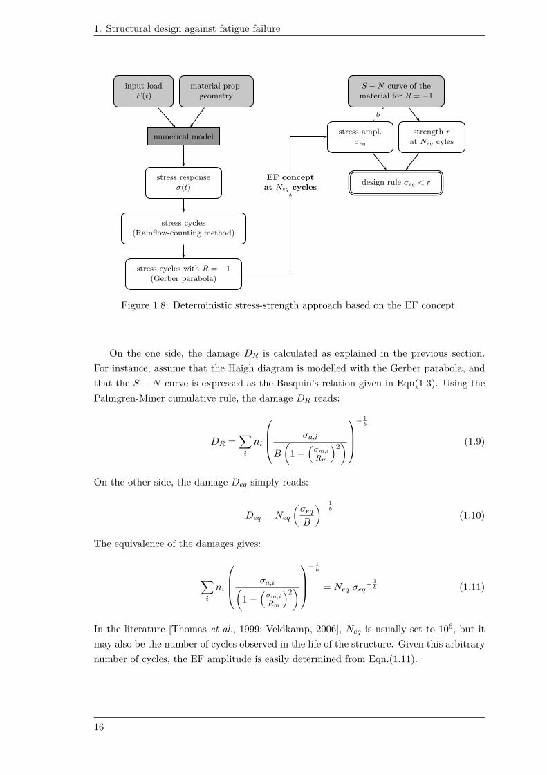
1.2.5 Equivalent fatigue concept
In industry, fatigue design codes can also be deterministic stress-strength approaches as
illustrated in Figure 1.8. The history σ(t) of the stress response is summarized into a
single stress value which is then compared with a given fatigue strength. The Equivalent
Fatigue (EF) concept is commonly used to summarize the stress response. It converts a
VA signal σ(t) into a simple CA cycle which, repeated an arbitrary number of times Neq,
produces the same fatigue damage to the structure. This cycle is generally defined as fully
reversed in order to be wholly characterized by its amplitude σeq. This amplitude is then
compared with the fatigue strength r at Neq cycles which is derived from the S − N curve
of the material expressed for R = −1. The design rule thus becomes σeq < r. In this
section, the EF concept is first applied to an assumed VA stress response at the critical
location of the structure. It is then extended to a VA load imposed on the global structure
as is usually the case for pre-dimensioning and test characterization.
1.2.5.1 Equivalent fatigue stress response
The stress response of a structure to an input VA load is assumed to be uniaxial at the
critical location (or at least dominated by a direction). Its cycles are extracted, and the
ith one is characterized by a mean σm,i, an amplitude σa,i and a number of occurrences ni.
The damage induced by these cycles is denoted by DR. Let Deq be the damage produced
by the EF cycle repeated Neq times. Given an arbitrary Neq, the symmetric alternating
amplitude σeq must be determined so that DR = Deq.
15
1. Structural design against fatigue failure
input loadF (t)
material prop.geometry
S −N curve of thematerial for R = −1
numerical modelstress ampl.
σeq
strength r
at Neq cyles
stress responseσ(t)
EF concept
at Neq cyclesdesign rule σeq < r
stress cycles(Rainflow-counting method)
stress cycles with R = −1(Gerber parabola)
b
Figure 1.8: Deterministic stress-strength approach based on the EF concept.
On the one side, the damage DR is calculated as explained in the previous section.
For instance, assume that the Haigh diagram is modelled with the Gerber parabola, and
that the S − N curve is expressed as the Basquin’s relation given in Eqn(1.3). Using the
Palmgren-Miner cumulative rule, the damage DR reads:
DR =∑
i
ni
σa,i
B
(
1 −(
σm,i
Rm
)2)
− 1b
(1.9)
On the other side, the damage Deq simply reads:
Deq = Neq
(
σeq
B
)− 1b
(1.10)
The equivalence of the damages gives:
∑
i
ni
σa,i(
1 −(
σm,i
Rm
)2)
− 1b
= Neq σeq− 1
b (1.11)
In the literature [Thomas et al., 1999; Veldkamp, 2006], Neq is usually set to 106, but it
may also be the number of cycles observed in the life of the structure. Given this arbitrary
number of cycles, the EF amplitude is easily determined from Eqn.(1.11).
16

1.2. Deterministic fatigue design
1.2.5.2 Equivalent fatigue load
The fatigue design approaches introduced previously require the knowledge of the stress
response at the critical location of the structure. Often, in-service measurements provide
the input loads, and the stress response history σ(t) is derived from a time-demanding
evaluation of the numerical model. Under some assumptions, the EF concept may also be
used to summarize the load applied to the global structure instead of the stress response
[Thomas et al., 1999; Veldkamp, 2006; Genet, 2006]. In such a case, the EF cycle of the
load is applied to the numerical model, and the cycle of stress response thus obtained is
interpreted as being repeated Neq times. The EF load is an extremely convenient tool as it
avoids the time-demanding calculation of σ(t). Additionally, it presents a large potential
for other fatigue applications. For instance in Morel et al. [1993], the amplitude of the EF
cycle is derived from field measurements, and then used as a setting value on a testing
machine in order to perform simple but representative fatigue tests on real structures.
The amplitude of the EF cycle may also be employed to compare different loads as it is a
scalar representation of the load severity.
The equivalence of the damages DR and Deq must be assessed strictly from the loads
that are independent from the geometry of the structure. Assume that a force load F (t) is
applied to the structure. The ith force cycle is characterized by a mean Fm,i, an amplitude
Fa,i and a number of occurrences ni. Assume that the EF cycle is fully reversed, and
features an amplitude Feq. This amplitude must be determined so that DR = Deq. On
the hypothesis that the global behaviour of the structure is elastic and quasi-static [Genet,
2006], the stress response at the critical location is proportional to the applied force:
σ(t) = λ F (t) (1.12)
where λ depends on the structure’s geometry and material. This linear assumption is
acceptable in the case of a structure designed for high cycle fatigue, as macroscopic cyclic
plasticity is not observed. According to Eqn.(1.12), the following relations can be written:
σm = λ Fm
σa = λ Fa
σeq = λ Feq
(1.13)
and the Basquin’s relation becomes:
λ F ′a = B N b (1.14)
The damage Deq expressed from the force thus reads:
Deq = Neq
(
λ Feq
B
)− 1b
(1.15)
17

1. Structural design against fatigue failure
Concerning the damage DR, Eqn.(1.9) requires the knowledge of the tensile strength Rm.
The coefficient λ cannot be used to link the tensile strength to the ‘tensile force’ as
plasticity occurs. An approximation is therefore made by considering the ratio K of the
tensile strength to the stress at Neq cycles:
K =Rm
σeq=
Rm
λ Feq(1.16)
K depends on the fatigue behaviour of the material, and is commonly set to 2.5 for steels
when Neq = 106 cycles [Thomas et al., 1999]. The damage DR then reads:
DR =∑
i
ni
λ Fa,i
B
(
1 −(
Fm,i
K Feq
)2)
− 1b
(1.17)
The equivalence of damages becomes:
∑
i
ni
Fa,i(
1 −(
Fm,i
K Feq
)2)
− 1b
= Neq Feq− 1
b (1.18)
λ and B are removed by expressing the equivalence, therefore, the structure’s geometry
is not involved in the expression of the EF amplitude. Feq is assessed numerically using
Newton’s method to find the root of the following function f(Feq):
f(Feq) = 1 − Feq1b
Neq
∑
i
ni
Fa,i(
1 −(
Fm,i
K Feq
)2)
− 1b
(1.19)
The function f(Feq) is not defined for Feq = Fm,i/K. It is recommended to set the initial
point F(0)eq of Newton’s method so that F
(0)eq > maxi(Fm,i/K).
1.2.6 Fatigue design codes in industry
The fatigue behaviour of structures is strongly affected by uncertainties [Svensson, 1997].
Tovo [2001] sorts these uncertainties into two fundamentally different categories that are:
• the inherent uncertainties of the material properties, loads, geometry and fatigue
behaviour.
• the errors of the numerical model as well as in the estimation of the parameters.
The first category is the aleatoric uncertainties. They correspond to the parameters en-
tering into mechanical modelling that are intrinsically random. The second category rep-
18

1.3. Probabilistic fatigue design
resents the epistemic uncertainties. In fatigue, they are caused by a lack of knowledge in
the complex damage mechanism or by the shortage of experimental data. In contrast to
the aleatoric uncertainties, they can, in principle, be reduced.
Most structures are designed against fatigue with deterministic approaches that are
either codified in standards or based on practical experience. These approaches imply
the use of so-called safety factors in an attempt to ensure the integrity of the structure
while covering the inherent uncertainties mentioned above. Such factors are based on the
know-how acquired through experience feedback, and are consequently highly subjective.
In industry, two main fatigue design approaches exist:
• The first one is the application of the flowchart depicted in Figure 1.5 with safety
rules. A codified load history is imposed on the structure, and the fraction of damage
is calculated for each stress response cycle with a pessimistic S − N curve. This
curve can either be the isoprobabilistic S − N curve representing the median shifted
down by uf (e.g. 3) standard deviations, or the most conservative curve obtained
when multiplying the median one by a factor reducing the fatigue life and a factor
augmenting the stress level [AFCEN, 2000].
• The second approach refers to the deterministic stress-strength approach. A design
load representing the severity of the in-service loads is applied to the numerical
model, and its stress response is compared to a conservative fatigue strength. Such
a procedure may be grounded upon the EF concept as depicted in Figure 1.8.
For illustrations of such design approaches and safety factors, the reader is referred to codes
such as the RCC-M standard [AFCEN, 2000] for nuclear applications, or the FEM1.001
[FEM, 1998] for lifting machines.
1.3 Probabilistic fatigue design
1.3.1 Introduction
As mentioned previously, safety factors are applied in deterministic fatigue design ap-
proaches to cover the uncertainties that are inherent to the fatigue phenomenon. Although
these approaches mostly give satisfactory results, the use of safety factors often leads to
over-design, i.e. excessive dimensions and masses. Within the scope of cost optimization,
engineers are asked to design structures that are safe while using a minimum quantity
of raw materials. Such a challenge can only be met through a better understanding of
the structural behaviour. From this perspective, the knowledge of the safety margin and
the most influent design factors on structural reliability is valuable for the design process.
Deterministic methods are not sufficient to acquire this information, and probabilistic
approaches are gradually finding their way into industrial research in order to provide
answers to these recent expectations.
19

1. Structural design against fatigue failure
This part is devoted to these approaches. Section 1.3.2 explains the principles of the
probabilistic approaches. Section 1.3.3 presents tools for inferring statistical distributions.
Section 1.3.4 discusses methods for modelling the uncertainty of the in-service loads. Sec-
tion 1.3.5 introduces the probabilistic S − N curves to model the scatter of the fatigue
behaviour. Section 1.3.6 explains the probabilistic Stress-stRength approach developed
by Thomas et al. [1999]. Finally, Section 1.3.7 presents the approach implemented in the
APPRoFi project.
1.3.2 Principles of the probabilistic approaches
In mechanics, probabilistic approaches are a way to consider the physical uncertainties
affecting a structure [Ditlevsen and Madsen, 1996; Lemaire, 2009]. With such approaches,
each parameter entering into mechanical modelling (e.g. structure dimensions, bound-
ary conditions, material properties, fatigue behaviour...) is no longer a single value or
number but a random variable. The mechanical response then becomes random, and its
uncertainty can be quantified.
The present section is based on Lemaire [2009] and Sudret [2011]. Figure 1.9 depicts
the general flowchart of a probabilistic approach. At first, a deterministic model M(Step 1) must be defined, and particularly its input parameters x and its response y. As
mentioned above, the vector x is composed of the geometry, load and material parameters.
In fatigue design, the response y may for instance be a damage value, a stress level or a
number of cycles to failure.
Step 2 of the probabilistic approach is the stochastic modelling of uncertainties.
The variabilities of x are modelled with Probability Density Functions (PDF) such as
Gaussian, Weibull, uniform... The parameters are now random variables X = X(ω)†. In
practice, the PDFs are inferred from data sets that may be acquired by:
• quality controls for the geometry parameters.
• experience feedback and field measurements for the uncertainty of the in-service
loads.
• multiple tests on structures and specimens for material properties and fatigue beha-
viour.
Classically, the parameters of the PDFs are adjusted by maximum likelihood estimation,
and goodness-of-fit tests are conducted to determine whether the assumed distribution is
valid (see Section 1.3.3 for further details on these statistical inference methods). Bayesian
inference may also be used when the size of the data set is small and when there is a priori
†In this thesis, random parameters are written in capital letters. However, ω is sometimes used to
underline the random nature of the quantity. For instance, the random stress level and the random
number of cycles to failure are denoted by σ(ω) and N(ω) respectively.
20

1.3. Probabilistic fatigue design
information. It consists in determining a ‘posterior’ distribution according to the Bayes’
rule, given a ‘prior’ believed distribution and the observation of data. Finally, when
no data are available, recourse to expert judgement is required. A distribution and its
parameters are simply assumed based on empirical knowledge.
Step 3 is the propagation of uncertainty. The response of the deterministic model is
now a random variable Y = M(X) whose realizations are only known when evaluating Mfor a given realization x of X. The propagation of uncertainty aims at characterizing the
random response Y . Different analyses exist depending on the objective of the study. In
the frame of this thesis, a structural reliability analysis is conducted. In such an analysis, a
failure scenario of the structure is mathematically represented by a performance function
G(X) (or several) which is defined in order to give positive values in the safe domain
and zero or negative values in the failure domain. The objective of the analysis is then
to determine the failure probability Pf = Prob(G(X) ≤ 0) through the use of reliability
methods that are further discussed in Chapter 2. Note that the analysis also produces the
importance factors or sensitivity indices which quantify the influence of the random input
parameters on structural reliability. Finally, in the case of fatigue design, the performance
function G can either be the difference between 1 and the cumulated damage, the difference
between a fatigue strength and a stress level, or the difference between a reference number
of cycles and the number of cycles to failure.
Step 2stochasticmodelling
Step 1deterministic
model M
Step 3propagation of
uncertainty
random inputparameters: X
modelM
characterization ofthe random response Y
(reliability analysis orsensitivity analysis)
Figure 1.9: Steps of the probabilistic approach in mechanics.
1.3.3 Basic statistical inference methods
This section introduces some basic methods that are employed in this research work for
modelling the uncertainty of the input parameters.
1.3.3.1 Maximum likelihood estimation
Statistical modelling aims at determining the stochastic model shared by a set of observa-
tions x(1), . . . , x(Q) which are presumed to be independent and identically distributed.
21

1. Structural design against fatigue failure
To establish such a model, two types of methods exist in the literature: parametric methods
and non-parametric methods. Within a parametric framework, a statistical distribution
is assumed, and its parameters are inferred according to the observations. Conversely,
non-parametric methods such as kernel density estimation [Saporta, 2006] do not rely
on assumptions that the data are drawn from a given distribution. In the frame of this
thesis, a parametric method known as Maximum Likelihood (ML) estimation [Fisher,
1950] is used.
Assume fX to be the PDF of the random variable X whose available observations
are denoted by x(1), . . . , x(Q). ML estimation aims at determining the parameters θ =
θ1, . . . , θh of fX according to the observations. For this purpose, the likelihood L is
expressed as:
L(
θ; x(1), . . . , x(Q))
=Q∏
i=1
fX
(
x(i); θ)
(1.20)
The ML estimate θ corresponds to the value of θ that maximizes the likelihood. In
practice, the log-likelihood is used in order to determine θ. The optimization problem to
solve then reads:
θ = arg minQ∑
i=1
− ln fX
(
x(i); θ)
(1.21)
In some cases, an explicit expression of the ML estimate may be derived. However, the
optimization problem must often be solved numerically.
The selection of a PDF from a set of candidate models is done thanks to likelihood
criteria such as AIC (Akaike Information Criterion) [Akaike, 1974] and BIC (Bayesian
Information Criterion) [Schwarz, 1978]. These criteria measure the relative goodness of
fit of models, and are based on the maximum value Lmax of the likelihood attained at θ.
AIC reads:
AIC = −2 ln Lmax + 2 h (1.22)
where h denotes the number of components of θ. BIC reads:
BIC = −2 ln Lmax + h ln Q (1.23)
where Q is recalled to be the number of available observations. The model to select is the
one with the minimum AIC and BIC values. However, these criteria do not tell how well
a model fits the data in an absolute sense. They can in fact only be used for comparing
different models, and analysis must then be completed with goodness-of-fit tests to validate
model hypotheses. These tests are introduced in the next section.
22

1.3. Probabilistic fatigue design
1.3.3.2 Goodness-of-fit tests
Goodness-Of-Fit (GOF) tests check whether there is evidence that a set of observations
does not arise from a given statistical distribution. The null hypothesis usually denoted by
H0 corresponds to the position where the observations arise from the assumed distribution.
Conversely, the alternative hypothesis H1 is the position where the observations are not
drawn from the assumed distribution. Let F0 be the Cumulative Distribution Function
(CDF) that is assumed, and FQ be the empirical CDF of the observations. GOF tests
quantify a distance between FQ and F0 known as the test statistic which is then compared
with a critical value, in order to determine whether H0 should be rejected or not (note
that H0 can never be proven). This critical value is associated with a significance level
which corresponds to the probability of making an error by rejecting H0. This probability
is usually set to 5%. Another way of using GOF tests is to use the p-value in order to
examine the strength of evidence that the set of observations provides against H0. The
p-value represents the probability of obtaining a test statistic at least as extreme as the
value observed, assuming that H0 is true. Hence the smaller the p-value, the stronger the
evidence against H0. Often, H0 is rejected when the p-value is below the significance level.
The first GOF test considered in this research work is Kolmogorov-Smirnov’s. Its
statistic D reads:
D = maxi∈1,...,Q
[
|F0(x(i)) − FQ(x(i))|, |F0(x(i)) − FQ(x(i−1))|]
(1.24)
Under H0, this statistic is asymptotically (Q → +∞) distributed as [Saporta, 2006]:
Prob(√
QD > d) → K(d) =+∞∑
k=−∞(−1)k exp(−2k2d2) (1.25)
H0 is then rejected if√
QD is higher than a critical value dα (see Saporta [2006] for tables
of dα depending on the significance level).
The Anderson-Darling test [NIST/SEMATECH] is an alternative to the Kolmogorov-
Smirnov test, and is often preferred for its ability to give more weight to the distribution
tails. Its statistic A reads:
A = −Q −Q∑
i=1
2i − 1
Q
(
ln(F0(x(i))) + ln(1 − F0(x(Q−i+1))))
(1.26)
Contrary to the Kolmogorov-Smirnov test, the critical values of the Anderson-Darling test
depend on the distribution which is assumed (see D’Agostino and Stephens [1986] for tables
of critical values). The asymptotic distribution of the Anderson-Darling statistic presents
a complex expression (see Marsaglia and Marsaglia [2004]). The calculation of the p-value
is therefore relatively difficult, but one may use the package ‘ADGofTest’ [Gil Bellosta,
23

1. Structural design against fatigue failure
2011] of the programming language R which provides the p-value calculation based on the
works by Marsaglia and Marsaglia [2004].
1.3.4 Modelling of in-service loads
The uncertainty of the in-service loads must be considered in the fatigue calculation so
as to determine a correct structural design. Field measurements are generally conducted
to examine this uncertainty. The problem tackled in this section is the determination of
a stochastic model that matches the variability observed in a database of measurements.
A load mix strategy dividing load histories into elementary life situations and the use of
mixture models to represent Rainflow matrices are discussed here. It is important to note
that this section is restricted to the methods studied in the frame of the APPRoFi project.
Approaches such as the modelling of loads with stationary Gaussian processes [Pitoiset,
2001; Benasciutti and Tovo, 2005] or Markovian processes [Mattrand and Bourinet, 2011;
Mattrand, 2011] are possible alternatives.
1.3.4.1 Load mix strategy
The load mix strategy [Thomas et al., 1999; Bignonnet et al., 2009; Lefebvre et al., 2009]
considers that in-service loads are mixtures of elementary life situations corresponding to
specific usages of the structure. An elementary situation features:
• field measurements of the corresponding load which are generally converted into
Rainflow matrices.
• a random percentage of occurrence during the structure’s life span. Such informa-
tion may be extracted from a customer survey or from field measurements of some
parameters in addition to the load.
Table 1.1 presents the load mix strategy as described by Bignonnet et al. [2009]. Q1 and
Q2 are quantities characterizing the structure’s usage (e.g. the carried mass and speed).
Two classes denoted by Qi1 and Qi
2 are defined for each quantity Qi (e.g. the class ≤ 500
kg and the class > 500 kg for the carried mass, or ≤ 100 km/h and > 100 km/h for
the speed). Four elementary life situations then exist: (Q11, Q2
1), (Q11, Q2
2), (Q12, Q2
1) and
(Q12, Q2
2). Several Rainflow matrices M(1)j,k , M
(2)j,k ,... representing the applied loads during
realizations of the situation (Q1j , Q2
k) are derived from field measurements. Note that these
Rainflow matrices are normalized to a given reference (e.g. 1 second or 1 km) in order
to facilitate further use. For each class Qij , the ratio of the time spent in this class to
the structure’s life span is modelled with a random percentage of occurrence P ij which is
usually considered as uniform [Lefebvre et al., 2009]. A Rainflow matrix L representing
a virtual life of the structure is generated by selecting a realization p11, p1
2, p21, p2
2 of the
24
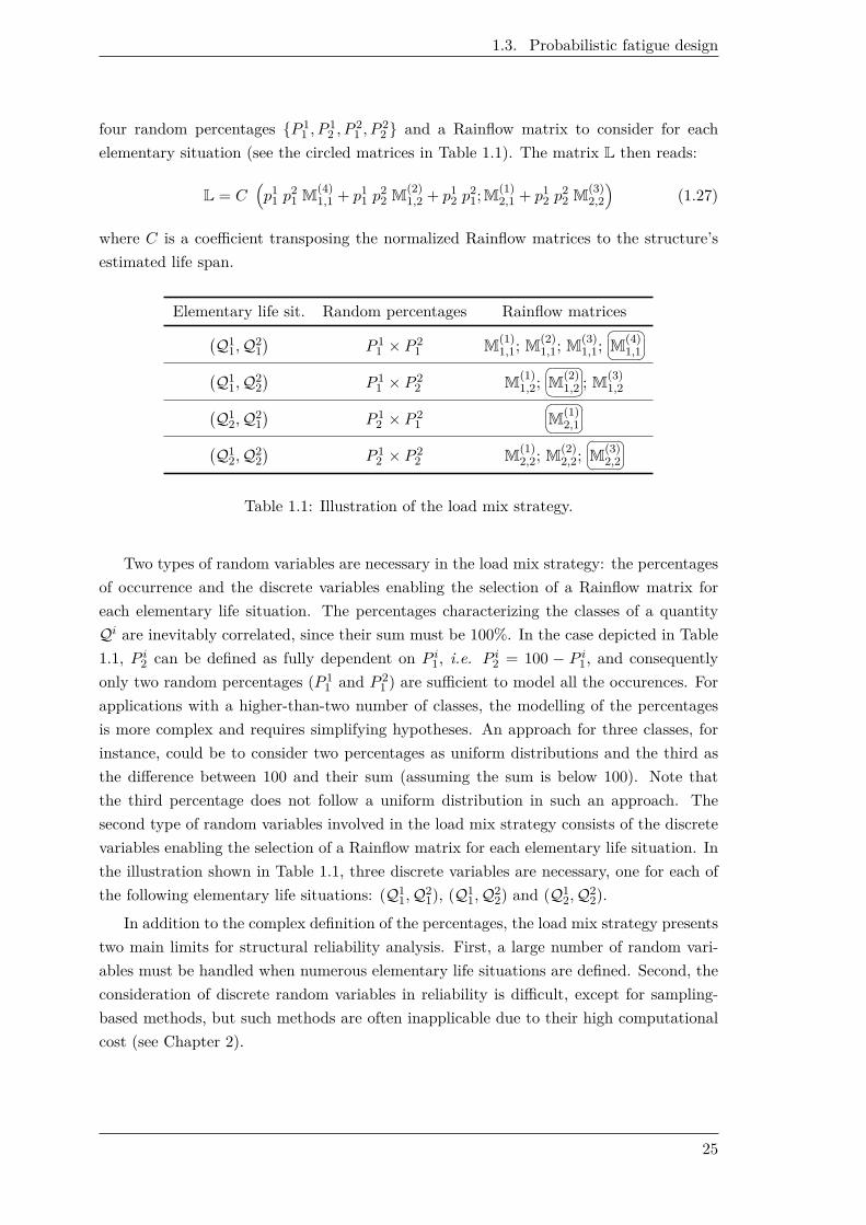
1.3. Probabilistic fatigue design
four random percentages P 11 , P 1
2 , P 21 , P 2
2 and a Rainflow matrix to consider for each
elementary situation (see the circled matrices in Table 1.1). The matrix L then reads:
L = C(
p11 p2
1 M(4)1,1 + p1
1 p22 M
(2)1,2 + p1
2 p21;M
(1)2,1 + p1
2 p22 M
(3)2,2
)
(1.27)
where C is a coefficient transposing the normalized Rainflow matrices to the structure’s
estimated life span.
Elementary life sit. Random percentages Rainflow matrices
(Q11, Q2
1
)
P 11 × P 2
1 M(1)1,1; M
(2)1,1; M
(3)1,1;
M
(4)1,1
(Q11, Q2
2
)
P 11 × P 2
2 M(1)1,2;
M
(2)1,2 ; M
(3)1,2
(Q12, Q2
1
)
P 12 × P 2
1
M
(1)2,1
(Q12, Q2
2
)
P 12 × P 2
2 M(1)2,2; M
(2)2,2;
M
(3)2,2
Table 1.1: Illustration of the load mix strategy.
Two types of random variables are necessary in the load mix strategy: the percentages
of occurrence and the discrete variables enabling the selection of a Rainflow matrix for
each elementary life situation. The percentages characterizing the classes of a quantity
Qi are inevitably correlated, since their sum must be 100%. In the case depicted in Table
1.1, P i2 can be defined as fully dependent on P i
1, i.e. P i2 = 100 − P i
1, and consequently
only two random percentages (P 11 and P 2
1 ) are sufficient to model all the occurences. For
applications with a higher-than-two number of classes, the modelling of the percentages
is more complex and requires simplifying hypotheses. An approach for three classes, for
instance, could be to consider two percentages as uniform distributions and the third as
the difference between 100 and their sum (assuming the sum is below 100). Note that
the third percentage does not follow a uniform distribution in such an approach. The
second type of random variables involved in the load mix strategy consists of the discrete
variables enabling the selection of a Rainflow matrix for each elementary life situation. In
the illustration shown in Table 1.1, three discrete variables are necessary, one for each of
the following elementary life situations: (Q11, Q2
1), (Q11, Q2
2) and (Q12, Q2
2).
In addition to the complex definition of the percentages, the load mix strategy presents
two main limits for structural reliability analysis. First, a large number of random vari-
ables must be handled when numerous elementary life situations are defined. Second, the
consideration of discrete random variables in reliability is difficult, except for sampling-
based methods, but such methods are often inapplicable due to their high computational
cost (see Chapter 2).
25

1. Structural design against fatigue failure
1.3.4.2 Mixture models of Rainflow matrices
Field measurements are generally conducted in a short period of time, and consequently,
all the cycles the structure may undergo during its life are not observed. The parametric
modelling of Rainflow matrices with unimodal joint PDFs is a solution to extrapolate more
damaging cycles. Nevertheless, Rainflow matrices are multimodal when load histories are
non-stationary random processes, and a simple joint PDF is thus not always sufficient
[Nagode et al., 2001]. This section introduces the concept of mixture models for the
particular case of Rainflow matrices, and is mainly based on the works by Nagode and
Fajdiga [1998, 2000, 2006]; Nagode et al. [2001]; Nagode [2012]. Note that after Nagode
et al. [2001], Rainflow matrices are considered in this section as representations of the
number of cycles ordered by mean σm and range ∆σ (instead of amplitude).
For convenience, let S be the random vector Sm, Srt = σm(ω), ∆σ(ω)t where
Sm = σm(ω) is the random mean and Sr = ∆σ(ω) is the random range. A realization of
this random vector is denoted by s = σm, ∆σt. A Rainflow matrix can be defined as a
weighted sum of component distributions:
fS(s; w, θ(1), . . . , θ(z)) =z∑
l=1
w(l) f(l)S
(s; θ(l)) (1.28)
where θ(l) are the parameters of the lth component distribution f(l)S
(s; θ(l)), and where
the mixing weights are denoted by w = w(1), . . . , w(z)t with w(l) ≥ 0 for l = 1, . . . , z
and∑z
l=1 w(l) = 1. The component distributions are presumed as being conditionally
independent. Hence, f(l)S
(s; θ(l)) reads:
f(l)S
(s; θ(l)) = f(l)Sm
(σm; θ(l)Sm
) × f(l)Sr
(∆σ; θ(l)Sr
) (1.29)
where f(l)Sm
(σm; θ(l)Sm
) denotes the distribution of the random mean and f(l)Sr
(∆σ; θ(l)Sr
) the
distribution of the random range for the lth component.
Nagode et al. [2001] propose mixture models composed of Gaussian distributions for
means and two-parameter Weibull distributions for ranges. An illustration of such mixture
models is depicted in Figure 1.10. The Gaussian distribution of means corresponding to
the lth component reads:
f(l)Sm
(σm; θ(l)Sm
) =1
√2πσ
(l)Sm
exp
−1
2
(
σm − µ(l)Sm
)2
σ(l)Sm
2
(1.30)
where θ(l)Sm
is the vector containing the mean µ(l)Sm
and the standard deviation σ(l)Sm
of the
random mean Sm for the lth component. Ranges are modelled with Weibull distributions
because the PDF support is R+. The Weibull distribution of ranges corresponding to the
26

1.3. Probabilistic fatigue design
lth component reads:
f(l)Sr
(∆σ; θ(l)Sr
) =h
(l)Sr
λ(l)Sr
∆σ
λ(l)Sr
κ(l)Sr
−1
exp
−
∆σ
λ(l)Sr
κ(l)Sr
(1.31)
where θ(l)Sr
is the vector containing the shape parameter κ(l)Sr
and the scale parameter λ(l)Sr
of the random range Sr for the lth component. As expressed in Eqn.(1.29), Sm and
Sr corresponding to the lth component stand for independent variables. However, it is
underlined by Nagode et al. [2001] that a global correlation between mean and range can
be modelled by selecting an appropriate number of component distributions.
Figure 1.10: Illustration of a mixture model from Nagode et al. [2001]. The black dotsrepresent the cycles. The mixture model contains five component distributions.
In order to establish a mixture model, the number of component distributions z, the
mixing weights w and the parameters θ(l), l = 1, . . . , z have to be determined. Such
an analysis may be conducted with the REBMIX algorithm [Nagode and Fajdiga, 1998,
2000, 2006; Nagode et al., 2001]. Note that the R package called ‘rebmix’ [Nagode and Fa-
jdiga, 2011a,b] provides an implementation of the algorithm whose principles are presented
below. The reader is referred to Nagode [2012] for further details.
Principles of the REBMIX algorithm
For the sake of clarity, the algorithm, depicted in Figure 1.11, is described on a simple
one-dimensional Rainflow matrix, i.e. a histogram into which n fully reversed (mean = 0)
stress cycles are sorted according to the range. In the general case of a Rainflow matrix
ordered by mean and range, the procedure is similar.
27

1. Structural design against fatigue failure
(a) Determination of the global mode for thefirst component distribution (l = 1).
(b) Identification of the n(1) cycles (in grey) be-longing to the first component distribution usingthe iterative clustering procedure and the roughestimation of the component parameters.
(c) Inference of the distribution’s parameters us-ing ML estimation.
(d) Determination of the global mode for thesecond component distribution (l = 2).
(e) Identification of the n(2) cycles (in grey) be-longing to the second component distributionand inference of the distribution’s parameters.
(f) Mixture model. The final residue is assignedto the second component distribution accordingto the Bayes decision rule.
Figure 1.11: Bases of the REBMIX algorithm after Nagode and Fajdiga [2006].
28

1.3. Probabilistic fatigue design
For this simplified study, the objective is to define the one-dimensional Rainflow matrix
ordered by range as a weighted sum of component distributions:
fSr (∆σ; w, θ(1)Sr
, . . . , θ(z)Sr
) =z∑
l=1
w(l) f(l)Sr
(∆σ; θ(l)Sr
) (1.32)
Let the range axis be discretized into classes ∆σk of width br. The centre of the bin ∆σk is
denoted by ∆σk. The number of cycles falling into the bin ∆σk is nk, and the corresponding
relative frequency reads fk = nk/n. The number of cycles belonging to the lth component
distribution is n(l). The number of cycles of the lth component falling into the bin ∆σk
is denoted by n(l)k , and the corresponding relative frequency reads f
(l)k = n
(l)k /n(l). The
mixing weight w(l) associated with the lth component is calculated as:
w(l) =n(l)
n(1.33)
Initially, l is set to 1, n(l)k to nk, n(l) to n, and f
(l)k to fk. The algorithm starts with the
determination of the global mode (see Figure 1.11(a)), i.e. the bin ∆σr(l) at which:
∆σr(l) = arg maxk
f(l)k (1.34)
This global mode characterizes the lth component distribution.
An iterative clustering procedure is then applied to determine the n(l) cycles be-
longing to the lth component distribution (see Figure 1.11(b)). The algorithm is provided
in Nagode [2012]. This procedure is based on the deviation e(l)k between n
(l)k and the
component frequency at ∆σk:
e(l)k = n
(l)k − f
(l)Sr
(∆σk; θ(l)Sr
) br n(l) (1.35)
The most deviating cycles are gradually transferred to the residue, and the mixing weight
w(l) is recalculated using the updated number n(l) in Eqn.(1.33). At the end of the
procedure, the residue is composed of the n cycles that do not belong to the lth component
distribution.
At each iteration of the clustering procedure, a rough estimation of the component
parameters θ(l)Sr
= κ(l)Sr
, λ(l)Sr
t enables the calculation of f(l)Sr
(∆σk; θ(l)Sr
) in Eqn.(1.35).
This rough estimation is based on the expression of constraints that prevent the component
distribution from moving away from its global mode. The first constraint ensures the
equivalence of the relative frequencies at the global mode:
f(l)Sr
(
∆σr(l) ; θ(l)Sr
)
br = f(l)
r(l) (1.36)
The second constraint makes the global mode of the component distribution coincide with
29
1. Structural design against fatigue failure
∆σr(l) :
∂f(l)Sr
(
∆σ; θ(l)Sr
)
∂∆σ
∣
∣
∣
∣
∣
∣
∆σr(l)
= 0 (1.37)
The parameters θ(l)Sr
are estimated using Eqns.(1.36) and (1.37). Note that in the case of
a Rainflow matrix ordered by mean and range, additional constraints are required. They
are obtained from the equivalences of the component conditional relative frequencies at
the global mode [Nagode and Fajdiga, 2006; Nagode, 2012].
Once the n(l) cycles belonging to the lth component distribution have been identified,
and the mixing weight w(l) has been calculated, ML estimation is applied in order to
refine the parameters of the component distribution (see Figure 1.11(c)). l is then set to
l +1, and the same method is conducted to determine the new lth component distribution
on the basis of the n(l) = n cycles of the residue (see Figure 1.11(d) and Figure 1.11(e)).
The algorithm is run until the weight n(l)/n is below a critical weight wmin which is
set to avoid over-fitting (see Figure 1.11(f)). When this stopping condition is met, the
remaining cycles are assigned to the existing components using the Bayes decision rule
[Nagode, 2012], and the mixing weights and component parameters are recalculated. Note
that the user may also set a maximum number of component distributions. The most
adequate mixture model according to criteria such as AIC and BIC can be determined by
repeating the procedure with various maximum numbers of component distributions.
The parametric modelling examined in this section provides a continuous description
of the Rainflow matrices which may for instance be used to improve the load mix strategy
explained in Section 1.3.4.1. Within such an enhanced strategy, the elementary life situ-
ations feature mixture models instead of discrete Rainflow matrices.
1.3.5 Probabilistic S − N curves
As mentioned previously, the fatigue behaviour of materials is highly subjected to uncer-
tainties. This section introduces the probabilistic S − N curves as a way to model the
scatter observed in a data set of fatigue tests. It focuses on the ESOPE model that is
codified in the standard A03-405 [AFNOR, 1991], as well as the works by Guédé [2005];
Guédé et al. [2007]; Perrin [2008]. The reader may also refer to Sudret [2011] for further
details on these models. In practice, a probabilistic S − N curve features:
• a deterministic model D (or D−1) characterizing the median trend as σ50% = D(N)
or N50% = D−1(σ). This model may, for instance, be the Basquin’s relation which is
recalled to read σ50% = B N b for a given number of cycles N , or N50% = (σ/B)1/b
for a given stress level σ.
• a statistical distribution to model the scatter around the median trend. Such a
distribution may, for instance, be Gaussian or lognormal, and its dispersion may
30

1.3. Probabilistic fatigue design
be represented by either a constant standard deviation or a constant coefficient of
variation at any N or σ.
Let E = (σ(i), N (i)), i = 1, . . . , Q be a data set of fatigue tests where σ(i) is the nominal
stress undergone by a specimen and N (i) the corresponding number of cycles to failure.
ESOPE and Guédé’s models are explained below.
1.3.5.1 ESOPE
The ESOPE model [AFNOR, 1991] depicted in Figure 1.12(a) is based on the works by
Bastenaire [1960]. Let F (σ, N) be the function characterizing the probability that the
specimen fails before N cycles under the stress level σ. At a given N , this function is
assumed to vary in σ as the CDF of a Gaussian random variable with mean µSN (N) and
standard deviation σSN (N). The mean µSN (N) corresponds to the deterministic model
D(N), and σSN (N) is supposed to be constant at any N , i.e. σSN (N) = σSN . As a result,
F (σ, N) reads:
F (σ, N) = Φ
(
σ − D(N)
σSN
)
(1.38)
where Φ is the standard Gaussian CDF (zero mean and unit variance). In the case of the
Basquin’s relation, F (σ, N) becomes:
F (σ, N) = Φ
(
σ − B N b
σSN
)
(1.39)
Given that F (σ, N) is the CDF of a Gaussian random variable, an isoprobability S − N
curve reads:
σ = B N b + uf σSN (1.40)
where uf is a realization of the standard Gaussian variable Uf which represents the random
isoprobability S − N curve.
The ESOPE model is characterized by the parameters θ = B, b, σSN t. As recom-
mended in the standard A03-405 [AFNOR, 1991], ML estimation is applied to estimate
these parameters according to the data set E. Let N(σ, ω) be the random number of cycles
to failure under a stress level σ. Its PDF fN (σ, N) reads:
fN (σ, N) =∂F (σ, N)
∂N(1.41)
The likelihood L is expressed as:
L (B, b, σSN ;E) =Q∏
i=1
fN
(
σ(i), N (i); B, b, σSN
)
(1.42)
The optimization problem consists in numerically finding the optimum θ = B, b, σSN t
31

1. Structural design against fatigue failure
that reads:
θ = arg minθ∈R3
(− ln L (B, b, σSN ;E)) (1.43)
The solution of such a problem strongly depends on the starting point of the optimization
procedure. In this research work, a two-step procedure is implemented. First, the least
squares method is applied to determine rough estimates of B and b. The standard deviation
σSN is estimated by calculating the distance between the curve obtained by the least
squares method and the observations of E. Second, the ML estimation is performed
thanks to a simulated annealing algorithm whose starting point is the solution of the least
squares method.
Once the ESOPE model is fully determined, the initial hypothesis on the statistical
distribution must be validated a posteriori. A GOF test is performed to check whether
there is evidence against:
Uf =σ − B N b
σSN∼ N (0, 1) (1.44)
where N (0, 1) is the Gaussian distribution of parameters 0 (mean) and 1 (variance).
Figure 1.12(b) depicts an alternative model called ESOPE 2 in this thesis. For this
model, the coefficient of variation δSN is supposed to be constant at any N (instead of the
standard deviation σSN ). The function F (σ, N) of ESOPE 2 then reads:
F (σ, N) = Φ
(
σ − B N b
δSN B N b
)
(1.45)
The isoprobability S − N curve becomes:
σ = (1 + uf δSN ) B N b (1.46)
It is important to note that given Eqn.(1.46), all the isoprobability S − N curves feature
the same Basquin’s slope b. Finally, the GOF test conducted a posteriori checks whether
there is evidence against:
Uf =σ − B N b
δSN B N b∼ N (0, 1) (1.47)
1.3.5.2 Guédé’s model
In ESOPE, the distribution of the number of cycles to failure N(σ, ω) under the stress level
σ is not explicit. Guédé [2005]; Guédé et al. [2007] propose an alternative to ESOPE which
consider ln N(σ, ω) as a Gaussian random variable with parameters µN (σ) and σN (σ).
The model is depicted in Figure 1.13. Assuming that the random variables ln N(σ, ω) at
different stress levels are perfectly correlated, a single standard Gaussian random variable
32

1.3. Probabilistic fatigue design
(a) ESOPE. (b) ESOPE 2.
Figure 1.12: ESOPE and ESOPE 2. The solid line represents the median curve (50% prob-ability to fail at the stress level σ given N cycles). The dashed lines are the isoprobabilityS − N curves defined at 2.5% and 97.5%, i.e. uf = ∓1.96.
Uf is sufficient to model the scatter as:
ln N(σ, ω) = µN (σ) + Uf σN (σ) (1.48)
The mean µN (σ) corresponds to the deterministic model D−1(σ). In the case of the
Basquin’s relation, it reads:
µN (σ) = A + a ln σ (1.49)
where a = 1/b and A = − ln(B)/b. The scatter in N is supposed to be correctly modelled
with a constant coefficient of variation δN at any stress level:
σN (σ) = δN µN (σ) (1.50)
As a result, ln N(σ, ω) becomes:
ln N(σ, ω) = µN (σ) (1 + Uf δN ) (1.51)
An isoprobability S − N curve is simply obtained by selecting a realization uf of the
standard Gaussian random variable Uf .
Guédé’s model features the parameters θ = A, a, δN t. The PDF fN (σ, N) of the
number of cycles to failure N(σ, ω) under the stress level σ is explicitly known as:
fN (σ, N) =1
δN (A + a ln σ)Nφ
(
ln N − (A + a ln σ)
δN (A + a ln σ)
)
(1.52)
where φ is the standard Gaussian PDF. ML estimation is applied to estimate the para-
33

1. Structural design against fatigue failure
meters of the model according to the data set E. The likelihood L is expressed as:
L (A, a, δN ;E) =Q∏
i=1
fN
(
σ(i), N (i); A, a, δN
)
(1.53)
Note that censored data, i.e. fatigue tests which have been stopped before failure, can be
considered in the ML estimation [Perrin, 2008; Sudret, 2011]. For a given censored test
(σ∗, N∗), the value of the PDF fN (σ∗, N∗; A, a, δN ) is replaced in the ML estimation with
1 − FN (σ∗, N∗; A, a, δN ) where FN is the CDF of N(σ, ω) that reads:
FN (σ∗, N∗; A, a, δN ) = Φ
(
ln N∗ − (A + a ln σ∗)
δN (A + a ln σ∗)
)
(1.54)
Finally, the GOF test conducted a posteriori checks whether there is evidence against:
Uf =ln N(σ, ω) − (A + a ln σ)
δN (A + a ln σ)∼ N (0, 1) (1.55)
Figure 1.13: Guédé’s model. The solid line represents the median curve (50% probabilityto fail at N cycles given the stress level σ). The dashed lines are the isoprobability S − Ncurves defined at 2.5% and 97.5%.
1.3.5.3 Selection of the most adequate model
Given that the models are determined using ML estimation, likelihood criteria AIC and
BIC are relevant means for model selection [Perrin, 2008]. Additionally, the GOF tests
provide p-values which can be used to rank the initial hypotheses of the models. The
combination of AIC, BIC and the p-value thus represents a helpful approach for selecting
the most adequate model.
34

1.3. Probabilistic fatigue design
1.3.6 Probabilistic Stress-stRength approach
1.3.6.1 Structural design calculation
The probabilistic Stress-stRength approach [Thomas et al., 1999; Bignonnet and Thomas,
2004] is an engineering tool for designing new structures against fatigue with a given reli-
ability objective (or targeted failure probability). It consists of comparing two statistical
distributions, namely S and R, the former modelling the uncertainty of the in-service
loads while the latter models the uncertainty in the mechanical properties of the structure
to design. These distributions are commonly called Stress for S and stRength for R. As
depicted in Figure 1.14, the aim of the approach is to ascertain the mean strength µR
which ensures a reliability objective P f , considering that the distribution S is known to
be characterized by a mean µS and a standard deviation σS and that the Strength R
presents an inherent scatter in the form of a coefficient of variation δR. It is important
to firstly outline that the probabilistic Stress-stRength approach was implemented in the
DEFFI project [Bignonnet and Lieurade, 2007; Bignonnet et al., 2009; Ferlin et al., 2009;
Lefebvre et al., 2009] which is mentioned in introduction of this thesis.
Figure 1.14: Potential stRength distributions depending on its inherent scatter δR, theStress distribution and the reliability objective.
Stress-Strength Interference analysis
In the probabilistic Stress-stRength approach, the failure scenario is mathematically rep-
resented by the performance function G given as follows:
G(R, S) = R − S (1.56)
Failure occurs when the performance function is negative, i.e. when S is larger than R as
illustrated in Figure 1.15. The failure probability Pf consequently reads:
Pf = Prob(G(R, S) ≤ 0) = Prob(R − S ≤ 0) (1.57)
35

1. Structural design against fatigue failure
Within the frame of the probabilistic Stress-stRength approach, the Stress-Strength In-
terference (SSI) analysis [Booker et al., 2001] is applied to assess this failure probability.
This very simple and convenient engineering tool assumes that both S and R are known
and independent PDFs. Consequently, the failure probability simply reads:
Pf =
∫ +∞
−∞fS(s)FR(s)ds (1.58)
where fS is the assumed PDF of S and FR is the assumed CDF of R. The failure prob-
ability may be calculated using any numerical integration technique, but in some cases,
analytical expressions are directly available [Lemaire, 2009]. For instance, on the hypo-
thesis that S and R are Gaussian distributions, the failure probability becomes:
Pf = Φ
− µR − µS√
σ2R + σ2
S
(1.59)
where σR is the standard deviation of R. Thomas et al. [1999] mention that S may either
be a Gaussian, lognormal or Weibull distribution, whereas R is Gaussian given that it is
a combination of many variables (see the following paragraph on stRength distribution).
The next step is the capitalization of available data in order to determine the parameters
of the distributions S and R.
Figure 1.15: Stress-Strength Interference analysis. The dark area depicts the failure events.
Stress distribution
Figure 1.16 illustrates the general procedure for modelling the uncertainty of the in-service
loads. Beforehand, field measurements are conducted to obtain representative histories of
the different loads imposed on the structure. Let us assume that these recordings are force
histories F (t), but they can be defined in any other load quantity, e.g. in terms of displace-
36

1.3. Probabilistic fatigue design
ment. On the basis of these force histories, modelling techniques such as those detailed in
Section 1.3.4 are applied to model the uncertainties with random load parameters Xl (e.g.
random percentages of occurrence). By drawing a realization xl of these random para-
meters, a virtual load is generated. The damage contribution (or severity) of this virtual
load is then summarized into an EF cycle of amplitude Feq(xl, b, Neq) repeated Neq times.
Numerous realizations of the random parameters are drawn, and a large number of Feq
values is thus obtained. The distribution S modelling the variability of Feq is considered
in this section as Gaussian, because such an assumption provides an analytical expression
of the failure probability when combined with a Gaussian stRength (see Eqn.(1.59)).
uncertainty of in-service loads
field measurements F (t)
random load parameters Xl
xl
virtual load
Basquin’s
slope bEF cycle Feq(xl, b, Neq)
distribution S in Feq
S ∼ N (µS , σ2S)
Figure 1.16: Definition of the Stress distribution S.
StRength distribution
The stRength R represents the uncertainty of the mechanical properties (material proper-
ties, fabrication process) having fatigue damage consequences for the structure to design.
To enable a comparison with S, R is defined as the distribution of the fatigue strength
in force at Neq cycles. The objective here is to determine the coefficient of variation
δR = σR/µR interpreting the relative scatter of the fabrication process and its fatigue
damage consequences. Remember that the designer’s final aim is to set µR, given the
inherent scatter of R, the distribution S and the reliability objective P f . The general
37

1. Structural design against fatigue failure
procedure to determine R and the coefficient δR is depicted in Figure 1.17. Fatigue tests
performed on specimens and on structures which are similar to the one being designed are
collected in order to provide sufficient knowledge. On a stRength−N diagram, the data
sets at different numbers of cycles are combined into one group at Neq cycles following
the concept of Equivalent Fatigue strength (EF strength) [Hanaki et al., 2010] depicted
in Figure 1.18. The empirical mean mR and the unbiased estimate s∗R of the standard
deviation are then calculated from the group at Neq cycles. Given that the number Nt
of tested samples is usually small, the confidence in the stRength distribution R may be
weak. Thomas et al. [1999] consider that an acceptable mean value can be estimated with
Nt ≥ 8 samples: µR = mR. Assuming that R is a Gaussian random variable and that
µR = mR, the standard deviation is set as the upper bound of the confidence interval
defined by the risk γ:
σγ,Nt
R = s∗R
√
Nt − 1
kNt−1;γ/2(1.60)
where kNt−1;γ is the χ2 quantile. The quantity of interest, i.e. δγ,Nt
R , is derived from the
standard deviation and the mean. The distribution R is thus characterized only by δγ,Nt
R .
As mentioned previously, R is always considered as Gaussian.
uncertainty in the mechanical properties of thestructure to design (material, fabrication process)
data sets of fatigue tests forspecimens and similar structures
EF strength concept atNeq cycles
mR and s∗R at Neq cycles
µR and σNt,γR at Neq cycles
R ∼ N (δγ,Nt
R )
Figure 1.17: Definition of the stRength distribution R.
Risk analysis
An EF cycle of reference is arbitrarily selected in the distribution S (see Figure 1.19). Its
38

1.3. Probabilistic fatigue design
Figure 1.18: Concept of Equivalent Fatigue strength. The black dots represent the avail-able data set of fatigue tests. These samples at different numbers of cycles are projectedto Neq cycles, parallel to the median S − N curve of the material. The group of grey dotsis thus obtained, and the empirical mean mR and unbiased estimate s∗
R of the standarddeviation can be calculated at Neq.
amplitude is denoted by Fn, and its severity is defined as the positive α quantile:
Fn = µS + α σS (1.61)
The probability of exceeding Fn is then:
Prob(s > Fn) = 1 − Φ
(
Fn − µS
σS
)
= Φ(−α) (1.62)
Typical probabilities are 10−2, 10−3, 5 × 10⁻⁴. Fn represents neither a certain type of
situation nor the most severe observed load. It is an arbitrary amplitude that enables the
conversion of the failure probability calculation into a simple specification procedure. Fn
is associated with an acceptance criterion in stRength defined at κ standard deviations
below the mean stRength (see Figure 1.19):
µR = Fn + κσγ,Nt
R (1.63)
The relative mean strength m∗R is defined as:
m∗R =
µR
Fn=
1
1 − κδγ,Nt
R
(1.64)
39

1. Structural design against fatigue failure
S and R are recalled to be Gaussian distributions. By introducing Fn and the coefficient
of variation δS of S in Eqn.(1.59), the targeted failure probability P f can be rewritten as:
P f = Φ
− µR − µS√
(
µR δγ,Nt
R
)2+ (µS δS)2
Fn
Fn
(1.65)
It is then recast as:
P f = Φ
−m∗
R − 11+α δS
√
(
m∗R δγ,Nt
R
)2+(
δS
1+α δS
)2
(1.66)
In Eqn.(1.66), the parameters α, δS , δγ,Nt
R are known. The relative mean strength m∗R can
thus be assessed for a given reliability objective P f .
Figure 1.19: Reference EF cycle defined by Fn.
Figure 1.20 depicts an example of the structural design calculation from the designer’s
point of view. In practice, the reference EF cycle with amplitude Fn is applied to the
numerical model. In this illustration, the numerical model output used for fatigue cal-
culation is assumed to be the maximum principal stress σI at the critical location. The
designer checks that the point (Neq, σI) is below the isoprobability S − N curve of the
material that corresponds to the median curve shifted down by κ standard deviations (κ
determined using Eqn.(1.64)). In this example, the failure probability is below P f as the
gap is positive.
Conclusion
The probabilistic Stress-stRength approach detailed in this section is particularly well
adapted for industrial applications in the field of high cycle fatigue with linear mechanical
behaviour. Under some assumptions, it enables new structures to be designed with a given
40

1.3. Probabilistic fatigue design
Figure 1.20: Illustration of the structural design calculation. The numerical model is fromRelun [2011].
reliability objective. The probabilistic Stress-stRength approach consists of comparing the
distributions S and R that respectively model the uncertainty of the in-service loads and
the uncertainties in the mechanical properties of the structure to design. On the one
hand, S is characterized by a mean and a standard deviation, and on the other, R features
an inherent scatter in the form of its coefficient of variation. SSI analysis is applied in
order to provide an expression of the targeted failure probability which depends on the
distributions assumed for S and R (typically Gaussian). Finally, the mean strength µR
is determined by considering the inherent scatter of the stRength, the distribution S and
the reliability objective. In the frame of this thesis, the objective is not to ascertain the
optimum design of a new structure but to assess the failure probability of an already
designed structure. The adaption of the probabilistic Stress-stRength approach to this
case is explained in the next section.
1.3.6.2 Reliability assessment
Two adaptions of the probabilistic Stress-stRength approach to reliability assessment can
be devised depending on available data. The simplest alternative is formulated in terms
of a load quantity (e.g. in force). In such a case, S remains the distribution of the EF
amplitude Feq, but R is this time fully characterized by its parameters µR and σR which
are determined according to data sets of fatigue tests on the structure. Assumptions are
made on the distributions followed by S and R, and SSI analysis is applied to assess the
failure probability using Eqn.(1.58). Note that the numerical model of the structure is not
required in this adaption. However, the fatigue behaviour of the structure is often unknown
since conducting fatigue tests on a structure is usually unfeasible due to prohibitive costs or
41

1. Structural design against fatigue failure
structure size. It is then necessary to resort to the second adaption which simply requires
data sets of tests performed on smooth specimens in order to characterize the S −N curve
and other material properties. Note that experimental data on the structure’s geometry
may also be considered. The second adaption is depicted in Figure 1.21. Its different steps
are described in the following paragraphs.
random material
prop. and geometry
Xm, Xg
random load
parameters Xl
fatigue tests
on specimens
xm, xg xl
virtual load F (xl)
numerical modelEF cycle
Feq(xl, b, Neq)
cycle of stress response
σeq(xm,xg,xl, b, Neq)EF strength at
Neq cycles
Stress distribution S in σeq stRength distribution R
G = R− S
SSI analysis
Pf
b
Figure 1.21: Probabilistic Stress-stRength approach for reliability assessment.
Stress distribution
The uncertainties of the material properties, geometry and applied loads are statistically
modelled with the random vectors respectively denoted by Xm, Xg and Xl. The first
step of the procedure is the selection of a realization xm, xg, xl. A virtual load F (xl) is
generated with xl, and the corresponding EF cycle of amplitude Feq(xl, b, Neq) repeated
Neq times is calculated using the Basquin’s slope b of the S−N curve. The EF cycle is then
applied to the numerical model which depends on xm and xg. A cycle of stress response
42

1.3. Probabilistic fatigue design
is thus derived from the model evaluation. Assuming that the S − N curve is provided
for R = −1, this cycle is converted into its fully reversed equivalent whose amplitude
is σeq(xm, xg, xl, b, Neq). Several values of σeq are derived from the evaluation of the
numerical model for various realizations of the random variables. The observed dispersion
in σeq is modelled with a statistical distribution which corresponds to the Stress S.
stRength distribution
The uncertainty in the fatigue behaviour of the material is modelled with the stRength
distribution R. The EF strength concept presented in Section 1.3.6.1 is applied to determ-
ine the scatter of the fatigue strength at Neq cycles. As mentioned previously, a Gaussian
distribution is usually assumed for R [Lalanne, 2002].
SSI analysis
Given the distributions S and R, the failure probability is assessed using the SSI analysis,
and particularly Eqn.(1.58).
Limits
The application of the probabilistic Stress-stRength approach to reliability assessment
present two main limits. First, the influence of each random variable on structural reliab-
ility cannot be determined since Xm, Xg and Xl are gathered in S (remember that the
knowledge of the most influent variables represents a valuable information for the design
process). Second, the failure probability is extremely sensitive to the distribution that S
is assumed to follow. In this section, a simple example gives evidence of these two limits.
The beam case study illustrated in Figure 1.22 is subjected to a force F (t) in C.
Assuming that the structure remains in the elastic domain, the maximal stress in A reads:
σ(t) =F (t)
4(w v − v2)+
6 F (t) l w
w4 − (w − 2 v)4(1.67)
where v and w define the cross-section of the beam and l its length. σ(t) is supposed
to be the stress response used for fatigue calculation. In other words, Eqn.(1.67) is the
numerical model representing the mechanical behaviour of the case study.
The uncertainties of the geometry, force and fatigue behaviour of the material are
considered in this example. Table 1.2 reports the different random variables. The determ-
inistic parameters v, w and l are replaced with Gaussian variables V , W and L respectively.
The uncertainty of the force F is modelled with a simplified load mix strategy (see Section
1.3.4.1) involving only two elementary life situations. The most severe situation features
a Rainflow matrix M1 and a random percentage of occurrence P1 which is considered as
uniform in the interval [0; 60%]. The second situation is characterized by a Rainflow mat-
rix M2 and a random percentage P2 = 100−P1. The Rainflow matrices are modelled with
43

1. Structural design against fatigue failure
Figure 1.22: Characteristics of the beam case study.
independent joint Gaussian PDFs whose parameters are given in Table 1.3. The extreme
Rainflow matrices providing the number of cycles ordered by mean Fm and amplitude Fa
are depicted in Figure 1.23. Instead of sampling in the joint PDFs, the axes Fm and Fa
are arbitrarily discretized in order to represent the different cycles imposed on the struc-
ture. The number of occurrences of each cycle is obtained by reading the n axis which
corresponds to the value of the joint Gaussian PDF multiplied by a constant C (applied
to define a suitable life span). A virtual Rainflow matrix L(p1) representing a potential
service life of the structure is generated by drawing a realization p1 of P1:
L(p1) = p1 M1 + (1 − p1) M2 (1.68)
The virtual Rainflow matrix L(p1) is then summarized into an EF cycle of symmetric
alternating amplitude Feq(p1, b, Neq) repeated Neq = 106 times. Note that for the calcula-
tion of the EF cycle, the Basquin’s slope b is −0.3, and the ratio K of the tensile strength
to the stress at Neq = 106 cycles (see Eqn.(1.16)) is set to 2.5. Once determined, the EF
cycle is applied to the numerical model characterized by a selected geometry v, w, l. The
fully reversed cycle of the stress response in A is obtained using Eqn.(1.67). It features
an amplitude σeq(v, w, l, p1, b, Neq) and is interpreted as a cycle being repeated Neq = 106
times. Several values of σeq are calculated for various realizations of the random variables.
The dispersion observed is modelled with the distribution S which is then compared to
the distribution R of the EF strength at Neq = 106 cycles.
This case study is devised to be representative of the complex structures examined in
this thesis. A small failure probability (≈ 10−6) is thus defined, and the evaluation of
the numerical model, i.e. Eqn.(1.67), is considered as time-demanding. The latter condi-
tion limits the number of σeq values that can be evaluated in a practical amount of time,
therefore the Stress distribution must be determined with a relatively small number of
σeq values. In this study, three sets, each composed of only 100 σeq values, are considered
(see Figure 1.24). ML estimation is applied to determine the parameters of the Gaussian,
44

1.3. Probabilistic fatigue design
Variable Distribution Parameters
V (mm) Gaussian µV = 3; δV = 3%
W (mm) Gaussian µW = 50; δW = 3%
L (mm) Gaussian µL = 103; δL = 3%
P1 (%) Uniform [0; 60]
R (MPa) Gaussian µR = 180; δR = 10%
Table 1.2: Random variables of the beam case study.
Mean Std. dev.
M1Fm (N) 0 30
Fa (N) 700 50
M2Fm (N) 0 50
Fa (N) 250 50
Table 1.3: Parameters of the independent joint Gaussian PDFs of the Rainflow matricesM1 and M2.
lognormal and Weibull distributions fitting these sets. GOF tests are also conducted to
determine how well the assumed distributions fit the sets. The Anderson-Darling test is se-
lected since it gives more weight to the distribution tails where failure occurs. SSI analyses
are applied to assess the failure probability. The First Order Reliability Method (FORM)
is also applied to determine the influences of the Stress and stRength on structural reliabil-
ity (see Section 2.3.3.2). For this application, the elasticities of the Hasofer-Lind reliability
index β = −Φ−1(Pf ) with respect to the standard deviations σS and σR of the Stress and
stRength distributions are quantified. The elasticity value Eσimust be interpreted as
the percentage by which the Hasofer-Lind reliability index is increased when the standard
deviation of the ith random variable is raised by 1%.
Table 1.4 reports the results of the first set. The values of the likelihood criteria are
extremely similar, but the Gaussian distribution giving a failure probability of 4.9 × 10⁻⁶
seems the most adequate model according to its p-value. For the second set (see Table
1.5), the highest p-value is obtained for the Gaussian distribution, but the lognormal
distribution seems to be a relevant alternative according to AIC and BIC. The choice of the
distribution has a significant impact on the estimation of the failure probability, since Pf
is either 1.5×10⁻⁶ or 12×10−6. For the third set (see Table 1.6), the Weibull distribution
gives the best results, and the failure probability is 0.23 × 10⁻⁶. This study shows that
the accuracy of the probabilistic Stress-stRength approach for reliability assessment is
45

1. Structural design against fatigue failure
(a) Least severe matrix L(0). (b) Most severe matrix L(60).
Figure 1.23: Extreme Rainflow matrices obtained as mixtures of M1 and M2.
strongly affected by the number of model evaluations which can be performed in a practical
amount of time. In addition, confidence in the failure probability is extremely limited,
since the interference between Stress and stRength is at the extremes of the poorly known
distribution tails. For this case study, the order of magnitude of the failure probability
seems to be between 10−5 and 10−7, which represents a relatively wide interval. To finish,
it can be noted for this case study that the elasticities of the Hasofer-Lind reliability index
show that the standard deviation of the stRength has more impact on structural reliability
than the standard deviation of the Stress when the latter is modelled with a Gaussian or
Weibull distribution. An opposite behaviour is observed with a lognormal Stress.
Stress distribution AIC BIC p-value Pf EσREσS
Gaussian 818 823 0.81 4.9 × 10⁻⁶ −0.61 −0.39
Lognormal 820 826 0.65 53 × 10−6 −0.33 −0.63
Weibull 819 825 0.66 1.6 × 10⁻⁶ −0.76 −0.36
Table 1.4: First set - Impact of the Stress distribution S on the failure probability andelasticities of the Hasofer-Lind reliability index.
Stress distribution AIC BIC p-value Pf EσREσS
Gaussian 797 802 0.45 1.5 × 10⁻⁶ −0.66 −0.34
Lognormal 796 801 0.37 12 × 10−6 −0.40 −0.56
Weibull 802 807 0.40 0.63 × 10⁻⁶ −0.79 −0.32
Table 1.5: Second set - Impact of the Stress distribution S on the failure probability andelasticities of the Hasofer-Lind reliability index.
46

1.3. Probabilistic fatigue design
(a) First set. (b) Second set.
(c) Third set.
Figure 1.24: Fitting of probability distributions to the three empirical sets of 100 σeq
observations. The solid line is Gaussian. The dashed line is Weibull. The dotted line islognormal.
Stress distribution AIC BIC p-value Pf EσREσS
Gaussian 773 779 0.69 0.72 × 10⁻⁶ −0.71 −0.29
Lognormal 779 784 0.29 5.0 × 10⁻⁶ −0.48 −0.49
Weibull 771 776 0.92 0.23 × 10⁻⁶ −0.84 −0.23
Table 1.6: Third set - Impact of the Stress distribution S on the failure probability andelasticities of the Hasofer-Lind reliability index.
1.3.7 Proposed approach in the context of the APPRoFi project
1.3.7.1 Motivation
In the previous section, it has been shown that the probabilistic Stress-stRength approach
for reliability assessment provides failure probability values which are sensitive to the
assumption made on the distribution followed by the Stress. Additionally, the influence of
each random variable on structural reliability cannot be determined since the uncertainties
47
1. Structural design against fatigue failure
of the material properties, geometry and load are gathered in S. In the frame of the
APPRoFi project, a more general probabilistic approach [Echard et al., 2011c; Gayton
et al., 2011] is proposed to overcome the limits of the Stress-stRength approach. First,
the SSI analysis is replaced with a more robust reliability method in order to assess the
failure probability with a suitable confidence level. Second, the random variables are kept
separate throughout the whole approach process so as to enable the determination of the
random variables’ influences on structural reliability. It is also important to note the
uncertainty of the fatigue behaviour is considered through various probabilistic S − N
curve models instead of the EF strength concept. Specific behaviour of materials can thus
be considered, and the most adequate S − N curve model can be selected using likelihood
criteria and p-values of GOF tests.
1.3.7.2 Procedure
The approach is depicted in Figure 1.25. The uncertainties of the material properties,
geometry and applied loads are statistically modelled with random vectors respectively
denoted by Xm, Xg and Xl. The uncertainty in the fatigue behaviour of the material is
modelled with a random variable Uf , which represents the random isoprobability S − N
curve (see Section 1.3.5). Note that the deterministic model of the S −N curve is assumed
as the Basquin’s relation. The first step of the approach is the selection of a realization
xm, xg, xl, uf of the random parameters. A virtual load F (xl) is generated with xl, and
the corresponding EF cycle of symmetric alternating amplitude Feq(xl, uf , Neq) repeated
Neq times is calculated using the Basquin’s slope b(uf ) of the isoprobability S − N curve
determined by uf . The EF cycle is then applied to the numerical model which depends
on xm and xg. The output σeq(xm, xg, xl, uf , Neq) of the numerical model is compared
to the strength value r(uf , Neq) of the isoprobability S − N curve at Neq cycles in order
to determine whether the selected realization leads to failure. The failure probability is
finally assessed by repeating the different steps presented above with various realizations.
Sampling techniques such as Monte Carlo Simulation are a possibility to estimate the
failure probability, but they are inapplicable in the case of a computationally demanding
numerical model since they require a substantial number of model evaluations. In Chapter
2, alternatives are proposed to assess the failure probability in a parsimonious way with
regard to the number of model evaluations. These alternatives called Active learning and
Kriging-based Reliability Methods (AK-RM) can be seen as ‘guided’ sampling techniques,
as they iteratively determine which evaluation should be carried out to best improve the
accuracy of the failure probability estimate.
48

1.3. Probabilistic fatigue design
random materialprop. and geometry
Xm, Xg
random loadparameters Xl
random isoprob.S −N curve Uf
xm, xg xl uf
virtual load F (xl)
numerical modelEF cycle
Feq(xl, uf , Neq)
cycle of stress responseσeq(xm,xg,xl, uf , Neq)
strength valuer(uf , Neq)
G = r − σeq
Sampling-based reliability methodor AK-RM (Chapter 2)
Pf and influences onstructural reliability
b(uf )
Figure 1.25: Probabilistic approach implemented in the APPRoFi project.
1.3.7.3 Important remarks
In the frame of the probabilistic approach implemented in the APPRoFi project, the
performance function G is formulated in terms of stress, but an equivalent formulation
is also possible in terms of number of cycles. In the latter formulation, the flowchart of
Figure 1.25 is slightly changed. For a given realization of the random variables, the stress
response amplitude σeq(xm, xg, xl, uf , Neq) is carried forward into an S − N diagram for
determining the number of cycles to failure N(σeq) which depends on the isoprobability
S−N curve defined by uf . The performance function then simply consists of the difference
between N(σeq) and Neq (remember that the stress response cycle is interpreted as a cycle
being repeated Neq times).
The performance function can also be expressed in terms of damage. In such a for-
mulation, the EF concept is removed, and the cycles extracted from F (xl) are directly
applied to the numerical model. The damage D(xm, xg, xl, uf ) induced by the stress
response σ(xm, xg, xl) is calculated using the Palmgren-Miner rule as well as an isoprob-
ability S−N curve defined by uf . The performance function is then the difference between
1 and D(xm, xg, xl, uf ). This is the framework adopted by Guédé [2005].
49

1. Structural design against fatigue failure
The following comments can be made on the range of applications of these formulations:
• The formulations in terms of stress and number of cycles are equivalent for any
mechanical behaviour.
• For problems involving a linear mechanical behaviour, the formulations in terms of
stress and number of cycles are similar to the formulation in terms of damage.
• In the case of a very limited and localized plasticity, the formulations in terms
of stress and number of cycles represent acceptable approximations of the damage
formulation (remember the linear assumption of the EF concept).
• For non-linear applications, only the damage formulation provides usable fatigue
calculation results.
• Although damage formulation can be applied to any fatigue problem, it is nonetheless
a high computational effort. For a given realization of the random variables, all
the cycles extracted from F (xl) must be applied to the numerical model. In the
formulations in terms of stress and number of cycles, a simpler calculation is sufficient
as the stress response is only determined for the EF cycle summarizing F (xl).
1.3.7.4 Illustration on the beam case study
The probabilistic approach implemented in the APPRoFi project is illustrated on the
beam case study already examined in Section 1.3.6.2. ESOPE 2 model is considered for
the probabilistic S − N curve in order to define the same stRength distribution R as the
one reported in Table 1.2. Given that ESOPE 2 model presents a constant Basquin’s
slope b for all the isoprobability S − N curves (see Eqn.(1.46)), the calculation of the EF
amplitude no longer depends on the realization uf , and the approach can be simplified by
directly considering the stRength distribution R at Neq cycles on the right-hand side of
Figure 1.25.
For this illustration, the failure probability is assessed using Importance Sampling (IS)
and AK-IS. Importance Sampling is a sampling-based method that requires a relatively
large number of numerical model evaluations. Its application to the beam case study
aims at providing a reference estimate of the failure probability. AK-IS is the member
of the AK-RM family that constitutes a ‘guided’ Importance Sampling. To be relevant,
AK-IS must provide an accurate estimate of the failure probability with the least possible
number of numerical model evaluations. The reader is referred to Chapter 2 for details
and validation of the AK-RM reliability methods which represent the major contribution
of this thesis.
Table 1.7 reports the reliability results. Importance Sampling requires NE = 5 × 10⁴
evaluations of the numerical model to assess the failure probability with a coefficient of
50

1.3. Probabilistic fatigue design
variation of δ = 2%. AK-IS only requires NE = 82 evaluations to provide the same failure
probability estimate. The probabilities assessed using SSI analyses in Section 1.3.6.2 are
also reported in Table 1.7 for the most adequate models according to the likelihood criteria.
It can be seen that the SSI analysis conducted on the third set with a Weibull distribution
provides the closest failure probability value. For this application, AK-IS enables the
failure probability to be accurately assessed with less model evaluations than the SSI
analyses.
In Section 1.3.6.2, only the influences of the Stress and stRength on structural reliab-
ility could be determined. With the proposed approach, the elasticities with respect to
the standard deviations σV , σW , σL, σR and the upper bound bP1 = 60% of P1 can be
calculated. Table 1.8 reports these elasticities. The standard deviations of the geometry
variables are seen to have a limited impact in comparison to the upper bound bP1 of the
load parameter P1 and the standard deviation of R. It is also observed that EσRis re-
latively close to the elasticities observed when the Stress S is modelled with a Weibull
distribution in the probabilistic Stress-stRength approach (see Tables 1.4, 1.5 and 1.6).
Reliability method NE Pf δ %
IS 5 × 10⁴ 0.74 × 10⁻⁶ 2.00
AK-IS 82 0.74 × 10⁻⁶ 2.00
SSI - First set (Gauss) 100 4.9 × 10⁻⁶ -
SSI - Second set (lognormal) 100 12 × 10−6 -
SSI - Third set (Weibull) 100 0.23 × 10⁻⁶ -
Table 1.7: Reliability results on the example of the beam case study. AK-IS is comparedwith Importance Sampling and the SSI analyses conducted in Section 1.3.6.2. NE refers tothe number of numerical model evaluations. δ is the coefficient of variation of the failureprobability estimator.
Geometry Load Fatigue
EσVEσW
EσLEbP1
EσR
−0.039 −0.070 −0.004 −0.310 −0.811
Table 1.8: Elasticities of the Hasofer-Lind reliability index with respect to the standarddeviations of V , W , L and R and the upper bound bP1 = 60% of the uniform percentageP1.
51

1. Structural design against fatigue failure
1.4 Conclusion
In this chapter, probabilistic approaches have been discussed as a possible alternative to
the current deterministic fatigue design approaches based on so-called safety factors. After
presenting the principles of the probabilistic approaches in mechanics, different methods
for modelling the inherent uncertainties of the fatigue phenomenon have been examined.
First, the modelling of the in-service loads has been considered through a mix strategy
of elementary life situations and a mixture of joint PDFs. Second, the uncertainty in the
fatigue behaviour of materials has been tackled with the use of probabilistic S −N curves.
Following this discussion on stochastic modelling, the probabilistic Stress-stRength ap-
proach has been introduced as a tool for either designing new structures against fatigue
with a given reliability objective or estimating the failure probability of an already de-
signed structure. This approach is grounded upon the EF concept for summarizing the
damage content of the load into an easily manageable cycle, and SSI analysis for quantitat-
ively predicting structural reliability. The Stress-stRength approach represents a practical
engineering tool, but as illustrated in this chapter, confidence in its failure probability
value is extremely limited as an assumption must be made on the distribution followed
by the Stress. Additionally, this approach does not allow to determine the influence of
each random variable on structural reliability. Starting from these observations, a more
general probabilistic approach has been proposed in the frame of the APPRoFi project.
This approach remains based on the EF concept, but replaces the SSI analysis with more
robust reliability methods discussed further in Chapter 2. In addition, the uncertainty of
the fatigue behaviour is considered through probabilistic S−N curve models instead of the
EF strength concept. The application of this approach to a simple structural reliability
problem has demonstrated that an accurate failure probability estimate and the influences
of random variables can be determined for a smaller computational cost than that of the
probabilistic Stress-stRength approach. Finally, note that the proposed approach, groun-
ded upon the EF concept, is restricted to applications involving high cycle fatigue or very
limited and localized plasticity. Its range of applications can be widened by expressing
the performance function in terms of damage, but the numerical model evaluation is more
time-demanding in this case.
52

1.4. Conclusion
Structures are generally designed against fatigue failure with determin-
istic approaches based on so-called safety factors in an attempt to ensure
the structural integrity while covering the inherent uncertainties (ma-
terial, loads, geometry, lack of knowledge in the damage mechanism...).
These factors are based on the know-how acquired through experience
feedback, and are consequently highly subjective. The use of safety
factors often leads to over-design and masks any information about the
safety margin and the influent design parameters on structural reliabil-
ity. Probabilistic approaches are a means to provide the designer with
this missing information. The probabilistic Stress-stRength approach
[Thomas et al., 1999] is a practical engineering tool that is currently
used in some design offices for either designing a structure against fa-
tigue with a given reliability objective, or assessing the failure probab-
ility of an already designed structure. It basically consists of comparing
two statistical distributions, namely the Stress and the stRength. The
limits of the approach are that its failure probability value is extremely
sensitive to the assumption made on the distribution followed by the
Stress, and the influences of the random variables on structural reliab-
ility cannot be determined. A more general probabilistic approach is
proposed in the frame of the APPRoFi project to overcome these two
limits. The Stress and stRength distributions are no longer defined,
and the different random variables are kept separate throughout the
whole reliability process. The approach is coupled with specific reliabil-
ity methods devised to determine the failure probability and the influent
random variables with only a limited number of numerical model eval-
uations. These reliability methods are detailed in Chapter 2.
Chapter summary
53

1. Structural design against fatigue failure
54
2 Active learning & Kriging-based
Reliability Methods
Contents
2.1 Introduction . . . . . . . . . . . . . . . . . . . . . . . . . . . . . . . . 56
2.2 Isoprobabilistic transformation . . . . . . . . . . . . . . . . . . . . . 57
2.3 Sampling-based reliability methods . . . . . . . . . . . . . . . . . . . 58
2.3.1 Monte Carlo Simulation . . . . . . . . . . . . . . . . . . . . . . . . . . 58
2.3.2 Monte Carlo Simulation under monotony . . . . . . . . . . . . . . . . 59
2.3.3 Importance Sampling . . . . . . . . . . . . . . . . . . . . . . . . . . . 61
2.3.4 Subset Simulation . . . . . . . . . . . . . . . . . . . . . . . . . . . . . 64
2.3.5 Conclusion . . . . . . . . . . . . . . . . . . . . . . . . . . . . . . . . . 69
2.4 Kriging-based reliability methods . . . . . . . . . . . . . . . . . . . . 69
2.4.1 Principles of metamodelling . . . . . . . . . . . . . . . . . . . . . . . . 69
2.4.2 Kriging theory . . . . . . . . . . . . . . . . . . . . . . . . . . . . . . . 70
2.4.3 Active learning method . . . . . . . . . . . . . . . . . . . . . . . . . . 73
2.4.4 Kriging prediction of the failure probability . . . . . . . . . . . . . . . 76
2.5 Active learning and Kriging-based Monte Carlo Simulation . . . . 77
2.5.1 Motivation . . . . . . . . . . . . . . . . . . . . . . . . . . . . . . . . . 77
2.5.2 Procedure . . . . . . . . . . . . . . . . . . . . . . . . . . . . . . . . . . 77
2.5.3 Validation . . . . . . . . . . . . . . . . . . . . . . . . . . . . . . . . . . 78
2.5.4 Computational cost of the prediction step . . . . . . . . . . . . . . . . 86
2.5.5 Conclusion . . . . . . . . . . . . . . . . . . . . . . . . . . . . . . . . . 88
2.6 Active learning and Kriging-based alternatives for small probab-
ility cases . . . . . . . . . . . . . . . . . . . . . . . . . . . . . . . . . . 88
2.6.1 Active learning and Kriging based MCS under monotony . . . . . . . 88
2.6.2 Active learning and Kriging-based Importance Sampling . . . . . . . . 92
2.6.3 Active learning and Kriging-based Subset Simulation . . . . . . . . . . 98
2.7 Conclusion . . . . . . . . . . . . . . . . . . . . . . . . . . . . . . . . . 104
Chapter summary . . . . . . . . . . . . . . . . . . . . . . . . . . . . . . . . 106
55

2. Active learning & Kriging-based Reliability Methods
2.1 Introduction
In the frame of this thesis, the physical space is denoted by X n ⊆ Rn. X = X1, . . . , Xnt
denotes the physical random vector of which a realization is written x = x1, . . . , xnt ∈X n. The structural response is characterized by the performance function G depending
on the random vector X. At a given realization x, its evaluation gives a scalar value which
enables the definition of:
• the safe domain S =
x = x1, . . . , xnt ∈ X n : G(x) > 0
,
• and its complement, the failure domain F =
x = x1, . . . , xnt ∈ X n : G(x) ≤ 0
.
Structural reliability analysis aims at assessing the failure probability Pf that reads:
Pf = Prob(G(X ≤ 0)) (2.1)
By introducing the joint PDF fX(x) of the random variables, the probability is recast as:
Pf =
∫
FfX(x)dx1 . . . dxn (2.2)
To assess the failure probability of a structure, sampling-based reliability methods are
very popular, especially as they can deal with complex limit states (high non-linearity,
non-convex and/or disconnected domains of failure, system reliability...). Monte Carlo
Simulation, the most general approach, can, in theory, deal with any structural reliability
problems. However, its computational cost makes it inapplicable in the case of small fail-
ure probabilities. Some alternatives such as Importance Sampling [Melchers, 1990] and
Subset Simulation [Au and Beck, 2001] considerably reduce this cost, but the number of
performance function evaluations that is required remains incompatible with computa-
tionally demanding numerical models (e.g. finite element models). This observation has
led to the development of metamodels which are fast-to-evaluate representations of the
performance function. As a contribution to this field of research, a family of four Active
learning and Kriging-based Reliability Methods (AK-RM) [Echard et al., 2011a; Gayton
and Echard, 2012] are proposed in this thesis to deal with computationally demanding
models and small failure probabilities.
This chapter is organized as follows. Section 2.2 recalls the widely used isoprobabilistic
transformation. Section 2.3 reviews Monte Carlo Simulation, as well as its classical al-
ternatives which are more efficient for dealing with small failure probabilities. Section 2.4
introduces metamodels, particularly Kriging, as a means to conduct reliability analyses for
a significantly smaller computational cost. Section 2.5 describes the general approach of
AK-RM, namely AK-MCS. Section 2.6 exposes its three alternatives (AK-MCSm, AK-IS,
AK-SS) that are more efficient for small failure probability cases.
56

2.2. Isoprobabilistic transformation
2.2 Isoprobabilistic transformation
The isoprobabilistic transformation T aims at simplifying the joint PDF fX(x) in the
integral expression of the failure probability, Eqn.(2.2). By definition, this transformation
preserves the probability. It associates the physical random variables X with independent
Gaussian ones characterized by zero means and unit variances. The latter variables are
commonly denoted by U and referred to as standard Gaussians. The performance function
in the standard space Un is denoted by H and reads:
H(U) ≡ G(T −1(U)) (2.3)
The failure domain in the standard space is F = u = u1, . . . , unt ∈ Un : H(u) ≤ 0.
By using the isoprobabilistic transformation T , the failure probability is recast as:
Pf =
∫
Fφn(u)du1 . . . dun (2.4)
where φn is the n-dimensional standard Gaussian PDF.
For independent physical random variables, the isoprobabilistic transformation T is
simply derived, variable by variable, from the equality of the cumulative probabilities
between the physical realization xi and the corresponding ui in the standard space:
xiT→ ui = Ti(xi) ⇔ Φ(ui) = FXi
(xi) (2.5)
where Φ and FXiare the CDFs of Ui and Xi respectively. T is then the composition of
two CDFs:
xiT→ ui = Φ−1(FXi
(xi)) (2.6)
Reciprocally, the inverse transformation T −1 reads:
uiT −1
→ xi = F −1Xi
(Φ(ui)) (2.7)
In the case of correlated variables, ui cannot be associated with xi variable by variable.
The transformation Ti then becomes a function of x:
ui = Ti(x) (2.8)
As suggested by Der Kiureghian and Liu [1986], the transformation T can be characterized
by the Nataf transformation [Nataf, 1962]. Let X = X1, . . . , Xnt be random variables
that are correlated. The correlation matrix is denoted by C. Using Eqn.(2.6), the cor-
related Gaussian variables U with zero means and unit variances are obtained as follows:
57

2. Active learning & Kriging-based Reliability Methods
ui = Φ−1(FXi(xi)) (2.9)
Let C denote the correlation matrix of the variables U. The element Ci,j is linked to the
element Ci,j by [Lemaire, 2009]:
Ci,j =
∫ +∞
−∞
∫ +∞
−∞
(
F −1Xi
(Φ(ui)) − µXi
σXi
)
F −1Xj
(Φ(uj)) − µXj
σXj
φ2(ui, uj , Ci,j)duiduj
(2.10)
where µXi(respectively µXj
) is the mean of Xi (resp. Xj) and σXi(resp. σXj
) is the
standard deviation of Xi (resp. Xj). The elements of C are numerically determined using
Eqn.(2.10). Note that semi-empirical equations linking Ci,j and Ci,j exist in the literature
[Der Kiureghian and Liu, 1986] to ease calculations. Once determined, the matrix C is
recast as:
C = LLt (2.11)
where L is the lower triangular matrix of the Cholesky decomposition. The independent
standard Gaussian variables are finally obtained by:
ui = Ti(x) =∑
j
L−1i,j uj =
∑
j
L−1i,j Φ−1(FXj
(xj)) (2.12)
Note that the characterization of the dependence between random variables can be gener-
alized with the concept of copulas, the Nataf transformation in fact making the hypothesis
of a Gaussian copula [Lebrun and Dutfoy, 2009].
2.3 Sampling-based reliability methods
2.3.1 Monte Carlo Simulation
By introducing the indicator function IF (u) = 1 if H(u) ≤ 0 and 0 otherwise, Eqn.(2.4)
becomes [Ditlevsen and Madsen, 1996; Lemaire, 2009]:
Pf =
∫
UnIF (u)φn(u)du1 . . . dun = E [IF (U)] (2.13)
where E[.] is the mathematical expectation. Simulation methods are often applied to
estimate this integral. The most popular is the Monte Carlo Simulation (MCS) which
constitutes a numerical integration method relying on repeated random sampling, as il-
lustrated in Figure 2.1. Given NMCS independent copies U(j), j = 1, . . . , NMCS of U
distributed according to φn, the estimator Pf of the failure probability reads:
Pf ≈ Pf =1
NMCS
NMCS∑
j=1
IF(
U(j))
(2.14)
58

2.3. Sampling-based reliability methods
Its coefficient of variation δ is expressed as follows:
δ =
√
1 − Pf
NMCS Pf(2.15)
The major drawback of Monte Carlo Simulation is the large number of points at which H
should be evaluated, in order to obtain a suitable coefficient of variation of Pf . Eqn.(2.15)
shows that assessing a probability of 10−p with a targeted δ = 10% requires NMCS = 10p+2
evaluations. Monte Carlo Simulation is consequently inapplicable to problems involving
small probabilities and time-demanding performance function evaluations.
Figure 2.1: Monte Carlo Simulation. The black dots represent points located in the failuredomain F .
2.3.2 Monte Carlo Simulation under monotony
In many mechanical structures, the performance function happens to be monotonic with
respect to its random input variables. De Rocquigny [2009] notes that an insufficient
attention is brought to monotony in structural reliability analysis, and formulates its basic
features. He further proposes Monotonic Reliability Methods which consist in progressively
narrowing some robust upper and lower bounds on the failure probability through an
adaptive sampling.
A performance function H†, as depicted in Figure 2.2, is globally monotonic if:
∀i, ∃si ∈ −1; 1, a ≥ 0, u ∈ Un, H(u1, . . . , ui + si a, . . . , un) ≤ H(u1, . . . , ui, . . . , un)
(2.16)
†Note that monotony in X n is preserved in Un in case of independent physical variables, due to the
fact that the isoprobabilistic transformation is then the composition of two CDFs that are, by definition,
monotonically increasing functions.
59

2. Active learning & Kriging-based Reliability Methods
where si characterizes the monotonic trend in the ith direction. Suppose H is evaluated
at a point u(1) which is found to lie in S. The sub-domain E+u(1) delimited by the ‘corner’
u(1) necessarily constitutes an ensured safe domain. Conversely, for a point u(2) lying in
F , the sub-domain E−u(2) bordered by u(2) forms an ensured failure domain. Such features
enable the definition of robust lower and upper bounds on the failure probability as follows
[De Rocquigny, 2009]:
Prob(u ∈ E+) ≤ Pf ≤ 1 − Prob(u ∈ E−) (2.17)
where E+ =⋃
j E+u(j) and E− =
⋃
k E−u(k) . The evaluation of H at a point lying in the
margin between E+ and E− constitutes a definite improvement to the bounds on Pf . A
simple accept-reject Monte Carlo Simulation or a more sophisticated sampling strategy
can be used to generate new points in the margin.
Figure 2.2: Ensured sub-domains E+u(1) and E−
u(2) on the hypothesis that H is monotonic.Evaluations of H at points lying in these sub-domains are worthless.
In this paragraph, the procedure of Monte Carlo Simulation under monotony (MCSm)
is restricted to the classification of a fixed sample population into the safe and failure
subsets. The calculation of the lower and upper bounds on the failure probability is then
not considered. Let H be a monotonic performance function in the standard space. The
algorithm is as follows:
1. Generate a population PMCS according to φn, and composed of NMCS points.
2. Evaluate H at a point in PMCS. This point may be drawn uniformly from the
population, but the selection of a location close to the limit state is recommended.
In some cases, the nature of some random variables can be determined intuitively.
Such information is helpful to better select a point to evaluate. Assuming monotony,
an increase of the load variables (e.g. the size of a flaw) or a decrease of the resistance
60

2.3. Sampling-based reliability methods
variables (e.g. tensile strength) from a current safe location leads to a new location
which is closer to the limit state.
3. Count the points lying in E+ and E−. They are respectively denoted by N+ and
N−.
4. Remove the points lying in E+ and E− from PMCS as they represent worthless
evaluations. NR denotes the number of points lying in the margin. The procedure
goes back to Step 2 while NR > 0.
5. Calculate the failure probability estimate as N−/NMCS. The coefficient of variation
δ of the estimator is obtained using Eqn.(2.15).
In conclusion, the consideration of monotony clearly enables a drastic reduction in the
number of performance function evaluations in comparison to Monte Carlo Simulation.
Nevertheless, H is inevitably evaluated at a substantial number of points in the vicinity
of the limit state, and the convergence thus remains slow.
2.3.3 Importance Sampling
2.3.3.1 Concept of most probable failure point
The Hasofer-Lind reliability index β [Hasofer and Lind, 1974] corresponds to the distance
between the origin O of the standard space and the closest failure point to O denoted by
P ⋆. The PDF is maximized in the failure domain at P ⋆ which is commonly referred to as
the Most Probable Failure Point (MPFP) †. Its location u⋆ = u⋆1, . . . , u⋆
nt is determined
by solving the following constraint optimization problem:
β =√
(u⋆t u⋆) = minH(u)≤0
√
(ut u) (2.18)
Hasofer-Lind-Rackwitz-Fiessler (HLRF) algorithm [Rackwitz and Fiessler, 1978] and its
improved version (iHLRF) by Zhang and Der Kiureghian [1995] are commonly imple-
mented to find P ⋆. Note that the Hasofer-Lind reliability index is conventionally set as
negative if O lies in the failure domain.
2.3.3.2 First order reliability method
Calculation of the failure probability
The probability density function in F is, by definition, maximum at P ⋆. Additionally,
in the presence of a limited number of random variables, the density decreases rapidly
when the distance from the origin increases. Following these statements, the First Order
†note the discussion about naming P ⋆ in Lemaire [2009].
61

2. Active learning & Kriging-based Reliability Methods
Reliability Method (FORM), illustrated on an example in Figure 2.3, consists in replacing
the limit state H(u) = 0 by an hyper-plane at P ⋆ that reads:
H(u) =n∑
i=1
αi ui + β = 0 (2.19)
where αi, i = 1, . . . , n are the direction cosines of the vector P ⋆O, i.e. αi = −u⋆i /β. The
hyper-plane is orthogonal to the vector P ⋆O, so the failure probability can consequently
be approximated by:
Pf = Φ(−β) (2.20)
Concerning small failure probabilities, FORM is an efficient alternative to Monte Carlo
Simulation, as its number of performance function evaluations NFORM remains significantly
smaller than NMCS. Nevertheless, the previously cited optimization algorithms to find
P ⋆ are gradient-based, and FORM thus loses efficiency in high-dimensional problems.
Furthermore, the potential error made with the linearization of the limit state is unknown,
so additional sampling is therefore required to validate the approximation of the failure
probability.
Figure 2.3: FORM linear approximation of the limit state at the MPFP P ⋆.
Importance factors in reliability
FORM analysis also provides importance factors for the Hasofer-Lind reliability index
with respect to the random variables and their distribution parameters (mean, standard
deviation, correlation between two variables...). These factors offer a way to rank the
influence of the input random variables on reliability. The most significant variables should
be controlled to ensure structural integrity, while those playing a small role can be set to
deterministic values in order to simplify the analysis. This section is restricted to the
importance factors with respect to the distribution parameters. The parameter of the ith
62

2.3. Sampling-based reliability methods
random variable is denoted by pi. The sensitivity of the Hasofer-Lind reliability index
with respect to pi is denoted by Spiand reads [Lemaire, 2009]:
Spi=
∂β
∂pi
∣
∣
∣
∣
u⋆
(2.21)
Spirepresents the value by which β is increased when pi is raised by 1. It can be recast
as:
Spi=
∂β
∂ui
∣
∣
∣
∣
u⋆
∂ui
∂pi
∣
∣
∣
∣
u⋆
=∂β
∂ui
∣
∣
∣
∣
u⋆
∂Ti(xj)
∂pi
∣
∣
∣
∣
x⋆
(2.22)
where the variable Ui is deduced from the Xj using the isoprobabilistic transformation Ti.
By definition of the direction cosines, the sensitivity becomes:
Spi= −αi
∂Ti(xj)
∂pi
∣
∣
∣
∣
x⋆
(2.23)
For correlated variables, the Nataf transformation, introduced in Section 2.2, can be ap-
plied. In the case of independent random variables, Eqn.(2.6) enables the sensitivity to
be recast as follows:
Spi= −αi
1
φ(u⋆i )
∂FXi(xi)
∂pi
∣
∣
∣
∣
x⋆
(2.24)
For independent Gaussian random variables, sensitivities with respect to the mean Sµi
and standard deviation Sσisimply read:
Sµi=
αi
σi(2.25)
Sσi= −β α2
i
σi(2.26)
Note that sensitivities with respect to standard deviations are negative if β > 0, thus
increasing a standard deviation always diminishes the reliability of the structure.
In the end, normalized sensitivities are often introduced to enable the comparison
between variables and parameters. They are known as elasticities and read:
Epi=
pi
βSpi
(2.27)
Epithen represents the percentage by which β is increased when pi is raised by 1%.
2.3.3.3 Probability assessment using Importance Sampling
As already mentioned, additional sampling is required in order to validate the FORM
approximation of the failure probability. The variance reduction technique known as Im-
portance Sampling (IS) is commonly applied for this purpose [Melchers, 1990]. Importance
Sampling relies on the hypothesis that the weight of the failure probability is located in
63

2. Active learning & Kriging-based Reliability Methods
the vicinity of a unique MPFP. If such a hypothesis holds, sampling points centred on P ⋆,
as illustrated in Figure 2.4, is more efficient than sampling around the origin of standard
space. The probability of a failure event is in fact larger, and its variance is significantly
reduced. Given the sampling PDF ϕn, the failure probability can be recast as follows:
Pf =
∫
UnIF (u)
φn(u)
ϕn(u)ϕn(u)du1 . . . dun (2.28)
ϕn is often defined, in the standard space, as a n-dimensional Gaussian distribution centred
on the MPFP with uncorrelated components and unit variances. Note that other values
may also be considered for the variances, so as to tighten or spread out the conditioning.
Given NIS independent copies U(j), j = 1, . . . , NIS of the random vector U distributed
according to ϕn, the estimator Pf of the failure probability reads:
Pf ≈ Pf =1
NIS
NIS∑
j=1
IF(
U(j)) φn
(
U(j))
ϕn
(
U(j)) (2.29)
Its variance Var[Pf ] is expressed as:
Var[Pf ] =1
NIS
1
NIS
NIS∑
j=1
IF(
U(j))
φn
(
U(j))
ϕn
(
U(j))
2
− P 2
f
(2.30)
The coefficient of variation δ of Pf is given as the following ratio:
δ =
√
Var[Pf ]
Pf(2.31)
Importance Sampling based on the sampling PDF ϕn as defined in this section should
only be conducted if the MPFP is well isolated and that no secondary minima exist in
other areas of space. In such a case, Importance Sampling drastically reduces the number
of points to evaluate. Note that Importance Sampling can also be applied with other
sampling PDFs.
2.3.4 Subset Simulation
Subset Simulation (SS), introduced in structural reliability by Au and Beck [2001], is
another efficient alternative to Monte Carlo Simulation regarding small failure probabil-
ities. Its basic idea, illustrated in Figure 2.5, is to express the failure probability as a
product of larger conditional probabilities by introducing some intermediate events. Let
H be the performance function in the standard space and F = u ∈ Un : H(u) ≤ 0 be
the failure domain. Let a decreasing sequence of sub-domains F1, F2 . . . , Fm be, so that
64

2.3. Sampling-based reliability methods
Figure 2.4: Importance Sampling centred on the MPFP P ⋆.
F1 ⊃ F2 ⊃ . . . ⊃ Fm = F where Fk = u ∈ Un : H(u) ≤ Hk. The failure probability is
then expressed as the product of the conditional probabilities:
Pf = Prob(u ∈ F1)m∏
k=2
Prob(u ∈ Fk|u ∈ Fk−1) (2.32)
In practice, the thresholds Hk, k = 1, . . . , m are determined for obtaining conditional
probabilities close to 0.1 [Au and Beck, 2001]. Such a value represents a reasonable trade-
off between the number of simulation levels m and the number of performance function
evaluations.
Figure 2.5: Sequence of five simulation levels in Subset Simulation.
Figure 2.6 depicts the Subset Simulation procedure. The first simulation level is a
Monte Carlo Simulation (see Figure 2.6(a)). A population P1 of N1 points is generated
according to φn. The performance function is evaluated at each point of the population,
65
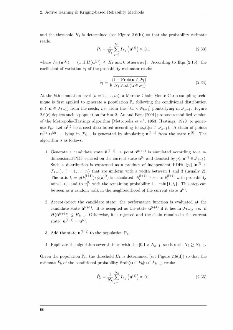
2. Active learning & Kriging-based Reliability Methods
and the threshold H1 is determined (see Figure 2.6(b)) so that the probability estimate
reads:
P1 =1
N1
N1∑
j=1
IF1
(
u(j))
≈ 0.1 (2.33)
where IF1(u(j)) = 1 if H(u(j)) ≤ H1 and 0 otherwise. According to Eqn.(2.15), the
coefficient of variation δ1 of the probability estimator reads:
δ1 =
√
1 − Prob(u ∈ F1)
N1 Prob(u ∈ F1)(2.34)
At the kth simulation level (k = 2, . . . , m), a Markov Chain Monte Carlo sampling tech-
nique is first applied to generate a population Pk following the conditional distribution
φn(.|u ∈ Fk−1) from the seeds, i.e. from the [0.1 × Nk−1] points lying in Fk−1. Figure
2.6(c) depicts such a population for k = 2. Au and Beck [2001] propose a modified version
of the Metropolis-Hastings algorithm [Metropolis et al., 1953; Hastings, 1970] to gener-
ate Pk. Let u(1) be a seed distributed according to φn(.|u ∈ Fk−1). A chain of points
u(1), u(2), . . . lying in Fk−1 is generated by simulating u(l+1) from the state u(l). The
algorithm is as follows:
1. Generate a candidate state u(l+1): a point v(l+1) is simulated according to a n-
dimensional PDF centred on the current state u(l) and denoted by p(.|u(l) ∈ Fk−1).
Such a distribution is expressed as a product of independent PDFs pi(.|u(l) ∈Fk−1), i = 1, . . . , n that are uniform with a width between 1 and 3 (usually 2).
The ratio ti = φ(v(l+1)i )/φ(u
(l)i ) is calculated. u
(l+1)i is set to v
(l+1)i with probability
min1, ti and to u(l)i with the remaining probability 1 − min1, ti. This step can
be seen as a random walk in the neighbourhood of the current state u(l).
2. Accept/reject the candidate state: the performance function is evaluated at the
candidate state u(l+1). It is accepted as the state u(l+1) if it lies in Fk−1, i.e. if
H(u(l+1)) ≤ Hk−1. Otherwise, it is rejected and the chain remains in the current
state: u(l+1) = u(l).
3. Add the state u(l+1) to the population Pk.
4. Replicate the algorithm several times with the [0.1 × Nk−1] seeds until Nk ≥ Nk−1.
Given the population Pk, the threshold Hk is determined (see Figure 2.6(d)) so that the
estimate Pk of the conditional probability Prob(u ∈ Fk|u ∈ Fk−1) reads:
Pk =1
Nk
Nk∑
j=1
IFk
(
u(j))
≈ 0.1 (2.35)
66

2.3. Sampling-based reliability methods
(a) Generation of a population P1 using φ2. (b) The performance function is evaluated ateach point of P1 and the threshold H1 is de-termined.
(c) The modified Metropolis-Hastings algorithmis employed to generate a population P2 followingthe conditional distribution φ2(.|u ∈ F1).
(d) The threshold H2 is determined.
(e) After 4 simulation levels, a population P5 isgenerated following the conditional distributionφ2(.|u ∈ F4).
(f) The threshold H5 is negative. It is then setto H5 = 0. P5 is calculated and the failure prob-ability is estimated by the product of the inter-mediate probabilities.
Figure 2.6: Subset Simulation procedure.
67

2. Active learning & Kriging-based Reliability Methods
The coefficient of variation δk of the probability estimator is:
δk =
√
1 − Prob(u ∈ Fk|u ∈ Fk−1)
Nk Prob(u ∈ Fk|u ∈ Fk−1)(1 + γk) (2.36)
where γk is a factor accounting for the correlation between the Nk points. The last level
is illustrated in Figure 2.6(e) and Figure 2.6(f). When the threshold Hk is negative, k is
set to m and Hm = 0. The failure probability estimate is finally obtained, on the basis of
Eqn.(2.32), by:
Pf =m∏
k=1
Pk (2.37)
The coefficient of variation δ of the failure probability estimator is given by:
δ =
√
√
√
√
m∑
k=1
δ2k (2.38)
Unlike Importance Sampling, Subset Simulation enables the detection of secondary
minima in other areas of space. Generality is thus preserved. Nevertheless, it inevitably
leads to a higher number of performance function evaluations. A slight modification of
Subset Simulation, known as iSubset, is proposed by Defaux et al. [2010] to reduce the
computational cost. Given that numerous simulation levels are unnecessary when an order
of magnitude of the failure probability is known, Conditional Sampling [Bernard and Fogli,
1987] is performed at the first simulation level. Such a sampling, depicted in Figure 2.7,
is characterized by an exclusion hyper-sphere centred on the origin of space with radius
βe to set.
Figure 2.7: First simulation level in iSubset.
68

2.4. Kriging-based reliability methods
2.3.5 Conclusion
In this section, various sampling-based reliability methods have been introduced to handle
problems involving small failure probabilities. Other alternatives such as Directional
Sampling [Ditlevsen et al., 1988] are acknowledged by the author but not considered in
the frame of this thesis.
2.4 Kriging-based reliability methods
Performance functions generally depend on responses of numerical models simulating the
mechanical behaviours of structures. Despite considerable advances in computer techno-
logy over the last two decades, a single evaluation of such models remains time-demanding
(several minutes to several hours) due to the continuous need for more faithful represent-
ations to the real mechanical behaviours. Numerous calls to performance functions are
consequently not possible in a short space of time. In addition, structures encountered in
industry are fortunately designed with codified rules leading to large safety margins, i.e.
small failure probabilities. The sampling-based reliability methods reviewed in the previ-
ous section are possible solutions to assess small probabilities, but they are inapplicable
with computationally demanding models, in so far as they still require a substantial num-
ber of performance function evaluations. This statement motivates the use of metamod-
elling as a means to conduct structural reliability analyses in a more practical amount of
time.
2.4.1 Principles of metamodelling
Metamodels are widespread in computational sciences and employed to predict the out-
come of a time-demanding function at any point, providing that the outcomes at a few
other points are known. These latter points are usually called the Design Of numerical
Experiments (DOE). Metamodels are attractive tools because they are fast to evaluate
in comparison with the actual functions. However, the selection of the DOE is of high
importance. The DOE must contain a sufficient number of points in order to ensure an
accurate approximation of the function, but it must also keep this number to a minimum
so as to remain affordable at a low cost. This latter condition is often referred to as the
parsimony constraint.
In structural reliability analysis, the metamodel H of the performance function H in
the standard space (or G for G in the physical space) is built to provide an approximate
failure domain F = u ∈ Un : H(u) ≤ 0. The integral formula of the failure probability
is then approximated by:
Pf ≈∫
Fφn(u)du1 . . . dun (2.39)
In practice, the failure probability is assessed by applying a sampling-based reliability
69

2. Active learning & Kriging-based Reliability Methods
method to the metamodel of the performance function. Note that a bias may be introduced
in the probability if the metamodel is not sufficiently refined.
Among metamodels, Quadratic Response Surfaces [Bucher and Bourgund, 1990; Das
and Zheng, 2000; Gayton et al., 2003] are the most popular although they are limited to
local interpolation. Polynomial Chaos [Ghanem and Spanos, 1991; Sudret and Der Ki-
ureghian, 2002] is an alternative to avoid this problem. However, the definitions of the
DOE and of the polynomial degrees are delicate issues [Blatman and Sudret, 2010]. More
recently, reliability methods based on Support Vector Machine have also been proposed
[Hurtado, 2004; Bourinet et al., 2011]. Finally, Kriging (also known as Gaussian process)
is investigated in this thesis for its stochastic and interpolation features (discussed in Sec-
tion 2.4.2.3). Its efficiency has been proven in structural reliability analysis [Romero et al.,
2004; Kaymaz, 2005; Bichon et al., 2008, 2009, 2011; Ranjan et al., 2008; Picheny et al.,
2010; Bect et al., 2011; Dubourg, 2011; Dubourg et al., 2011] and in related domains such
as uncertainty analysis and global sensitivity analysis [Kennedy et al., 2006; O’Hagan,
2006; Marrel et al., 2009].
2.4.2 Kriging theory
Kriging, pioneered by Krige [1951] and then theorized by Matheron [1973], considers the
performance function H as a realization of a Gaussian process H(u). The first step of
Kriging is the determination of the Gaussian process parameters according to the DOE.
Then, the best linear unbiased predictor is applied in order to estimate the outcome of
the performance function at an unobserved point. For more details on Kriging theory, the
reader may refer to Dubourg [2011, Chapter 1].
2.4.2.1 Identification of the Gaussian process
The model of the Gaussian process H(u) is expressed as [Sacks et al., 1989]:
H(u) = Y (u, η) + Z(u) (2.40)
where:
• Y (u, η) is the deterministic part giving an approximation of the response in mean.
It represents the trend of Kriging, and corresponds to a regression model that reads:
Y (u, η) = y(u)t η (2.41)
where y(u) = y1(u), . . . , yb(u)t is the vector of the basis functions and η =
η1, . . . , ηbt the vector of the regression coefficients. In this thesis, an ordinary
trend is favoured for Kriging, meaning that Y (u, η) is reduced to a scalar η. This
regression model is often sufficient, and other models do not necessarily bring any
70
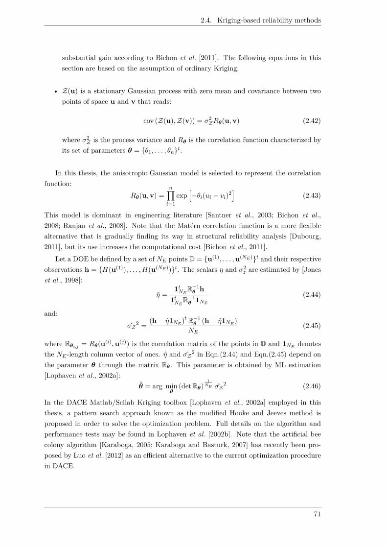
2.4. Kriging-based reliability methods
substantial gain according to Bichon et al. [2011]. The following equations in this
section are based on the assumption of ordinary Kriging.
• Z(u) is a stationary Gaussian process with zero mean and covariance between two
points of space u and v that reads:
cov (Z(u), Z(v)) = σ2ZRθ(u, v) (2.42)
where σ2Z is the process variance and Rθ is the correlation function characterized by
its set of parameters θ = θ1, . . . , θnt.
In this thesis, the anisotropic Gaussian model is selected to represent the correlation
function:
Rθ(u, v) =n∏
i=1
exp[
−θi(ui − vi)2]
(2.43)
This model is dominant in engineering literature [Santner et al., 2003; Bichon et al.,
2008; Ranjan et al., 2008]. Note that the Matérn correlation function is a more flexible
alternative that is gradually finding its way in structural reliability analysis [Dubourg,
2011], but its use increases the computational cost [Bichon et al., 2011].
Let a DOE be defined by a set of NE points D = u(1), . . . , u(NE)t and their respective
observations h = H(u(1)), . . . , H(u(NE))t. The scalars η and σ2z are estimated by [Jones
et al., 1998]:
η =1t
NER
−1θ h
1tNE
R−1θ 1NE
(2.44)
and:
σZ2 =
(h − η1NE)tR
−1θ (h − η1NE
)
NE(2.45)
where Rθi,j= Rθ(u(i), u(j)) is the correlation matrix of the points in D and 1NE
denotes
the NE-length column vector of ones. η and σZ2 in Eqn.(2.44) and Eqn.(2.45) depend on
the parameter θ through the matrix Rθ. This parameter is obtained by ML estimation
[Lophaven et al., 2002a]:
θ = arg minθ
(detRθ)1
NE σZ2 (2.46)
In the DACE Matlab/Scilab Kriging toolbox [Lophaven et al., 2002a] employed in this
thesis, a pattern search approach known as the modified Hooke and Jeeves method is
proposed in order to solve the optimization problem. Full details on the algorithm and
performance tests may be found in Lophaven et al. [2002b]. Note that the artificial bee
colony algorithm [Karaboga, 2005; Karaboga and Basturk, 2007] has recently been pro-
posed by Luo et al. [2012] as an efficient alternative to the current optimization procedure
in DACE.
71

2. Active learning & Kriging-based Reliability Methods
2.4.2.2 Kriging prediction
In the previous section, the parameters of the Gaussian process have been determined. The
next step is the prediction of the outcome H(u∗) at an unobserved point u∗. Beforehand,
let r(u∗) denote the correlation vector between u∗ and the points in D. Hence:
r(u∗) = Rθ(u∗, u(1)), . . . , Rθ(u∗, u(NE))t (2.47)
The Best Linear Unbiased Predictor (BLUP), denoted by H(u∗), is a Gaussian random
variable:
H(u∗) ∼ N(
µH(u∗), σ2H
(u∗))
(2.48)
with Kriging mean [Jones et al., 1998]:
µH(u∗) = η + r(u∗)tR
−1θ (h − η1NE
) (2.49)
and Kriging variance [Jones et al., 1998]:
σ2H
(u∗) = σZ2
1 − r(u∗)t
R−1θ r(u∗) +
(
1 − 1tNE
R−1θ r(u∗)
)2
1tNE
R−1θ 1NE
(2.50)
2.4.2.3 Noteworthy features
Kriging presents two intrinsic features that motivate its application to structural reliability
problems in this thesis:
• Interpolation: Figure 2.8(a) shows that the predictor interpolates the observations
h, i.e. ∀i, u(i) ∈ D, µH(u(i)) = H(u(i)). The proof of this begins by noting that,
for a point u(i) ∈ D, the correlation vector r(u(i)) is equivalent to the ith column of
Rθ. Hence, the correlation vector reads:
r(
u(i))
= Rθei (2.51)
where ei is the unit vector which is one for its ith row and zero for the others.
Eqn.(2.49) then becomes:
µH
(
u(i))
= η + eti (h − η1NE
) = etih = H
(
u(i))
(2.52)
Furthermore, Kriging variance is zero as Eqn.(2.50) changes to:
σ2H
(
u(i))
= σZ2
1 − r(u(i))tei +
(
1 − 1tNE
ei
)2
1tNE
R−1θ 1NE
= 0 (2.53)
72

2.4. Kriging-based reliability methods
• Measure of the prediction uncertainty: At a given point, Kriging not only
provides a prediction (Kriging mean) of the function outcome, but also a measure
of the prediction uncertainty (Kriging variance). As illustrated in Figure 2.8(b),
the Kriging variance may be used to find a point (or several) whose observation(s)
would lead to a substantial improvement in the metamodel’s accuracy. An iterative
enrichment of the DOE with wisely chosen points thus seems a relevant approach
to respect the parsimony constraint, i.e. to establish an accurate metamodel with a
limited number of function evaluations. Such an approach is commonly referred to
as an active learning method, and is further discussed in the next section.
(a) Kriging metamodel interpolating the obser-vations.
(b) Global prediction improved by evaluatingy = x sin(x) at the point having the largest Kri-ging variance, i.e. x = 10.
Figure 2.8: Illustrations of Kriging. The solid line is the function y = x sin(x). Thedashed line depicts the Kriging mean. The observations of the DOE are representedby the black dots. The light grey area corresponds to the 95% confidence interval, i.e.µH(x) ± 1.96 σH(x).
2.4.3 Active learning method
As far as the author is aware, Romero et al. [2004] are the first in applying Kriging to
structural reliability problems. In this early paper, the DOE of the Kriging metamodel
evolves following progressive lattice samplings, and consequently, does not consider the
additional information brought by the Kriging variance. The same statement can be
made regarding the method proposed by Kaymaz [2005]. Following these pioneering works,
Kriging is applied in an active learning scheme, where the DOE is iteratively enriched with
points selected through the evaluation of a learning function [Bichon et al., 2008; Ranjan
et al., 2008; Picheny et al., 2010; Bect et al., 2011; Dubourg, 2011; Echard et al., 2011a].
The general procedure of active learning can be summarized as follows:
1. Build the Kriging metamodel of H with an initial DOE.
73

2. Active learning & Kriging-based Reliability Methods
2. Find the point leading to the optimum of the learning function.
3. Enrich the DOE by evaluating H at such a point.
4. Build the new Kriging metamodel and go back to Step 2.
In structural reliability analysis, only points in the vicinity of the limit state H(u) = 0
represent relevant observations to refine the metamodel. Learning functions, discussed in
the following section, are specifically developed to find such points.
2.4.3.1 Learning function
Several learning functions are available in the literature related to structural reliability.
This section is restricted to the introduction of two functions that are easy to implement
and fast to evaluate.
Expected feasibility function
The active learning scheme of the Efficient Global Reliability Analysis (EGRA) [Bichon
et al., 2008] relies on the Expected Feasibility Function (EFF). Inspired by the contour
estimation work in Ranjan et al. [2008], EFF expresses the expectation that the actual
outcome of the performance function in a point u is expected to satisfy the equality
constraint H(u) = t [Bichon et al., 2011] (t = 0 for the limit state). The function reads:
EFF(u) = E[
ǫ(u) − min(|H(u) − t|, ǫ(u))]
(2.54)
where ǫ is set to focus the search in t ± ǫ. In Bichon et al. [2008], ǫ is proportional to the
Kriging standard deviation at each point: ǫ(u) = 2σH(u). By integrating over t ± ǫ, the
expectation becomes:
EFF(u) = µH(u)[
2Φ(
t−µH(u)σH(u)
)
− Φ(
t−ǫ(u)−µH(u)σH(u)
)
− Φ(
t+ǫ(u)−µH(u)σH(u)
)]
−σH(u)[
2φ(
t−µH(u)σH(u)
)
− φ(
t−ǫ(u)−µH(u)σH(u)
)
− φ(
t+ǫ(u)−µH(u)σH(u)
)]
+ǫ(u)[
Φ(
t+ǫ(u)−µH(u)σH(u)
)
− Φ(
t−ǫ(u)−µH(u)σH(u)
)]
(2.55)
High values of EFF are obtained for points having Kriging means close to the threshold
t, as well as points having large Kriging variances. The performance function is thus
evaluated at the location where EFF is maximized. The search of the optimum point is
further discussed in Section 2.4.3.2.
Learning function U
Inspired by Kushner’s criterion [1964] and the lower confidence bounding function [Cox
and John, 1997] in optimization, the learning function U [Echard et al., 2009] is proposed
74

2.4. Kriging-based reliability methods
to focus the search in the vicinity of the limit state. At an unobserved point u, it reads:
U (u) =|t − µH (u) |
σH (u)(2.56)
As depicted in Figure 2.9, U measures the distance in standard deviations between the
Kriging mean and the threshold t (set to 0 for the limit state). Since Gaussianity is
assumed by Eqn.(2.48), 1 − Φ(U(u)) for t = 0 represents the probability that H(u) has
an opposite sign (negative/positive) from µH(u). A small value of U(u) leads to a large
probability, and consequently, the performance function should be evaluated at the point
where U is minimized.
Figure 2.9: Illustration of the learning function U for three points u(1), u(2), u(3) withpositive Kriging means. The values of U are respectively 2, 1 and 0.8. The grey areas rep-resent the probabilities 1 − Φ(U(u(j))). The performance function H should be evaluatedat the point u(3).
Other alternatives
More sophisticated criteria such as the targeted Integrated Mean-Squared Error (tIMSE)
[Picheny et al., 2010] and the Stepwise Uncertainty Reduction (SUR) [Bect et al., 2011]
are available in the literature. Comparative studies of these learning functions have been
undertaken by Bect et al. [2011] and Li et al. [2011]. SUR is seen to converge the fastest to
a rough estimate of the failure probability, but its computational cost is larger than EFF
and U . In addition, the number of evaluations performed with U is rather comparable
to SUR’s when a refined estimate of the failure probability is targeted [Li et al., 2011].
Within this thesis, the learning function U thus seems acceptable for its simplicity and
efficiency.
75

2. Active learning & Kriging-based Reliability Methods
2.4.3.2 Search of the optimum
Learning functions are highly multimodal and consequently, finding the optimum is a
complex task. EGRA resorts to the gradient-free DIRECT (DIviding RECTangles) global
optimization algorithm [Jones et al., 1993; Gablonsky, 2001]. It consists of an iterative
division of the search domain into hyper-rectangles. The learning function EFF is cal-
culated at the hyper-centres, and the potentially optimal hyper-rectangles, determined
according to their size and EFF value, are sequentially divided. For further details on
the algorithm, the interested reader is referred to the DIRECT Matlab toolbox [Finkel,
2003]. In this thesis, the optimization is solved numerically by computing the learning
function at each point of a fixed population. Such a choice is seen as sufficient for the new
reliability methods devised in this research work (see Section 2.5).
2.4.4 Kriging prediction of the failure probability
In practice, the failure probability of Eqn.(2.39) is assessed by applying a sampling-based
reliability method to the refined metamodel of the performance function. For a given
population, Kriging offers two estimates of the failure probability:
• an estimate based on the mean values. The predicted failure domain is F = u ∈Un : µH(u) ≤ 0, and the Kriging mean indicator function IF (u) = 1 if µH(u) ≤0 and 0 otherwise is introduced to assess Pf .
• an estimate based on the full probabilistic information held in the Kriging predic-
tions [Picheny et al., 2010; Dubourg, 2011]. The predicted failure domain becomes
F = u ∈ Un : H(u) ≤ 0, and the probabilistic indicator function IF (u) =
Φ(U(u)) if µH(u) ≤ 0 and 1−Φ(U(u)) otherwise is introduced to assess Pf . Note
that U is not defined at the points of the DOE, but the sign of the performance func-
tion value is known in such points. Finally, Φ(U(u)) is 1 (respectively 0) when U(u)
tends to +∞ (respectively 0), thus both estimates converge to the same Pf .
In this thesis, the failure probability is estimated with the Kriging mean values. Hence
in the rest of the document, the predicted failure domain is defined as F = u ∈ Un :
µH(u) ≤ 0, and IF (u) refers to the Kriging mean indicator function. Note that the
second estimate is also calculated to observe the convergence in Section 2.5.3.
76

2.5. Active learning and Kriging-based Monte Carlo Simulation
2.5 Active learning and Kriging-based Monte Carlo Simu-
lation
2.5.1 Motivation
Kriging-based methods such as EGRA [Bichon et al., 2008] are mostly two-stage proced-
ures, where the construction of the Kriging metamodel through an active learning scheme
(stage 1) is completely independent from the subsequent sampling-based reliability analysis
(stage 2). Since stage 1 is performed regardless of the probability density, the performance
function may be observed in some areas that will not be covered by the random sampling
of stage 2. These observations consequently represent unnecessary evaluations that can
be avoided by merging both stages. In this thesis, a single-stage procedure is thus de-
vised to avoid these evaluations. The method is referred to as an Active learning and
Kriging-based Monte Carlo Simulation (AK-MCS) [Echard et al., 2009, 2010a,b, 2011a,b].
Following the classification concept [Hurtado, 2004], AK-MCS uses a Kriging metamodel
to classify a fixed Monte Carlo population into the safe and failure subsets, i.e. into the
points having positive performance function values and the points having negative per-
formance function values. The function U is evaluated at each point of the population,
and the Kriging metamodel is adaptively refined by evaluating the performance function
at the point leading to the smallest value of U(u). AK-MCS can be seen as a ‘guided’
Monte Carlo Simulation, where the sign of each point in the population is deduced from
a Kriging metamodel built with only a few wisely chosen observations of the performance
function.
2.5.2 Procedure
Let NE denote the number of performance function evaluations. Figure 2.10 depicts the
procedure which is as follows:
1. Generate a population PMCS according to φn†. It consists of the points u(j) =
u(j)1 , . . . , u
(j)n t, j = 1, . . . , NMCS to classify into the safe and failure subsets. These
points also represent candidates for future performance function evaluations.
2. Define the initial DOE. The performance function is evaluated at various points
in PMCS. In the original paper, around ten (NE ≈ 10) are uniformly drawn from
the population of candidates. However, such a selection may not lead to a sufficient
spread of the DOE due to the high density of candidates near the origin of space.
To convey a larger amount of information about the behaviour of the performance
function, space-filling designs such as Latin Hyper-cube Sampling [McKay et al.,
†For consistency of the document, the method is explained in the standard space but its application in
X n is also possible.
77

2. Active learning & Kriging-based Reliability Methods
1979] seem more suitable. Another alternative may, for instance, be a uniform
sampling of various points (e.g. 3) in each of the following subsets: u ∈ PMCS :
‖u‖ < 1, u ∈ PMCS : 2 ≤ ‖u‖ < 3, u ∈ PMCS : 3 ≤ ‖u‖ < 4... Note that
the number of observations is purposely small at first, since the DOE is iteratively
enriched in the subsequent active learning loop.
3. Perform the Kriging classification loop.
(a) Build the Kriging metamodel. An ordinary Kriging metamodel with an-
isotropic Gaussian correlation is built from the NE observations. DACE Mat-
lab/Scilab toolbox [Lophaven et al., 2002a] is used in this research work.
(b) Predict outcomes and assess Pf . The Kriging predictions of the points
in PMCS are computed: µH(u(j)), σH(u(j)), j = 1, . . . , NMCS. The Kriging
mean indicator function (see Section 2.4.4) is introduced in Eqn.(2.14) to es-
timate the failure probability Pf . The Kriging probabilistic indicator function
may also be used to provide a second estimate.
(c) Evaluate the learning function U and find u = arg minu∈PMCS
U(u). The
function U is evaluated at the [NMCS − NE ] unobserved points of PMCS. The
point u ∈ PMCS leading to the smallest value of U(u) is easily found.
(d) Test the stopping condition on learning. The condition reads: U(u) ≥ 2.
This arbitrary value refers to a 97.7% confidence level on the sign of the per-
formance function outcome. The author recommends deactivating the condition
in the early iterations, due to the fact that the procedure might wrongly stop
with an insufficient DOE. Experience has shown that the stopping condition
can be activated, once the DOE includes both safe and failure points.
(e) Enrich the DOE. If the stopping condition is not satisfied, the DOE is en-
riched by evaluating H(u). Hence NE = NE + 1, and the procedure goes back
to Step 3a to build the new Kriging metamodel.
4. End. If the stopping condition is met, each point of the population is considered
to be classified with a sufficient confidence level. Pf corresponds to the probability
estimated in Step 3b during the last loop. The coefficient of variation δ is calculated
using Eqn.(2.15). Note that if the coefficient of variation is too large, a new popu-
lation is generated, and the Kriging classification loop (Step 3) continues until the
stopping condition is satisfied again.
2.5.3 Validation
For the purpose of validating AK-MCS, examples which cover a wide variety of limit states
(high non-linearity, moderate number of random variables, non-convex and/or disconnec-
78

2.5. Active learning and Kriging-based Monte Carlo Simulation
Generate a population PMCS according to φn
u(j) = u(j)1 , . . . , u
(j)n t, j = 1, . . . , NMCS
Define the initial DOE: NE points ∈ PMCS
NE ≈ 10
Build the Kriging metamodel
Predict outcomes and
assess Pf using Eqn.(2.14)
Enrich the DOEwith (u, H(u))
Evaluate the learning function U
and find u = arg min
u∈PMCS
U(u)
Test the stopping condition on learning†:U(u) ≥ 2
NE = NE + 1
End
yes
no
†The stopping condition is activated, once the DOE includes both safe and failure points.
Figure 2.10: AK-MCS procedure. The light grey rectangle represents the Kriging classi-fication loop (Step 3).
ted domains of failure) are studied in this section. The reader may refer to Echard et al.
[2009, 2010a,b, 2011a,b] for further applications.
2.5.3.1 Two-dimensional series system with four branches
The first example is a series system with four branches, also studied by Waarts [2000];
Schueremans and Van Gemert [2005]. The performance function reads as follows:
H(U1, U2) = min
3 + (U1−U2)2
10 − (U1+U2)√2
;
3 + (U1−U2)2
10 + (U1+U2)√2
;
(U1 − U2) + 6√2;
(U2 − U1) + 6√2
(2.57)
where U1 and U2 are standard Gaussian distributed random variables. The problem is
represented in Figure 2.11. In this example, the population to classify into the safe and
failure subsets is composed of NMCS = 106 points. The initial DOE of AK-MCS is defined
79

2. Active learning & Kriging-based Reliability Methods
as ten points that are uniformly drawn from the population. The robustness of AK-MCS
is tested by applying the method to 100 different populations.
Figure 2.11: Safe (white) and failure (dark) domains on the example of the series systemwith four branches.
The number of performance function evaluations (NE) for the 100 AK-MCS runs is
represented in Figure 2.12. It ranges between 86 and 127, which is significantly less than
the number of points to classify (NMCS). In Table 2.1, the number of points misclassified
by AK-MCS in each of the 100 populations is reported. The classification is found to be
exact in 61 cases, meaning that the AK-MCS estimate of the failure probability is strictly
similar to the Monte Carlo estimate. Among the remaining 39 cases, the largest error, i.e.
3, is negligible in comparison with NMCS. In this example, AK-MCS with a median DOE
of 102 observations is shown to be equivalent to a Monte Carlo Simulation of 106 points
(see Table 2.2 for the median reliability results).
Figure 2.12: Number of performance function evaluations (NE) for 100 runs of AK-MCSon the example of the series system with four branches.
80

2.5. Active learning and Kriging-based Monte Carlo Simulation
Misclassified points Occurrence
0 61
1 27
2 7
3 5
Table 2.1: Number of misclassified points for 100 runs of AK-MCS on the example of theseries system with four branches.
Method NE Pf (×100) δ% (×100)
MCS 106 4.4591 × 10⁻³ 1.525
AK-MCS 102 4.4587 × 10⁻³ 1.527
Table 2.2: Median reliability results of Monte Carlo Simulation and AK-MCS over 100simulated populations on the example of the series system with four branches.
Figure 2.13(a) depicts an example of a population classified by AK-MCS. Figure 2.13(b)
gives the corresponding DOE. In accordance with the definition of the learning function,
the observations are mainly located in the close vicinity of the actual limit state. It
can also be seen that the accuracy of the predicted limit state, i.e. µH(u) = 0, is high
among the points of the population but decreases in areas such as the intersections of
the four branches that are not covered by the random sampling. These intersections
are low probability zones whose impact on the failure probability is negligible. Two-
stage procedures such as EGRA, which construct the Kriging metamodel regardless of
the probability density, would unnecessarily enrich the DOE with numerous points in the
vicinity of these discontinuities. Nevertheless, it is important to note that bounds can be
adjusted in EGRA in order to limit the domain of interest. For instance, [−5; 5] × [−5; 5]
would be sufficient to avoid the consideration of these intersections. Note also that EGRA
has recently been improved to deal with system reliability problems such as this example
[Bichon et al., 2011].
Figure 2.14(a) depicts the evolution of the two estimates of the failure probability,
i.e. the estimate based on the Kriging mean values and the estimate based on the full
probabilistic information held in the Kriging predictions (see Section 2.4.4). Both tend
towards a similar value after 70 evaluations. However, at this iteration, 72 points are
still incorrectly classified by AK-MCS. Figure 2.14(b) depicts the evolution of the learning
function’s minimum value. For this AK-MCS run, the stopping condition is met after
NE = 117 evaluations, and no misclassified points remain. As a conclusion, an extremely
accurate classification is guaranteed with the stopping condition U(u) ≥ 2, but the user
81

2. Active learning & Kriging-based Reliability Methods
may stop the procedure when the convergence of the two estimates is visually reached, as
long as a less refined result is acceptable.
(a) Classification by AK-MCS. The light greydots depict the points having a positive Krigingmean (safe), the black dots present a negativeKriging mean (failure).
(b) Final DOE of AK-MCS. The crosses are theinitial DOE, and the dots represent the pointsiteratively added to the DOE. The dark line de-picts the predicted limit state µH(u) = 0.
Figure 2.13: Illustration of AK-MCS on the example of the series system with fourbranches.
(a) Evolution of the failure probability estimates.The solid line is the estimate based on the Kri-ging mean values. The dashed line depicts theestimate based on the full probabilistic informa-tion held in the Kriging predictions.
(b) Evolution of the learning function’s min-imum value, i.e. U(u).
Figure 2.14: Evolutions of the failure probability estimates and learning function’s min-imum value on the example of the series system with four branches.
2.5.3.2 Modified Rastrigin function
The second example is based on the so-called Rastrigin function [Törn and Zilinskas, 1989].
This function is slightly modified to give a non-linear limit state involving non-convex and
82

2.5. Active learning and Kriging-based Monte Carlo Simulation
disconnected domains of failure (see Figure 2.15). The performance function reads:
H(U1, U2) = 10 −2∑
i=1
(
U2i − 5 cos (2π Ui)
)
(2.58)
where U1 and U2 are standard Gaussian variables. The population to classify into the safe
and failure subsets is composed of NMCS = 2.5 × 10⁴ points. The initial DOE of AK-MCS
is defined as ten points that are uniformly drawn from the population.
Figure 2.15: Safe (white) and failure (dark) domains on the example of the modifiedRastrigin function example.
The results are given in Table 2.3. 391 evaluations of the performance function are
sufficient to correctly classify the population into the safe and failure subsets (see Figure
2.16(a)). Figure 2.16(b) shows that the points of the DOE are located in the vicinity of
the different frontiers. In Figure 2.17(a), the failure probability estimate based on the
Kriging mean values is progressively improved. Such a behaviour can be related to the
gradual discovery of new failure zones. The two failure probability estimates are also seen
to tend towards a similar value after 360 evaluations of the performance function. At
this iteration, 40 points are still misclassified by AK-MCS. The evolution of the learning
function’s minimum value is given in Figure 2.17(b). As mentioned previously, the user
may stop the procedure when the convergence of the two estimates is visually reached, as
long as a less refined result is acceptable.
Method NE Pf δ%
MCS 2.5 × 10⁴ 7.43 × 10⁻² 2.23
AK-MCS 391 7.43 × 10⁻² 2.23
Table 2.3: Reliability results on the example of the modified Rastrigin function.
83

2. Active learning & Kriging-based Reliability Methods
(a) Classification by AK-MCS. The light greydots depict the points having a positive Krigingmean (safe), the black dots present a negativeKriging mean (failure).
(b) Final DOE of AK-MCS. The crosses are theinitial DOE and the dots represent the pointsiteratively added to the DOE. The dark line de-picts the predicted limit state µH(u) = 0.
Figure 2.16: Illustration of AK-MCS on the example of the modified Rastrigin function.
(a) Evolution of the failure probability estimates.The solid line is the estimate based on the Kri-ging mean values. The dashed line depicts theestimate based on the full probabilistic informa-tion held in the Kriging predictions.
(b) Evolution of the learning function’s min-imum value, i.e. U(u).
Figure 2.17: Evolutions of the failure probability estimates and learning function’s min-imum value on the example of the modified Rastrigin function.
2.5.3.3 Maximal deflection of a truss structure
The final example is a truss structure, proposed by Blatman and Sudret [2010], that is
illustrated in Figure 2.18. This application involves a moderate number of independent
random variables that are the Young moduli E1 and E2, the cross-section areas A1 and
A2, and the applied loads Pp for p = 1, . . . , 6. The characteristics of the random variables
are listed in Table 2.4. The response of the truss model is the deflection V1 at midspan.
84

2.5. Active learning and Kriging-based Monte Carlo Simulation
Given a threshold Vmax, the performance function reads:
G(E1, E2, A1, A2, Pp) = Vmax − V1 (2.59)
Three thresholds Vmax = 10; 11; 12 (cm) are considered so as to study the influence
of the probability level. One population is generated for each threshold. Their respective
sizes NMCS = 3.5 × 10⁴; 2 × 10⁵; 106 are determined to give an approximately 2.5%
coefficient of variation on the Monte Carlo estimator. The initial DOE of AK-MCS is
defined as ten points uniformly drawn from the population.
Figure 2.18: Truss structure with 23 members.
Variable Distribution Mean Std. dev.
E1, E2(Pa) Lognormal 2.1 × 10¹¹ 2.1 × 10¹⁰
A1(m2) Lognormal 2.0 × 10⁻³ 2.0 × 10⁻⁴
A2(m2) Lognormal 1.0 × 10⁻³ 1.0 × 10⁻⁴
P1 − P6(N) Gumbel 5.0 × 10⁴ 7.5 × 10³
Table 2.4: Random variables for the example of the truss structure.
The reliability results are reported in Table 2.5. For the three thresholds, no points
are misclassified by AK-MCS. Its failure probability estimates are then strictly similar to
Monte Carlo estimates. For a constant δ, the probability level is seen to have a limited
effect on the number of performance function evaluations as NE only varies between 110
and 128.
Figure 2.19(a) depicts, for the threshold Vmax = 10, the failure probability estimates
that are either based on the Kriging mean values or on the full probabilistic information
held in the Kriging predictions. In the previous examples, a large difference between them
is observed in the early iterations. For the truss structure, the estimates are extremely
similar, even before convergence. Stopping the procedure before observing this convergence
may lead to an inaccurate reliability result. To avoid this, the original stopping condition
depicted in Figure 2.19(b) should be preferred.
85

2. Active learning & Kriging-based Reliability Methods
Method Vmax NE Pf
10 3.5 × 10⁴ 4.33 × 10⁻²
MCS 11 2 × 10⁵ 8.38 × 10⁻³
12 106 1.53 × 10⁻³
10 110 4.33 × 10⁻²
AK-MCS 11 128 8.38 × 10⁻³
12 124 1.53 × 10⁻³
Table 2.5: Reliability results for δ ≈ 2.5% on the example of the truss structure.
(a) Evolution of the failure probability estimates.The solid line is the estimate based on the Kri-ging mean values. The dashed line depicts theestimate based on the full probabilistic informa-tion held in the Kriging predictions.
(b) Evolution of the learning function’s min-imum value, i.e. U(u).
Figure 2.19: Evolutions of the failure probability estimates and learning function’s min-imum value on the example of the truss structure for the threshold Vmax = 10.
2.5.4 Computational cost of the prediction step
In the previous part, AK-MCS is proven to be parsimonious with respect to the number
of performance function evaluations. The computational cost of the prediction step in
the AK-MCS procedure (Step 3b in Section 2.5.2) is now investigated so as to provide
recommendations on AK-MCS’ range of applications.
Consider the following n-dimensional problem proposed by Rackwitz [2001]:
G(X1, . . . , Xn) =(
n + 3σ√
n)−
n∑
i=1
Xi (2.60)
where Xi for i = 1, . . . , n are lognormal distributed random variables with mean value
µ = 1, and standard deviation σ = 0.2. The computational cost of the prediction step
86

2.5. Active learning and Kriging-based Monte Carlo Simulation
depends on the dimension of space (n), the size of the DOE at the current AK-MCS
iteration (NE), and the size of the population to predict (NMCS). A set of 18 situations
are simulated by combining the following values for the tuning parameters:
• dimension of space: n = 2; 10,
• size of the DOE at the current AK-MCS iteration: NE = 10; 100; 400,
• size of the population to predict: NMCS = 104; 105; 106.
The 18 simulations are conducted with a Intel Q9550 processor at 2.83 Ghz. Table 2.6
and Table 2.7 report the results in terms of the total CPU time, i.e. the sum of the CPU
time consumed by all of the CPUs utilized by the simulation. On the one hand, the CPU
time is obviously affected in a major way by the number of points in the population NMCS.
On the other hand, NE and n play relatively minor roles, at least in the studied ranges
of variation. According to these results, AK-MCS should be performed with a maximum
of 105 points to ensure a suitable computational cost. Failure probabilities higher than
10−3 can then be assessed with a reasonable coefficient of variation. Finally, note that the
parallel computing of the prediction step is also an easily-implementable solution in order
to reduce the time seen by the user.
NMCS
NE 10 100 400
104 < 1 1 4
105 2 8 38
106 13 82 370
Table 2.6: CPU time in seconds of the Kriging prediction for a dimension of space n = 2(e.g. for NMCS = 105 and NE = 100, the CPU time is 8 seconds). The simulations areconducted with a Intel Q9550 processor at 2.83 Ghz.
NMCS
NE 10 100 400
104 < 1 3 13
105 3 25 97
106 33 240 955
Table 2.7: CPU time in seconds of the Kriging prediction for a dimension of space n = 10(e.g. for NMCS = 105 and NE = 100, the CPU time is 25 seconds). The simulations areconducted with a Intel Q9550 processor at 2.83 Ghz.
87

2. Active learning & Kriging-based Reliability Methods
2.5.5 Conclusion
In this section, an Active learning and Kriging-based Monte Carlo Simulation (AK-MCS)
has been introduced. This ‘guided’ Monte Carlo Simulation is an iterative procedure
where a Kriging metamodel is used to classify a fixed population into the safe and failure
subsets. A learning function is devised to adaptively refine the metamodel. The validation
of the method on a set of examples shows that it provides an accurate classification of
the population while remaining parsimonious with respect to the number of performance
function evaluations (< 400 for the studied cases). In addition, its concept is similar
to crude Monte Carlo Simulations, making it an easily intelligible approach. Its imple-
mentation based on a Kriging toolbox such as DACE is also very accessible. Finally, it
is important to mention that AK-MCS has been successfully applied for the mechanical
and the thermo-chemical reliability assessments of an intensified heat exchanger reactor
[Boniface, 2010]. In Boniface’s PhD thesis, AK-MCS demonstrates the limits of FORM
and Quadratic Responses Surfaces.
2.6 Active learning and Kriging-based alternatives for small
probability cases
In spite of its parsimony regarding the number of performance function evaluations, AK-
MCS cannot be applied to applications involving small failure probabilities (at least not
in a short time). Three extensions of the original algorithm are thus proposed to handle
this case. With AK-MCS, they form the Active learning and Kriging-based Reliability
Methods, or AK-RM family [Gayton and Echard, 2012].
2.6.1 Active learning and Kriging based MCS under monotony
The first extension is proposed in the case of monotonic performance functions. The
Monte Carlo Simulation under monotony, exposed in Section 2.3.2, may be improved
considerably thanks to the Kriging classification loop of AK-MCS. The iterative selection
by the learning function U of new points in the vicinity of the limit state allows a drastic
reduction of the margin between the ensured safe and failure sub-domains. As a Kriging
prediction is necessary only for the few points lying in this margin, the computational
cost of the prediction step is substantially reduced. This extension is called AK-MCSm
(m standing for monotony).
2.6.1.1 Procedure
Let H be a monotonic performance function in the standard space. The ensured safe
and failure sub-domains are respectively denoted by E+ and E−. Figure 2.20 depicts the
procedure which is as follows:
88

2.6. Active learning and Kriging-based alternatives for small probability cases
1. Generate a population PMCS according to φn. The points are denoted by
u(j) = u(j)1 , . . . , u
(j)n t, j = 1, . . . , NMCS.
2. Perform crude MCSm until NE ≈ 10. MCS under monotony is run as explained
in Section 2.3.2. The number of points in PMCS and lying in the margin between E+
and E− is NR. N+ and N− refer to the number of points in the ensured safe and
failure sub-domains respectively.
3. Perform the Kriging classification loop.
(a) Build the Kriging metamodel. The metamodel is built from the NE ob-
servations. Note that the initial DOE consists of the ≈ 10 points evaluated by
crude MCSm at Step 2.
(b) Predict outcomes and assess Pf . The Kriging predictions of the NR points
lying in the margin are computed: µH(u(j)), σH(u(j)), j = 1, . . . , NR. The
estimate Pf of the failure probability reads:
Pf =N− +
∑NR
j=1 IF(
u(j))
NMCS(2.61)
where IF (u) is the Kriging mean indicator function.
(c) Evaluate the learning function U and find u. The function U is evaluated
at the remaining NR points. The point u leading to the smallest value of U(u)
is easily found.
(d) Test the stopping condition on learning. The condition reads: U(u) ≥ 2.
It is activated once the DOE includes both safe and failure points.
(e) Enrich the DOE. If the stopping condition is not satisfied, the DOE is en-
riched by evaluating H(u), and NE = NE + 1.
(f) Update NR, N+ and N−. Either E+ or E− is enlarged due to the new
observation H(u). The values of NR, N+ and N− are updated. The procedure
goes back to Step 3a to build the new Kriging metamodel.
4. End. If the stopping condition is met, each point of the population is considered
to be classified with a sufficient confidence level. Pf corresponds to the probability
estimated in Step 3b during the last loop. The coefficient of variation δ is calculated
using Eqn.(2.15). Note that if the coefficient of variation is too large, a new popula-
tion of points lying in the margin between E+ and E− is generated by means of an
accept/reject Monte Carlo sampling. The Kriging classification loop (Step 3) then
continues until the stopping condition is satisfied again.
89

2. Active learning & Kriging-based Reliability Methods
Generate a population PMCS according to φn
u(j) = u(j)1 , . . . , u
(j)n t, j = 1, . . . , NMCS
Perform crude MCSm until NE ≈ 10
NE ≈ 10; N+; N−; NR
Build the Kriging metamodel
Predict outcomes and
assess Pf using Eqn.(2.62)
Update NR,N+ and N−
Evaluate the learning function U
and find u = arg min
u
U(u)Enrich the DOEwith (u, H(u))
Test the stopping condition on learning†:U(u) ≥ 2
NE = NE + 1
End
yes
no
†The stopping condition is activated, once the DOE includes both safe and failure points.
Figure 2.20: AK-MCSm procedure. The light grey rectangle represents the Kriging clas-sification loop (Step 3).
2.6.1.2 Illustration
AK-MCSm is illustrated on an elementary R − S case:
G(R, S) = R − S (2.62)
where R and S are independent random variables. R is Gaussian with mean of 11 and
unit variance. S is uniform in the interval [6; 7.2]. The problem, depicted in Figure 2.21, is
considered in the standard space with the monotonic performance function H(UR, US). An
initial population of 106 points is generated according to φ2. Crude MCSm is performed
until NE = 10, and the Kriging classification loop is run until the stopping condition is
satisfied. Subsequently, 106 new points are simulated using φ2 and among them, only
those lying in the margin between E+ and E− are kept, so as to be also classified with
the Kriging loop. This procedure is repeated until the coefficient of variation of the failure
probability estimator is below ≤ 2.5%. To check its robustness, AK-MCSm is run for 100
different initial populations.
90

2.6. Active learning and Kriging-based alternatives for small probability cases
Figure 2.21: Safe (white) and failure (dark) domains of the elementary R − S case.
The median reliability results are reported in Table 2.8. For this application, AK-
MCSm with a median DOE of 24 observations is equivalent to a Monte Carlo Simulation
of 1.14 × 10⁸ points. Additionally, its computational cost is acceptable, since a median
CPU time of 106 seconds is measured. Note that AK-MCS is inapplicable, due to the
significant size of the population. Figure 2.22 shows the number of points misclassified
by AK-MCSm in each of the 100 populations. 84 cases present less than 4 misclassified
points, and the maximum value, i.e. 18, is negligible in comparison with the 1.14 × 10⁸
points. Figure 2.23 illustrates the final DOE for a given run of AK-MCSm. The Kriging
classification loop is seen to add points mainly in the vicinity of the limit state.
Method NE (×100) Pf (×100) CPU time in s (×100)
MCS 1.14 × 10⁸ 1.41 × 10⁻⁵ -
AK-MCSm 24 1.41 × 10⁻⁵ 106
Table 2.8: Median reliability results of Monte Carlo Simulation and AK-MCSm over 100simulated populations on the elementary R − S case. The targeted coefficient of variationis δ ≤ 2.5%. The median CPU time is given over 100 runs performed with a Intel Q9550processor at 2.83 Ghz.
2.6.1.3 Conclusion
AK-MCSm is a simple but efficient extension of AK-MCS for the case of monotonic per-
formance functions. It reduces the computational cost of the prediction step considerably,
and small failure probability cases can thus be handled in a short space of time.
91

2. Active learning & Kriging-based Reliability Methods
Figure 2.22: Number of misclassified points for 100 runs of AK-MCSm on the elementaryR − S case.
Figure 2.23: Final DOE of AK-MCSm on the elementary R − S case. The crosses depictthe 10 evaluations made with crude Monte Carlo Simulation under monotony at Step 2.The dots represent the 14 points added with the Kriging classification loop (Step 3). Thedark line depicts the predicted limit state.
2.6.2 Active learning and Kriging-based Importance Sampling
The application of the Kriging classification loop to a fixed population centred on the
MPFP is also an alternative to assess small failure probabilities. This approach represents
an improvement on the crude Importance Sampling technique with a Kriging metamodel.
It is referred to as AK-IS [Echard et al., 2011c, 2012]. By analogy with Importance
Sampling, AK-IS relies on the assumptions that the MPFP is well isolated and that no
secondary minima exist in other areas of space.
92

2.6. Active learning and Kriging-based alternatives for small probability cases
2.6.2.1 Procedure
Let H be the performance function in the standard space. Figure 2.24 depicts the AK-IS
procedure which is as follows:
1. ‘Roughly’ search the MPFP. The HLRF algorithm (or other) is performed in
order to find the MPFP P ⋆. The performance function H is evaluated at NE =
NFORM points. Note that a precise P ⋆ is not required. Performing a few iterations
of HLRF is sufficient to move sufficiently the centre of the population.
2. Generate a population PIS according to ϕn. It is recalled that the sampling
PDF ϕn is the n-dimensional Gaussian distribution centred on the approximated P ⋆
with uncorrelated components and unit variances. The points in the population PIS
are denoted by u(j) = u(j)1 , . . . , u
(j)n t, j = 1, . . . , NIS.
3. Perform the Kriging classification loop.
(a) Build the Kriging metamodel. The metamodel is built from the NE obser-
vations. Note that the initial DOE consists of the NFORM points evaluated at
Step 1. It may also be uniformly drawn from the population PIS as in AK-MCS.
(b) Predict outcomes and assess Pf . The Kriging predictions of the NIS points
are computed: µH(u(j)), σH(u(j)), j = 1, . . . , NIS. The estimate Pf of the
failure probability is assessed using Eqn.(2.29) with the Kriging mean indicator
function IF (u).
(c) Evaluate the learning function U and find u = arg minu∈PIS
U(u). The
function U is evaluated at the unobserved points of PIS. The point u ∈ PIS
leading to the smallest value of U(u) is easily found.
(d) Test the stopping condition on learning. The condition reads: U(u) ≥ 2.
It is activated once the DOE includes both safe and failure points.
(e) Enrich the DOE. If the stopping condition is not satisfied, the DOE is en-
riched by evaluating H(u). Hence NE = NE + 1, and the procedure goes back
to Step 3a to build the new Kriging metamodel.
4. End. If the stopping condition is met, each point of the population is considered
to be classified with a sufficient confidence level. Pf corresponds to the probability
estimated in Step 3b during the last loop. The coefficient of variation δ is calcu-
lated using Eqn.(2.31). Note that if the coefficient of variation is too large, a new
population is generated according to ϕn and the Kriging classification loop (Step 3)
continues until the stopping condition is satisfied again. At the end of the procedure,
the MPFP can be updated with the failure point which is the closest to the origin
of the standard space according to the Kriging predictions. The importance factors
are then calculated, as exposed in Section 2.3.3.2.
93

2. Active learning & Kriging-based Reliability Methods
‘Roughly’ search the MPFP P ⋆
NE = NFORM
Generate a population PIS according to ϕn
u(j) = u(j)1 , . . . , u
(j)n t, j = 1, . . . , NIS
Build the Kriging metamodel
Predict outcomes and
assess Pf using Eqn.(2.30)
Enrich the DOEwith (u, H(u))
Evaluate the learning function U
and find u = arg min
u∈PIS
U(u)
Test the stopping condition on learning†:U(u) ≥ 2
NE = NE + 1
End
yes
no
†The stopping condition is activated, once the DOE includes both safe and failure points.
Figure 2.24: AK-IS procedure. The light grey rectangle represents the Kriging classifica-tion loop (Step 3).
2.6.2.2 Two-dimensional non-linear performance function
AK-IS is first validated on a two-dimensional non-linear performance function H that
reads:
H(U1, U2) = 0.5(U1 − 2)2 − 1.5(U2 − 5)3 − 3 (2.63)
where U1 and U2 are standard Gaussian distributed random variables. The problem is
depicted in Figure 2.25. The HLRF algorithm is performed in order to find the single
MPFP. The number of HLRF iterations iFORM varies from 3 to 6 in order to observe the
effect of the precision of P ⋆ on the probability assessed by AK-IS. The corresponding P ⋆3
to P ⋆6 are illustrated in Figure 2.26. The population to classify into the safe and failure
subsets is composed of NIS = 104 points. The robustness of AK-IS is tested by applying
it to 4 sets of 100 different populations, one set for each iFORM value.
Table 2.9 reports the number of points misclassified by AK-IS. The maximum error is 3
which is negligible in comparison with NIS. Given the small number of misclassified points,
the AK-IS failure probability estimates are very similar to the corresponding Importance
94

2.6. Active learning and Kriging-based alternatives for small probability cases
Figure 2.25: Safe (white) and failure (dark) domains on the example of the two-dimensionalnon-linear performance function.
Figure 2.26: Locations of the MPFP P ⋆iFORM
on the example of the two-dimensional non-linear performance function.
Sampling estimates. The median reliability results are reported in Table 2.10. For the
different levels of iFORM, NE is seen to be significantly less than NIS. It is also observed, for
this example, that a less precise P ⋆ has a very slight impact on the number of evaluations
[NE−NFORM]. It thus seems suitable to limit the HLRF algorithm to a few iterations. Note
that the small increase in the coefficient of variation δ when the number of HLRF iterations
is reduced may be compensated by a larger population PIS. Finally, it is important to
mention that AK-IS is extremely fast, since the median CPU time of the AK-IS runs is
only 5 seconds with a Intel Q9550 processor at 2.83 Ghz.
95

2. Active learning & Kriging-based Reliability Methods
Misclassified pointsOccurrence
iFORM = 3 iFORM = 4 iFORM = 5 iFORM = 6
0 96 99 94 94
1 4 1 5 3
2 0 0 1 2
3 0 0 0 1
Table 2.9: Number of points misclassified by AK-IS on the example of the two-dimensionalnon-linear performance function. AK-IS is applied to 4 sets of 100 different populations,one set for each iFORM.
Method iFORM NE†(×100) Pf (×100) δ% (×100)
FORM 6 19 4.21 × 10⁻⁵ -
IS 6 19 + 104 2.86 × 10⁻⁵ 2.39
AK-IS 6 19 + 7 2.86 × 10⁻⁵ 2.39
AK-IS 5 16 + 7 2.86 × 10⁻⁵ 2.39
AK-IS 4 13 + 8 2.88 × 10⁻⁵ 2.48
AK-IS 3 10 + 8 2.87 × 10⁻⁵ 2.94†NE for IS and AK-IS is separated into the number required by FORM + the number for the Kriging
classification loop.
Table 2.10: Median reliability results over 100 runs of AK-IS for each iFORM on theexample of the two-dimensional non-linear performance function.
2.6.2.3 Dynamic response of a non-linear oscillator
The second example deals with a non-linear undamped single degree of freedom oscillator
that is depicted in Figure 2.27 [Rajashekhar and Ellingwood, 1993; Gayton et al., 2003;
Schueremans and Van Gemert, 2005]. The performance function reads:
G(C1, C2, M, R, T1, F1) = 3 R −∣
∣
∣
∣
∣
2 F1
M ω20
sin
(
ω20 T1
2
)∣
∣
∣
∣
∣
(2.64)
with ω0 =√
(C1 + C2) /M . The random variables are listed in Table 2.11. Note that the
distribution of the force F1 has changed in comparison to the previously cited research
papers in order to define a small failure probability, namely one that cannot be assessed
in a short space of time with AK-MCS. A reference failure probability estimate is set as
the median calculated over 100 runs of Monte Carlo Simulation with NMCS = 1.8 × 10⁸
points. AK-IS is applied to 100 populations, each composed of NIS = 104 points.
96
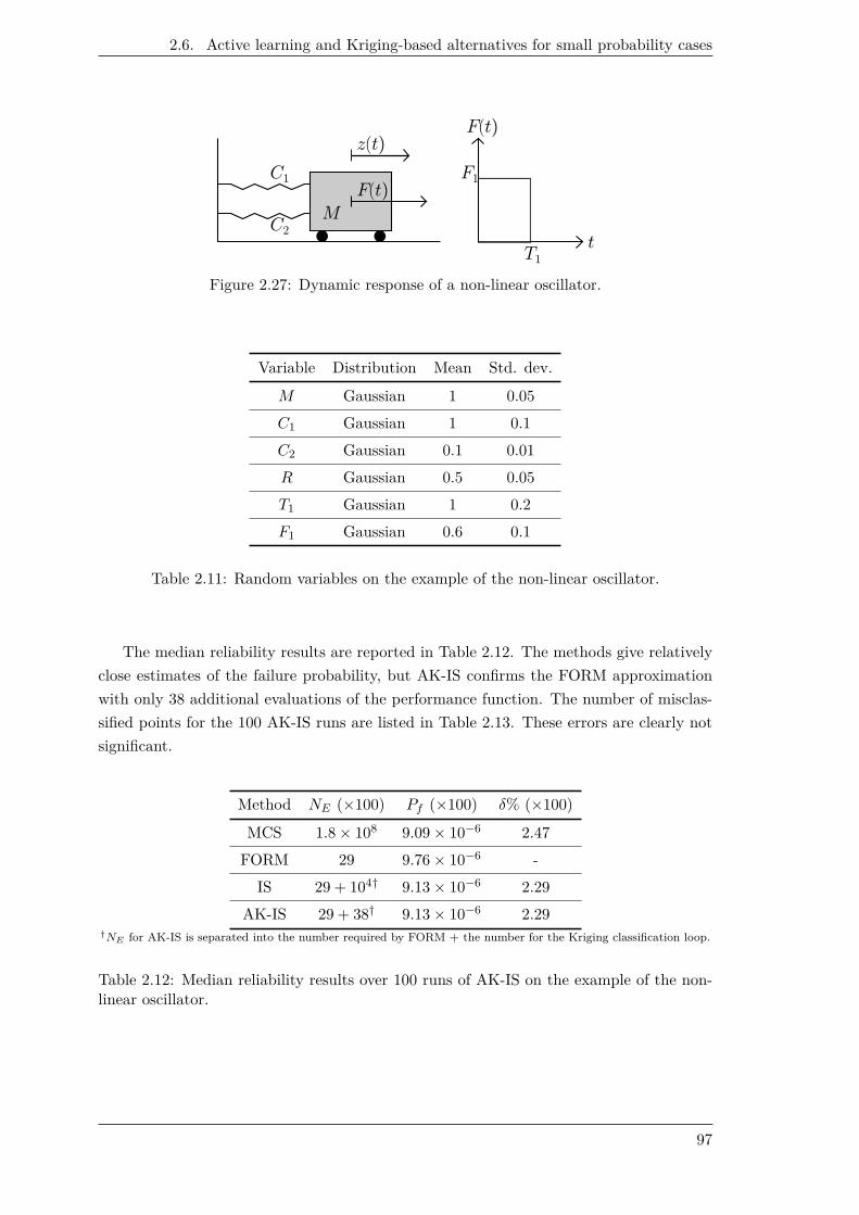
2.6. Active learning and Kriging-based alternatives for small probability cases
M
C1
C2
z(t)
F(t)
F(t)
t
F1
T1
Figure 2.27: Dynamic response of a non-linear oscillator.
Variable Distribution Mean Std. dev.
M Gaussian 1 0.05
C1 Gaussian 1 0.1
C2 Gaussian 0.1 0.01
R Gaussian 0.5 0.05
T1 Gaussian 1 0.2
F1 Gaussian 0.6 0.1
Table 2.11: Random variables on the example of the non-linear oscillator.
The median reliability results are reported in Table 2.12. The methods give relatively
close estimates of the failure probability, but AK-IS confirms the FORM approximation
with only 38 additional evaluations of the performance function. The number of misclas-
sified points for the 100 AK-IS runs are listed in Table 2.13. These errors are clearly not
significant.
Method NE (×100) Pf (×100) δ% (×100)
MCS 1.8 × 10⁸ 9.09 × 10⁻⁶ 2.47
FORM 29 9.76 × 10⁻⁶ -
IS 29 + 104† 9.13 × 10⁻⁶ 2.29
AK-IS 29 + 38† 9.13 × 10⁻⁶ 2.29†NE for AK-IS is separated into the number required by FORM + the number for the Kriging classification loop.
Table 2.12: Median reliability results over 100 runs of AK-IS on the example of the non-linear oscillator.
97

2. Active learning & Kriging-based Reliability Methods
Misclassified points Occurrence
0 97
1 3
Table 2.13: Number of misclassified points for 100 runs of AK-IS on the example of thenon-linear oscillator.
2.6.2.4 Conclusion
AK-IS is the extension of AK-MCS to a population centred on the MPFP. The number of
points to predict is considerably reduced in comparison with AK-MCS, and consequently,
small failure probabilities can be assessed in a very short space of time. Nevertheless, AK-
IS is limited to cases where the MPFP is well isolated, and where no secondary minima
exist in other areas of space.
2.6.3 Active learning and Kriging-based Subset Simulation
The last extension implements the Kriging classification loop within a Subset Simulation
(see Section 2.3.4) to reduce the computational cost of the two following steps:
• the evaluation of the performance function at the points in the first population P1.
• the evaluation of the performance function at the simulated candidate states in Step
2 of the modified Metropolis-Hastings algorithm.
In both cases, what matters is the position of the points in comparison with a given
threshold Hk (above or below) and not the performance function value. The Kriging
classification loop is appropriate to provide such information in a parsimonious way. This
extension is called AK-SS, and can be seen as an intermediary approach between the
general AK-MCS and the more specific AK-IS.
2.6.3.1 Procedure
Figure 2.28 depicts the AK-SS procedure. Let H be the performance function in the
standard space. Let a decreasing sequence of sub-domains F1 to Fm be, so that F1 ⊃F2 ⊃ . . . ⊃ Fm = F where Fk =
u ∈ Un : µH(u) ≤ µHk
.
First simulation level, k = 1
The first simulation level in Subset Simulation is a Monte Carlo Simulation. AK-MCS is
thus performed with some modifications to consider the threshold µH1. It goes as follows:
1. Generate a population P1 using φn. The points in P1 are denoted by u(j) =
u(j)1 , . . . , u
(j)n t, j = 1, . . . , N1.
98

2.6. Active learning and Kriging-based alternatives for small probability cases
Generate a population P1 according φn
u(j) = u(j)1 , . . . , u
(j)n t, j = 1, . . . , N1
Define the initial DOE: NE points ∈ P1
NE , k = 1
Determine the threshold µHk
Is µHk≤ 0?
Perform the Kriging classificationloop for µHk
until U(u) ≥ 2
k = m, µHm= 0 NE , k = k + 1
Perform the Kriging classificationloop for µHm
= 0 until U(u) ≥ 2
Generate a population of candidates
C(l+1) from the seeds
EndPerform the Kriging classificationloop for µHk−1
until U(u) ≥ 2
Accept/reject the candidate states:
C(l+1)
Add the states C(l+1) to Pk
Update NE Is Nk ≥ Nk−1?
yes
no
yes no
Figure 2.28: AK-SS procedure.
2. Define the initial DOE. The definition of the initial DOE is important as the
threshold µH1will be determined in Step 3 using a metamodel which has not yet
been adaptively refined. A relatively correct representation of the behaviour of the
performance function in the domain covered by P1 is thus beneficial at this early
stage. Latin Hyper-cube Sampling or the design proposed in Step 1 of AK-MCS
procedure (see Section 2.5.2) are possibilities.
3. Determine the threshold µH1.
(a) Build the Kriging metamodel. The metamodel is built from the NE obser-
vations.
99

2. Active learning & Kriging-based Reliability Methods
(b) Predict outcomes. The Kriging predictions of the N1 points are computed:
µH(u(j)), σH(u(j)), j = 1, . . . , N1.
(c) Determine µH1. The threshold µH1
characterizing the sub-domain F1 is de-
termined so that:
P1 =1
N1
N1∑
j=1
IF1
(
u(j))
≈ 0.1 (2.65)
where IF1(u) = 1 if µH(u) ≤ µH1
and 0 otherwise.
4. Is µH1≤ 0?. The threshold µH1
is set to 0 if found negative.
5. Perform the Kriging classification loop.
(a) Build the Kriging metamodel. The metamodel is built from the NE obser-
vations.
(b) Predict outcomes and assess P1. The Kriging predictions of the N1 points
are computed: µH(u(j)), σH(u(j)), j = 1, . . . , N1. The estimate P1 is then
improved using Eqn.(2.65).
(c) Evaluate the learning function U and find u = arg minu∈P1
U(u). To con-
sider the threshold µH1, the function U is modified as:
U (u) =|µH1
− µH (u) |σH (u)
(2.66)
It is evaluated at the [N1 − NE ] unobserved points of P1. The point u leading
to the smallest value of U(u) is easily found.
(d) Test the stopping condition on learning. The condition reads: U(u) ≥ 2.
It is activated once the DOE includes points on both sides of µH1.
(e) Enrich the DOE. If the stopping condition is not satisfied, the DOE is en-
riched by evaluating H(u). Hence NE = NE + 1, and the procedure goes back
to Step 5a to build the new Kriging metamodel.
6. If the stopping condition is met, each point of the population is considered to be
classified to the threshold µH1with a sufficient confidence level. P1 corresponds to
the probability estimated in Step 5b during the last loop. The coefficient of variation
δ1 is calculated using Eqn.(2.34). If µH1= 0, the procedure is finished. Otherwise,
the simulation level is set to k = k +1, i.e. k = 2, and a new population is generated
as explained in the next paragraph.
It is important to note that, following the principle of iSubset (see Section 2.3.4), the
population of the first simulation level may also be derived from Conditional Sampling.
100

2.6. Active learning and Kriging-based alternatives for small probability cases
Generation of the population for the kth simulation level, k = 2, . . . , mThe modified Metropolis-Hastings algorithm is applied to generate a population Pk fol-
lowing the conditional distribution φn(.|u ∈ Fk−1). It is recalled that in crude Subset
Simulation, the performance function is evaluated at each simulated candidate state to
know whether it lies in Fk−1 or not. The Kriging classification loop is applied to avoid
these evaluations. The procedure is as follows:
I. Generate a population of candidate states C(l+1) from the seeds. This is
similar to Step 1 of the modified Metropolis-Hastings algorithm, explained in Section
2.3.4. The population is composed of [P1 × Nk−1] candidate states (assuming that
this number is an integer).
II. Perform the Kriging classification loop.
(a) Build the Kriging metamodel. The metamodel is built from the NE obser-
vations.
(b) Predict outcomes. The Kriging predictions of the candidate states are com-
puted.
(c) Evaluate the learning function U and find u = arg minu∈C(l+1)
U(u). The
following function U is considered:
U (u) =|µHk−1
− µH (u) |σH (u)
(2.67)
The function is evaluated at each of the unobserved candidate states of C(l+1) in
order to determine whether they are classified with a sufficient confidence level.
The candidate state u leading to the smallest value of U(u) is easily found.
(d) Test the stopping condition on learning. The condition reads: U(u) ≥ 2.
(e) Enrich the DOE. If the stopping condition is not satisfied, the DOE is enriched
by evaluating H(u). Hence NE = NE +1, and the procedure goes back to Step
IIa to build the new Kriging metamodel.
III. Accept/reject the candidate states. If the stopping condition is met, each can-
didate state of C(l+1) is considered to be classified to the threshold µHk−1
with a
sufficient confidence level. The candidate states are accepted if they lie in Fk−1,
otherwise they are rejected, i.e. the Markov chains remain in the current state. The
population C(l+1) of the states is thus obtained.
IV. Add the states C(l+1) to Pk. The algorithm is then repeated with l = l + 1 until
Nk ≥ Nk−1.
101

2. Active learning & Kriging-based Reliability Methods
Calculation of Pk for simulation levels k = 2, . . . , mFor a simulation level k > 1, the procedure is slightly different from the first simulation
level. In Step 1, the population Pk is generated with the modified Metropolis-Hastings,
explained above. Step 2 is removed, as the DOE is composed of NE observations that
have already been made in the previous simulation levels. In Step 3c, the threshold µHk
characterizing the sub-domain Fk is determined so that Pk = 0.1. If found negative, µHk
is set to 0. In Step 5, the learning function U becomes:
U (u) =|µHk
− µH (u) |σH (u)
(2.68)
The last difference is the calculation of the coefficient of variation δk using Eqn.(2.36). The
procedure continues until µHk= µHm
= 0. The failure probability is then assessed using
Eqn.(2.37), and the coefficient of variation of the estimate is calculated with Eqn.(2.38).
2.6.3.2 Illustration
AK-SS is illustrated on the example of the parabolic limit state proposed by Der Kiur-
eghian and Dakessian [1998]. The performance function reads:
H(U1, U2) = a − U2 − b(U1 − c)2 (2.69)
where U1 and U2 are standard normal distributed random variables, a = 5, b = 0.2 and
c = 0. Note that the latter parameters differ slightly from the original paper. Parameters
a and b are set to define a small failure probability (≈ 10−5); one that cannot be assessed
in a short space of time with AK-MCS. Parameter c is set to give a symmetric limit
state (see Figure 2.29) and consequently two MPFPs. In such a case, AK-IS leads to a
biased failure probability estimate as only one MPFP is identified. AK-SS is proposed as
a more general approach that can deal with such reliability problems more precisely. A
reference failure probability estimate is defined as the median calculated over 100 runs of
Subset Simulation with an initial population of N1 = 105 points. AK-SS is conducted with
the same initial populations. The Kriging classification loop is also implemented within
iSubset. Its exclusion hyper-sphere presents a radius βe = 3.5.
The median reliability results are reported in Table 2.14. The median failure prob-
ability estimates of the three methods are extremely similar. However, the number of
performance function evaluations is reduced from 5 × 10⁵ to 38 for AK-SS and 27 for
AK-SS+iSubset. The iSubset trick also enables a decrease of the CPU time by 42% in
comparison with AK-SS. Figure 2.30(a) depicts the final DOE for a given run of AK-SS.
The Kriging classification loop is seen to add points mainly in the vicinity of the different
thresholds. The same comment can be made on the DOE of AK-SS+iSubset shown in
Figure 2.30(b).
102

2.6. Active learning and Kriging-based alternatives for small probability cases
Figure 2.29: Parabolic limit state with its symmetric MPFPs P ⋆1 and P ⋆
2 . The dark arearepresents the failure domain.
Method NE (×100) Pf (×100) δ% (×100) CPU time in s (×100)
SS 5 × 10⁵ 1.91 × 10⁻⁵ 3.42 -
AK-SS 38 1.90 × 10⁻⁵ 3.28 260
AK-SS+iSubset† 27 1.92 × 10⁻⁵ 3.27 150†The radius of the hyper-sphere is βe = 3.5.
Table 2.14: Median reliability results over 100 runs of AK-SS and AK-SS+iSubset onthe example of the parabolic limit state. The median CPU time is given for 100 runsperformed with a Intel Q9550 processor at 2.83 Ghz.
(a) Final DOE of an AK-SS run. Five simulationlevels are observed.
(b) Final DOE of an AK-SS+iSubset run.Three simulation levels are observed (the secondone is extremely close to the limit state).
Figure 2.30: Illustration of AK-SS and AK-SS+iSubset on the example of the paraboliclimit state. The crosses depict the initial DOE. The dots represent the points iterativelyadded to the DOE with the Kriging classification loop. The solid line is the limit state.The dashed lines are the different thresholds H(u) = µHk
.
103

2. Active learning & Kriging-based Reliability Methods
2.6.3.3 Conclusion
AK-SS corresponds to the implementation of the Kriging classification loop within Subset
Simulation. Unlike AK-IS, AK-SS is not based on any assumption of the limit state’s
shape. Nevertheless, it requires more predictions and performance function evaluations.
The computational cost of AK-SS may be improved by performing the first simulation level
with Conditional Sampling, as in iSubset. Finally, AK-SS can be seen as an intermediary
approach between the general AK-MCS and the more specific AK-IS.
2.7 Conclusion
A family of Kriging-based reliability methods called AK-RM has been presented in this
chapter. These methods represent improvements on various classical sampling techniques
through the addition of an iterative Kriging classification loop. The basic idea is to use the
predictions of the Kriging metamodel in order to classify a fixed population into its safe
and failure subsets, using the least possible number of performance function evaluations. A
specific learning function identifies the evaluations that should be carried out to adaptively
refine the metamodel in the vicinity of the limit state. To a certain extent, the AK-RM
family can be seen as ‘guided’ sampling techniques. Their validations on a set of examples
show that they are accurate classifiers, while remaining parsimonious with respect to the
number of performance function evaluations.
The first method of the AK-RM family (see Figure 2.31) is AK-MCS, which corres-
ponds to the combination of the Kriging classification loop with Monte Carlo Simulation.
Although it is the most general approach, it becomes computationally demanding for fail-
ure probabilities below 10−3. Alternatives are thus introduced to consider such reliability
levels. Given that the performance function of many structures happens to be monotonic
with respect to its random variables, AK-MCSm is suggested to take advantage of this
monotony. AK-IS is another approach that classifies points simulated in the vicinity of
the MPFP. The computational cost is considerably reduced, but the approach relies on
the hypothesis that the weight of the failure probability is well located. Finally, AK-SS
based on Subset Simulation is proposed as an intermediary method between the general
AK-MCS and the more specific AK-IS.
Note that the adaption of the Kriging classification loop to the case of multiple failure
modes (or system reliability) is currently being studied. It is also important to mention
that the principles of AK-RM have recently been applied to the tolerance Inspection of
Large Surfaces (AK-ILS) [Dumas et al., 2012, 2013]. Inspired by the learning function U ,
AK-ILS iteratively identifies the points that should be measured in order to determine
with the least number of measurements the conformity (or non-conformity) of the surface
being inspected.
104

2.7. Conclusion
AK-MCS
general but limited
to Pf ≥ 10−3
AK-MCSm
for monotonic
performance functions
Reliability analysis
AK-RM
AK-IS
for well isolated
MPFP
AK-SS
trade-off between
AK-MCS and AK-IS
AK-System
for system reliability
problems
Tolerance inspection
AK-ILS
Figure 2.31: AK-RM family and current extensions.
105
2. Active learning & Kriging-based Reliability Methods
In industry, structures are designed with large safety margins, so that
failure has a small probability of occurring. Furthermore, performance
functions characterizing structural failure scenarios often depend on re-
sponses of numerical models whose evaluations are time-demanding. As
a consequence, the classical sampling-based reliability methods such as
Monte Carlo Simulation cannot be applied. Following this statement,
metamodelling is proposed in this chapter as a means to conduct struc-
tural reliability analyses in a more practical amount of time. Metamod-
els are fast-to-evaluate approximations of the performance function.
They require a Design Of numerical Experiments (DOE), i.e. a set of
points where the values of the computationally demanding performance
function are known. The selection of the DOE is of high importance,
as it must contain a sufficient number of points to build an accurate
metamodel, but must also keep this number to a minimum so as to re-
main practical in a short space of time. In this chapter, the Kriging
metamodel is selected because it presents two crucial features. First,
it interpolates the points in the DOE. Second, it provides a measure of
the prediction uncertainty (the Kriging variance). The latter feature
enables the use of Kriging in an active learning scheme which is an it-
erative enrichment of the DOE with well selected points. Within the
frame of structural reliability analysis, the best points to select are loc-
ated in the vicinity of the limit state. A learning function named U and
based on the Kriging variance is specifically proposed in this chapter to
identify these points. Finally, this learning function is employed within
four Active learning and Kriging-based Reliability Methods (AK-RM)
to deal with problems involving computationally demanding models and
small failure probabilities. The validation of these methods on a set of
examples shows that they provide accurate failure probability estimates
while remaining parsimonious with respect to the number of perform-
ance function evaluations.
Chapter summary
106

3 Application to the case studies of
the APPRoFi project
Contents
3.1 Introduction . . . . . . . . . . . . . . . . . . . . . . . . . . . . . . . . 108
3.2 Bolted joint in an aircraft engine . . . . . . . . . . . . . . . . . . . . 108
3.2.1 Fatigue behaviour . . . . . . . . . . . . . . . . . . . . . . . . . . . . . 108
3.2.2 Load modelling . . . . . . . . . . . . . . . . . . . . . . . . . . . . . . . 111
3.2.3 Numerical model . . . . . . . . . . . . . . . . . . . . . . . . . . . . . . 113
3.2.4 Reliability assessment . . . . . . . . . . . . . . . . . . . . . . . . . . . 114
3.2.5 Results . . . . . . . . . . . . . . . . . . . . . . . . . . . . . . . . . . . 115
3.3 Blade support case study . . . . . . . . . . . . . . . . . . . . . . . . . 115
3.3.1 Fatigue behaviour . . . . . . . . . . . . . . . . . . . . . . . . . . . . . 116
3.3.2 Material properties . . . . . . . . . . . . . . . . . . . . . . . . . . . . . 118
3.3.3 Load modelling . . . . . . . . . . . . . . . . . . . . . . . . . . . . . . . 119
3.3.4 Numerical model . . . . . . . . . . . . . . . . . . . . . . . . . . . . . . 123
3.3.5 Reliability assessment . . . . . . . . . . . . . . . . . . . . . . . . . . . 124
3.3.6 Results . . . . . . . . . . . . . . . . . . . . . . . . . . . . . . . . . . . 125
3.4 Conclusion . . . . . . . . . . . . . . . . . . . . . . . . . . . . . . . . . 126
107

3. Application to the case studies of the APPRoFi project
3.1 Introduction
This chapter is devoted to the application of the probabilistic approach exposed in Chapter
1 to two case studies submitted by SNECMA within the frame of the APPRoFi project.
These case studies involve computationally demanding numerical model and small failure
probabilities. To enable a prompt reliability assessment, the global methodology developed
in the APPRoFi project is applied. The probabilistic approach explained in Chapter
1 forms the backbone of this methodology. The computational cost of the structural
reliability analysis is then reduced in two ways. First, the CPU time of the numerical model
evaluation is optimized by LMT-ENS Cachan. The LATIN method [Ladevèze, 1999] is
used in order to diminish the time spent for a single model evaluation. A multiparametric
strategy [Boucard and Champaney, 2003] is also applied in order to decrease the time
demand of succeeding computations. For further details on these two numerical methods,
the reader may refer to Relun [2011] whose thesis also contributes to the APPRoFi project.
Second, Kriging-based reliability methods presented in Chapter 2 are applied to determine
the failure probability and the influent parameters on structural reliability with a limited
number of numerical model evaluations.
Note that, for confidentiality reasons, axis graduations are not displayed
and no order of magnitude of the failure probability is mentioned.
3.2 Bolted joint in an aircraft engine
The first case study is proposed by SNECMA’s aviation branch. It deals with a bolted
joint of blisks (also known as bladed disks and integrally bladed rotors) located in a jet
engine. One of these blisks undergoes high stresses in the vicinity of an oil evacuation hole.
The aim of the study is to determine the probability of crack initiation at this geometric
discontinuity due to fatigue loads. Figure 3.1 depicts the flowchart of the probabilistic
approach for this case study. The different steps of this flowchart are discussed below.
3.2.1 Fatigue behaviour
Probabilistic S −N curves are implemented in this thesis to model the dispersion observed
in a data set of 361 purely tensile (R = 0) fatigue tests provided by SNECMA. The
deterministic model of the S − N curves is selected as a ‘double’ Basquin’s relation, where
the change of slope is set to an arbitrary number of cycles NC . The deterministic model
is expressed as the median range ∆σ50%:
∆σ50% =
Bi N bi for N ≤ NC
Bs N bs for N > NC
(3.1)
108

3.2. Bolted joint in an aircraft engine
deterministic material
prop. and geometry
xm, xg
random load
param. µT (ω), σT (ω)random isoprob. S −N
curve Uf for R = 0
xm, xg µT , σT uf
sequence of Neq
rotational speed cycles
numerical model
analytical expression
EF cycle with R = 0Ωeq,max(µT , σT , bi, bs, Neq)
max. principal stress for R = 0∆σ1(xm,xg, µT , σT , bi, bs, Neq)
strength value
∆r(uf , Neq)
G = ∆r −∆σ1
AK-RM
failure probability and
importance factors
bi, bs
Figure 3.1: Probabilistic approach for the bolted joint case study.
109

3. Application to the case studies of the APPRoFi project
The parameters of the three probabilistic S − N curve models discussed in Section 1.3.5
are inferred according to the data set. ESOPE, ESOPE 2 and Guédé’s model are depicted
in Figure 3.2. Relatively different behaviours are observed for these three S − N curve
models. The impact of modelling on the strength value for three numbers of cycles to
failure N1, N2 and N3 is quantified in Table 3.1. The median curves are seen to be rather
similar (particularly ESOPE 2 and Guédé’s model), but the isoprobability curves at 2.5%
and 97.5% present significant differences. Model selection is done using AIC, BIC and
the p-values of Kolmogorov-Smirnov tests. Table 3.2 reports the values of these criteria.
ESOPE 2 is selected in the frame of this study, due to the fact that it presents the smallest
AIC and BIC values and that there is not enough evidence to reject its initial hypothesis
at a sensible level (5%). As mentioned in Section 1.3.5, all the isoprobability S −N curves
of ESOPE 2 feature the same Basquin’s slopes bi and bs, i.e. bi(Uf ) = bi, and bs(Uf ) = bs
(Uf is recalled to denote the random isoprobability S − N curve).
(a) ESOPE. (b) ESOPE 2.
(c) Guédé’s model.
Figure 3.2: Fitting of ESOPE, ESOPE 2 and Guédé’s models to the fatigue tests for thebolted joint case study. The solid line represents the median trend. The dashed lines arethe isoprobability S − N curves defined at 2.5% and 97.5%.
110

3.2. Bolted joint in an aircraft engine
ModelN1 N2 = NC N3
2.5% 50% 97.5% 2.5% 50% 97.5% 2.5% 50% 97.5%
ESOPE 1.00 1.00 1.00 1.00 1.00 1.00 1.00 1.00 1.00
ESOPE 2 0.96 1.01 1.05 0.98 0.97 0.96 1.06 1.00 0.95
Guédé 0.87 1.01 1.12 1.03 0.97 1.08 1.08 1.00 0.93
Table 3.1: Impact of the S −N curve model on the strength value for the bolted joint casestudy. The results for different lives N1, N2 and N3 (see Figure 3.2) are normalized tothe strength value found using ESOPE. The percentages (2.5%, 50%, 97.5%) refer to theisoprobability curves.
Model AIC BIC p-value
ESOPE 9103 9119 5 × 10⁻⁴
ESOPE 2 8980 8996 0.09
Guédé 9011 9027 0.13
Table 3.2: Measures of the relative goodness of fit of the probabilistic S − N curve modelsfor the bolted joint case study.
3.2.2 Load modelling
The bolted joint of blisks is subjected to various loadings including preloads and centri-
fugal, radial and axial loads of the blades. Deterministic sensitivity studies conducted by
LMT-ENS Cachan prove that the centrifugal load is the main source of fatigue damage
and that the variations of the other loads have no significant impact on the structural
response. The latter loads are thus set as deterministic, and only the uncertainty of the
centrifugal load is considered in this study.
The centrifugal load is derived from the rotational speed Ω which is associated with
the thrust that must be generated in order to make the aircraft move. Given that the
greatest thrust is observed at takeoff, the fatigue load is defined as a sequence of Neq
cycles (0, Ωi,max) where Neq is the number of flights performed by the engine during its
design life and Ωi,max the maximum rotational speed observed at the ith takeoff (see Fig-
ure 3.3). The load sequence presents variable ranges which are in fact due to the climatic
fluctuations of temperature at takeoff†. In this study, the load sequence is assumed to be
a mix of five missions A, B, C, D, E characterized by maximum rotational speeds Ω =
ΩAmax, ΩB
max, ΩCmax, ΩD
max, ΩEmaxt at takeoff and temperatures T = T A, T B, T C, T D, T Et.
†The thrust generated by the jet engine is inversely proportional with ambient temperature. The
rotational speed required for reaching takeoff thrust is then linked to temperature in the following way:
the higher temperature, the higher the rotational speed.
111

3. Application to the case studies of the APPRoFi project
Table 3.3 reports the characteristics of these missions. To consider the uncertainties of
the centrifugal load, the percentages of occurrence pA, pB, pC, pD, pE of the missions are
random variables. No load data are provided to determine the scatter of these percent-
ages, but according to SNECMA flight experts, an aircraft mostly takes off from a given
base and is consequently subjected to rather similar temperatures at takeoff through-
out its design life. Following this statement, the bolted joint of blisks is exposed to a
dominant mission (or rotational speed), and secondary missions are less and less fre-
quent as their corresponding temperatures at takeoff are further from the temperature
of the dominant mission. For a given aircraft, the temperature at takeoff can be mod-
elled by a squared exponential function. This function is considered as being a Gaussian
PDF fT (t) (see Figure 3.4). Given a mean µT and a standard deviation σT , the values
fT (T A), fT (T B), fT (T C), fT (T D), fT (T E) of the Gaussian PDF can be calculated, and
each percentage of occurrence pm for m = A, . . . , E can be defined as:
pm =fT (T m)
∑Ei=A fT (T i)
(3.2)
Following Eqn.(3.2), the percentages are fully characterized by the PDF’s parameters µT
and σT . Setting these parameters as random variables thus enables random percentages
to be defined. In agreement with SNECMA engineers, the mean µT (ω) is considered as
a uniform random variable on the interval [min (T) − 5; max (T) + 5], and the standard
deviation σT (ω) as a Gaussian variable of mean 16 and variance 4.
Figure 3.3: Sequence of cycles in maximum rotational speed Ω at takeoff.
By drawing a realization µT, σT , a sequence of Neq rotational speed cycles is gen-
erated. This sequence is composed of Neq × pm(µT, σT ) cycles (0, Ωmmax) for each m =
A, . . . , E. Using the deterministic Basquin’s slopes bi and bs, the virtual sequence is trans-
formed into an EF cycle (0, Ωeq,max(µT, σT , bi, bs, Neq)) repeated Neq times.
112

3.2. Bolted joint in an aircraft engine
Mission A B C D E
Ωmax 1.028 1.012 1.000 0.990 0.975
T 33.1 14.4 0 -11.2 -28.7
Table 3.3: Missions characterized by their maximum rotational speeds Ωmax and temper-atures T at takeoff. The rotational speeds are normalized to ΩC
max. The temperature isgiven as the difference with T C.
Figure 3.4: Gaussian distribution of the temperature at takeoff for a given aircraft. Thedistribution is characterized by a mean µT and a standard deviation σT . The valuesfT (T A), fT (T B), fT (T C), fT (T D), fT (T E) are used to define the percentages of occur-rence following Eqn.(3.2).
3.2.3 Numerical model
In a preliminary sensitivity analysis by LMT-ENS Cachan, the material properties and
geometry of the numerical model are proven to have no significant impact on the struc-
tural response, thus they are considered as deterministic parameters respectively denoted
by xm, xg. The EF cycle (0, Ωeq,max(µT, σT , bi, bs, Neq)) is applied to the numerical
model. The output of interest is the cycle of the maximum principal stress (σI,min, σI,max)
interpreted as a cycle being undergone Neq times by the bolted joint of blisks. This
cycle features a maximum value σI,max(xm, xg, µT , σT , bi, bs, Neq) which is reached when
Ωeq,max(µT, σT , bi, bs, Neq) is applied, and a minimum value σI,min(xm, xg) for a rotational
speed of zero. Given that deterministic preloads are also applied to the numerical model,
σI,min(xm, xg) differs from 0 when the engine is not in operation. Therefore, the stress
cycle is not purely tensile (R ≈ −0.05), and a mean correction is necessary to enable
fatigue calculation. To convert the stress cycle into its purely tensile equivalent, a model
of the Haigh diagram is to be assumed and the tensile strength of the material must be
known. In agreement with SNECMA engineers, the mean correction is not performed.
113

3. Application to the case studies of the APPRoFi project
Hence, σI,min(xm, xg) is said to be 0, and the range ∆σI(xm, xg, µT , σT , bi, bs, Neq) thus
corresponds to σI,max(xm, xg, µT , σT , bi, bs, Neq).
Numerical model evaluations by LMT-ENS Cachan show that a linear relation can be
assumed between σI,max(xm, xg, µT , σT , bi, bs, Neq) (≡ ∆σI(xm, xg, µT , σT , bi, bs, Neq)) and
Ωeq,max(µT , σT , bi, bs, Neq) in the interval [ΩEmax; ΩA
max] (see Figure 3.5). Given that the
geometry and the material properties are deterministic, the relation remains the same for
any realization of the random variables. The numerical model is therefore replaced with
an analytical expression whose computational cost is free.
Figure 3.5: Numerical model evaluations (white dots) by LMT-ENS Cachan showing thata linear relation exist between σI,max and Ωeq,max in the interval [ΩE
max; ΩAmax] (black dots).
3.2.4 Reliability assessment
Table 3.4 recapitulates the random variables of the reliability problem. The performance
function G compares the range ∆σI(xm, xg, µT , σT , bi, bs, Neq) with the drawn strength
range ∆r(uf , Neq) at Neq cycles. AK-IS and AK-SS are implemented to pilot structural
reliability analyses. Given that the model is replaced with an analytical expression, Im-
portance Sampling and Subset Simulation are also applied to confirm results.
Random variable Denomination Distribution Parameters
µT (ω) Mean of fT (T ) Uniform [min (T) − 5; max (T) + 5]
σT (ω) Std. dev. of fT (T ) Gaussian µσT= 16; σσT
= 2
Uf Isoprob. S − N curve Gaussian µUf= 0; σUf
= 1
Table 3.4: Random variables of the bolted joint case study.
114

3.3. Blade support case study
3.2.5 Results
The reliability results are reported in Table 3.5. A population of 1.2 × 10⁴ points centred
on the approximated MPFP is classified using AK-IS and Importance Sampling. Similar
probabilities are obtained, but AK-IS requires only 54 evaluations of the performance
function. AK-SS and SS are performed to verify whether the MPFP is well isolated. For
computational reasons, AK-SS is performed with an initial population of 2 × 10⁴ points,
whereas SS is performed with a significantly larger initial population. The results prove
that the MPFP is indeed isolated.
Method NE P normf δ
FORM 9 1.00 -
IS 1.2 × 10⁴ 0.66 2.41%
SS 3.5 × 10⁶ 0.65 2.10%
AK-IS 54 0.66 2.41%
AK-SS 451 0.66 10.56%
Table 3.5: Reliability results for the case study of the bolted joint. The failure probabilitiesare normalized to the FORM approximation.
The elasticities of the Hasofer-Lind reliability index with respect to the standard de-
viations of µT (ω), σT (ω) and Uf are reported in Table 3.6. For this case study, the S − N
curve model is the most influent parameter on structural reliability.
Load Fatigue
EσµTEσσT
EσUf
−3.4 × 10⁻² −3.7 × 10⁻⁴ −0.973
Table 3.6: Elasticities of the Hasofer-Lind reliability index with respect to the standarddeviations of µT (ω), σT (ω) and Uf for the case study of the bolted joint.
3.3 Blade support case study
The blade support case study (see Figure 3.6) is an aerospace application which has already
been considered in the DEFFI project [Bignonnet and Lieurade, 2007; Bignonnet et al.,
2009; Ferlin et al., 2009; Lefebvre et al., 2009]. During its design life, the blade support is
shear-loaded by random fatigue displacements in its transverse direction. The aim of the
study is to determine the probability of crack initiation due to these fatigue loads. Figure
115

3. Application to the case studies of the APPRoFi project
3.7 depicts the flowchart of the probabilistic approach for this case study. The different
step of this flowchart are discussed below.
Figure 3.6: Blade support case study. The displacement is applied to the white surface.Its direction is represented by the arrow. The chequered area is fixed (no displacementallowed in any direction).
3.3.1 Fatigue behaviour
A data set of 80 fatigue tests conducted with fully reversed cycles is provided by SNECMA.
The S − N curves are plotted as the Smith-Watson-Topper (SWT) strength (Smith et al.,
1970, see Section 3.3.5 for its definition) in terms of the number of cycles to failure. The
deterministic model of the S − N curves is selected as the Basquin’s relation. ESOPE,
ESOPE 2 and Guédé’s model are depicted in Figure 3.8. The impact of the model on
the SWT strength value for three numbers of cycles is quantified in Table 3.7. The three
models are extremely similar for the median curve and short lives (N1). For higher numbers
of cycles, the differences increase dramatically. AIC, BIC and the p-values of Kolmogorov-
Smirnov tests are reported in Table 3.8. ESOPE 2 is selected for its AIC and BIC values.
Additionally, the p-values of the three models are relatively high, meaning that there is
not enough evidence to reject their initial hypotheses. As mentioned in Section 1.3.5, all
the isoprobability S − N curves of ESOPE 2 feature the same Basquin’s slope b(Uf ) = b.
116

3.3. Blade support case study
random material
prop. Ry, C1, D1
random severity
coefficient CS
random isoprob. S −N
curve Uf in SWT strength
ry, c1, c2 xg cs uf
virtual life d′(cs)
numerical model
LMT-ENS Cachan
EF cycle with R = −1deq(cs, b,Neq)
SWT stress
σSWT(ry, c1, c2,xg, cs, b,Neq)strength value
rSWT(uf , Neq)
G = rSWT − σSWT
AK-IS
failure probability and
importance factors
b
Figure 3.7: Probabilistic approach for the blade support case study.
N1 N2 = Neq N3
Model 2.5% 50% 97.5% 2.5% 50% 97.5% 2.5% 50% 97.5%
ESOPE 1.00 1.00 1.00 1.00 1.00 1.00 1.00 1.00 1.00
ESOPE 2 0.99 1.01 1.02 1.19 1.01 0.92 1.73 1.02 0.80
Guédé 0.99 1.01 1.01 1.08 1.00 0.96 1.44 0.99 0.87
Table 3.7: Impact of the S − N curve model on the SWT strength value for the bladesupport case study. The results for different lives N1, N2 and N3 (see Figure 3.8) arenormalized to the strength value found using ESOPE. The percentages (2.5%, 50%, 97.5%)refer to the isoprobability curves.
117

3. Application to the case studies of the APPRoFi project
(a) ESOPE. (b) ESOPE 2.
(c) Guédé’s model.
Figure 3.8: Fitting of ESOPE, ESOPE 2 and Guédé’s models to the fatigue tests for theblade support case study. The solid line represents the median trend. The dashed linesare the isoprobability S − N curves defined at 2.5% and 97.5%.
Model AIC BIC p-value
ESOPE 1402 1409 0.67
ESOPE 2 1380 1387 0.41
Guédé 1389 1396 0.41
Table 3.8: Measures of the relative goodness of fit of the probabilistic S − N curve modelsfor the blade support case study.
3.3.2 Material properties
The elastic-plastic behaviour of the material is characterized by the law of Chaboche
[1989]:
σ = Ry +C1
C2tanh (C2 ǫp) (3.3)
118

3.3. Blade support case study
where the yield strength Ry and the hardening parameters C1 and C2 are random variables,
and where the plastic strain amplitude ǫp is obtained through the numerical model eval-
uation (see Section 3.3.4). Prior distributions of Ry, C1 and C2 and stabilized hysteresis
loops at different strain levels are provided. For each of these loops, relevant information
is extracted using the method described in [Lemaitre et al., 2009, Chapter 6]. Bayesian
inference is then used by Phimeca to establish the statistical distribution followed by Ry.
The prior distributions followed by C1 and C2 are also updated by Phimeca using Bayesian
techniques [Perrin, 2008]. The material properties are assumed to be lognormal variables,
and a strong correlation is set between C1 and C2. A realization of the random material
properties is denoted by ry, c1, c2.
3.3.3 Load modelling
Nine displacement histories d(t) (see Figure 3.9(a)) representing entire life spans of the
structure are available to quantify the uncertainty of the in-service loads. In addition to
the displacement, the course of the carrier rocket is characterized by its speed V , incidence
angle I and yaw angle Y (see Figure 3.9(b)). In this section, the modelling implemented
in the DEFFI project is first discussed. The alternative selected within the frame of
the APPRoFi project is then explained. Note that the load modelling is also discussed
in Appendix C with a parametric method following Nagode’s mixture models (Section
1.3.4.2). Developed after the APPRoFi project, this alternative was not applied to assess
structural reliability.
(a) Displacement. (b) Speed, incidence angle and yaw angle of thecarrier rocket.
Figure 3.9: Available histories.
119

3. Application to the case studies of the APPRoFi project
3.3.3.1 Load mix strategy in the DEFFI project
In agreement with SNECMA engineers, the displacement is assumed to depend strictly on
the quantities V , I and Y . Such an assumption enables the load mix strategy presented
in Section 1.3.4.1 to be applied. It is recalled that this strategy is grounded upon the
definition of elementary life situations whose percentages of occurrence are random. To
characterize these elementary situations, each of the quantities V , I and Y is divided into
three arbitrary classes (or intervals) as illustrated in Figure 3.10. The classes are V1, V2,
V3 for speed, I1, I2, I3 for the incidence angle, and Y1, Y2, Y3 for the yaw angle. Such
a division creates 27 elementary life situations, each one being denoted by (Vv, Ii, Yy) for
v = 1, 2, 3, i = 1, 2, 3 and y = 1, 2, 3. The nine displacement histories are decomposed into
these 27 situations, and the Rainflow-counting method is processed to obtain Rainflow
matrices. A total of 198 matrices is extracted using this method.
Figure 3.10: Definition of the different classes in speed, incidence angle and yaw angle.
For each class, nine values of the ratio of time spent in this class to the structure’s life
span can be calculated according to the displacement histories. The scatter of these nine
values are modelled by a random percentage of occurrence. In the DEFFI project, the
percentages of the classes I1, I2, Y1 and Y2 are assumed to be uniform random variables,
and the percentages of I3 and Y3 are defined as the corresponding rests (to get 100%). The
percentages of V1, V2 and V3 are deterministic given that their scatters are not significant
(see Figure 3.10).
A Rainflow matrix representing a virtual life of the structure is generated by selecting
a realization of the percentages and a Rainflow matrix for each elementary life situation.
120

3.3. Blade support case study
Up to 31 random variables are thus involved in the generation of such a virtual life: four
random percentages and up to 27 discrete variables for selecting the different Rainflow
matrices. This number of random variables represents a significant effort in structural
reliability analysis, and the consideration of discrete variables is also difficult in metamod-
elling. For these reasons, a different model is implemented in the APPRoFi project.
3.3.3.2 Severity coefficient-based model
The model implemented in the APPRoFi project focuses strictly on displacement. The
cycles of each displacement history are extracted using the Rainflow-counting method
(see Figure 3.11), and a mean correction is applied in order to convert each cycle into
its fully reversed equivalent†. As a result, the ith recording (for i = 1, . . . , 9) can now be
represented as a vector d′(i) containing the symmetric alternating displacement amplitudes
of its different fully reversed cycles. The vectors d′(i), i = 1, . . . , 9 are depicted by their
empirical CDFs in Figure 3.12. They present relatively smooth shapes. The empirical
mean ml of the symmetric alternating displacement amplitude at a probability level l (l
varying between 0 and 1) can be calculated as:
ml =1
9
9∑
i=1
d′(i)l (3.4)
where d′(i)l refers to the symmetric alternating displacement amplitude of the ith vector
having a probability level equal to l (see Figure 3.12). The unbiased estimate s∗l of the
standard deviation reads:
s∗l =
1
8
9∑
i=1
(
d′(i)l − ml
)2(3.5)
Following this, the scatter of the symmetric alternating amplitude d′l(ω) at a probability
level l (see Figure 3.13) is assumed to be modelled by:
d′l(ω) = ml + CS(ω) s∗
l (3.6)
where CS = CS(ω) is a standard Gaussian random variable called severity coefficient. The
random variables d′k(ω), d′
l(ω), . . . , at different probability levels are assumed to be per-
fectly correlated, thus a single realization cs of CS enables an entire CDF of the symmetric
alternating amplitude to be constructed, as shown in Figure 3.13.
A virtual life d′(cs) = d′0(cs), . . . , d′
l(cs), . . . , d′1(cs) is generated by discretizing the
CDF into Nf regularly-distributed probability levels. Given that the numbers of cycles
observed in the nine recordings is very similar, Nf is considered as deterministic. Using
†Note that Figure 3.11 which depicts the extracted cycles in an isometric plot shows that the mean
values of the cycles could have also been simply neglected.
121
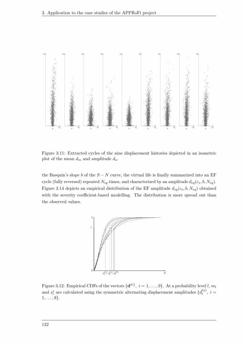
3. Application to the case studies of the APPRoFi project
Figure 3.11: Extracted cycles of the nine displacement histories depicted in an isometricplot of the mean dm and amplitude da.
the Basquin’s slope b of the S − N curve, the virtual life is finally summarized into an EF
cycle (fully reversed) repeated Neq times, and characterized by an amplitude deq(cs, b, Neq).
Figure 3.14 depicts an empirical distribution of the EF amplitude deq(cs, b, Neq) obtained
with the severity coefficient-based modelling. The distribution is more spread out than
the observed values.
Figure 3.12: Empirical CDFs of the vectors d′(i), i = 1, . . . , 9. At a probability level l, ml
and s∗l are calculated using the symmetric alternating displacement amplitudes d
′(i)l , i =
1, . . . , 9.
122

3.3. Blade support case study
Figure 3.13: CDF of the symmetric alternating amplitude for two values of the severitycoefficient. The dashed line depicts the mean CDF obtained for cs = 0. The solid linerepresents the CDF defined by cs = 2.
Figure 3.14: Empirical distribution of 1, 000 EF amplitudes deq at Neq cycles. The blackdots represent the EF amplitudes summarizing the nine displacement histories.
3.3.4 Numerical model
The EF cycle is applied to the numerical model simulating the elastic-plastic mechanical
behaviour of the blade support. The numerical model is characterized by a realization
ry, c1, c2 of the material properties and a geometry xg, which is considered as determin-
istic given that a preliminary sensitivity analysis has proven that its influence on structural
response is minor. The outputs of the numerical model are the elastic strain amplitude
ǫe(ry, c1, c2, xg, cs, b, Neq), the plastic strain amplitude ǫp(ry, c1, c2, xg, cs, b, Neq) and the
maximum stress σmax(ry, c1, c2, xg, cs, b, Neq).
123

3. Application to the case studies of the APPRoFi project
LMT’s multiparametric strategy and LATIN method [Relun, 2011] are employed to
reduce the CPU time of numerical model evaluations. For a single evaluation, the LATIN
solver appears to be competitive with the commercial code Abaqus [Relun, 2011]: the CPU
time using the LATIN method takes 800 seconds when considering a 141, 450 degrees of
freedom mesh and 48 time steps to solve the elastic-plastic problem, whereas Abaqus takes
1, 200 seconds (both computations are performed with a Intel Xeon W5650 processor at
2.6 Ghz - 6 cores). For succeeding numerical model evaluations, LMT’s multiparametric
strategy is seen to reduce the CPU time down to 40 seconds for small variations of the
material parameters.
A remote procedure call (see Figure 3.15) is set by Relun [2011] to enable communica-
tion between the probabilistic approach implemented by LaMI in Clermont-Ferrand, and
the efficient numerical model of LMT in Cachan. The AK-IS reliability method, imple-
mented for this case study, identifies the realization of the random variables, which, at the
current process stage, is relevant to compute. The realization is then automatically sent
to LMT’s numerical model, which, after evaluation, sends the values ǫe, ǫp, and σmax back
for fatigue calculation. No user intervention is required throughout the entire reliability
assessment.
Figure 3.15: Remote procedure call between LaMI’s methodology and LMT’s numericalmodel.
3.3.5 Reliability assessment
Table 3.9 recapitulates the random variables of the reliability problem. For a given
realization of these random variables, the Smith-Watson-Topper (SWT) stress σSWT =
σSWT(ry, c1, c2, cs, b, Neq) on the stabilized cycle is calculated using the different outputs
of the numerical model:
σSWT =√
E σmax (ǫp + ǫe) (3.7)
where E is the Young’s modulus. The performance function G compares the realization
of the SWT stress with the selected SWT strength rSWT(uf , Neq) at Neq cycles. As
mentioned previously, AK-IS is implemented to pilot the structural reliability analysis.
124

3.3. Blade support case study
Random variable Denomination Distribution
Ry Yield strength Lognormal
C1 Hardening parameter 1 Lognormal
C2 Hardening parameter 2 Lognormal
CS Severity coefficient Gaussian
Uf Isoprob. S − N curve Gaussian
Table 3.9: Random variables of the blade support case study.
3.3.6 Results
Table 3.10 reports the reliability results. FORM approximation requires 19 evaluations
of the performance function. Note that the finite difference approximation of the gradi-
ent does not require a new call to the numerical model for the component Uf , since
the calculation of the EF load does not depend on Uf . Hence, only 16 evaluations are
time-demanding. The Kriging procedure in AK-IS requires 11 additional computations
to classify a population of NIS = 104 points simulated in the vicinity of the approxim-
ated MPFP. The limit state seems to be linear as the failure probabilities obtained by
FORM and AK-IS are extremely similar. Within the frame of this case study, the Kriging
classification procedure validates the FORM approximation with only a few additional
evaluations.
Method NE P normf δ
FORM 16 1 -
AK-IS 27 1.01 2.5%
Table 3.10: Reliability results for the blade support case study. The failure probabilitiesare normalized to the FORM approximation.
The computational gain of AK-IS compared to crude IS is about 370 (10, 016/27).
Performing crude IS with the numerical model from Abaqus would require 139 days.
With AK-IS, the CPU time would drop to 9 hours (27 × 1, 200 seconds). Note that the
prediction step of AK-IS takes less than 3 seconds which is negligible in comparison with
the numerical model evaluation. Finally, by combining AK-IS with LMT’s methods, the
failure probability is assessed in 2.25 hours, given that the computational gain of the
LATIN + multiparametric strategy is 4 for this application. This case study proves that
combining parsimonious reliability methods with numerical strategies that reduce the CPU
time of succeeding model evaluations is of interest.
AK-IS enables the calculation of the direction cosines αi, i = Ry, C1, C2, CS , Uf of
125

3. Application to the case studies of the APPRoFi project
the vector P ⋆O. The values are reported in Table 3.11. The severity coefficient CS and
the S − N curve model are the most influent parameters on structural reliability. The
minor impact of the material random variables is due to the fact that the global structure
remains in the elastic domain.
Material Load Fatigue
−α2Ry
−α2C1
−α2C2
−α2CS
−α2Uf
−2.5 × 10⁻⁵ −1.6 × 10⁻⁵ −0.4 × 10⁻⁵ −0.270 −0.729
Table 3.11: Sensitivities −α2i of the different random variables for the blade support case
study.
3.4 Conclusion
In this chapter, the probabilistic approach outlined in Chapter 1 and the parsimonious
reliability methods of the AK-RM family introduced in Chapter 2 have successfully been
coupled to handle the two case studies submitted by SNECMA within the frame of the
APPRoFi project. The methodology has been completed with LMT’s numerical methods
with the aim of reducing the CPU time of succeeding model evaluations. For the blade
support case study, prompt reliability assessment has been proven possible despite time-
demanding model evaluations and small failure probability. Additionally, it has been
shown for these case studies that structural reliability in fatigue is mainly affected by the
load and the S − N curve, thus attention should be turned to their modellings and the
definition of tools for model selection.
126

Conclusion and future work
Conclusion
Fatigue in structural design is currently considered with deterministic approaches groun-
ded on the use of so-called safety factors. Although these deterministic approaches give
mostly satisfactory solutions, they often lead to over-design and are not sufficient to
provide the designer with the safety margin and the most influent design parameters on
structural reliability. To acquire this additional information, probabilistic approaches are
a possible alternative. The research as presented in this document represents a part of the
global probabilistic methodology developed in the ANR-funded project called APPRoFi,
and which aims at assessing the reliability of already designed structures within a short
space of time.
The first contribution of this research work is the definition of a general probabilistic
approach for fatigue analysis (Chapter 1). The proposed approach is an improvement on
the probabilistic Stress-stRength method [Thomas et al., 1999] which represents a prac-
tical engineering tool for assessing structural reliability in the context of fatigue. The main
limit of this method is the sensitivity of the failure probability estimate to the necessary
assumptions made on the distributions followed by the Stress and the stRength. Further-
more, the influences of random variables on structural reliability cannot be assessed since
these variables are carried either by the Stress or the stRength distribution. The proposed
approach overcomes these limits by keeping the different random variables separate from
each other. The advantages of this approach over the probabilistic Stress-stRength method
are demonstrated through an academic example. The approach is proven to enable the
assessment of a more accurate failure probability estimate, as well as a determination of
the random variables’ influences on structural reliability.
In the proposed approach, the failure probability can be assessed using sampling-based
reliability methods, but these are inapplicable in the case of a computationally demanding
numerical model since they require a substantial number of model evaluations. This thesis
thus proposes a family of reliability methods (Chapter 2) that are more parsimonious with
respect to the number of model evaluations. These methods named AK-RM (Active learn-
ing and Kriging-based Reliability Methods) represent improvements on various classical
sampling techniques through the use of a Kriging metamodel. They are based on a Kriging
127

3. Application to the case studies of the APPRoFi project
classification loop that iteratively identifies the model evaluation which should be carried
out to enhance the classification of a given population into its safe and failure subsets. The
first proposed reliability method is called AK-MCS and corresponds to the combination of
the Kriging classification loop with Monte Carlo Simulation. It is applicable to structural
reliability problems involving high non-linearity and disconnected domains of failure, but
the computational cost of its prediction step is observed to dramatically increase for fail-
ure probabilities below 10−3. Alternatives are thus proposed to consider smaller failure
probabilities. AK-MCSm is first suggested to take advantage of the possible monotony of
the performance function with respect to its random input variables. AK-IS is a second
alternative that consists in classifying a population simulated in the vicinity of the most
probable failure point. The computational cost of the Kriging procedure is greatly reduced,
but the approach relies on the hypothesis that the weight of the failure probability is well
located. Finally, AK-SS representing an improvement on Subset Simulation is proposed
as an intermediary method between the general AK-MCS and the more specific AK-IS.
The last point of this thesis is the application of the proposed probabilistic approach
to the case studies of the APPRoFi project (Chapter 3). In these case studies, the uncer-
tainties of the in-service loads, fatigue behaviour and material properties are statistically
modelled. The load uncertainty is examined using a mix strategy based on random per-
centages of occurrences, a random severity coefficient-based approach, and a parametric
modelling of Rainflow matrices. The uncertainty of the fatigue behaviour is considered
through the implementation of three probabilistic S − N curve models which are ranked
according to likelihood criteria and goodness-of-fit tests. Structural reliability assessment
and the determination of the importance factors are carried out using a method from the
AK-RM family. Given that the numerical model of the blade support case study is com-
putationally demanding, the probabilistic approach coupled with AK-IS is completed with
LMT’s numerical methods so that the time required to perform the structural reliability
analysis is reduced. The global methodology is proven to enable prompt failure probability
assessment. An important conclusion drawn from the application of the methodology to
the case studies is that structural reliability is essentially influenced by the load modelling
and the S − N curve model.
Future work
Following the conclusion on the application of the probabilistic approach to the particular
case studies, further investigations should be conducted in the modellings of the in-service
loads and S − N curves to enhance reliability assessment. Given that the fatigue be-
haviour of materials is relatively well known in comparison with the loads applied to
structures, attention should first be drawn to the stochastic modelling of the load with
other approaches such as stationary Gaussian processes [Pitoiset, 2001; Benasciutti and
Tovo, 2005] or Markovian processes [Mattrand and Bourinet, 2011; Mattrand, 2011].
128

3.4. Conclusion
In this research work, sensitivities are examined using importance factors. Global
sensitivity analysis such as Sobol’ indices is a step forward to a better understanding
of random structural response. These indices aim at determining the contribution of
each random variable to the variance of the structural response. They are commonly
estimated by means of Monte Carlo Simulation and consequently difficult to calculate
with time-demanding model evaluations. A Kriging metamodel can be used to estimate
them in a more efficient way, and, as proposed by Marrel et al. [2009], the full probabilistic
information held in the Kriging prediction can be considered to provide confidence intervals
on these indices. Other sensitivity measures such as Borgonovo’s [2007] may also be
calculated.
Safety factors are convenient to use, since they denote multiplicative coefficients to
apply to the load and resistance variables in the hope of obtaining a satisfactory design. In
comparison, the algorithmic procedure of probabilistic approaches seems disproportionate.
However, structural reliability analyses can be used to improve the concept of safety
factors. In fact, reliability-based calibration procedures [Gayton et al., 2004] may be
employed to set partial factors, which, when added to the design rule, confer the design
a given reliability objective. These factors are specific to the structures concerned and
consequently carry more meaning than traditional safety factors. They represent a relevant
direction to consider in order to settle probabilistic approaches in design offices.
The research as presented in this document is concerned with the problem of reliability
assessment, but uncertainties can also be considered in the design optimization process
with the purpose of devising robust and cost-effective structures. Such an advanced process
is commonly referred to as reliability-based design optimization. Finding the optimal set of
design parameters that minimizes some cost function while satisfying a reliability objective
is a problem of obvious interest in mechanical engineering. Nevertheless, it represents a
significant computational effort, given that a reliability problem needs to be solved for
each set of the design parameters. Following the recent advances in this field involving
Kriging [Bichon et al., 2009; Dubourg, 2011; Dubourg et al., 2011], the AK-RM family
may be adapted to tackle such analyses.
129

3. Application to the case studies of the APPRoFi project
130

Bibliography
AFCEN. Règles de Conception et de Construction des Matériels des Ilots Nucléaires,
(RCC-M), 2000.
AFNOR. A03-405, Metal products - Fatigue testing - Data statistical processing, 1991.
AFNOR. A03-406, Metal products - Fatigue under variable amplitude loading - The
Rainflow method of cycle counting, 1993.
H. Akaike. A new look at the statistical model identification. IEEE Transactions on
Automatic Control, 19(6):716–723, 1974.
C. Amzallag, J. P. Gerey, J.-L. Robert, and J. Bahuaud. Standardization of the rainflow
counting method for fatigue analysis. International Journal of Fatigue, 16(4):287–293,
1994.
S.-K. Au and J. L. Beck. Estimation of small failure probabilities in high dimensions by
Subset Simulation. Probabilistic Engineering Mechanics, 16(4):263–277, 2001.
F. Bastenaire. Etude statistique et physique de la dispersion des résistances et des endur-
ances à la fatigue. PhD thesis, Faculté des Sciences de l’université de Paris, 1960.
J. Bect, D. Ginsbourger, L. Li, V. Picheny, and E. Vazquez. Sequential design of computer
experiments for the estimation of a probability of failure. Statistics and Computing, 22:
773–793, 2011.
D. Benasciutti and R. Tovo. Spectral methods for lifetime prediction under wide-band
stationary random processes. International Journal of Fatigue, 27(8):867–877, 2005.
P. Bernard and M. Fogli. Une méthode de Monte Carlo performante pour le calcul de la
probabilité de ruine. Construction Métallique, 4:23–29, 1987.
B. J. Bichon, M. S. Eldred, L. P. Swiler, S. Mahadevan, and J. M. McFarland. Efficient
Global Reliability Analysis for nonlinear implicit performance functions. AIAA Journal,
46:2459–2468, 2008.
131

Bibliography
B. J. Bichon, S. Mahadevan, and M. Eldred. Reliability-based design optimization using
efficient global reliability analysis. In 50th AIAA/ASME/ASCE/ AHS/ASC Structures,
Structural Dynamics, and Materials Conference, Palm Springs, California, USA, May
2009.
B. J. Bichon, J. M. McFarland, and S. Mahadevan. Efficient surrogate models for reliability
analysis of systems with multiple failure modes. Reliability Engineering & System Safety,
96(10):1386–1395, 2011.
A. Bignonnet and H.-P. Lieurade. Reliability application in the industry of the reliability
approach in fatigue design: a CETIM multipartner project. In 2nd Fatigue Design,
Senlis, France, November 2007. CETIM.
A. Bignonnet and J.-J. Thomas. Approche fiabiliste en conception automobile. In SF2M
- Journées de Printemps, Paris, France, May 2004.
A. Bignonnet, H.-P. Lieurade, I. Hunter, F. Lefebvre, A. Carcan, E. Babaud, and Mar-
quand D. Escoffier, J.-C. The reliability approach in fatigue design: DEFFI project. In
3rd Fatigue Design, Senlis, France, November 2009. CETIM.
G. Blatman and B. Sudret. An adaptive algorithm to build up sparse polynomial chaos
expansions for stochastic finite element analysis. Probabilistic Engineering Mechanics,
25(2):183–197, 2010.
B. Boniface. Modélisation thermo-mécanique et fiabilité des échangeurs réacteurs en car-
bure de silicium. PhD thesis, Université de Toulouse, 2010.
J. D. Booker, M. Raines, and K. G. Swift. Designing Capable and Reliable Products,
chapter Stress Strength Interference (SSI) analysis, pages 176–191. Butterworth-
Heinemann, 2001.
E. Borgonovo. A new uncertainty importance measure. Reliability Engineering & System
Safety, 92(6):771–784, 2007.
P.-A. Boucard and L. Champaney. A suitable computational strategy for the parametric
analysis of problems with multiple contact. International Journal for Numerical Methods
in Engineering, 57(9):1259–1281, 2003.
J.-M. Bourinet, F. Deheeger, and M. Lemaire. Assessing small failure probabilities by
combined Subset Simulation and Support Vector Machines. Structural Safety, 33(6):
343–353, 2011.
C. G. Bucher and U. Bourgund. A fast and efficient response surface approach for struc-
tural reliability problems. Structural Safety, 7(1):57–66, 1990.
132

Bibliography
J.-L. Chaboche. Constitutive equations for cyclic plasticity and cyclic viscoplasticity.
International Journal of Plasticity, 5(3):247–302, 1989. ISSN 0749-6419.
D. D. Cox and S. John. SDO: A Statistical Method for Global Optimization. In M. N.
Alexandrov and M. Y. Hussaini, editors, Multidisciplinary Design Optimization: State-
of-the-Art, pages 315–329. Siam, Philadelphia, 1997.
R. B. D’Agostino and M. A. Stephens. Goodness-Of-Fit Techniques. 1986.
P. K. Das and Y. Zheng. Cumulative formation of response surface and its use in reliability
analysis. Probabilistic Engineering Mechanics, 15(4):309–315, 2000.
E. De Rocquigny. Structural reliability under monotony: Properties of FORM, simulation
or response surface methods and a new class of Monotonous Reliability Methods (MRM).
Structural Safety, 31(5):363–374, 2009.
G. Defaux, E. Meister, and M. Pendola. Mécanique probabiliste et intégrité des cuves des
réacteurs nucléaires. In 6th Journées nationales de la fiabilité, Toulouse, France, March
2010.
A. Der Kiureghian and T. Dakessian. Multiple design points in first and second-order
reliability. Structural Safety, 20(1):37–49, 1998.
A. Der Kiureghian and P. L. Liu. Structural reliability under incomplete probability
information. Journal of Engineering Mechanics, 112(1):85–104, 1986.
O. Ditlevsen and H. O. Madsen. Structural Reliability Methods. John Wiley & Sons, 1996.
O. Ditlevsen, P. Bjerager, R. Olesen, and A. M. Hasofer. Directional Simulation in Gaus-
sian processes. Probabilistic Engineering Mechanics, 3(4):207–217, 1988.
S. D. Downing and D. F. Socie. Simple rainflow counting algorithms. International Journal
of Fatigue, 4(1):31–40, 1982.
V. Dubourg. Adaptive surrogate models for reliability analysis and reliability-based design
optimization. PhD thesis, Université Blaise Pascal – Clermont II, 2011.
V. Dubourg, B. Sudret, and J.-M. Bourinet. Reliability-based design optimization using
Kriging surrogates and subset simulation. Structural and Multidisciplinary Optimiza-
tion, 44(5):673–690, 2011.
A. Dumas, B. Echard, N. Gayton, and O. Rochat. AK-ILS: an Active learning method
based on Kriging for the Inspection of Large Surfaces. In 3rd International Conference
on Surface Metrology, Annecy, France, March 2012.
133

Bibliography
A. Dumas, B. Echard, N. Gayton, O. Rochat, J.-Y. Dantan, and S. Van Der Veen. AK-
ILS: an Active learning method based on Kriging for the Inspection of Large Surfaces.
Precision Engineering, 37(1):1–9, 2013.
B. Echard, N. Gayton, and M. Lemaire. Reliability assessment of structures subjected to
fatigue failure using Kriging methods. In 3rd Fatigue Design, Senlis, France, November
2009. CETIM.
B. Echard, N. Gayton, and M. Lemaire. Structural reliability assessment using Kriging
metamodel and Monte Carlo Simulation. In D. Straub, L. Esteva, and M. Faber, editors,
Reliability and Optimization of Structural Systems, Proceedings of the 15th IFIP WG
7.5 Working Conference, pages 61–68. CRC Press, Munich, Germany, 2010a.
B. Echard, N. Gayton, and M. Lemaire. Kriging based Monte Carlo Simulation to compute
the probability of failure efficiently: AK-MCS method. In 6th Journées nationales de la
fiabilité, Toulouse, France, March 2010b.
B. Echard, N. Gayton, and M. Lemaire. AK-MCS: An Active learning reliability method
combining Kriging and Monte Carlo Simulation. Structural Safety, 33(2):145–154,
2011a.
B. Echard, N. Gayton, and M. Lemaire. A Kriging improvement of the Monte Carlo
Simulation: AK-MCS method. In M. Faber, J. Köhler, and K. Nishijima, editors,
Applications of Statistics and Probability in Civil Engineering, Proceedings of the 11th
International Conference on Applications of Statistics and Probability in Civil Engin-
eering, pages 679–686. CRC Press, Zurich, Switzerland, August 2011b.
B. Echard, N. Gayton, M. Lemaire, M. Afzali, A. Bignonnet, P.-A. Boucard, G. Defaux, J.-
L. Dulong, A. Ghouali, F. Lefebvre, and A. Pyre. Reliability assessment of an aerospace
component subjected to fatigue loadings: APPRoFi project. In 4th Fatigue Design,
Senlis, France, November 2011c. CETIM.
B. Echard, N. Gayton, M. Lemaire, and N. Relun. A combined Importance Sampling and
Kriging reliability method for small failure probabilities with time-demanding numerical
models. Reliability Engineering & System Safety, in press, 2012.
FEM. 1.001 - Règles de calcul des appareils de levage, 1998.
M. Ferlin, A. Pyre, F. Lefebvre, S. Oriol, and A. Bignonnet. DEFFI project for a new
concept of fatigue design in the aerospace domain. In 50th AIAA/ASME/ASCE/ AH-
S/ASC Structures, Structural Dynamics, and Materials Conference, Palm Springs, Cali-
fornia, USA, May 2009.
134
Bibliography
D. E. Finkel. DIRECT Optimization Algorithm User Guide. Center for Research in
Scientific Computation, North Carolina State University, March 2003.
R. A. Fisher. Statistical methods for research workers. Oliver & Boyd, Edinburgh, 1950.
J. M. Gablonsky. Modifications of the DIRECT algorithm. PhD thesis, North Carolina
State University, 2001.
N. Gayton and B. Echard. AK-RM : une nouvelle famille de méthodes de simulation basée
sur le krigeage. In 7th Journées nationales de la fiabilité, Chambéry, France, June 2012.
N. Gayton, J.-M. Bourinet, and M. Lemaire. CQ2RS: a new statistical approach to the
response surface method for reliability analysis. Structural Safety, 25(1):99–121, 2003.
N. Gayton, A. Mohamed, J. D. Sorensen, M. Pendola, and M. Lemaire. Calibration
methods for reliability-based design codes. Structural Safety, 26(1):91–121, 2004.
N. Gayton, M. Afzali, A. Bignonnet, P.-A. Boucard, G. Defaux, J.-L. Dulong, B. Echard,
A. Ghouali, F. Lefebvre, M. Lemaire, M. Masmoudi, A. Notin, D. Néron, A. Ostmane,
A. Pyre, and N. Relun. APPRoFi Project: A new approach for the reliability assessment
of structures subjected to fatigue. In 4th Fatigue Design, Senlis, France, November 2011.
CETIM.
G. Genet. A statistical approach to multi-input equivalent fatigue loads for the durability
of automotive structures. PhD thesis, Chalmers, Göteborg University, 2006.
R. G. Ghanem and P. D. Spanos. Stochastic Finite Elements: A Spectral Approach.
Springer, Berlin, 1991.
C. J. Gil Bellosta. Package ‘ADGofTest’: Anderson-Darling GoF test with p-value calcu-
lation based on Marsaglia’s 2004 paper ‘Evaluating the Anderson-Darling Distribution’,
2011. URL http://cran.r-project.org/web/packages/ADGofTest/ADGofTest.pdf.
Z. Guédé. Approche probabiliste de la durée de vie des structures soumises à la fatigue
thermique. PhD thesis, Université Blaise Pascal – Clermont II, 2005.
Z. Guédé, B. Sudret, and M. Lemaire. Life-time reliability based assessment of structures
submitted to thermal fatigue. International Journal of Fatigue, 29(7):1359–1373, 2007.
S. Hanaki, M. Yamashita, H. Uchida, and M. Zako. On stochastic evaluation of S-N data
based on fatigue strength distribution. International Journal of Fatigue, 32(3):605–609,
2010.
A. M. Hasofer and N. C. Lind. Exact and invariant second moment code format. Journal
of Engineering Mechanics, 100:111–121, 1974.
135

Bibliography
W. K. Hastings. Monte Carlo sampling methods using Markov chains and their applica-
tions. Biometrika, 57(1):97–109, 1970.
J. E. Hurtado. An examination of methods for approximating implicit limit state functions
from the viewpoint of statistical learning theory. Structural Safety, 26(3):271–293, 2004.
D. R. Jones, C. D. Perttunen, and B. E. Stuckman. Lipschitzian optimization without the
Lipschitz constant. Journal of Optimization Theory and Applications, 79(1):157–181,
1993.
D. R. Jones, M. Schonlau, and W. J. Welch. Efficient Global Optimization of expensive
black-box functions. Journal of Global Optimization, 13(4):455–492, 1998.
D. Karaboga. An idea based on honey bee swarm for numerical optimization. Technical Re-
port TECHNICAL REPORT-TR06, Erciyes University, Engineering Faculty, Computer
Engineering Department, 2005. URL http://mf.erciyes.edu.tr/abc/publ.htm.
D. Karaboga and B. Basturk. A powerful and efficient algorithm for numerical function
optimization: artificial bee colony (ABC) algorithm. Journal of Global Optimization,
39:459–471, 2007.
I. Kaymaz. Application of Kriging method to structural reliability problems. Structural
Safety, 27(2):133–151, 2005.
M. C. Kennedy, C. W. Anderson, S. Conti, and A. O’Hagan. Case studies in Gaussian
process modelling of computer codes. Reliability Engineering & System Safety, 91(10-
11):1301–1309, 2006. The Fourth International Conference on Sensitivity Analysis of
Model Output (SAMO 2004).
D. Krige. A statistical approach to some basic mine valuation problems on the Witwater-
srand. Journal of the Chemical, Metallurgical and Mining Society of South Africa, 52
(6):119–139, 1951.
H. J. Kushner. A new method of locating the maximum of an arbitrary multipeak curve
in the presence of noise. Journal of Basic Engineering, 86:97–106, 1964.
P. Ladevèze. Nonlinear Computational Structural Methods: New Approaches and Non-
Incremental Methods of Calculation. Mechanical Engineering Series. Springer-Verlag,
1999.
C. Lalanne. Mechanical Vibration and Shock: Fatigue Damage, volume 4. Hermes Penton
Ltd, 2002.
R. Lebrun and A. Dutfoy. An innovating analysis of the Nataf transformation from the
copula viewpoint. Probabilistic Engineering Mechanics, 24(3):312–320, 2009.
136

Bibliography
F. Lefebvre, M. Ferlin, A. Pyre, A. Ghouali, S. Oriol, J. El Maghnouji, and A. Bignonnet.
Reliability approach in fatigue design for aerospace industry. In 3rd Fatigue Design,
Senlis, France, November 2009. CETIM.
M. Lemaire. Structural reliability. ISTE, 2009.
J. Lemaitre, J.-L. Chaboche, A. Benallal, and R. Desmorat. Mécanique des matériaux
solides. 3rd edition, 2009.
L. Li, J. Bect, and E. Vazquez. A numerical comparison of kriging-based sequen-
tial strategies for estimating a probability of failure. In M. Faber, J. Köhler, and
K. Nishijima, editors, Applications of Statistics and Probability in Civil Engineering,
Proceedings of the 11th International Conference on Applications of Statistics and Prob-
ability in Civil Engineering. CRC Press, Zurich, Switzerland, August 2011.
S. N. Lophaven, H. B. Nielsen, and J. Sondergaard. DACE, a Matlab Kriging Toolbox,
Version 2.0. Technical Report IMM-TR-2002-12, Technical University of Denmark,
2002a. URL http://www2.imm.dtu.dk/~hbn/dace/.
S. N. Lophaven, H. B. Nielsen, and J. Sondergaard. Aspects of the Matlab Toolbox DACE.
Technical Report IMM-REP-2002-13, Technical University of Denmark, 2002b. URL
http://www2.imm.dtu.dk/~hbn/dace/.
X. Luo, X. Li, J. Zhou, and T. Cheng. A Kriging-based hybrid optimization algorithm for
slope reliability analysis. Structural Safety, 34(1):401–406, 2012.
A. Marrel, B. Iooss, B. Laurent, and O. Roustant. Calculations of Sobol’ indices for the
Gaussian process metamodel. Reliability Engineering & System Safety, 94(3):742–751,
2009.
G. Marsaglia and J. Marsaglia. Evaluating the Anderson-Darling distribution. Journal of
Statistical Software, 9(2):1–5, 2004. URL http://www.jstatsoft.org/v09/i02.
G. Matheron. The intrinsic random functions and their applications. Advances in Applied
Probability, 5(3):439–468, 1973.
M. Matsuishi and T. Endo. Fatigue of metals subjected to varying stress. In Japan Society
of Mechanical Engineering, Jukvoka, Japan, 1968.
C. Mattrand. Approche probabiliste de la tolérance aux dommages - Application au domaine
aéronautique. PhD thesis, Université Blaise Pascal – Clermont II, 2011.
C. Mattrand and J.-M. Bourinet. Random load sequences and stochastic crack growth
based on measured load data. Engineering Fracture Mechanics, 78(17):3030 – 3048,
2011.
137

Bibliography
M. McKay, R. Beckman, and W. Conover. A comparison of three methods for selecting
values of input variables in the analysis of output from a computer code. Technometrics,
21(2):239–245, 1979.
R.E. Melchers. Radial importance sampling for structural reliability. Journal of Engin-
eering Mechanics, 116(1):189–203, 1990.
N. Metropolis, A. W. Rosenbluth, M. N. Rosenbluth, A. H. Teller, and E. Teller. Equation
of state calculations by fast computing machines. The Journal of Chemical Physics, 21
(6):1087–1092, 1953.
M. A. Miner. Cumulative damage in fatigue. Journal of Applied Mechanics, 12:159–164,
1945.
F. Morel, J. Mercier, G. Catherin, A. Bignonnet, J. Petit, and N. Ranganathan. Analyse
du comportement en fatigue de composants mécaniques par l’approche du chargement
équivalent. In Journées de printemps: Sollicitations de service et comportement en
fatigue, Paris, France, May 1993. SF2M.
M. Nagode. rebmix: An R Package for continuous and discrete finite mixture models,
2012. URL http://cran.r-project.org/web/packages/rebmix/index.html.
M. Nagode and M. Fajdiga. A general multi-modal probability density function suitable for
the Rainflow ranges of stationary random processes. International Journal of Fatigue,
20(3):211–223, 1998.
M. Nagode and M. Fajdiga. An improved algorithm for parameter estimation suitable for
mixed Weibull distributions. International Journal of Fatigue, 22:75–80, 2000.
M. Nagode and M. Fajdiga. An alternative perspective on the mixture estimation problem.
Reliability Engineering & System Safety, 91:388–397, 2006.
M. Nagode and M. Fajdiga. The REBMIX algorithm for the multivariate finite mixture
estimation. Communications in Statistics - Theory and Methods, 40(11):2022–2034,
2011a.
M. Nagode and M. Fajdiga. The REBMIX algorithm for the univariate finite mixture
estimation. Communications in Statistics - Theory and Methods, 40(5):876–892, 2011b.
M. Nagode, J. Klemenc, and M. Fajdiga. Parametric modelling and scatter prediction of
rainflow matrices. International Journal of Fatigue, 23(6):525–532, 2001.
A. Nataf. Détermination des distributions dont les marges sont données. Comptes Rendus
Académie des Sciences, 225:42–43, 1962.
138

Bibliography
NIST/SEMATECH. e-Handbook of Statistical Methods: Anderson-Darling Test. URL
http://www.itl.nist.gov/div898/handbook/eda/section3/eda35e.htm.
A. O’Hagan. Bayesian analysis of computer code outputs: a tutorial. Reliability Engineer-
ing & System Safety, 91(10-11):1290–1300, 2006. The Fourth International Conference
on Sensitivity Analysis of Model Output (SAMO 2004).
F. Perrin. Prise en compte des données expérimentales dans les modèles probabilistes pour
la prévision de la durée de vie des structures. PhD thesis, Université Blaise Pascal –
Clermont II, 2008.
V. Picheny, D. Ginsbourger, O. Roustant, R. T. Haftka, and N.-H. Kim. Adaptive designs
of experiments for accurate approximation of a target region. Journal of Mechanical
Design, 132(7):071008, 2010.
X. Pitoiset. Méthodes spectrales pour une analyse en fatigue des structures métalliques
sous chargements aléatoires multiaxiaux. PhD thesis, Université Libre de Bruxelles,
2001.
R. Rackwitz. Reliability analysis - a review and some perspectives. Structural Safety, 23
(4):365–395, 2001.
R. Rackwitz and B. Fiessler. Structural reliability under combined random load sequences.
Computers & Structures, 9(5):489–494, 1978.
M. R. Rajashekhar and B. R. Ellingwood. A new look at the response surface approach
for reliability analysis. Structural Safety, 12(3):205–220, 1993.
P. Ranjan, D. Bingham, and G. Michailidis. Sequential experiment design for contour
estimation from complex computer codes. Technometrics, 50(4):527–541, 2008.
N. Relun. Stratégie multiparamétrique pour la conception robuste en fatigue. PhD thesis,
Ecole Normale Supérieure de Cachan, 2011.
J.-L. Robert. Dimensionnement en fatigue des pièces mécaniques. Lectures notes in Master
Ingénierie Mécanique et Civile, Université Blaise Pascal – Clermont II, 2009.
V. J. Romero, L. P. Swiler, and A. A. Giunta. Construction of response surfaces based
on progressive-lattice-sampling experimental designs with application to uncertainty
propagation. Structural Safety, 26(2):201–219, 2004.
J. Sacks, S. B. Schiller, and W. J. Welch. Design for computer experiment. Technometrics,
31(1):41–47, 1989.
T. J. Santner, B. J. Williams, and W. I. Notz. The Design and Analysis of Computer
Experiments. New York, 2003.
139

Bibliography
G. Saporta. Probabilités, analyse des données et statistique. Editions Technip, 2nd edition,
2006.
L. Schueremans and D. Van Gemert. Benefit of splines and neural networks in simulation
based structural reliability analysis. Structural Safety, 27(3):246–261, 2005.
G. Schwarz. Estimating the dimension of a model. The Annals of Statistics, 6(2):461–464,
1978.
K. N. Smith, P. Watson, and T. H. Topper. A stress-strain function for the fatigue of
metals. Journal of Materials, 5(4):767–778, 1970.
B. Sudret. Fatigue of materials and structures, chapter 5: Probabilistic design of structures
submitted to fatigue, pages 223–263. Wiley & Sons, 2011.
B. Sudret and A. Der Kiureghian. Comparison of finite element reliability methods. Prob-
abilistic Engineering Mechanics, 17(4):337–348, 2002.
S. Suresh. Fatigue of materials. Cambridge University Press, 2nd edition, 1998.
T. Svensson. Prediction uncertainties at variable amplitude fatigue. International Journal
of Fatigue, 19(93):295–302, 1997.
J.-J. Thomas, G. Perroud, A. Bignonnet, and D. Monnet. Fatigue design and reliability
in the automotive industry. In G. Marquis and J. Solin, editors, Fatigue Design and
Reliability, volume 23 of European Structural Integrity Society, pages 1–11. Elsevier,
1999.
A. Törn and A. Zilinskas. Global optimization. Lecture Notes in Computer Science, 350,
1989.
R. Tovo. On the fatigue reliability evaluation of structural components under service
loading. International Journal of Fatigue, 23(7):587–598, 2001.
D. Veldkamp. Chances in wind energy - a probabilistic approach to wind turbine fatigue
design. PhD thesis, Delft University of Technology: TU Delft, 2006.
P. H. Waarts. Structural reliability using finite element methods: an appraisal of DARS
(Directional Adaptive Response Surface Sampling). PhD thesis, TU Delft, 2000.
Y. Zhang and A. Der Kiureghian. Two improved algorithms for reliability analysis. In
R. Rackwitz, G. Augusti, and A. Bori, editors, Reliability and optimization of structural
systems, Proceedings of the 6th IFIP WG7.5 Working Conference on reliability and
optimization of structural systems, Assisi, Italy, 1995. Chapman & Hall.
140

A List of abbreviations
AIC Akaike information criterion
AK-ILS Active learning and Kriging-based method for inspection of large surfaces
AK-IS Active learning and Kriging-based importance sampling
AK-MCS Active learning and Kriging-based Monte Carlo simulation
AK-MCSm Active learning and Kriging-based Monte Carlo simulation under monotony
AK-RM Active learning and Kriging-based reliability methods
AK-SS Active learning and Kriging-based subset simulation
ANR Agence nationale de la recherche
APPRoFi Approche mécano-probabiliste pour la conception robuste en fatigue
BIC Bayesian information criterion
BLUP Best linear unbiased predictor
CA Constant amplitude
CDF Cumulative distribution function
DEFFI Démarche fiabiliste de conception en fatigue pour l’industrie
DOE Design of numerical experiments
EF Equivalent fatigue
EFF Expected feasibility function
EGRA Efficient global reliability analysis
FORM First order reliability method
GOF Goodness-Of-Fit
HLRF Hasofer-Lind-Rackwitz-Fiessler algorithm
IS Importance sampling
MCS Monte Carlo simulation
MCSm Monte Carlo simulation under monotony
ML Maximum likelihood
MPFP Most probable failure point
PDF Probability density function
SS Subset simulation
SSI Stress-strength interference
SWT Smith-Watson-Topper
VA Variable amplitude
141

A. List of abbreviations
142

B List of notations
B.1 General notations
V Column vector
Vt Line vector
Vi ith component of V
M Matrix
. Estimation
. Approximation
Prob Probability
B.2 Deterministic mechanical values
Rm Tensile strength
N Number of cycles to failure
b Basquin’s slope, Eqn.(1.3)
B Fatigue strength coefficient in Basquin’s relation, Eqn.(1.3)
σ(t), F (t) Stress, force history
σm, Fm Mean value of a cycle
σa, Fa Amplitude value of a cycle
σmin, Fmin Minimum value of a cycle
σmax, Fmax Maximum value of a cycle
∆σ, ∆F Range of a cycle
σ′a, F ′
a Symmetric alternating amplitude of a cycle
R Stress or load ratio
σeq, Feq Amplitude of the equivalent fatigue (EF) cycle (often fully reversed)
Neq Number of times an equivalent fatigue (EF) cycle is repeated
143

B. List of notations
B.3 Random values
B.3.1 Scalar and statistical values
X or X(ω) Random variable
x Realization of the random variable X
µX Mean of the random variable X
σX Standard deviation of the random variable X
δX Coefficient of variation of the random variable X
N (µX , σ2X) Gaussian distribution with mean µX and variance σ2
X
fX Probability density function (PDF) of the random variable X
FX Cumulative distribution function (CDF) of the random variable X
φ Standard Gaussian probability density function (PDF)
Φ Standard Gaussian cumulative distribution function (CDF)
mX Empirical mean of the random variable X
s∗X Unbiased standard deviation estimate of the random variable X
B.3.2 Vectorial values
X Random vector
x Realization of the random vector X
U Random vector of standard Gaussian variables
u Realization of the standard Gaussian vector U
P Population of points
fX Joint probability density function (PDF) of the random vector X
φn n-dimensional standard Gaussian probability density function (PDF)
B.3.3 Space notation and random functions
X n n-dimensional physical space
Un n-dimensional standard space
O Origin of the standard space
S Safe domain
F Failure domain
G(X) Performance function of the random vector X
H(U) Performance function in standard space Un
144

B.3. Random values
B.3.4 Random mechanical values
S Stress distribution
R StRength distribution at Neq cycles
Uf Random isoprobability S − N curve
Xl Random load parameters
Xg Random geometry parameters
Xm Random material parameters
B.3.5 Kriging values
µH(u) Kriging mean at a point u
σ2H
(u) Kriging variance at a point u
U(u) Learning function at a point u
u Point leading to the smallest value of the learning function U
NE Number of numerical model (or performance function) evaluations
B.3.6 Reliability analysis products
Pf Failure probability
Pf Failure probability estimator or estimate, depending on the context
Pf Failure probability estimate obtained with a metamodel
P f Reliability objective, i.e. targeted failure probability
δ Coefficient of variation of the failure probability estimator
P ⋆ Most probable failure point (MPFP)
β Hasofer-Lind reliability index
αi Direction cosines of the ith random variable
EpiElasticities of the Hasofer-Lind reliability index with respect to the parameter p
of the ith random variable
145

B. List of notations
146

C Parametric modelling of the load
for the blade support case study
In Section 3.3.3.2, the load applied to the blade support case study is modelled with the
symmetric alternating amplitude d′ and a random severity coefficient CS . An alternative
approach inspired by the parametric modelling method outlined in Section 1.3.4.2 and
developed after the APPRoFi project is proposed in this appendix.
Selection of the symmetric alternating displacement amplitude’s CDF
The proposed approach aims at modelling the CDF of the symmetric alternating displace-
ment amplitude for which only 9 vectors d′(i), i = 1, . . . , 9 are observed (see Figure
3.12). The ‘rebmix’ package for R [Nagode and Fajdiga, 2011a,b] is used to determine
whether multiple component distributions are required to model each vector d′(i). Mix-
tures of Weibull or lognormal distributions are assumed, and BIC is used to determine the
most adequate number z of components for each vector. The number of component distri-
butions is reported in Table C.1. A single Weibull distribution is found to be appropriate
for eight vectors. Only the first vector is better modelled with a mixture of two Weibull
distributions. For lognormal models, a single distribution is seen as relatively sufficient.
Following these results, it seems acceptable to consider that a vector d′(i) is adequately
modelled with a single distribution.
Given that z is now set to 1, the most satisfactory distribution between Weibull and
lognormal must be selected. For that, Table C.2 and Table C.3 report AIC, BIC and the
p-values of Kolmogorov-Smirnov tests. According to AIC and BIC (the lower, the better),
the Weibull distribution is the most appropriate. Its p-values are also considerably higher
than those of the lognormal distribution. The Weibull hypothesis is not rejected at a
5% significance level for five vectors (#2, 6, 7, 8, 9), and the p-values of the four other
vectors remain relatively high (≈ 1%) despite the large data set of cycles extracted in
each history. The Weibull model is thus selected as the distribution of the symmetric
alternating displacement amplitude.
147

C. Parametric modelling of the load for the blade support case study
Modelling of the scatter observed in the CDF’s parameters
The nine Weibull distributions fitting the vectors d′(i), i = 1, . . . , 9 provide nine ob-
servations of the random scale λ(ω) and shape κ(ω) parameters. Statistical models are
inferred by ML estimation for λ(ω) and κ(ω). Table C.4 shows that Gaussian, lognormal
and Weibull models have very similar AIC, BIC and p-values. In this study, λ(ω) is con-
sidered as a Weibull variable, since the AIC and BIC values are the lowest. Given that
the support of the Weibull distribution is R+, no truncation at 0 is required for λ(ω).
Concerning the shape parameter κ(ω), it is assumed that its realizations cannot be
below 1 which represents the bound between two drastically different Weibull PDF shapes
(remember that a Weibull distribution with κ = 1 corresponds to the exponential PDF).
Table C.5 shows that the Gaussian, lognormal and Weibull models have close AIC, BIC
and p-values. κ(ω) is defined as a Weibull random variable for its slightly better AIC and
BIC values.
For a given realization κ, λ of the Weibull distribution’s parameters, the Weibull
CDF of the symmetric alternating displacement amplitude is built, and a virtual life is
obtained by discretizing the CDF into Nf regularly-distributed probability levels. The
amplitudes associated with the different probability levels are calculated using the inverse
Weibull CDF that reads:
F −1(l) = λ (− ln(1 − l))1κ (C.1)
This function is not defined at the probability level l = 1. Therefore, a third random
variable is necessary to define the highest symmetric alternating displacement amplitude
observed in the virtual life. This random variable is denoted by Dmax and assumed to
be Weibull distributed, as Table C.6 shows that it is the model that best fits the nine
maximum amplitudes observed in the vectors d′(i), i = 1, . . . , 9.
Comparison with the severity coefficient-based model
A virtual life, i.e. a vector d′(κ, λ, dmax), is generated by selecting a realization κ, λ, dmax.
Using the Basquin’s slope b of the S −N curve, the life is summarized into an EF cycle re-
peated Neq times and characterized by its amplitude deq(κ, λ, dmax, b, Neq). Figure C.1(a)
depicts an empirical distribution of the EF amplitude obtained with the parametric model
presented in this appendix. Figure C.1(b) illustrates an empirical distribution which is
derived from the severity coefficient-based model exposed in Section 3.3.3.2. The EF
amplitude is seen to be less scattered with the parametric method. Using this model in a
structural reliability analysis would then lead to a smaller failure probability.
148

Vector # z Weibull z lognormal
1 2 1
2 1 2
3 1 2
4 1 2
5 1 2
6 1 1
7 1 1
8 1 1
9 1 1
Table C.1: Determination using BIC of the number z of component distributions (Weibullor lognormal) required to model each vector d′(i).
Vector #Weibull
AIC BIC p-value
1 −7573 −7562 0.013
2 −8622 −8611 0.621
3 −8863 −8852 0.010
4 −8664 −8653 0.018
5 −9157 −9146 0.009
6 −7831 −7820 0.346
7 −8083 −8073 0.281
8 −7638 −7627 0.768
9 −8381 −8370 0.352
Table C.2: Measures of the relative goodness of fit of the Weibull distribution to the ninevectors d′(i), i = 1, . . . , 9.
149
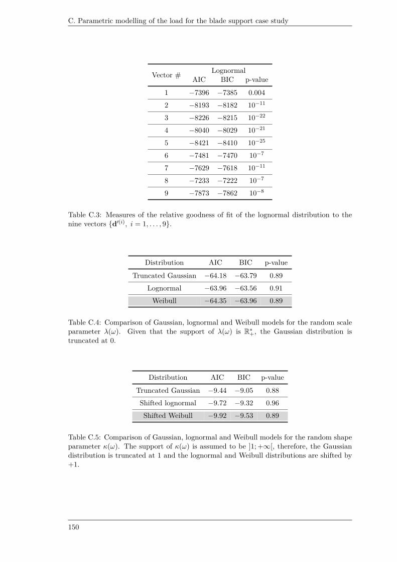
C. Parametric modelling of the load for the blade support case study
Vector #Lognormal
AIC BIC p-value
1 −7396 −7385 0.004
2 −8193 −8182 10−11
3 −8226 −8215 10−22
4 −8040 −8029 10−21
5 −8421 −8410 10−25
6 −7481 −7470 10−7
7 −7629 −7618 10−11
8 −7233 −7222 10−7
9 −7873 −7862 10−8
Table C.3: Measures of the relative goodness of fit of the lognormal distribution to thenine vectors d′(i), i = 1, . . . , 9.
Distribution AIC BIC p-value
Truncated Gaussian −64.18 −63.79 0.89
Lognormal −63.96 −63.56 0.91
Weibull −64.35 −63.96 0.89
Table C.4: Comparison of Gaussian, lognormal and Weibull models for the random scaleparameter λ(ω). Given that the support of λ(ω) is R
∗+, the Gaussian distribution is
truncated at 0.
Distribution AIC BIC p-value
Truncated Gaussian −9.44 −9.05 0.88
Shifted lognormal −9.72 −9.32 0.96
Shifted Weibull −9.92 −9.53 0.89
Table C.5: Comparison of Gaussian, lognormal and Weibull models for the random shapeparameter κ(ω). The support of κ(ω) is assumed to be ]1; +∞[, therefore, the Gaussiandistribution is truncated at 1 and the lognormal and Weibull distributions are shifted by+1.
150
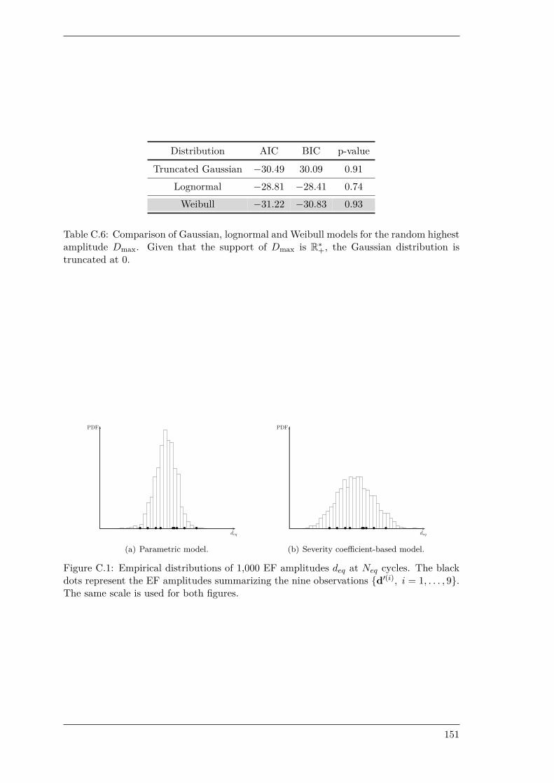
Distribution AIC BIC p-value
Truncated Gaussian −30.49 30.09 0.91
Lognormal −28.81 −28.41 0.74
Weibull −31.22 −30.83 0.93
Table C.6: Comparison of Gaussian, lognormal and Weibull models for the random highestamplitude Dmax. Given that the support of Dmax is R
∗+, the Gaussian distribution is
truncated at 0.
(a) Parametric model. (b) Severity coefficient-based model.
Figure C.1: Empirical distributions of 1,000 EF amplitudes deq at Neq cycles. The blackdots represent the EF amplitudes summarizing the nine observations d′(i), i = 1, . . . , 9.The same scale is used for both figures.
151
