Evaluation of welding damage in welded tubular steel structures using guided waves and a

probability-based imaging approach

This article has been downloaded from IOPscience. Please scroll down to see the full text article.

2011 Smart Mater. Struct. 20 015018

(http://iopscience.iop.org/0964-1726/20/1/015018)

Download details:

IP Address: 158.132.172.70

The article was downloaded on 28/12/2010 at 01:48

Please note that terms and conditions apply.

View the table of contents for this issue, or go to the journal homepage for more

Home Search Collections Journals About Contact us My IOPscience

IOP PUBLISHING SMART MATERIALS AND STRUCTURES

Smart Mater. Struct. 20 (2011) 015018 (15pp) doi:10.1088/0964-1726/20/1/015018

Evaluation of welding damage in weldedtubular steel structures using guidedwaves and a probability-based imagingapproachXi Lu1,2, Mingyu Lu2, Li-Min Zhou2,4, Zhongqing Su2, Li Cheng2,Lin Ye2,3 and Guang Meng1

1 State Key Laboratory of Mechanical System and Vibration, Shanghai Jiao Tong University,Shanghai 200240, People’s Republic of China2 Department of Mechanical Engineering, The Hong Kong Polytechnic University, Kowloon,Hong Kong SAR3 Laboratory of Smart Materials and Structures (LSMS), Centre for Advanced MaterialsTechnology (CAMT), School of Aerospace, Mechanical and Mechatronics Engineering,The University of Sydney, NSW 2006, Australia

E-mail: MMLMZHOU@inet.polyu.edu.hk

Received 21 January 2010, in final form 4 October 2010Published 23 December 2010Online at stacks.iop.org/SMS/20/015018

AbstractWelded tubular steel structures (WTSSs) are widely used in various engineering sectors, servingas major frameworks for many mechanical systems. There has been increasing awareness ofintroducing effective damage identification and up-to-the-minute health surveillance to WTSSs,so as to enhance structural reliability and integrity. In this study, propagation of guided waves(GWs) in a WTSS of rectangular cross-section, a true-scale model of a train bogie framesegment, was investigated using the finite element method (FEM) and experimental analysiswith the purpose of evaluating welding damage in the WTSS. An active piezoelectric sensornetwork was designed and surface-bonded on the WTSS, to activate and collect GWs.Characteristics of GWs at different excitation frequencies were explored. A signal feature,termed ‘time of maximal difference’ (ToMD) in this study, was extracted from captured GWsignals, based on which a concept, damage presence probability (DPP), was established. WithToMD and DPP, a probability-based damage imaging approach was developed. To enhancerobustness of the approach to measurement noise and uncertainties, a two-level image fusionscheme was further proposed. As validation, the approach was employed to predict presenceand location of slot-like damage in the welding zone of a WTSS. Identification results havedemonstrated the effectiveness of the developed approach for identifying damage in WTSSs andits large potential for real-time health monitoring of WTSSs.

(Some figures in this article are in colour only in the electronic version)

1. Introduction

Large-scale engineering structures and assets, e.g., powerplants, bridges, pipelines and transportation vehicles, arebecoming ubiquitous. However, their failure during operation,

4 Author to whom any correspondence should be addressed.

as a consequence of the occurrence of structural damage incritical components such as the wheel or bogie system ofa train carriage, can result in immense life and monetaryloss. For example, the German Eschede train crash in 1998,the world’s most serious high-speed train disaster, leadingto 200 casualties, was attributed to cracks in the wheelrims under repetitive loads (500 000/day) [1]. In 2006 a

0964-1726/11/015018+15$33.00 © 2011 IOP Publishing Ltd Printed in the UK & the USA1

Smart Mater. Struct. 20 (2011) 015018 X Lu et al

number of cracks detected in the bogie systems of Hong KongMass Transit Railway (MTR) trains, made of welded metallictubular structures, awakened momentous public attention. ‘Theexcessive vibration experienced by the trains and materialfatigue crack was the dominant reason’, MTR proclaimed [2].In the rail industry, train carriages approaching their designedservice life are not exceptional, entering the senior age ofa train carriage. The older these trains become the morecritical defects they may have. These defects can progressivelydeteriorate as structures get old and undergo fatigue loads.There is no doubt that failure of these public transportationvehicles during their operation can lead to irretrievable andcatastrophic consequences.

With safety being the paramount factor in any industry,especially public transportation, dependability and durabilitycriteria must be strictly met, entailing the rapid development ofnondestructive evaluation (NDE) techniques. Though playinga significant role in preventing failure from happening, mostof today’s NDE techniques in industry (visual inspection,radioscopy, ultrasonics, laser interferometry, thermography,eddy-current, electromagnetic inspection, etc [3–7]) areconducted at a periodical interval, regardless of the workingcondition changes and progressive deterioration of structures(i.e., non-condition-based). They cost a lot but deliverrelatively poor efficiency. For example, ultrasonic inspection,the most widely adopted NDE approach in the railway industry,is operated at a very slow speed, consuming much time to scanwhole train structures. To ensure the functionality of ultrasonicprobes, downtime of the structure is often required. Moreover,these techniques often neglect tiny damage until it grows to aconspicuous level.

With recognition of the above-mentioned inefficiency, acondition-based philosophy in conjunction with embeddedactive sensor networks has been established since the1990s to revamp the traditional NDE [8–12] and provide acontinuous and automated surveillance on structural healthstatus by considering the condition updates and structuralageing. This technology is termed structural health monitoring(SHM) [13]. Embedding active sensor networks in criticalsections of train structures is a promising solution, inwhich multi-functional sensors are capable of sensing andproviding continuous information on structural integrity status,facilitating awareness of defects at an early stage. It hasbeen demonstrated that an effective SHM technique can reducethe total maintenance cost of an engineering system by over30% [14], accompanied by a substantial improvement ofreliability and safety. Amongst various SHM tools, guidedwaves (GWs) are particularly promising for their superbcapabilities including low attenuation, strong penetration,fast propagation, omnidirectional dissemination, convenienceof activation and acquisition, low energy consumption and,most importantly, high sensitivity to structural damageeven when it is small in size [11]. GW-based damageidentification and SHM techniques have been practised ina large number of applications, including those of crack(s)identification in metallic/composite plates [15–20], thermalprotection systems [21], bridge/aircraft components [22, 23]and cylindrical pipes [24], with demonstrated effectiveness.

In particular, instantaneous baseline measurement and RAPID(reconstruction algorithm for probabilistic inspection ofdefects) were reported by Anton et al [15] and Zhao et al[23], respectively, and these novel algorithms and experiencescontributed much to the development of the recommendedapproach in this paper.

Research on damage identification and SHM in realtrain/rail structures has been addressed by different researchgroups [25–27]. However, limited activities have beendirected to the development of GW-based techniques fortrain structures. In comparison with plate-like structuressuch as those widely used in the aerospace industry, weldedtubular steel structures (WTSSs) are often seen in trainstructures, serving as the framework of the bogie system ofa train carriage. A WTSS is very thick and large in size,necessitating a higher magnitude of wave excitation to cover areasonable area. Multiple wave modes in the tubular structuresand their interactions with damage and complex boundariespresent substantial obstacles for effective signal interpretation.Moreover, demanding working conditions cause complexboundary conditions, contributing to additional difficulties inpractical application.

Motivated by the above-addressed deficiencies in today’sSHM for train structures, a GW-based damage identificationapproach has been specialized for the WTSS used in thebogie system of a train carriage. Both FEM and experimentalanalysis were employed to investigate the propagation of GWsin a WTSS of rectangular cross-section with welding damage,i.e., a true-scale model of a train bogie frame segment. Withthe assistance of an active piezoelectric sensor network, GWsignals were activated and captured, from which a signalfeature, termed ‘time of maximal difference’ (ToMD), wasextracted to establish damage presence probability (DPP). Thecontinuous wavelet transform (CWT) and Hilbert transform(HT) are employed to implement signal purification and featurehighlighting. A probability-based damage imaging approachwas developed based on ToMD. As validation, the approachwas used to predict presence and location of slot-like damagein the welding zone of a WTSS. Furthermore, a two-levelimage fusion scheme using different strategies was developedto enhance the tolerance of the approach to signal noise.

2. Propagation characteristics of GWs in WTSS withwelding damage

2.1. Description of the problem

A bogie frame dismantled from a real train carriage is shownin figure 1(a), which is comprised of a number of WTSSs ofrectangular cross-sections. The WTSS in a train carriage isa grillage-like structure designed to carry various operationalloads. The complexity in geometry of a WTSS and numerousattachments make the access to critical areas where structuraldamage is likely to exist highly prohibitive, posting a greatchallenge in implementing damage identification and SHMtechniques based on GWs. With the occurrence of damage,the propagation characteristics of GWs in a WTSS become

2

Smart Mater. Struct. 20 (2011) 015018 X Lu et al

Figure 1. (a) A typical bogie frame of a train carriage consisting of anumber of WTSSs and attachments; and (b) geometrical details ofthe WTSS under investigation.

Table 1. Material properties of the WTSS.

Density 7.85 g cm−3

Poisson’s ratio 0.28Elastic constant, E 210 GPa

more difficult to interpret. To investigate the propagation ofGWs in WTSSs, a WTSS, a true-scale section model of thebogie frame from an HK MTR train carriage, was fabricated,as shown schematically in figure 1(b). The WTSS consists offour facets which are pre-welded to shape a tube of rectangularcross-section. The detailed geometrical dimensions are shownin the same figure and the material properties of the WTSS aredetailed in table 1. Considering most damage in the WTSSinitiates and propagates from welding zones between adjacentfacets, slot-like damage in the welding zone between Facets Aand B was focused on. As envisaged, material inhomogeneityand uneven thermal treatment during welding might potentiallyimpact on propagation characteristics of waves in WTSSs. Forthe development of the approach, the discussed WTSS washypothesized as homogeneous and thermally treated well andevenly.

An active sensor network consisting of twelve circularpiezoelectric lead zirconate titanate (PZT) wafers, 6.9 mm indiameter and 0.5 mm in thickness each, was symmetricallysurface-mounted to Facets A and C. Each PZT wafer can

Figure 2. Layout of the active PZT sensor network surface-bondedto the WTSS (diagram showing half of the sensor network onFacet A, and Facet C sharing the same network configuration).

function as either the actuator to generate waves or sensor toreceive damage-scattered waves in accordance with the dualpiezoelectric effects. The detailed layout and nomenclature ofPZT wafers on Facet A are shown in figure 2. A simulateddamage scenario, a through-thickness slot-like welding defect,12 mm long, 1 mm wide and 10 mm deep, was assumedin the welding zone between Facets A and B (x-axis), withits centre (i.e. ‘damage centre’ hereafter) being 275 mmaway from the origin of the coordinate system in figure 2.The simulated damage was at a macroscopic level, muchgreater than the realistic damage in real engineering structures.However, for the development of the approach, the damagewas simulated to capture pronounced wave scattering. In theactive sensor network, to minimize the influence of complexboundary reflections from the opposite facet upon wave signalinterpretation, each sensor was limited to capturing GW signalsactivated by actuators located on the same facet. Therefore,the displayed sensor network segment on Facet A (half ofthe entire sensor network) is able to render thirty sensingpaths, consisting of one actuator and one sensor each. Forconvenience of discussion each sensing path is denoted byAmAn for those on Facet A or CmCn for those on Facet C(m, n = 1, 2, . . . , 6, but m = n) in what follows.

Various GW modes co-exist depending on the geometricfeatures and excitation frequencies, which can be deemed asthe superposition of a series of longitudinal and transversemodes [28]. Generally speaking, both the longitudinal andtransverse modes are sensitive to structural damage and bothcan be used for identifying damage, but the former is used morefrequently. Recently, there has been increasing awareness ofusing the transverse mode for damage identification [9, 22].Its merits, in comparison with the longitudinal mode, include:(i) shorter wavelength at a given excitation frequency (inrecognition of the fact that the half wavelength of a selectedwave mode must be shorter than or equal to the damage size toallow the wave to interact with the damage); and (ii) largersignal magnitude (the transverse mode in a wave signal isusually much stronger than the longitudinal mode if two modesare activated simultaneously, giving a signal with high signal-to-noise ratio (SNR), though it attenuates more quickly). Inthis study, attention was focused on the transverse mode whichdominated the sensed wave signals.

3

Smart Mater. Struct. 20 (2011) 015018 X Lu et al

Figure 3. FEM model of the WTSS: (a) global view; and (b)zoomed-in part containing the simulated welding damage.

2.2. FE simulation

A three-dimensional FE model for the WTSS shown infigure 1(b) was developed using the commercial FE softwareABAQUS®/CAE, in figure 3(a). The WTSS was modelledwith three-dimensional eight-node solid brick elements(C3D8R in ABAQUS®). All the elements were set as 2 mmin three dimensions, guaranteeing that at least seven elementswere allocated per wavelength of the transverse mode atany excitation frequency that would be used in this study.The welding damage was formed by removing associated FEelements from the meshed model (elements in the damage zonewere resized to match the geometry of the damage) shown infigure 3(b).

The PZT wafer was simulated using a piezoelectric actua-tor/sensor model pre-developed by the authors elsewhere [29].Uniform in-plane (x–y axis) displacement constraints, servingas excitation, were applied on FE nodes of the upper surfacesof the PZT actuator model, as shown in figure 4, in recognitionof the mechanism of a PZT wafer. GW signals were activatedusing three-cycle Hanning-window-modulated sinusoid toneb-

Figure 4. FEM model of the pre-developed GW actuator withuniform radial displacement constraints applied on circumferentialFEM nodes.

ursts at a central frequency of 150 kHz as incident wave signal,i.e., waveform of excitation. Dynamic simulation was carriedout using commercial FE software ABAQUS®/EXPLICIT.The crack-reflected wave signals were captured by calculatingthe stress invariant at places where sensors were located. Withthe aim of ensuring calculation accuracy, the time interval ofthe calculation step was fixed at 4 × 10−8 s, which is muchless than the time needed for GWs propagating across the min-imum distance of any two adjacent nodes at the largest possiblevelocity.

2.3. Propagation characteristics of GWs in WTSS

As some typical results from simulation, snapshots forpropagation of GWs generated by A5 at several representativemoments are exhibited in figure 5. From the simulationresults, it can be concluded that GWs generated by a surface-bonded PZT actuator on any facet of the WTSS are confinedwithin the same facet at first, as shown in figures 5(a) and(b); when incident GWs reach boundaries (welding zonesand original edges of different facets of the WTSS), theyare scattered (including wave reflection, transmission anddiffraction) as seen obviously in figure 5(c); all the scatteredwave components continue their propagation in adjacent facets.The simulation results have revealed that the propagationcharacteristics of GWs in a WTSS, though it is in the shapeof tube, are similar to those propagating in a flat sheet (Lambwaves) in individual facets and different from those in acylinder (cylindrical Lamb waves) [28] which are described bylongitudinal, torsional and flexural modes.

Considering the above observation and location of thesimulated welding damage, Facet C was deemed as thebenchmark relative to Facet A, where a benchmark is referredto as the structure of the same dimension and properties butwithout any damage that is intentionally introduced. Theintroduced damage, deemed as extra boundary conditionsof Facet A to GWs in comparison with the benchmark,modulates the propagation of GWs, leading to wave scattering.Comparing with baseline signals captured from the benchmark,pronounced changes in both waveform and amplitude canbe observed, as shown in figure 6. For illustration, wavesignals captured via two representative sensing paths, A5A2

and A5A6, and their corresponding benchmark counterpart,C5C2 and C5C6 (serving as baseline signals), are presentedin figure 7. Although the amplitudes of signals from A5A2

4

Smart Mater. Struct. 20 (2011) 015018 X Lu et al

Figure 5. Snapshots for GW propagation in the WTSS at selectedmoments from FEM simulation: (a) 25.6 μs; (b) 54.4 μs; and(c) 92.8 μs.

and A5A6 changed in different ways in comparison with theirbaseline signals, becoming smaller in figure 7(a) and largerin figure 7(b), there is no doubt that the changes impliedthe occurrence of damage. Such changes, carrying damageinformation, were then used for evaluating the damage in thestudy. In addition, all the captured simulation signals willbe processed before being employed for damage identificationand the processing procedure will be stated in section 3.3.

Figure 6. Wave scattering at the welding zone of the WTSS (a)without damage (benchmark), and (b) with the introduced slot-likedamage.

3. Experiments

With the understanding of propagation characteristics of GWsin WTSSs with welding damage, an experiment was carriedout with the purpose of identifying the welding damage.

3.1. Sample and equipment

Figure 8(a) shows a sample of the WTSS in figure 1(b). Allthe material properties and geometric dimensions, layout andnomenclature of PZT wafers in the active sensor network,as well as location and dimension of the welding damageremained unchanged from those in the above simulation.To simulate the damage, a welding defect, measuring about12 mm (L) × 1 mm (W ) × 10 mm (D), was introduced bykeeping the corresponding location intact during the weldingprocedure, as shown in figure 8(b). Twelve PZT wafers,with their detailed properties listed in table 2, configured theactive sensor network. The sample was supported along twofree edges of Facet B on a TMC® testing table. Shieldedwires and standard BNC connectors were used with the aimof reducing mutual interference. The excitation signals,three-cycle Hanning-window-modulated sinusoid tonebursts atselected central frequencies, were generated in MATLAB® anduploaded to an arbitrary waveform generator (HIOKI® 7075)in which D/A conversion was performed. Subsequently, the

5

Smart Mater. Struct. 20 (2011) 015018 X Lu et al

Figure 7. Comparison of raw signals captured in simulation capturedvia different sensing paths: (a) C5C2 (benchmark) and A5A2

(damaged); and (b) C5C6 (benchmark) and A5A6 (damaged).

Table 2. Mechanical and electrical properties of the PZT wafer usedin the experiment.

Geometry ϕ: 6.9 mm, thickness: 0.5 mmDensity 7.80 g cm−3

Poisson’s ratio 0.31Charge constant, d31 −170 × 10−12 m V−1

Charge constant, d33 450 × 10−12 m V−1

Relative dielectric constant, K3 1280Dielectric permittivity, P0 8.85 × 10−12 F m−1

Elastic constant, E 72.5 GPa

analog signal was amplified by an amplifier (PiezoSys® EPA-104) to 80 Vp−p which was then applied on each PZT waferin turn to activate GWs. When a PZT wafer was activated,the rest served as sensors to monitor the propagation of GWsin the WTSS using an oscilloscope (HP® Infinium 54810A)at a sampling rate of 10 MHz. In virtue of the high verticalsensitivity of this oscilloscope (1 mV/div.), relatively smalldifference in experimental signals can be distinguished sincethey are at least of several millivolts in the current study.

3.2. Excitation frequency and wave velocity

In terms of the dispersive properties of GWs in steel [28], theexcitation frequency of GW must be small enough in order toavoid emergence of higher-order GW modes which complicatethe signal appearance and make it hard to extract signalfeatures. In contrast, excitation of excessively low frequenciescauses a very large wavelength and accordingly low time

Figure 8. (a) Global view of the WTSS sample with emphasis on theactive PZT sensor network on Facet A; and (b) zoomed-in partcontaining simulated welding damage.

resolution of the signal, and as a result the sensitivity of thewave to damage is reduced. Moreover, different wave modes ina wave signal at different frequencies may have different sharesof the overall signal energy. To address these concerns, a sweepfrequency test was conducted to investigate the performance ofexcitations at a frequency range from 80 to 250 kHz with a stepof 5 kHz. It was found that the amplitude of the wave signalswas too small to be distinguished from background noise whenthe excitation frequencies were in the range of 80–120 kHz,but the amplitude became recognizable when the excitationfrequency was over 120 kHz, and in particular strong at 150,175 and 200 kHz, facilitating enhancement of the signal-to-noise ratio. Balancing the observability and handleability ofthe collected signals, three-cycle Hanning-window-modulatedsinusoid tonebursts at 150, 175 and 200 kHz were utilized asexcitations in both experiments and simulations.

In a preparatory test the wave components scattered bydamage were often observed to overlap those reflected from

6

Smart Mater. Struct. 20 (2011) 015018 X Lu et al

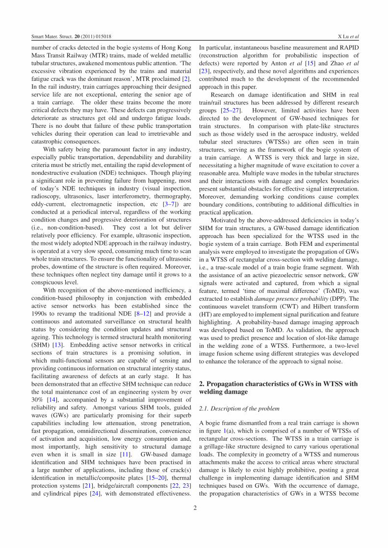
Figure 9. A typical raw signal from sensing path C4C5 in thepreparatory test.

boundaries of the WTSS, because the damage is located nearphysical edges of the WTSS. At the same time, different wavemodes existed in all captured signals. Though stimulated usingexcitations at carefully selected frequencies of 150, 175 and200 kHz so as to avoid interference from multiple modesin a GW signal, interaction of multiple wave modes wasunavoidable. Therefore, it is difficult to clearly distinguishdifferent wave components in captured GW signals. Thanks tothe relatively large magnitude, the dominant modes, the above-mentioned transverse modes, in signals could be isolated fromother signal components, like one example shown in figure 9.The two modes in this figure are wave components thattravelled directly from actuator to sensor and the minor one canbe recognized as a longitudinal mode that propagated faster.Through the preparatory test, the velocity of the dominant GWmode in the sample, Vd , was also calculated by dividing thedistance between actuator and sensor by the difference betweenthe arrival times of the excitation and dominant mode in thecorresponding sensing path, e.g. 276.6 mm and 90.5 μs forA1A3, and was determined as about 2950 m s−1 after averagingresults from multiple paths.

3.3. Experiment and signal processing

Experiments were conducted according to the configurationintroduced above. The same procedure was repeated withexcitations of different central frequencies. As observed inboth FE simulation (section 2.3) and experiment (section 3.2),captured GW signals in WTSSs are often complex inappearance, posing difficulty in damage identification. Aseries of signal processing was applied, including signal pre-processing (averaging), CWT and HT (please refer to [30]for detailed algorithms and expressions), with the aim ofde-noising and feature highlighting. For brief illustration,only raw and processed signals will be shown hereafter withderivations omitted. Furthermore, in order to avoid the extrainfluence of opposite-boundary reflections and circumferentialtransmission on signal interpretation, only the first fewcomponents of each GW signal were taken into account. Suchtruncation was applied to each collected signal, ensuring theabsence of those unwanted wave components.

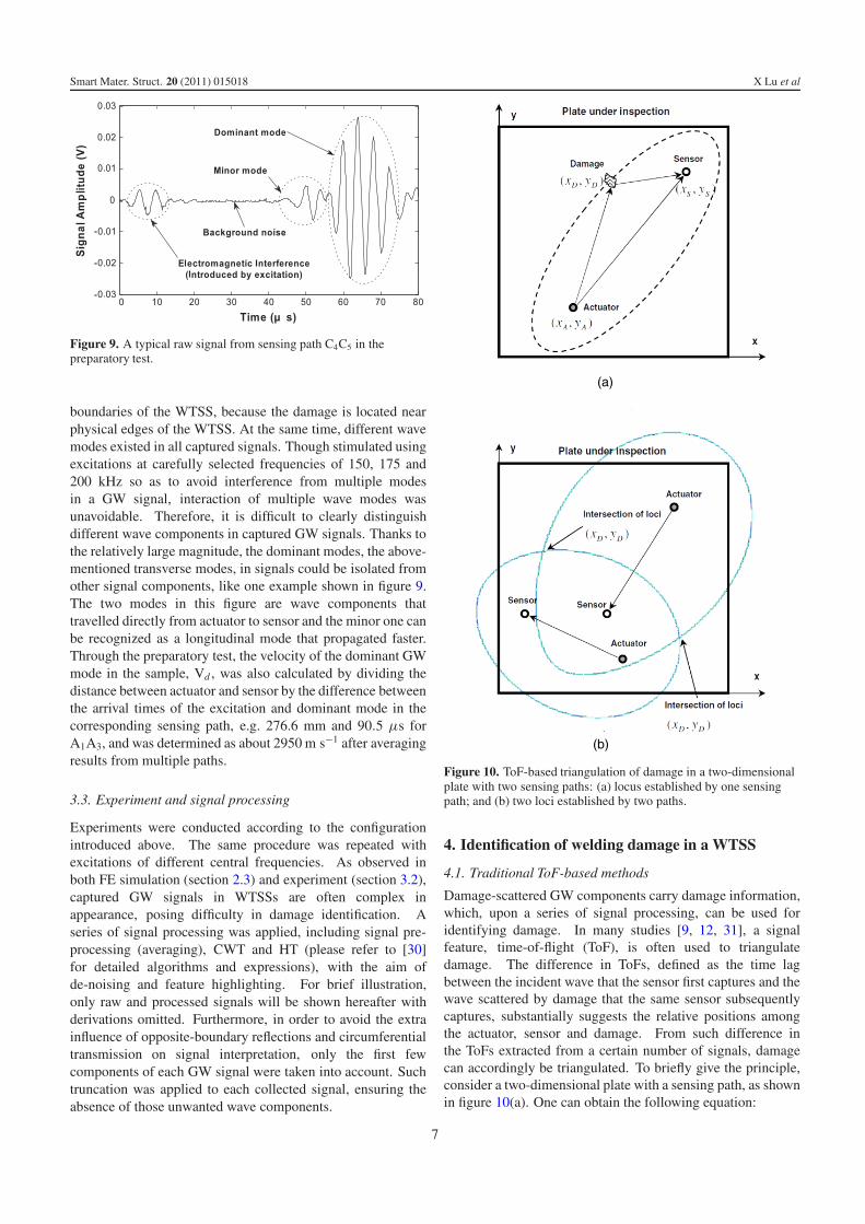
Figure 10. ToF-based triangulation of damage in a two-dimensionalplate with two sensing paths: (a) locus established by one sensingpath; and (b) two loci established by two paths.

4. Identification of welding damage in a WTSS

4.1. Traditional ToF-based methods

Damage-scattered GW components carry damage information,which, upon a series of signal processing, can be used foridentifying damage. In many studies [9, 12, 31], a signalfeature, time-of-flight (ToF), is often used to triangulatedamage. The difference in ToFs, defined as the time lagbetween the incident wave that the sensor first captures and thewave scattered by damage that the same sensor subsequentlycaptures, substantially suggests the relative positions amongthe actuator, sensor and damage. From such difference inthe ToFs extracted from a certain number of signals, damagecan accordingly be triangulated. To briefly give the principle,consider a two-dimensional plate with a sensing path, as shownin figure 10(a). One can obtain the following equation:

7

Smart Mater. Struct. 20 (2011) 015018 X Lu et al

Figure 11. Normalized signals for sensing path pair P2,3 under excitation at 150 kHz: (a) raw signals; (b) envelope of corresponding CWTcoefficients; and (c) envelope of the difference signal.

t = tA−D−S − tA−S =(

DA−D + DD−S

V

)− DA−S

V, (1)

whereDA−D =

√(xD − xA)2 + (yD − yA)2,

DD−S =√

(xS − xD)2 + (yS − yD)2,

DA−S =√

(xS − xA)2 + (yS − yA)2.

In the above equation, tA−D−S is the ToF of the incident wavepropagating from the actuator to the damage and then to thesensor, and tA−S is the ToF of the incident wave propagatingdirectly from the actuator to the sensor. t is the differencebetween the above two ToFs, which can be extracted fromthe captured GW signal. DA−D is the distance between theactuator located at (xA, yA), and the damage centre, presumedat (xD, yD) and to be determined; DD−S is the distance betweenthe damage centre and the sensor located at (xS, yS); DA−S isthe distance between the actuator and sensor. V is the groupvelocity of the incident GW activated by the actuator and theGW scattered by the damage. Theoretically, the solutions toequation (1) configure a locus, a dotted line in figure 10(a),indicating possible locations of the centre of the damage. WithToF extracted from another sensing path, an equation similar to

equation (1) can be obtained, and a nonlinear equation group,containing two equations contributed by two sensing pathsand involving the position of the damage centre (xD, yD) (twounknown variables), is available. Two loci established by thetwo equations lead to intersection(s), i.e., the solution(s) to theequation group, sketched in figure 10(b), which is (are) thelocation(s) of the damage centre (xD, yD).

However it is envisaged that, because of the complex su-perposition of various wave components in the WTSS men-tioned above and allowing for measurement noise/uncertaintiesunder demanding operational conditions, it is highly impos-sible to exactly locate damage based on the above-addressedprocedure.

4.2. ToMD and DPP-based damage imaging

In recognition of the fact that Facets A and C of the sample areentirely symmetrical regarding the symmetry plane as shownin figure 1(b) not only in geometry but also in active sensornetwork configuration, differences, if any, between capturedGW signals from corresponding sensing paths of two facetscan be fully attributed to the damage. For convenience ofdiscussion, Pm,n (m, n = 1, 2, . . . , 6, m = n) hereafter standsfor the arbitrary sensing path pair consisting of the sensing pathAmAn and its corresponding benchmark counterpart CmCn .

8

Smart Mater. Struct. 20 (2011) 015018 X Lu et al

Figure 12. ToMD-based determination of DPP on Facet A of theWTSS.

For a given Pm,n , two raw GW signals were captured (onevia CmCn and the other via AmAn). After applying averagingand CWT to raw signals, as described in section 3.3, HTwas subsequently employed to obtain the envelope of thedifference signal to highlight features of the signal in the timedomain, i.e., amplitude peaks and their corresponding arrivaltimes. In the envelope of the difference signal, the arrivaltime of local amplitude maximum was termed time of maximaldifference (ToMD) in regard to Pm,n , denoted by ToMDm,n

in what follows. Representatively, ToMDm,n extracted fromraw signals experimentally captured via P2,3 (i.e., ToMD2,3) isshown in figure 11.

Instead of exactly locating the damage, this studyfocused on determining damage presence probabilities (termedDPPs) at all locations on the WTSS. The following imagingalgorithm was developed to calculate DPP value(s) forarbitrary location(s) of the WTSS and firstly applied to Facet A.Without loss of generality, supposing that Facet A was meshedvirtually using K grids (e.g., 1×1 mm2 each in the following),the distance from a certain grid L j ( j = 1, 2, . . . , K ) to PZTwafer Am can be expressed as Dm, j = |rm

− r j| where rm

andr j are location vectors of Am and L j in the global coordinatesystem, as shown in figure 12. The time needed for GWs totravel along the route Am → L j → An can then be definedas Tm, j,n = (Dm, j + Dn, j )/Vd . Similar to equation (1) in the

above section, for the equation

ToMDm,n − Tm, j,n = 0, (2)

the coordinates of the damage centre are two unknownvariables. The solution of equation (2) presented an ellipselocus with the two PZT wafers being two foci, as portrayedwith a dash-dotted line in figure 12. In principle, the grids thatcorrectly locate on this locus, i.e., their coordinates can satisfyequation (2), have the highest probability of bearing damagefrom the prospect of the sensing path pair Pm,n that producessuch a locus. Therefore, the DPP values of these grids weredetermined as 100%.

For grids at other locations, their coordinates can neversatisfy equation (2). The further these grids are away from theellipse locus, the less the probability that they bear damage. Inthis sense, to quantify the DPP values at such grids in relationto their locations L j ( j = 1, 2, . . . , K ) and sensing path pairPm,n (m, n = 1, 2, . . . 6, m = n), a cumulative distributionfunction (CDF) [32] defined as

Fm,n(t) =∫ t

−∞f (T ′

m, j,n) dT ′m, j,n (3)

was then introduced where f (T ′m, j,n) = 1

σm,n√

2πexp[− (T ′

m, j,n)2

2σ 2m,n

]is the Gaussian distribution function, representing the densityfunction of the DPP. In the above equation, T ′

m, j,n =|ToMDm,n − Tm, j,n| is a function of L j when ToMDm,n isgiven, denoting the ‘distance’ between grid L j and the ellipselocus in time domain. σm,n is the standard variance and theintegral upper limit t is the value of T ′

m, j,n when m, j, n arespecified. Given a T ′

m, j,n , the DPP value of grid L j regardingPm,n becomes

DPP(L j , Pm,n) = 1 − |Fm,n(T ′m, j,n) − Fm,n(−T ′

m, j,n)| (4)

as exhibited in figure 13.Applying the above algorithm to all grids on Facet A,

an image for the estimated values of Pm,n involved DPP canbe obtained. After extending such a process to all otherfacets of the WTSS, a three-dimensional DPP image wasconstructed where damage was intuitionally visualized. As a

Figure 13. Gaussian distribution of the probability density in regard to the occurrence of damage at a specific grid of the WTSS.

9

Smart Mater. Struct. 20 (2011) 015018 X Lu et al

Figure 14. DPP image contributed by P2,4 (from experiment).

typical experimental result, the DPP image contributed by P2,4

is illustrated in figure 14. In this image, DPP values vary withinthe range of [0, 1] (indicated by grey-scale colours shown in thecolour bar) with the two extremes standing for the lowest andhighest DPP, i.e., 0% and 100%, respectively. Similar to someother recently developed imaging techniques for describing adamage event in engineered structures [23, 33–36], the darkerthe grey-scaled image appears, the greater the DPP of this gridis. Figure 14 suggested that the possible form of the damageis a large elliptical ring because all grids on the central line ofthe darkest region are of the same DPP value. In fact, damagecannot shape such a profile in real applications. The unrealisticestimation result indicated the insufficiency of determining thedamage location by information from a single sensing pathpair. Therefore, images contributed by all the available Pm,n

in the active sensor network were fused to configure out thecommon estimate of the damage location.

4.3. Two-level hybrid image fusion scheme

To strengthen the damage-associated information in the finalestimation result, a two-level hybrid image fusion scheme wasproposed based on conjunctive and compromised image fusiontechniques. For simplicity, DPP images established by all theavailable Pm,n were sorted according to the wave excitationfrequency (150, 175 and 200 kHz), denoted by Set-150k, Set-175k and Set-200k, respectively. Image fusion procedureswithin each image set and across sets, namely, the first andsecond level image fusions, were taken successively.

4.3.1. First level fusion. Taking Set-150k as an example,algebraic operations were applied to DPP values of allimages in Set-150k using conjunctive and compromised fusiontechniques which are respectively defined as

Conj DPP 150k(L j , P)

= NP

√√√√ m =n∏m,n∈1,2,...,6

DP P(L j , Pm,n),

j = 1, 2, . . . , K (5a)

Table 3. Set P: sensing path pairs involved in the first level imagefusion.

(A1A2, C1C2) (A3A1, C3C1) (A5A1, C5C1)(A1A3, C1C3) (A3A2, C3C2) (A5A2, C5C2)(A1A4, C1C4) (A3A4, C3C4) (A5A3, C5C3)(A1A5, C1C5) (A3A5, C3C5) (A5A4, C5C4)(A1A6, C1C6) (A3A6, C3C6) (A5A6, C5C6)(A2A1, C2C1) (A4A1, C4C1) (A6A1, C6C1)(A2A3, C2C3) (A4A2, C4C2) (A6A2, C6C2)(A2A4, C2C4) (A4A3, C4C3) (A6A3, C6C3)(A2A5, C2C5) (A4A5, C4C5) (A6A4, C6C4)(A2A6, C2C6) (A4A6, C4C6) (A6A5, C6C5)

Comp DPP 150k(L j , P)

= 1

NP

m =n∑m,n∈1,2,...,6

DP P(L j , Pm,n),

j = 1, 2, . . . , K (5b)

where P is the set of all involved sensing path pairs, as listedin table 3; NP is the number of elements in set P and is equalto 30 in this study. ‘Conj DPP 150k’ and ‘Comp DPP 150k’are so-called first level fusion results for Set-150k. Similarly,the same operation was applied to Set-175k and Set-200k.Figures 15 and 16 show the first level image fusion resultsfrom simulation and experiment data, respectively. DPP valuesin these fused images, as well as in the following ones, werenormalized in regard to the maximal DPP value of the currentimage, ensuring that the DPP values are always in the range [0,1].

In these two figures, dark areas representing estimatedwelding damage at the welding zone between Facets A andB are clearly observed. From all the subfigures we can seethat, referring to the real damage which is shown in contrastcolour, the estimated damage (the darkest area) in each imagecan more or less cover the real damage spot, indicating theeffectiveness of the recommended approach. Also, comparingfigure 15 with figure 16, an obvious similarity can befound, hinting that the predicted results from simulations andexperiments can match well. Moreover, although differentcolumns (representing different fusion techniques) in the samefigure offer predicted results in different views, the darkestareas maintain a relative constant location. As for theprecision of different fusion techniques and different excitationfrequencies, table 4 gives us a clear view and more details willbe addressed later in section 4.3.3.

4.3.2. Second level fusion. In order to enhance the accuracyof the estimate result by properly employing as much usefulinformation as possible, the second level image fusion, i.e.,fusion across DPP image sets for different excitations, wasundertaken. Both conjunctive and compromised schemeswere utilized again to combine the first level image fusionresults. By applying different strategies, four joint schemeswere established and are expressed below:

Comb DPP S1 = 3

√ ∏Freq∈150k,175k,200k

Conj DPP Freq (6a)

10

Smart Mater. Struct. 20 (2011) 015018 X Lu et al

Figure 15. Fused DPP images based on the first level image fusion (from simulation) for (a) Set-150k; (b) Set-175k; and (c) Set-200k usingconjunctive (left) and compromised (right) schemes.

Comb DPP S2 = 13

∑Freq∈150k,175k,200k

Conj DPP Freq (6b)

Comb DPP S3 = 3

√ ∏Freq∈150k,175k,200k

Comp DPP Freq (6c)

Comb DPP S4 = 13

∑Freq∈150k,175k,200k

Comp DPP Freq (6d)

where S1–S4 on the LHS stand for purely conjunctive,conjunctive–compromised, compromised–conjunctive, andpurely compromised schemes in turn. Figures 17 and 18 showthe results of the second level image fusion from simulation

11

Smart Mater. Struct. 20 (2011) 015018 X Lu et al

Figure 16. Fused DPP images based on the first level image fusion (from experiment) for (a) Set-150k; (b) Set-175k; and (c) Set-200k usingconjunctive (left) and compromised (right) schemes.

and experiment data, respectively. In the images, in spite of thecharacteristics similar to those in figures 15 and 16, approachof the estimated damage location to the real one, though notvery obvious due to the large dimensions of the WTSS, can befound, as detailed in section 4.3.3. Meanwhile, DPP imagesfor ‘Comb DPP S1’ and ‘Comb DPP S3’, as well as thosefor ‘Comb DPP S2’ and ‘Comb DPP S4’, can be found to be

highly accordant, implying the robustness of the second levelfusion.

4.3.3. Analysis of fusion results. Locations with the highestprobability of damage occurrence in figures 15–18 were pickedout and detailed in table 4. The coordinate system is thesame as that indicated in figure 1(b). The distances between

12

Smart Mater. Struct. 20 (2011) 015018 X Lu et al

Figure 17. Fused DPP images based on the second level image fusion (from simulation) using (a) purely conjunctive; (b)conjunctive–compromised; (c) compromised–conjunctive and (d) purely compromised schemes.

Table 4. Estimated damage locations from the two-level fusion procedure.

Estimated results from simulation Estimated results from experiment

CaseCoordinates(mm)

Distance toreal location(mm)

Relativeerror(%)

Coordinates(mm)

Distance toreal location(mm)

Relativeerror (%)

Real damage location (275, 0, 0) — — (275, 0, 0) — —

First level fusion Conj DPP 150k (276, 0,−8) 8.1 2.95 (282, 8, 0) 10.6 3.85Conj DPP 175k (291, 0,−1) 16.0 5.82 (270, 6, 0) 7.8 2.84Conj DPP 200k (281, 4, 0) 7.2 2.62 (253, 10, 0) 24.2 8.80Comp DPP 150k (275, 0,−7) 7.0 2.55 (282, 8, 0) 10.6 3.85Comp DPP 175k (291, 0,−1) 16.0 5.82 (281, 8, 0) 10.0 3.64Comp DPP 200k (281, 4, 0) 7.2 2.62 (260, 14, 0) 20.5 7.45

Second level fusion Comb DPP S1 (280, 0,−2) 5.4 1.96 (269, 6, 0) 8.5 3.09Comb DPP S2 (280, 0,−2) 5.4 1.96 (269, 6, 0) 8.5 3.09Comb DPP S3 (278, 0,−3) 4.2 1.53 (276, 7, 0) 7.1 2.58Comb DPP S4 (278, 0,−3) 4.2 1.53 (276, 7, 0) 7.1 2.58

estimated locations and the real damage position, as wellas relative errors which are ratios of these distances to thatbetween the real damage location and the origin, are alsoincluded in this table. It is found that: (1) comparing with thesample dimensions, the distances between estimated locationsand the real one are relatively small, implying the acceptabilityof the proposed approach; (2) whichever fusion schemes

were adopted in the two-level fusion procedure, obviousimprovement in identification accuracy can be observed whenthe second level fusion is applied, validating its necessity; and(3) although not every result of the second level fusion ismore accurate than those based on solely first level fusion, amore convincing decision can be drawn from the two-level datafusion procedure.

13

Smart Mater. Struct. 20 (2011) 015018 X Lu et al

Figure 18. Fused DPP images based on the second level image fusion (from experiment) using (a) purely conjunctive;(b) conjunctive–compromised; (c) compromised–conjunctive and (d) purely compromised schemes.

4.4. Analysis of error

The arithmetic of DPP stated in section 4.2 is sensitive toToMD. Any factor that can affect the ToMD value may leadto error in the DPP image derived from the single sensing pathpair. Such error could be amplified during the subsequentdata fusion procedure, especially under schemes containingconjunctive operation(s) [37]. In this study, many factorswould affect the final fusion results of the experiments. Firstly,uncertainties, such as the disparity in geometry betweenFacets A and C (despite the introduced damage), variationof welding quality, etc, are almost unavoidable. Secondly,weld ends, besides the induced damage, enlarge the expecteddamage zone so that the consequent fusion results would beaffected. Thirdly, the time duration of the wave componentof interest in the received signal is always longer than itsoriginal form due to the intrinsic dispersion characteristic ofthe GWs utilized. However, in virtue of the advantages of two-level data fusion, the errors from the different first level fusionresults are somewhat diminished. Taking all these matters intoconsideration, the fused results for damage location, as well astheir relative errors listed in table 4, are acceptable.

5. Conclusion

Propagation behaviour of GWs in a WTSS, a true-scalemodel of a train bogie frame segment containing slot-likewelding damage, was investigated in this study under thehypothesis that the WTSS is homogeneous. The damage-scattered wave components carrying damage information weremainly considered. An active sensor network consisting oftwelve PZT wafers was established to activate or collectGWs in the WTSS. Excitations at different frequencies wereused to obtain rich signals for investigation. An imagingapproach based on GW propagation and concepts, ToMDand DPP, was developed for estimation of damage presenceand location. A two-level image fusion scheme was furtherproposed with the aim of enhancing the robustness of theapproach to measurement noise and uncertainties. From theresults for estimation of damage location, it can be concludedthat, although the damage was located within the welding zoneand near the original edges of the WTSS, making damageevaluation much more difficult, acceptable estimation results ofdamage location can still be gained by applying the proposedimaging approach and the first level image fusion. Additionalimprovements in consistency and accuracy of the damageevaluation results were achieved when the second level fusion

14

Smart Mater. Struct. 20 (2011) 015018 X Lu et al

was performed. In brief, acceptable visualized evaluationof slot-like damage in the welding zone of a WTSS wasaccomplished using an approach combining GW propagationbased imaging and a two-level image fusion procedure,indicating the effectiveness of the recommended approach inevaluating presence and location of such welding damage inWTSSs and its large potential for real-time SHM of WTSSs.In addition, consideration of nonhomogeneity of the materialproperties and its potential impact on the characteristics ofwaves propagating in WTSSs will be addressed in future work.

Acknowledgments

The authors are grateful for the support received fromthe Research Grant Council of the Hong Kong SpecialAdministration Region (grant: PolyU5333/07E) and the HongKong Polytechnic University (grants: G-U204, 1-BBZN andA-PE1F).

References

[1] National Aeronautics and Space Administration (NASA) 2007Derailed Syst. Failure Case Stud. 1 1–4

[2] MTR Co. Ltd 2007 Circular for Rail Merger available from:http://www.mtr.com.hk/eng/investrelation/circulars2007/ew%200066cir%2020070903.pdf

[3] Achenbach J D 2000 Quantitative nondestructive evaluation Int.J. Solids Struct. 37 13–27

[4] Gray J and Tillack G-R 2001 X-ray imaging methods over thelast 25 years—new advances and capabilities Review ofProgress in Quantitative Nondestructive Evaluationvol 557A ed D O Thompson and D E Chimenti (New York:American Institute of Physics) pp 16–32

[5] Balageas D L 2002 Structural health monitoring R&D at the‘European Research Establishments in Aeronautics’ (EREA)Aerospace Sci. Technol. 6 159–70

[6] Sohn H, Farrar C R, Hemez F M, Shunk D D, Stinemates D Wand Nadler B R 2003 Review of structural health monitoringliterature: 1996–2001 Los Alamos National LaboratoryReport LA-13976-MS

[7] Boller C 2001 Ways and options for aircraft structural healthmanagement Smart Mater. Struct. 10 432–40

[8] Alleyne D N and Cawley P 1992 The interaction of Lambwaves with defects IEEE Trans. Ultrason. Ferroelectr. Freq.Control 39 381–97

[9] Kessler S S, Spearing S M and Soutis C 2002 Damagedetection in composite materials using Lamb wave methodsSmart Mater. Struct. 11 269–78

[10] Staszewski W J, Boller C and Tomlinson G R 2004 HealthMonitoring of Aerospace Structures: Smart SensorTechnologies and Signal Processing (New York: Wiley)

[11] Raghavan A and Cesnik C E S 2007 Review of guided-wavestructural health monitoring Shock Vib. Dig. 39 91–114

[12] Giurgiutiu V and Bao J 2004 Embedded-ultrasonics structuralradar for in situ structural health monitoring of thin-wallstructures Struct. Health Monit. 3 121–40

[13] Moyo P and Brownjohn J M W 2002 Detection of anomalousstructural behaviour using wavelet analysis Mech. Syst.Signal Process. 16 429–45

[14] Chang F K 2002 Introduction to health monitoring: context,problems, solutions Presentation at the 1st EuropeanPre-workshop on Structural Health Monitoring (Paris, July2002)

[15] Anton S R, Inman D J and Park G 2009 Reference-free damagedetection using instantaneous baseline measurements AIAAJ. 47 1952–64

[16] Badcock R A and Birt E A 2000 The use of 0–3 piezocompositeembedded Lamb wave sensors for detection of damage inadvanced fibre composites Smart Mater. Struct. 9 291–7

[17] Lin X and Yuan F G 2005 Experimental study applying amigration technique in structural health monitoring Struct.Health Monit.—Int. J. 4 341–53

[18] Ostachowicz W, Kudela P, Malinowski P andWandowski T 2009 Damage localisation in plate-likestructures based on PZT sensors Mech. Syst. Signal Process.23 1805–29

[19] Park H W, Sohn H, Law K H and Farrar C R 2007 Timereversal active sensing for health monitoring of a compositeplate J. Sound Vib. 302 50–66

[20] Ihn J B and Chang F K 2004 Detection and monitoring ofhidden fatigue crack growth using a built-in piezoelectricsensor/actuator network: I. Diagnostics Smart Mater. Struct.13 609–20

[21] Kundu T, Das S and Jata K V 2009 Health monitoring of athermal protection system using lamb waves Struct. HealthMonitor.—Int. J. 8 29–45

[22] Park S, Yun C-B, Roh Y and Lee J-J 2006 PZT-based activedamage detection techniques for steel bridge componentsSmart Mater. Struct. 15 957–66

[23] Zhao X L, Gao H D, Zhang G F, Ayhan B, Yan F, Kwan C andRose J L 2007 Active health monitoring of an aircraft wingwith embedded piezoelectric sensor/actuator network: I.Defect detection, localization and growth monitoring SmartMater. Struct. 16 1208–17

[24] Tua P S, Quek S T and Wang Q 2005 Detection of cracks incylindrical pipes and plates using piezo-actuated Lambwaves Smart Mater. Struct. 14 1325–42

[25] Barke D and Chiu W K 2005 Structural health monitoring in therailway industry: a review Struct. Health Monitor. 4 81–93

[26] Rose J L, Avioli M J and Song W-J 2002 Application andpotential of guided wave rail inspection Insight 44 353–8

[27] Wilcox P, Evans M, Pavlakovic B, Alleyne D N, Vine K,Cawley P and Lowe M 2003 Guided wave testing of railInsight 45 413–20

[28] Rose J L 1999 Ultrasonic Waves in Solids (New York:Cambridge University Press)

[29] Su Z and Ye L 2004 Selective generation of Lamb wave modesand their propagation characteristics in defective compositelaminates Proc. Inst. Mech. Eng. L 218 95–110

[30] Su Z Q and Ye L 2009 Identification of Damage Using LambWaves: From Fundamentals to Applications (London:Springer)

[31] Lu Y, Ye L, Su Z Q and Yang C H 2008 Quantitativeassessment of through-thickness crack size based on Lambwave scattering in aluminium plates NDT&E Int. 41 59–68

[32] Walpole R E, Myers R H and Myers S L 1998 Probability andStatistics for Engineers and Scientists (Upper Saddle River,NJ: Prentice-Hall)

[33] Ihn J B and Chang F K 2008 Pitch-catch active sensingmethods in structural health monitoring for aircraftstructures Struct. Health Monit.—Int. J. 7 5–19

[34] Wang C H, Rose J T and Chang F K 2004 A synthetictime-reversal imaging method for structural healthmonitoring Smart Mater. Struct. 13 415–23

[35] Michaels J E and Michaels T E 2007 Guided wave signalprocessing and image fusion for in situ damage localizationin plates Wave Motion 44 482–92

[36] Konstantinidis G, Wilcox P D and Drinkwater B W 2007 Aninvestigation into the temperature stability of a guided wavestructural health monitoring system using permanentlyattached sensors IEEE Sensors J. 7 905–12

[37] Su Z Q, Wang X M, Cheng L, Yu L and Chen Z P 2009 Onselection of data fusion schemes for structural damageevaluation Struct. Health Monit. 8 223–41

15