evaluation of the wind field distribution in the rossby .../internship_report_daniel... ·...
TRANSCRIPT
Rossby Centre, SMHI∗ & Wageningen University+
Internship Report Meteorology & Air Quality
Evaluation of the Wind Field Distribution in theRossby Centre Regional Climate Model RCA4 over
the North Sea for 1979-2010
Author:B. D. J. Kunne
Supervisors:C. G. Jones∗
S. Wang∗
P. Samuelsson∗
W. Hazeleger+
L. J. M. Kroon+
August 2, 2012
Abstract
Near-surface wind modelling yields a variety of possibilities in the field of wind energy and futureclimate variability. In this study, the newly developed RCA4 model from the SMHI is evaluatedagainst observations from a set of eleven stations over the North Sea. For this analysis, threeseparate runs (i.e. RCASA, HICOR and LOCOR) with different horizontal resolutions and alteredCharnock constants are compared over the period from 1979 to 2010. In the central-northernregion, all three runs consistently overestimate the actual 10m wind speed, while the RCASArun is able to reproduce the observations more accurately in the southern part of the North Sea.Evaluation of the trend in RCA4 reveals that the model yields a high temporal cross-correlationwith the measurements, while the 10m wind direction is consistently overestimated in the model,much of which is linked to the ageostrophic component of the wind. The statistical properties of thewind field are analysed with the use of a probability density function (PDF) and the relationshipbetween the normalized wind speed and the skewness of the distribution. Especially the HICORand LOCOR run show a pronounced deviation from the observations in terms of this latter relation,suggesting that the nature of the PDF is significantly different. The mean of the high-speed endof the PDF is typically overestimated in RCA4, though the variance of the upper 90th percentileis widely underestimated with respect to actual measurements. Separation of the data into threeregimes, based on the static stability conditions, lead to the conclusion that LOCOR overestimatesthe wind speed PDF under unstable conditions, possibly due to its lower resolution. Comparisonof the relation between the sea level pressure and the M10, however, showed that the LOCOR isthe better of the three runs in all regimes. In the RCASA and HICOR run, similar differences ariseunder both stable and unstable conditions, which are most likely to be related to the turbulentkinetic energy budget, and the respective production and destruction of turbulence by wind shearand buoyancy.

Contents
1 Introduction 2
2 Data Description 4
3 Near-Surface Wind Field 73.1 Wind Speed Time Series . . . . . . . . . . . . . . . . . . . . . . . . . . . . . . . . . . 73.2 Cross-Correlations . . . . . . . . . . . . . . . . . . . . . . . . . . . . . . . . . . . . . 93.3 Wind Direction . . . . . . . . . . . . . . . . . . . . . . . . . . . . . . . . . . . . . . . 10
4 Statistical Characteristics 144.1 Probability Density Functions . . . . . . . . . . . . . . . . . . . . . . . . . . . . . . . 144.2 Statistical Relationships & Extremes . . . . . . . . . . . . . . . . . . . . . . . . . . . 16
5 Stability Conditions 205.1 Stability Regimes . . . . . . . . . . . . . . . . . . . . . . . . . . . . . . . . . . . . . . 205.2 Sea Level Pressure Field . . . . . . . . . . . . . . . . . . . . . . . . . . . . . . . . . . 22
6 Discussion & Recommendations 26
A Model Coordinates 30
B PDF Statistical Tables 31
C NCL Scripts 33
D Self Reflection 38
E About SMHI 41
1

Chapter 1
Introduction
While the energy market is on the transition from convential energy (e.g. coal and oil) towardsrenewable energy (e.g. wind and hydropower), knowledge of the near-surface wind field gains con-siderable interest. For many applications in the field of wind energy, extreme weather forecastingand surface flux estimations, knowledge of the wind field characteristics is important (Petersen etal., 1998a,b; Jagger et al., 2001; Monahan, 2006a). Since the potential for wind energy over seasis greater than for most terrestrial locations (US Dept. of Energy, 2012), focus shifts to offshoreregions. Knowledge of the wind field in the marine atmospheric boundary layer is important, sincearound 70% of the Earth’s surface is covered by water. Our daily lifes are affected by the manyprocesses occuring in the atmosphere over the oceans (Pena et al., 2008). Regional models canbe used to select suitable sites for offshore wind farms and provide us with an outlook for futureclimate variability. Drawback of offshore wind field evaluation is the lack of reliable and consistentobservations over seas, which can act as a reference for the quality of model results. Only fewdata series from oil platforms, light ships and wind farms are available, leaving extensive areaswithout data. To overcome this issue, one needs to ensure itself of the accuracy of the used modelover locations where data is available. If done so, this model can be applied to the gap areas as well.
At the Rossby Centre of the SMHI in Norrkoping, Sweden, the Rossby Centre Regional ClimateModel (RCA) is continuously adjusted and improved. Since RCA3 (Samuelsson et al., 2010), RCAhas undergone both physical and technical changes (Kupiainen et al., 2011). Recently, the newestversion, RCA4, has been developed. He et al. (2010) have analyzed the 10m wind speed climatein RCA3 thoroughly, against a large dataset of synoptic weather reports over North America. Al-though RCA3 has shown to perform generally better than other regional climate models (RCM’s),they noted that the median wind speeds are underestimated. For water-dominated regions, the highwind-speed end of the distribution is underestimated as well. Near-surface wind speeds are verysensitive to the horizontal resolution of regional models. An increased resolution of RCA in newerversions of the model, therefore, offers a high potential for representing the wind field distributionand the occurence of more extreme events over open water more accurately. Analysis, similar tothat of He et al. (2010) and Monahan et al. (2011), will reveal whether improvements are made insimulating the near-surface wind field in RCA4.
2

CHAPTER 1. INTRODUCTION 3
With the preliminary results of the RCA model, as mentioned, taken into account, the researchquestions set for this study are:
- Is the RCA4 model able to yield an accurate representation of the temporal and statisticalcharacteristics of the wind field at set locations over the North Sea?
- What are the effects of adjusted wind stress and stability conditions in an ensemble of modelruns, and how do they compare against reanalysis data and observations?
- What are the major offsets of the RCA4 model and what parameters deserve greatest atten-tion from a modeling perspective? Essentially, how can we improve on the model in its presentstate?
This study aims to qualify the performance and possibilities of RCA4 over the North Sea. Inthe Data Description section of this report, the details of the RCA4 model and its specific runsused in this study are stated. Furthermore, an overview of the locations where observational datais gathered, both at oil platforms and aboard light ships, is given. Hereafter, statistical and tem-poral analysis is used to compare model results with reanalysis data and actual measurements inChapters 3 and 4. A variety of statistical tools are applied, amongst which the temporal cross-correlation and the probability density function (PDF). Essentially, challenges for offshore windresource assessment come from the dependence on surface roughness as well as stability (Landberget al., 2003). Therefore, the consistency of several model runs during different seasons and stabilityregimes is analyzed in Chapter 5 to improve the understanding of the model’s behaviour undervarying circumstances. Finally, the most important results are discussed and recommendations forfurther study and regional climate modelling are given.
Chapter 2
Data Description
Throughout the last decades, oil platforms and rigs have been built over the North Sea. For bothcommercial and scientific purposes those platforms are often equipped with meteorological equip-ment, such as anemometers and barometers. This set-up allows for multi-year time series of thewind and pressure field on locations where consistent data series are scarce. Moreover, light shipshave been measuring synoptic conditions in coastal regions. Retrieval of platform and light shipdata is troublesome, since not all data is freely available and there is no all-including data archivefor open water time series yet. Nevertheless, by combining measurements from five different sources,we have been able to select proper time series for a total of eleven stations, spread out over the fulllatitudinal range of the North Sea. Table 2.1 summarizes the specifications of each station. KNMIprovided us with long time series from the Europlatform and K13 platform, as part of the HydraProject (KNMI, 2011). Both are oil platforms, as are the three locations in the Norwegian part ofthe North Sea, provided by Magnar Reistad, from the Norwegian Meteorolgisk Institutt (MetNo).The Frigg oil field is also located in Norwegian waters, but data for this station has been obtainedfrom a dataset by Dai & Deser (1999), offered to us by Yanping He. With this huge dataset, wehave found data for two British platforms as well, i.e. Auk and North Cormorant. Tinz Bergerfrom the Deutsche Wetterdienst (DWD) provided us with early data from two light ships, namelythe Elbe 1 and the Deutsche Bucht. In the same region a brand new wind farm has been developed,FINO 1, which includes wind speed data from 2004 onwards (DEWI, 2008).
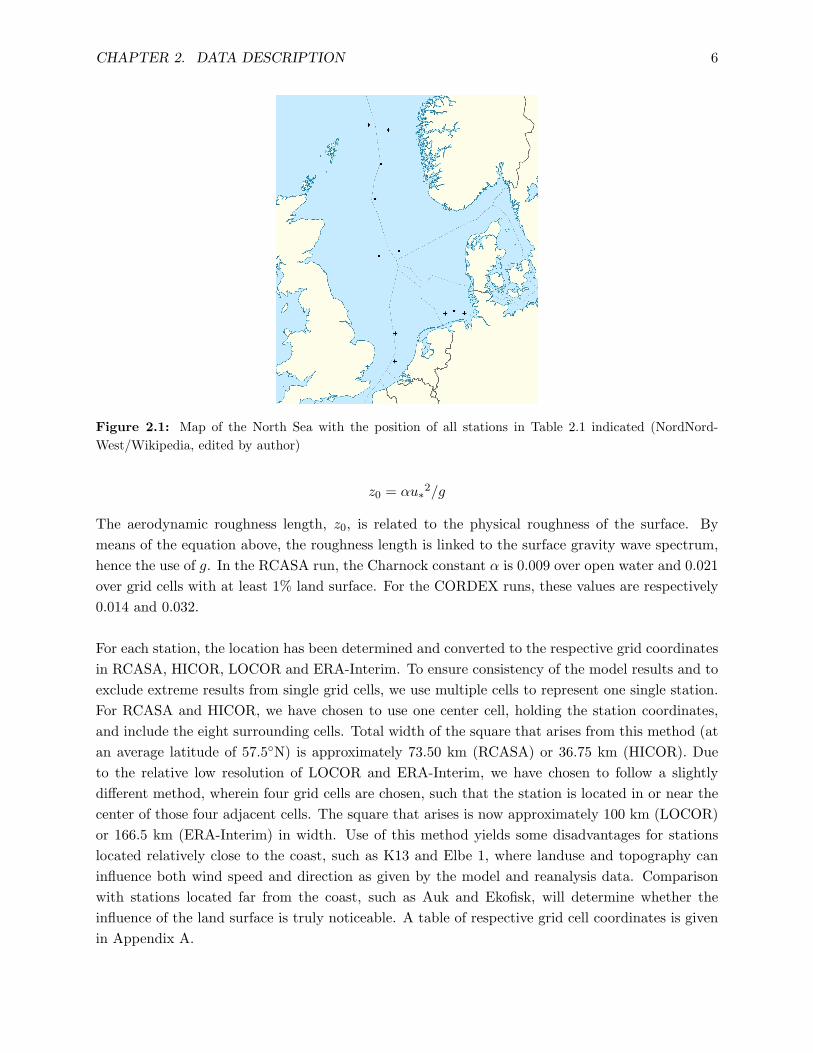
The position of all eleven stations is indicated in Figure 2.1, which shows that we include most ofthe North Sea regions in our analysis, except for the Danish waters. Near-coastal stations (<30 kmfrom the coast) have been left out of this selection, to assure we are in any case focussing on theopen-water conditions, rather than incorporating too much of the effect of land in coastal regions.As can be seen from Table 2.1, the majority of the stations does not cover the entire time periodfrom 1979 up to 2010. Many of the platforms were built throughout this period, and therefore datais only avaible from a later time. The stations are chosen such, that they all provide us with atleast seven years of consistent data on a set location. Since the height at which the wind speedand direction are measured ranges from 18 meters above the sea surface at both light ships upto approximately 100 meters at some of the oil platforms, we chose to convert all winds to the
4

CHAPTER 2. DATA DESCRIPTION 5
10 meter wind speed (M10). If not already done by the respective source, this has been done bymeans of a wind profile power law, where the exponent α is set to 0.11, corresponding to neutralstability conditions over open water. Furthermore, negative wind speeds have been omitted andset to missing values in the data. Whenever the data showed very irregular measurements withgaps of several weeks or months, the specific period is entirely omitted from the dataset as well.No further adjustments have been done to the raw observation data.
Table 2.1: Specifications Observations and Model Runs
Name Longitude (◦E) Latitude (◦N) Meas. height (m) Period Source
Europlatform 03.28 51.99 29.1 1983-2005 KNMIK13 03.22 53.22 73.8 1983-2004 KNMI
Ekofisk 03.20 56.50 70.2 1980-2010 MetNoSleipner 01.90 58.40 70 - 110 1995-2010 MetNoGullfaks 02.30 61.20 70 - 110 1990-2010 MetNo
Frigg 02.00 59.93 95.0 1988-2005 DaiAuk 02.07 56.40 34.0 1988-2005 Dai
North Cormorant 01.15 61.23 47.0 1988-2005 DaiDeutsche Bucht 07.26 54.11 18.0 1979-1986 DWD
Elbe 1 08.07 54.00 18.0 1979-1988 DWDFINO 1 06.58 54.02 33.0 2004-2010 BMU/PTJ
Name Hor. resolution (◦) Temp. resolution (hr) Period Source
RCASA 0.22 3-6 1979-2010 SMHIHICOR 0.11 3-6 1979-2010 SMHILOCOR 0.44 3-6 1980-2010 SMHI
ERA-Interim 0.75 6 1979-2010 ECMWF
Our primary run is the RCASA on a stand-alone basis over the North Sea region. This runs on a hor-izontal resolution of 0.22◦ on a rotated latitude-longitude grid with 40 vertical levels (Wang, 2012).It covers the period of 1979 to 2010 and it is initialized and driven by ECMWF’s ERA-Interimreanalysis data. Therefore, the ERA-Interim (on a 0.75◦ resolution) is included as a reference. Inaddition to this model run, two runs of the Coordinated Regional Climate Downscaling Experiment(CORDEX) are included in the analysis. The CORDEX model runs with the same specifics as theRCASA, except for its horizontal resolution. The HICOR runs on a high resolution of 0.11◦, whilethe LOCOR runs on a relatively low resolution of 0.44◦. Furthermore, the Charnock constant hasbeen adjusted to match the wind stress conditions over sea surfaces. The Charnock (1955) relationis given by:
CHAPTER 2. DATA DESCRIPTION 6
Figure 2.1: Map of the North Sea with the position of all stations in Table 2.1 indicated (NordNord-West/Wikipedia, edited by author)
z0 = αu∗2/g
The aerodynamic roughness length, z0, is related to the physical roughness of the surface. Bymeans of the equation above, the roughness length is linked to the surface gravity wave spectrum,hence the use of g. In the RCASA run, the Charnock constant α is 0.009 over open water and 0.021over grid cells with at least 1% land surface. For the CORDEX runs, these values are respectively0.014 and 0.032.
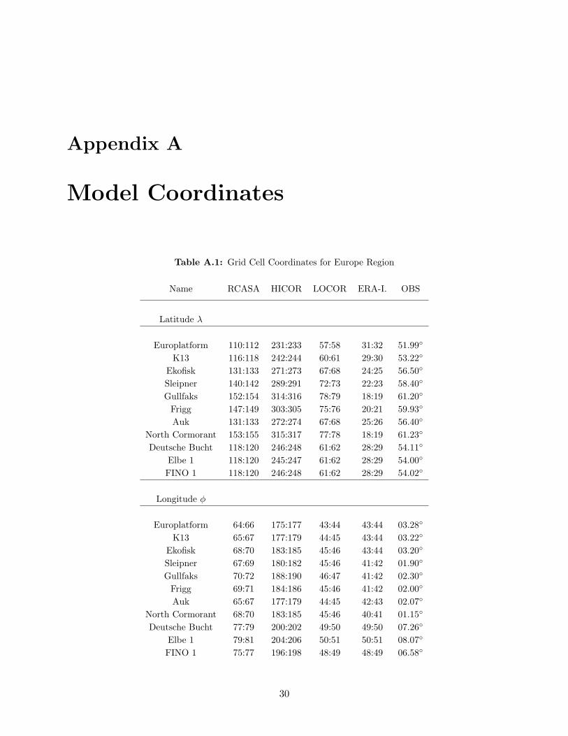
For each station, the location has been determined and converted to the respective grid coordinatesin RCASA, HICOR, LOCOR and ERA-Interim. To ensure consistency of the model results and toexclude extreme results from single grid cells, we use multiple cells to represent one single station.For RCASA and HICOR, we have chosen to use one center cell, holding the station coordinates,and include the eight surrounding cells. Total width of the square that arises from this method (atan average latitude of 57.5◦N) is approximately 73.50 km (RCASA) or 36.75 km (HICOR). Dueto the relative low resolution of LOCOR and ERA-Interim, we have chosen to follow a slightlydifferent method, wherein four grid cells are chosen, such that the station is located in or near thecenter of those four adjacent cells. The square that arises is now approximately 100 km (LOCOR)or 166.5 km (ERA-Interim) in width. Use of this method yields some disadvantages for stationslocated relatively close to the coast, such as K13 and Elbe 1, where landuse and topography caninfluence both wind speed and direction as given by the model and reanalysis data. Comparisonwith stations located far from the coast, such as Auk and Ekofisk, will determine whether theinfluence of the land surface is truly noticeable. A table of respective grid cell coordinates is givenin Appendix A.
Chapter 3
Near-Surface Wind Field
Evaluation of the near-surface wind field in the RCA4 model contributes to the physical under-standing of the model’s strengths and weaknesses. This chapter introduces the 10m wind speedtime series from the observations and shows the results of a first, basic comparison with the modeland reanalysis data.
3.1 Wind Speed Time Series
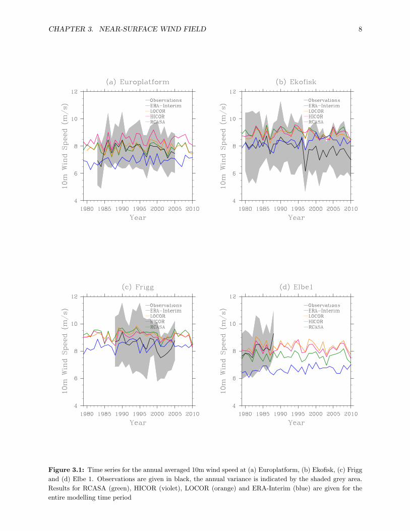
A straightforward method to reveal some of the wind field characteristics in both observationsand models is a time series of the temporally averaged wind speed. For each station, the annualaveraged 10m wind speed (M10) has been determined. Results are shown for four of the stations(i.e. Europlatform, Ekofisk, Frigg and Elbe 1) in Figure 3.1, covering all present regions of theNorth Sea and almost all data sources (see Table 2.1). The remaining stations are taken into con-sideration, but are not shown for graphical convenience. The observations are given in black andthe annual variance is indicated by the shaded grey area. The model runs and reanalysis data arerepresented by the coloured lines (see legend for colour definition). The results for the observationsare restricted to the time period covered by the actual measurements. The models, however, ranover the full time period from 1979 up to 2010. This enhances the possibilities to intercompare theindividual model runs over a longer period and look for a systematic bias between the runs.
The five stations near the German and Dutch coast, covering the southern part of the North Sea,show great similarities. Due to the relatively low horizontal resolution in the LOCOR run, we wereforced to select the ocean-only tiles, to avoid land surface friction effects in coastal areas, whichcause the wind speed close to the surface to be significantly lower than for ocean-only conditions.After this adjustment, HICOR and LOCOR yield approximately the same results for four out offive stations. Europlatform is the exception, at which the LOCOR run has consistently lower val-ues than the HICOR run throughout the full extent of the time series. The RCASA run showssomewhat different results, with very consistently lower values at all five stations in this region.This seems a bit counter-intuitive, since the smaller Charnock constant in RCASA implies lessdrag from the surface and consequently higher wind speeds closer to the surface, compared to both
7
CHAPTER 3. NEAR-SURFACE WIND FIELD 8
Figure 3.1: Time series for the annual averaged 10m wind speed at (a) Europlatform, (b) Ekofisk, (c) Friggand (d) Elbe 1. Observations are given in black, the annual variance is indicated by the shaded grey area.Results for RCASA (green), HICOR (violet), LOCOR (orange) and ERA-Interim (blue) are given for theentire modelling time period

CHAPTER 3. NEAR-SURFACE WIND FIELD 9
CORDEX runs. This raises the question whether the decrease in the Charnock constant is notsufficient to yield any increase in the wind speeds or whether another effect is overcompensatingthis Charnock effect. More on the subject will de discussed in Chapter 5 on the wind field behaviourunder different stability conditions. For now, it is promising to see that especially the RCASA runis well able to approximate the trend and value of the measurements in this region of the North Sea.
The central and northern part of the North Sea, covered by the remaining six stations, showsa similar relation between the HICOR and LOCOR run. Results for both CORDEX runs ex-perience a consistent overestimation of the observations. In contrast to the southern region, theRCASA now also shows a distinct positive bias compared to the observations. Results for theRCASA are close to those for CORDEX in terms of both annual averaged values and multi-yeartrends. ERA-Interim, significantly underestimating the observations in the sourthern part of theNorth Sea, shows reasonable correspondence with the observed M10 in the other regions. Themulti-year trend is, however, very different from what the observations indicate. In general, we canargue that the RCASA run is very well able to represent the trend, as observed at all stations, butyields a clear overestimation for at least half of the stations considered. Both HICOR and LOCORdo not show any clear improvements on these results and are consequently outperformed by theformer model run.
3.2 Cross-Correlations
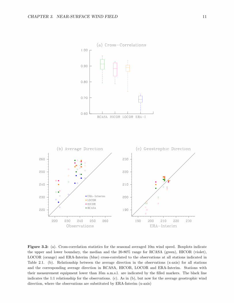
By evaluating the statistical correspondence, in terms of the so-called cross-correlation, one ne-glects the presence of any positive or negative bias and one focuses solely on the difference in thetrend or evolution. We have calculated the seasonal averaged M10 at all stations and determinedthe cross-correlation between the observations and all model runs and the ERA-Interim data. Thecorresponding values are given in Table 3.1. A value of 1 indicates a perfect match, while a valueof 0 indicates that there is no correlation between the two time series whatsoever. In order tovisualize these results, Figure 3.2 shows the spread of the cross-correlations by means of a boxplot,showing the median, the upper and lower boundary and the 20-80% range for all model runs.
As we already noted in the previous section, the trend correlation in ERA-Interim is lowest of allsimulations, with an average cross-correlation of a mere 0.68. Except for the FINO 1 wind energypark, the stations show very similar results and the spread of the results is relatively low, comparedto the three model runs. However, much of this enhanced spread in the models is caused by onesingle station, the North Cormorant. Surprisingly enough, it is that particular station showingthe largest cross-correlation in ERA-Interim, while it clearly shows the weakest correspondence inRCASA and CORDEX. Reason for this striking difference is presumably the irregularity in theobservations. Periods of weeks or months with no or insufficient measurements occured multipletimes throughout the whole time period. These gaps in the data will disturb the derived evolutionof the annual average and do eventually affect the reliability of the measurements at this specificlocation.

CHAPTER 3. NEAR-SURFACE WIND FIELD 10
Table 3.1: Cross-Correlations of the Seasonal M10
Name RCASA vs. OBS HICOR vs. OBS LOCOR vs. OBS ERA-I. vs. OBS
Europlatform 0.91880 0.88317 0.88371 0.71191K13 0.86829 0.82891 0.82547 0.69149
Ekofisk 0.88034 0.84005 0.86566 0.68442Sleipner 0.94234 0.92631 0.90495 0.67102Gullfaks 0.96474 0.92826 0.92469 0.71869
Frigg 0.94795 0.92058 0.90412 0.69197Auk 0.89627 0.86960 0.86994 0.67616
North Cormorant 0.79230 0.78803 0.73812 0.72397Deutsche Bucht 0.91270 0.88721 0.89165 0.68932
Elbe 1 0.93565 0.91258 0.93565 0.67719FINO 1 0.90368 0.83707 0.90042 0.62151
The resemblance of RCASA with the observations is very promising. Although the model is drivenby ERA-Interim, it is well able to improve on the reanalysis data results. It also outperforms bothCORDEX runs at every station, albeit by a much smaller difference. Strikingly enough, the lower-resolution LOCOR run shows slightly higher cross-correlations, mainly in the southern part of theNorth Sea, compared to its higher-resolution counterpart, HICOR. It seems as if the benificial effectof a more detailed description of the M10 is either negligible or entirely compensated by anothermechanism, only present in the HICOR model run. Possibly, the wind stress coefficient, representedby the Charnock constant, has a much more pronounced effect on smaller scale atmospheric systemsand therefore expresses itself more clearly in the high-resolution results. Nonetheless, differencesbetween the three model runs are relatively small and one could argue that both the RCASA runand the CORDEX runs correspond well with the observations.
3.3 Wind Direction
The near-surface wind field is characterized by its velocity, as depicted in the previous sections,and by its direction. Accurate modelling of the wind direction is key, since it determines the originof the winds over a certain area. Air from the European mainland is significantly different thanair from the Norwegian Sea, in terms of e.g. temperature and humidity. In a practical sense, theprediction of wind direction is necessary for the intelligent placement and efficient operation of windenergy turbines (Hirata et al., 2008). Therefore, we derived the wind direction distributions at allstations and calculated the average 10m wind direction for all model runs. Since the average winddirection is strongly dependent on the location rather than on the data source, we split the elevenstations into five regions. This way, stations from different sources are combined and we reduce theerror margins caused by a single source. Especially in the German region, it is benificial to use theFINO1 wind energy field data at a much later point in time (2004-2010) as a counterpart to the two
CHAPTER 3. NEAR-SURFACE WIND FIELD 11
Figure 3.2: (a). Cross-correlation statistics for the seasonal averaged 10m wind speed. Boxplots indicatethe upper and lower boundary, the median and the 20-80% range for RCASA (green), HICOR (violet),LOCOR (orange) and ERA-Interim (blue) cross-correlated to the observations at all stations indicated inTable 2.1. (b). Relationship between the average direction in the observations (x-axis) for all stationsand the corresponding average direction in RCASA, HICOR, LOCOR and ERA-Interim. Stations withtheir measurement equipment lower than 35m a.m.s.l. are indicated by the filled markers. The black lineindicates the 1:1 relationship for the observations. (c). As in (b), but now for the average geostrophic winddirection, where the observations are substituted by ERA-Interim (x-axis)

CHAPTER 3. NEAR-SURFACE WIND FIELD 12
light ships Deutsche Bucht (1979-1986) and Elbe 1 (1979-1988). The stations are divided as follows:
I. Netherlands: Europlatform & K13II. Centre: Ekofisk & AukIII. Norway: Sleipner & FriggIV. North: Gullfaks & North CormorantV. Germany: Elbe 1 & Deutsche Bucht & FINO 1
Table 3.2 shows the results for all five regions and the average of those results. In the previous sec-tion we noted that the RCASA was very well able to represent the actual wind speed and that bothCORDEX runs performed slightly less good. For the wind direction, both HICOR and LOCORperform significantly less than the RCASA run. While the RCASA shows a clear overestimationof the north-westerly component of the actual wind in all regions of about 11 to 12 degrees, theHICOR run yields an even greater overestimation of 17 to 18 degrees. The LOCOR shows a slightlysmaller bias of approximately 16 degrees, which still accounts for a decent shift in the average windfield. Why the HICOR is apparently unable to improve on the results of the LOCOR run is ques-tionable, since it is ought to be better in representing both the larger synoptic and smaller-scaleatmospheric systems more truthfully and therefore yield a better correspondence with the actualwind direction. Although the ERA-Interim reanalysis performed relatively weak in modeling theM10, its performance in terms of wind direction is much better and it outperforms the simulationruns, with an average overestimation of about 3 to 4 degrees. To verify that the overestimations ascalculated are indeed approximately constant over the extent of the North Sea, we have includedthe one on one relationship of the observations with the results for the four simulations in Figure3.2b. In this figure, the stations with their measurement equipment lower than 35 meters above thesurface are indicated by the filled markers, in contrast to those higher than 35 meters, indicated bythe unfilled markers. This is done to verify that the original height has no noticeable influence andall stations are suitable for further analysis, although converting wind speeds from higher up in theboundary layer towards the surface does not include any directional shift or ekman spiralling.
The wind direction basically consists of a geostrophic and an ageostrophic part, where the geostrophicwind direction is determined by the surface pressure gradient and the Coriolis force at the respectivestation locations. The measurements lack information on the sea level pressure (SLP). However,since the general direction is reasonably well presented in ERA-Interim and the reanalysis data isought to be a good representation of the actual pressure field, we use ERA-Interim as a reference.Results for the geostrophic wind direction are shown in Figure 3.2c. Differences between the ERA-Interim and the model runs are much smaller than for the general direction and yield both over- andunderestimations of the reanalysis data, in the central-northern and southern region, respectively.Averaged over the entire North Sea, differences range from 0.09 (LOCOR) to -0.73 (RCASA) and-0.82 (HICOR). It is therefore safe to argue, that much of the directional inconsistencies of themodels appear in the ageostrophic, rather than the geostrophic component of the wind. Errors inthe representation of the intensity, extent and path of low- and high-pressure systems over the re-

CHAPTER 3. NEAR-SURFACE WIND FIELD 13
Table 3.2: Average Direction Statistics
Region RCASA HICOR LOCOR ERA-I. OBS
Netherlands 250.5 256.0 255.0 246.0 240.5Centre 250.0 258.5 254.5 243.0 239.0Norway 238.0 247.5 244.5 230.0 227.5North 232.5 239.0 237.5 224.0 223.0
Germany 256.7 254.7 257.0 244.7 238.3
Avg. difference RCASA - OBS HICOR - OBS LOCOR - OBS ERA-I. - OBS
All Regions 11.88 17.48 16.04 3.88
gion are presumably of major influence in this respect. This is, however, not completely satisfying,since a higher horizontal resolution in the HICOR run is supposed to yield a better respresentationof those systems. More thorough evaluation of the influence of smaller-scale atmospheric featuresand friction on the ageostrophic wind component is therefore deemed necessary.
Chapter 4
Statistical Characteristics
To study the nature of the near-surface wind field it can be enlightening to determine the statiscalproperties of the wind. Positive or negative modeling biases, as observed in the previous chapter,might not be explained by a straightforward analysis of temporal evolution alone. In this chapter,we quantify the performance of the RCASA and CORDEX runs by means of diverse statisticalmeasures, such as the probability distribution and the normalized wind speed.
4.1 Probability Density Functions
The probability density function (PDF) is a mathematical function describing both range and fre-quency of a certain variable, in this case the 10m wind speed, on a particular location, the elevenstations. PDF’s hold information on the wind speed distribution over the entire measurement pe-riod and on the relationship between the mean, the variance, the skewness and the extreme windspeeds and their respective frequency. A better understanding of the physical characteristics ofthe probability function has numerous benefits, such as an improved estimation of surface fluxesin GCM’s (Capps & Zender, 2009) and more accurate predictions of the wind power potential andextreme events (He et al., 2010). In Figure 4.1, four PDF’s are shown for the formerly selectedstations, as representatives of their North Sea regions. All distributions consist of evenly widthbins of approximately 1.0 m/s each. No averaging has been done, so the PDF’s are based on theM10 given at a 3hr frequency (for RCASA, HICOR and LOCOR), a 6hr frequency (ERA-Interim)or a 1hr to 6hr frequency for the observations, depending on the type of measurement. The meanand variance for all distributions at every location is given in Table B.1 of Appendix B.
Similar to the results for the M10 time series, the PDF’s can be divided into roughly two regions.In the central and northern part of the North Sea (represented by Ekofisk (Fig. 4.1b) and Frigg(Fig. 4.1c)), the observations show a relatively low mean, in comparison with the simulations. ThePDF clearly peaks at lower values and yields in all cases higher frequencies than RCASA and bothCORDEX runs for wind speeds lower than 8.0 m/s. For higher wind speeds, the pattern is reversed.Regarding the variance (as given in Table B.1 of Appendix B.), the observations in this region showa smaller distribution than RCASA. The HICOR and LOCOR run show a consistently smaller vari-
14

CHAPTER 4. STATISTICAL CHARACTERISTICS 15
Figure 4.1: Probability density fuctions for the 10m wind speed at (a) Europlatform, (b) Ekofisk, (c)Frigg and (d) Elbe1. Observations are given in black, together with the results for RCASA (green), HICOR(violet), LOCOR (orange) and ERA-Interim (blue)

CHAPTER 4. STATISTICAL CHARACTERISTICS 16
ance than the RCASA run, which leads in four out of six stations to an even tighter distributionthan the actual measurements depict. Since the mean for RCASA and both CORDEX runs is verysimilar for all six stations, the former result implies that the tail of the distribution profile is lessextended in the CORDEX model and extreme values are therefore less occurent. Noteworthy isthe seemingly better resemblance of ERA-Interim with the observations in this region in terms ofthe mean of the profile, while its variance is in general too small.
The southern part of the North Sea is represented by Europlatform (Fig. 4.1a) and Elbe 1 (Fig.4.1d). For this region, the ERA-Interim, again, yields much smaller variances, but this is nowaccompanied with too small mean values of the PDF as well. RCASA and CORDEX all showreasonable means. Interesting feature of the distribution profiles is the difference in their meanvalues in both regions. For the observations, there is no clear shift between the southern andcentral-northern region, while for the model runs, the mean of the PDF is distinctively lower in thesouthern region. The difference between both regions ranges from 0.6 to 1.2 m/s for HICOR andRCASA, respectively. In the results for the width of the distribution, given by the variance, we dosee a shift between the two regions in the observations as well, indicating that the characteristicsof the wind field, in terms of extreme wind events and typical frequency of wind speed ranges aredifferent, depending on the region. The southern part of the North Sea yields consistently tighterdistributions. This shift is well represented by all model runs.
4.2 Statistical Relationships & Extremes
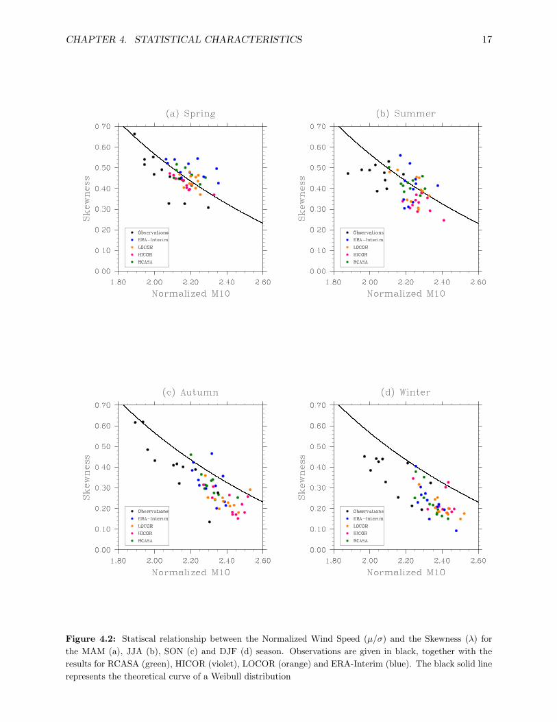
Analyzing the statistical relationship between the normalized wind speed, equal to the mean windspeed (µ) divided by the standard deviation (σ), and the skewness (λ), reveals more of the proper-ties of the probability distributions and might explain where differences between the models and theobservations arise. The normalized wind speed yields information on the width of the distribution,while the skewness defines the asymmetry of the distribution. A positive value for the skewnesscorresponds with a PDF which is tilted towards positive anomalies. The relationship between bothstatistical parameters can be used to define the nature of the profile. A commonly used PDF forwind speed modeling is the Weibull distribution (Pavia & O’Brien, 1986). This kind of distribu-tion has its own characteristical relationship between the normalized wind speed and the skewness,depending on its shape and scale parameter. When the PDF of one of the model runs yields askewness which is similar to the observations, but has a much larger (smaller) normalized windspeed, then we know that the shape, and therefore the physical meaning of the distribution is moreor less similar, but the model suffers from a consistent positive (negative) bias. When the skewnessalso alters, this indicates that inconsistencies that occur between the model and the observationsare not solely due to a constant over- or underestimation, but rather shield in the physics of thewind field. For this analysis, similar to that performed by He et al. (2010) and Monahan et al.(2011), we have separated the four seasons, i.e. spring (MAM), summer (JJA), autumn (SON)and winter (DJF). This way, we are able to study whether pronounced differences arise in specificseasons or under particular conditions.
CHAPTER 4. STATISTICAL CHARACTERISTICS 17
Figure 4.2: Statiscal relationship between the Normalized Wind Speed (µ/σ) and the Skewness (λ) forthe MAM (a), JJA (b), SON (c) and DJF (d) season. Observations are given in black, together with theresults for RCASA (green), HICOR (violet), LOCOR (orange) and ERA-Interim (blue). The black solid linerepresents the theoretical curve of a Weibull distribution

CHAPTER 4. STATISTICAL CHARACTERISTICS 18
In Figure 4.2, all results are given, where colours represent the respective data sets and modelruns as before for all stations. The black line indicates the theoretical curve of the Weibull dis-tribution, as a reference profile. As we can see in all four seasons, the observations (black dots)are positioned along the solid line, but are somewhat lower, on average. The Weibull distributionoverestimates the skewness of the distributions. This is most clearly visible in the results for theautumn (SON) and winter (DJF). Considering the model results, we note a distinct difference be-tween spring (MAM) and all other seasons. In springtime, results for all runs are relatively close toeach other. Especially the HICOR is very consistent over the range of all eleven stations. RCASAand LOCOR have a slightly higher normalized wind speed, on average. This is mostly due tothe higher mean 10m wind speed. Results for the model runs and for ERA-Interim are clusteringaround the Weibull distribution, and therefore overestimate the skewness of the observations as well.
During the rest of the year, the results show different features. In comparison with the models,the observations have a more positive skewness and a smaller normalized wind speed, in general.ERA-Interim remains closest to the observations throughout the year, due to a comparable meanM10, but its distributions are in general too tight, hence the larger normalized wind speed. Resultsfor RCASA are close to the actual measurements as well, but show an typical overestimation and aless skewed distribution at most of the stations. HICOR and LOCOR show the least resemblancewith the observations. HICOR is in general furthest away from the truth, with greater normalizedwind speeds as well as lower skewnesses. Interestingly enough, the results of all data sets com-bined follow the Weibull distribution rather closely. One could represent the models by a Weibulldistribution very well indeed, but the shape and scale parameter need to be adjusted to fit therespective model run, changing the characteristics of the distribution profile. The fact that boththe normalized wind speed and the skewness alter, indicates that the differences as seen betweenthe models and the observations are not solely due to a positive or negative bias. Taking that themean of the PDF is approximately equal for the three model runs and the observations, especiallyin the southern part of the North Sea, an increase in the normalized wind speed has to be dueto a decrease in the standard deviation. Together with this tendency towards somewhat smallerdistributions, the skewness, and therefore the asymmetry of the PDF, has decreased. Since thePDF’s in Figures 3.4a and d show no major differences in the lower part of the wind speed range,the former results imply that the tail of the observations’ distribution profile is longer and higherwind speed extremes are more common than the models predict.
A plausible cause for the clustering of the model results during the spring season, in contrastwith the spreading out of the results in winter and autumn, is the seasonal evolution of the windstorm frequency over the North Sea region, showing an increased number of wind storm eventsfrom November to February and a relatively low amount of storms during March, April and May(Renggli et al., 2012). These wind storm events act in the upper part of the wind speed range.This coincides with the idea that any differences that are present arise from the tail of the profile,the wind speed extremes. To indicate whether this is truly the case, we selected the upper 90th

CHAPTER 4. STATISTICAL CHARACTERISTICS 19
percentile of the wind speed data sets and derived both the mean and variance of this upper partof the spectrum. Results for all model runs and all stations are shown in Table B.2 of Appendix B.All stations show the same characteristics, where the mean value of the upper part of the spectrumis (much) lower for the observations than the RCASA or CORDEX runs show. In this respect,the ERA-Interim yields better correspondence with the measurements, but this is mainly due to atypical underestimation of the M10 in the full wind speed range. This is clear when we comparethe variance of the profile, which is widely underestimated by the reanalysis data. The observationsindicate that the spread of the upper part of the profile is relatively large, while the model runshave a tendency to cluster the more extreme wind speeds around a higher mean. For the formerRCA model (RCA3) it was concluded that the high wind speed end of the distribution is in generalunderestimated (Samuelsson et al., 2011). This is only partly true for the RCA4 model, sincethe mean of the upper 90th percentile is typically overestimated, but the extent of the high windspeed end is in all cases underestimated with respect to the actual observations. In light of furtherstudy, we would like to suggest to select multiple storm events and synchronize the instantaneouslymeasurement frequency of the stations with the model output and evaluate the distribution of thehigh-wind speed end of the PDF profile more carefully.
Chapter 5
Stability Conditions
Information on the stability conditions of the boundary layer is of major importance for climatemodelling. It is the layer where the exchange of momentum, heat, moisture and CO2 takes place,which is essential for the global and regional climate, as well as offshore generation of wind power(Pena, 2008). How the wind field behaves in the lower parts of the boundary layer depends largelyon the stability conditions. Therefore, we define three separate stability regimes, based on thestatic stability and vertical lapse rate.
5.1 Stability Regimes
The static stability can be roughly divided into stable, conditionally unstable and unstable con-ditions. The criterion in this study is based on the vertical temperature profile, the lapse rate.In the LOCOR run, the vertical levels are defined by unequally spaced hybrid terrain-followinglevels (Simmons and Burridge, 1981). This implies that the pressure level of each vertical level isvarying both in space and time. To define the stability, we selected the four lowest vertical levels,covering approximately the lowest 50 hPa of the boundary layer. For the RCASA and HICOR run,due to limited time, we made use of a more straightforward analysis, where set pressure levels areused. The lapse rate in both models has therefore been calculated between sea level and 925 hPa.The three regimes are set by a typical saturated adiabatic lapse rate and the dry adiabatic lapse rate:
Stable: γ < 4.0 K/km
Conditionally Unstable: 4.0 ≤ γ ≤ 9.8 K/km
Unstable: γ > 9.8 K/km
Since the observations, in all cases, only include the near-surface wind speed components andtherefore give no information on the static stability of the atmosphere, it is impossible to definethe appropriate stability regimes from the observations alone. In order to do so, we calculatedthe stability by means of the temperature lapse rate from the ERA-Interim reanalysis data andapplied this to our observations. The lapse rate has been calculated between sea level and 925 hPa,
20

CHAPTER 5. STABILITY CONDITIONS 21
Figure 5.1: Probability density functions for the 10m wind speed at the Ekofisk station under differentstability conditions. Stable is indicated by the yellow line, conditionally unstable by the green line andunstable by the blue line. The black line indicates the PDF for all recorded M10’s in the period from1988-1998. Results are shown for (a) Observations, (b) RCASA, (c) HICOR and (d) LOCOR

CHAPTER 5. STABILITY CONDITIONS 22
similar to RCASA and HICOR. This has been done for the period from 1988 to 1998, and to beable to make the conversion from reanalysis to observation data, we restricted ourselves to stationswith continous data for that time period, with wind field measurements at least every six hours.This narrows the number of appropriate stations down to four, i.e. Europlatform, K13, Ekofiskand Gullfaks. In this chapter, results are shown for the Ekofisk station, which in this sense actas a graphical reference, since the results for the three other stations show great resemblance withEkofisk.
Figure 5.1 shows the PDF’s for the defined stability regimes for the observations, the RCASArun and both CORDEX runs. Differences that were not visible by looking at the combinationof all data points arise when focusing on the separate boundary layer conditions. Regarding the(conditionally) unstable regime, we instantly note the similarity between the observations and theRCASA and HICOR run, both in terms of shape and scale of the distribution function. The LO-COR run, however, shows a pronounced rightward shift, indicative for overall higher wind speedsand a higher mean M10. Although the HICOR and LOCOR run yield seemingly equal results forthe time series in Figure 3.1 and for the PDF of all wind speeds indicated by the black line inFigure 5.1, there is a clear positive bias included in the lower-resolution run, in comparison withthe observations. The opposite is true for the stable regime, which yields only minor differences incase of the RCASA and HICOR run, but shows a leftward shift of the profile in LOCOR and inthe measurements. Under stable conditions, the LOCOR run appears to follow the observationsmore closely.
5.2 Sea Level Pressure Field
There is reason to believe that errors in the RCA4 model runs under different stability conditionsare due to an insufficient representation of synoptic and smaller scale weather features. Frictionwith the surface and curving of the isobars will have a pronounced effect on the wind field andtherefore need to be captured accurately. To make sure that the pressure field has been simulatedwell enough, we first have to ensure ourselves that all model runs yield approximately the samesea level pressure (SLP) range. Therefore, Figure 5.2 shows the probability density function forthe SLP over the period from 1988 to 1998 at the Ekofisk station. We note that the RCASA andLOCOR behave best in the lower pressure range, left of the peak at 1018 hPa. The HICOR shows aslight negative bias of about 3-5 hPa in this lower region, but yields a much better correspondencewith the observations in the high-pressure end of the distribution. Altogether, these differencesare presumably not too pronounced to disturb the SLP-field in general, but it is worthwhile toexamine the striking difference between the RCASA/LOCOR and higher resolution HICOR run.For now, we focus on the relation between the 10m wind speed and the sea level pressure as givenin Figure 5.3, where we have used the SLP-field of the ERA-Interim reanalysis, which is assumedto be a good representation of the actual pressure field. Since the number of points shared underthe unstable regime is much lower for the observations at the Ekofisk station (648) than for themodel runs (2038 - 2499), we decided to combine the unstable and conditionally unstable regime

CHAPTER 5. STABILITY CONDITIONS 23
Figure 5.2: Probability density function of the sea level pressure at the Ekofisk station from 1988 to 1998.Observations are represented by the black line, together with the results for RCASA (green), HICOR (violet)and LOCOR (orange)
to form one overall unstable regime. The difference in the size of the regimes might be due to theusage of different pressure levels to calculate the lapse rate. The all-including unstable regime isindicated by the blue markers, while the smaller stable regime is indicated by the yellow markers.In order to clarify the relation between the M10 and the SLP, regression lines are added to thescatter plots in Figure 5.3. The coefficients, corresponding to these regression lines, are given inTable 5.1. This includes the t-statistic value, indicative for the slope of the line, the standard errorof the regression coefficient, the intercept of the y-axis at x = 0 and the number of points in eachregime. For this latter analysis, the sea level pressure is set to Pa, rather than hPa.
The results yield a couple of interesting features in both stability regimes. While we noted arelatively pronounced overestimation of the wind speed for (conditionally) unstable conditions inLOCOR, the relationship between the pressure and the wind speed in this lower resolution modelrun shows great similarities with the observations. Low-pressures are clearly associated with higherwind speeds. The shape of the cloud of measurement points at Ekofisk is also directed towards thebottomright corner. The same pattern follows from analyses of the other three stations, taken intoaccount. Both RCASA and HICOR show some correlation as in the observations, but to a muchlesser extent. Although the PDF profile showed no distinct differences, it seems that both runs areunable to represent the pressure-wind speed relation accurately. This latter conclusion is not onlytrue for the (conditionally) unstable regime, but also under stable conditions, the pattern in Figure5.3 is somewhat different. Again, the observations show a clear correlation between lower pressuresand higher wind speeds, albeit with higher SLP’s, on average. The higher resolution runs show

CHAPTER 5. STABILITY CONDITIONS 24
Figure 5.3: Relationship between the 10m wind speed (x-axis) and the sea level pressure (y-axis) underdifferent stability conditions at the Ekofisk station. Stable (unstable) conditions are indicated with theyellow (blue) dots. Results are shown for (a) Observations, (b) RCASA, (c) HICOR and (d) LOCOR

CHAPTER 5. STABILITY CONDITIONS 25
Table 5.1: Regression Coefficients Ekofisk
Name t-statistic std. error y-intercept no. of points
Unstable
Observations -37.233 2.6571 101938.0 11924RCASA -9.7604 2.7728 101427.5 13152HICOR -6.4443 2.8228 101142.9 13340LOCOR -35.668 2.7418 102093.8 13787
Stable
Observations -14.471 4.4785 102305.7 3100RCASA -0.5590 4.7196 101775.3 2908HICOR 3.51630 5.1556 101533.4 2724LOCOR -15.825 6.7214 102472.9 2278
a much larger spread of the wind speed, where higher wind speeds are weakly related to higherpressure (HICOR) or are basically unrelated (RCASA). Since this characteristic is not present inthe LOCOR run, it is presumably related to rather small-scale features. The higher the horizontalresolution, the lesser the correspondence with the observations under unstable and stable conditions.Possible reasons for the inconsistencies between model runs and observations are to be found inthe turbulent kinetic energy (TKE) budget. Wind shear (drag) and buoyancy (vertical motions)effects are two important components of the TKE budget. In stable conditions, the amount of TKEresults from a competition between wind shear, which tends to produce turbulence, and buoyancy,which tends to suppress it. For unstable conditions, both effects act to produce turbulence. SinceHICOR runs with a higher Charnock constant than RCASA, the wind shear effect is ought tobe larger in the former run. This causes the production of turbulent energy to be larger, understable and unstable conditions. The results from both Figures 5.1 and 5.3, however, show no signof any significant differences between both runs in this respect. This implies that the buoyancydestruction or production of TKE is also larger in the HICOR run. Since both the RCASA andthe HICOR run are unable to represent the truth at multiple locations over the North Sea, it ishighly recommended, from a modelling perspective, to further study the effect of both wind shearand buoyancy on the TKE budget in both model runs in depth.

Chapter 6
Discussion & Recommendations
In this study, we have evaluated the performance of the RCA4 model in describing the wind fielddistribution over the North Sea, in comparison with station observations. These observations areretrieved from oil platforms, light ships and from an offshore wind farm. The reliability and accu-racy of those measurements is as ever questionable. The measurement height is different for everysource and converting the results to the 10m wind speed does include insecurities. Moreover, dueto maintenance, mechanical failures or malfunctioning of the equipment, observation time seriesare in cases irregularly interrupted or unsuitable. Regarding the eleven stations used for this study,much as possible has been done to select the stations such, that most of the North Sea region iscaptured with consistently measured time series of at least 7 years. Fortunately, in most regions,except for the Dutch waters, measurements originate from different sources, yielding a comparativecheck on accuracy. It is comforting to note, that variation in the observations are mostly relatedto the region, rather than the source of retrieval.
A first, basic analysis of the M10 time series, showed very consistent positive biases for bothCORDEX runs as well as for the RCASA run, especially in the central-northern region of theNorth Sea. The same is true for the general direction of the wind, which has the tendency to bemore north-westerly in all simulations, with slightly better correspondence of RCASA with theobservations. Much of this difference is observed in the ageostrophic component of the wind. Thislatter conclusion is mostly based on the difference with reanalysis data, which is thought to yielda good representation of the surface pressure field and the geostrophic wind component. For fur-ther study on the effect of the centrifugal and frictional force on the ageostrophic component, itwould be meaningful to use actual observations, if possible. Nevertheless, the cross-correlations ofall individual model runs with the actual measurements indicate that the temporal evolution (thetrend) in all simulations is very accurate. It is promising to note that the RCA4 model is capableto significantly improve on the ERA-Interim reanalysis results, on which it is initially driven.
Description of the statistical characteristics is indicative for the nature of the wind field. Ide-ally, one would use a model frequency similar to that of the measurements, to ensure that onecompares the exact same amount of data points over a specific period of time. Unfortunately, the
26

CHAPTER 6. DISCUSSION & RECOMMENDATIONS 27
modelling frequency was limited and the frequency of the observations varied significantly, depend-ing on the source. Nevertheless, general probability density functions of the M10 showed similarpatterns as the time series, with a distinct difference between the southern and central-northernregion, especially in the RCASA run. Analysis of the normalized wind speed, in relation with theskewness of the PDF, lead to the conclusion that all model results can be described by a slightlyless skewed Weibull distribution. However, for each model run, both the shape and scale parameterare to be adjusted. This implies that the distribution characteristics are different for each runand inconsistencies are not solely due to a negative or positive bias. Especially in the upper endof the distribution, models show much smaller variances, accompanied with higher means, thanobservations depict. From a modelling perspective, it is therefore very interesting to focus on themore extreme wind speeds in further analysis.
With the separation of the datasets in three stability regimes, differences and constraints of therespective model runs were further clarified. Although the LOCOR run appears to include a sys-tematic overestimation in the (conditionally) unstable regime, its high correspondence with theobservations, in terms of the relation between sea level pressure and 10m wind speed, is striking.For the RCASA and HICOR run inconsistencies arise in both the unstable and the stable regime.The effect of surface stress, related to the altered Charnock constant, is not fully exposed, due tothe additional effect of horizontal resolution. It is therefore highly recommended to run the RCA4model on a set resolution and adjust solely the Charnock constant. This will most likely revealmuch more of the physical consequences of the surface drag, both in terms of the wind speed profilein the surface layer and the production of turbulent kinetic energy. Additionally, a study to theproduction (destruction) of turbulence by buoyancy under unstable (stable) conditions is ought tobe worthwile. Solving the TKE budget gives information on the way that models solve small-scaleatmospheric features and can eventually lead to a more physical understanding of the processes athand.
Altogether, we believe that this study has been able to point out some striking differences betweenthree model runs, where increasing or decreasing the horizontal resolution as well as adjusting theCharnock constant seem to affect the results in a counter-intuitive manner. Therefore, in depthstudy on the physical mechanisms behind vertical mixing, surface drag, extreme wind speeds anddirectional shifts in the marine atmospheric boundary layer is thought to be of great value andinterest. We would suggest to increase the number of observational datasets, if possible, and ex-tend the study area to include possibly the Baltic Sea as well as coastal and onshore regions. Thiswill decrease the uncertainty that comes with the use of offshore measurements and it will enhanceunderstanding of the influence of surface drag, topography and geostrophy on the near-surface windfield.
References
[1] Capps, S. B. & C. S. Zender, 2009. Global Ocean Wind Power Sensitivity to Surface Layer Stability, Geophys.
Res. Lett., 36: L09801.
[2] Charnock, H., 1955. Wind Stress over a Water Surface, Quart. J. Roy. Meteorol. Soc., 81: 639-640.
[3] Dai, A. & C. Deser, 1999. Diurnal and Semidiurnal Variations in Global Surface Wind and Divergence Fields,
J. Geophys. Res., 104: 31109-31125.
[4] Gibescu, M., B. C. Ummels & W. L. Kling, 2006. Statistical Wind Speed Interpolation for Simulating Aggre-
gated Wind Energy Production under System Studies, Electrical Power Systems Laboratory, Delft University
of Technology.
[5] He, Y., A. H. Monahan, C. G. Jones, A. Dai, S. Biner, D. Caya & K. Winger, 2010. Probability Distributions
of Land Surface Wind Speeds over North America, J. Geophys. Res., 115: D04103.
[6] Hirata, Y., D. P. Mandic, H. Suzuki & K. Aihara, 2008. Wind Direction Modelling Using Multiple Observation
Points, Phil. Trans. R. Soc. A., 366: 591-607.
[7] Jagger, T., J. B. Elsner & X. Niu, 2001. A Dynamic Probability Model of Hurricane Winds in Coastal Counties
of the United States, J. Appl. Meteorol., 40: 853-863.
[8] Jones, C. G., U. Willen, A. Ullerstig & U. Hansson, 2004. The Rossby Centre Regional Atmospheric Climate
Model Part I: Model Climatology and Performance for the Present Climate over Europe, Ambio, 33: 199-210.
[9] Kunz, M., S. Mohr, M. Rauthe, R. Lux & Ch. Kottmeier, 2010. Assessment of Extreme Wind Speeds from
Regional Climate Models - Part I: Estimation of Return Values and Their Evaluation, Nat. Hazards Earth
Syst. Sci., 10, 907-922.
[10] Landberg, L., L. Myllerup, O. Rathman, E. L. Petersen, B. H. Jørgensen, J. Badger & N. G. Mortensen,
2003. Wind Resource Estimation: An Overview, Wind Energy, 6: 261-271.
[11] Luhar., A. K., P. J. Hurley & K. N. Rayner, 2009. Modelling Near-Surface Low Winds over Land under
Stable Conditions: Sensitivity Tests, Flux-Gradient Relationships and Stability Parameters, Boundary-Layer
Meteorol., 130: 249-274.
[12] Monahan, A. H., 2004. A Simple Model for the Skewness of Global Sea Surface Winds, J. Atmos. Sci., 61:
2037-2049.
[13] Monahan, A. H., 2006a. The Probability Distribution of Sea Surface Wind Speeds. Part I: Theory and Sea
Winds Observations, J. Clim., 19: 497-520.
[14] Monahan, A. H., 2006b. The Probability Distribution of Sea Surface Wind Speeds. Part II: Dataset Intercom-
parison and Seasonal Variability, J. Clim., 19: 521-534.
[15] Monahan, A. H., Y. He, N. McFarlane & A. Dai, 2011. The Probability Distribution of Land Surface Wind
Speeds, J. Clim., 24: 3892-3909.
[16] Morgan, E. C., M. Lackner, R. M. Vogel & L. G. Baise, 2011. Probability Distributions for Offshore Wind
Speeds, Energy Conv. and Mgmt., 52: 15-26.
[17] Nikulin, G., E. Kjellstrom, U. Hansson, G. Strandberg & A. Ullerstig, 2011. Evaluation and Future Projec-
tions of Temperature, Precipitation and Wind Extremes over Europe in an Ensemble of Regional Climate
Simulations, Tellus, 63A: 41-55.
28
REFERENCES 29
[18] Pavia, E. G. & J. J. O’Brien, 1986. Weibull Statistics of Wind Speed over the Ocean, J. Clim. and Appl.
Meteorol., 25: 1324-1332.
[19] Pena, A. & S-E. Gryning, 2008. Charnock’s Roughness Length Model and Non-Dimensional Wind Profiles
over the Sea, Boundary-Layer Meteorol., 128: 191-203.
[20] Pena, A., S-E. Gryning & C. B. Hasager, 2008. Measurements and Modelling of the Wind Speed Profile in
the Marine Atmospheric Boundary Layer, Boundary-Layer Meteorol., 129: 479-495.
[21] Petersen, E. L., N. G. Mortensen, L. Landberg, J. Højstrup & H. P. Frank, 1998a. Wind Power Meteorology.
Part I: Climate and Turbulence, Wind Energy, 1: 25-45.
[22] Petersen, E. L., N. G. Mortensen, L. Landberg, J. Højstrup & H. P. Frank, 1998b. Wind Power Meteorology.
Part II: Siting and Models, Wind Energy, 1: 55-72.
[23] Pryor, S. C. & R. J. Barthelmie, 2003. Long-Term Trends in Near-Surface Flow over the Baltic, Int. J.
Climatol., 23: 271-289.
[24] Pryor, S. C., R. J. Barthelmie, E. Kjellstrom, 2005. Potential Climate Change Impact on Wind Energy
Resources in Northern Europe: Analysis Using a Regional Climate Model, Clim. Dyn., 25: 815-835.
[25] Pryor, S. C., G. Nikulin & C. G. Jones, 2012. Influence of Spatial Resolution on Regional Climate Model
Derived Wind Climates, J. Geophys. Res., 117: D03117.
[26] Renggli, D., G. C. Leckebusch & U. Ulbrich, 2008. Seasonal Predictability of European Wind Storms, Institute
of Meteorology, Free University of Berlin.
[27] Samuelsson, P., C. G. Jones, U. Willen, A. Ullerstig, S. Gollvik, U. Hansson, C. Jansson, E. Kjellstrom,
G. Nikulin & K. Wyser, 2011. The Rossby Centre Regional Climate Model RCA3: Model Description and
Performance, Tellus, 63A: 4-23.
[28] Sjoblom, A. & A-S. Smedman, 2002. The Turbulent Kinetic Energy Budget in the Marine Atmospheric Surface
Layer, J. Geophys. Res., 107: no. C10, 3142.
[29] Simmons, A. J. & D. M. Burridge, 1981. An Energy and Angular Momentum Conserving Finite-Differences
Scheme and Hybrid Vertical Coordinates, Mon. Wea. Rev., 109: 758-766.
[30] Weisse, R. & F. Feser, 2003. Evaluation of a Method to Reduce Uncertainty in Wind Hindcasts Performed
with Regional Atmosphere Models, Coastal Engineering, 48: 211-225.
weblinks:
[31] DEWI GmbH, 2008. FINO 1 - Offshore Research Platform, http://www.dewi.de/dewi/index.php?id=152,
seen on 02-05-2012.
[32] KNMI, 2011. KNMI Hydra Project: Wind Climate Assessment of the Netherlands,
http://www.knmi.nl/samenw/hydra, seen on 25-04-2012.
[33] Kupiainen, M., C. Jansson, P. Samuelsson, C. Jones, U. Willen, U. Hansson, A. Uller-
stig, S. Wang & R. Doscher, 2011. Rossby Centre Regional Atmospheric Model, RCA4,
http://www.smhi.se/en/Research/Research-departments/climate-research-rossby-centre2-552/rossby-centre-
regional-atmospheric-model-rca4-1.16562, seen on 17-04-2012.
[34] NWS, 2010. Jetstream, Origin of Wind, NOAA National Weather Service, seen on 05-07-2012.
[35] SMHI, 2011. SMHI Annual Report 2011, http://www.smhi.se/en/about-smhi, seen on 11-07-2012.
[36] US Dept. of Energy, 2012. Wind Powering America, http://www.windpoweringamerica.gov, seen on 09-05-
2012.
[37] Wang, S., 2012. First Results from the New SMHI Atmosphere-Ocean-Ice Model RCA4-NEMO,
http://www.smhi.se/forskning/forskningsomraden/klimatforskning/1.21126, seen on 10-04-2012.
Appendix A
Model Coordinates
Table A.1: Grid Cell Coordinates for Europe Region
Name RCASA HICOR LOCOR ERA-I. OBS
Latitude λ
Europlatform 110:112 231:233 57:58 31:32 51.99◦
K13 116:118 242:244 60:61 29:30 53.22◦
Ekofisk 131:133 271:273 67:68 24:25 56.50◦
Sleipner 140:142 289:291 72:73 22:23 58.40◦
Gullfaks 152:154 314:316 78:79 18:19 61.20◦
Frigg 147:149 303:305 75:76 20:21 59.93◦
Auk 131:133 272:274 67:68 25:26 56.40◦
North Cormorant 153:155 315:317 77:78 18:19 61.23◦
Deutsche Bucht 118:120 246:248 61:62 28:29 54.11◦
Elbe 1 118:120 245:247 61:62 28:29 54.00◦
FINO 1 118:120 246:248 61:62 28:29 54.02◦
Longitude φ
Europlatform 64:66 175:177 43:44 43:44 03.28◦
K13 65:67 177:179 44:45 43:44 03.22◦
Ekofisk 68:70 183:185 45:46 43:44 03.20◦
Sleipner 67:69 180:182 45:46 41:42 01.90◦
Gullfaks 70:72 188:190 46:47 41:42 02.30◦
Frigg 69:71 184:186 45:46 41:42 02.00◦
Auk 65:67 177:179 44:45 42:43 02.07◦
North Cormorant 68:70 183:185 45:46 40:41 01.15◦
Deutsche Bucht 77:79 200:202 49:50 49:50 07.26◦
Elbe 1 79:81 204:206 50:51 50:51 08.07◦
FINO 1 75:77 196:198 48:49 48:49 06.58◦
30

Appendix B
PDF Statistical Tables
Table B.1: PDF Statistics
Name RCASA HICOR LOCOR ERA-I. OBS
Mean µ
Europlatform 7.81428 8.44934 7.52141 6.94955 7.73804K13 8.56544 8.63626 8.50780 7.86746 7.97202
Ekofisk 9.00448 8.91484 8.86373 8.29368 7.78670Sleipner 9.15873 9.05848 9.03270 8.42640 8.24242Gullfaks 9.31994 9.06706 9.18463 8.58254 8.17568
Frigg 9.30224 9.09048 9.23424 8.46308 7.14935Auk 9.08367 9.02239 8.98370 8.31748 7.90747
North Cormorant 9.40519 9.13643 9.23827 8.59171 8.25003Deutsche Bucht 8.06714 8.41882 8.30507 7.49275 8.62546
Elbe 1 7.62529 8.12014 7.55953 6.54128 8.06694FINO 1 8.40906 8.59390 8.22372 7.90324 7.49908
Variance σ2
Europlatform 14.4035 14.9694 13.0370 10.8333 14.0760K13 15.7774 15.2721 15.0134 13.0819 15.3484
Ekofisk 16.9800 16.0278 15.9207 14.5283 15.9558Sleipner 18.0964 16.9658 16.9568 16.0084 17.7215Gullfaks 19.5764 18.2145 18.3647 17.4239 18.6255
Frigg 19.4464 18.1480 17.7778 16.9043 15.0525Auk 17.4189 16.4572 15.9879 14.9329 17.6785
North Cormorant 19.6739 18.1750 17.9394 17.1110 19.4337Deutsche Bucht 13.7608 14.3712 14.3950 11.5693 17.0444
Elbe 1 12.7438 13.4531 12.4324 8.76492 14.0732FINO 1 14.1127 14.4835 13.6184 12.7452 12.5704
31

APPENDIX B. PDF STATISTICAL TABLES 32
Table B.2: PDF Statistics (90th percentile)
Name RCASA HICOR LOCOR ERA-I. OBS
Mean µ
Europlatform 15.1907 15.7641 14.4855 13.3919 13.4667K13 16.1939 16.0302 15.8921 14.8429 12.8761
Ekofisk 16.8499 16.4394 16.4301 15.5585 13.2579Sleipner 17.2424 16.8025 16.8225 16.0536 15.7456Gullfaks 17.7663 17.2548 17.3228 16.6906 14.8077
Frigg 17.7095 17.2305 17.2062 16.3840 14.7317Auk 17.0183 16.6643 16.5510 15.7021 14.5175
North Cormorant 17.8978 17.3538 17.2770 16.6218 15.0711Deutsche Bucht 15.2498 15.5950 15.4846 14.0430 16.3527
Elbe 1 14.4982 15.0288 14.2516 12.3262 15.1928FINO 1 15.5597 15.7395 15.2740 14.6957 12.6136
Variance σ2
Europlatform 3.47446 3.18513 3.03033 2.57191 4.27451K13 3.52600 3.26082 3.16962 2.88246 5.55195
Ekofisk 3.82372 3.42924 3.47377 3.12119 6.32229Sleipner 3.92029 3.44709 3.75296 3.50836 4.66033Gullfaks 4.33970 3.94247 3.99097 4.31830 6.12487
Frigg 4.22649 3.90473 3.82811 3.93677 5.22770Auk 3.86519 3.68254 3.66200 3.38056 6.57946
North Cormorant 4.30121 4.05339 3.83725 4.20315 7.43923Deutsche Bucht 3.31212 3.47722 2.92703 2.74716 3.81215
Elbe 1 3.13886 3.36635 2.57124 2.37250 3.76326FINO 1 3.08480 3.22975 3.09709 2.61396 4.55215

Appendix C
NCL Scripts
In this section, two NCL scripts are presented, which can be used as guidance for further study.The scripts are commented and made as compact as possible. This means that the methods shownsare only for one station, the Europlatform, and only the RCASA run is shown. Both CORDEXand ERA-Interim data can be treated likewise, so these are not shown here. First script is used tocalculate the monthly, seasonal and annual averages and make a graphical representation of the timeseries. Also, the cross-correlation is calculated and can be used for further analysis. The secondscript deals with the statistical properties of the probability density function and the relationshipbetween the normalized wind speed and the skewness can be retrieved from this script.
33

APPENDIX C. NCL SCRIPTS 34
load "$NCARG_ROOT/lib/ncarg/nclscripts/csm/gsn_code.ncl"load "$NCARG_ROOT/lib/ncarg/nclscripts/csm/gsn_csm.ncl"load "$NCARG_ROOT/lib/ncarg/nclscripts/csm/contributed.ncl" begin ;;;;;;;;;;;;;;;;;;;;;;;;;;;;;;;;;;;;;;;;;;;;;;; ;;;; Script to analyse time series ;;;; Europlatform (51.999N;3.276E) ;;;; ;;;;;;;;;;;;;;;;;;;;;;;;;;;;;;;;;;;;;;;;;;;;;;; ;;;;;;;;;;;;;;;;;;;;;;;;;;;;;;;;;;;;;;;;;;; ; Read in RCA4 coupled data (1979 - 2010) ; ; Read in RCA4 over full period;;;;;;;;;;;;;;;;;;;;;;;;;;;;;;;;;;;;;;;;;;; ; Method is similar for CORDEX and ERA-Interim dir_rca4 = "/nobackup/rossby16/sm_danku/Scripts/" rca4_name = "RCA4_Europlatform.txt" data_rca4 = asciiread(dir_rca4+rca4_name,-1,"string")m10_rca4_ave = stringtofloat(str_get_cols(data_rca4,0,8)) ; 10m wind speed, averaged over grid cellsmonth_rca4 = stringtofloat(str_get_cols(data_rca4,15,16))year_rca4 = stringtofloat(str_get_cols(data_rca4,11,14)) ;; Calculate monthly mean over time series rca4_monthly = new(250,float) ; Array to hold all data for one monthrca4_mon_mean = new(384,float) ; Array to hold all monthly means i = 0j = 1n = 1979k = 0l = 0 do while(n.le.2010) j = 1 do while(j.le.12) k = 0 do while(month_rca4(i).eq.j .and. i.lt.93503) ; Similar method is applied for annual rca4_monthly(k)=m10_rca4_ave(i) ; and seasonal means
i = i+1k = k+1
end do rca4_mon_mean(l)=avg(rca4_monthly) l = l+1 j = j+1 end do n = n+1end do ;;;;;;;;;;;;;;;;;;;;;;;;;;;;;;;;;;;;;;;;;;; Read in observational data (1983-2005) ; ; Read in observations over measured period;;;;;;;;;;;;;;;;;;;;;;;;;;;;;;;;;;;;;;;;;; dir_obs = "/nobackup/rossby16/sm_danku/HYDRA_OBS/"obs_name = "Data/s321.txt" data_obs = asciiread(dir_obs+obs_name,-1,"string")year_obs = stringtofloat(str_get_cols(data_obs,0,3))month_obs = stringtofloat(str_get_cols(data_obs,4,5)) ddd_obs = stringtofloat(str_get_cols(data_obs,12,14)) ; 10m wind directionm10_obs = stringtofloat(str_get_cols(data_obs,20,22)) ; 10m wind speed ;; Calculate monthly mean over time series obs_monthly = new(750,float) ; Values per month, depending on frequencyobs_mon_mean = new(384,float) ; Array to hold all monthly means

APPENDIX C. NCL SCRIPTS 35
i = 0j = 1n = 1983 ; Starting year of measurementsk = 0l = 48 ; Starting month of measurements obs_monthly@_FillValue = 9.96921e+36 ; Fill value for missing or subzero wind speed do while(n.le.2005) j = 1 do while(j.le.12) k = 0
obs_monthly = obs_monthly@_FillValue do while(month_obs(i).eq.j .and. i.lt.201575) ; Similar method is applied for annual obs_monthly(k)=m10_obs(i) ; and seasonal means i = i+1 k = k+1 end do obs_mon_mean(l)=avg(obs_monthly) l = l+1 j = j+1 end do n = n+1end do ;;;;;;;;;;;;;;;;;;;;;;;;;;;;;;;;; Calculate cross-correlations ;;;;;;;;;;;;;;;;;;;;;;;;;;;;;;;;;
good = ind(.not.ismissing(rca4_seas) .and. .not.ismissing(obs_seas)) ; Match seasonal time series of model and obs.corr_rca4_obs = escorc(rca4_seas(good),obs_seas(good)) ; Calculate the corresponding cross-correlation ;;;;;;;;;;;;;;;;;;;;;;;;;;; Start graphics section ;;;;;;;;;;;;;;;;;;;;;;;;;;; wks = gsn_open_wks("pdf",dir_output+graph_name) ; Open workstation to draw plotplot = new(5,graphic) ; Create graphic interface plot0 = gsn_csm_xy(wks,years,rca4_ann_mean,res0) ; Plot time series with corresponding resourcesplot1 = gsn_csm_xy(wks,years,cor_ann_mean,res1)plot2 = gsn_csm_xy(wks,years,loc_ann_mean,res2)plot3 = gsn_csm_xy(wks,years,era_ann_mean,res3)plot4 = gsn_csm_xy(wks,years,obs_ann_mean,res4) gsres = Truegsres@gsFillColor = "gray85" dum1 = gsn_add_polygon(wks,plot2,years_obs,obs_std,gsres) ; Create grey shaded area for annual variance overlay(plot0,plot1) ; Overlay plots in single graphicoverlay(plot0,plot2)overlay(plot0,plot3)overlay(plot0,plot4) draw(plot0)frame(wks) ; Advance the plot in the workstation end
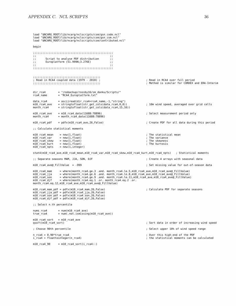
APPENDIX C. NCL SCRIPTS 36
load "$NCARG_ROOT/lib/ncarg/nclscripts/csm/gsn_code.ncl"load "$NCARG_ROOT/lib/ncarg/nclscripts/csm/gsn_csm.ncl"load "$NCARG_ROOT/lib/ncarg/nclscripts/csm/contributed.ncl" begin ;;;;;;;;;;;;;;;;;;;;;;;;;;;;;;;;;;;;;;;;;;;;;;;;;;;;; ;;;; Script to analyse PDF distribution ;;;; Europlatform (51.999N;3.276E) ;;;; ;;;;;;;;;;;;;;;;;;;;;;;;;;;;;;;;;;;;;;;;;;;;;;;;;;;;; ;;;;;;;;;;;;;;;;;;;;;;;;;;;;;;;;;;;;;;;;;;;; Read in RCA4 coupled data (1979 - 2010) ; ; Read in RCA4 over full period;;;;;;;;;;;;;;;;;;;;;;;;;;;;;;;;;;;;;;;;;;; ; Method is similar for CORDEX and ERA-Interim dir_rca4 = "/nobackup/rossby16/sm_danku/Scripts/"rca4_name = "RCA4_Europlatform.txt" data_rca4 = asciiread(dir_rca4+rca4_name,-1,"string")m10_rca4_ave = stringtofloat(str_get_cols(data_rca4,0,8)) ; 10m wind speed, averaged over grid cellsmonth_rca4 = stringtofloat(str_get_cols(data_rca4,15,16)) m10_rca4_ave = m10_rca4_data(11688:78896) ; Select measurement period onlymonth_rca4 = month_rca4_data(11688:78896) m10_rca4_pdf = pdfx(m10_rca4_ave,26,False) ; Create PDF for all data during this period ;; Calculate statistical moments m10_rca4_mean = new(1,float) ; The statistical meanm10_rca4_var = new(1,float) ; The variancem10_rca4_skew = new(1,float) ; The skewnessm10_rca4_kurt = new(1,float) ; The kurtosism10_rca4_npts = new(1,integer) stat4(m10_rca4_ave,m10_rca4_mean,m10_rca4_var,m10_rca4_skew,m10_rca4_kurt,m10_rca4_npts) ; Statistical moments ;; Separate seasons MAM, JJA, SON, DJF ; Create 4 arrays with seasonal data m10_rca4_ave@_FillValue = -999 ; Set missing value for out-of-season data m10_rca4_mam = where(month_rca4.ge.3 .and. month_rca4.le.5,m10_rca4_ave,m10_rca4_ave@_FillValue)m10_rca4_jja = where(month_rca4.ge.6 .and. month_rca4.le.8,m10_rca4_ave,m10_rca4_ave@_FillValue)m10_rca4_son = where(month_rca4.ge.9 .and. month_rca4.le.11,m10_rca4_ave,m10_rca4_ave@_FillValue)m10_rca4_djf = where(month_rca4.eq.1 .or. month_rca4.eq.2 .or. month_rca4.eq.12,m10_rca4_ave,m10_rca4_ave@_FillValue) m10_rca4_mam_pdf = pdfx(m10_rca4_mam,26,False) ; Calculate PDF for separate seasonsm10_rca4_jja_pdf = pdfx(m10_rca4_jja,26,False)m10_rca4_son_pdf = pdfx(m10_rca4_son,26,False)m10_rca4_djf_pdf = pdfx(m10_rca4_djf,26,False) ;; Select n.th percentile nums_rca4 = num(m10_rca4_ave)true_rca4 = num(.not.ismissing(m10_rca4_ave)) m10_rca4_sort = m10_rca4_aveqsort(m10_rca4_sort) ; Sort data in order of increasing wind speed ; Choose 90th percentile ; Select upper 10% of wind speed range n_rca4 = 0.90*true_rca4 ; Over this high-end of the PDFi_rca4 = floattointeger(n_rca4) ; the statistical moments can be calculated m10_rca4_90 = m10_rca4_sort(i_rca4::)

APPENDIX C. NCL SCRIPTS 37
;;;;;;;;;;;;;;;;;;;;;;;;;;; Start graphics section ;;;;;;;;;;;;;;;;;;;;;;;;;;; wks = gsn_open_wks("pdf",dir_output+graph_name) ; Open workstation to draw plotplot = new(5,graphic) ; Create graphic interface plot0 = gsn_csm_xy(wks,m10_rca4_pdf@bin_center,m10_rca4_pdf,res0) ; Plot PDF's with corresponding resourcesplot1 = gsn_csm_xy(wks,m10_cor_pdf@bin_center,m10_cor_pdf,res1)plot2 = gsn_csm_xy(wks,m10_loc_pdf@bin_center,m10_loc_pdf,res2)plot3 = gsn_csm_xy(wks,m10_era_pdf@bin_center,m10_era_pdf,res3)plot4 = gsn_csm_xy(wks,m10_obs_pdf@bin_center,m10_obs_pdf,res4) overlay(plot0,plot1) ; Overlay plots in single graphicoverlay(plot0,plot2)overlay(plot0,plot3)overlay(plot0,plot4) draw(plot0)frame(wks) ; Advance the plot in the workstation end

Appendix D
Self Reflection
This section includes what is possibly one the major aspects of this whole internship experience.The analyses have been performed, the results have been discussed and the report has been written,but how does one look back at the work that has been done and the knowledge and skills that havebeen gained. A self-reflection on the results of a scientific process as well as on the social adaptationto a new professional work environment is provided here.
At the dawn of the new year, the first contacts were established between me, Bert Holtslag (profes-sor Meteorology at Wageningen University) and Colin Jones (head of the Rossby Centre, SMHI).Two months before the start of my internship, we agreed upon the main theme of study for thisfour month period. Considering my special interest for oceanography and wind energy potential,we decided that the SMHI could benefit from a thorough evaluation of the offshore wind distribu-tion in their newly developed Rossby Centre Regional Climate Model RCA4. Though the precisecontent of the upcoming research internship was yet to be determined, the arrangements as saidgave already a good sense of direction and definitely enhanced my enthusiasm for the project. Thepersonal goals set for this internship were to get myself familiarized with working in a professionalscientific organisation, contribute to the research and development at the SMHI and to extendmy knowledge on the offshore wind field modelling and wind energy production over open-waterregions. Essentially, I was eager to find a balance between fundamental science and the practicalapplications of this research.
At the start of the internship, we discussed the research possibilities and narrowed the field ofstudy down to the Baltic and North Sea and decided to gather as much observational data as pos-sible to use as a comparison and quality measure for, initially, one run of the RCA4 model, whichis currently being analysed and improved. We agreed to focus on the near-surface wind speedand direction and try to analyse the nature of the wind field distributions by means of statisticalanalysis. The intention was to implement the wind energy potential of this regional climate modelin the study as well. However, it was already clear from the beginning that the greatest hurdle tobe taken was to gather a sufficient amount of reliable and consistently measured observational dataover the Baltic and North Sea. As it turned out, there were no offshore wind field time series over
38

APPENDIX D. SELF REFLECTION 39
the Baltic Sea which met our requirements, since coastal stations were excluded, due to the stronginfluence of nearby land surface areas. Therefore, we soon decided to shift our focus to the NorthSea solely. Although the gathering of these measurement was one of the major hassles during theinternship, this was one of the key areas where you notice the advantage of being involved in amajor meteorological institute with many direct contacts, provided by Colin Jones, mainly, whichlead to scientists from all over the world who all provided me with extra information, and mostimportantly, real data. Using the SMHI nametag also worked very efficiently to retrieve measure-ment data from a private wind energy company, when asked for a time series for scientific purposes.Alltogether, thanks to those allocated sources, I feel I managed to select a proper and suitable setof measurement data, which can be useful in more analyses as well.
Right from the beginning, I have tried to structurize and organize my data as much as possi-ble. Four months is a fairly short period of time, and you are constantly aware of the fact thatdeadlines will come in rather sooner than later. Therefore, I forced myself to learn the NCL pro-gramming language as efficiently as I could and make easily readable and editable scripts. Despiteall efforts, it was not a simple task to retain the structure in the used folders, due to the amountof station data, and especially due to the fact that every source delivered the data differently andevery set of data asked for a different method to obtain the atmospheric parameters needed. Itbasically meant I regularly had to clean my folders and documented the steps that I took and theresults that were produced. My supervisors gave me all the space and time that I needed to getmyself familiarized with the model and the observational data and awaited my first results withpatience. Although this created a relaxed atmosphere wherein I was allowed to make errors, I feltafter some time that I really needed a thorough discussion on the results and the way to interpretthem. This first meeting helped me to understand the results, motivated me to get into some moredetails on particular subjects and opened up the way for more discussion. Halfway through theinternship, I had a very productive gathering with all three supervisors, which gave me some freshideas how to further analyze the data, but was also the ideal opportunity to lay out the targets forthe remainder of the research period and to agree on my preconceived planning. I feel this meetingwas very helpful, not only for myself, but also for my supervisors, to know what they could expectfrom me the last months of my internship.
I believe that I benefited strongly from regularly making a suitable planning and setting cleartargets during this four month period. This definitely decreased the level of stress in the finalweeks of the internship. However, the greatest disadvantage of the reasonable short period of time,is that you are constantly looking beyond the internship and are at times occupied by what liesahead, that is, graduation and starting my professional career. I am very thankful for the libertythat I have been given to take some time off to apply for a couple of vacancies in the Netherlandsand to join a selection day in Rotterdam. Succesfully concluding this adventure gave me some peaceof mind for the last weeks of my stay in Sweden. It also stimulated me to succesfully complete myresearch and to come up with new analyses which would further expose differences between the(eventually) three applied runs from the RCA4 model and the observations, such that the SMHI

APPENDIX D. SELF REFLECTION 40
would really profit from my scientific work. Overall, I am glad with the results of this study andthe final report that has been composed. I believe that I have been able to show where differencesarise and what atmospheric parameters deserve greatest attention from a modelling perspective.Especially near the end of your stay, you observe some interesting features of the model wind field,which make you curious to know what is actually going on and to find out how one can explain thephysics behind the observed inconsistencies.
Regarding the personal goals, as described before, I think I managed to succeed in reaching myinternship objectives reasonably well. Although my research topic didn’t allow for many interac-tive work with other researchers, I had a good time enjoying the presence of an international mixof colleagues during lunch and coffee breaks. I had a great time following Swedish class, offeredthrough the SMHI, allowing me to get a feeling for the language and culture. Whether my workhas been of great value to the further model development at the SMHI is obviously subject todiscussion, which only time can tell. I do, however, feel that I have been able to spot some errorsas well as promising results and used some methods which can be applied further on as well. Itruly hope that the Rossby Centre will continue the research on the wind field distribution overoffshore and onshore regions and will eventually be able to improve their regional climate model.Though I extended my knowledge on the offshore wind field distribution, I would have liked to beable to focus more on the wind energy potential. I guess time was the critical factor, limiting thepossibilities to go further into this topic, next to the fact that the model is still to be evaluated andimproved on more essential points. It is of major importance to ensure ourselves of the accuracyof the model, before we study further possibilities and its practical applications. In the end, I amvery satisfied with this Scandinavian experience and I am very glad I took the chance to move toNorrkoping and hope to stay in contact and remain updated on the work performed at the SMHI.

Appendix E
About SMHI
SMHI is an abbreviation for Sveriges Meteorologiska och Hydrologiska Institut (Swedish Meteoro-logical and Hydrological Institute). Its head office is situated in Norrkoping, Ostergotland. SMHIis a government agency under the Ministry of the Environment, with approximately 660 employ-ees. The organisation has expertise within the areas of meteorology, hydrology, oceanography andclimatology and aims to provide social benefits by increasing safety and fostering a more sustain-able society (SMHI, 2011). SMHI manages and develops information that provides knowledge andadvanced decision-making information for public services. Some examples of those services areweather forecasting, warnings and statistics, climate studies, simulations and analysis, and con-tracted research. The SMHI works in extensive national as well as international cooperation andconsortia, such as the Global Monitoring for Environmental and Security programme.
The Institute provides a wide range of data and knowledge, including climate scenarios, indica-tors and various training programmes. It supports the Swedish government by providing expertiseon scientific questions connected with planning for the future as well as when UN climate negotia-tions are at hand. The SMHI has been involved in arranging various seminars and forums on climateissues. Every year, a Rossby Centre Day is held on climate modelling research. Furthermore, itsupports Sweden’s water management by creating accessible information that is operationally re-liable. Decision support tools are being developed to support attainment of the national clean airenvironment objective.
Based on the knowledge in the areas of climate, energy and the environment, the SMHI aimsto build competence to ensure better future decisions. The goal is to develop products and ser-vices that support the individual, region and country to achieve a promising future (SMHI, 2011).Therefore, the SMHI invests in modern applications, such as a mobile weather app for the generalpublic and a special farmer’s app describing critical weather conditions. Next to these businessservices, the SMHI provides training and education for various groups in how weather influencesbusiness for professional working in the areas of roads, energy, shipping and wind power.
41