evaluation of the intrinsic and extrinsic fracture

ONRL/Sub/95-ST547/02

Draft Final Report

EVALUATION OF THE INTRINSIC AND EXTRINSIC FRACTURE BEHAVIOR OF IRON

ALUMINIDES

October 15, 2001

Research sponsored by the U.S. Department of Energy, Office of Fossil Energy

Advanced Research and Technology Development Material Program

Report Prepared by Bernard R. Cooper and Bruce S. Kang

West Virginia University Dept .of Physics and Dept. of Mechanical & Aerospace Engineering

Morgantown, WV 26506-6315 under

19x-ST547C, WVU-2

for

OAK RIDGE NATIONAL LABORATORY Oak Ridge, Tennessee 37831

Managed by UT-BATTELLE, LLC

for the U.S. DEPARTMENT OF ENERGY

under contract DE-AC05-000R22725

2

EVALUATION OF THE INTRINSIC AND EXTRINSIC FRACTURE BEHAVIOR OF IRON ALUMINIDES

B.R. Cooper1 and B.S.-J. Kang 2 1 Physics Department

2 Mechanical and Aerospace Engineering Department West Virginia University Morgantown, WV 26506

ABSTRACT

Comparative finite element modeling simulations of initial intergranular fracture

of two iron aluminides (FA186 and FA189) were carried out to study the intrinsic and extrinsic fracture behavior of the alloys as related to hydrogen embrittlement. The computational simulations involved sequentially-coupled stress and mass-diffusion analyses to determine the stress/strain distribution and the extent of hydrogen concentration at the crack tip region. Simulations of initial intergranular fracture of the two alloys under either air or vacuum conditions were conducted. With judicious selection of grain boundary failure strains for each alloy and assumed material degradation at hydrogen diffusion zone, the numerical results agree well with previous experimental test results.

We have considered the various methods by which the thermal expansion of Fe3Al can be modeled. As a matter of practicality, we have started with a conceptually simple continuum medium modeling, which we have used in initial calculations reported here, despite its limitations in neglecting the effects of optical phonons. This makes the results increasingly suspect for temperatures above the Debye temperature. However, the results we obtain are surprisingly good considering this important limitation.

Nevertheless, we regard these results as being suspect. Therefore, in addition, we discuss a wholly new ab-initio-based method which is both more accurate (preserves the ab-initio-generated information) and computationally more efficient. This method can directly transform the all-electron ab initio electronic structure results of the full-potential LMTO electronic structure behavior, computationally provided in reciprocal space, to the real space representation needed for the thermal expansion modeling. An increase of computational speed, use of larger supercells, and more efficient calculations, can all be achieved by using real space (tight-binding (TB)) calculations. The TB parameters are obtained from direct Fourier transform of the matrix elements in momentum space for a specific structure and specific lattice constant. The parameters that may change significantly are the onsite parameters, which depend on the onsite electron density. To make a usable look-up table, good for variable lattice constant in the same structure, one can perform several runs with different lattice constants and obtain a fitting function of the onsite parameter as a function of lattice constant, for each orbital in each atom. We are at present implementing this method for initial application to Fe3Al before proceeding to a study of molybdenum silicide systems.

3

I. COMPUTATIONAL HYDROGEN EMBRITTLEMENT SIMULATIONS OF IRON ALUMINIDES

Motivation and Summary of Relevant Experimental Results

Comparative crack growth tests of two iron aluminides subjected to constant tensile loading in air were conducted at WVU [1]. The two selected iron aluminides are designated as FA186 with basic composition of Fe-28Al-5Cr at. % and FA189 with Fe-28Al-2Cr and an addition of 0.5 at. % Zr, 0.05 at. % C and 0.005 at. % B. The purpose of adding a small amount of boron in FA-189 was to improve the grain boundary cohesive strength such that intergranular failure can be minimized. However, with micro-alloying of B and Zr, FA-189 have much smaller grains. The estimated grain sizes are 193µm for FA186 and 75µm for FA189, respectively. Thus, intrinsically FA-189 should have higher fracture toughness than that of FA-186. However, as indicated by the experimental results [1], because of their smaller grain size, FA-189 is extrinsically more susceptible to environmental embrittlement than FA-186 under low strain loading condition. Table 1 shows the test matrix relevant to the computational modeling. Overall, the experimental results indicated that between the two alloys, the ternary alloy FA186 has the better fracture resistance, higher fracture toughness and smaller sensitivity to hydrogen embrittlement. Thus, to further investigate the effect of grain size, we carried out comparative finite element modeling simulations of intergranular fracture of FA186 and FA189, subjected to stress-assisted hydrogen embrittlement.

Finite Element Analysis Model

In this research, a finite element model coupled with a hydrogen diffusion model was developed to simulate the intergranular crack growth due to hydrogen embrittlement. The numerical analyses were carried out using the commercial finite element code ABAQUSTM. A submodeling technique was implemented to obtain detailed near-tip stress and strain fields by using a refined mesh for the area ahead of the crack tip. The crack-tip submodel is designed to represent qualitatively the grain sizes of FA186 or FA189. The concept of submodeling consists of performing two independent analyses, one on the global model with a coarse mesh, and the other on a locally refined mesh (submodel), with the only link being the transfer of interfacial boundary displacements. The nodal displacements of the global model are interpolated onto the boundary of the submodel providing a detailed solution in the area of interest. Due to the symmetry of loading, only half of the specimen size was modeled in the global model. This model consists of 1744 plane stress elements with a fine mesh in the region around the crack tip, as shown in Figure1. Near the crack tip region, two submodels were designed to represent qualitatively the grain size of FA186 and FA189, respectively. A multi-grain crack tip cell was used in the local finite element mesh composed of a periodic array of regular hexagonal grains. As shown in Figure 2, the hexagon used in the submodel for FA186 represents the typical grain size of 193µm and the submodel contains a total of 8,448 elements. The hexagon used for FA189 represents the typical grain size of 75µm and the submodel contains a total of 22,528 elements.

4

Validity Of Finite Element Submodeling

The first assumption made in modeling the grains and grain boundaries was that the grain boundary is weaker than the matrix. Also, due to the addition of small amount of B in FA189, the grain boundary cohesive strength of FA189 is stronger than that of FA186. According to this assumption, we chose the following Young’s modulus values: EGB (FA-186) = 40% E matrix = 40% * 1.41E+5 = 0.564E+5 MPa EGB (FA-189) = 70% E matrix = 70% * 1.41E+5 = 0.987E+5 MPa

The next assumption was needed to ensure that the submodeling approach will satisfy the (deformation) compatibility condition. A homogenization procedure based on the rule of mixture (ROM) was adopted in this study. In this approach, the heterogeneous material in the submodel (with two different Young’s modulus values for matrix and grain boundaries) is replaced with an equivalent homogeneous one having the same Young’s modulus values as that of the global model. The ROM formula was written in terms of area fractions, i.e. Esubmodel = Ematrix Amatrix + EGB AGB

where Amatrix (= area of grain elements / total area) is the area fraction of grains, and AGB (= area of grain boundaries / total area) is the area fraction of grain boundaries. The results of the Ematrix and EGB values obtained for FA186 and FA189 are shown in Table 2.

The validity of the proposed homogenization procedure and submodeling technique can be verified by examining the contour plots of principal strains near the interfacial boundaries of the submodeled region. As shown in Figure 3, which shows superimposed contour plots of principal strains of the global model and submodel, the compatibility condition is indeed satisfied.

Hydrogen Diffusion Model The hydrogen diffusion model is based on the concept of an elastic interaction between the hydrostatic pressure (or the volumetric component of a crack tip stress tensor) and the dilatation associated with an interstitial hydrogen atom [2]. The localization of hydrogen atoms can be explained by the effect of hydrostatic stress on the chemical potential of hydrogen atoms. For the simple case of spherical hydrogen, the enhanced hydrogen concentration by σii/3 in the region has been shown to follow Boltzman statistics

where C0 is the initial concentration and VH is the partial molar volume of hydrogen.

=

RT

VCC Hii

H 3exp0

σ

5

The governing equations for hydrogen diffusion used in ABAQUSTM are an extension of Fick’s equations: they allow for nonuniform solubility of the diffusing substance in the base material and for hydrogen diffusion driven by the gradient of pressure.

where J is the flux of concentration of the hydrogen gas, D is the diffusivity, S is the solubility of the hydrogen gas, Kp is the pressure stress factor and p is the pressure stress. In our analysis the basic solution variable (used as the degree of freedom at the nodes of the mesh) is the “normalized concentration” (often also referred to as the “activity” of the diffusing material) defined by φ = C/S, where C is the mass concentration of the diffusing hydrogen and S its solubility. This variable was chosen because the mesh includes dissimilar materials (i.e. different Young’s modulus values for grains and grain boundaries) and in this case the normalized concentration is continuous across the interface between the grain and grain boundary. Stress-assisted diffusion of hydrogen is specified by defining the pressure stress factor, Κp, using the analytical solution presented by Liu [3], as

where R = 8.31432 J/molK is the universal gas constant, VH = 2.0×103 mm3/mol is the partial molar volume of hydrogen in iron-based metals.

Finally, the following material properties are selected for the computational calculations [4].

where S is the solubility expressed in atoms of H2 gas per m3 of iron, P is the partial pressure of hydrogen gas and T the is temperature. For this research, we set P = 1 atm and T=300K. Note that the initial concentration is dictated by Sievart’s law: C = P1/2× S The crack surface is assumed to be “open” and to allow equilibration with the hydrogen gas, such that the dominant process will be the transport of hydrogen from the crack tip. A steady state hydrogen diffusion analysis is conducted and the rate of change of concentration with respect to time is omitted from the governing equations.

( )zH

P R

VK

θθφ

−=

−×=

−−

RTkJmol

sm

D12

7 88.6exp1010.2Diffusivity:

,28

exp10989.11

26

−×=

−

RTkJmol

PSSolubility:

.C p

J D SKpx x

∂ ∂ =− ⋅ + ∂ ∂

6

Steps Of Simulating Intergranular Fracture Due To Hydrogen Embrittlement

(1) Finite element stress/strain analysis of the global model, (2) Finite element stress/strain analysis of the submodel at the crack-tip region, (3) Steady state hydrogen diffusion analysis based on the hydrogen diffusion model coupled with the results from step (2), (4) Degrade the material properties in the high hydrogen concentration zone in submodel, (5) Finite element stress/strain analysis of the updated specimen configuration (similar to steps (1) and (2)), (6) Apply maximum principal strain failure criterion and simulate intergranular crack growth, (7) Go to step (1) and repeat the cycle. For this simulation, it is assumed that a material degradation will occur at the stress-assisted hydrogen concentration region. Accordingly, the material property (Young’s modulus in this analysis) is reduced both at the matrix and grain boundary region by the following formula:

Normalized concentration ratio % of reduction of Young’s modulus 1 to 3 20 % 3 to 6 30 % 6 to 10 40 % 10 to 15 50%

After degrading the material properties, a new static analysis of the submodel is carried out to determine the updated crack tip stress/strain state; and, based on the selected failure strains for FA186 and FA189, the possibility of intergranular cracking is evaluated and proper boundary conditions in the crack tip submodel region are then adjusted. A failure strain of 4% for FA186 and a failure strain of 6% for FA189 are selected in this numerical analysis. Because both the geometric configuration and material properties in the submodel were changing with the updated crack growth, it is necessary to satisfy the compatibility of displacements at the interfacial boundary region. This was accomplished by updating the crack length in the global model together with modifying the elastic modulus of the elements in the global model corresponding to the submodel area. This was done at every three to four steps at which the new Young’s modulus of the submodel was determined based on the rule of mixture approach and modified material properties of grains and grain boundaries, as shown in Figure 4.

Results and Discussions

Table 3 shows the finite element simulation matrix. As shown, a total of 12 comparative finite element simulations under vacuum and air at two different stress intensity factors and two different failure strains were carried out in this research. Figures 5 and 6 show examples of intergranular crack growth due to hydrogen embrittlement for FA186 under applied stress intensity factors of 17.36 MPa√m and

7

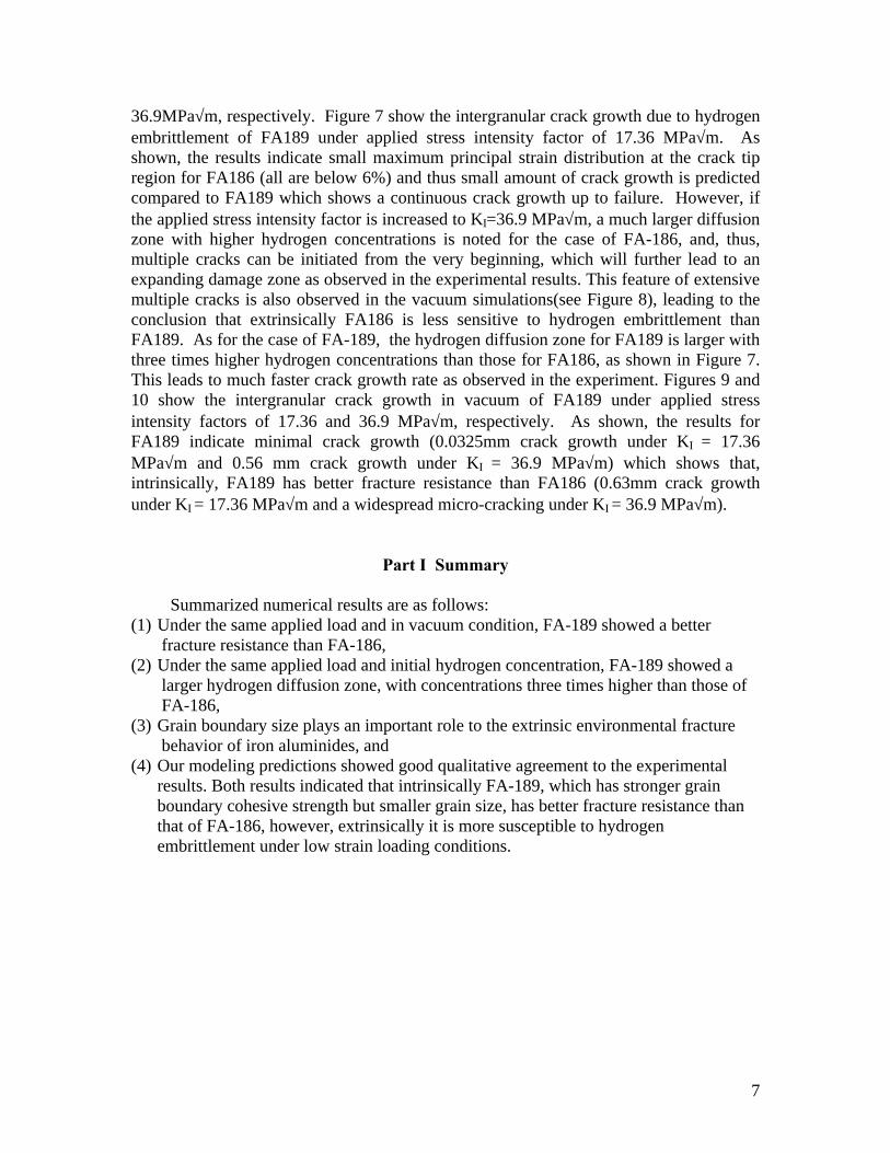
36.9MPa√m, respectively. Figure 7 show the intergranular crack growth due to hydrogen embrittlement of FA189 under applied stress intensity factor of 17.36 MPa√m. As shown, the results indicate small maximum principal strain distribution at the crack tip region for FA186 (all are below 6%) and thus small amount of crack growth is predicted compared to FA189 which shows a continuous crack growth up to failure. However, if the applied stress intensity factor is increased to KI=36.9 MPa√m, a much larger diffusion zone with higher hydrogen concentrations is noted for the case of FA-186, and, thus, multiple cracks can be initiated from the very beginning, which will further lead to an expanding damage zone as observed in the experimental results. This feature of extensive multiple cracks is also observed in the vacuum simulations(see Figure 8), leading to the conclusion that extrinsically FA186 is less sensitive to hydrogen embrittlement than FA189. As for the case of FA-189, the hydrogen diffusion zone for FA189 is larger with three times higher hydrogen concentrations than those for FA186, as shown in Figure 7. This leads to much faster crack growth rate as observed in the experiment. Figures 9 and 10 show the intergranular crack growth in vacuum of FA189 under applied stress intensity factors of 17.36 and 36.9 MPa√m, respectively. As shown, the results for FA189 indicate minimal crack growth (0.0325mm crack growth under KI = 17.36 MPa√m and 0.56 mm crack growth under KI = 36.9 MPa√m) which shows that, intrinsically, FA189 has better fracture resistance than FA186 (0.63mm crack growth under KI = 17.36 MPa√m and a widespread micro-cracking under KI = 36.9 MPa√m).

Part I Summary

Summarized numerical results are as follows: (1) Under the same applied load and in vacuum condition, FA-189 showed a better fracture resistance than FA-186, (2) Under the same applied load and initial hydrogen concentration, FA-189 showed a larger hydrogen diffusion zone, with concentrations three times higher than those of FA-186, (3) Grain boundary size plays an important role to the extrinsic environmental fracture behavior of iron aluminides, and (4) Our modeling predictions showed good qualitative agreement to the experimental results. Both results indicated that intrinsically FA-189, which has stronger grain boundary cohesive strength but smaller grain size, has better fracture resistance than that of FA-186, however, extrinsically it is more susceptible to hydrogen embrittlement under low strain loading conditions.

8

II. CALCULATION OF THERMAL EXPANSION Introduction

We have considered the various methods by which the thermal expansion of Fe3Al can be modeled starting with a conceptually simple continuum medium modeling, which we have used in initial calculations reported here, despite its limitations in neglecting the effects of optical phonons. This makes the results increasingly suspect for temperature above the Debye temperature. The results we obtain are surprisingly good considering this important limitation.

However, we regard these results as being suspect. Therefore, we discuss a wholly new ab-initio-based method which is both more accurate (preserves the ab-initio-generated information) and computationally more efficient, for use in computational thermal expansion simulations of iron aluminides. This method can directly transform the all-electron ab initio electronic structure results of the full-potential LMTO electronic structure behavior, computationally provided in reciprocal space, to the real space representation needed for the thermal expansion modeling. Speedup, use of larger supercells, and more efficient calculations, can all be achieved by using real space (tight-binding (TB)) calculations. The TB parameters are obtained from direct Fourier transform of the matrix elements in momentum space for a specific structure and specific lattice constant. The parameters that may change significantly are the onsite parameters, which depend on the onsite electron density. To make a usable look-up table, good for variable lattice constant in the same structure, one can perform several runs with different lattice constants and obtain a fitting function of the onsite parameter as a function of lattice constant, for each orbital in each atom. We are at present implementing this method for initial application to Fe3Al before proceeding to a study of molybdenum silicide systems.

9

II.1 Initial Study of Thermal Expansion of Fe3Al

Continuum media approximation.

When temperature is relatively low, for the calculation of thermal properties of a material one can neglect the exact atomic and electronic structure of material and use a continuum media approximation. This approximation can be obviously valid only when the characteristic phonon wavelength is much longer than the size of the unit cell, or at or below the Debye temperature. Nevertheless, in practice, results of good quality are sometimes obtained well above the Debye temperature. Harmonic approximation.

The validity and the range of the next approximation is not so obvious, in fact it can be shown that the harmonic approximation is not self consistent [5]. We will briefly discuss it later. For a perfectly harmonic system (E~u2) there is no thermal expansion. Therefore, thermal expansion is entirely anharmonic effect. At the same time, it is a well-known fact that it can be described by including the dependency of the (harmonic) phonon frequencies on the crystal volume/deformation. Atoms in their thermal motion do not deviate much from their corresponding average positions (which are depend on the temperature) even at the melting temperature. Therefore this motion can be accurately described by harmonic approximation. This methodology was successfully used to describe thermal expansion of FeAl [6] and Mo-Si compounds [7].

The energy of a system of noninteracting phonons is equal: ( 1/ 2) ( )i i

i

E n w k= +∑ (1)

The partition function for this system is given by:

( ) / 2

( ) /;

1

w k T

w k Tk

eZ

e

−

−=−∏ (2)

Therefore, the Helmholtz free energy of this system of oscillators is:

[ ]{ }ln ln 2sinh ( ) / 2phononsk

F Z T w k T= − = ∑ (3)

The total free energy of the system can be found as a sum of the phonon free energy (3) and the energy associated with an average elastic expansion of the lattice: ( ) [ ]{ }( ) ln 2sinh ( , ) / 2phonons

k

F U a F U a T w k a T= + = + ∑ (4)

The energy U(a) can be easily obtained directly from the ab-initio calculations, by interpolating the uniform expansion curve. The phonon spectrum also depends on the lattice constant a, or in the case of uniform expansion on volume V. ( )( ) ( , )w k w k a=

Minimizing (4) with respect to the lattice constant a while holding temperature T as a constant would yield equilibrium lattice constant a0(T), and therefore, the coefficient of thermal expansion. However, this expression can be further simplified. (see, for example, Ashcroft Mermin).

10

( , ) /

1 ( , )( ) ( , )

1w k a Tk kV

F w k aP U a w k a

V V e V∂ ∂ ∂ = − = − + − ∂ ∂ − ∂

∑ ∑ (5)

The first term of this equation does not depend on the temperature and therefore should be zero, since P=0 at T=0.

( ) /

1 ( , )1w k T

w k aP

e V∂

= −− ∂∑ (6)

For a crystal with a cubic symmetry coefficient of thermal expansion can be found from (6) as:

1

3 V

PB T

α∂ = ∂

(7)

As was mentioned above, the Harmonic Approximation is not entirely self-

consistent. Generally, the coefficient of thermal expansion found from (7) is different from the one obtained by a direct minimization of (4) with respect of the lattice constant a, although results from both approaches are usually similar [5].

From the practical point of view, all we need from the ab-initio calculations is a dependency of elastic constants on the lattice constant. The phonon energies for a given lattice constant can be determined from the Christoffel relationship [for example, see 8]:

2 - = 0i j i jC k k wµ η µηρ δ (8),

where Cµ i jν are elastic constants, ρ is a density of the material and ω are the phonon frequencies. For a cubic system there are only three independent elastic constants: C11, C12, and C44. Calculations of Elastic Constants.

In order to determine these three independent elastic constants we, following [9], considered three deformations. First deformation is a simple uniform expansion of the DO3 lattice of Fe3Al in the range of 10.1 to 10.9 a.u. Calculated energies were fit with the third order polynomial: 2 3

0 2 0 3 0( ) ( ) ;E E a a a aε ε= + − + − (9) We found �2=0.2085 Ry/(a.u)2 and �3 = -0.064 Ry/(a.u.)3 .In order to ensure the accuracy of calculations these numbers were checked using several FP-LMTO calculations with different numbers of k-points and Fourier harmonics. It was found that the numbers remain the same with the accuracy about 2%. In terms of elastic constants, the bulk modulus of Fe3Al is equal:

( )11 12

1( ) ( ) 2 ( )

3B a C a C a= + (10)

To find C11 and C12 independently, we considered the following deformation:

11

2

2

' (1 )

' (1 )

' 11

[0,0.05]

x x

y y

z z

= + ∆= − ∆

∆= − − ∆

∆ ∈

(11)

Energy of such deformation is equal: ( ) 2 4

0 11 12( ) ( ) ( ) [ ];E E a V C a C a O= + − ∆ + ∆

Since we need to obtain dependency of elastic constants on the lattice constant we considered deformation (11) for 6 different lattice constants (see Fig. 11). In order to find C44 we considered the following shear deformation:

2

2

'

'

' 11

[0,0.05]

x x y

y y x

z z

= + ∆= + ∆

∆= + − ∆

∆ ∈

(12)

with energy of such deformation given by 2 4

0 44( ) 2 ( ) [ ];E E a VC a O= + ∆ + ∆ Again, six different lattice constants were considered (see Fig 12). At equilibrium lattice constant at a=a0, using numbers obtained by ab-initio calculations we obtained the following elastic constants: C11=303GPa , C12=242GPa, and C44=183GPa. Thermal Expansion

Thermal expansion has been calculated using Eq. (7-8). The results are presented on Fig.13. The agreement with experiment is good, considering that our calculated value of the bulk modulus (262GPa at the calculated lattice constant) is much higher than the reported experimental value (144GPa). Such a deviation of LDA calculations from the experimental values is quite common for iron based alloys. Our predicted lattice constant is 3.8% less than experimental value. The usual practice of reporting calculated bulk modulus at the experimental lattice constant is not appropriate here, since it is not clear how other elastic constants should be evaluated. However, a caution should be used for such a comparison to the experimental bulk modulus. A single crystal of Fe3Al is very difficult if not impossible to obtain; therefore most likely the measurements were performed on a polycrystal system. Crystal Structure Instability.

Yet another source of discrepancy between experiment and calculations could be the phase instability. Throughout these calculations we assumed that Fe3Al has a DO3 cubic structure at any temperature and/or volume. Experimentally, it is known that D03 structure is only a low temperature structure for a pure Fe3Al. In our calculations of tetragonal deformation (11) the cubic structure has a minimum energy only at the

12

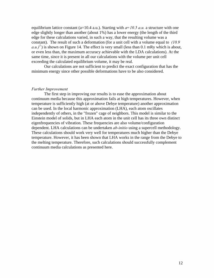
equilibrium lattice constant (a=10.4 a.u.). Starting with a=10.5 a.u. a structure with one edge slightly longer than another (about 1%) has a lower energy (the length of the third edge for these calculations varied, in such a way, that the resulting volume was a constant). The result of such a deformation (for a unit cell with a volume equal to (10.9 a.u.)3 ) is shown on Figure 14. The effect is very small (less than 0.1 mRy which is about, or even less than, the maximum accuracy achievable with the LDA calculations). At the same time, since it is present in all our calculations with the volume per unit cell exceeding the calculated equilibrium volume, it may be real.

Our calculations are not sufficient to predict the exact configuration that has the minimum energy since other possible deformations have to be also considered.

Further Improvement The first step in improving our results is to ease the approximation about

continuum media because this approximation fails at high temperatures. However, when temperature is sufficiently high (at or above Debye temperature) another approximation can be used. In the local harmonic approximation (LHA), each atom oscillates independently of others, in the "frozen" cage of neighbors. This model is similar to the Einstein model of solids, but in LHA each atom in the unit cell has its three own distinct eigenfrequencies of vibration. These frequencies are also volume/configuration dependent. LHA calculations can be undertaken ab-initio using a supercell methodology. These calculations should work very well for temperatures much higher than the Debye temperature. However, it has been shown that LHA works in the range from the Debye to the melting temperature. Therefore, such calculations should successfully complement continuum media calculations as presented here.

13

II.2. Development of New ab-initio-based Methodology A. Overview of Possible Methodologies

Because the cause of thermal expansion in solids is the elastic anharmonicity, the modeling of thermal expansion is a difficult task. There are several approximations that can be implemented to model this process. The particular choice will depend on material properties and the temperature range of interest.

We have considerable previous experience [10,11] in ab-initio-based computational modeling for predicting thermal expansion of nickel-based materials. In these calculations the technique was developed [10,12] to extract information from the ab-initio full-potential linearized muffin-tin orbitals electronic structure calculations [13,14] results, in order to generate the atomistic potentials. However this technique, was rather indirect and phenomenological. This led to limitations in easily capturing important effects providing directionality to the interatomic bonding. We have therefore developed a new technique, described below, that very directly transforms the all-electron ab initio electronic structure results of the full-potential LMTO electronic structure behavior, computationally provided in reciprocal space, to the real space representation needed for the thermal expansion modeling.

The most direct, accurate, and straightforward approach is to use direct ab-initio calculations augmented with ab-initio molecular dynamics or Monte Carlo calculations. However this approach would require an extraordinarily large amount of computations. While our FPLMTO is a highly accurate type of calculation, a direct use of it in MD/MC would exceed the capacity of modern computers.

The next possible approximation would be use of a pseudopotential. Techniques based on first-principal norm-conserving pseudopotentials [15] often can preserve the accuracy of all-electron ab-initio calculations; while at the same time they provide a significant speed-up. This is because the most difficult regions for computations, around the nuclei, are excluded from calculations. The electronic potential is relatively flat in the interstitial area where most of the interatomic bonding occurs. However, in the region immediately around the nuclei the electronic potential varies significantly. Moreover, unlike valence electrons, the deeper energy level electrons that form a core around the nuclei are insensitive to the surroundings and do not participate in bonding directly. The pseudopotential technique takes advantage of these properties of electrons in crystals. First, core level electrons are treated in the “frozen core” approximation, and their contribution to the total potential is taken from initial calculations for isolated atoms. Second, these potentials are changed around the nuclei in such a way that they are smooth inside some spherical cutoff region, but at the same time they accurately reproduce initial wave functions outside this sphere and the total charge inside it. Because the pseudopotentials are smooth by construction, the motion of the valence electrons can be calculated easily and much more quickly than in an all-electron type of calculations. At the same time, because the electron scattering properties of the nuclei are preserved, pseudopotential calculations can accurately reproduce most of the electronic properties. When the highest level core electrons significantly overlap with valence electrons, as in the case of copper, zinc and some other elements, it is possible to include nonlinear corrections [16]. There are several modern approaches for constructing pseudopotentials [e.g. based on 17-19]; however, for describing a transition metal based system, ultrasoft pseudopotentials [20] are most likely to be successful. In addition, a pseudopotential code

14

can be adapted to a parallel computer and has been successfully run on a Cray T3E and on Linux clusters. Despite all of these conveniences, the size of the supercell for such calculations is still limited to about 50 atoms. Therefore, a contribution of phonons with wavelength exceeding the size of about 15 A is neglected. While this might be a good approximation for very high temperature, these are still very demanding calculations. Thus they are basically useful as a last resort if other approximations fail to describe the thermal expansion of materials of interest.

An alternative to molecular dynamics (MD) and monte carlo (MC) simulations is to use a quasiharmonic approximation. In this approximation, while atomic oscillations (phonons) are treated harmonically, the frequencies of phonons are volume dependent. If this dependence is known, as well as the dependence of the internal energy on volume, the entire equation of state can be found and thermal properties are easily obtained through thermodynamic equations. This approximation should work well even above the Debye temperature, and it has been demonstrated that it successfully provides the melting temperature for several metals, e.g., silver [21].

The phonon dispersion at various volumes can be found without having to study various deformations of the lattice directly in a supercell. This involves use of recent developments of linear response theory based on density functional theory [22-24]. The harmonic force constants of crystals are determined by their static linear electronic response. Application of the Hellmann-Feynman theorem describes the linear variation of electronic density in response to an external periodic lattice perturbation caused by phonons. Using this approach, the phonon spectrum was accurately calculated for several transition metals, including magnetic Fe and Ni [25], and for the perovskite material KNbO3 [26].

Further speedup, and therefore larger supercells and lower cost of calculations, can be achieved by using real space (tight-binding) calculations. This approach is also suitable for parallel computers and allows treating supercells with several hundred atoms. Since this approach is based on quantum mechanics, it is still capable of providing many effects of electron gas contributions. While matrix elements of the TB Hamiltonian for elements have been recently determined [27], there are significant difficulties in finding effective interactions between different types of atoms. Below in B we describe our approach which, by a direct transformation technique, avoids such difficulties. Recent development of parallel methods of diagonalization of large matrices makes this approach very promising for the calculation of thermal properties of high-temperature alloys. When an effective TB Hamiltonian capable of describing a system in an arbitrary configuration (positions of atoms) is known, the equilibrium volume at a given temperature and pressure (NPT ensemble, where N denotes a constant number of atoms) can be found via molecular dynamics or monte carlo simulations. Alternatively, pressure as a function of temperature (NVT ensemble) can be determined if the simulations are performed with fixed volume and temperature. A volume dependence can be subsequently found using standard thermodynamic technique. Which ensemble to use depends on the system. Usually NPT simulations converge more quickly, while NVT are easier to implement.

When we compare MD and MC, it can be seen that both techniques have some benefits and disadvantages. In the case of TB they both heavily rely on a fast diagonalization of the TB Hamiltonian matrix. Generally, MD provides faster

15

convergence and can provide additional useful information about specifics of atom motions. However, MD requires calculation of forces, and therefore obtaining eigenvectors (for use in the Helmann-Feynman theorem) in addition to eigenvalues; whereas only energy calculations are necessary in MC. Modern diagonalization techniques provide much faster calculation of eigenvalues without eigenvectors, and this most likely can wipe out all benefit of faster convergence of MD. Our particular choice of a technique will be determined after initial testing.

Also, we should mention that implementing a TBMD on a parallel computer is limited to a diagonalization technique. MC, contrary to popular belief, is an inherently sequential approach, since for a proper sampling of the configuration space, steps should be taken in sequence. However recent modifications [28] allow increased parallelization of the MC algorithm itself. B. Approach Combining FP-LMTO and Tight-Binding for the Calculation of the Thermal Expansion Coefficients of Complex Materials

There are two separate parts to this approach. First, one has to extract the tight-binding parameters from the FP-LMTO results. Second, one uses these parameters to actually calculate the thermal expansion coefficient. The method we intend to use in the thermal expansion calculation is the real space method as described in the final part of Section A above. Therefore, we now describe the method used for the bridging from the full potential LMTO results to the real space (tight-binding) basis needed for the thermal expansion modeling. B.1 Extraction of TB parameters from FP-LMTO results

The ideal TB parameters would be accurate, localized, and transferable. Accuracy. The TB parameters are extracted from a FP-LMTO calculation using a single negative kappa, for a specific crystal structure (supercell). The accuracy of these TB parameters therefore can only be as good as the accuracy of the single-kappa FP-LMTO result. Calculations using the FP-LMTO method usually use 3 different kappas (e.g., see [29,30]), which can be of either sign, positive or negative. For our initial work in extracting the TB parameters, we will use a negative kappa since we want the basis function to be localized. The magnitude of the chosen kappa should not be too large since the optimal kappas (the kappa set which give the lowest total energy) typically have values around zero. Thus the choice of basis functions will be rather limited initially. However, as part of the research, as described in (3) below, we will refine the methodology to remove this limitation. Localized Basis. The spatial extent of the basis functions used is set by the value of kappa. The more negative it is, the more localized is the function. From our experience with NiAl, setting kappa = −0.2 effectively makes irrelevant the matrix elements between orbitals separated by a distance more than 7-8 lattice constants of NiAl. (While the matrix elements decay exponentially with distance, the number of neighboring orbitals within that distance goes quadratically with distance.) This means that the basis function spreads as far as about 20 Angstroms from its center. The range of the basis function also determines the size of the grid in the Brillouin zone that we need to use in the LMTO calculation. In the case of NiAl, we used a finite cubic crystal consisting of a 16 x 16 x 16 unit cell of NiAl, with periodic boundary conditions. This means we have to calculate the

16

matrix elements in momentum space, H(k) and S(k) corresponding to the Hamiltonian and overlap matrices, in the Brillouin zone with 16 x 16 x 16 points. Using symmetry, for NiAl this number was reduced to 165 inequivalent k points in the irreducible region. The dimension of the matrix for NiAl was 18 (9 spd orbitals for each atom, and 2 atoms/unit cell). Transferability. In this approach, the TB parameters are obtained from direct Fourier transform of the matrix elements in the momentum space for a specific structure and specific lattice constant. For relatively small changes in the lattice constant (keeping the same structure), as are pertinent to the thermal expansion, the parameters between orbitals located on different atoms are expected to be obtainable from smooth extrapolation/interpolation from the parameters for the starting lattice constant. The parameters that may change significantly are the onsite parameters, which depend on the onsite electron density. To make a usable look-up table, good for variable lattice constant in the same structure, one may therefore perform several runs with different lattice constants and obtain a fitting function of the onsite parameter as a function of lattice constant, for each orbital in each atom. We will investigate the quality this provides for the calculation of the bulk modulus. To deal with the transferability of the parameters between different structures, we will calculate the TB parameters using as close a structure as possible to the structure for which the TB parameters are to be used. Comparison with other approaches. The first proposal to obtain directly the TB parameters from muffin-tin based LDA methods was by Andersen and Jepsen in 1984. In their method they used the LMTO method within the atomic sphere approximation (ASA). In LMTO-ASA, the parameter kappa is set to zero, and the muffin-tin tails decay in a power law fashion with distance. Furthermore, in the ASA the interstitial region is completely neglected. To transform their long-ranged basis function to an exponentially-decaying basis, they used an additional constant: the screening parameter. They stated that the resulting TB parameters are very localized (vanish beyond 2-3 lattice constant) and highly transferable, within the ASA. The introduction of the screening parameter in their method is possible because the interstitial region is neglected in the ASA. The full-potential methods, however, treats the interstitial region as well as the muffin-tin region. For dynamic applications, one may use the FP-LMTO output as input in fitting approaches, as we have done previously [10-12], or as more recently has been done by the Naval Research Laboratory group for their tight binding methodology [27]. B.2 Modeling of the thermal expansion behavior

As stated above, we plan to use the real space methodology described in the final part of Section A. However, as resources and time allow, we will examine the possibilities offered by quasiharmonic and pseudopotential calculations.

B.3 Possible routes to improving the quality of the TB parameters

As discussed in (1) above, in our technique, at present the TB parameters are obtained from direct Fourier transform of the LMTO result (in k-space) using a single negative kappa. This gives a minimal set of basis function (9 spd orbitals for each atom). The limitation in this approach is that the most accurate result (within LDA-FPLMTO) is obtained typically with 3 kappas, which can be of either sign. One can perform the same direct Fourier transform on this result also, but this is not very practical since one is then

17

dealing with 27 basis functions for each atom. Furthermore the physical interpretation of these multiple orbitals in each atom will not be as straightforward as in the single-kappa case. What is desirable is a minimal set of basis functions that reproduces the physically relevant bands of an accurate LMTO result, i.e., the bands below and slightly above the Fermi level,. Each basis function would preferably also have a definite angular momentum symmetry (s, p, or d state, but not a mixture of two or more angular momenta). We plan to investigate two possible ways, described immediately below, to carry out the desired improvement in quality of the TB parameters.

Fitting the 3-kappa LMTO result. In this approach, we use the TB parameters from the single-kappa result as a starting set for fitting the 3-kappa result. The computational procedure is rather straightforward: parametrize the TB parameters using analytical functions and minimize the deviation of the fitting functions from the actual bands. The parameters, however, become semi-empirical---instead of first principle---and there is no a priori way to assess their accuracy. Projection Method. In this approach one starts with the ab-initio LMTO result with 3 kappas and extracts the states with the lowest energy by projecting out the higher energy states. The limitation of this approach is that the states may not have a definite angular momentum, which may give some problems related to its interpretation. However, a symmetry-based transformation may overcome this difficulty, i.e., something like the Lowdin orthogonalization where one transforms a non-orthogonal basis set into an orthogonal one which has the same symmetry.

Currently, the computational modeling methodoligies discussed above are being applied to thermal expansion calculations of iron aluminides and the results will be reported soon.

18

REFERENCES

1. B.S.-J. Kang and B. Cooper, “Thermal Expansion Modeling and Fracture Behavior of Iron Aluminides,” Proceedings of the Thirteenth Fossil Energy Materials Conference, Knoxville, May 1999.

2. Johnson, H. H., "Hydrogen Embrittlement and Stress Corrosion Cracking" (proc.Troiano Festschrift Symposium, Case Western Reserve University, June 1-3, 1980), p. 3 (edited by R. Gibala and R. F. Hehemann ), ASM, Ohio, 1984.

3. Liu, H. W., "Stress-Corrosion Cracking and the Interaction Between Crack-Tip Stress Field and Solute Atoms," Transactions of the ASME: Journal of Basic Engineering, vol. 92, pp. 633-638, (1970).

4. P.Sofronis,R.M.McMeeking, "Numerical Analysis of Hydrogen Transport Near a Blunting Crack Tip," Journal of Mechanics and Physics of Solids,Vol. 37,No.3,pp. 317-350, (1989).

5.. W.Jones, N.H.March, "Theoretical Solid State Physics", Wiley, (London, N.Y., 1973) Ch. 3.

6. C.L.Fu and M.H.Yoo, Acta. Metal. Mater 40, 703 (1992)

7. C.L.Fu and X.Wang, Philos.Mag. Lett. 80 683, (2000)

8. N.W.Ashcroft and N.D.Mermin Solid State Physics. (Holt, Reinhart, and Winston, New York, 1976).

9. M.Mehl, B.M.Klein, and D.A.Papaconstantopoulos "First Principles Calculations of Elastic Poroperties of Metals" in Intermetalic Compounds: Principles and Practice, Vol 1., ed. J.H.Westbrook and R.L.Fleischer", Wiley and Sons, (London 1995) Ch. 9.

10. J. Mei, Y.G. Hao, S.P. Lim, and F.L. Van Scoy, “New Technique for Ab Initio Atomistic Potentials and Application to Thermal Expansion of Ni/Cr Alloys”, pp 15-20, Materials Research Society Symposium Proceedings, Vol. 291 Materials Theory and Modelling (eds. J. Broughton, P. Bristowe, and J. Newsam, Materials Res. Soc., Pittsburgh, 1993).

11. J. Mei, Y.G. Hao, and F.L. Van Scoy, “Molecular Dynamics Modeling Using Ab Initio Interatomic Potentials for Thermal Properties of Ni-Rich Alloys”, pp 165-174 in Alloy Modeling and Design (eds G.M. Stocks and P.E.A. Turchi, TMS Publishing, Warrendale, PA, 1994).

12. J.Mei and S.P. Lim, “Many-Body Atomistic Model Potential for Intermetallic Compounds and Alloys and Its Application to NiAl”, Phys. Rev. B 54, 178 (1996).

19

13. D.L. Price, B.R. Cooper, and J.M. Wills, Phys. Rev. B 46, 11,368 (1992).

14. D.L. Price, B.R. Cooper, and J.M. Wills, Phys. Rev. B 48, 15,301 (1993).

15. D.R.Hamann, M.Schlüter, and C.Chiang. Phys.Rev.Lett. 43 1494 (1979).

16. S.G.Louie,S.Froyen, M.L.Cohen, Phys.Rev.B 26 1738 (1982).

17. D.R.Hamann, Phys. Rev. B 40 2980 (1989).

18. H.Troullier,J.L.Martins, Phys.Rev.B. 43 1993 (1991).

19. L.Kleinman, D.M.Bylander Phys.Rev.Lett. 48 1425 (1982).

20. D.Vanderbilt, Phys.Rev.B (1991) 41, 7892 (1991).

21. J.Xie, S. de Gironcoli, S.Baroni, and M.Scheffler Phys.Rev.B. 59 965 (1999).

22. S.Baroni, P.Giannozzi, and A.Testa Phys.Rev.Lett. 58, 1861 (1987), P.Giannozzi, S. de Gironcoli, P.Pavone, and S.Baroni Phys.Rev.B 43 7231 (1991).

23. R.Yu and H.Krakauer, Phys.Rev.B. 49 4467 (1994).

24. A.Dal Corso, A.Pasquarello, and A.Baldereschi, Phys.Rev.B. 56 R11 369 (1997).

25. A.Dal Corso and S. de Gironcoli Phys.Rev.B. 62 273 (2000).

26. R.Yu and H.Krakauer, Phys.Rev.B. 74 4067 (1995).

27. M.J.Mehl and D.A.Papaconstantopoulos, Phys.Rev.B 54 4519 (1996)

28. K.Esselink, L.D.J.C.Loyens, and B.Smit, Phys.Rev.E 51 1560, (1995)

29. L.Muratov, B.R.Cooper and J.M. Wills "Ab-Initio-Based Calculations of Vacancy Formation and Clustering Energies Including Lattice Relaxation in Fe3Al", MRS Symposium Proceedings Series (1999).

30. L.Muratov, S.Little, Y.Yang, B.R.Cooper, T.H.Myers, Phys.Rev.B. 64 035206 (2001)

31. H. Choe, D. Chen, J.H. Sceneibel and R.O. Rithchie, “Fracture and Fatigue Growth Behavior in Mo-12Si-8.5B Intermetallics at ambient and Elevated Teperature,” 2000 TMS Procedings.

Iron Aluminide

Specimen Structure Condition

Initial Fracture Mode

Environment Initial K

MPa m

Lasting Time

86-1 B2 mixed Air 36.9 7 min FA-186

86-10 DO3 mixed Air 25 28.3

94 minc 1 min

89-2 B2 intergranular Air 17.36 7 min FA-189

89-7 DO3 intergranular Air 17.36 3 min

Table1. Test matrix for the specimens studied

Alloy Total Area of

Submodel (mm2)

Area of Grain Boundaries

(mm2)

Area Fraction of GB

E GB

(MPa)

E Global

(MPa)

E matrix new

(MPa)

FA-186 1.5054 0.064 4.25% 0.564E+5 1.41E+5 1.447E+5 FA-189 0.62352 0.05 8% 0.987E+5 1.41E+5 1.443E+5

Table 2. Material properties

Stress Intensity

Factor,K

Failure Strain

Environment Fracture behavior FA 186

Fracture behavior FA 189

Vacuum

Slow and straight Stopped after 0.6mm

Very slow, blunting effect Stopped after 0.51mm

4%

Air

Very slow and straight, Stopped after 0.63 mm

Straight crack growth, after 0.4 mm it changed to multiple cracking

Vacuum (5%)

Slow and straight Stopped after 0.376mm

Stopped immediately after 0.0325 mm Almost no crack growth

K=17.3MPa√√m

6%

Air

No growth Straight slow crack extension to failure

Vacuum

Wide spread micro-cracks; relatively fast and stopped after 1.08 mm

4%

Air

Wide spread initial micro-cracks; more pronounced blunting effect, expanding damage zone growth

Vacuum

Slow and straight, blunting effect, stopped after 0.89mm

Straight crack growth; stopped after 0.56 mm

K=36.9MPa√√m

6%

Air

Less initial micro cracks (comparing to 4%) and less initial crack tip blunting

Table 3. Finite element simulation matrix

Figure 2. Fine mesh at crack tip Region (submodels)

0.2mm

Figure 1. Global model

Initial crack tip 5 mm

Figure 3. Superposed contour plots of principal strains of global model and submodel (a) FA 186 and (b) FA 189

Initial crack tip

E new submodel

Current crack tip

Initial crack tip

E new

Current crack tip

E global

Figure 4. Submodel and corresponding adjusted global model

Hydrogen diffusion zone, step Principal strain distribution, step 1, crack growth

Principal strain distribution, step 9,crack growth

Hydrogen diffusion zone, step

Hydrogen diffusion zone, step Principal strain distribution, step

Hydrogen diffusion zone, step Principal strain distribution, step 33 (stopped)

Figure 5. Hydrogen diffusion zones and principal strain distributions for FA-186, Air, √

Hydrogen diffusion zone, step 1


Principal strain distribution, step 1, crack growth

Principal strain distribution, step 2,crack growth

Hydrogen diffusion zone, step 4 Principal strain distribution, step 4,crack growth

Hydrogen diffusion zone, step 6 Principal strain distribution, step 6,crack growth

Figure 6. Hydrogen diffusion zones and principal strain distributions for FA-186, Air, KI=36.9MPa√m

Hydrogen diffusion zone, step 1 Principal strain distribution, crack growth, step1

Hydrogen diffusion zone, step 16 Principal strain distribution, crack growth, step 16

Principal strain distribution, crack growth, step 37


Principal strain distribution, crack growth, Hydrogen diffusion zone, step 48

Figure 7. Hydrogen Diffusion zones and principal strain distributions for FA-189, Air,KI=17.36MPa√m

Principal strain distribution, step 1







Principal strain distribution, step 28 (stopped) Figure 8. Principal strain distribution for FA186, KI=36.9MPa√m, Vacuum

Initial principal strain distribution Principal strain distribution, step 5 (stopped)

Figure 9. Principal strain distribution for FA189, KI=17.36MPa√m, Vacuum



Figure 10. Principal strain distribution for FA189, KI=36.9MPa√m, Vacuum




Principal strain distribution, step 63 (stopped)

Figure 11

Figure 12

Figure 13

Figure 14

evaluation of the intrinsic and extrinsic fracture

Documents