Contaduría y Administración 62 (2017) 1361–1376

Available online at

www.cya.unam.mx/index.php/cya

Evaluation of the effect of investor psychology on anartificial stock market through its degree of efficiency

Evaluación del efecto de la psicología del inversionista en un mercadobursátil artificial mediante su grado de eficiencia

Juan Benjamin Duarte Duarte, Leonardo Hernán Talero Sarmiento,Katherine Julieth Sierra JuárezUniversidad Industrial de Santander, Colombia

Received 5 January 2016; accepted 30 March 2016Available online 5 September 2017

Abstract

The main objective of this article is to develop a Cellular Automaton Model in which more than onetype of stockbroker interact, and where the use and exchange of information between investors describe thecomplexity measured through the estimation of the Hurst exponent. This exponent represents an efficient orrandom market when it has a value equal to 0.5. Thanks to the various proposals, it can be determined in thisinvestigation that a rational component must exist in the simulator in order to generate an efficient behavior.© 2017 Universidad Nacional Autónoma de México, Facultad de Contaduría y Administración. This is anopen access article under the CC BY-NC-ND license (http://creativecommons.org/licenses/by-nc-nd/4.0/).

JEL classification: G140; G170; G190Keywords: Cellular automaton; Complexity; Hurst exponent; Investor psychology

Resumen

El objetivo principal de este artículo es desarrollar un modelo autómata celular en el que interactúen másde un tipo de agentes bursátiles, donde el uso y el intercambio de información entre los inversores describenla complejidad medida a través de la estimación del coeficiente de Hurst, que representa un mercado eficienteo aleatorio al tener un valor igual a 0.5. Gracias a las variantes propuestas en esta investigación se puede

E-mail address: jbduarted@hotmail.com (J.B. Duarte Duarte).Peer Review under the responsibility of Universidad Nacional Autónoma de México.

http://dx.doi.org/10.1016/j.cya.2017.06.0140186-1042/© 2017 Universidad Nacional Autónoma de México, Facultad de Contaduría y Administración. This is anopen access article under the CC BY-NC-ND license (http://creativecommons.org/licenses/by-nc-nd/4.0/).

1362 J.B. Duarte Duarte et al. / Contaduría y Administración 62 (2017) 1361–1376

determinar que debe existir un componente racional en el simulador con el fin de generar un comportamientoeficiente.© 2017 Universidad Nacional Autónoma de México, Facultad de Contaduría y Administración. Este es unartículo Open Access bajo la licencia CC BY-NC-ND (http://creativecommons.org/licenses/by-nc-nd/4.0/).

Códigos JEL: G140; G170; G190Palabras clave: Autómata celular; Complejidad; Exponente de Hurst; Psicología del inversionista

Introduction

The capacity to find patterns and generate predictions is a natural behavior that has accompaniedhumanity since its origins, when the first people contemplated the universe in search of guidanceand answers. Since ancient times and even up to this day, the increase in the level of certainty hasconferred onto mankind a degree of satisfaction and advantage in their surroundings. Similarly, inthe field of finances, the ability to decrease uncertainty and to find non-slanted patterns translatesinto an advantage at the time of investing, increasing the wealth of the investor.

Within the history of the stock market, different studies have been carried out with thepurpose of understanding the behavior of the assets, going from deterministic to probabilisticapproaches. However, it was not until the Efficient Market Hypothesis (EMH) proposed by Fama(1970)—which has endured for decades as a pillar of classic or rational finances—that a concep-tual base was established, which provided evidence on the inability to take advantage in a marketthat provides the same opportunities to all of its agents. However, there is evidence that indicatesthat this hypothesis does not manage to explain the real behavior of the stock market.

With the objective of understanding the behavior of the stock market, Mandelbrot (1972)structures the Fractal Market Hypothesis (HMF), which contrasts with the EMH, as it proposesa memory or tendency level to replicate a behavior in the series of prices. This hypothesis wasstudied by Peter (1994) through a rescaled range analysis to explain the volatility of the realmarket and the efficiency of the same. On the other hand, a new financial study theory focusedon the behavior of the investor and not on the information of the market is proposed by Shiller(2003) in the Theory of Behavioral Finance (TBF), which contrasts with the EMH.

Due to the different hypotheses used to explain the behavior of the series of prices, and in orderto analyze the statistical behavior of the same, algorithms emerge in the so-called computationalfinances (Lebaron, 2006). These programs not only study historical behavior, but also generatenew series that emulate a real behavior. Using this methodology, Fan, Ying, Wang, and Wei (2009)propose a Cellular Automaton Model (CAM) to study the flow of information and the manner inwhich the agents interact from the perspective of a behavioral market with fractal behavior.

The objective of this investigation is to evaluate the influence of investor behavior on an artificialstock market focused on the flow of information and the capability to imitate, anti-imitate or tobe indifferent to the environment; said behavior is reflected on the theoretical efficiency of themarket. For this, we depart from the CAM and generate scenarios or variables in which behavioralagents interact, changing the dynamic of supply and demand. Subsequently a CAM with rationalagents is modeled by adapting Alexander’s filters, as well as a mixed CAM in which the agentsare affected by the information in the market and the buying, retention or sale position of theirneighbors.

J.B. Duarte Duarte et al. / Contaduría y Administración 62 (2017) 1361–1376 1363

This article is structured in the following manner: Second section—general review of thecomplexity of the market, followed by an analysis of publications related to complex systems andthe Cellular Automaton Model. Third section—explanation of the technique applied to measurethe memory in the series of data and the general points used to build the variables of the model.Fourth section—description of the considerations for each simulation. Fifth section—discussionof the results obtained. Finally, Conclusions and Appendixes sections.

Review of the literature

Review of the complexity of the market

At the end of the 1960s, Fama (1965, 1970) structured the efficient market hypothesis, study-ing the random behavior of the price in different assets through the probabilistic tendency of itsprofitability, thus defining five characteristics that were jointly present in the markets: magni-tude, depth, transparency, freedom, and flexibility. This hypothesis was contrasted by Mandelbrot(1972), who discourses on this, and who discovered that a historic financer retains a short-termmemory, which possesses fractal characteristics and, therefore, must be studied through non-linearmethodologies. Peter (1994) wrote a book in which he analyzed the behavior of the series of prices,applying a regression method through the estimation of the Hurst exponent, to evidence the fractalcharacteristics of said series and to find whether these were random, persistent or anti-persistent.

Due to different discrepancies between the theory and reality in the financial series, Bulkleyand Harris (1997) study the long-term returns in the market of New York (1982–1990), findingthat the volatility in the prices of the Stock Market is related to the over- and under-valuationof the expected gains. Wermers (1999) analyze the behavior of the same market for a differentperiod (1975–1995), finding a tendency to act together, thus evidencing the herd behavior ofthe investors. On the other hand, Chang, Cheng and Khorana (2000) gathered financial datain the United States (1963–1997), Hong Kong (1981–1995), Japan (1976–1995), South Korea(1978–1995) and Taiwan (1976–1995), and found the same characteristics in the Stock Market,thus concluding that these do not depend on the high or low capitalization of assets.

These anomalies in the expected returns and the behavior of the prices allowed Grinblatt andKeloharju (2000) to carry out a study in Finland to relate the error in valuation to the manner inwhich the investors make decisions. A category resulting from this investigation are: the ‘momen-tary agents’, who consider the historical behavior of the prices at the time of selecting; and theircounterpart, the domestic investors, who base their decisions on the recent price change. Griffin,Harris, and Topaloglu (2003), based on the work by Wermers and Grinblatt, carry out a studythat links the yields of the assets to the assets of the investors, finding that there are significantdifferences in the way that companies and people commercialize the same assets.

Fromlet (2001) compiles the investigations concerning the behavior of the investors and theclassification of the same, presenting the fundaments that go into behavioral finances: heuris-tics for the processing of information, variable available information, filtering or preference ofnews, information interpretation, the psychology of transmitted messages, expectations, relevance,overconfidence, illusion of control, the disposition effect, home bias, and the herd effect.

Behavioral finances are consolidated as a variant of classical finances by incorporating thebehavior of the agents in the behavior of their investments. Shiller (2003) conducts an investigationbased on the volatility of the 1980s using the Standard & Poor’s 500 (S&P500) index, andconcludes that the changes in the series do not correspond to the behavior of a distinctly rational

1364 J.B. Duarte Duarte et al. / Contaduría y Administración 62 (2017) 1361–1376

market. Furthermore, he countered the assumptions of the EMH, suggesting that investigationson finances must take into consideration the weakness of this hypothesis.

For his part, Lo (2005) gathered studies on the behavior of the assets and the way in whichagents invest, relating factors such as: the number of competitors in the Stock Market, the sizeof the opportunities (available benefits) and the adaptive capacity of the participants, findingthat said factors relate to the degree of the market efficiency. Thus, he proposed the AdaptiveMarket Hypothesis (AMH), which Tseng (2006) would later integrate with the EMH, using theconcept of limited rationality, behavioral finances and neurofinances to analyze the volatilityof the indices: S&P500, Dow Jones Industrial Average (DJIA), and the National Association ofSecurities Dealers Automated Quotation (NASDAQ) (1971–2005), and concluding that the AMHmanages to integrate the psychosocial aspects of the investors along with the concept of perfectcompetition and market equilibrium.

García (2013) takes up Shiller’s work, highlighting the complexity of the market by consideringtwo aspects in particular for the financial decision-making process: overconfidence, and limitedcognitive capabilities.

Review of complex systems

Gardner (1970) creates the bases for the complex systems and Cellular Automaton Models bydisclosing John Conway’s Game of Life. However, due to the structure of said model, a bias wasgenerated in the results. Therefore, Ashby (1987) differentiated the modeler of the machine andthe environment through stochastic components that act as inputs, allowing the change in statusor transformation.

For his part, Peter (1994) studies the stock market based on a complex system, in which infor-mation flows in the stock market and the agents receive it by changing position; this, in the contextof a chaotic market. For his analysis, he reviews the fractal properties through the scaled rangeof the data. Complex systems as multiple relations spaces are addressed in a multidisciplinarymanner by Tarride (1995), who incorporates fields of knowledge such as information technology,psychology and mathematics, among others, when presenting the trajectory and vision of themodeling of reality through complex systems.

Subsequently, having studied the behavior of the simulated financial series, Lebaron (2006)develops algorithms to represent the stock market through price trackers. Finally, the CellularAutomaton Model is built by Fan et al. (2009), who bring back the bases of Conway’s work andapply them to an artificial market in order to study the manner in which the agents (machines)receive the information and how said information causes the change of position (transformed).

Methodology

Hurst exponent

The Rescaled Range Analysis focuses on the study of the fractal tendency or memory of aseries and its properties across time, thus relating through the value of the Hurst exponent to thecomplexity or efficiency of a market. This is determined by calculating its variability from therange of the series and its degree of deviation.

Considering that we depart from an {Mt} series with a value between 1 ≤ t ≤ T (All valuesin this series are produced by the CAM) to be studied from the perspective of complexity, it is

J.B. Duarte Duarte et al. / Contaduría y Administración 62 (2017) 1361–1376 1365

necessary to work with the yields of the same. Subsequently, a new series of X time is generated,which relates to the original data according to its logarithmic smoothing.

Xi = ln

(Mi+1

Mi

), i = 1, 2, 3, . . ., N (1)

This period of X time is divided into A contiguous subperiods with an n longitude, so thatA ∗ n = N. Each of the I subperiods or subgroups are named, with a = 1, 2, 3, ..., A. Each elementin I is labeled Xk, a, so that t = 1, 2, 3, ..., n. For each Ia subperiod of an n longitude, the averagevalue is defined by the following expression:

〈X〉N = 1

2

N∑t=1

Xt, a (2)

The average Xt is the representative value of the series of data; however, it does not indicatewhich variable can manage to become said sequence. Therefore, a relation between each valueand the difference with its median is calculated.

X(i, N) =i∑

u=1

[Xu,a − N] (3)

with the average value and the difference between each X(i, N)y < X > N element, the standarddeviation of the sample is estimated for each Ia subperiod.

S(N) =√

1

2

N∑t=1

(Xt,a − 〈X〉N)2 (4)

Thus, the first element to calculate the Rescaled range is obtained. The second element is therange of the series of time, denominated R(N). This value is given between the maximum andminimum values of the series.

R(N) =(

max1≤i≤N

X(i,a) − min X(i,a)1≤i≤N

)(5)

The Rescaled range function F(N) is defined through the relation between the magnitude ofvalues of a series of time and the variability of the same for each subperiod.

F (N) = R(N)

S(N)(6)

In this manner, a unit of measure that scales the range by considering each standard deviation isobtained. This corresponds to a Brownian behavior, where said rescaled function is proportional to√

n for a series of time in which its values are not correlated with one another. Once all the F (N)aare obtained, they are then averaged in order to obtain an estimation of the scaled variability forthe series of time.

F (N) = 1

A

A∑a=1

F (N), a (7)

1366 J.B. Duarte Duarte et al. / Contaduría y Administración 62 (2017) 1361–1376

The rescaled range function is proportional to the Hurstian T root:

F (N) ∝ a ∗ TH (8)

Said ratio can be deduced graphically through the behavior of the series for an Ln T axiscompared to the Ln F (T ).

When the estimated value of the Hurst exponent approaches 1 in the interval (0.5,1] the seriesis considered to be persistent; this means that if the values are on the rise, it is most probable that itwill continue in this manner. Conversely, in the interval [0,0.5), if it is closer to zero, its behaviorwill be anti-persistent and if at any moment it goes on the rise, it is likely that it will then beginto decrease; if H = 0.5, it is then considered to be a random series.

Cellular Automaton Model

The development of the code was based on the results of the investigation carried out by Wei,Ying, Fan and Wang in (2009). The basic assumptions are the following:

A CAM represents a stock market. Each location in the grid of the model references a stockbro-ker in the financial market. The state of the space in the grid is consistent with that of the people.Said state varies and is represented with S(i, j)(t), which prevents the behavioral investment ofthe people in site (i,j) in time t. Three values can be chosen for this state: Sb represents the stateof purchase, Sh represents the state of retention, and Ss represents the state of the sale:

S(i, j)(t) ∈ {Sb, Sh, Ss} (9)

Rules of evolution: generally, the state changes to give way to a new state which shall bedetermined by its very origin, its neighbors, the previous moment, and the control of variableswhich can be formulated as follows:

S(i, j)(t + 1) = F (S(i, j)(t), S(i, j)(t); G) (10)

where:

S(i, j)L(t) =

⎧⎪⎨⎪⎩

S(i − 1, j − 1)(t) S(i − 1, j)(t) S(i − 1, j + 1)(t)

S(i, j − 1)(t) S(i, j + 1)(t)

S(i + 1, j − 1)(t) S(i + 1, j)(t) S(i + 1, j + 1)(t)

⎫⎪⎬⎪⎭ (11)

Represents the state of the neighbors in their respective locations (only the neighborhood foreach agent in the (i,j) position is considered). G is the vector of control variables and F is the ruleof evolution of the Cellular Automaton Model. As a common rule, it is assumed that the state ina space of the grid will be affected only by the behavior of its neighbors, which possess their owninvestment preferences that are represented by R in the model.

Cellular Automaton Model for behavioral agentsThe artificial stock market focuses on the capability of an agent to imitate, anti-imitate or be

indifferent to the position of his neighbors. For the investigation, we worked with an individualtransference probability P(i, j) and, according to the original model by Fan et al. (2009), theinteraction is studied without considering the market information or Mf. The general matrix ofposition transference, based on the state of the economy and the individual tendency to replicateor not, is evidenced in Table 1.

J.B. Duarte Duarte et al. / Contaduría y Administración 62 (2017) 1361–1376 1367

Table 1Position transference matrix for a behavioral agent.

Macro factors Neighborhood position Transference of Probabilities

Buy Retain Sell

Positive information Buy (P+Mf) (1−P−Mf)*0.5 (1−P−Mf)*0.5Retain (1−P)*(0.5+0.5*Mf) P (1−P)*(0.5−0.5*Mf)Sell (1−P)*(0.5+0.5*Mf) (1−P)*(0.5−0.5*Mf) P

Negative information Buy P (1−P)*(0.5−0.5*Mf) (1−P)*(0.5+0.5*Mf)Retain (1−P)*(0.5−0.5*Mf) P (1−P)*(0.5+0.5*Mf)Sell (1−P−Mf)*0.5 (1−P−Mf)*0.5 (P+Mf)

Source: Elaborated by the authors based on the effect of investor psychology on the complexity of the stock market: ananalysis based on the Cellular Automaton Model, 2009.P is the probability of transference in the market, originally defined as a uniform probabilistic variable with a domainbetween 0 and 1. Mf is the economic Macrofactor or the general state of the economy defined daily. However, for thevalidation of the model, and for the study of the flow of information, it is ignored, giving it a value equal to zero.

Cellular Automaton Model for rational agentsFor the construction of a CAM focused on rational agents, a rule of evolution must be defined.

In this case, a variant of Alexander’s filters was applied, and even though this is a technique thatdoes not apply rigorous statistical inference, it is accepted because it generates a dynamic throughthe active management of financial series (Duarte & Mascarenas, 2014).

It consists on investing and divesting during a determined period of time based on the rule ofpurchasing the asset when its price increases x% and selling it when its price falls x%. Nevertheless,since the CAM lacks a price generator, the filter is compared with a z% percentage increase ordecrease in the possible purchase.

z% = #Agents buying

#Agents buying + #Agents selling− 0.5 (12)

The change in position of a rational agent relates to the information—free and of quality. Theeconomic Macrofactor or the general state of the economy is then defined as a calculated variablebased on the dynamic of the CAM.

Mf = #Agents buying

#Agents buying + #Agents selling(13)

This Mf acts as a simile, considering that it does not represent the global economic behaviorof a region—as a real macrofactor—it does, however, help analyze the probable tendency of thechange. As the Mf is estimated for each iteration, it can be linked to the number of transactionscarried out throughout the previous day.1 When Mf ≥ 0.5 the economy is considered to be onthe rise.

The general position transference matrix, based on the state of the economy and the decisionfilter, is shown in Table 2.

1 Output variable in Bloomberg.

1368 J.B. Duarte Duarte et al. / Contaduría y Administración 62 (2017) 1361–1376

Table 2Position transference matrix for a rational agent.

Macro factors Neighborhood position Transference of probabilities

Buy Retain Sell

Positive information Buy z% ≥ f% z% < f% 0Retain z% > f% z% = f% z% < f%Sell 0 z% > f% z% ≤ f%

Negative information Buy z% ≤ f% z% > f% 0Retain z% < f% z% = f% z% > f%Sell 0 z% > f% z% ≤ f%

Source: elaborated by the authors.f% represents the value of Alexander’s filter. According to the state of the economy, the agent may or may not changeposition; however, in the case of doing so, said change will always be to the closest position.

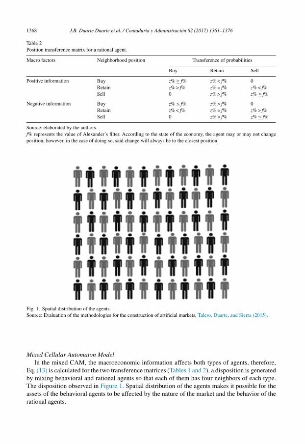
Fig. 1. Spatial distribution of the agents.Source: Evaluation of the methodologies for the construction of artificial markets, Talero, Duarte, and Sierra (2015).

Mixed Cellular Automaton ModelIn the mixed CAM, the macroeconomic information affects both types of agents, therefore,

Eq. (13) is calculated for the two transference matrices (Tables 1 and 2), a disposition is generatedby mixing behavioral and rational agents so that each of them has four neighbors of each type.The disposition observed in Figure 1. Spatial distribution of the agents makes it possible for theassets of the behavioral agents to be affected by the nature of the market and the behavior of therational agents.

J.B. Duarte Duarte et al. / Contaduría y Administración 62 (2017) 1361–1376 1369

Table 3P(i,j) distributions.

Distribution Characteristics

Uniform Continues in the [0;1] intervalNormal Median of 0.5 and standard deviation of 0.16, domain [0,1]Anti-Indifference Probability of indifference (0.5) equal to zero and symmetric, presents the form of

Fig. 2 Anti-indifference Distribution domain between [0,1]

Source: Elaborated by the authors.

Fig. 2. Anti-indifference distribution.Source: evaluation of the methodologies for the construction of artificial markets, Talero et al. (2015).

Simulation

General points

According to the CAM designed by Fan et al. (2009), a market of 50*50 cells in which theinitial position of the agents is distributed uniformly between Buying, Retaining or Selling anasset is built. The simulation is carried out for 100 iterations to demonstrate the behavior of thefinal positions of each version of the model. With regard to the analysis of the Hurst exponentand its relation to the complexity or efficiency of the stock market, only the data equivalent to theaverage longitude of the original cycle described by Fan will be considered. With L = 29. Becausea higher number of instances generate the loss of original memory (indicating the end of thenatural cycle or memory cycle).

Cellular Automaton Model for behavioral agents

The simulation is done with three types of probabilities to imitate the neighborhood (Table 3).The first is the one proposed in the original model, in which there is no predilection. In the second,the position of the agents tends to avoid being affected by its neighbors and, therefore, the behav-ioral tendency is to avoid imitating or being contrary, following a Normal distribution. Finally,the third is obliged to go in favor or against the neighborhood, though never to be indifferent, andthe probability is symmetric (Fig. 2).

1370 J.B. Duarte Duarte et al. / Contaduría y Administración 62 (2017) 1361–1376

Table 4Alexander’s filters.

f% Description

1% Permissible filter, the change of position is frequent3% Intermediate point5% Demanding filter, changes only if the information is random

Source: Elaborated by the authors.

Table 5Hurst exponent for the different P.

Distribution Hurst

Buy Retain Sell

Uniform 0.83 0.79 0.63Normal 0.58 0.66 0.58Anti-Indifference 0.77 0.84 0.78

Source: Elaborated by the authors based on MATLAB.

Cellular Automaton Model for rational agents

The simulation is done with three levels of filters to determine if, in a completely rational market,the agents adopt positions, and if the change in these represents the efficiency of the simulatedStock Market. The first filter is designed with the purpose of emulating a low decision value,which facilitates the dynamic by allowing quick changes between buying, retaining or selling.The second filter is an average point of reference for the filters used. Finally, the third representsa demanding filter, the market will only change when the stock information is reassuring. Thethree levels of filters f% are described in Table 4.

Mixed Cellular Automaton Model

An experimental 32 design is developed, with each type of agent being the{Behavioral, Rational} factor, and the variants of the models being the levels to be analyzed.N1 = {Uniform, Normal, Anti-Indifference} N2 = {1%, 3%, 5%} Three experimental repli-cas were done in order to evidence the variability of the memory or efficiency in the CellularAutomaton Model.

Results analysis

Cellular Automaton Model for behavioral agents

As initial hypothesis (H0), we have that all Hurst medians are equal, and as an alternativehypothesis (H1) we have that at least one of these is different. The resulting values from thesimulation are shown in Table 5. Hurst exponent for the different P, indicating that there arediscrepancies between the original distribution (Uniform) and those that affect the tendency toimitate or not (Fig. 3).

J.B. Duarte Duarte et al. / Contaduría y Administración 62 (2017) 1361–1376 1371

0.60

0.65

0.70

0.75

0.80

0.85

Hur

st

Anti difference NormalDistribution

Uniform

Fig. 3. Box-and-Whisker diagram according to the distribution.Source: Elaborated by the authors based on MINITAB.

Table 6Hurst exponent for different filters.

Hurst

Filter Buy Retain Sell

1% 0.88 0.87 0.933% 0.84 0.79 0.735% 0.64 0.58 0.76

Source: Elaborated by the authors based on MATLAB.

The conceptual difference between the Normal and Anti-Indifference levels is statisticallyevidenced through ANOVA. However, the uniform distribution can present a similar behavior toboth, provided that their probability of changing state is individual.

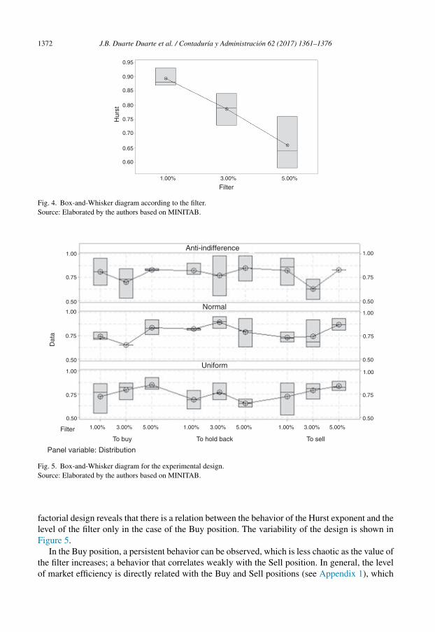
Cellular Automaton Model for rational agents

As initial hypothesis H0, we have that all Hurst medians are equal, and as H1, we have that atleast one of these is different. The estimated coefficients are shown in Table 6. Hurst exponentfor different filters indicating that there is a tendency for chaos when the value of the filter isincreased (Fig. 4).

A significant difference can be appreciated after the ANOVA between the extreme levels of thefilter factor; the value of 3%, due to being an intermediate point between these, could statisticallyestimate both.

Mixed Cellular Automaton Model

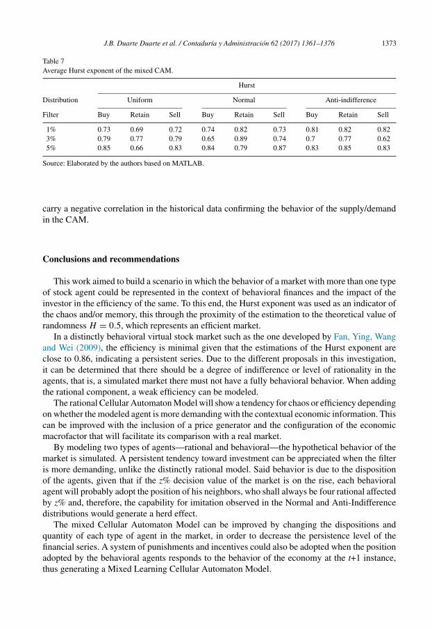
As initial hypothesis H0 for the experimental design, we have that all Hurst medians are equal;and as H1, we have that at least one of these is different. In this case, there are two factors and theinteraction between these. The Hurst exponents of the design are shown in Table 7.

By having three metrics of quality or response variables, a MANOVA is carried out, find-ing that there is a correlation between the Buy and Sell positions. On the other hand, the

1372 J.B. Duarte Duarte et al. / Contaduría y Administración 62 (2017) 1361–1376

0.95

0.90

0.85

0.75

0.70

0.60

0.65

0.80

Hur

st

1.00% 5.00%3.00%

Filter

Fig. 4. Box-and-Whisker diagram according to the filter.Source: Elaborated by the authors based on MINITAB.

Normal

Anti-indifference

Uniform

Dat

a

To buy

Filter

To hold back T o sell

Panel variable: Distribution

1.00

0.75 0.75

1.00

0.50 0.50

1.00 1.00

0.75 0.75

0.50 0.50

1.00 1.00

0.75 0.75

0.50 0.50

1.00% 3.00% 5.00% 1.00% 3.00% 5.00% 1.00% 3.00% 5.00%

Fig. 5. Box-and-Whisker diagram for the experimental design.Source: Elaborated by the authors based on MINITAB.

factorial design reveals that there is a relation between the behavior of the Hurst exponent and thelevel of the filter only in the case of the Buy position. The variability of the design is shown inFigure 5.

In the Buy position, a persistent behavior can be observed, which is less chaotic as the value ofthe filter increases; a behavior that correlates weakly with the Sell position. In general, the levelof market efficiency is directly related with the Buy and Sell positions (see Appendix 1), which

J.B. Duarte Duarte et al. / Contaduría y Administración 62 (2017) 1361–1376 1373

Table 7Average Hurst exponent of the mixed CAM.

Hurst

Distribution Uniform Normal Anti-indifference

Filter Buy Retain Sell Buy Retain Sell Buy Retain Sell

1% 0.73 0.69 0.72 0.74 0.82 0.73 0.81 0.82 0.823% 0.79 0.77 0.79 0.65 0.89 0.74 0.7 0.77 0.625% 0.85 0.66 0.83 0.84 0.79 0.87 0.83 0.85 0.83

Source: Elaborated by the authors based on MATLAB.

carry a negative correlation in the historical data confirming the behavior of the supply/demandin the CAM.

Conclusions and recommendations

This work aimed to build a scenario in which the behavior of a market with more than one typeof stock agent could be represented in the context of behavioral finances and the impact of theinvestor in the efficiency of the same. To this end, the Hurst exponent was used as an indicator ofthe chaos and/or memory, this through the proximity of the estimation to the theoretical value ofrandomness H = 0.5, which represents an efficient market.

In a distinctly behavioral virtual stock market such as the one developed by Fan, Ying, Wangand Wei (2009), the efficiency is minimal given that the estimations of the Hurst exponent areclose to 0.86, indicating a persistent series. Due to the different proposals in this investigation,it can be determined that there should be a degree of indifference or level of rationality in theagents, that is, a simulated market there must not have a fully behavioral behavior. When addingthe rational component, a weak efficiency can be modeled.

The rational Cellular Automaton Model will show a tendency for chaos or efficiency dependingon whether the modeled agent is more demanding with the contextual economic information. Thiscan be improved with the inclusion of a price generator and the configuration of the economicmacrofactor that will facilitate its comparison with a real market.

By modeling two types of agents—rational and behavioral—the hypothetical behavior of themarket is simulated. A persistent tendency toward investment can be appreciated when the filteris more demanding, unlike the distinctly rational model. Said behavior is due to the dispositionof the agents, given that if the z% decision value of the market is on the rise, each behavioralagent will probably adopt the position of his neighbors, who shall always be four rational affectedby z% and, therefore, the capability for imitation observed in the Normal and Anti-Indifferencedistributions would generate a herd effect.

The mixed Cellular Automaton Model can be improved by changing the dispositions andquantity of each type of agent in the market, in order to decrease the persistence level of thefinancial series. A system of punishments and incentives could also be adopted when the positionadopted by the behavioral agents responds to the behavior of the economy at the t+1 instance,thus generating a Mixed Learning Cellular Automaton Model.

1374 J.B. Duarte Duarte et al. / Contaduría y Administración 62 (2017) 1361–1376

Appendix 1. Effects on the Buy position during the experimental design

Average data

Anti-indifference Normal Uniform

Filter1.00%

3.00%5.00%

DistributionAnti-indifference

Normal

UniformDistribution

Filter

0.80

0.80

0.85

0.85

0.75

0.75

0.70

0.70

0.65

0.65

1.00% 3.00% 5.00%

Appendix 2. Effects on the Retain position during the experimental design

Average data

Filter

Distribution

Filter

DistributionAnti-indifference

Normal

Uniform

Normal Uniform

1.00%

3.00%

5.00%

0.9

0.8

0.7

0.9

0.8

0.7

100% 300% 500%

Anti-indifference

J.B. Duarte Duarte et al. / Contaduría y Administración 62 (2017) 1361–1376 1375

Appendix 3. Effects on the Sell position during the experimental design

Average data

Filter

Distribution

Filter

DistributionAnti-indifference

Normal

Uniform

NormalAnti-indifference Uniform

1.00%3.00%5.00%

0.85

100% 300% 500%

0.65

0.70

0.75

0.80

0.85

0.65

0.70

0.75

0.80

References

Ashby, R. (1987). Sistemas y sus medidas de Información. Tendencias en la teoría general de sistemas. Buenos Aires:Alianza Universidad.

Bulkley, G., & Harris, R. (1997). Irrational analysts’ expectations as a cause of excess volatility in stock prices. TheEconomic Journal, 107(441), 359–371. http://dx.doi.org/10.1111/j.0013-0133.1997.163.x

Chang, E., Cheng, J., & Khorana, A. (2000). An examination of herd behavior in equity markets: An internationalperspective. Journal of Banking & Finance, 24(10), 1651–1679. http://dx.doi.org/10.2139/ssrn.181872

Duarte, J., & Mascarenas, J. (2014). Comprobación de la eficiencia débil en los principales mercados financieros lati-noamericanos. Estudios Gerenciales, 30(133), 365–375. http://dx.doi.org/10.1016/j.estger.2014.05.005

Fama, E. (1965). The behavior of stock-market prices. En Journal of business, 38(1), 34–105.Fama, E. (1970). Efficient capital markets: A review of theory and empirical work. Journal of Finance, 25(2), 383–417.

http://dx.doi.org/10.2307/2325486Fan, Y., Ying, S. J., Wang, B. H., & Wei, Y. M. (2009). The effect of investor psychology on the complexity of

stock market: An analysis based on cellular automaton model. Computers & Industrial Engineering, 56(1), 63–69.http://dx.doi.org/10.1016/j.cie.2008.03.015

Fromlet, H. (2001). Behavioral finance-theory and practical application: Systematic analysis of departures from the homooeconomicus paradigm are essential for realistic financial research and analysis. En Business Economics, 3(36), 63–69.

García, M. J. (2013). Financial education and behavioral finance: New insights into the role of information in financialdecisions. Journal of Economic Surveys, 27(2), 297–315. http://dx.doi.org/10.1111/j.1467-6419.2011.00705.x

Gardner, M. (1970). MATHEMATICAL GAMES: The fantastic combinations of John Conway’s new solitaire game“life”. Scientific American, 223(4), 120–123. http://dx.doi.org/10.1038/scientificamerican1070-120

Griffin, J., Harris, J., & Topaloglu, S. (2003). The dynamics of institutional and individual trading. Journal of Finance,58(6), 2285–2320. http://dx.doi.org/10.2139/ssrn.316566

Grinblatt, M., & Keloharju, M. (2000). The investment behavior and performance of various investortypes: A study of Finland’s unique data set. Journal of Financial Economics, 55(1), 43–67.http://dx.doi.org/10.1016/s0304-405x(99)00044-6

Lebaron, B. (2006). Agent-based computational finance. In Handbook of Computational Economics. pp. 1188–1227.Iowa-Stanford: Elsevier.

Lo, A. W. (2005). Reconciling efficient markets with behavioral finance: The adaptive markets hypothesis. Journal ofInvestment Consulting, 7(2), 21–44. http://dx.doi.org/10.1016/s1574-0021(05)02024-1

1376 J.B. Duarte Duarte et al. / Contaduría y Administración 62 (2017) 1361–1376

Mandelbrot, B. (1972). Statistical methodology for nonperiodic cycles: From the covariance to R/S analysis. En Annalsof Economic and Social Measurement, 1(3), 259–290.

Peter, E. (1994). Fractal market analysis: Applying chaos theory to investment and economics. John Wiley & Sons.Shiller, R. J. (2003). From efficient markets theory to behavioral finance. The Journal of Economic Perspectives, 1(17),

83–104. http://dx.doi.org/10.1257/089533003321164967Talero, L., Duarte, J., & Sierra, K. (2015). Evaluación de las metodologías para la construcción de mercados artifi-

ciales. In Medellín, Antioquia, Colombia: IV Congreso internacional de finanzas: inversiones, Segundo encuentro deinvestigación en finanzas http://dx.doi.org/10.13140/RG.2.2.18717.10722

Tarride, M. (1995). Complexity and complex systems Histíria Ciências. Saúde – Manguinbos, II, 46–66.Tseng, K. C. (2006). Behavioral finance, bounded rationality neuro-finance, and traditional finance. Investment Manage-

ment and Financial Innovations, 3(4), 7–18.Wermers, R. (1999). Mutual fund herding and the impact on stock prices. Journal of Finance, 54(2), 581–622.

http://dx.doi.org/10.1111/0022-1082.00118