* indicates the primary contact and corresponding author

Evaluation of the Benefits of Advanced Traveler Information Systems on Supply Chain Management

Ross Beinhaker * Master of Engineering in Logistics Program

Massachusetts Institute of Technology 550 Memorial Drive, #20-C1

Cambridge, MA 02139 U.S.A Phone: 617-225-1336 Fax: 954-987-6200

Email: beinhakr@alum.mit.edu

Tomer Toledo, Ph. D. Research Associate

Intelligent Transportation Systems Program Massachusetts Institute of Technology

77 Massachusetts Ave., NE20-2008 Cambridge, MA 02139 U.S.A

Phone: 617-252-1116 Fax: 617-252-1130

Email: toledo@mit.edu

2

INTRODUCTION

Businesses are constantly searching for ways to reduce costs and increase

revenue. This is a fact of life in a world where shareholder value drives corporate

actions. In order to become more profitable, these businesses develop new processes and

techniques to create efficiency. This paper is focused on one particular new technology

that can be used to increase corporate profitability – Advanced Traveler Information

Systems (often referred to as “ATIS”).

The overall transportation industry is huge. According to the American Trucking

Association, the annual trucking market was over $600 billion in 2002. With all the

money that is spent on transportation services in the United States, any small

improvement is bound to translate into significant profit savings. In fact, better routing

has the potential to translate into reduced labor, lower fuel costs, better customer service,

improved reliability, reduced pollution, and fewer capital maintenance expenditures.

More importantly, transportation can be viewed as the key integrator of the links

in the supply chain. In many companies, this area can be vastly improved. For example,

Russell (2001) concludes that improvements in transportation related drop-off, pick-up,

and service at the customer’s location can increase overall efficiency by 10-20%. In

order to tighten the operations of the supply chain and reduce inefficiency, companies

often use fleet management software for planning and operational purposes.

The current best practices in the supply chain do not use traffic information in

transportation routing. In fact, fleet management techniques have tended to focus around

how to best assign jobs to a set of locations using a distance-based approach. This

assignment is subject to vehicle capacity and time constraints. When the problem

3

involves static and deterministic parameters, there are a number of algorithms used to

assign vehicles. Bienstock (1993) and Bramel (1996) provide a very insightful

discussion of probabilistic analyses related to many of the heuristics for static vehicle

routing problems. Powell (1995) gives an extensive survey of dynamic network and

routing models. The solutions produced by these vehicle routing algorithms will

potentially be sub-optimal if they fail to account for traffic incidents and congestion.

Advanced traveler information systems can provide users with information about

the state of the transportation network. ATIS is a sophisticated, technological

infrastructure that collects, processes, and disseminates information to end-users. For

collection, these systems utilize a wide array of sensor technologies that monitor traffic

conditions. Two primary sensoring technologies are inductive loops (buried under the

pavement) and video image processors (placed at key intersections). This “sensed”

information is then transmitted either through a wireless protocol or through a SONET

architecture to a central management center. At the management center, this information

is manipulated by software in order to be made more valuable to end-users. It is then

delivered to a user’s in-vehicle navigation system through wireless transmission.

Alternatively, the information can be provided to a central operator via the Internet.

The benefits of ATIS have been well studied. Levinson (2002) presents the value

of advanced traveler information systems for route choice. He suggests that driver

behavior will become more informed as in-vehicle navigation systems increasingly are

adopted. Wahle (2002) discusses the impact of real-time information in a two-route

scenario using agent-based simulation. He concludes that the nature of the information

influences the potential benefit of information systems. Wunderlich (1999) finds that

4

advanced traveler information systems yield time management benefits. When travel

behavior focused on travel time, Wunderlich found advanced traveler information system

users save time in terms of their total travel budget.

Table 1 presents a snapshot of the results of studies that have tried to quantify the

time savings from ATIS. These studies have differed in terms of congestion level,

congestion type, and the market share of drivers who have been provided with

information.

TABLE 1

SUMMARY OF TIME SAVED BY ATIS STUDY Author Congestion level/type Time Saved (%) Market Share (%) Levinson (2002) 95% of peak congestion 40% 50% Al-Deek et al. (1989)

Incident conditions 30-40 N/A

Peckman (1996) Field operational test 20 N/A Levinson (2002) 50% of peak congestion 20 50 Wunderlich (1995, 96, 99)

Various congestion levels 6-20 5-10

Inman et al. (1996)

Field operational test 8-11 30-50

Emmerink et al (1995)

Recurrent congestion 7 N/A

Inman et al. (1996)

Field operational test 5 10

Al-Deek et al. (1989)

Difference in system optimal and user equil.

3-4 N/A

Adler (1999) Various congestion levels 2.7 - 3.1 80-100 Emmerink et al (1996)

Recurrent congestion 1-4 100

These results illustrate the potential of ATIS to reduce travel time. However,

these studies do have several weaknesses. Many are highly theoretical and would not be

reflective of actual conditions. For example, Levinson (2002) presents a modeling

approach where driver headway is modeled by:

5

λ())ln()( RANDvH −=

where RAND () indicates a random real number between 0 and 1 and λ is the average

arrival rate. Levinson is not alone in providing a theoretical framework to operate under.

Wahle (2002) uses a simulation technique where dynamic drivers choose their route at

random. Not only are many of these models theoretical in nature, but many of them are

also simplistic. Wahle uses only two routes to simulate the decision process that travelers

will face. Levinson (2002) does no better by analyzing the case of unexpectedly reducing

capacity on one link in a network of only two parallel links. Adler and Blue (2000) do

only slightly better by examining a network that is composed of 8 nodes and 15 bi-

directional arcs.

The primary research objective of this work is to determine the impact that

differing levels of information can have on transportation practices, and therefore, in turn

on corporate profitability. This information is collected, analyzed, and disseminated

through the use of advanced traveler information systems. The end result of this work is

a quantification of this impact and conclusions related to which informational practices

should be implemented into the supply chain.

The paper that follows is different from all prior studies in the following ways:

1. To the best of the authors’ knowledge, this is the first paper that charts time

savings related to an information spectrum for commercial vehicles. The

authors present a unique classification of ATIS units according to a novel

information scheme.

2. This paper uses actual traffic data from the Los Angeles Highway System.

The results that are obtained are not absolutely theoretical in nature. In

6

addition, the network is not overly simplistic. The final results should be a

consistent reflection of the time savings that a commercial vehicle operator

would experience.

3. This paper will present recommendations to supply chain managers as to

possible best practices based on the results of the experimental study. These

recommendations will take into consideration a financial framework.

ATIS BENEFITS TO SUPPLY CHAIN OPERATIONS In the introduction, we spoke about the ability of ATIS to improve corporate

profitability. The most obvious improvement would be the time savings that result from

better routing. A decrease in the routing time can translate into a number of different

benefits. Total labor expense can be reduced if drivers do not use this time to do other

things. It is a real concern to make sure that drivers do not waste the additional time

savings. However, most drivers do not like to be stuck in traffic and so this temptation

should be minimal. In addition, a decrease in the routing time can also be translated into

fuel savings.

Capital expenditures can be decreased by using ATIS because vehicles will be out

on the roads for a shorter period of time. This should translate into lower maintenance

expenses and higher corporate profitability. In addition, general & administrative

expenses could be lowered by automating data intensive processes. As an example of

this, billing could be tied into an electronic in-vehicle unit. When a delivery is made, an

electronic bill can be sent to the customer. This could decrease account receivable days

and eliminate employees dedicated to inefficient administrative procedures.

7

While we have mentioned that time savings can be obtained by using ATIS, a

company can use this additional time to make more deliveries. This should increase the

overall revenue of a company. In addition, because the deliveries are made in a shorter

period of time, customers might be happier with their service. And an increase in

customer satisfaction might lead to more orders and higher revenue. This type of revenue

increase does not eliminate the time savings gap identified in the comments above. The

power of increasing revenue and decreasing costs simultaneously is one of the prime

attractions of implementing traffic information in the supply chain.

There are a number of external or intangible benefits that result from the

increased efficiency in routing vehicles. Driver safety can be improved. If a driver is no

longer in danger of being lost, s/he can concentrate on the road and not other factors.

This should improve the accident rate. In addition, insurance expenses might be lowered

as a result of this safety improvement.

Society as a whole should also benefit from an increase in vehicle efficiency.

Increases in pollution are creating a potential global problem. As the population grows,

this problem will become larger and larger. By reducing the amount of fuel consumed,

ITS will also decrease the amount of pollution emitted by vehicles. This is an external

benefit to all of society.

8

TABLE 2

AREAS OF POTENTIAL SAVINGS OF ATIS Area of Potential Savings Description

Labor A decrease in the time of a trip could decrease the total labor expense

Fuel A decrease in the time of a trip could decrease the total fuel consumed

Capital Expenditures A decrease in the time that vehicles are on the road could decrease maintenance expenses

General & Administrative The implementation of an ITS unit could streamline administrative procedures

Additional Revenue If additional trips are able to be made with the decrease in time, additional revenue could be obtained

Safety Driver safety improvement through routing features, lower the accident rate and decreasing insurance

Pollution A decrease in the amount of fuel consumed will lower the external pollution

THE INFORMATION SPECTRUM

Information can be divided along a number of different lines. Figure 1 highlights

two major lines of divisions: by time-period and by time-update. The first spectrum

relates to the time-period of the information that is being fed into the advanced traveler

information system. In other words, several different forms of data can be used as a base

for the mathematical computation that occurs within an in-vehicle unit. For example, the

theoretically most-restrictive type of system will be based on no information at all. A

degree above this level is a system that is run using historical information. This means

that a set of historical data that represents past traffic states could be used to guide drivers

in the present. All that need to happen is that this information is logged over time.

However, real-time sensors now offer the ability to incorporate instantaneous data into

ATIS methods. Real-time guidance has become possible through technological

advancements. Finally, at the top of this information spectrum are ATIS units that are

run using predictive information.

The second division shown in Figure 1 is the level of informational updates that

an ATIS unit can incorporate. In theory, the lowest limit is to never update at all – and is

represented by the no information tag. Of course this type of system is nonsensical and

9

for all practical purposes at least one input point needs to occur. This is the definition of

a pre-trip system. Information is entered into the system once and is not updated as time

progresses. In practice this translates into a driver being guided at an initial time point

with no successive informational updates along the way. A level above the pre-trip

update is an ATIS unit that updates a driver’s path en-route. For example, the system

could be clocked to re-compute the guidance at twenty minutes intervals. If traffic

conditions have changed, it is quite likely that the guidance will also be changed. These

adaptive systems therefore can have great practical use in real world applications.

Finally, one can think of an en-route system that is updated continuously as the highest

level of information updates. In such a system, drivers would constantly have the best

information that is available.

FIGURE 1

THE TWO DIMENSIONS OF INFORMATION

None PredictiveHistorical Instantaneous

Information along the time-period spectrum

None En-route

Information

Pre-trip

Information

Information along the time-update spectrum

The interesting phenomenon related to these two dimensions of information is

that they can be integrated to describe a specific landscape (shown in Figure 2). This

landscape provides an insightful look into the possibilities of various ATIS types.

Clearly, if there is no information input into the system – represented by the none/none

10

box – the ATIS unit will be non-rational. This type of system would generate guidance

in a random or haphazard fashion. What is more interesting to look at is the sub-matrix

that represents the feasible choices for an ATIS unit. This 3x2 matrix can be understood

by considering a diagonal movement along the x-y axis. The level of information

incorporated into the ATIS unit becomes more complex and powerful as we move from

the upper left to the lower right corner of the matrix. This movement fosters more

updates and greater “freshness” of the data being considered. In a theoretically ideal

world, an en-route/predictive ATIS unit would be the gold standard.

Before moving on, it is worthwhile to note the non-division made for historical

information. Historical information is based on a set of traffic data that has already

occurred. In this manner, it does not make sense to speak of pre-trip or en-route updates

of historical information because all information is available pre-trip. We will discuss the

historical level further in the experimental design section.

FIGURE 2

THE INFORMATION SPECTRUM MATRIX

En-route/Predictive

En-route/InstantaneousEn-route

Pre-trip/Predictive

Pre-trip/Instantaneous

Historical

Pre-trip

None/NoneNone

PredictiveInstantaneousHistoricalNone

En-route/Predictive

En-route/InstantaneousEn-route

Pre-trip/Predictive

Pre-trip/Instantaneous

Historical

Pre-trip

None/NoneNone

PredictiveInstantaneousHistoricalNone

Time-period spectrum

Tim

e-up

date

spe

ctru

m

11

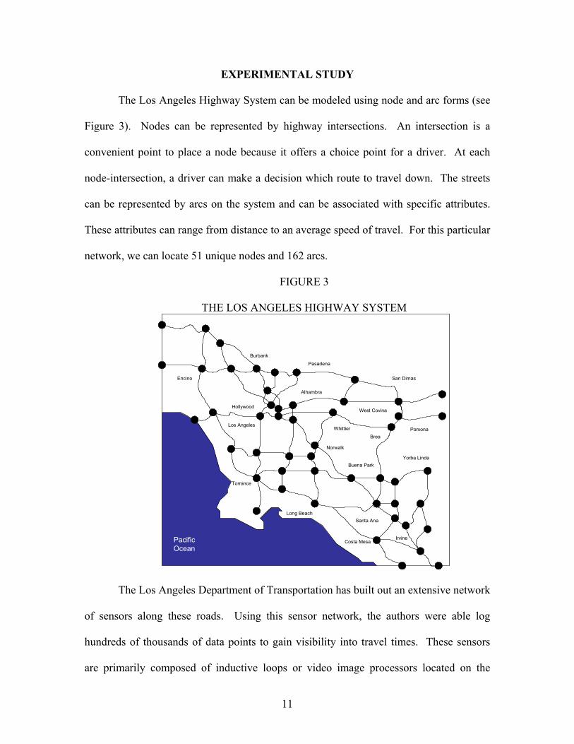
EXPERIMENTAL STUDY

The Los Angeles Highway System can be modeled using node and arc forms (see

Figure 3). Nodes can be represented by highway intersections. An intersection is a

convenient point to place a node because it offers a choice point for a driver. At each

node-intersection, a driver can make a decision which route to travel down. The streets

can be represented by arcs on the system and can be associated with specific attributes.

These attributes can range from distance to an average speed of travel. For this particular

network, we can locate 51 unique nodes and 162 arcs.

FIGURE 3

THE LOS ANGELES HIGHWAY SYSTEM

Encino

BurbankPasadena

San Dimas

Pomona

Yorba Linda

BreaWhittier

West Covina

Alhambra

Hollywood

Los Angeles

Torrance

Long Beach

Norwalk

Buena Park

Santa Ana

Costa MesaIrvinePacific

Ocean

The Los Angeles Department of Transportation has built out an extensive network

of sensors along these roads. Using this sensor network, the authors were able log

hundreds of thousands of data points to gain visibility into travel times. These sensors

are primarily composed of inductive loops or video image processors located on the

12

highways. Using a random number generator, twenty origin/destination pairs were

selected from this network for the experimental study. The only constraint that we have

imposed upon these runs is that they require at least 1 choice. This means that the traffic

run must be longer than 1 arc.

To focus on the impact of traffic, we have investigated the morning and evening

rush-hour periods over a total of five days. These five days occurred during January

2004. The rush-hour periods consisted of the 7 a.m. to 10 a.m. window in the morning

and 4 p.m. to 7 p.m. window in the evening. For simplicity, all runs were assumed to

start at the beginning of the time window.

Using the different routing policies shown in Figure 2, it possible to compute the

travel times for each origin/destination pair based on the actual parameters of the Los

Angeles Highway System. The final bridge to obtaining these results is to build a

computer model to replicate the policies. The authors chose to build these models in

C++. The primary shortest path algorithm that is used is a modified Dijkstra algorithm.

The size of the problem lent itself nicely to this type of algorithm (with a run time of

under 1 second). If the network was significantly larger, a different algorithm could have

been used.

In order to compare the policies in Figure 2, a baseline needs to be selected.

Many of the best practices in fleet management use geographical (or distance-based)

principles as a basis of computation. Today, a few companies are looking to benefit

from this type of system. They feel confident that the consistency and reproducibility of

a geographic baseline will be useful to supply chain managers. The authors chose this

level of information as a baseline comparison.

13

In Table 3, a brief description of the assumptions for each of the levels of

information is presented. These information levels correspond to the sub-matrix depicted

in Figure 2. In addition, a summary of the implementation considerations is also shown.

TABLE 3

DESCRIPTION OF EXPERIMENTAL STUDY INFORMATIONAL LEVELS Information Level Assumptions Implementation Level 0: Baseline

o The route is chosen using the shortest distance between origin/ destination

o No traffic information is considered

o Easy to implement; only need geographical database

Level 1: Historical

o The route is chosen using the shortest historical travel time between origin/destination

o The historical information used for computation is the day prior

o Fairly easy to implement o Doesn’t need to be real-

time o Doesn’t need in-vehicle

communication Level 2: Pre-trip/ Instantaneous

o The route is chosen using the pre-trip shortest travel time between origin/destination

o The travel time is calculated using real-time information

o The route is not modified as the trip progresses and traffic conditions change

o Moderately difficult implementation

o Needs to be real-time o Doesn’t need in-vehicle

communication

Level 3: En-route/ Instantaneous

o The route is chosen using the shortest travel time between origin/destination

o The travel time is calculated using real-time information

o Time updates come every five minutes

o The route is modified as the trip progresses and traffic conditions change

o Difficult implementation o Needs to be real-time o Needs in-vehicle

communication

Level 4: Predictive

o The route is chosen using the absolute shortest travel time between origin/destination

o The travel time is calculated using predictive information

o It is assumed that the agent has perfect information

o Difficult implementation o The prediction needs to be

made in real-time o Needs in-vehicle

communication

14

EXPERIMENTAL RESULTS Time Savings Analysis

Table 4 depicts the average % time savings over baseline for each day in

aggregate (both morning and afternoon). These aggregates are the average of the time

savings for each of the twenty origin/destination pairs. The average of the five days time

savings is then given in the composite column. The first conclusion to note is that there

appears to be a fairly consistent trend in the way we have laid out the information

spectrum. As we progress up the information spectrum, it appears that more and more

value can be extracted in the form of time savings. It is also important to note that Level

4 has been modeled assuming perfect information and, therefore, represents an upper

bound of the spectrum.

The notable exception to the trend is Level 1. Historical information seems to not

offer any significant time savings over the baseline. Why is this so? One possible reason

is the historical policy used for routing. The experimental results were derived by using

the previous day’s traffic information as the historical input. A more robust routing

policy would be to use a time-series analysis of several days worth of data. This would

smooth out non-recurring events.

A second conclusion to draw from Table 4 is that Level 2 and 3 seem to offer

decent time savings over the baseline. It is important to realize that all days have a

positive % time savings in each of these information levels. This implies that a high

degree of reliability can be maintained with these systems. If there were large swings of

positive and negative numbers, reliability might impede the roll-out of these types of

systems in a large-scale manner. Finally, Day 5 appears to offer the most savings for

15

both Level 2 and 3. Level 2 has a 7.23% time savings. Level 3 has a 9.18% time

savings. This suggests that these types of systems have the ability to yield large savings

on specific days. Our analysis seems to indicate that ATIS offer savings below the 15%

level over baseline. Many of the analyses presented in Table 1 that offer 40-50% time

savings are not supported by our experimental results.

TABLE 4

SUMMARY: AGGREGATE % TIME SAVINGS OVER BASELINE Day 1 Day 2 Day 3 Day 4 Day 5 Composite

Level 1Historical 3.40% -0.91% 0.41% -0.93% 1.13% 0.62%

Level 2Pre-trip, Instantaneous 1.20% 4.71% 1.85% 4.12% 7.23% 3.82%

Level 3En-route, Instantaneous 2.56% 6.87% 3.97% 7.56% 9.18% 6.03%

Level 4Predictive 4.60% 9.29% 5.25% 9.61% 11.75% 8.10% Coefficient of Variance Analysis

From a supply chain perspective, a reduction in travel time is not the only feature

that is desirable. A key concern is to eliminate extreme outliers. In other words, if there

is a great deal of variance in the travel times, companies might need to establish

excessive lead times in order to satisfy customer service thresholds. In this section, we

investigate whether ATIS units have the ability to reduce the variance in travel time

dispersion.

Table 5 presents the aggregate (both morning and afternoon) % reduction in the

coefficient of variance for each of the information levels. As can be seen in the table, all

levels of information have reduced the variance of the travel times compared to the

baseline in composite. It is also notable to highlight the fact that the trend in the

16

information spectrum appears to hold for the variance analysis as well. As we progress to

higher levels of the information spectrum, a greater % reduction in the coefficient of

variance occurs.

TABLE 5

SUMMARY: AGGREGATE % REDUCTION IN VARIANCE OVER BASELINE Level 1 Level 2 Level 3 Level 4

Pre-trip En-routeHistorical Instantaneous Instantaneous Predictive

% Reduction 7.02% 14.54% 20.07% 33.55% Sensitivity Analysis

What were to happen to the results produced by these ATIS units if this data was

erroneous? We next perform a sensitivity analysis that introduces stochastic error into

the data that we use to route corporate drivers. As an example of this situation, imagine

that due to a malfunction (caused by mechanical failure, inclement weather, etc.) a

random error component is appended to the true average speed parameter. We can label

the true speed parameter c(t) and say that the estimate of c(t) is c’(t) = c(t) + ε , where ε

is a random error term. One could logically deduce that if this random component were

large enough, it will affect the ultimate route that an ATIS unit would produce. On the

other hand, it might be the case that small random fluctuations will have no influence on

the end route.

The random error terms that we are introducing in this section will be modeled

using a Normal distribution with a mean of zero and a 5% standard deviation.

Mathematically, the random error terms can be represented as:

)_,0(~ devstdNε

17

This means that the error terms will follow a distribution that is centered on zero. As

such, given a large enough sample, the average perturbed speeds should approximate the

true speeds.

Table 6 shows the aggregate results for the sensitivity analysis. This is a

representation of the information spectrum: from Level 1 through 4. As can be seen in

the table, there is clearly a positive trend along the information spectrum. Information

Level 1 performs a little worse than the baseline. The reasons for this are equivalent to

those given in previous section.

TABLE 6

SUMMARY: AGGREGATE % TIME SAVINGS OVER BASELINE – ERROR

Day 1 Day 2 Day 3 Day 4 Day 5 CompositeLevel 1Historical 2.21% -2.00% -0.60% -2.23% 1.11% -0.30%

Level 2Pre-trip, Instantaneous 1.43% 4.57% 1.19% 4.41% 6.76% 3.67%

Level 3En-route, Instantaneous 2.28% 6.85% 3.61% 6.11% 9.19% 5.61%

Level 4Predictive 4.43% 9.21% 4.80% 9.15% 11.31% 7.78% The instantaneous information levels (Level 2 and 3) both produce positive time

savings compared to the baseline – even with the introduction of a small bit of error.

Because it is highly likely that a real-world ATIS unit would contain such error, it is

encouraging to see that the results still hold at small error levels. If the sensors can keep

there errors below a 5% standard deviation level, it is likely that advanced traveler

information systems will be able to add value to the supply chain.

ECONOMIC ANALYSIS

18

A monetary framework of the benefits in Table 2 can be derived. It is important

to note a few factors before presenting this framework. The first factor that is important

to consider is that the time savings we are evaluating are related to the baseline

(geographical information). Since most companies do not even incorporate the baseline

into their supply chain operations, the benefits we calculate should be much larger than

what is presented in this section.

We can compute the value of time savings for a fictional company called ABC

Inc. The first stage in the analysis is to calculate how much time is saved per day for one

commercial vehicle. Based on a 6 hour driving window, we can apply the % time

savings over the baseline for each of the information levels (1 through 4). We are using

the six hour period because this is the sum of the two rush-hour periods. We can make

the assumption that the vehicle is out making deliveries during this entire period.

Using the time saved per day, we can apply a value of time derived by Levinson

and Smalkowski (2002) to determine the total savings per day for one vehicle. Levinson

and Smalkowski derive a value of time for commercial operators of $49.42/hour using a

tobit model. The next stage in the analysis is to assume a fleet size for ABC Inc. As a

benchmark, UPS has more than 1,000 vehicles in its private fleet (Chandler 2003). Wal-

Mart maintains a fleet of 7,000 tractors and 35,000 trailers (Shein 2003). Continuing our

trend of being conservative, we will use a fleet of 250 vehicles. Using this fleet size, we

can calculate the total savings per year (after assuming a 300 day work year).

Looking at Table 7, we can see that ATIS can give additional benefits over the

baseline of hundreds of thousands of dollars per year. With perfect information, the

savings can get up to millions of dollars per year. We should also note that there is an

19

implementation cost for ATIS units. This cost can be significant if we are considering

above the pre-trip/ instantaneous level. The cost of implementation for an en-route

system might wipe out a year’s worth of savings. However, the pre-trip implementation

costs are most likely substantially lower than the en-route scenarios.

TABLE 7

TOTAL SAVINGS Level 1 Level 2 Level 3 Level 4

Units H P-I E-I PredValue of time $/hour $49.42 $49.42 $49.42 $49.42Hours per day hour 6.0 6.0 6.0 6.0% savings 0.6% 3.8% 6.0% 8.1%

Time savings per day hour 0.0 0.2 0.4 0.5

Total savings per day $/day $1.84 $11.33 $17.88 $24.02

Number of trucks trucks 250 250 250 250

Total savings $/day $460 $2,832 $4,470 $6,005

Days per year day 300 300 300 300

Total savings/year $/year $137,882 $849,530 $1,341,012 $1,801,359

SUPPLY CHAIN RECOMMENDATIONS

The first recommendation is the most important. The authors recommend that

supply chain professionals incorporate advanced traveler information systems into their

operations. Many businesses simply do not employ any systematic process in their intra-

routing decisions. There is a great deal of value to be had by companies that begin to

adopt this new technology. Currently, several leading companies employ fleet

management techniques that determine the order of customer/supplier pickup and

deliveries using a traveling salesman type algorithm. Only a handful of these companies

have even employed a shortest-distance based routing policy between these origin and

destinations. Drivers are left to their own perceptions to be able to find the best way to

20

get from location to location. Moreover, a traveling sales type algorithm that does not

incorporate traffic information is potentially sub-optimal.

There is additional value to be obtained from using higher levels of information.

In fact, pre-trip/instantaneous information can be a cheap alternative to improve the

baseline performance. One of the biggest differences between implementing a pre-trip

vs. en-route system is cost. In order to get an en-route system to operate, all of the driver

vehicles must have a communication device to receive modified routing instructions.

Drivers must also deal with changing their routes. This could be a taxing challenge for a

driver (leading to non-compliance). In addition, the vehicle must be equipped with a

GPS device to indicate to the ATIS unit the current location of the driver. This will add

to the cost as well. All of these factors make the implementation of an en-route system

more costly than a pre-trip system. For this reason, the en-route levels must offer a large

degree of time savings compared to a pre-trip system. As seen in the experimental

results, this was not the case. There was only a 2 percentage point increase in the en-

route/instantaneous level over the pre-trip/instantaneous level.

En-route information should not be eliminated from future consideration,

however. As technology proliferates and the cost of providing the dynamic features

described above falls, en-route information might be the best option. In fact, the authors

believe that in the future, en-route systems will prevail. The fact of the matter is that en-

route systems may perform better than pre-trip systems (as evidenced by Table 4’s

results). But the cost from moving between the pre-trip and en-route systems is currently

too great to justify the benefit. In the long-run, this cost will likely fall and the en-route

systems will hold sway.

21

The cost of prediction is extremely low. Modeling techniques can be used to

forecast the system. In today’s corporate world, forecasts are made from everything to

employee headcount to product demand. It does not make sense to not employ the same

tactics to transportation planning. Moreover, it was demonstrated in the simulation

results that prediction is likely to offer additional benefits to corporations.

One of the specific levels of information that we did not test was pre-trip/

predictive (not using perfect information). The authors believe that a pre-trip/predictive

model would have additional value over the pre-trip/instantaneous information level.

Essentially, the pre-trip/instantaneous model based all of its routing decisions on an

uncongested highway system. Since the routing decisions were made pre-trip and at pre-

rush hour levels, this model was extremely naïve. All in all, the authors believe that the

pre-trip/predictive information level is likely to offer the most benefit to corporations at a

reasonable cost for the near-term if an accurate forecast can be made.

CONCLUDING REMARKS This paper has hopefully given the reader a look into the future of the supply

chain. In particular, it is hoped that the reader now has an appreciation of how powerful

advanced traveler information systems can be. These systems are cutting-edge

technology and are rapidly expanding in presence and scope.

In the future, corporations that want to achieve higher profitability will need to

turn to new technologies like ATIS. Those companies that fail to be adopters will face a

significant competitive disadvantage. ATIS offers corporations visibility into

transportation networks in much the same way that radio frequency identification offers

visibility into inventory. It is a powerful new tool that companies should begin to adopt.

22

NOTES

Adler, Jeffrey, Victor Blue, and Tzu-Li Wu (1999), “Assessing Network and Driver Benefits from Bi-objective In-Vehicle Route Guidance,” Presented in the 78th TRB Annual Meeting. Al-Deek, Haitham and Adib Kanafani (1989), “Some Theoretical Aspects of the Benefits of En-Route Vehicle Guidance (ERVG),” UCB-ITS-PRR-89-2. American Trucking Association (2002), American Trucking Trends 2002, Alexandria, VA. Bienstock, Daniel, Julien Bramel, and David Simchi-Levi (1993), “A Probabilistic Analysis of Tour Partitioning Heuristics for the Capacitated Vehicle Routing Problem with Unsplit Demands,” Mathematics of Operations Research, 18, pp 786-802. Bramel, Julien and David Simchi-Levi (1996), “Probabilistic Analyses and Practical Algorithms for the Vehicle Routing Problem with Time Windows,” Operations Research, 44, pp 505-509. Chandler, Kevin, (2003), “UPS CNG Truck Fleet: DOE/NREL Truck Evaluation Projects,” Presentation at the NGVTF. Emmerink, Roderik, Erik Verhoef, Peter Nijkamp, and Piet Rietveld (1995), “Information in Road Networks with Multiple Origin-Destination Pairs,” TI 5-95-1198, Tinbergen Institute. Inman, Vaughan and Joseph Peters (1996), “TravTek Global Evaluation Study,” FHWA-RD-96-031, Washington, D.C. Levinson, David and Brian Smalkoski (2003), “The Value of Time for Commercial Vehicle Operators in Minnesota,” Transportation Research Board International Symposium on Road Pricing, Key Biscayne, Florida, November 20-22. Levinson, David (2002) “The Value of Advanced Traveler Information Systems for Route Choice,” Transportation Research Part C: Emerging Technologies. Vol 11. pp 75-87.

23

Peckmann, Max (1996), “STORM Stuttgart Transport Operation by Regional Management – Results on the Field – Trials and Assessment,” Intelligent Transportation: Realizing the Future Conference, Oct. 14-18. Powell, Warren, Patrick Jaillet, and Amadeo Odoni (1995), “Stochastic and Dynamic Networks and Routing,” Handbooks in Operations Research and Management Science, Vol. 8, Elsevier, Amsterdam. pp 141-296. Russell, Christopher (2001), “ROI Case for Vehicle Routing: Why You Should Invest Your Capital in the Last Leg of the Supply Chain?” ITtoolbox Supply Chain. Shein, Esther (2003), “Radio Flier: Wal-Mart Presents its Vendors with an Offer They Can’t Refuse,” CFO Magazine, November Issue, pp 37-39. Wahle, Joachim, Ana Bazzan, Franziska Kluegl, and Michael Schreckenberg (2002), “The Impact of Real-time Information in a Two-Route Scenario Using Agent-Based Simulation,” Transportation Research Part C: Emerging Technologies. Vol. 10. Issue 5-6. pp. 399-417. Wunderlich, Karl (1999), “Quantifying Reliability Benefits for Users of Advanced Traveler Information Systems (ATIS),” The MITRE Corporation. Wunderlich, Karl (1996), “An Asssessment of Pre-Trip and En-Route ATIS Benefits in a Simulated Regional Urban Network,” Intelligent Transportation: Realizing the Future Conference. Wunderlich, Karl (1995), “Congestion and Route Guidance Benefits Assessment,” The MITRE Corporation, ITS-L-131.