evaluation of the 1986 aashto overlay design...

TRANSPORTATION RESEARCH RECORD 1215 299

Evaluation of the 1986 AASHTO Overlay Design Method

HAIPING ZHOU, R. G. HICKS, AND I. J. HUDDLESTON

The 1986 AASHTO Guide for Design of Pavement Structures is currently being evaluated in Oregon for use in the design of overlays. This newly revised guide presents two nondestructive methods for determining the strength of existing pavement structures so that the remaining life of the pavement can be evaluated. In the evaluation of the AASHTO overlay design procedure, five project sites around Oregon were selected, including four flexible pavements and one rigid pavement. Deflection measurements were taken using both the Falling Weight Deflectometer and Dynaflect. Cores were also tested to aid in evaluating paving materials. Three backcalculation programs (BISDEF, ELSDEF, MODCOMP2) were used to compute the moduli of the pavements, and the results were used to perform the overlay design. These results were compared with the current ODOT procedure, which is based on tolerable maximum deflection; and considerable inconsistency was observed. Generally, the AASHTO method provided a thinner overlay than the ODOT procedure. The results of this study show that the guide has an important advantage in that pavement strength for each layer can be quantified (NDT method 1) and remaining life may be taken into account. However, further investigation is still required to verify the method of determining existing pavement strength from backcalculation programs and the remaining life of the existing pavement. Therefore, the guide should be used with caution at the present time.

Problem Statement

Currently, the Oregon Department of Transportation (ODOT) uses the California Transportation Department (Caltrans) Procedure with some modifications to design flexible overlays over distressed highway pavements (1). The Portland Cement Association (PCA) and American Association of State Highway and Transportation Officials (AASHTO) methods are employed for Portland cement overlays (2, 3). Currently, either the Dynaflect or the Falling Weight Deflectometer (FWD) are used to obtain deflections for the flexible overlay design procedure. The maximum surface deflection obtained using the FWD or Dynaflect (converted to an equivalent Benkelman beam deflection) is used in the modified Caltrans method ( 4). For Portland cement concrete overlays, the overlay thickness is determined by subtracting the new design from the

H. Zhou and R. G. Hicks, Department of Civil Engineering, Oregon State University, Corvallis 97331. I. J. Huddleston, Oregon Department of Transportation, Salem, 97310.

effective thickness of the existing pavement (PCA and AASHTO methods).

In both instances, the data generated are insufficient to define accurately the structural adequacy of the existing pavement. In addition, the current procedures do not take into account the remaining life of the existing pavement. To enable designers to make better evaluations on the remaining life of the pavement and provide for more efficient utilization of paving materials, a new overlay design method is needed. The development and use of this new procedure should assist in determining the structural capacity and remaining life.

Purpose

The purpose of this paper is to present an evaluation of the use of the 1986 AASHTO Guidelines (5) on selected projects in Oregon. This has included the following steps:

l. Selecting typical project sites for deflection measurements and materials sampling;

2. Laboratory testing materials sampled from each project; 3. Analyzing deflection basin data and developing overlay

design recommendations; 4. Discussing results; and 5. Developing appropriate conclusions and recommenda

tions.

1986 AASHTO OVERLAY DESIGN METHOD

Concept

This overlay design procedure is based on the serviceabilitytraffic and structural capacity-traffic relationships developed at the AASHTO Road Test. Determination of an overlay is accomplished by using a deficiency approach; Figure 1 illustrates seven steps that are generally involved. Of these steps, materials characterization and effective structural capacity analysis require the most effort. Two nondestructive test (NDT) methods are presented in the guide and can be used to analyze the existing pavement structure. They are (1) determination of pavement layer moduli (NDT method 1) and (2) determination of the total structural capacity (NDT method 2). Both methods rely on the use of deflection data generated from a nondestructive testing device.

300 TRANSPORTATION RESEARCH RECORD 1215

STEP 1 STEP 4

Analysis Unit ~

Effective Structural Delineation Capacity Analysis

scxefl

' ,

STEP 2 STEP 5 STEP 7 Future Overlay

Overlay Design Traffic Analysis Structural Capacity - Analysis Analysis

S:.y

• ' STEP 3 STEP 6

Materials and Remaining Life

Environmental Study ,_____ Factor Determination -

FIGURE 1 Required overlay design steps.

NDT Method 1

NDT method 1 is a technique used to determine the structural capacity of an existing pavement. This technique uses measured deflection basin data from an NDT device to backcalculate the in situ layer elastic moduli, and it is applicable to both flexible and rigid pavements. The fundamental premise of this solution is that a unique set of layer moduli exist such that the theoretically predicted deflection basin is equivalent to the measured deflection basin. To implement this technique, a computer program that backcalculates the elastic modulus for each pavement layer is necessary. The obtained moduli are related to layer coefficients using various charts given in the guide. The structural number is then determined using the equation

where ai equals the layer coefficient for each layer and hi equals the thickness of each layer above subgrade.

NDT Method 2

NDT method 'l is based upon the maximum measured deflection from the dynamic NDT equipment and, as such, does not require a computerized model to backcalculate layer moduli (EJ With NDT method 2, the maximum measured deflection is used to determine effective pavement structural number (SNxeff) from Burmister's two-layer deflection theory. For a particular pavement structure, the SNxeff value can be determined by a trial-and-error process. This is done by assuming an SN,eff and computing the deflection d0 • If the calculated d

0 does not agree with the maximum measured deflection

(temperature adjusted), a new SNxerr is assigned. The process

FR..

1s repeated until the calculated deflection matches the maximum measured deflection. A computer program has been developed to solve these equations (6).

PROJECTS EVALUATED

Project Descriptions

Fidu <lala were collected in the spring of 1987 at five project sites on existing highways in the state of Oregon. Four of the project sites were flexible pavements, and one was a rigid pavement. The age of the projects ranged from 10 to 25 years. Figure 2 shows the location of the project sites, and Figure 3 shows the typical cross sections.

For each of the project sites, data were collected on past and current traffic volumes. The new AASHTO overlay design traffic analysis suggests that two types of data be collected: the cumulative 18k ESAL repetitions until an overlay is placed and the cumulative 18k ESAL expected in the future for the overlay. However, the historic traffic is required only if the traffic method of determining remaining life is used. Table 1 includes a summary of traffic information obtained for each project.

The existing pavement conditions for the five sites varied considerably from one to the other. Two of the test sites (King's Valley Highway and Salem Parkway) did not show any signs of pavement surface distress. The Lancaster Drive site had been overlaid the previous year and, at the time its surface was tested, was in an excellent condition. The Willamina-Salem Highway site showed a considerable amount of cracking, both alligator and longitudinal. The PCC site (Wilsonville-Hubbard Highway) showed a fair amount of cracking in most slabs.

Zhou et al.

FIGURE 2 Location map of the project sites.

Pavement Deflection Measurements

Pavement surface deflections were measured at 50-ft intervals for 1,000-ft sections for each project. The measurements were taken with the KUAB Falling Weight Deflectometer (FWD) and the Dynaflect, both owned and operated by ODOT. For each site, deflection basin measurements were taken in the outer wheelpath. The FWD data were taken at three load levels and converted to a 9,000-lb load level by simple linear interpolation. The Dynaflect data were measured at a 1,000-lb cyclic load and at a frequency of 8 Hz. The Dynaflect and FWD tests were conducted at the same locations so direct comparisons could be made.

The Dynaflect employs two counter-rotating masses to apply a peak-to-peak dynamic force of 1,000 lb ( 4.4 kN) at a fixed frequency of 8 Hz. The force is applied to the pavement through the use of two steel wheels 20 in. (50.8 cm) apart, and the deflection basin is measured using five sensors. The spacing of the sensors on this equipment is 1 ft. The ODOTowned KUAB Falling Weight Deflectometer is trailer-mounted and towed by a %-ton van. The impulse force is created by dropping a set of two weights from different heights. By varying the drop height, the load at the pavement surface was

301

SALEM PARKWAY

varied from 4,900 to 11,300 lb. The two-mass system is used to create a smooth load pulse similar to that created by a moving wheel load (7, 8). Surface deflections were measured with four seismic transducers (seismometers) that are lowered automatically with the loading plate and spaced 12 in. apart. Since the FWD can apply a load pulse similar to that produced by a loaded truck, there is no need to correct the determined in situ moduli for stress sensitivity. The load configurations for both the FWD and Dynaflect are shown in Figure 4.

Deflection Results

For each analysis section, the mean and standard deviations of the maximum measured deflection were calculated. Those basins with a maximum deflection that varied by less than the mean or more than 1.5 standard deviations from the mean were discarded. Of the remaining basins, five were randomly selected for further analysis.

In Table 2, the 9,000-lb load level is for the FWD and the 1,000-lb load level, for the Dynaflect. The deflection basins for the FWD were obtained at the 9,000-lb load level by linearly interpolating between the two adjacent load levels.

a) King's Valley Highway b) Wiiiamina-Saiem Highway

c) Lancaster Drive d) Salem Parkway

12 in.

10tn.

• • 1 Otn. ~ 121

n. ,1,

--HillIJ:•1n.

1 ~ 1"i '

• • •

12 in . 12 in.

a) FWD

• 121n. I 121n. ' . ., 121n.

• •

e) Wiisonviiie-Hubbard Highway b) Dynaflect

FIGURE 3 Cross sections of pavements analyzed. FIGURE 4 Load configuration for both NDT test units.

TABLE 1 SUMMARY OF PROJECT DATA

Project

King's Valley Highway

Willamina-Sal em Highway

Cross- Section

6.0" AC 14.0" Agg. Base Subgrade


Traffic

4500 ESAL/yr 10 yr TC = 6.0 Cumulative ESAL = 5xl04

Future traffic = 33,200

Current = 173,200 ESAL/yr 10 yr TC= 9.7

Pavement Condition

Good surface condition Drainage adequate

Fair to Poor Longitudinal and alligator cracking

in all lanes

• J

Cumulative ESAL = 2xl06

Future traffic = 1,876,600 Evidence of rutting on outside lanes

Lancaster Drive

Salem Parkway

WilsonvilleHubbard Highway


4.5" AC 10.0" CTB 6.0" CTS Subgrade

7. 5" PCC 5.0" Agg . Base Subgrade

Total Accum . 15 years -40,000 ESAL/yr 20 yr Future t raffic = 1,000,000

Current = 135,000 ESAL/yr Accumulative = 420,000 ESAL 20 yr Future traffic = 3,200,000

Current = 115,000 ESAL/yr 10 yr TC= 9.1 Future traffic= 1,097,300

[18 kip EAL ' s) O.ll9

Note: TC Traffic Coefficient 9.0 -- 6 10

Surface condition very good Drainage good

Surface condition and drainage very good

Good to Poor Cracking of slab Erosion of shoulders

TABLE 2 DEFLECTION VALUES FOR THE PROJECTS EVALUATED

Sensors (xl0-3) in . Reading Load Number Equipment (lbs) 2 3 4 5

King's Valley Highway

FWD 9000 20 .9 16.1 10.6 6.31 Dynaflect 1000 1. 02 0.76 0.47 0. 27 0.16

2 FWD 9000 20 . 76 16.14 10.67 6.25 Dynaflect 1000 1. 12 0.81 0.49 0.28 0.16

3 FWD 9000 22. 17 16.79 10.52 5.72 Dynaflect 1000 1.26 0.90 0.51 0.28 0.17

4 FWD 9000 22 . 19 16 . 97 10 .47 5. 77 Dyna fleet 1000 0.95 0.74 0.47 0.29 0.17

5 FWD 9000 22.27 16.39 9.88 5. 02 Dyna fleet 1000 1. 09 0. 77 0.43 0.24 0.14

Willamina-Salem Highway FWD 9000 36.57 22.65 10.39 4.47 Dynaf lect 1000 1. 76 0.98 0.42 0.20 0 . 12

2 FWD 9000 42 .35 25.12 10.62 3.98 Dyna fleet 1000 2. 27 1.17 0.45 0.20 0.10

3 FWD 9000 43 .82 27.36 11.18 3. 69 Dyna fleet 1000 2.39 1. 09 0.37 0. 16 0. 10

4 FWD 9000 36 . 77 22.22 9.50 3.32 Dyna fleet 1000 1. 84 1. 03 0.43 0. 17 0. 08

5 FWD 9000 39 .80 24 . 70 8 .95 3.76 Dyna fleet 1000 1.90 1. 07 0.47 0. 23 0.14

Lancaster Drive

FWD 9000 26 . 17 19 .80 11.10 7. 70 Dyna fleet 1000 1. 55 1.11 0.71 0.46 0.31

2 FWD 9000 27 .30 20 .30 12 . 08 7. 23 Dyna fleet 1000 1. 65 1.16 0.72 0. 44 0.31

3 FWD 9000 26.39 21.13 12.62 7.94 Dyna fleet 1000 1.65 1. 22 0.78 0. 47 0.33

4 FWD 9000 26 . 06 19.86 12.08 7.59 Dynaflect 1000 1. 36 0.97 0.62 0. 39 0.26

5 FWD 9000 27.12 20. 72 13.36 8. 75 Dynaflect 1000 1. 44 1.11 0.76 0. 51 0.37

Salem Parkway

1 FWD 9000 5. 22 4 . 47 3. 26 3 .11 Dyna fleet 1000 0.41 0.31 0. 26 0 .21 0 . 17

2 FWD 9000 4.47 3.36 2.81 2.4 Dyna fleet 1000 0.35 0.29 0.26 0. 27 0.15

3 FWD 9000 5.04 4. 09 3 . 11 2.65 Dyna fleet 1000 0.39 0.32 0. 26 0.21 0 .17

4 FWD 9000 5.78 3.99 3.42 2.83 Dyna fleet 1000 0.46 0.37 0.30 0.23 0.19

5 FWD 9000 4.90 3. 77 2.90 2.27 Dyna fleet 1000 0.47 0.39 0.32 0.27 0.23

Wilsonville-Hubbard Highway

FWD 9000 16 .6 13 .81 10.96 9. 20 Dynaflect 1000 0.98 0.91 0.79 0. 66 0.54

2 FWD 9000 16 . 76 13.48 10 .47 8 . 58 Dynaflect 1000 1. 21 1.14 1. 03 0.89 0.76

3 FWD 9000 15.69 13.74 11. 25 10.19 Dynaflect 1000 1.09 1.06 0.97 0.85 0. 72

4 FWD 9000 15 .43 12 .62 9 .64 8.00 Dynaflect 1000 1.15 1.12 1. 02 0.89 0.75

5 FWD 9000 17 .49 15.46 12.43 10.50 Dynaflect 1000 1. 29 1. 20 1. 05 0.90 0. 74


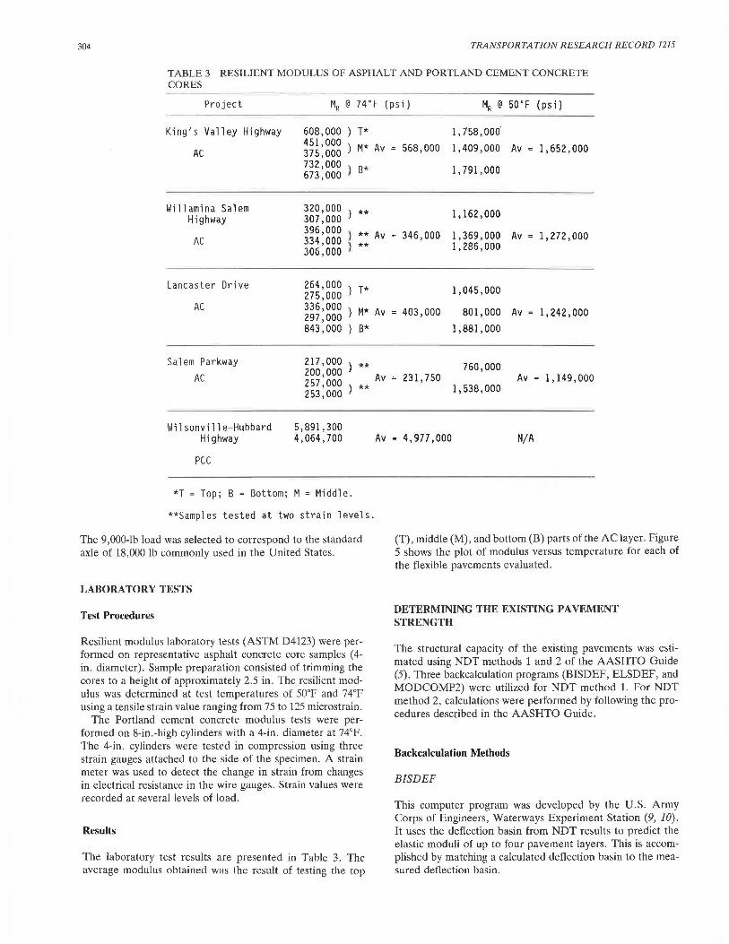
TABLE 3 RESILIENT MODULUS OF ASPHALT AND PORTLAND CEMENT CONCRETE CORES

Project MR @ 74 ° F (psi) MR@ 50'F (psi)

King's Va 11 ey Highway

AC

Willamina-Salem Highway

AC

Lancaster Drive

AC

Salem Parkway

AC

Wilsonville-Hubbard Highway

PCC

608,000 451,000 375,000 732,000 673,000

320,000 307,000 396,000 334,000 306,000

264,000 275,000 336,000 297,000 843,000

217,000 200,000 257,000 253,000

5,891,300 4,064,700

}

) }

*T = Top; B = Bottom; M = Middle.

T*

M*

13*

**

** **

T*

M*

B*

**

**

**Samples tested at two strain levels.

The 9,000-lb load was selected to correspond to the standard axle of 18,000 lb commonly used in the United States.

LABORATORY TESTS

Test Procedures

Resilient modulus laboratory tests (ASTM D4123) were performed on representative asphalt concrete core samples ( 4-in. diameter). Sample preparation consisted of trimming the cores to a height of approximately 2.5 in. The resilient modulus was determined at test temperatures of 50°F and 74°F using a tensile strain value ranging from 75 to 125 micros train.

The Portland cement concrete modulus tests were performed on 8-in.-high cylinders with a 4-in. diameter at 74°F. The 4-in. cylinders were tested in compression using three strain gauges attached to the side of the specimen. A strain meter was used to detect the change in strain from changes in electrical resistance in the wire gauges. Strain values were recorded at several levels of load.

Results

The laboratory test results are presented in Table 3. The average modulus obtained was the result of testing the top

1,758,000

Av 568,000 1,409,000 Av 1,652,000

1,791,000

1,162,000

Av 346,000 1,369,000 Av 1,272,000 1,286,000

1,045,000

Av 403,000 801,000 Av 1,242,000 1,881,000

760,000 Av 231,750 Av 1,149,000

1,538,000

Av 4,977,000 N/A

(T), middle (M), and bottom (B) parts of the AC layer. Figure 5 shows the plot of modulus versus temperature for each of the flexible pavements evaluated.

DETERMINING THE EXISTING PAVEMENT STRENGTH

The structural capacity of the existing pavements was estimated using NDT methods 1 and 2 of the AASHTO Guide (5). Three backcalculation programs (BISDEF, ELSDEF, and MODCOMP2) were utilized for NDT method 1. For NDT method 2, calculations were performed by following the procedures described in the AASHTO Guide.

Backcalculation Methods

BISDEF

This computer program was developed by the U.S. Army Corps of Engineers, Waterways Experiment Station (9, 10). It uses the deflection basin from NDT results to predict the elastic moduli of up to four pavement layers. This is accomplished by matching a calculated deflection basin to the measured deflection basin.

Zhou et al.

-~ -

102

45 50 55 60

-+-

King's Valley Willamina-Salem

-o- Lancaster Drive -+- Salem Parkway

65 70 75

305

80

Temperature • F

FIGURE 5 Plot of modulus vs. temperature.

To determine the layer moduli, the basic inputs include initial estimates of the elastic layer pavement characteristics as well as deflection basin values. Inputs for each layer include layer thickness, probable modulus range, initial estimate of modulus, and Poisson's ratio. For the deflection basin, the required inputs are load and load radius of an NDT device, deflections at a number of sensor locations , and a maximum acceptable error in deflection matching.

The modulus of any layer may be assigned or computed. If assigned, the value is based on the properties of the material at the time of deflection testing. The number of layers with unknown modulus values cannot exceed the number of measured deflections.

The program is solved using an iterative process that provides the best fit between measured deflection and computed deflection basins. This is done by determining the set of moduli that minimizes the error sum between the computed deflection and measured deflections. BISDEF uses the BISAR program as a subroutine for stress and deflection computations and is capable of handling multiple wheel loads and variable interface friction. BISDEF supports the 8087 or 80287 math coprocessor and runs on IBM-compatible microcomputers.

ELS DEF

This program is a modification of the program BISDEF (11). The modification was performed by Brent Rauhut Engineers and uses the computer program (ELSYM5) developed at the University of California at Berkeley (12). The input data and output results are basically the same as those of the BISDEF program.

ELSDEF has been compiled with the Microsoft FORTRAN Compiler to run on IBM-compatible microcomputers. Two versions are available: the standard version and an 8087 math coprocessor chip version.

MODCOMP2

This program was developed by Irwin (13) of Cornell University. The program utilizes the Chevron elastic layer computer program for determining the stresses, strains , and deflections in the pavement system. As in BISDEF and ELSDEF, there is no closed-form solution for determining layer moduli from surface deflection data. Thus, an iterative approach is used that requires an input of initial or estimat.::d moduli for each layer. The basic iterative process is repeated for each layer (beginning at the bottom) until the agreement between the calculated and measured deflections is within the specified tolerance or until the maximum number of iterations has been reached.

Backcalculation Results

Tables 4 to 8 show the backcalculation results using both the FWD and Dynaflect data on all five project sites. The backcalculation was carried out using the preceding three programs with three different procedures in an attempt to obtain consistent results. Procedure 1 used a fixed surface layer modulus for each project site to determine moduli of the base and subgrade . The surface layer modulus was based on the laboratory test results. Procedure 2 used both a fixed surface

TABLE4 BACKCALCULATED MODULI (psi) FOR KING'S VALLEY HIGHWAY

a) Procedure 1 - Fixed Surface Modulus

FWD D~naflect Location

Identification Layer* BISDEF ELSDEF MDDCOMP2 BISDEF ELS DEF MODCOMP2

3 Base 1,000 1, 100 N/S** 10,200 9,400 20' 700 Subgrade 60,000 60,000 36,600 32,900 27,600

4 Base 1,000 1,000 3,000 7,400 5,700 10,100 Subgrade 60,000 60,000 12,000 39,400 40,800 33,100

5 Base 1,000 1,000 N/S 5,300 3,800 6,300 Subgrade 60,000 60,000 39,500 53' 200 41,500

8 Base 1,000 1,000 N/S 14,200 13,600 28,500 Subgrade 60,000 60,000 32,300 27,500 25,500

18 Base 1,000 1,000 N/S 7,300 5,500 9,500 Subgrade 60,000 60,000 46,700 51,200 41,500

*Surfac ing layer modulus = 1. 200, 000 ps i, determined at 60 ' F from laboratory tests (Fig. 5). **N/S = no solution

Value 1,000 is low limit of modulus range for base while 60,000 is high limit for subgrade .

b) Procedure 2 - Fixed Surface and Subgrade Modulus


Identification Layer* BISDEF ELS DEF MODCOMP2 BISDEF ELS DEF MODCOMP2

3 Base 9.600 2,700 N/S*** 12,300 8,500 N/S Subgrade** 10,600 10, 600 35,000 35,000

4 Base 9,300 2,700 N/S 9,800 7,200 N/S Subgrade 10 ,700 10,700 35,000 35,000

5 Base 6, 100 2,300 N/S 8,500 6, 100 N/S Subgrade 11 ,700 11. 700 32,900 32,900

8 Base 6.100 2,300 N/S 15,600 9,900 N/S Subgrade 11, 600 11. 600 32,900 32,900

18 Base 5,000 2,300 N/S 10,000 7, 700 N/S Subgrade 13,400 13,400 39,900 39,900

*Surfacing layer modulus = 1,200,000 psi, determined at 60'F from laboratory tests (Fig . 5) . **Subgrade modulus was determined using the equation: Esg = PSf)/(rdr) .

***N/S = no solution.

c) Procedure 3 - Fixed Subgrade Modulus


Identification Layer* BIS DEF ELS DEF MODCOMP2 BISDEF ELSDEF MODCOMP2

3 Surf ace 472,000 842,300 668,800 1,032,500 1,125,300 3,500 , 500 Base 24,700 3,900 8,600 12,200 9,000 4,200 Subgrade 10,600 10,600 10 ,600 35,000 35,000 35,000

4 Surface 489,700 853 , 700 719 '400 913,800 973,500 3,228 ,500 Base 23' 100 3,800 7,600 10,300 8, 100 3,400 Subgrade 10,700 10,700 10,700 35,000 35,000 35,000

5 Surf ace 427,800 677 ,400 619,400 687,800 948' 100 2,829,900 Base 16,500 3,800 6,000 9,800 6,800 3,400 Subgrade 11, 700 11, 700 11. 700 32,900 32,900 32,900

8 Surface 426, 100 673,900 655,400 1,225,500 1. 465,000 3,717,300 Base 16,600 3,900 5,500 13,800 8,500 4,600 Subgrade 11,600 11, 600 11, 600 32,900 32,900 32,900

18 Surface 379,600 597' 100 554,800 756,500 1,062,300 3,250,300 Base 14,200 3,900 5,600 13,400 8,000 3,700 Subgrade 13', 400 13,400 13,400 39,900 39,900 39,900

*Subgrade modulus was determined using the equation : Esg = (PSf)/(rdr) .

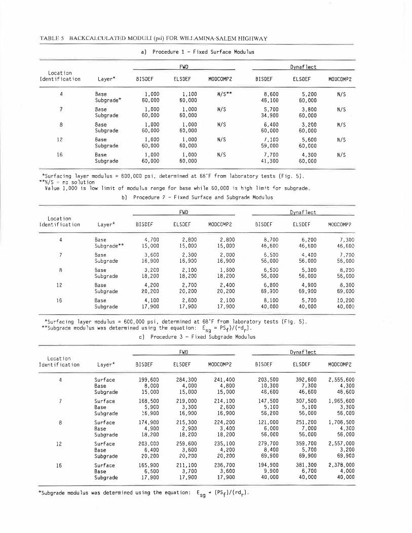
TABLE 5 BACKCALCULATED MODULI (psi) FOR WILLAMINA-SALEM HIGHWAY

a} Procedure 1 - Fixed Surface Modulus

FWD Dynaflect Location

Identificat ion Layer* BISDEF ELS DEF MODCOMP2 BISDEF ELSDEF MODCOMP2

4 Base 1,000 1,100 N/S** 8,600 5,200 N/S Subgrade* 60,000 60,000 46, 100 60,000

7 Base 1,000 1,000 N/S 5,700 3,800 N/S Subgrade 60,000 60,000 34,900 60,000

8 Base 1,000 1,000 N/S 6,400 3,200 N/S Subgrade 60,000 60,000 60,000 60,000

12 Base 1,000 1,000 N/S 7' 100 5,600 N/S Subgrade 60,000 60,000 59,000 60,000

16 Base 1,000 1,000 N/S 7,700 4,300 N/S Subgrade 60,000 60,000 41, 300 60,000

*Surf acing layer modulus= 600 ,000 psi, determined at 6B"F from labora t ory tests (F ig. 5). **N/S = no solution

Value 1,000 is low limit of modulus range for base while 60,000 i s high limit for subgrade .

b} Procedure 2 - Fi xed Surface and Subgrade Modulus

FWD Dynaf lect Location

Identification Layer* BIS DEF EL SDEF MODCOMP2 BI SDEF EL S DEF MODCOMP2

4 Base 4,700 2,800 2,800 8 , 700 6,200 7,300 Subgrade** 15,000 15,000 15,000 46 , 600 46,600 46,600

7 Base 3 , 600 2,300 2,000 6,500 4,400 7, 200 Subg rade 16 ,900 16,900 16,900 56, 000 56,000 56,000

8 Base 3,200 2' 100 1,600 6,500 5,300 8,200 Subg rade 18, 200 18,200 18,200 56,000 56,000 56,000

12 Base 4,200 2 ,700 2,400 6,800 4,900 8,300 Subgrade 20,200 20,200 20,200 69,900 69,900 69,000

16 Base 4' 100 2,600 2,100 8, 100 5 ,700 10,200 Subgrade 17,900 17,900 17,900 40,000 40,000 40,000

*Surfac ing layer modulus = 600 , 000 ps i , determined at 68" F f r om laboratory test s (Fig . 5) . **S ubgrade modulus was determined using the equation : Esg = PSf)/(rdr).

c) Procedure 3 - Fi xed Subg rade Modulus

FWD Dynaf lect Locat ion

Ident ification Layer* BISDEF ELSDEF MODCOMP2 BISDEF ELSDEF MODCOMP2

4 Surface 199,600 284,300 241, 400 203,500 392,600 2,555 , 600 Base 8,000 4,000 4,800 10' 300 7,300 4,300 Subgrade 15,000 15,000 15,000 46,600 46,600 46,600

7 Surface 168,500 219,000 214,100 147,500 307,500 1,965,600 Base 5,900 3,300 2,600 5,100 5, 100 3,300 Subgrade 16,900 16,900 16,900 56,200 56,000 56,000

8 Surface 174,900 215 , 300 224,200 121 , 000 251 , 200 1,706 ,500 Base 4,900 2,900 3,400 6,000 7,000 4,300 Subgrade 18,200 18,200 18,200 56,000 56,000 56,000

12 Surface 203,000 259,600 235.100 279,700 359' 700 2,557,000 Base 6,400 3,600 4, 200 8,400 5,700 3,200 Subgrade 20,200 20,200 20,200 69,900 69,900 69,900

16 Surface 165,900 211.100 236 , 700 194,900 381,300 2,378,000 Base 6,500 3 ,700 3, 600 9,900 6,700 4,000 Subgrade 17,900 17' 900 17,900 40,000 40,000 40,000

*Subgrade modulus was determined using the equation: Esg = (PSf)/(rdr) .

TABLE 6 BACKCALCULATED MODULI (psi) FOR LANCASTER DRIVE



Identification Layer* BISDEF ELSDEF MODCOMP2 BISDEF ELSDEF MOOCOMP2

2 Base 2,100 1,900 2,000 11, 700 17,900 17,800 Subgrade* 20,800 20,600 19,800 20,400 4,000 17,500

3 Base 1,700 1,400 1,300 9,300 11,700 13,400 Subgrade 60,000 51. 200 86,400 21.800 4,000 19' 100

14 Base 1,800 1,500 N/S** 9,300 11,700 13,300 Subgrade 33,700 30, 100 20' 100 4,400 17,500

17 Base 2' 100 1,800 1,800 14,400 25,600 22,600 Subgrade 31, 600 21,700 22,900 23,300 4, 100 19 ,700

19 Base 2,500 2,300 2,300 18,800 21.400 25' 100 Subgrade 17,400 10,800 13,300 16,500 12,800 14,700

*Surfacing layer modulus = 1,000,000 psi, determined at 57"F from laboratory tests (Fig. 5) . **N/S = no solution; Value 60,000 is high limit of modulus range for subgrade.



Identification Layer* BISDEF ELS DEF MODCOMP2 BISDEF ELS DEF MODCOMP2

2 Base 10,600 4,200 5, 100 14,500 10,400 N/S*** Subgrade** 8,700 8,700 8,700 18' 100 18,100

3 Base 7,400 3,400 4, 100 12 ,700 9,400 N/S Subgrade 9,300 9,300 9,300 18,100 18' 100

14 Base 8,600 3,400 4, 100 12,500 9,000 N/S Subgrade 8,500 8,500 8,500 17,000 17,000

17 Base 9,400 3,900 5,000 16,400 12,300 N/S Subgrade 8,800 8,800 8,800 21,500 21,500

19 Base 10,000 3,800 5,600 23' 100 14,500 N/S Subgrade 7,700 7,700 7,700 15' 100 15' 100

*Surfacing layer modulus= 1,000,000 psi, determined at 57"F from laboratory tests (Fig . 5) . **Subgrade modulus was determined using the equation: Esg = PSf)/(rdr).

***N/S = no solution



Identification Layer* BISDEF ELS DEF MDDCOMP2 BISDEF ELS DEF MODCOMP2

2 Surf ace 287,000 647' 100 585,300 383,400 987,300 N/S** Base 26,500 6,200 8,300 22,000 10,400 Subgrade* 8,700 8,700 8,700 18' 100 18' 100

3 Surf ace 312,000 635,900 537,200 249,300 1,139,600 N/S Base 19,300 4,900 7' 100 21,700 B,700 Subgrade 9,300 9,300 9,300 18' 100 18,100

14 Surface 405,300 765,100 865,000 477' 200 882,500 N/S Base 18,700 4,600 4,800 17,500 9,600 Subgrade 8,500 8,500 8,500 17,000 17,000

17 Surface 335,800 734,200 621,900 490,200 1,077. 000 N/S Base 23,200 5,100 7,700 22,200 11,600 Subgrade 8,800 8,800 8,800 21,500 21,500

19 Surface 390,800 834,800 567,500 692,600 1,398, 500 N/S Base 21,600 4,300 9,200 33,700 11,700 Subgrade 7,700 7,700 7,700 15' 100 15' 100

*Subgrade modulus was determined using the equation : Esg = (PSf)/(rdr) . **N/S = no solution

Zhou et al.

TABLE 7 BACKCALCULATED MODULI (psi) FOR SALEM PARKWAY

Location Identification

7

9

12

15

17

Layer*

CT Base/Subbase Subgrade*

CT Base/Subbase Subgrade





BISDEF

1. 020' 000 18,600

690' 900 23,400

805,200 24,600

727,700 19 .700

697,400 27,200

FWD

ELS DEF

501,200 15,300

681,800 16,500

508,700 12,300

409,600 14,500

491,800 13 ,700

MODCOMP2

365,300 19, 1 OD

255,400 31, 300

299,300 23,400

459,400 20,800

250,600 28,200

BISDEF

523,000 34,300

439,600 35' 100

543,900 35,000

400,800 31. 300

564,400 25,800

Dynaf lect

ELS DEF

1,497,300 14' 100

981,200 14,600

1,035,500 14,400

896,100 14,800

1,240,600 10' 100

MODCOMP2

183,000 35,600

154,100 36, 300

222,700 34,800

194,900 29,900

200,300 27,700

*Surfacing layer modulus = 500,000 psi, determined at 67"F from laboratory tests (Fig. 5) .

Location Identification

7

9

12

15

17


Layer*

CT Base/Subbase Subgrade*





BISDEF

751 , 300 21,600

577. 000 32 , 600

671. 500 25,400

581,800 23,800

600,400 29,600

FWD

ELSDEF MDDCDMP2

239,000 260,800 21,600 21,600

207,100 229,800 32,600 32,600

223,700 240,000 25,400 25,400

189,600 314,000 23,800 23,800

212,600 220,400 29,600 29,600

BISDEF

585,600 32,900

516,000 33,000

604, 700 33,000

463,800 29,500

663,300 24,400

Dynaflect

ELSDEF MODCOMP2

420,100 214,600 32,900 32,900

375,900 184,400 33,000 33,000

404,400 249,700 33,000 33,000

299,200 200,900 29,500 29,500

340,500 262,300 24,400 24,400

*Surfacing layer modulus= 500,000 psi, determined at 67"F from laboratory tests (Fig. 5) . **Subgrade modulus was determined using the equation : Esg = PSf)/(rdr).


FWD Dynaflect Location

Identification

7

9

12

15

17

Layer*

Surface CT Base/Subbase

Subgrade*


Subgrade


Subgrade

Surf ace CT Base/Subbase

Subgrade

Surf ace CT Base/Subbase

Subgrade

BIS DEF

5,813,400 273,400 21. 600

919,500 476,600 32,600

5,127,600 252,800 25,400

510,400 556, 100 23,800

4,408,300 230,100 29,600

ELSDEF

7,420,300 100,000 21,600

3,387,000 100,000 32,600

4,224,000 100,000 25,400

3,111.700 100,000 23,800

3 ,722. 200 100,000 29,600

MODCDMP2

8,224,900 130,200 21,600

1.762. 400 190,900 32,600

4,807,000 153,900 25,400

526,900 311,100

23,800

3,234,500 162,300 29,600

*Subgrade modulus was determined using the equation: Es = PSf)/(rdr). Value 100,000 is the low limit of modulus range for the er base/subbase .

BISDEF

3,459,500 405,600 32,900

2,549,700 370. 800 33,000

590, 117 925,800 33,000

1,030,600 609,900 29,500

1,673,100 608,400 24,400

ELS DEF

9,201,800 100,000 32,900

8,157,200 100,000 33,000

9,467,400 100,000 33,000

9,246,700 109,000 29,500

9,186,500 100,000 24,400

MODCOMP2

6,264,500 125,000 32. 900

6,360,600 102,100 33,000

6,378,500 147,800 33,000

6,673,100 109,100 29,500

4, 106' 600 174,000 24,400

309

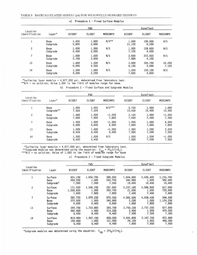
TABLE 8 BACKCALCULATED MODULI (psi) FOR WILSONVILLE-HUBBARD HIGHWAY


FWD D:inaf lect Location

Identification Layer* BISDEF ELSDEF MDDCDMP2 BISDEF ELSDEF MODCOMP2

Base 1,000 1,000 N/S** 1,000 106,900 N/S Subgrade 5,900 3,900 ll, 100 6,200

2 Base 1,000 1,000 N/S 1,000 128 ,600 N/S Subgrade 6,400 3,900 7. 700 4,000

7 Base 1,000 1,000 N/S 2,600 215,000 N/S Subgrade 5,700 3,800 7,900 4, 100

13 Base 1,000 1,000 N/S 1,000 185.700 24,200 Subgrade 6,900 4,500 8, 100 3,900 7, 100

14 Base 1,000 1, 000 N/S 1,000 130,100 N/S Subgrade 5,000 3,200 7,600 4,800

*Surfacing layer modulus= 4,977,000 psi, determined from laboratory test . **N/S = no solution; Value 1,000 is low limit of modulus range for base.


FWD D:inaflect Location

Identification Layer* BISDEF ELS DEF MODCOMP2 BIS DEF ELSDEF MODCOMP2

Base 1,000 1,000 N/S*** 2 ,700 1,000 1,600 Subgrade** 7,300 7,300 10,400 10,400 10 ,400

2 Base 1,000 1,000 <1,000 2, 100 1,000 <1 , 000 Subgrade 7,800 7,800 7,800 7,400 7,400 7, 400

7 Base 1,000 1,000 <1, 000 1,000 1,000 4,900 Subgrade 6,600 6,600 6,600 7,800 7,800 7,800

13 Base 1,000 1,000 <l,000 1,000 1,000 2. 200 Subgrade 8,400 8,400 8,400 7,500 7,500 7,500

14 Base 1,000 1,000 N/S 1,000 1,000 <l,000 Subgrade 6,400 6,400 7,600 7,600 7,600

*Surfacing layer modulus= 4,977 ,000 psi, determined from laboratory test . **Subgrade modulus was determined using the equation : E = PSf)/(rdr).

***N/S = no solution; Value of 1,000 is low limit of modu~Hs range for base


FWD D:inaflect Location

Identification Layer BISDEF ELS DEF MODCOMP2 BISDEF ELSDEF MODCDMP2

Surf ace 424, 100 1,634,700 389,000 1,944,000 4,436,400 1,255,700 Base 354,200 1,000 343,700 242,900 1,000 502,000 Subgrade* 7,300 7,300 7,300 10,400 10,400 10,400

2 Surface 171. 500 1. 548' 700 297,600 3,237,100 3,598 ,900 817,900 Base 1.028 ,600 1,000 390.700 21. 000 1,000 735,600 Subgrade 7,800 7,800 7,800 7,400 7,400 7,400

7 Surf ace 595, 700 1,979,200 676,300 4,982,600 4,056,400 906,500 Base 272,600 1,000 340,900 2,200 l,000 1,124,200 Subgrade 6,600 6,600 6,600 7,800 7,800 7,800

13 Surface 345, 700 1.733,800 393. 700 3,750,100 3 ,757 ,200 877 ,900 Base 582,000 1, 000 314,200 3,400 1,000 479,500 Subgrade 8,400 8,400 8,400 7,500 7,500 7,500

14 Surf ace 810,900 1. 547 ,700 858,200 2 ,631,800 3, 167 ,700 872,900 Base 159,000 1,000 131. 600 24, 100 l , 000 466,000 Subgrade 6,400 6,400 6,400 7,600 7,600 7,600

*Subgrade modulus was determined using the equation: Esg = (PSf)/(rdr) .

Zhou et al.

layer modulus and a preestimated subgrade modulus to solve for the modulus of the base layer. The subgrade modulus was determined using the following AASHTO equation (5):

Esg = (PS1 )l(d,r)

where

Esc = in situ subgrade modulus of elasticity (psi); P = dynamic load of NDT device; d, = measured NDT deflection (mils) at a radial distance

(r) from the plate load center; r = radial distance (in.) from the plate load center; and

S1 = subgrade modulus prediction factor, which is a function of radius of NDT load plate, Poisson's ratio, and effective thickness of the pavement.

Procedure 3 used the preestimated subgrade modulus alone to solve for the surface and base layer moduli. Procedure 4 used no fixed value. With this procedure, all layers were considered as unknowns for the program to determine moduli. Since three variables were involved, the computing time was significantly increased and the calculated moduli were also subject to variation with the seed moduli. Because of inconsistent results obtained using this procedure, no further discussion is presented.

Procedure 1

Using this procedure, the surfacing modulus for each project was determined from laboratory tests and used as a fixed value in the backcalculation. For Salem Parkway, base and sub base were treated as one layer, thus eliminating one variable for determining modulus. The results from three programs using FWD data indicate that the King's Valley Highway, Willamina-Salem Highway, and Lancaster Drive sites have a weak base layer. On the other hand, using Dynaflect data, a consistently higher modulus for the base layer was found. Results from BISDEF and ELSDEF are relatively close using both FWD and Dynaflect data . MODCOMP2 provided no solution in several cases . Results from three programs using the same NDT device are generally close.

Salem Parkway has a cement-treated base/subbase. Results from three programs reflect this fact. However, the backcalculated modulus values vary for each program. With FWD data, results from BISDEF are higher than those of both ELSDEF and MODCOMP2. With Dynaflect data, ELSDEF presents the highest modulus values among three programs. In all cases, MODCOMP2 provides the lowest values. Subgrade modulus values calculated from BISDEF and MODCOMP2 are relatively close for each NDT testing device, while ELSDEF gives a consistent lower modulus value using both FWD and Dynaflect data.

Wilsonville-Hubbard Highway is a PCC pavement. Its surfacing layer modulus is about 5 million psi as tested in the laboratory. When fixing this value and backcalculating the other two layer moduli, the program BISDEF predicts a very weak base using both FWD and Dynaflect data; ELSDEF gives different solutions using different NDT device data ; and MODCOMP2 fails to provide answers in most cases.

311

Procedure 2

This procedure used two known moduli to determine the third unknown modulus. The surfacing modulus was determined from the laboratory test, while the subgrade modulus was estimated using the AASHTO equation. Since only one variable (base) is defined, the difference, that of backcalculated moduli using different programs, can easily be seen. For all four flexible pavements, the program BISDEF presents a consistently higher modulus than ELSDEF and MODCOMP2. The results of this method show many similarities with those of procedure 1. A weak base at the King's Valley Highway, Willamina-Salem Highway, and Lancaster Drive project sites is indicated. A similar trend at Salem Parkway is also noted. For the PCC pavement at Wilsonville-Hubbard Highway, a very weak base layer i identified by all thr • programs using both FWD and Dynaflect data. Again, MOD OMP2 failed to give a solution in some test locations.

Procedure 3

The third procedure used an estimated subgrade modulus as a fixed input to solve for surface and base moduli. The results are presented in Tables 4c to 8c. Although the backcalculated moduli vary for each program, the results from each individual program are fairly clo e for the projects at King's Valley Highway, Willamina-Salem Highway , and Lancaster Drive. As would be expected, Willamina-Salem Highway would have the lowest modulus values since it had the highest measured deflection at NDT device load center, and King's Valley Highway would have high modulus because of its smaller deflection readings, while Lancaster Drive would stand in among these three project sites . The backcalculated results reflect this phenomenon very well. For Willamina-Salem Highway using BI -DEF results , the average modulus for the urface is about 180 ksi. The ave rage urface modulus for King . Valley Highway is close to 440 ksi and, for Lanca Ler Drive, approximate ly 350 ksi. The backcalculatet.I moduli for the ba e layer al seem reasonable. Values are generally uniform, with BISDEF giving a little higher modulus. For the cement-treated base/ ubba e project at Salem Parkway, the three programs give

inconsi tent results, as can be seen in Table 7c. Thi fact is also reflected in the Wilsonville-Hubbard Highway , which is a PCC pavement. It is therefore difficult to make a general prediction of pavement strength on these two projects based on the backcalculated moduli using procedure 3.

Existing Pavement Structural Capacity

The structural capacity of the existing pavements was determined using the backcalculation results. For NDT method 1, the SNxerr values for each test location were computed for both the FWD and Dynaflect using the backcalculated results from the BISDEF program. For King' · Valley Highway, Willamina-Salem Highway, and Lancaste r Drive , backcalculated moduli from procedure 3 were used to determine the N~crr

·ince they seemed m re rea onable compared with the other two procedures. For Salem-Parkway and Wilsonville-Hubbard Highway, procedure 1 results were used because of


TABLE 9 CALCULATED SN,ctr USING BISDEF RESULTS

FWD Di1naflect

NOT #1 NOT #2 NOT #1 NOT #2 Project Site Layer MR (ks i )* scxeff MR scxeff MR scxeff MR scxeff

King's Valley Highway Surf ace 439.0 3.84 3.70 923 . 2 3.17 8.15 Base 19 . 0 11.9 Subgrade 11.6 11. 6 35.1 35. l

Willamina-Salem Surf ace 182.4 1. 67 2.92 189 .3 1. 75 7.26 Highway Base 6.3 7.9

Subgrade 17.6 17.6 53 . 7 53.7

Lancaster Drive Surface 346.2 3.96 3.99 458 .5 4.33 8.12 Base 21.9 23 .4 Subgrade 8.6 8.6 18 . 0 18.0

Salem Parkway Surf ace 500 . 0 5.34 6.95 500 . 0 3.80 12.46 Base 788 . 2 494 .3 Subgrade 22 .7 26.3 32 .3 30.2

Wilsonville-Hubbard Surface 4977. 0 6.00 6.00** 4977. 0 6.00 6.00 Highway Base 1. 0 1.3

Subgrade 6.0 7.3 8.5 8. 1

*Average values **NOT method 2 is not applicable for the evaluation of rigid pavement systems. With this method, structural capacity is expressed in terms of the PCC layer and not the other layers.

inconsistent results of procedure 3 and a good agreement between procedures 1 and 2. The layer coefficients for the surface and base were determined based on the modulus values from the backcalculation.

For NDT method 2, the SNxeff values were determined using the procedures described previously, while the subgrade modulus was estimated using the AASHTO equation. The results for both methods are presented in Table 9.

The results generally indicate the following:

1. A fair agreement in calculating SNxeff between NDT methods 1 and 2 was found using FWD data.

2. While using Dynaflect data, the NDT method 2 results in much higher SNxerr values than NDT method 1 and also higher than those obtained using FWD data.

3. A maximum surface layer coefficient of 0.44 was used for asphalt concrete pavements. This may not reflect the true structural capacity of those surface layers with high modulus.

OVERLAY DESIGN

AASHTO Method

With the AASHTO method, overlay design was performed based upon the existing pavement structural capacity (SNxerr) and future traffic applications (W18). For each project, SNxeff values determined previously were used to estimate the remaining life of the existing pavement and, consequently, the thickness design. In determining the future overlay structural capacity (Sey), a 90 percent reliability level (R) was chosen for the Willamina-Salem Highway and Salem Parkway

projects. An 80 percent reliability was selected for King's Valley Highway, Lancaster Drive, and Wilsonville-Hubbard Highway. The overall standard deviation (S 0 ) was selected to be 0.35 for all five projects. The design serviceability loss (DSL) was set at 2.0 (4.2-2.2). The selection of the preceding values was primarily based on the functional class and location of the facility and the projected level of usage.

Knowing the future traffic (W18), reliability level (R), overall standard deviation (S0 ), design serviceability loss (DSL), and subgrade modulus (MR), the structural number (SNy) was determined.

The remaining life of the existing pavement (RLX) was estimated using the NDT approach. The advantage of this method is that historical traffic data are not required. Using this approach, the existing pavement condition is related to its initial structural capacity by a condition factor, ex. R LX is a function of the value for ex. The remaining life of overlaid pavements (RLY) was calculated based upon the projected future traffic applications and the ultimate number of repetitions to failure. The failure serviceability level (P1) was set at 2.0 for all five projects. After determining both RLX and RLY, the remaining life factor, FRL• was estimated.

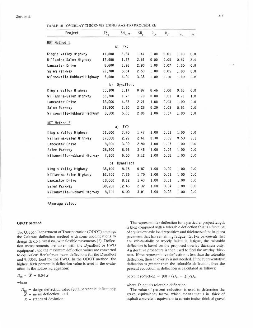
The required flexible overlay structural number, SN0 L, is a function of the structural capacity of the existing pavement (SNxerr), the overlaid pavement (SNY), and the remaining life factor (FRL). If this value is less than or equal to zero, no overlay is required. The thickness of an overlay is determined by dividing the SN oL by the layer coefficient of the surfacing material. For the five projects, the thickness of a flexible overlay was determined assuming a layer coefficient of 0.44 for the asphalt concrete. Summaries for both NDT method 1 and NDT method 2 are presented in Table 10.

Zhou et al. 313

TABLE 10 OVERLAY THICKNESS USING AASHTO PROCEDURE

Project E~g SNxeff SNY RLX RL Y FRL TAC

NDT Method 1 a) FWD

King's Valley Highway 11 , 600 3.84 l. 47 l.00 0.01 l.00 0.0 Willamina-Salem Highway 17,600 l.67 2.61 0.00 0.05 0.67 3.4 Lancaster Drive 8,600 3.96 2.90 l.00 0.07 l.00 0.0 Salem Parkway 22,700 5.34 2.58 l.00 0.05 l.00 0.0 Wilsonville-Hubbard Highway 6,000 6.00 3.35 l.00 0. IO l. 00 o.n

b) Dynaflect

King's Valley Highway 35' 100 3 .17 0.87 0.46 0.00 0.63 0.0 Willamina-Salem Highway 53,700 l. 75 l. 70 0.00 0.01 0. 71 l. 0

Lancaster Drive 18,000 4.33 2.21 l. 00 0.03 l.00 0.0 Salem Parkway 32,300 3.80 2.26 0.29 0.03 0.53 0.0

Wilsonville-Hubbard Highway 8,500 6.00 2.96 l. 00 0.07 l. 00 0.0

NDT Method 2 a) FWD

King's Valley Highway 11 ,600 3.70 l. 47 l.00 0.01 l.00 0.0

Willamina-Salem Highway 17 ,600 2.92 2.61 0.30 0.05 0.58 2.1

Lancaster Drive 8,600 3.99 2.90 1.00 0.07 1. 00 0.0

Salem Parkway 26,300 6.95 2.45 1.00 0.04 1.00 0.0

Wilsonville-Hubbard Highway 7,300 6. 00 3 .12 1. 00 0. 08 1.00 0.0

b) Dyna fl ect

King's Valley Highway 35 , 100

Wi 11 ami na-Sa l em Highway 53,700

Lancaster Drive 18,000

Salem Parkway 30,200

Wilsonville-Hubbard Highway 8, 100

*Average Values

ODOT Method

The Oregon Department of Transportation (ODOT) employs the Caltrans deflection method with some modifications to design flexible overlays over flexible pavements (1). Deflection measurements are taken with the Dynaflect or FWD equipment, and the maximum deflection values are converted to equivalent Benkelman beam deflections for the Dynaflect and 9,000-lb load for the FWD. In the ODOT method, the highest 80th percentile deflection value is used in the evaluation in the following equation:

D80 = X + 0.84 S

where

D80

= design deflection value (80th percentile deflection); X = mean deflection; and S = standard deviation.

8.15 0.87 1.00 0. 00 1.00 0.0

7.26 1. 70 l.00 0.01 1. 00 0.0

8 .12 1. 43 1.00 0. 01 1.00 0.0

12.46 2.32 1.00 0. 04 l.00 0.0

6.00 3.01 1.00 0.08 1. 00 0.0

The representative deflection for a particular project length is then compared with a tolerable deflection that is a function of equivalent axle load repetition and thickness of the in-place pavement that has remaining fatigue life. For pavements that are substantially or wholly failed in fatigue, the tolerable deflection is based on the proposed overlay thickness only. An iterative procedure is then used to find the overlay thickness. If the representative deflection is less than the tolerable deflection , then an overlay is not needed . If the representative deflection is greater than the tolerable deflection, then the perc:ent reduction in deflection is calculated as follows:

percent reduction = 100 • (D 80 - D,)ID80

where D, equals tolerable deflection . The value of percent reduction is used to determine the

gravel equivalency factor, which means that 1 in . thick of asphalt concrete is equivalent to certain inches thick of gravel

314

(4). The equivalent factor ranges from 1.52 to 2.5. A factor of 2.0 is used for this study.

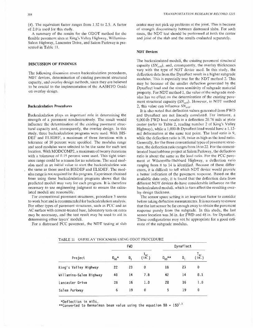
A summary of the results for the ODOT method for the flexible pavement sites at King's Valley Highway, WillaminaSalem Highway, Lancaster Drive, and Salem Parkway is presented in Table 11.

DISCUSSION OF FINDINGS

The following discussion covers backcalculation procedures, NDT devices, determination of existing pavement structural capacity, and overlay design methods, since they are believed to be crucial to the implementation of the AASHTO Guide on overlay design.

Backcalculation Procedures

Backcalculation plays an important role in determining the strength of a pavement nondestructively. The result would influence the determination of the existing pavement structural capacity and, consequently, the overlay design. In this study, three backcalculation programs were used. With BISDEF and ELSDEF, a maximum of three iterations with a tolerance of 10 percent were specified. The modulus range and seed modulus were selected to be the same for each test location. With MODCOMP2, a maximum of twenty iterations with a tolerance of 0.15 percent were used. This tight tolerance range could be a reason for no solutions. The seed modulus used as an initial value to start the backcalculation was the same as those used in BISDEF and ELSDEF. The modulus range is not required for this program. Experience obtained from using these backcalculation programs shows that the predicted moduli may vary for each program. It is therefore necessary to use engineering judgment to ensure the calculated moduli are reasonable.

For conventional pavement structures, procedure 3 seems to work best and is recommended for backcalculation analysis. For other types of pavement structures, such as PCC and an AC surface with cement-treated base, laboratory tests on cores may be necessary, and the test result may be used to aid in determining other layers' moduli.

For a distressed PCC pavement, the NDT testing at slab

TRANSPORTATION RESEARCH RECORD 1215

center may not pick up problems at the joint. This is because of strength discontinuity between distressed slabs. For such cases, the NDT test should be performed at both the center and joint of the slab and the results evaluated separately.

NDT Devices

The backcalculated moduli, the existing pavement structural capacity (SNxeff), and, consequently, the overlay thicknesses vary with the type of NDT device used. In this study, the defledion data from the Dynaflect result in a higher subgrade modulus. This is especially true for the NDT method 2. This may be because of the smaller deflection generated by the Dynaflect load and the stress sensitivity of subgrade material property. For NDT method 1, the value of the subgrade modulus has no effect on the determination of the existing pavement structural capacity (SNxeff). However, in NDT method 2, this value can influence SNxerr·

It is also noted that deflection values generated from FWD and Dynaflect are not linearly correlated. For instance, a 9,000-lb FWD load results in a deflection 20.76 mils at plate center (refer to Table 2, reading number 2 of King's Valley Highway), while a 1,000-lb Dynaflect load would have a 1.12-mil deformation at the same test point. The load ratio is 9, while the deflection ratio is 18, twice as high as the load ratio. Generally, for the three conventional types of pavement structure, the deflection ratio ranges from 16 to 22. For the cementtreated base/sub base project at Salem Parkway, the deflection ratio is about the same as the load ratio. For the PCC pavement at Wilsonville-Hubbard Highway, a deflection ratio ranging from 8 to 14 is identified. Because of these differences, it is difficult to tell which NDT device would provide a better indication of the pavement response. Based on the available data only, it is found that the deflection data from different NDT devices do have considerable influence on the backcalculated moduli, which in turn affect the resulting overlay design thickness.

The sensor space setting is an important factor to consider before taking deflection measurements. It is necessary to ensure that the last sensor be far enough away to obtain the pavement response purely from the subgrade. In this study, the last sensor location was 36 in. for FWD and 48 in. for Dynaflect. These configurations may not be appropriate for a good estimate of the subgrade modulus.

TABLE 11 OVERLAY THICKNESS USING ODOT PROCEDURE

FWD Dynaflect

Project Dao* Dt TAC

(in.} D ** 80 Dt TAC

(in.}

King's Valley Highway 22 23 0 18 23 0

Wi 11 ami na-Sa l em Highway 40 14 7.8 42 14 8.1

Lancaster Drive 28 16 1.0 28 16 1.0

Salem Parkway 6 19 0 5 19 0

~uer1eci1on in mils. l 5Dl. 3 **Converted to Benkelman beam value using the equation BB

Zhou et al.

Determination of SNx.cr

The existing structural capacity (SNxerr) of a pavement can be determined using either NDT method 1 or NDT method 2, although the background of these two methods differs. For NDT method 1, the determination of SNx.rr relies on deflection basin data, methods of estimating the modulus of each pavement layer, and the relationship between layer modulus and layer coefficient. For NDT method 2, SNxerr is determined from the maximum deflection as well as the in situ subgrade modulus . Ideally, these two methods should provide similar solutions. The results in this study (Table 9) show that the calculated SNx.rc using FWD data seems to give good correlation, while the SNx.rr values are less related when Dynaflect data are used. It should be noted that for NDT method 1, the layer coefficient for AC is restricted to a maximum value of 0.44; any modulus higher than 500 ksi would not contribute to the SNxerr value. For NDT method 2, there is no such restriction; the SNxerr is determined from the matching of the maximum deflection.

Overlay Design Methods

The overlay thicknesses determined from the two design methods, AASHTO and ODOT, are summarized in Table 12. As can be seen from the table, the King's Valley Highway and Salem Parkway projects have no need of an overlay. However, both procedures indicate that the Willamina-Salem Highway requires an overlay. The thickness of the required overlay varies for each method: the AASHTO NOT methods 1 and 2 require an overlay thickness ranging from 1 to 3.4 in . , while an overlay thickness of about 8 in . is required by the ODOT method. For the Lancaster Drive site, no overlay is required using both NOT methods 1 and 2, while results from the ODOT method show that an overlay of 1 in. is required. Since Lancaster Drive had been overlaid the previous year (1986), it would seem that the AASHTO procedure provided a more reasonable estimate. The Wilsonville-

315

Hubbard Highway is a PCC pavement. The structural capacity of this pavement is good, and no overlay is needed, as calculated using the AASHTO method. The pavement condition is bad, however, and cracking of slabs was found during the condition survey. It is possible that the determination of the SNxerr was not right. The existence of the slab cracking seems difficult to identify using the AASHTO method.

Preliminary analysis of these results seems to lead to either one of the following conclusions: the ODOT method provides an overdesign of the overlay thickness and the AASHTO method(s) provide a more reasonable result; or the ODOT method provides a reasonable design and the AASHTO method(s) provide an underdesign. Further large-scale investigation _on typical asphalt concrete and PCC pavements is needed to verify the conclusions reached thus far.

CONCLUSIONS AND RECOMMENDATIONS

Conclusions

Preliminary conclusions made from the data analyzed include:

1. The AASHTO method is based on the concept of reliability of design as well as the remaining life of the pavement; the ODOT method is based on the highest 80th percentile deflection value while the remaining life of the pavement is ignored.

2. A reliable backcalculation program is critical to implement NDT method 1. The study in this paper shows that the three backcalculation programs seem to work relatively well for the conventional pavement sections analyzed.

3. Good correlation was found between NDT methods 1 and 2 in determining the structural capacity using the FWD data. However, significant differences were also noted while using Dynaflect data .

4. The deflection data collected using FWD or Oynaflect can result in different overlay design. This conclusion is applied to both AASHTO and ODOT methods.

TABLE 12 COMPARISON OF TWO OVERLAY DESIGN METHODS

AASHTO

Project Site

King ' s Valley Highway*

Willam i na-Sa l em Highway

Lanca ster Drive

Salem Parkway

Wil sonville-Hubba rd Highway**

NOT Method 1 NOT Method 2 ODOT

FWD Dynaflect FWD Dynaflect FWD Dynaflect

0 0

3.4 1.0

0 0

0 0

0 0

0

2. 1

0

0

0

0

0

0

0

0

0

7.8

1.0

0

N/A

0

8 . 1

1.0

0

*This pavement would probably require a chip seal t o prevent water infiltrati on. It s st ructural capacity is good .

**This is a PCC pavement . The structu ral capacity of this pavement is good ; the thickness of t he over lay would be controlled by reflec t ion cracking . N/ A = not appl icab l e.

316

Recommendations for Implementation

The following recommendations are based upon the results of this study:

1. Although the backcalculation program may produce a set of moduli for a pavement structure, laboratory tests may still be necessary for providing an estimate and/or verification of the backcalculated values. In some cases, the laboratory results should be used in the program as a fixed input to determine the moduli of the other layers. For conventional pavements, subgrade modulus may be estimated using the AASHTO equation and used as a fixed input to solve for other layers' moduli.

2. Engineering judgment must be made in selecting the layer coefficients. This is particularly difficult when extremely high and low moduli are involved.

3. A comparison of the two design procedures (AASHTO and ODOT) reveals significant differences between the calculated overlay designs. The reason for these differences needs to be understood before the 1986 AASHTO procedure can be applied to routine design work.

ACKNOWLEDGMENTS

The work presented in this report was conducted as a part of a Highway Planning and Research (HP&R) project funded by the U.S. Department of Transportation, Federal Highway Administration (FHW A), and Oregon Department of Transportation (ODOT). The authors are grateful for the support of the Surfacing Design Unit (ODOT) for collecting the data contained in the report. They are also grateful to the Department of Civil Engineering, Oregon State University (OSU), for providing the laboratory and computer facilities required to complete the needed work. Laurie Dockendorf and Peggy Offutt of OSU's Engineering Experiment Station typed the paper.

REFERENCES

1. Flexible Pavement Design Procedure. Oregon State Highway Division, Salem, 1956.

TRANSPORTATION RESEARCH RECORD 1215

2. Thickness Design for Concrete Highway and Street Pavements. Portland Cement Association, Skokie, Ill., 1984.

3. AASHTO Interim Guide for Design of Pavement Structures. American Association of State Highway and Transportation Officials, Washington, D.C., 1981.

4. Asphalt Concrete Overlay Design Manual. California Department of Transportation, Sacramento, 1979.

5. AASHTO Guide for Design of Pavement Structures. American Association of State Highway and Transportation Officials, Wnshington, D .C., 1986.

6. H. Zhou , R. G. Hicks, and R. Noble. Development of an Improved Overlay Design Procedure for Oregon: Vol. Ill-Field Manual. FHWA-OR-RD-88-03C. FHWA, U.S. Department of Transportation, November 1987.

7. 0. Tholen. Falling Weight Deflectometer, A Device for Bearing Capacity Measurements: Properties and Performance. Department of Highway Engineering, Royal Institute of Technology, Stockholm, Sweden, 1980.

8. 0. Tholen, J. Sharma, and R . Terrel. Comparison of Falling Weight Deflectometer with Other Deflection Testing Devices. In Transportation Research Record 1007, TRB, National Research Council, Washington, D.C., 1985, pp. 20-26.

9. A. J. Bush and D . R. Alexander. Pavement Evaluation Using Deflection Basin Measurement and Layered Theory. In Transportation Research Record 1022, TRB, National Research Council, Washington, D.C., 1985, pp. 16-25.

10. A. J. Bush III. Nondestructive Testing for Light Aircraft Pavements: Phase II-Development of Nondestructive Evaluation Methodology. Final Report FAA-RD-80-9-II. FAA, U.S. Department of Transportation, November 1980.

11. R. L. Lytton, F. L. Roberts, and S. Stoffels . Determination of Asphaltic Concrete Pavement Structural Properties by Nondestructive Testing. Final Report, NCHRP, Project 10-27. TRB, National Research Council, Washington, D .C., 1986.

12. R. G. Hicks and R. L. McHattie. Use of Layered Theory in the Design and Evaluation of Pavement Systems. Report FHWA-AKRD-83-8. FHWA, U.S. Department of Transportation, July 1982.

13 . L. H. Irwin. User's Guide to MODCOMP2, Version 2.1. Local Roads Program, Cornell University, Ithaca, N.Y., November 1983.

The opinions expressed in this paper are those of the authors and not necessarily those of FHWA or Oregon DOT.

Publication of this paper sponsored by Committee on Pavement Rehabilitation.

evaluation of the 1986 aashto overlay design...

Documents