RESEARCH Open Access

Evaluation of statistical methods used inthe analysis of interrupted time seriesstudies: a simulation studySimon L. Turner1, Andrew B. Forbes1, Amalia Karahalios1, Monica Taljaard2,3 and Joanne E. McKenzie1*

Abstract

Background: Interrupted time series (ITS) studies are frequently used to evaluate the effects of population-levelinterventions or exposures. However, examination of the performance of statistical methods for this design hasreceived relatively little attention.

Methods: We simulated continuous data to compare the performance of a set of statistical methods under a rangeof scenarios which included different level and slope changes, varying lengths of series and magnitudes of lag-1autocorrelation. We also examined the performance of the Durbin-Watson (DW) test for detecting autocorrelation.

Results: All methods yielded unbiased estimates of the level and slope changes over all scenarios. The magnitudeof autocorrelation was underestimated by all methods, however, restricted maximum likelihood (REML) yielded theleast biased estimates. Underestimation of autocorrelation led to standard errors that were too small and coverageless than the nominal 95%. All methods performed better with longer time series, except for ordinary least squares(OLS) in the presence of autocorrelation and Newey-West for high values of autocorrelation. The DW test for thepresence of autocorrelation performed poorly except for long series and large autocorrelation.

Conclusions: From the methods evaluated, OLS was the preferred method in series with fewer than 12 points,while in longer series, REML was preferred. The DW test should not be relied upon to detect autocorrelation, exceptwhen the series is long. Care is needed when interpreting results from all methods, given confidence intervals willgenerally be too narrow. Further research is required to develop better performing methods for ITS, especially forshort series.

Keywords: Autocorrelation, Interrupted time series, Public health, Segmented regression, Statistical methods,Statistical simulation

BackgroundInterrupted time series (ITS) studies are frequently usedto evaluate the impact of interventions or exposures thatoccur at a particular point in time [1–4]. Although ran-domised trials are the gold standard study design, ran-domisation may be infeasible in the case of policy

evaluation or interventions that are implemented at apopulation level. Randomization also is not an optionfor retrospective evaluation of interventions or exposuressuch as natural disasters or pandemics. The use of anITS design may be considered in these situations, as theyare one of the strongest non-randomised experimentaldesigns [2, 5–9].In an ITS study, observations are collected at regular

time points before and after an interruption, and oftenanalysed in aggregate using a summary statistic (e.g.

© The Author(s). 2021 Open Access This article is licensed under a Creative Commons Attribution 4.0 International License,which permits use, sharing, adaptation, distribution and reproduction in any medium or format, as long as you giveappropriate credit to the original author(s) and the source, provide a link to the Creative Commons licence, and indicate ifchanges were made. The images or other third party material in this article are included in the article's Creative Commonslicence, unless indicated otherwise in a credit line to the material. If material is not included in the article's Creative Commonslicence and your intended use is not permitted by statutory regulation or exceeds the permitted use, you will need to obtainpermission directly from the copyright holder. To view a copy of this licence, visit http://creativecommons.org/licenses/by/4.0/.The Creative Commons Public Domain Dedication waiver (http://creativecommons.org/publicdomain/zero/1.0/) applies to thedata made available in this article, unless otherwise stated in a credit line to the data.

* Correspondence: joanne.mckenzie@monash.edu1School of Public Health and Preventive Medicine, Monash University, 533 StKilda Road, Melbourne, Victoria, AustraliaFull list of author information is available at the end of the article

Turner et al. BMC Medical Research Methodology (2021) 21:181 https://doi.org/10.1186/s12874-021-01364-0

mean, proportion) within a time interval (e.g. weekly,monthly, or annually). A key feature of the design is thatdata from the pre-interruption interval can be used toestimate the underlying secular trend. When this trendis modelled correctly, it can be projected into the post-interruption interval, providing a counterfactual for whatwould have occurred in the absence of the interruption.From this counterfactual, a range of effect measures canbe constructed that characterise the impact of the inter-ruption. Two commonly used measures include the‘change in level’ – which represents the sustained changeimmediately after the interruption, and the ‘change inslope’ – which represents the difference in trends beforeand after the interruption.A key feature of time series data is that there is the po-

tential for non-independence of consecutive data points(serial autocorrelation) [10]. In the presence of positiveautocorrelation, statistical methods that do not accountfor this correlation will give spuriously small standarderrors (SEs) [11]. Several statistical methods are availableto account for autocorrelation, such as Prais-Winstengeneralised least squares or the Newey-West correctionto SEs, or to directly model the error, such as autore-gressive integrated moving averages (ARIMA). Further,several methods are available for testing for the presenceof autocorrelation, with the Durbin-Watson test for lag-1 autocorrelation being the most commonly used [4, 6].While the performance of some of these methods hasbeen examined for time series data [12, 13], their per-formance in the context of ITS studies has received rela-tively less attention [11, 14, 15].In this study, we therefore aimed to examine the per-

formance of a range of statistical methods for analysingITS studies with a continuous outcome using segmentedlinear models. We restrict our evaluation to ITS designswhere there is a single interruption, with an equal num-ber of time points pre and post interruption, and withfirst order autoregressive errors. Furthermore, we onlyconsider single series, excluding controlled and multi-site ITS. The structure of the paper is as follows: In Sec-tion 2, we begin by introducing a motivating examplefor this research. In Section 3, we describe the statisticalmodel and estimation methods used in our simulationstudy. In Sections 4 and 5, we present the methods andresults from the statistical simulation study. In Section 6,we return to our motivating example and demonstratethe impact of applying the methods outlined in Section3. Finally, in Section 7 we present key findings and im-plications for practice.

Motivating exampleHealthcare-associated infections (HAIs) are a commoncomplication affecting patients in hospitals. C. difficile(C difficile) infection is an example of one such infection

that can cause serious gastrointestinal disease. As such,many countries require mandatory surveillance of C dif-ficile infection rates in hospitals. When outbreaks of Cdifficile occur, the cleaning and disinfection regimes inhospitals are often changed in an attempt to reduce theinfection rate. The routine collection of data in this con-text has led to many retrospective investigations of theeffects of different interventions (e.g. novel disinfectants)to reduce C difficile infection using ITS data [16]. Haceket al. [17] provides an example of such a study, wherethey examined the effect of terminal room cleaning withdilute bleach (Fig. 1) on the rate of patients (per 1000patient days) with a positive test for C difficile. Datawere aggregated at monthly intervals. The series wasrelatively short – a scenario which is not atypical ofthese studies – with 10 data points pre and 24 post theintervention [16]. In the context of HAIs, there is a ten-dency for consecutive data points to be more similar toeach other, manifesting as ‘clusters’ of data points intime (Fig. 1). Fitting a segmented linear regression modelto the data shows an apparent immediate decrease inthe infection rate (level change), as well as a decrease inthe trend (slope change). In the following section, weoutline different statistical methods to estimate themodel parameters and return to this example in Section6, where we apply these methods and compare theresults.

MethodsInterrupted time series (ITS): model and estimationmethodsWe begin by describing the statistical model and para-meters used in our simulation study followed by a briefdescription of some common statistical estimationmethods and the Durbin-Watson test forautocorrelation.

Statistical modelWe use a segmented linear regression model with a sin-gle interruption, which can be written using the param-eterisation proposed by Huitema and McKean [18, 19]as:

Y t ¼ β0 þ β1t þ β2Dt þ β3 t−TI½ �Dt þ εt ð1Þ

where Yt represents the continuous outcome at timepoint t of N time points. Dt is an indicator variable thatrepresents the post-interruption interval (i.e. Dt = 1 (t ≥TI) where TI represents the time of the interruption).The model parameters, β0, β1, β2 and β3 represent theintercept (e.g. baseline rate), slope in the pre-interruption interval, the change in level and the changein slope, respectively. The error term, εt, represents devi-ations from the fitted model, which are constructed as:

Turner et al. BMC Medical Research Methodology (2021) 21:181 Page 2 of 18

εt ¼ ρεt−1 þ wt ð2Þ

where wt represents “white noise” that is normally dis-tributed wt~N(0, σ

2), and ρ is the lag-1 autocorrelationof the errors which can range from −1 to + 1. A lag-1error means that the influence of errors on the currenterror is restricted to the value immediately prior. Longerlags are possible but in this paper we confine attentionto lag-1 only (AR (1) errors).

Estimation methodsA range of statistical estimation methods are availablefor estimating the model parameters. These methods ac-count for autocorrelation in different ways and arebriefly described below. We focus on statistical methodsthat have been more commonly used (Ordinary LeastSquare (OLS), Generalised Least Squares (GLS), Newey-West (NW), Autoregressive Integrated Moving Average(ARIMA)) [2–4, 6]. In addition, we have included Re-stricted Maximum Likelihood (REML) (with and withoutthe Satterthwaite adjustment), which although is not amethod in common use, is included because of its po-tential for reduced bias in the estimation of the autocor-relation parameter, as has been discussed for general(non-interrupted) time series [20]. Further details andequations can be found in Additional file 1.

Ordinary least squares Estimates of the regression pa-rameters and their variances from model [1] can be ob-tained from fitting a segmented linear regression model

using OLS (Additional file 1). In the presence of auto-correlation, the OLS estimators for the regression pa-rameters are unbiased; however, the SEs will beincorrect [21].

Newey-West The NW estimator of the variance of theregression parameters estimated using OLS accommo-dates autocorrelation and heteroskedasticity of the errorterms in the regression model (1) [22] (Additional file 1).

Generalised least squares Two common GLS methodsfor estimating the regression parameters and their vari-ances are Cochrane-Orcutt (CO) and Prais-Winsten(PW). For both methods, a regression model is first fit-ted using OLS and an estimate of the autocorrelation iscalculated from the residuals. This estimate is then usedto transform the data and remove the autocorrelationfrom the errors, upon which the regression parametersare then estimated from the transformed data. If there isstill some residual autocorrelation these steps are iter-ated until a criterion is met (e.g., the estimated value forautocorrelation has converged [23]). The CO methodapplies the transformation from the second observationonwards (t = 2, 3, … n). The PW method is a modifica-tion to the CO method in which a transformed value isused for the first observation (Additional file 1). The PWmethod is therefore likely to be more efficient in smallseries since it does not discard the first observation. Thesampling properties of the estimators of the regressionparameters are likely to be adversely affected when the

Fig. 1 Rate of C. difficile infections (per 1000 patient-days) pre and post bleach disinfection intervention per month

Turner et al. BMC Medical Research Methodology (2021) 21:181 Page 3 of 18

series length is small due to poor estimation of theautocorrelation.

Restricted maximum likelihood It is well known thatmaximum likelihood estimators of variance componentsare biased in small samples due to not accounting forthe degrees of freedom (d.f.) used when estimating thefixed effect regression parameters [24]. Restricted max-imum likelihood is a variant of maximum likelihood esti-mation and attempts to address the bias by separatingthe log-likelihood into two terms; one that involves themean and variance parameters, and one which is onlydependent on the variance parameters. By maximisingthe latter term first with the appropriate number of d.f.,an estimate of the variance parameter can be obtainedwhich can be used when maximising the former, thuscorrectly accounting for the d.f. [20, 25].For small samples, there is greater uncertainty in the

estimation of the SE of the regression parameters. To ac-count for this uncertainty in making inferences aboutthe regression parameters, the Satterthwaite adjustmentcan be used to adjust the t-distribution d.f. used in hy-pothesis testing and calculation of confidence limits [26].

ARIMA/ARMAX regression with autoregressiveerrors estimated using maximum likelihood A moreflexible approach than the Prais-Winsten and Cochrane-Orcutt generalised least squares methods is called Auto-regressive Moving Average eXogeneous modelling(ARMAX) [27]. Here we consider a simple case in whichthe exogenous variables are the functions of time toform a segmented regression model, and the errors areassumed to have an AR (1) structure. Parameters in thismore general family of models are estimated by max-imum likelihood, enabling the uncertainty in the auto-correlation estimate to be taken into account in thestandard error of the regression coefficients, unlike PWor CO. This approach has been variously labelled in theliterature, including use of the terminology ‘maximumlikelihood ARIMA’ [14]. We therefore use the shorthandterm “ARIMA” for consistency with previous literature,including in our companion paper [28]. Further detailsabout the method can be found in Additional file 1,Paolella [27], Nelson [29] and Box et al. [30].

Durbin-Watson test for autocorrelationThe Durbin-Watson (DW) test is commonly used fordetecting lag-1 autocorrelation in time series. Often, thetest is used as part of a two-stage analysis strategy to de-termine whether to use a method that adjusts for auto-correlation or use OLS (which does not adjust forautocorrelation). The null hypothesis is that there is noautocorrelation (H0 : ρ = 0) against the alternative thatautocorrelation is present (H1 : ρ ≠ 0). The DW-statistic

can range between zero and four, with values close totwo indicating no autocorrelation. The DW-statistic iscompared to critical values to determine whether thereis evidence of autocorrelation, no autocorrelation, or thetest is inconclusive. The critical values differ by serieslength, significance level and the d.f. in the regressionmodel. Further details are available in Additional file 1,Kutner et al. [21] and Durbin and Watson [31].

Simulation study methodsWe undertook a numerical simulation study, examiningthe performance of a set of statistical methods under arange of scenarios which included continuous data withdifferent level and slope changes, varying lengths ofseries and magnitudes of lag-1 autocorrelation. Designparameter values were combined using a fully factorialdesign with 10,000 data sets generated per combination.A range of criteria were used to evaluate the perform-ance of the statistical methods. We now describe themethods of the simulation study using the ADEMP(defining aims, data-generating mechanisms, estimands,methods and performance measures) structure [32].

Data generating mechanismsWe simulated continuous data from ITS studies by ran-domly sampling from a parametric model (Eq. 1), with asingle interruption at the midpoint, and first order auto-regressive errors (examples shown in Supplementary

1.1). We multiplied the first error term, ε1, byffiffiffiffiffiffiffi

11−ρ2

q

so

that the variance of the error term was constant at alltime points.We created a range of simulation scenarios including

different values of the model parameters and differentnumbers of data points per series (Table 1). These valueswere informed by our review of ITS studies [4], wherewe reanalysed available data sets to estimate level andslope changes (standardised by the residual standard de-viation), and autocorrelation. We found a median stan-dardised level change of 1.5 (inter-quartile range (IQR):0.6 to 3.0), n = 190), median standardised slope changeof 0.13 (IQR: 0.06 to 0.27, n = 190) and median autocor-relation 0.2 (IQR: 0 to 0.6, n = 180). We therefore con-structed models with level changes (β2) of 0, 0.5, 1 and2, and slope changes (β3) of 0 and 0.1. We did not exam-ine negative level or slope changes since we did not ex-pect this to influence the performance metrics. Lag-1autocorrelation was varied between 0 and 0.8 in incre-ments of 0.2 to cover the full range of autocorrelationsobserved in the ITS studies included in the review. Thenumber of data points per series was varied from 6 to100, equally divided before and after the interruption, in-formed by the number of data points observed in theITS studies (median 48, IQR: 30 to 100, n = 230). The

Turner et al. BMC Medical Research Methodology (2021) 21:181 Page 4 of 18

increment between the number of data points per seriesvaried; initially it was small (i.e. 2) so as to detectchanges in the performance metrics that were expectedto arise with smaller sample sizes and was increased to 4and then 20.All combinations of the factors in Table 1 were simu-

lated, leading to 800 different simulation scenarios(Table 1, Fig. 2).

Estimands and other targetsThe primary estimands of the simulation study are theparameters of the model, β2 (level change) and β3 (slopechange) (Eq. 1). These were chosen as they are com-monly reported effect measures [4, 6]. We also examinedthe autocorrelation coefficient, ρ, and the value of theDurbin Watson statistic.

Statistical methods to analyse ITS studiesSegmented linear regression models were fitted usingthe estimation methods described in Section 2.2. Weevaluated estimation methods designed to estimate themodel parameters under lag-1 autocorrelation (seeTable 2 for details). For GLS, we restricted our

investigation to the PW method, because it was expectedto have better performance than the CO method (onwhich PW is based) given the PW method utilises alldata points. For REML with the Satterthwaite adjust-ment, we substituted d.f. of 2 when the computed d.f.were less than 2, to avoid overly conservative confidencelimits and hypothesis tests. We also investigated thecommonly used Durbin-Watson method for detectingautocorrelation at a significance level of 0.05 [31].Table 2 summarises the methods and model variations

used to adjust for autocorrelation. Details of the Stata codeused for generating the simulated data and the analysiscode can be found in the online repository figshare [33].

Performance measuresThe performance of the methods was evaluated byexamining bias, empirical SE, model-based SE, 95% con-fidence interval coverage and power (see Additional file1 for formulae). Confidence intervals were calculatedusing the simsum package [34] with t-distribution crit-ical values. For each simulation scenario, we used 10,000repetitions in order to keep the Monte Carlo StandardError (MCSE) below 0.5% for all potential values of

Table 1 Simulation parameters

Parameter Symbol Parameter Values

Intercept β0 0

Pre-interruption slope β1 0

Level change β2 0, 0.5, 1, 2

Change in slope post-interruption β3 0, 0.1

Autocorrelation coefficient ρ 0, 0.2, 0.4, 0.6, 0.8

Variance of white noise error component σ2 1

Number of data points 6, 8, 10, 12, 14, 16, 18, 2024, 28, 32, 36, 40, 44, 48, 52, 5660, 80, 100

Fig. 2 Structure of the eight models constructed from different combinations of the model input parameters (Table 1)

Turner et al. BMC Medical Research Methodology (2021) 21:181 Page 5 of 18

coverage and type I error rate. Model non-convergencewas recorded and tabulated.

Coding and executionThe statistical software Stata version 15 [35] was usedfor the generation of the simulated data. A random seedwas set at the beginning of the process and the individ-ual random state was recorded for each repetition of thesimulated data sets. Each dataset was independently sim-ulated, using consecutive randomly generated numbersfrom the starting seed. We used a “burn in” period be-tween each dataset of 300 random number generationsso that any lag effects specific to the computer-generated series had time to dissipate [11].Prior to running the simulations, we undertook initial

checks to confirm that the data generation mechanismwas working as expected. This involved fitting series oflength 100,000 to check the estimated β parametersmatched the input parameters. A larger sample of 1000datasets was then simulated and checked using summarystatistics and graphs. When we were satisfied that thesimulations were operating as expected, the full numberof datasets were simulated.

Analysis of the simulated datasetsAnalyses were performed using Stata version 15 [35].A range of visual displays were constructed to com-pare the performance of the statistical methods.Frequency distributions were plotted to visualise thelevel- and slope-change estimates, autocorrelationcoefficient estimates, and the results of the Durbin-Watson test for autocorrelation. Scatter plots wereused to display the mean values for empirical andmodel-based SEs, coverage, power and autocorrelationcoefficient estimates. Line plots were used to showconfidence intervals for the level and slope changeestimates. Results and summaries of the analyses weresummarised (using the simsum package [34]) andgraphed using Stata version 15 [35].

Results of the simulation studyBias of level and slope change estimatesAll methods yielded approximately unbiased estimates oflevel change and slope change across all simulation

scenarios. Figure 3 presents level change estimates spe-cific to the scenario of a level change of 2 and a slopechange of 0.1 (Supplementary Fig. S2 shows slopechange estimates), but the other 7 combinations of leveland slope changes were virtually identical (Supplemen-tary 1.3.1 for level change, Supplementary 1.3.2 for slopechange). Note that the Satterthwaite and NW adjust-ments do not impact the parameter estimates of level orslope change, hence distributions of these parameterestimates are not shown in Figs. 3 and S2.

Standard errors of level and slope change estimatesEmpirical standard errorsFigure 3 and Supplementary Fig. S2 visually indicate theprecision of the estimators in terms of the spread of thedistributions therein. To enable a direct quantitative as-sessment, we plotted the empirical SE of the level andslope changes for each method against selected serieslengths and autocorrelation parameter sizes for a levelchange of 2 and slope change of 0.1 (Fig. 4 and Fig. 5).The size of the empirical SE of the level change wasdependent on the underlying autocorrelation, length ofthe series and statistical method (Fig. 4). Of note, the es-timates obtained from the ARIMA and PW models yieldalmost identical empirical SEs. For each magnitude ofautocorrelation, the empirical SE decreased as the lengthof the time series increased, as would be expected. Anexception to this occurred for the OLS estimator (and toa lesser extent ARIMA) which exhibited unusual behav-iour for an autocorrelation of 0.8, with the SE initiallyincreasing with an increasing number of points in theseries, and then decreasing. Supplementary simulationswere undertaken to examine the behaviour of the OLSestimator for surrounding correlations (0.7 and 0.9),which showed a similar pattern of increasing SEs withan increasing number of points (Supplementary 1.4).The relationship between autocorrelation and the empir-ical SE was modified by the length of series. For smallseries (< 10 data points), the empirical SE decreased withincreasing autocorrelation, while for longer series (≥ 10data points) this relationship was reversed, with SEsincreasing with increasing autocorrelation.The size of the empirical SE for slope change was

dependent on the underlying autocorrelation and length

Table 2 Statistical methods and adjustments for autocorrelation

Method Autocorrelation adjustment

Ordinary Least Squares None

Newey-West SE adjustment (lag-1)

Generalised least squares Prais-Winsten

Restricted maximum likelihood Lag-1 autocorrelation

Lag-1 autocorrelation with small sample Satterthwaite approximation

Autoregressive integrated moving average Lag-1 autocorrelation (i.e. ARIMA(1,0,0))

Turner et al. BMC Medical Research Methodology (2021) 21:181 Page 6 of 18

Fig. 3 Distributions of level change estimates calculated from four statistical methods, from top to bottom: autoregressive integrated movingaverage (ARIMA) (purple), ordinary least squares regression (OLS) (blue), Prais-Winsten (PW) (green) and restricted maximum likelihood (REML)(orange). The vertical axis shows the length of the time series. The five vertical columns display the results for different values of autocorrelation.The vertical black line represents the true parameter value (β2). Each subset of four curves shows the distribution from a different analysis methodfor a given combination of time series length and autocorrelation. The simulation combination presented is for a level change of 2 and slopechange of 0.1; however, other structures give similar results. The Satterthwaite adjustment to the REML method and the Newey-West adjustmentto the OLS method do not impact the estimate of level or slope change, hence these parameter estimates are not shown

Fig. 4 Empirical standard error (SE) of the level change. The horizontal axis shows the length of the time series, the vertical axis shows theempirical SE. The five vertical columns display the results for different values of autocorrelation. The simulation combination presented is for alevel change of 2 and slope change of 0.1; however, other combinations give similar results. Abbreviations: ARIMA, autoregressive integratedmoving average; OLS, ordinary least squares; PW, Prais-Winsten; REML, restricted maximum likelihood

Turner et al. BMC Medical Research Methodology (2021) 21:181 Page 7 of 18

of the series (Supplementary Fig. S2 and Fig. 5). The em-pirical SE decreased with increasing series length, but in-creased with increasing autocorrelation, as would beexpected. In contrast to the level change, there were noimportant differences in the empirical SEs across thestatistical methods, even when the autocorrelation waslarge. The observed patterns did not differ for any of theeight level and slope change combinations (Supplemen-tary 1.3.3 for level change, Supplementary 1.3.4 for slopechange).

Comparison between empirical and model-based standarderrorsTo enable appropriate confidence interval coverage andsize of significance tests, the model-based SE needs to besimilar to the empirical SE [32]. In this section wepresent the comparison between the empirical andmodel-based SEs; results for the model-based SEs alonecan be found in S1.3.5 for level change and S1.3.6 forslope change.For the level change parameter (β2) estimated by OLS,

the ratios of model-based to empirical SEs were close toone (indicating the empirical and model-based SEs weresimilar) for all series lengths when there was no under-lying autocorrelation (Fig. 6). However, as autocorrel-ation increased, as expected, the OLS model-based SEsbecame increasingly smaller relative to the empiricalSEs, indicating the model-based SEs are downwardlybiased. The NW method performed only slightly betterthan the OLS (except when the autocorrelation waszero); however, the NW model-based SEs were still

downwardly biased across all scenarios, were worse thanOLS for small series lengths, and only marginally betterthan OLS for large series lengths. Although the empir-ical SEs of the ARIMA and PW methods were similar,they had quite different model-based SEs. The PWmodel-based SEs were smaller than the empirical SEs forall magnitudes of autocorrelation, though the model-based SEs approached the empirical SEs with increasingseries length. The ARIMA model-based SEs were largerthan the empirical SEs for small series (fewer than 24points) at small underlying values of autocorrelation(ρ < 0.4) and also for larger series (more than 24 points)at higher magnitudes of autocorrelation (ρ > 0.4). Asidefrom these scenarios, the ARIMA model-based SEs wereapproximately equal to the empirical SEs. The REMLmethod behaved similarly to the PW method but, rela-tively, did not underestimate the SEs to the same extent.For small values of underlying autocorrelation (ρ < 0.4)and series greater than 30 points, the model-based SEswere similar to the empirical SEs.For the slope change parameter (β3), the ratios of

model-based to empirical SEs followed similar patternsas for the level change parameter (β2). For any givenseries length, as the magnitude of autocorrelation in-creased, model-based SEs became increasingly smallercompared with the empirical SEs for most statisticalmethods (Supplementary 1.5). Model-based and empir-ical SEs tended towards equivalence as series lengths in-creased, with the exception of OLS and NW at highvalues of autocorrelation (ρ > 0.6). For REML andARIMA, the pattern of ratios of model-based to

Fig. 5 Empirical standard error (SE) of the slope change. The horizontal axis shows the length of the time series, the vertical axis shows theempirical SE. The five vertical columns display the results for different values of autocorrelation. The simulation combination presented is for alevel change of 2 and slope change of 0.1; however, other combinations give similar results. Abbreviations: ARIMA, autoregressive integratedmoving average; OLS, ordinary least squares; PW, Prais-Winsten; REML, restricted maximum likelihood

Turner et al. BMC Medical Research Methodology (2021) 21:181 Page 8 of 18

empirical SEs for β3 slightly differed compared withβ2. Specifically, the REML model-based SEs weresmaller than the empirical SEs for small series, andthen increased to be slightly larger as the number ofpoints increased. For ARIMA, the model-based SEswere smaller than the empirical SEs for large under-lying values of autocorrelation (ρ ≥ 0.6 ) for small tomoderate length series. The observed patterns did notdiffer for any of the eight level and slope changecombinations (S 1.3.5 for level change, S 1.3.6 forslope change).

Confidence interval coverageFor all combinations of level change, slope change, num-ber of time points and autocorrelation, most methodshad coverage (percentage of 95% confidence intervals in-cluding the true parameter) that was less than the

nominal 95% level for both level and slope change (Fig. 7for level change and Fig. 8 for slope change, both with alevel change of 2 and slope change of 0.1, Supplementary1.3.7 for level change and Supplementary 1.3.8 for slopechange for other parameter combinations). The excep-tions were OLS when there was no underlying autocor-relation, and REML with the Satterthwaite adjustmentfor moderate to large length series. In general, meanvalues of coverage decreased with increasing auto-correlation and increased with increasing series length.However, coverage of the OLS method decreased withincreasing autocorrelation as well as with increasingseries length (with the exception of the zero auto-correlation scenario). The NW method exhibited a simi-lar pattern to OLS, but generally had better coverage(except for small autocorrelations), although coveragewas often poor (under 90% for all but the longest series

Fig. 6 Scatter plots of the ratio of model-based standard error (SE) to the empirical SE for the level change parameter with different levels ofautocorrelation and series length. The horizontal axis represents the number of points in the time series, the vertical axis shows the ratio ofmodel-based to empirical SE. The five vertical columns display the results for different values of autocorrelation. The simulation combinationpresented is for a level change of 2 and slope change of 0.1; however, other combinations give similar results. The first two series lengths are notshown for the ARIMA method due to extreme values. The Satterthwaite adjustment to the REML does not impact the estimate of SE, hencedetails of this method are not shown. Abbreviations: ARIMA, autoregressive integrated moving average; OLS, ordinary least squares; NW, Newey-West; PW, Prais-Winsten; REML, restricted maximum likelihood

Turner et al. BMC Medical Research Methodology (2021) 21:181 Page 9 of 18

with low autocorrelation, ρ < 0.4). REML with theSatterthwaite small sample adjustment yielded coveragegreater than the nominal 95% level when the number ofdata points was greater than 30 in the presence ofautocorrelation. Confidence interval coverage patternsgenerally reflected those observed with the comparisonsbetween the model-based and empirical SE.

PowerCoverage was less than the nominal 95% level in the ma-jority of scenarios (except for the OLS model in the ab-sence of autocorrelation and some scenarios involvingthe REML method with Satterthwaite adjustment). Inscenarios where coverage is less than 95%, examiningpower is misleading. Due to there being only a very

Fig. 7 Coverage for the level change parameter. Each point is the proportion of the 10,000 simulations in which the 95% confidence intervalincluded the true value of the parameter. The solid black line depicts the nominal 95% coverage level. The simulation combination presented isfor a level change of 2 and slope change of 0.1; however, other combinations give similar results. Abbreviations: ARIMA, autoregressive integratedmoving average; OLS, ordinary least squares; NW, Newey-West; PW, Prais-Winsten; REML, restricted maximum likelihood; Satt, Satterthwaite

Fig. 8 Coverage for the slope change parameter. Each point is the proportion of the 10,000 simulations in which the 95% confidence intervalincluded the true value of the parameter. The solid black line depicts the nominal 95% coverage level. The simulation combination presented isfor a level change of 2 and slope change of 0.1; however, other combinations give similar results. Abbreviations: ARIMA, autoregressive integratedmoving average; OLS, ordinary least squares; NW, Newey-West; PW, Prais-Winsten; REML, restricted maximum likelihood; Satt, Satterthwaite

Turner et al. BMC Medical Research Methodology (2021) 21:181 Page 10 of 18

small number of configurations in Fig. 7 and Supple-mentary 1.6 in which 95% coverage was achieved, weadopt a more liberal approach and consider configura-tions in which the coverage was at least 90%. As such,the results presented below should be viewed as approxi-mate power only and will generally be lower than thevalue observed if coverage was at least 95%.For scenarios with a level change of two, power was

low for series with a small number of points, but pre-dictably, increased as the number of points increased forall methods, except the REML method with Sat-terthwaite adjustment (Fig. 9). As the magnitude of auto-correlation increased its power decreased, to a pointwhere it became lower than for other methods. This wasdue to the REML method with Satterthwaite adjustmenthaving greater than 95% coverage in these situations andhence substantially lower than 5% Type I error rates. Forsmaller values of the level change parameter, predictably,power decreased (Supplementary 1.6.1). Similar patternswere observed for slope change (Supplementary 1.6.2).

Autocorrelation coefficientMost of the statistical methods yield an estimate of theautocorrelation coefficient. All methods underestimatedthe autocorrelation for series with a small number ofpoints (Fig. 10 and Fig. 11 show autocorrelation coeffi-cient estimates for a simulation with parameter values of2 for level change and 0.1 for slope change). However,underestimation was most pronounced for scenarioswith small series and large underlying autocorrelation.

The REML method always yielded estimated autocorre-lations closer to the true underlying autocorrelationcompared with the other methods. The empirical SEsfor autocorrelation generally decreased as the serieslength increased for all methods (except for smallseries with fewer than 20 points) (Supplementary 1.7).The observed patterns did not differ for any of theeight level and slope change combinations (Supple-mentary 1.3.9).

Durbin-Watson test for autocorrelationThe DW test for detecting autocorrelation performedpoorly except for long data series and large underlyingvalues of autocorrelation (Fig. 12). For series of moder-ate length (i.e. 48 points), with an underlying autocorrel-ation of 0.2, the DW test gave an “inconclusive” result in30% of the simulations, incorrectly gave a value of noautocorrelation in 63% of the simulations, and only cor-rectly identified that there was autocorrelation in 7% ofthe simulations. For shorter length series the percentageof simulations in which autocorrelation was correctlyidentified decreased (for a series length of 24 even at ex-treme magnitudes of autocorrelation (i.e. 0.8) positiveautocorrelation was reported in only 26% of the simula-tions). For very short length series (fewer than 12 datapoints) the DW test gave an “inconclusive” result in over75% of the simulations for all values of autocorrelationand always failed to identify that autocorrelation waspresent.

Fig. 9 Power for level change. Each point is the mean number of times the 95% confidence interval of the estimate did not include zero from10,000 simulations. The simulation combination presented is for a level change of 2 and slope change of 0.1. Power for other modelcombinations is available in Supplementary 1.8.1. Abbreviations: ARIMA, autoregressive integrated moving average; OLS, ordinary least squares;NW, Newey-West; PW, Prais-Winsten; REML, restricted maximum likelihood; Satt, Satterthwaite; NW, Newey-West

Turner et al. BMC Medical Research Methodology (2021) 21:181 Page 11 of 18

Fig. 10 Autocorrelation coefficient estimates. The horizontal axis shows the estimate of autocorrelation coefficient. The vertical axis shows thelength of the time series. The five vertical columns display the results for different values of autocorrelation ranging from 0 to 0.8 (the value ofautocorrelation is shown by a vertical red line). Each coloured curve shows the distribution of autocorrelation coefficient estimates from 10,000simulations. Each subset of four curves shows the results from a different analysis method for a given combination of time series length andautocorrelation. The simulation combination presented is for a level change of 2 and slope change of 0.1; however, other combinations givesimilar results. From top to bottom the methods are autoregressive integrated moving average (ARIMA) (purple), Prais-Winsten (PW) (green) andrestricted maximum likelihood (REML) (orange)

Fig. 11 Autocorrelation coefficient estimates. The horizontal axis shows the length of the time series. The vertical axis shows the mean estimateof the autocorrelation coefficient across 10,000 simulations. The five plots display the results for different values of autocorrelation ranging from 0to 0.8 (the true value of autocorrelation is shown by a horizontal black line). Each coloured point shows the mean autocorrelation estimate for agiven combination of true autocorrelation coefficient and number of points in the data series. The simulation combination presented is for alevel change of 2 and slope change of 0.1; however, other combinations give similar results. Abbreviations: ARIMA, autoregressive integratedmoving average; OLS, ordinary least squares; PW, Prais-Winsten; REML, restricted maximum likelihood

Turner et al. BMC Medical Research Methodology (2021) 21:181 Page 12 of 18

Convergence of estimation methodsThe number of the 10,000 simulations in which the esti-mation methods converged is presented in Supplemen-tary 1.8. Most methods had no numerical convergence

issues. The PW model failed to converge a small numberof times (less than 7% of simulations) when there wereonly three data points pre- and post-interruption. TheREML model regularly failed to converge (approximately

Fig. 12 Durbin-Watson tests for autocorrelation. For each combination of length of data series and true magnitude of autocorrelation the DurbinWatson test results from 10,000 simulated data sets are summarised. The horizontal axis is the length of the data series, the vertical axis is theproportion of results indicating: ρ > 0 (blue), ρ < 0, (orange) ρ = 0 (black) and an inconclusive test (grey). Each graph shows results for a differentmagnitude of autocorrelation. The simulation combination presented is for a level change of 2 and slope change of 0.1; however, othercombinations give similar results

Turner et al. BMC Medical Research Methodology (2021) 21:181 Page 13 of 18

70% convergence) for short data series (fewer than 12data points) at all values of autocorrelation, howeverconvergence improved substantially as the number ofpoints in the series increased. In addition, convergenceissues for REML occurred more frequently for highervalues of autocorrelation, unless the series length waslarge.

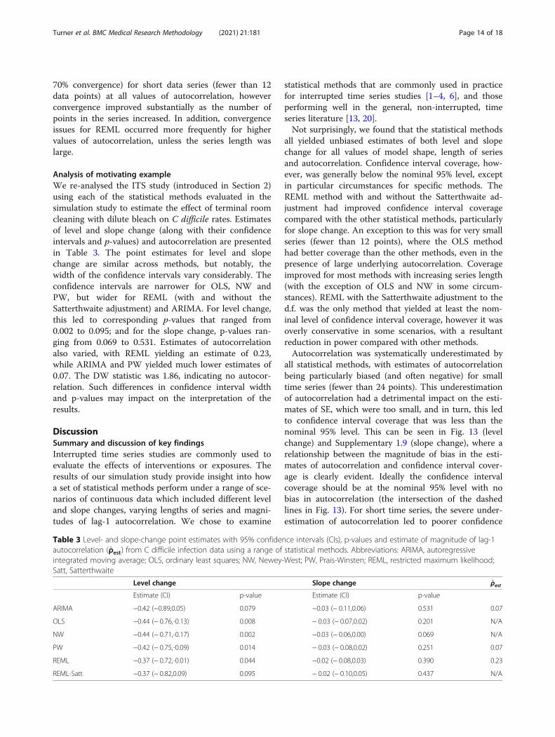
Analysis of motivating exampleWe re-analysed the ITS study (introduced in Section 2)using each of the statistical methods evaluated in thesimulation study to estimate the effect of terminal roomcleaning with dilute bleach on C difficile rates. Estimatesof level and slope change (along with their confidenceintervals and p-values) and autocorrelation are presentedin Table 3. The point estimates for level and slopechange are similar across methods, but notably, thewidth of the confidence intervals vary considerably. Theconfidence intervals are narrower for OLS, NW andPW, but wider for REML (with and without theSatterthwaite adjustment) and ARIMA. For level change,this led to corresponding p-values that ranged from0.002 to 0.095; and for the slope change, p-values ran-ging from 0.069 to 0.531. Estimates of autocorrelationalso varied, with REML yielding an estimate of 0.23,while ARIMA and PW yielded much lower estimates of0.07. The DW statistic was 1.86, indicating no autocor-relation. Such differences in confidence interval widthand p-values may impact on the interpretation of theresults.

DiscussionSummary and discussion of key findingsInterrupted time series studies are commonly used toevaluate the effects of interventions or exposures. Theresults of our simulation study provide insight into howa set of statistical methods perform under a range of sce-narios of continuous data which included different leveland slope changes, varying lengths of series and magni-tudes of lag-1 autocorrelation. We chose to examine

statistical methods that are commonly used in practicefor interrupted time series studies [1–4, 6], and thoseperforming well in the general, non-interrupted, timeseries literature [13, 20].Not surprisingly, we found that the statistical methods

all yielded unbiased estimates of both level and slopechange for all values of model shape, length of seriesand autocorrelation. Confidence interval coverage, how-ever, was generally below the nominal 95% level, exceptin particular circumstances for specific methods. TheREML method with and without the Satterthwaite ad-justment had improved confidence interval coveragecompared with the other statistical methods, particularlyfor slope change. An exception to this was for very smallseries (fewer than 12 points), where the OLS methodhad better coverage than the other methods, even in thepresence of large underlying autocorrelation. Coverageimproved for most methods with increasing series length(with the exception of OLS and NW in some circum-stances). REML with the Satterthwaite adjustment to thed.f. was the only method that yielded at least the nom-inal level of confidence interval coverage, however it wasoverly conservative in some scenarios, with a resultantreduction in power compared with other methods.Autocorrelation was systematically underestimated by

all statistical methods, with estimates of autocorrelationbeing particularly biased (and often negative) for smalltime series (fewer than 24 points). This underestimationof autocorrelation had a detrimental impact on the esti-mates of SE, which were too small, and in turn, this ledto confidence interval coverage that was less than thenominal 95% level. This can be seen in Fig. 13 (levelchange) and Supplementary 1.9 (slope change), where arelationship between the magnitude of bias in the esti-mates of autocorrelation and confidence interval cover-age is clearly evident. Ideally the confidence intervalcoverage should be at the nominal 95% level with nobias in autocorrelation (the intersection of the dashedlines in Fig. 13). For short time series, the severe under-estimation of autocorrelation led to poorer confidence

Table 3 Level- and slope-change point estimates with 95% confidence intervals (CIs), p-values and estimate of magnitude of lag-1autocorrelation (ρ̂est) from C difficile infection data using a range of statistical methods. Abbreviations: ARIMA, autoregressiveintegrated moving average; OLS, ordinary least squares; NW, Newey-West; PW, Prais-Winsten; REML, restricted maximum likelihood;Satt, Satterthwaite

Level change Slope change ρ̂estEstimate (CI) p-value Estimate (CI) p-value

ARIMA −0.42 (−0.89,0.05) 0.079 −0.03 (− 0.11,0.06) 0.531 0.07

OLS −0.44 (− 0.76,-0.13) 0.008 − 0.03 (− 0.07,0.02) 0.201 N/A

NW −0.44 (− 0.71,-0.17) 0.002 −0.03 (− 0.06,0.00) 0.069 N/A

PW −0.42 (− 0.75,-0.09) 0.014 − 0.03 (− 0.08,0.02) 0.251 0.07

REML −0.37 (− 0.72,-0.01) 0.044 −0.02 (− 0.08,0.03) 0.390 0.23

REML-Satt −0.37 (− 0.82,0.09) 0.095 − 0.02 (− 0.10,0.05) 0.437 N/A

Turner et al. BMC Medical Research Methodology (2021) 21:181 Page 14 of 18

interval coverage than had autocorrelation been ignored,as is the case with OLS.We included REML due to its potential to reduce bias

in the variance parameters compared with maximumlikelihood. Although the ARIMA model fitted in oursimulations used maximum likelihood estimation, themodel-based SEs were generally more similar to the em-pirical SEs for the ARIMA method compared with theREML method (where the model-based SEs were gener-ally smaller than the empirical SEs). ARIMA confidenceinterval coverage was similar to REML for level change,though REML showed improved confidence intervalcoverage for slope change. Further, the REML methodyielded less biased estimates of autocorrelation than theother methods, even for small series lengths.The only method to yield overly conservative confi-

dence intervals was the REML with SW adjustment to

the t-distribution d.f.. When deciding whether to use theSatterthwaite adjustment, consideration therefore needsto be made between the trade-off in the risk of type Iand type II errors. A further issue we identified with theSatterthwaite adjustment was that the adjusted d.f. werevery small in some series, leading to nonsensible confi-dence intervals. To limit this issue we set a minimumvalue of 2 for the d.f., but other choices could beadopted.The DW test is the most commonly used test to identify

autocorrelation and is often used when series are short [4,6]. Some authors use the test as part of a two-stage analysisstrategy where they first test for autocorrelation, and de-pending on the result of the test, either use a method thatattempts to adjust for autocorrelation or not. This type oftwo-stage approach is used in other contexts, such as test-ing for carryover in crossover trials. The findings of our

Fig. 13 Bias in autocorrelation estimate versus coverage for level change. The horizontal axis shows the bias in the autocorrelation estimate. Thevertical axis shows the percentage coverage. The horizontal dashed line indicates 95% coverage, the vertical dashed line indicates no bias in theestimate of autocorrelation. Each colour represents a different value of underlying autocorrelation, ranging from zero (purple) to 0.8 (red), witheach value displayed in a circle at the smallest series length (six points). The arrows point from shortest to longest series length, with the smallcircles at the end of each line showing coverage at a series length of 100 data points. Each data point shows the mean value from 10,000simulations for a given combination of autocorrelation coefficient and number of points in the series. The simulation combination presented isfor a level change of 2 and slope change of 0.1; however, other combinations give similar results. Abbreviations: ARIMA, autoregressive integratedmoving average; OLS, ordinary least squares; NW, Newey-West; PW, Prais-Winsten; REML, restricted maximum likelihood; Satt, Satterthwaite

Turner et al. BMC Medical Research Methodology (2021) 21:181 Page 15 of 18

simulation study underscore why such two stage ap-proaches fail and are discouraged; namely, due to their fail-ure to detect the presence of a statistic when it exists (i.e.,their high type II error rate). In our case, we found that forshort series (fewer than 12 data points), the DW test failedto identify autocorrelation when it was present, and formoderate length series (i.e. 48 points), with an underlyingautocorrelation of 0.2, autocorrelation was only detected in7% of the simulations. Other tests for autocorrelation areavailable [15, 36–39], though they are not commonly usedin practice [4, 6], and have been shown (through numericalsimulation) to have low power for short series [11, 15].

Comparisons with other studiesOur findings align with previous simulation studiesexamining the performance of statistical methods forITS. Huitema and McKean [40] similarly found thatOLS confidence interval coverage decreased with in-creasing series length (with six lengths ranging from 12to 500) in the presence of autocorrelation. McKnightet al. [14] similarly found that PW and ARIMA yieldedliberal Type I error rates for the regression modelparameters.Other simulation studies have investigated the per-

formance of methods for general time series, and ourfindings also align with these. Alpargu and Dutilleul [13]concluded from their simulation study examining theperformance of REML, PW and OLS for lag (1) timeseries data over a range of series lengths (from 10 to200), that REML is to be preferred over OLS and PW inestimating slope parameters. Cheang and Reinsel [20]examined the performance of ML and REML for esti-mating linear trends in lag (1) time series data of length60 and 120 (both with and without seasonal compo-nents) and concluded that the REML estimator yieldedbetter confidence interval coverage for the slope param-eter, and less biased estimates of autocorrelation. Smithand McAleer [12] examined the performance of the NWestimator for time series of length 100 with lags of 1, 3and 10, and found that it underestimated the SEs of theslope parameter.

Strengths and limitationsThe strengths of our study include that we have usedmany combinations of parameter estimates and statis-tical methods. Our parameter values were informed bycharacteristics of real world ITS studies [4]. We plannedand reported our study using the structured approach ofMorris et al. [32] for simulation studies, and we gener-ated a large number of data sets per combination tominimise MCSE.As with all simulation studies, there are limitations to

the applicability of findings. All data series were basedon a random number generator and results may change

given a different set of series, however, this is unlikely tobe problematic given our MCSE was < 0.5% for all po-tential values of coverage and type I error rate. Our find-ings are only applicable to the scenarios in which theywere generated, and so may not apply to ITS studieswith different characteristics, such as unequal numbersof time points in the pre- and post-interruptionsegments, non-constant variance or different lags ofautocorrelation (including seasonal effects).

Implications for practiceWe found that all methods yielded unbiased estimates ofthe level and slope change, however, the methods dif-fered in their performance in terms of confidence inter-val coverage and estimation of the autocorrelationparameter. Confidence interval coverage was primarilydetermined by the length of the time series and theunderlying magnitude of autocorrelation. In practice,however, most analysts will only have knowledge of thelength of the time series to guide in the choice ofmethod. In rare cases, knowledge of the likely size of theunderlying autocorrelation may be available from a pre-vious long time series study in a similar context, whichcould help inform their choice. In our review of ITSstudies investigating public health interruptions or expo-sures, the magnitude of autocorrelation was almostnever explicitly specified (1%, 3/230 time series) [4].Analysis of data extracted from the ITS studies includedin this review using the REML method yielded a medianautocorrelation 0.2 (IQR: 0 to 0.6, n = 180); however, asshown from the simulation study, the estimates of auto-correlation (on which these summary statistics arebased) are likely to be underestimated.From the statistical methods and scenarios we exam-

ined, we found that for small time series (approximately12 points or under), in the absence of a method thatperforms well adjusting for autocorrelation in such shortseries, OLS is the recommended method. For longertime series, REML is recommended. If the analyst hasknowledge that the underlying autocorrelation is likelyto be large, then using REML with the Satterthwaite ad-justment may be advantageous. However, when the Sat-terthwaite adjustment yields d.f. lower than 2, werecommend replacing these with 2 to mitigate nonsensi-ble confidence intervals. When REML doesn’t converge,ARIMA provides a reasonable alternative as, with the ex-ception of REML, it yields higher confidence intervalcoverage than the other methods. Given most methodswill yield confidence intervals that are too small, withtype I error rates greater than 5%, borderline findings ofstatistical significance for the regression parametersshould be cautiously interpreted; these may be due tochance rather than as a result of the interruption.

Turner et al. BMC Medical Research Methodology (2021) 21:181 Page 16 of 18

Estimates of autocorrelation from long series can beuseful to inform sample size calculations and analyticaldecisions in future studies. We recommend reportingthe REML estimates of the autocorrelation coefficientwhen possible. We only recommend using the DW testfor detecting underlying autocorrelation in long timeseries (longer than 100 data points) and recommendagainst its use as part of a two-stage or stepwise ap-proach to determine whether to use a statistical methodthat adjusts for autocorrelation.In terms of study design, we recommend using 24 data

points at the very minimum. With this number of points,confidence interval coverage close to the nominal 95%level can be achieved using REML with the Satterthwaiteadjustment (when underlying autocorrelation is between 0and 0.6). With fewer data points, poor confidence intervalcoverage is likely, irrespective of method.

Implications for future researchAlthough we investigated the statistical methods mostcommonly observed in reviews of ITS studies [1–4, 6],there is scope for further research examining other statis-tical methods, such as robust methods [41] or Bayesianapproaches where the uncertainty in the estimate of auto-correlation could be incorporated. We investigated onesmall-sample adjustment (Satterthwaite) though others,such as Kenward-Roger [42], which adds a correction tothe SE of regression parameter estimates, could also beexamined. Further investigation of how the methodsperform for scenarios other than those we investigatedwould be valuable. For example, when there are unequalnumbers of points pre- and post-interruption, lags greaterthan 1, and where the autocorrelation and error variancediffer between the pre and post interruption periods.

ConclusionWe undertook a simulation study to examine the per-formance of a set of statistical methods to analyse con-tinuous ITS data under a range of scenarios thatincluded different level and slope changes, varyinglengths of series and magnitudes of lag-1 autocorrel-ation. We found that all methods yielded unbiased esti-mates of the level and slope change, however, themagnitude of autocorrelation was underestimated by allmethods. This generally led to SEs that were too smalland confidence interval coverage that was less than thenominal level. The DW test for the presence of autocor-relation performed poorly except for long series andlarge underlying autocorrelation. Care is needed wheninterpreting results from all methods, given the confi-dence intervals will generally be too narrow. Furtherresearch is required to determine and develop methodsthat perform well in the presence of autocorrelation,especially for short series.

AbbreviationsARIMA: Autoregressive integrated moving average; ARMAX: Autoregressivemoving average exogeneous; CI: Confidence interval; CO: Cochrane-orcutt;d.f.: Degrees of freedom; DW: Durbin-Watson; GLS: Generalised least squares;HAI: Healthcare-associated infection; IQR: Inter-quartile range; ITS: Interruptedtime series; OLS: Ordinary least squares; MCSE: Monte-Carlo standard error;NHMRC: National health and medical research council; NW: Newey-west;PW: Prais-winsten; REML: Restricted maximum likelihood; Satt: Sattherthwaite;SD: Standard deviation; SE: Standard error

Supplementary InformationThe online version contains supplementary material available at https://doi.org/10.1186/s12874-021-01364-0.

Additional file 1: Appendices This file contains the appendicesreferenced in the text. STurner_ITS_Simulation_Appendices.docx

Additional file 2: Supplementary File 1 This file contains thesupplementary graphs described in the text..STurner_ITS_Simulation_Supplementary_File_1.docx

AcknowledgementsThis work forms part of SLT’s PhD, which is supported by an AustralianPostgraduate Award administered through Monash University, Australia.

Authors’ contributionsJEM and ABF conceived the study and all authors contributed to its design.SLT designed and wrote the computer code and ran and analysed thesimulations. SLT wrote the first draft of the manuscript, with contributionsfrom JEM. SLT, JEM, AK, ABF, MT contributed to revisions of the manuscriptand take public responsibility for its content.

FundingThis work was supported by the Australian National Health and MedicalResearch Council (NHMRC) project grant (1145273). SLT was funded throughan Australian Postgraduate Award administered through Monash University,Australia. JEM is supported by an NHMRC Career Development Fellowship(1143429). The funders had no role in study design, decision to publish, orpreparation of the manuscript.

Availability of data and materialsThe data and computer code used to analyse the motivating example, thecomputer code used to create and analyse the simulated data sets, and thecomputer code used to plot the graphs in the manuscript (includingSupplementary File 1) are available in the figshare repository, https://doi.org/10.26180/13284329 [33].

Declarations

Ethics approval and consent to participateNot applicable.

Consent for publicationNot applicable.

Competing interestsThe authors declare that they have no competing interests.

Author details1School of Public Health and Preventive Medicine, Monash University, 533 StKilda Road, Melbourne, Victoria, Australia. 2Clinical Epidemiology Program,Ottawa Hospital Research Institute, Carling Ave, Ottawa, Ontario 1053,Canada. 3School of Epidemiology, Public Health and Preventive Medicine,University of Ottawa, Laurier Ave E, Ottawa, Ontario 75, Canada.

Turner et al. BMC Medical Research Methodology (2021) 21:181 Page 17 of 18

Received: 8 December 2020 Accepted: 21 July 2021

References1. Ramsay CR, Matowe L, Grilli R, Grimshaw JM, Thomas RE. Interrupted time

series designs in health technology assessment: lessons from twosystematic reviews of behavior change strategies. Int J Technol AssessHealth Care. 2003;19(4):613–23. https://doi.org/10.1017/S0266462303000576.

2. Jandoc R, Burden AM, Mamdani M, Lévesque LE, Cadarette SM. Interruptedtime series analysis in drug utilization research is increasing: systematicreview and recommendations. J Clin Epidemiol. 2015;68(8):950–6. https://doi.org/10.1016/j.jclinepi.2014.12.018.

3. Ewusie J, Soobiah C, Blondal E, Beyene J, Thabane L, Hamid J. Methods,applications and challenges in the analysis of interrupted time series data: ascoping review. J Multidiscip Healthc. 2020;13:411–23. https://doi.org/10.2147/JMDH.S241085.

4. Turner SL, Karahalios A, Forbes AB, Taljaard M, Grimshaw JM, Cheng AC,et al. Design characteristics and statistical methods used in interrupted timeseries studies evaluating public health interventions: a review. J ClinEpidemiol. 2020;122:1–11. https://doi.org/10.1016/j.jclinepi.2020.02.006.

5. Wagner AK, Soumerai SB, Zhang F, Ross-Degnan D. Segmented regressionanalysis of interrupted time series studies in medication use research. J ClinPharm Ther. 2002;27(4):299–309. https://doi.org/10.1046/j.1365-2710.2002.00430.x.

6. Hudson J, Fielding S, Ramsay CR. Methodology and reporting characteristicsof studies using interrupted time series design in healthcare. BMC Med ResMethodol. 2019;19(1):137. https://doi.org/10.1186/s12874-019-0777-x.

7. Kontopantelis E, Doran T, Springate DA, Buchan I, Reeves D. Regressionbased quasi-experimental approach when randomisation is not an option:interrupted time series analysis. BMJ Br Med J. 2015;350(jun09 5):h2750.https://doi.org/10.1136/bmj.h2750.

8. Lopez Bernal J, Cummins S, Gasparrini A. Interrupted time series regressionfor the evaluation of public health interventions: a tutorial. Int J Epidemiol.2016:dyw098.

9. Penfold RB, Zhang F. Use of interrupted time series analysis in evaluatinghealth care quality improvements. Acad Pediatr. 2013;13(6):S38–44. https://doi.org/10.1016/j.acap.2013.08.002.

10. Gebski V, Ellingson K, Edwards J, Jernigan J, Kleinbaum D. Modellinginterrupted time series to evaluate prevention and control of infection inhealthcare. Epidemiol Infect. 2012;140(12):2131–41. https://doi.org/10.1017/S0950268812000179.

11. Huitema BE, McKean JW. Identifying autocorrelation generated by variouserror processes in interrupted time-series regression designs. Educ PsycholMeas. 2007;67(3):447–59. https://doi.org/10.1177/0013164406294774.

12. Smith J, McAleer M. Newey-West covariance matrix estimates for modelswith generated regressors. Appl Econ. 1994;26(6):635–40. https://doi.org/10.1080/00036849400000034.

13. Alpargu G, Dutilleul P. Efficiency and validity analyses of two-stageestimation procedures and derived testing procedures in quantitative linearmodels with AR(1) errors. Commun Stat Simul Comput. 2003;32(3):799–833.https://doi.org/10.1081/SAC-120017863.

14. McKnight SD, McKean JW, Huitema BE. A double bootstrap method toanalyze linear models with autoregressive error terms. Psychol Methods.2000;5(1):87–101. https://doi.org/10.1037/1082-989X.5.1.87.

15. Huitema BE, McKean JW. An improved portmanteau test for autocorrelatederrors in interrupted time-series regression models. Behav Res Methods.2007;39(3):343–9. https://doi.org/10.3758/BF03193002.

16. Brennan SE, McDonald, S., Cheng, A., Reid, J., Allen, K., McKenzie, J.E.Systematic review of novel disinfection methods to reduce infection ratesin high risk hospitalised populations. Monash University, Melbourne,Australia.: Prepared by Cochrane Australia for the National Health andMedical Research Council. ; 2017.

17. Hacek DM, Ogle AM, Fisher A, Robicsek A, Peterson LR. Significant impact ofterminal room cleaning with bleach on reducing nosocomial Clostridiumdifficile. Am J Infect Control. 2010;38(5):350–3. https://doi.org/10.1016/j.ajic.2009.11.003.

18. Huitema BE. Analysis of covariance and alternatives statistical methods forexperiments, quasi-experiments, and single-case studies. 2nd ed. Hoboken,N.J: Wiley; 2011.

19. Huitema BE, Mckean JW. Design specification issues in time-seriesintervention models. Educ Psychol Meas. 2000;60(1):38–58. https://doi.org/10.1177/00131640021970358.

20. Cheang W-K, Reinsel GC. Bias reduction of autoregressive estimates in timeseries regression model through restricted maximum likelihood. J Am StatAssoc. 2000;95(452):1173–84. https://doi.org/10.1080/01621459.2000.10474318.

21. Kutner M, Nachtscheim C, Neter J, Li W, Senter H. Applied linear statisticalmodels. In: Kutner M, Nachtscheim C, Neter J, Li W, Senter H, editors. 2008.p. 880-.

22. Newey WK, West KD. A simple, positive semi-definite, heteroskedasticity andautocorrelation consistent covariance matrix. Econometrica. 1987;55(3):703.https://doi.org/10.2307/1913610.

23. StataCorp. Stata 15 Base Reference Manual. College Station, TX: Stata Press;2017.

24. Singer J, Willett J. Applied longitudinal data analysis: modeling change andevent occurrence 2003. xx-xx p.

25. Thompson WA. The problem of negative estimates of variancecomponents. Ann Math Stat. 1962;33(1):273–89. https://doi.org/10.1214/aoms/1177704731.

26. Satterthwaite FE. An approximate distribution of estimates of variancecomponents. Biom Bull. 1946;2(6):110–4. https://doi.org/10.2307/3002019.

27. Paolella MS. Linear models and time-series analysis : regression, ANOVA,ARMA and GARCH. Hoboken, NJ: John Wiley & Sons, Inc; 2019.

28. Turner SL, Karahalios A, Forbes AB, Taljaard M, Grimshaw JM, McKenzie JE.Comparison of six statistical methods for interrupted time series studies:empirical evaluation of 190 published series. BMC Med Res Methodol. 2021;21(1):134. https://doi.org/10.1186/s12874-021-01306-w.

29. Nelson BK. Statistical methodology: V. Time series analysis usingautoregressive integrated moving average (ARIMA) models. Acad EmergMed. 1998;5(7):739.

30. Box GEPa. Time series analysis : forecasting and control. 5th ed: Hoboken,New Jersey : Wiley; 2016.

31. Durbin J, Watson GS. Testing for serial correlation in least squaresregression: I. Biometrika. 1950;37(3/4):409–28.

32. Morris TP, White IR, Crowther MJ. Using simulation studies to evaluatestatistical methods. Stat Med. 2019;38(11):2074–102. https://doi.org/10.1002/sim.8086.

33. Turner SL, Forbes AB, Karahalios A, Taljaard M, McKenzie JE. Evaluation ofstatistical methods used in the analysis of interrupted time series studies: asimulation study - code and data 2020.

34. White IR. Simsum: analyses of simulation studies including Monte Carloerror. Stata J. 2010;10:369.

35. Stata. Stata Statistical Software, vol. 15. College Station, TX: Statcorp LLC; 2017.36. Box GEP, Pierce DA. Distribution of residual autocorrelations in

autoregressive-integrated moving average time series models. J Am StatAssoc. 1970;65(332):1509–26. https://doi.org/10.1080/01621459.1970.10481180.

37. Ljung GM, Box GEP. On a measure of lack of fit in time series models.Biometrika. 1978;65(2):297–303. https://doi.org/10.1093/biomet/65.2.297.

38. Breusch TS. Testing for autocorrelation in dynamic linear models. Aust EconPap. 1978;17(31):334–55. https://doi.org/10.1111/j.1467-8454.1978.tb00635.x.

39. Godfrey LG. Testing against general autoregressive and moving averageerror models when the Regressors include lagged dependent variables.Econometrica. 1978;46(6):1293–301. https://doi.org/10.2307/1913829.

40. Huitema BE, McKean JW, McKnight S. Autocorrelation effects on least-squares intervention analysis of short time series. Educ Psychol Meas. 1999;59(5):767–86. https://doi.org/10.1177/00131649921970134.

41. Cruz M, Bender M, Ombao H. A robust interrupted time series model foranalyzing complex health care intervention data. Stat Med. 2017;36(29):4660–76. https://doi.org/10.1002/sim.7443.

42. Kenward MG, Roger JH. Small sample inference for fixed effects fromrestricted maximum likelihood. Biometrics. 1997;53(3):983–97. https://doi.org/10.2307/2533558.

Publisher’s NoteSpringer Nature remains neutral with regard to jurisdictional claims inpublished maps and institutional affiliations.

Turner et al. BMC Medical Research Methodology (2021) 21:181 Page 18 of 18