Evaluation of LS-DYNAWood Material Model 143

PUBLICATION NO. FHWA-HRT-04-096 AUGUST 2005

Research, Development, and TechnologyTurner-Fairbank Highway Research Center6300 Georgetown PikeMcLean, VA 22101-2296

Foreword

This report documents the evaluation of a wood material model that has been implemented into the dynamic finite element code LS-DYNA, beginning with version 970. This material model was developed specifically to predict the dynamic performance of wood components used in roadside safety structures when undergoing a collision by a motor vehicle. This model is applicable for all varieties of wood when appropriate material coefficients are inserted. Default material coefficients for two wood varieties, southern yellow pine and Douglas fir, are stored in the model and can be accessed for use. This report is one of two that completely documents this material model. The first report, Manual for LS-DYNA Wood Material Model 143 (FHWA-HRT-04-097), completely documents this material model for the user. The second report, Evaluation of LS-DYNA Wood Material Model 143 (FHWA-HRT-04-096), completely documents the model’s performance and the accuracy of the results. This performance evaluation was a collaboration between the model developer and the model evaluator. Regarding the model’s performance evaluation, the developer and the evaluator were unable to come to a final agreement regarding the model’s performance and accuracy. These disagreements are itemized and thoroughly discussed in chapter 17 of the second report. This report will be of interest to research engineers associated with the evaluation and crashworthy performance of roadside safety structures, particularly those engineers responsible for the prediction of the crash response of such structures when using the finite element code LS-DYNA.

Michael F. Trentacoste Director, Office of Safety Research and Development

Notice This document is disseminated under the sponsorship of the U.S. Department of Transportation in the interest of information exchange. The U.S. Government assumes no liability for its contents or use thereof. This report does not constitute a standard, specification, or regulation. The U.S. Government does not endorse products or manufacturers. Trade and manufacturers’ names appear in this report only because they are considered essential to the object of the document.

Quality Assurance Statement

The Federal Highway Administration (FHWA) provides high-quality information to serve Government, industry, and the public in a manner that promotes public understanding. Standards and policies are used to ensure and maximize the quality, objectivity, utility, and integrity of its information. FHWA periodically reviews quality issues and adjusts its programs and processes to ensure continuous quality improvement.

Technical Report Documentation Page 1. Report No.

FHWA-HRT-04-096

2. Government Accession No.

3. Recipient’s Catalog No. 5. Report Date August 2005

4. Title and Subtitle

Evaluation of LS-DYNA Wood Material Model 143 6. Performing Organization Code

7. Author(s)

Y.D. Murray, J.D. Reid, R.K. Faller, B.W. Bielenberg, and T.J. Paulsen

8. Performing Organization Report No.

9. Performing Organization Name and Address APTEK, Inc. 1257 Lake Plaza Drive, Suite 100 Colorado Springs, CO 80906-3558

10. Work Unit No. (TRAIS)

Midwest Roadside Safety Facility University of Nebraska at Lincoln 1901 Y Street, Building C Lincoln, NE 68588-0601

11. Contract or Grant No.

DTFH61-98-C-00071

13. Type of Report and Period Covered Final Report Sept. 1998-Sept. 2002

12. Sponsoring Agency’s Name and Address Volpe National Transportation Systems Center 55 Broadway, Kendall Square Cambridge, MA 02142-1093 Federal Highway Administration 6300 Georgetown Pike McLean, VA 22101-2296

14. Sponsoring Agency’s Code

15. Supplementary Notes

Contracting Officer’s Technical Representative (COTR): Martin Hargrave, Office of Safety Research and Development 16. Abstract

Calculations are performed with the finite element code LS-DYNA to evaluate the performance of wood material model 143 and to set default material properties for southern yellow pine and Douglas fir. Correlations with published test data include static bending and compression simulations of dry timbers, static bending of saturated posts, and dynamic simulation of saturated posts impacted by bogie vehicles. The companion manual to this report is: Manual for LS-DYNA Wood Material Model 143 (FHWA-HRT-04-097)

17. Key Words Wood, southern yellow pine, Douglas fir, LS-DYNA, modeling and simulation, damage, rate effects, plasticity.

18. Distribution Statement No restrictions. This document is available to the public through the National Technical Information Service, Springfield, VA 22161.

19. Security Classif. (of this report)

Unclassified

20. Security Classif. (of this page)

Unclassified

21. No. of Pages

152

22. Price

Form DOT F 1700.7 (8-72) Reproduction of completed page authorized

ii

Preface The goal of the work performed under this program, Development of DYNA3D Analysis Tools for Roadside Safety Applications, is to develop wood and soil material models, implement the models into the LS-DYNA finite element code,(1) and evaluate the performance of each model through correlations with available test data. Two reports are available for each material model. One report is a user’s manual; the second report is a performance evaluation. The user’s manual, Manual for LS-DYNA Wood Material Model 143,(2) thoroughly documents the wood model theory, reviews the model input, and provides example problems for use as a learning tool. It is written by the developer of the model. This report, Evaluation of LS-DYNA Wood Material Model 143, comprises the performance evaluation for the wood model. It documents LS-DYNA parametric studies and correlations with test data performed by the model developer, and by a potential end user. The reader is urged to review the user’s manual before reading this evaluation report. A user’s manual(3) and evaluation report(4) are also available for the soil model. The development of the wood model was conducted by the prime contractor. The associated wood model evaluation effort to determine the model‘s performance and the accuracy of the results was a collaboration between the developer and the potential end user, with the user’s evaluation intended to be independent of the developer’s evaluation. The developer partially evaluated the wood model. The potential end user performed a second independent evaluation of the wood model, provided finite element meshes for the evaluation calculations, and provided static post and bogie impact test data for correlations with the model. Regarding the second independent evaluation of the wood model, the developer and evaluator were unable to come to a final agreement regarding several issues associated with the model‘s performance and accuracy. These issues are itemized and thoroughly discussed by the developer in chapter 17 of this evaluation report. Throughout this report, the developer of the wood material model is referred to as the developer. The potential end user of the wood material model is referred to as the user. The developer’s calculations and conclusions are given in chapters 1 through 8 of this report. The user’s calculations and conclusions are given in chapters 9 through 16 of this report.

iii

SI* (MODERN METRIC) CONVERSION FACTORS APPROXIMATE CONVERSIONS TO SI UNITS

Symbol When You Know Multiply By To Find Symbol LENGTH

in inches 25.4 millimeters mm ft feet 0.305 meters m yd yards 0.914 meters m mi miles 1.61 kilometers km

AREA in2 square inches 645.2 square millimeters mm2

ft2 square feet 0.093 square meters m2

yd2 square yard 0.836 square meters m2

ac acres 0.405 hectares ha mi2 square miles 2.59 square kilometers km2

VOLUME fl oz fluid ounces 29.57 milliliters mL gal gallons 3.785 liters L ft3 cubic feet 0.028 cubic meters m3

yd3 cubic yards 0.765 cubic meters m3

NOTE: volumes greater than 1000 L shall be shown in m3

MASS oz ounces 28.35 grams glb pounds 0.454 kilograms kgT short tons (2000 lb) 0.907 megagrams (or "metric ton") Mg (or "t")

TEMPERATURE (exact degrees) oF Fahrenheit 5 (F-32)/9 Celsius oC

or (F-32)/1.8 ILLUMINATION

fc foot-candles 10.76 lux lx fl foot-Lamberts 3.426 candela/m2 cd/m2

FORCE and PRESSURE or STRESS lbf poundforce 4.45 newtons N lbf/in2 poundforce per square inch 6.89 kilopascals kPa

APPROXIMATE CONVERSIONS FROM SI UNITS Symbol When You Know Multiply By To Find Symbol

LENGTHmm millimeters 0.039 inches in m meters 3.28 feet ft m meters 1.09 yards yd km kilometers 0.621 miles mi

AREA mm2 square millimeters 0.0016 square inches in2

m2 square meters 10.764 square feet ft2

m2 square meters 1.195 square yards yd2

ha hectares 2.47 acres ac km2 square kilometers 0.386 square miles mi2

VOLUME mL milliliters 0.034 fluid ounces fl oz L liters 0.264 gallons gal m3 cubic meters 35.314 cubic feet ft3

m3 cubic meters 1.307 cubic yards yd3

MASS g grams 0.035 ounces ozkg kilograms 2.202 pounds lbMg (or "t") megagrams (or "metric ton") 1.103 short tons (2000 lb) T

TEMPERATURE (exact degrees) oC Celsius 1.8C+32 Fahrenheit oF

ILLUMINATION lx lux 0.0929 foot-candles fc cd/m2 candela/m2 0.2919 foot-Lamberts fl

FORCE and PRESSURE or STRESS N newtons 0.225 poundforce lbf kPa kilopascals 0.145 poundforce per square inch lbf/in2

*SI is the symbol for th International System of Units. Appropriate rounding should be made to comply with Section 4 of ASTM E380. e(Revised March 2003)

iv

Table of Contents

1 DEVELOPER’S INTRODUCTION........................................................................ 1

1.1 MODEL THEORY ...................................................................................... 1 1.2 MODEL INPUT .......................................................................................... 1 1.3 LIMITATIONS OF LABORATORY MATERIAL PROPERTY DATA........... 3 1.4 EVALUATION PROCESS.......................................................................... 3 1.5 VERIFICATION AND VALIDATION........................................................... 4

2 SINGLE-ELEMENT SIMULATIONS .................................................................... 5 3 TIMBER COMPRESSION TEST CORRELATIONS ............................................ 7 4 TIMBER-BENDING TEST CORRELATIONS ...................................................... 9 5 QUASI-STATIC POST TEST CORRELATIONS................................................ 11

5.1 SOUTHERN YELLOW PINE BENDING TEST DATA ............................. 11 5.2 LS-DYNA CORRELATIONS .................................................................... 16 5.3 LS-DYNA PARAMETRIC STUDIES ........................................................ 21

6 DYNAMIC POST TEST CORRELATIONS ........................................................ 31

6.1 BOGIE IMPACT TEST DATA .................................................................. 31 6.2 LS-DYNA CORRELATIONS .................................................................... 34 6.3 FILTERING AND SAMPLING ISSUES.................................................... 38 6.4 LS-DYNA PARAMETRIC STUDIES ........................................................ 43

7 ADDITIONAL EVALUATION CALCULATIONS................................................ 47

7.1 PLASTICITY ALGORITHM ITERATIONS................................................ 47 7.2 FULLY INTEGRATED ELEMENTS ......................................................... 48 7.3 EROSION CRITERIA............................................................................... 50 7.4 POST-PEAK HARDENING PARAMETER............................................... 53

8 DEVELOPER’S SUMMARY AND RECOMMENDATIONS................................ 57 9 USER’S INTRODUCTION.................................................................................. 63 10 VALIDATION CRITERIA FOR THE WOOD MATERIAL MODEL ..................... 65

10.1 NDOR TESTS: PERFORMANCE ENVELOPES ..................................... 65 11 VERIFICATION OF RESULTS ON DIFFERENT COMPUTER PLATFORMS... 71

11.1 SINGLE-ELEMENT MODELS ................................................................. 71 11.2 DYNAMIC POST TEST SIMULATION: BOGIE MODEL.......................... 73 11.3 DYNAMIC POST TEST SIMULATION: FAST BOGIE MODEL ............... 76

12 SINGLE ELEMENT: TENSION PARALLEL TO THE GRAIN ........................... 79 12.1 STRESS-STRAIN BEHAVIOR: *MAT_WOOD_PINE.............................. 80

v

12.2 VOLUME OF ELEMENT: *MAT_WOOD_PINE ....................................... 81 12.3 MATERIAL PROPERTIES: *MAT_WOOD_PINE .................................... 82

13 STATIC WOOD POST TEST SIMULATIONS.................................................... 85

13.1 STATIC POST MODEL............................................................................ 85 13.2 BASELINE MODEL VERSUS TEST COMPARISON .............................. 87 13.3 BASELINE VERSUS REFINED-MESH COMPARISON.......................... 88 13.4 PARAMETER STUDY ............................................................................. 90

14 DYNAMIC WOOD POST TEST SIMULATIONS................................................ 95

14.1 DYNAMIC POST MODEL........................................................................ 95 14.2 VAPORIZATION AND TIME STEP.......................................................... 96 14.3 SHARP EDGE CONTACTS..................................................................... 97 14.4 BENDING ................................................................................................ 98 14.5 FURTHER ANALYSIS ............................................................................. 99

15 ELEMENT FORMULATION: HOURGLASSING.............................................. 103 16 USER’S CONCLUSIONS................................................................................. 107 17 DEVELOPER’S COMMENTS ON USER’S EVALUATION ............................. 109

17.1 TABLE OF WOOD MODEL TOPICS..................................................... 111 17.2 DISCUSSION OF WOOD MODEL TOPICS.......................................... 113 17.3 INSTABILITIES IN DYNAMIC ANALYSES............................................ 123

18 REFERENCES................................................................................................. 141

vi

List of Figures Figure 1. LS-DYNA simulations of southern yellow pine showing brittle behavior in

tension and shear, and ductile behavior in compression.......................................... 2 Figure 2. Good correlation between LS-DYNA simulations (dashed lines) and measured

clear wood data (solid lines) for southern yellow pine in tension parallel to the grain.................................................................................................................................. 5

Figure 3. Good correlation between LS-DYNA simulations (dashed lines) and measured clear wood data (solid lines) for southern yellow pine in compression perpendicular to the grain ............................................................................................................... 6

Figure 4. Schematic of FPL timber compression test setup. ........................................... 7 Figure 5. These comparisons of the model with test data were used to set the hardening

behavior of the southern yellow pine model in parallel-to-the-grain compression. ... 8 Figure 6. These comparisons of the model with the parallel-to-the-grain timber-bending

test data demonstrate the need for different quality factors in tension and compression........................................................................................................... 10

Figure 7. Quasi-static post test setup. ........................................................................... 11 Figure 8. Details for the rigid frame used in the quasi-static post test setup. ................ 12 Figure 9. Deformed configurations of posts in static tests. ............................................ 13 Figure 10. Closeup of damage observed in break region of posts in static tests........... 13 Figure 11. Measured load-deflection histories exhibit sudden drops in force as the post

fails in the tensile region......................................................................................... 14 Figure 12. Quasi-static (blue solid line) and dynamic (pink dashed line) performance

envelopes developed and plotted by the user. ....................................................... 15 Figure 13. Grades 1 and 1D static post test measurements exhibit substantial scatter.16 Figure 14. Good correlations between the LS-DYNA calculations and quasi-static

performance envelopes determine the default quality factors for grade 1 southern yellow pine of QT = 0.47 with QC = 0.63. ................................................................ 18

Figure 15. Good correlations between the LS-DYNA calculations and quasi-static performance envelopes determine the default quality factors for DS-65 southern yellow pine of QT = 0.80 with QC = 0.93. ................................................................ 19

Figure 16. The parallel-to-the-grain post fracture calculated in the post just below the top of the rigid support is in agreement with the location of the damage observed in the tests. ................................................................................................................ 20

Figure 17. Three geometric models were set up for performing parametric calculations................................................................................................................................ 21

Figure 18. The force-deflection curve calculated with the fast-running, rigid-wall model is similar to that calculated with the full-support structure, making it useful for performing parametric calculations. ....................................................................... 22

Figure 19. Pinning a truss to the bolt to simulate the vertical force applied by the pulley system increases the peak force by about 4 percent. ............................................ 23

Figure 20. The peak force increases with the applied velocity until convergence is attained at 0.25 mm/ms.......................................................................................... 23

Figure 21. Quasi-static calculations are filtered for easier comparison with the unfiltered test data. ................................................................................................................ 24

vii

Figure 22. The energy required to break the post increases as the value of the parallel-to-the-grain fracture energy increases. .................................................................. 25

Figure 23. Calculations with QC > QT soften more rapidly than calculations with QC = QT................................................................................................................................ 25

Figure 24. The calculated peak force increases with increasing values of the softening parameter B. .......................................................................................................... 26

Figure 25. The softening parameter B determines the shape of the softening curve in these single-element simulations for tension parallel to the grain. ......................... 26

Figure 26. Type 4 stiffness control reduces hourglassing better than type 3 viscous control. ................................................................................................................... 28

Figure 27. The peak force calculated with type 4 stiffness control agrees with the fully integrated element calculation better than the type 3 viscous calculation. ............. 29

Figure 28. Less final hourglass energy is calculated with type 4 stiffness control than with type 3 viscous control. .................................................................................... 29

Figure 29. Decreasing the moisture content by 6 percent increases the post-peak force by 80 percent. ........................................................................................................ 30

Figure 30. Post setup for dynamic bogie impact tests. .................................................. 32 Figure 31. Processed data from the user’s bogie impact tests...................................... 33 Figure 32. Damage in the breakaway region of the posts, just below ground level. ...... 34 Figure 33. These correlations between the LS-DYNA calculations and the performance

envelopes were used to adjust the parallel fracture energy for grade 1 pine to 50 times the perpendicular fracture energy................................................................. 35

Figure 34. These correlations between the LS-DYNA calculations and the performance envelopes were used to adjust the parallel fracture energy for DS-65 pine to 85 times the perpendicular fracture energy................................................................. 35

Figure 35. These correlations between the LS-DYNA calculations and the energy-deflection data were used to confirm that grade 1 Douglas fir can be simulated with the same parallel fracture energy and rate-effect parameters as grade 1 southern yellow pine, but with different quality factors. ......................................................... 36

Figure 36. These correlations between the LS-DYNA calculations and the energy-deflection data were used to set the parallel fracture energy for frozen grade 1 pine to five times the perpendicular fracture energy. ..................................................... 36

Figure 37. The simulated post breaks just below ground level, in agreement with the failure location observed in the tests. ..................................................................... 38

Figure 38. User’s geometric bogie model used in the developer’s calculations............. 39 Figure 39. The filtered bogie acceleration history sampled at 3200 Hz is significantly

different than the history sampled at 10,000 Hz. .................................................... 40 Figure 40. Force-deflection histories calculated from bogie nodal accelerations depend

significantly on the bogie type and output sampling frequency. ............................. 41 Figure 41. Force-deflection histories calculated from the wood post cross-sectional

forces are not significantly affected by the details for the bogie model or sampling frequency. .............................................................................................................. 42

Figure 42. The internal energy calculated to break the wood post is less than the kinetic energy reduction of the bogie................................................................................. 43

viii

Figure 43. These deformed configurations at 180 mm of deflection indicate that adjustments in the quality factors affect the deflection at which the grade 1 pine post breaks in two. ................................................................................................. 45

Figure 44. Although the grade 1 pine post breaks earlier in time with QT = 0.40 and QC = 0.70, the calculated energy and velocity histories are similar. ....................... 45

Figure 45. The default number of plasticity algorithm iterations is set to one because these static load-deflection curves are insensitive to the number of iterations....... 47

Figure 46. Erosion affects the fully integrated element curves, but not the under-integrated element curves, indicating that the fully integrated elements erode while still carrying load. ................................................................................................... 48

Figure 47. Deformed configurations and fringes of damage calculated with fully integrated elements (eight points) are similar to those calculated with under-integrated elements (one point).............................................................................. 49

Figure 48. Energy-deflection and bogie velocity-reduction histories are not strongly influenced by the type of element formulation (eight points or one point) modeled in the breakaway region............................................................................................. 49

Figure 49. The breakaway region calculated with perpendicular erosion in these static bending simulations looks more realistic than that calculated without perpendicular erosion; however, perpendicular erosion is not recommended for practical use.... 51

Figure 50. Load-deflection curves calculated with perpendicular erosion are slightly more brittle than those calculated without perpendicular erosion........................... 51

Figure 51. The breakaway region calculated with perpendicular erosion in this bogie impact simulation looks more realistic than that calculated without perpendicular erosion. .................................................................................................................. 52

Figure 52. Dynamic load-deflection and bogie velocity-reduction curves calculated with perpendicular erosion are nearly identical to those calculated without perpendicular erosion. .................................................................................................................. 52

Figure 53. Use of perpendicular erosion causes excessive erosion to be calculated in the impact region in this preliminary bogie impact calculation................................ 53

Figure 54. These single-element simulations demonstrate post-peak hardening in compression with positive values of Ghard. ............................................................. 54

Figure 55. Inclusion of post-peak hardening, both parallel and perpendicular to the grain, prevented this calculation from aborting at a large deflection....................... 55

Figure 56. Performance envelopes from 1995 NDOR testing. ...................................... 66 Figure 57. Static post setup........................................................................................... 67 Figure 58. Dynamic post setup...................................................................................... 67 Figure 59. Typical static post test results. ..................................................................... 68 Figure 60. Typical dynamic post test results. ................................................................ 69 Figure 61. Other dynamic post test results.................................................................... 70 Figure 62. Impact sequence of post simulation. ............................................................ 73 Figure 63. Damage (stored as effective plastic strain in d3plot files). ........................... 74 Figure 68. Contact penetrations caused locking of parts............................................... 75 Figure 69. Sequence of fast bogie simulations.............................................................. 76 Figure 70. Energy of post parts for fast bogie simulation. ............................................. 77 Figure 71. Section forces through post just below impact: Fast bogie simulation. ........ 77 Figure 72. Stress-strain behavior of single elements..................................................... 80

ix

Figure 73. Volumetric behavior of single elements........................................................ 81 Figure 74. Static post models. ....................................................................................... 86 Figure 75. Rounded edge on brace............................................................................... 86 Figure 76. Force deflection: Baseline versus test.......................................................... 87 Figure 77. Energy deflection: Baseline versus test. ...................................................... 87 Figure 78. Force deflection: Baseline versus refined mesh........................................... 88 Figure 79. Energy deflection: Baseline versus refined mesh......................................... 88 Figure 80. Variations by mesh size: Deformed geometry.............................................. 89 Figure 81. Force-deflection behavior as a function of grade, moisture content, and

temperature............................................................................................................ 90 Figure 82. Energy-deflection behavior as a function of grade, moisture content, and

temperature............................................................................................................ 91 Figure 83. Variation by grade: Deformed geometry. ..................................................... 92 Figure 84. Variation by moisture content: Deformed geometry. .................................... 93 Figure 85. Variation by temperature: Deformed geometry. ........................................... 94 Figure 86. Dynamic wood post test model. ................................................................... 95 Figure 87. Post vaporization.......................................................................................... 96 Figure 88. Contact at sharp corner................................................................................ 97 Figure 89. Post bending. ............................................................................................... 98 Figure 90. Contact penetrations. ................................................................................... 99 Figure 91. Improved contact.......................................................................................... 99 Figure 92. Element vaporization at bottom of post. ..................................................... 100 Figure 93. Volume expansion of 75 percent in an element near the bottom of post.... 100 Figure 94. Vaporization with a time step of 0.0001 ms................................................ 101 Figure 95. Highly distorted elements sometimes do not erode.................................... 102 Figure 96. Damage of highly distorted element........................................................... 102 Figure 100. Southern yellow pine grade, DS-65: Hourglass control type 4, qm = 0.005.

............................................................................................................................. 105 Figure 101. Schematic demonstration of how a finite element treats fracture prior to

erosion. ................................................................................................................ 114 Figure 102. Demonstration of void formation and crushing of wood specimens. ........ 114 Figure 103. User’s grades 1 and 1D simulation compared to the performance

envelopes, using Gf|| = 50 Gf⊥............................................................................... 115 Figure 104. Most of the grades 1 and 1D static post test measurements exhibit brittle

behavior. .............................................................................................................. 116 Figure 105. Good correlation is achieved between the simulation and the performance

envelopes by increasing the fracture energy above the default value (to Gf|| = 250 Gf⊥)....................................................................................................................... 117

Figure 106. DS-65 pine post modeled with simple pinned boundary conditions. ........ 119 Figure 107. Developer’s static post simulations using hourglass stiffness type 4 with a

reduced (0.03) coefficient..................................................................................... 122 Figure 108. Finite element meshes used in demonstration problems. ........................ 124 Figure 109. Stable behavior in the developer’s single-flap calculation. ....................... 125 Figure 110. Unstable behavior in the developer’s double-flap calculation................... 125 Figure 111. Unstable behavior in the user’s single-flap calculation. ............................ 127

x

Figure 112. LS-DYNA MESSAG file which shows that the stable time step is exceeded.............................................................................................................................. 128

Figure 113. Stable behavior is achieved by reducing the time step to that needed for stable contact surface behavior (default grade 1 saturated pine properties without rate effects). ......................................................................................................... 129

Figure 114. LS-DYNA MESSAG file with diagnostics for the stable time step. ........... 130 Figure 115. Unstable behavior of an elastic element in the neoprene liner. ................ 132 Figure 116. The liner penetrates the post when the post is modeled with either elastic or

wood material models. ......................................................................................... 133 Figure 117. The post breaks earlier when modeled with post-peak hardening (default

saturated grade 1 pine properties with Ghard = 0.5). ............................................. 133 Figure 118. The post breaks by 15 ms in this Douglas fir simulation (default saturated

grade 1 properties without rate effects)................................................................ 134 Figure 119. Bogie impact at 29.5 m/s for a grade 1 wood post modeled without rate

effects (grade 1 default saturated pine properties)............................................... 135 Figure 120. Bogie impact at 29.5 m/s for a saturated grade 1 wood post modeled with

rate effects (default pine properties)..................................................................... 135 Figure 121. Fringes of damage for bogie impact at 29.5 m/s (default properties for

saturated grade 1 pine with rate effects). ............................................................. 136 Figure 122. Unstable behavior in the developer’s rigid-sleeve calculation. ................. 137 Figure 123. Unstable behavior in the user’s rigid-sleeve calculation. .......................... 137 Figure 124. LS-DYNA diagnostics indicate that a contact surface is improperly

positioned and requires movement of nodes prior to running the simulation. ...... 138 Figure 125. The liner does not penetrate the post in calculations conducted with LS-

DYNA, version 960............................................................................................... 138

xi

List of Tables

Table 1. Average of static post test data by grade. ....................................................... 12 Table 2. Summary of bogie impact tests on posts by grade.......................................... 32 Table 3. Approximate tensile strength ratios versus strain rate for saturated pine. ....... 44 Table 4. Model Cfa: Uniaxial Compression in Parallel Direction ................................... 71 Table 5. Model Cfe: Uniaxial Compression in Perpendicular Direction ......................... 72 Table 6. Model Tfa: Uniaxial Tension in Parallel Direction ............................................ 72 Table 7. Model Tfe: Uniaxial Tension in Perpendicular Direction .................................. 72 Table 8. Parameters based on wood grade. ................................................................. 82 Table 9. Parameters based on moisture content........................................................... 83 Table 10. Parameters based on temperature................................................................ 84 Table 11. Developer’s response to user’s review of wood model................................ 111

1

1 DEVELOPER’S INTRODUCTION The calculations and conclusions in chapters 1 through 8 of this evaluation report were conducted and documented by the developer of the wood material model, herein referred to as the developer. The calculations and conclusions in chapters 9 through 16 were conducted and documented by a potential end user of the wood material model, herein referred to as the user. Following these independent evaluation efforts is commentary, written by the developer in chapter 17, on the results of the user’s evaluation effort.

1.1 MODEL THEORY The wood model was primarily developed to simulate the deformation and failure of wooden guardrail posts impacted by vehicles. The primary features of the model are:

• Transverse isotropy for the elastic constitutive equations (different properties are modeled parallel and perpendicular to the grain).

• Yielding with associated plastic flow formulated with separate yield (failure) surfaces for the parallel- and perpendicular-to-the-grain modes.

• Hardening in compression formulated with translating yield surfaces. • Post-peak softening formulated with separate damage models for the parallel-

and perpendicular-to-the-grain modes. • Strength enhancement at high strain rates.

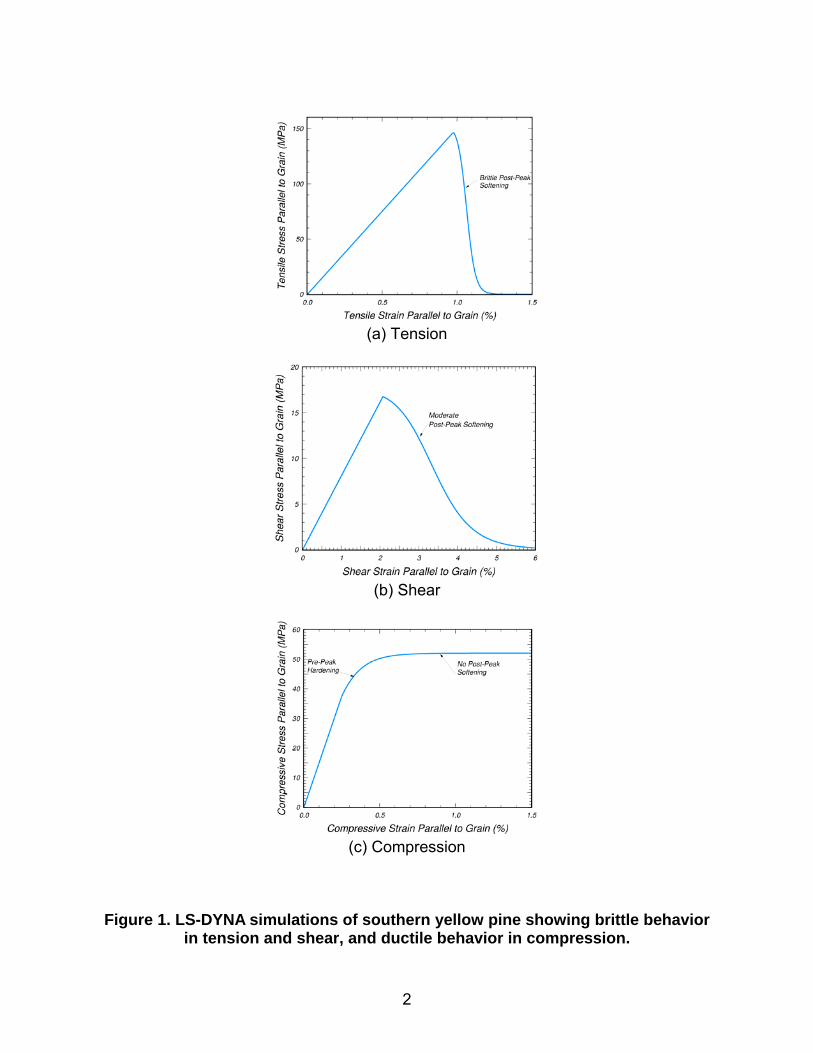
The behavior of the model is shown figure 1 for single-element LS-DYNA simulations that are conducted parallel to the grain. The simulations are linear to the peak in tension and shear, followed by post-peak softening. For these simulations, the softening is more brittle in tension than in shear. The simulation in compression is nonlinear because of the application of pre-peak hardening. No softening (perfect plasticity) is modeled in compression. A thorough discussion of the model theory is documented in the wood model manual.(2)

1.2 MODEL INPUT There are two methods of setting up the model input: The traditional method is to supply all material parameters (e.g., moduli, strengths, hardening, softening, and rate-effect parameters). A more convenient method is to request default parameters. The default parameters are obtained from laboratory data that are documented in the literature for southern yellow pine(5) and Douglas fir. The default parameters vary as a function of moisture content, temperature, and grade.

2

(a) Tension

(b) Shear

(c) Compression

Figure 1. LS-DYNA simulations of southern yellow pine showing brittle behavior in tension and shear, and ductile behavior in compression.

3

1.3 LIMITATIONS OF LABORATORY MATERIAL PROPERTY DATA One limitation of the data available for setting default parameters is that the data are for clear wood (small specimens without defects such as knots), whereas real-world posts are graded wood (e.g., grades 3, 2, and 1, or DS-65). Clear wood is stronger than graded wood. Clear wood strengths cannot be used directly as input for graded wood. Our approach for overcoming this limitation is to apply strength-reduction factors to the clear wood data, which we call quality factors, to account for reductions in strength as a function of grade. This is a practical approach compared to the alternative approach of modeling each defect explicitly. Our methodology is to estimate the quality factors from correlations with the user’s static post and Forest Products Laboratory (FPL) timber compression data. Other limitations of published laboratory test data for setting the default material properties include:

• No direct measurement of the fracture energy parallel to the grain (the fracture energy is the area under the stress-displacement curve (from peak stress to zero stress)).

• Limited information on rate effects. • Incomplete Douglas fir data. • Limited information on frozen pine properties.

Our methodology is to estimate the missing material property values through LS-DYNA correlations with static post and bogie impact data provided by the user. Thus, the LS-DYNA simulations discussed in this document not only serve to evaluate the material model, but also to set default material property values as well.

1.4 EVALUATION PROCESS The evaluation of the wood model proceeded in two steps. The first step was the evaluation of the model as a user-defined material. This means that the model was hooked up to the LS-DYNA code as material model 42 via an interface. As the developer, we retained access to the wood model source code in order to enhance the formulation and adjust the default parameters during the evaluation process. Once the evaluation was near completion and all of the default parameters were selected, the wood model was forwarded to Livermore Software Technology Corporation (LSTC) for permanent implementation into the LS-DYNA code. LSTC and the developer implemented the model into LS-DYNA, beta version 970, as material model 143. The second step was the evaluation of the wood model as material model 143 in the LS-DYNA code. The objective was to check the permanent implementation to make sure that material model 143 produced the same results as the user-defined material. Adjustments in the LSTC implementation were made until agreement was achieved.

4

All evaluation calculations documented in this report were performed by the developer with the user-defined material model. Most were conducted using LS-DYNA, version 960, on a DEC Alpha microprocessor using UNIX®. Subsequent calculations performed by the developer using material model 143 were conducted using LS-DYNA, version 970, on a personal computer (PC) using Microsoft® Windows®. Material model 143 calculations were in agreement with those performed by the developer via the interface.

1.5 VERIFICATION AND VALIDATION Verification is a check on model implementation; it determines whether the material model has been implemented as the developer had intended (i.e., without coding errors). Stress-strain histories from single-element simulations were plotted to verify implementation of the wood material model. Validation is a check on model theory; it determines whether the material model simulates real-world behavior. Multi-element simulations were compared to four sets of test data to initiate validation of the wood material model:

• Quasi-static compression tests of timbers (conduced by FPL). • Quasi-static bending tests of timbers (conducted by FPL). • Quasi-static bending tests of posts (conducted by the user). • Dynamic bogie impact tests into posts (conducted by the user).

All of the test data discussed in this report were generated and documented by FPL and the user prior to performance of this contract. Comparisons of simulations with the user’s quasi-static and dynamic post tests are used to set the quality factors, fracture energies, rate effects, and frozen pine parameters used as default parameters in the wood model. One might suggest that only pre-test predictions can be used to validate a material model. By this, we mean that the analyst is unaware of the measured results prior to the simulation. Accurate predictions (rather than correlations) certainly build the most confidence in a model. However, all calculations performed to date, and discussed in this report, were performed with the knowledge of the test results. This is because correlations with test results were used to set various default parameters. Future calculations performed by roadside safety analysts (such as the Centers of Excellence (COE) and the National Highway Traffic Safety Administration (NHTSA) National Crash Analysis Center (NCAC)) will assess the predictive capability and provide a more thorough evaluation and validation of the wood material model.

5

2 SINGLE-ELEMENT SIMULATIONS Single-element simulations were performed to help verify implementation of the wood model. Two sets of simulations are shown in figures 2 and 3 that use default material properties for southern yellow pine at room temperature. The first set is for tension parallel to the grain. The second set is for compression perpendicular to the grain. Note that both stiffness and strength vary as a function of moisture content. These simulations indicate that saturated pine properties provide the lowest stiffness and strength in both tension and compression. The posts tested statically and dynamically by the user and analyzed by the developer are all saturated (23-percent moisture content). The test posts were pulled from the field throughout Nebraska, so saturation is a reasonable test and analysis condition.

Figure 2. Good correlation between LS-DYNA simulations (dashed lines) and measured clear wood data (solid lines) for southern yellow pine in tension

parallel to the grain.

6

Figure 3. Good correlation between LS-DYNA simulations (dashed lines) and measured clear wood data (solid lines) for southern yellow pine in compression

perpendicular to the grain.

7

3 TIMBER COMPRESSION TEST CORRELATIONS FPL performed full-scale tests on dry southern yellow pine timbers in compression parallel to the grain.(6) A schematic of the test setup is reproduced in figure 4. The timber cross section is 15.24 centimeters (cm) by 15.24 cm, and the timber length is 304.8 cm. Load-deflection histories were measured for select structural and grade 2 timbers. Moisture content, failure location, and defect-initiated failures were documented. The average moisture content is 12 percent, although measurements as low as 7 percent and as high as 18 percent were recorded. The average strength measurements are:

• 25.7 MPa for select structural. • 22.7 MPa for grade 2.

The default strength of clear wood at 12-percent moisture content is 52.7 MPa.

1 inch = 25.4 millimeters (mm), 1 pound force (lbf) = 0.004448 kilonewton (kN)

Figure 4. Schematic of FPL timber compression test setup. The developer performed multi-element simulations of these tests to:

• Evaluate the behavior of the model. • Select default quality factors. • Select default hardening parameters in parallel-to-the-grain compression.

Comparisons of the simulations with the test data are shown in figure 5 as a function of grade. The black lines are the simulations. The red and colored lines are the test data. The colored lines highlight specific data curves whose strength is approximately average.

8

Load-deflection curves from two calculations are shown in each plot. One curve is a clear wood simulation that models a higher yield strength than measured. The second curve applies a strength-reduction quality factor (QC) to the compressive strength to correlate the calculated yield strength with the measured yield strength. A good correlation of the select structural simulation is obtained with a factor of QC = 0.49 applied to the compressive strength. This factor is the ratio of the average select structural timber compression strength (25.7 MPa) divided by the average clear wood compression strength (52.7 MPa) at 12-percent moisture content. A good correlation of the grade 2 simulation is obtained with a factor of QC = 0.43 applied to the compressive strength. This factor is the ratio of the average grade 2 timber compression strength (22.7 MPa) divided by the average clear wood compression strength (52.7 MPa) at 12-percent moisture content. No quality factors are applied to the stiffness, although a factor of 0.8 is probably reasonable for grade 2.

(a) Select structural (b) Grade 2

Figure 5. These comparisons of the model with test data were used to set the hardening behavior of the southern yellow pine model in parallel-to-the-grain

compression. These comparisons were made with different hardening parameter values for each grade. Good correlations could not be achieved using the same hardening parameter values for each grade. Therefore, the default material property methodology was set up to specify hardening parameters as a function of grade. This is more thoroughly discussed in the wood model user’s manual.(2)

9

4 TIMBER-BENDING TEST CORRELATIONS FPL performed full-scale tests of southern yellow pine timbers in parallel-to-the-grain four-point bending.(6) The timber cross section is 15.24 cm by 25.24 cm, and the timber length is 304.8 cm. Load-deflection histories were measured for select structural and grade 2 timbers. Moisture content and failure mode were recorded. The average moisture content is 14 percent, although measurements as low as 9 percent and as high as 23 percent were recorded. The developer performed multi-element simulations of one or more tests to evaluate the bending response of the wood material model and to select quality factors in tension. Comparisons of the simulations with measured load-deflection curves are shown in figure 6 as a function of grade. The black lines are the simulations. The red and colored lines are the test data. The colored lines highlight specific data curves for better viewing. Load-deflection curves from three calculations are shown in each plot. One curve is a clear wood simulation that models a higher bending strength than that measured. The second curve applies a quality factor to the tensile strength (QT) that is equal to the quality factor applied to the compressive strength (QC). The QC value is that selected from the timber compressive simulations discussed in the previous section. These simulations also model higher bending strengths than those measured. The third curve applies a tensile quality factor that is less than the compressive factor. In addition, a quality factor is also applied to the stiffness (Qstiff). These simulations correlate well with the measured data. A good correlation of the select structural simulation is obtained with a quality factor of QT = 0.25. This value is much lower than that previously selected in compression (QC = 0.49). A good correlation of the grade 2 simulation is obtained with a quality factor of QT ≤ 0.25. This value is also lower than that previously selected in compression (QC = 0.43). These correlations prompted the developer to model different quality factors in tension than in compression. The tensile quality factors are also applied to the shear strength. Also note that a quality factor of 0.8 is applied to the stiffness for correlation with the test data (for both grades), although a quality factor of 1.0 is still reasonable. No methodology is currently implemented in the initialization routines of material model 143 to specify quality factors for stiffness. This is because clear wood stiffnesses are adequate for simulating graded wood stiffnesses based on calculations performed to date. However, quality factors for stiffness could readily be added if the need arises.

10

(a) Select structural

(b) Grade 2

Figure 6. These comparisons of the model with the parallel-to-the-grain timber-bending test data demonstrate the need for different quality factors in tension

and compression.

11

5 QUASI-STATIC POST TEST CORRELATIONS The main reason for developing the wood material model is to analyze wood posts in roadside safety applications. Such posts are often saturated. Although the FPL data discussed in the preceding sections are useful for model evaluation and input parameter selection, the data focus on dry timbers rather than saturated wood posts. Therefore, additional bending test correlations are reported here for saturated wood posts. The main objective for simulating the user’s quasi-static tests is to select specific default parameters, namely, quality factors and parallel-to-the-grain fracture energies, as a function of grade. The user’s test data are reviewed first, followed by correlation of the LS-DYNA simulations with the test data. Finally, the results from a number of parametric studies are reported.

5.1 SOUTHERN YELLOW PINE BENDING TEST DATA The user conducted 25 bending tests on southern yellow pine posts of three grades (DS-65, 1D, and 1).(7) The grading was performed without considering waning on the ends of the posts. The posts were removed from the field from guardrail installations throughout Nebraska. They were cantilevered in a rigid frame and were loaded at a constant rate (as shown in figure 7). In some tests, neoprene and steel were wedged between the wood post and the steel support (as shown in figure 8). Load and deformation were continuously recorded. All post failure was dominated by tensile failure of the growth rings.

Figure 7. Quasi-static post test setup.

12

(a) Steel at bottom of support (b) Neoprene at top of support on compression side Figure 8. Details for the rigid frame used in the quasi-static post test setup.

Peak force, deflection, and energy are listed in table 1. Moderate scatter is observed in the data. For the grade 1 and DS-65 posts, all peak-force measurements are within 20 percent of the average measurements. For the grade 1D posts, all peak-force measurements are within 33 percent of the average measurement. For example, for grades 1 and 1D posts, peak forces range from 24.0 to 72.5 kilonewtons (kN) and deflections at peak force range from 30.5 to 94.0 mm. For DS-65 posts, peak forces range from 53.8 to 77.8 kN and deflections at peak force range from 43.2 to 91.4 mm.

Table 1. Average of static post test data by grade.

Peak Force

Grade

Number of

Posts Force (kN)

Deflection (mm)

Energy (kN-mm)

DS-65 1D 1

10 7 8

67 55 42

68 49 53

3040 1970 1440

Deformed configurations from one grade DS-65 and one grade 1 southern yellow pine specimen are given in figure 9. Closeup views of damage in the break region are given in figure 10. Example load-deflection histories are given in figure 11. The curves exhibit slight pre-peak nonlinearity, followed by sudden drops in load as the specimens fail in the tensile region.

13

(a) DS-65 test 1420 (b) Grade 1 test 418

Figure 9. Deformed configurations of posts in static tests.

(a) DS-65 post (b) Grade 1D post

Figure 10. Closeup of damage observed in break region of posts in static tests.

14

Figure 11. Measured load-deflection histories exhibit sudden drops in force as the post fails in the tensile region.

The user developed performance envelopes from quasi-static load-deflection and energy-deflection curves. These envelopes are shown in figure 12, along with the performance envelopes developed from the dynamic bogie impact tests (to be discussed later). The user constructed the envelopes using curves from posts that exhibited the most typical behavior. For example, the DS-65 performance envelopes were developed from 6 of the 10 tests reported in table 1. The grade 1 performance envelopes were also developed from some, but not all, of the 15 tests reported in table 1. The grade 1 performance envelopes represent the combined curves from the grades 1 and 1D tests because the behavior of the grades 1 and 1D posts was similar. Note that the minimum and maximum curves that define the performance envelopes do not represent any one particular curve from the tests. Measured curves plotted by the user are reproduced in figure 13 for grades 1 and 1D. Showing all of the curves allows us to better see the character of the data (such as scatter and sudden drops in force). This is important because the static post test analyses performed by the developer, which are discussed in the next section, exhibit large variations in post-peak behavior and sudden drops in force. A comparison of the performance envelopes in figure 12 with the measured data curves in figure 13 suggests that the static performance envelopes are developed from data that exhibit the largest fracture energies. The relatively small scatter of the performance envelopes is surprising, especially considering that the failure (softening) curves are being measured. For example, see the scatter in the data measured by FPL for their timber compression and bending tests in figures 5 and 6. The reader is also referred to appendixes A and B of the wood model user’s manual(2) for plots of clear wood stiffness and strength measurements. Clear wood stiffnesses (and strengths) vary by a factor of three from high measurement to low measurement.

15

Figure 12. Quasi-static (blue solid line) and dynamic (pink dashed line) performance envelopes developed and plotted by the user.

(a) Force versus deflection

(b) Energy versus deflection

16

(a) Force versus deflection

(b) Energy versus deflection

Figure 13. Grades 1 and 1D static post test measurements exhibit substantial scatter.

5.2 LS-DYNA CORRELATIONS Multi-element simulations of guardrail posts in bending were performed at two grade levels for comparison with the performance envelopes (as shown in figures 14 and 15). Good correlations in the loading region primarily determine the tensile and compressive quality factors. The compressive quality factor also has a significant effect on the late-time softening response. The quality factors selected were QT = 0.47 with QC = 0.63 for grade 1 posts, and QT = 0.80 with QC = 0.93 for DS-65 posts.

90

45

0

Forc

e (k

N)

90

45

0

Forc

e (k

N)

(mm) 0 51 102 152 203 254

(mm) 0 51 102 152 203 254

(mm) 0 51 102 152 203 254

(mm) 0 51 102 152 203 254

11.3 5.6

0

Ene

rgy

(kN

-mm

) (E

+03)

11.3 5.6

0

Ene

rgy

(kN

-mm

) (E

+03)

17

Good correlations in the post-peak softening region determine the parallel-to-the-grain fracture energies. Parallel fracture energies (Gf ||) are reported here as multiples of the perpendicular fracture energies (Gf ⊥). Fracture energies used in these simulations are Gf || = 250 Gf ⊥ kN-mm for grade 1 and Gf || = 380 Gf ⊥ kN-mm for DS-65, with B = 30 for both grades. Deformed configurations at 200 milliseconds (ms) (approximately 190 mm) are shown in figure 16, along with fringes of damage. The damage plotted is the maximum of the parallel and perpendicular damage. High damage (greater than 80 percent) is indicated by the red elements.

18

(a) Force versus deflection

(b) Energy versus deflection

Figure 14. Good correlations between the LS-DYNA calculations and quasi-static performance envelopes determine the default quality factors for grade 1 southern

yellow pine of QT = 0.47 with QC = 0.63.

19

(a) Force versus deflection

(b) Energy versus deflection

Figure 15. Good correlations between the LS-DYNA calculations and quasi-static performance envelopes determine the default quality factors for DS-65 southern

yellow pine of QT = 0.80 with QC = 0.93.

20

(a) Grade 1 deformed configuration (b) Fringes of damage

(c) DS-65 deformed configuration (d) Fringes of damage

Figure 16. The parallel-to-the-grain post fracture calculated in the post just below

the top of the rigid support is in agreement with the location of the damage observed in the tests.

21

Details for the geometric models and parametric calculations used to establish these default parameters are given in the following section.

5.3 LS-DYNA PARAMETRIC STUDIES Various parametric calculations were conducted to further evaluate the material model and default material property selection. Meshing: The parametric calculations were performed with three geometric models as shown in figure 17. The first geometric model uses fixed nodal constraints, without the use of slide surfaces. Neither the steel support nor the loading bolt is modeled. Therefore, it is the fastest running model. The second geometric model uses planar rigid walls of a finite size to model the steel support. The slide surface between the wood post and the rigid wall is modeled with a coefficient of friction of 0.30. In addition, the steel loading bolt is explicitly modeled. The third geometric model explicitly meshes the steel support as brick elements of rigid material. This mesh was developed by the user.

(a) Fixed nodes (b) Rigid walls (c) Full-support structure

Figure 17. Three geometric models were set up for performing parametric calculations.

Load-deflection curve comparisons are given in figure 18 for the full-support and rigid-wall models. Behaviors are similar, as though the load-deflection curve of the full-support model is shifted relative to the rigid-wall model. All default quality factors were selected from final calculations performed with the full-support structure. However, most parametric calculations were performed with either the rigid-wall model or the fixed-

Applied Velocity

X

No X or Z displacement

No X or Zdisplacement

Z

22

node model. This is because the rigid-wall model runs 15 times faster than the full-support model, while the fixed-node model runs 45 times faster than the full-support structure. Unless otherwise stated, all parametric calculations reported in this section are conducted with the rigid-wall model.

(a) Force deflection (b) Energy deflection

Figure 18. The force-deflection curve calculated with the fast-running, rigid-wall model is similar to that calculated with the full-support structure, making it useful

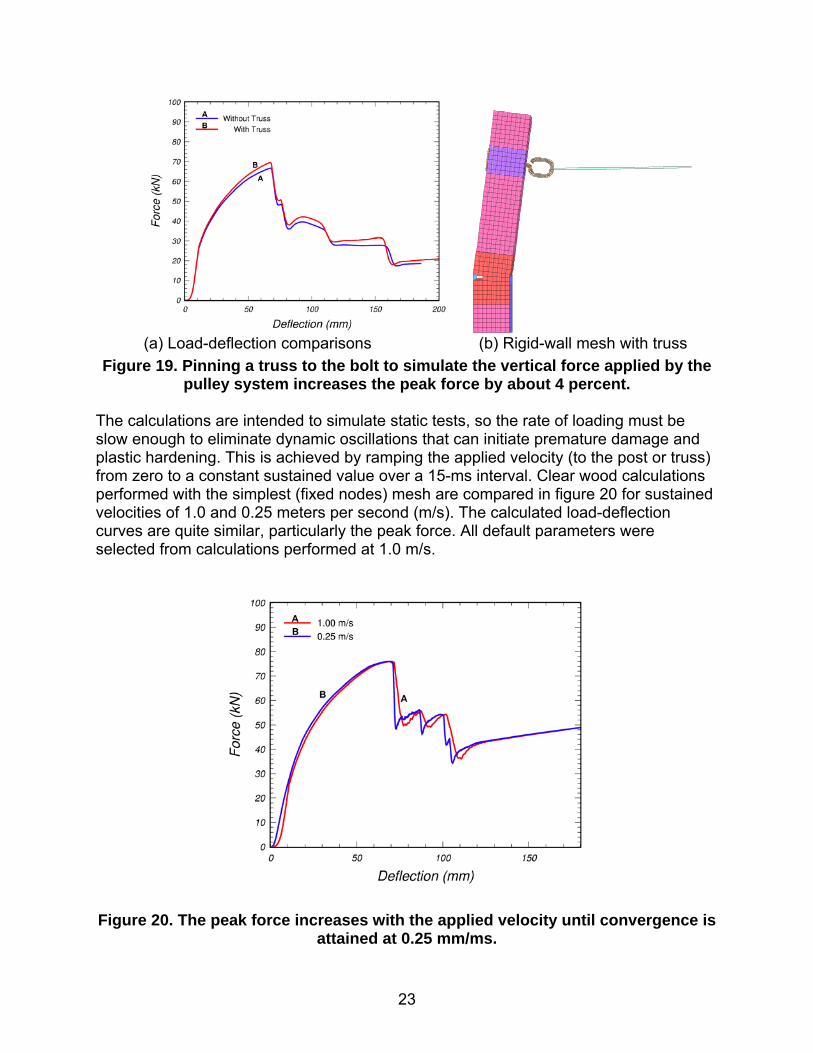
for performing parametric calculations. Loading Method and Rate: The method of loading the bolt has a minor effect on the calculated response. This is demonstrated in figure 19(a) for two loading methods. In the first method, horizontal velocity is applied to the rigid bolt (or post). This means that no vertical forces are applied to the bolt, so the post is free to rotate. In the second method, horizontal velocity is applied to the end of a truss that is pinned to the bolt (as shown in figure 19(b)). This means that small vertical forces are applied to the bolt to simulate the effect of the pulley system on post rotation. The pulley system of the test configuration was previously shown in figure 7. It was used to load the bolt attached to the wood post. Application of the pinned truss increases the peak force by about 4 percent. All default parameters were selected from calculations performed with the truss. The calculations previously shown in figure 18 were performed with a truss.

23

(a) Load-deflection comparisons (b) Rigid-wall mesh with truss

Figure 19. Pinning a truss to the bolt to simulate the vertical force applied by the pulley system increases the peak force by about 4 percent.

The calculations are intended to simulate static tests, so the rate of loading must be slow enough to eliminate dynamic oscillations that can initiate premature damage and plastic hardening. This is achieved by ramping the applied velocity (to the post or truss) from zero to a constant sustained value over a 15-ms interval. Clear wood calculations performed with the simplest (fixed nodes) mesh are compared in figure 20 for sustained velocities of 1.0 and 0.25 meters per second (m/s). The calculated load-deflection curves are quite similar, particularly the peak force. All default parameters were selected from calculations performed at 1.0 m/s.

Figure 20. The peak force increases with the applied velocity until convergence is

attained at 0.25 mm/ms.

24

Filtering: All static computational force histories are also post-processed using the Society of Automotive Engineers (SAE International) 60 filter in LS-TAURUS (an LS-DYNA post-processor) to remove the high-frequency post-peak oscillations that occur as the elements soften in the tensile region. A different filtering method is used for the bogie impact calculations discussed later. Filtering is used because it is not practical to run the calculations slow enough to eliminate all post-peak oscillations; the calculations are quasi-static rather than static. The filtering primarily clarifies the post-peak softening response for comparison with the unfiltered test data. One comparison between clear wood calculations, with and without filtering, is shown in figure 21. These calculations were performed with the simplest (fixed nodes) mesh.

Figure 21. Quasi-static calculations are filtered for easier comparison with the

unfiltered test data. Fracture Energy: The calculated response depends on the value of the parallel-to-the-grain fracture energy. Comparisons at two different fracture energy levels are shown in figure 22. The greater the parallel fracture energy, the more gradual the post-peak softening response, and the more energy it takes to break the post. These comparisons were performed with B = 30, and QT = 0.47 with QC = 0.63. The two values used in the simulations are Gf || = 250 Gf ⊥ kN-mm and Gf || = 50 Gf ⊥ kN-mm for grade 1. Here, Gf || is the parallel-to-the-grain fracture energy and Gf ⊥ is the perpendicular-to-the-grain fracture energy. The 250 value is obtained from correlations with the static performance envelopes. The 50 value is obtained from correlations with the dynamic performance envelopes (discussed in subsequent sections). Although the peak forces are similar, the post-peak response is substantially different. The calculation conducted with Gf || = 50 Gf ⊥ kN-mm does not fit within the performance envelopes; however, it does correlate well with the suite of measured data previously plotted in figure 13. In this figure, 9 out of 15 of the data curves peak between 25 and 50 mm of deflection and then exhibit a sudden drop in force. The calculation is consistent with the measured behavior.

25

Figure 22. The energy required to break the post increases as the value of the

parallel-to-the-grain fracture energy increases. Compressive Quality Factor: For a given fracture energy, the softening response also depends on the compressive quality factor. Two computational comparisons are shown in figure 23. The calculation with QT = QC = 0.60 gives approximately the same peak force as the calculation with QT = 0.47 with QC = 0.63, but does not soften as rapidly. Numerous parametric calculations have demonstrated that increasing the value of QC above QT increases the force at the peak, but decreases the force at a large deflection (reduces the tail). This is because yielding in the compressive region is delayed by increasing QC. Allowing QC to be greater than QT is consistent with our fits to the FPL static bending test data previously shown in figure 6. All default quality factors were selected with QC greater than QT.

(a) Force deflection (b) Energy deflection Figure 23. Calculations with QC > QT soften more rapidly than calculations with QC

= QT.

26

Softening Shape Parameter: The calculated response also depends on the value of the softening parameter B (as shown in figure 24). The greater the value of B, the greater the peak force. Recall that the parameter B determines the shape of the softening curve in single-element simulations. This is shown in figure 25 for tension parallel to the grain. A moderate value of B = 30 was selected for use as a default parameter. This value is somewhat arbitrary because no softening-curve measurements are available from the FPL direct-pull simulations for fitting the softening model. Softening curves are often difficult to measure. These clear wood calculations were performed with the simplest mesh at 1 m/s using Gf || = 300 Gf ⊥.

Figure 24. The calculated peak force increases with increasing values of the

softening parameter B.

Figure 25. The softening parameter B determines the shape of the softening curve

in these single-element simulations for tension parallel to the grain.

27

Hourglass Control: The calculated response also depends on the hourglass control. To demonstrate this, calculations performed with viscous and stiffness hourglass controls are compared to a calculation performed with selectively reduced (S/R) integrated elements (ELFORM 2 is called a fully integrated S/R solid). Deformed configurations in the break region are shown in figure 26. Load-deflection curves are shown in figure 27. Hourglass energy histories are shown in figure 28. The simulation with viscous hourglass control exhibits hourglassing at an early time, resulting in an unrealistic pinching behavior on the backside of the post in the compressive region near ground level. Hourglassing is concentrated in the breakaway region of the post, where the damage accumulates. Type 3 viscous control, with a default coefficient of QM = 0.1, was used throughout the post breakaway region. The simulation with stiffness hourglass control exhibits less visual hourglassing and pinching. Type 4 stiffness control, with a reduced coefficient of QM = 0.005, was used throughout the post breakaway region. The third simulation was performed with fully integrated elements (eight integration points) in the breakaway region. Fully integrated elements do not require hourglass control. Note that the deformed configuration and the peak force calculated with stiffness hourglass control are in best agreement with those calculated with the fully integrated elements. One common concern is that stiffness hourglass control overstiffens the calculated response. These comparisons indicated that stiffness hourglass control does not stiffen the calculated response unrealistically. In fact, the calculation with stiffness control matches the peak force calculated with fully integrated elements. In addition, the final hourglass/internal energy ratio in the breakaway region is slightly less with stiffness control than with viscous control. Therefore, stiffness hourglass control with QM = 0.005 was used in the breakaway region of all calculations involving default parameter selection. As a bonus, the calculation with stiffness control runs the fastest. The viscous control and fully integrated element calculations run 7 percent and 51 percent longer, respectively, than the stiffness control calculation.

28

(a) Viscous control (b) Stiffness control (c) Fully integrated S/R

120-mm deflection

(d) Viscous control (e) Stiffness control (f) Fully integrated S/R

190-mm deflection

Figure 26. Type 4 stiffness control reduces hourglassing better than type 3 viscous control.

29

Figure 27. The peak force calculated with type 4 stiffness control agrees with the

fully integrated element calculation better than the type 3 viscous calculation.

Figure 28. Less final hourglass energy is calculated with type 4 stiffness control

than with type 3 viscous control. Moisture Content: Moisture content has a strong effect on the calculated load-deflection curves (as shown in figure 29). The peak force calculated in the post at 17- percent moisture content is 80 percent greater than the peak force calculated in the post at 23-percent (saturated) moisture content. Calculations with variations in moisture content along the length of the post were also performed. One calculation was performed with three regions of differing moisture content, while a second calculation was performed with five regions of differing moisture content. The moisture content at ground level, where parallel-to-the-grain fracture

30

occurs, has the greatest effect on the force in the post. These calculations were performed with the simplest (fixed nodes) mesh.

Figure 29. Decreasing the moisture content by 6 percent increases the post-peak

force by 80 percent.

(a) 3 MC levels

18.5% 18.5%

20.0%

23.0% 23.0%

21.0% 20.0%

22.0%

(b) 5 MC levels (c) Force versus deflection

31

6 DYNAMIC POST TEST CORRELATIONS The main objectives of the dynamic post test correlations are to evaluate the wood material model and to select specific default parameters. Although we mainly expected to select rate-effect parameters as a function of grade, we instead adjusted the parallel fracture energies previously selected from the static post tests. The user’s bogie impact test data are reviewed first, followed by correlation of the LS-DYNA simulations with the test data. Then, filtering and sampling issues are discussed. Finally, the results from a number of parametric studies are reported. Wood posts installed in the field are typically situated in a deformable medium (such as soil or concrete). The post/medium interaction complicates validation of the wood model. Here, wood posts installed in a fixed-type base are analyzed to eliminate post/medium interaction and to facilitate evaluation of the wood model.

6.1 BOGIE IMPACT TEST DATA The user conducted 80 bogie tests on southern yellow pine posts of five grades (DS-65, 1D, 1, 2D, and 2) and 7 tests on Douglas fir posts of one grade (1).(6) Significant knots and defects were cataloged. The posts were placed in a steel tube embedded in reinforced concrete (as shown in figure 30). The post/steel interface was padded with neoprene on the front and back. The posts were impacted at approximately 9.6 m/s by a 944-kilogram (kg) bogie. A summary of the test results at peak force and rupture is given in table 2. Example force, velocity, and deflection histories are given in figure 31. An accelerometer was located near the center of the bogie frame. Force, velocity, and deflection were derived from the measured deceleration. Post damage in the breakaway region of the post, just below ground level, is shown in figure 32.

32

Figure 30. Post setup for dynamic bogie impact tests.

Table 2. Summary of bogie impact tests on posts by grade.

Peak Force Rupture Number of

Posts

Grade Force

(kN) Time(ms)

Defl. (mm)

Energy (kN-mm)

Time (ms)

Defl. (mm)

Energy (kN-mm)

16 16 9 7 16 16 7 5 7

DS-65 1D 1 (Worst) 1 (Random) 2D 2 Douglas Fir Frozen DS-65 Frozen 1

95 49 38 47 52 44 46 62 43

9.0 8.2 9.3 8.3 8.6 9.1 8.4 7.9 7.9

86.3 78.7 86.3 81.2 83.8 88.9 81.2 76.2 76.2

4462.6 2265.4 1867.0 2151.6 2424.8 2151.6 2151.6 2686.6 1878.4

18.8 15.4 18.0 15.5 17.5 16.7 15.9 14.5 14.9

170.1 144.7 162.5 149.8 165.1 160.0 149.8 139.7 142.2

8811.4 4212.1 3608.8 4132.4 4758.6 4041.4 4075.5 5122.9 3563.2

Impact

33

(a) Force deflection

(b) Velocity time

(c) Displacement time

Figure 31. Processed data from the user’s bogie impact tests.

34

(a) DS-65 pine (b) Grade 1 pine

(c) Grade 1 frozen pine (d) Grade 1 fir

Figure 32. Damage in the breakaway region of the posts, just below ground level. These test results provide information on post performance versus grade. The user’s results indicate that the DS-65 posts are significantly stronger than all other posts. In addition, the user reports that there is no statistically significant difference in the energy absorbed by the dense and low-density posts. Thus, the posts can be effectively divided into two grades―high (DS-65) and low (all others). These test results also provide information on rate effects. The peak force measured in the dynamic bogie tests is 1.42 times that measured in the static bending tests for the DS-65 posts. Dynamic and static peak forces are similar for the grade 1 posts. This is seen by examining the static and dynamic performance envelopes previously shown in figure 12.

6.2 LS-DYNA CORRELATIONS The developer performed LS-DYNA simulations of the bogie impact tests for four combinations of post material and grade. These combinations are grade 1 southern yellow pine, DS-65 southern yellow pine, grade 1 frozen pine, and grade 1 Douglas fir. Calculated energy-deflection curves are compared to the user’s performance envelopes and measured curves in figures 33 through 36. Calculated bogie velocity-reduction histories are also compared to the user’s measured histories.

35

(a) Energy (b) Velocity reduction

Figure 33. These correlations between the LS-DYNA calculations and the performance envelopes were used to adjust the parallel fracture energy for

grade 1 pine to 50 times the perpendicular fracture energy.

(a) Energy (b) Velocity reduction

Figure 34. These correlations between the LS-DYNA calculations and the performance envelopes were used to adjust the parallel fracture energy for DS-65

pine to 85 times the perpendicular fracture energy.

36

(a) Energy versus deflection (b) Velocity versus time Figure 35. These correlations between the LS-DYNA calculations and the energy-

deflection data were used to confirm that grade 1 Douglas fir can be simulated with the same parallel fracture energy and rate-effect parameters as grade 1

southern yellow pine, but with different quality factors.

(a) Force versus deflection (b) Velocity versus time

Figure 36. These correlations between the LS-DYNA calculations and the energy-

deflection data were used to set the parallel fracture energy for frozen grade 1 pine to five times the perpendicular fracture energy.

The first comparison in figure 33 is for grade 1 pine. Although a parallel fracture energy of 250 Gf ⊥ was selected from static post correlations, a parallel fracture energy of 50 Gf ⊥ provides a better correlation with the dynamic performance envelopes. The reason for the discrepancy in the fracture energy is not known; however, there are two possibilities:

37

• The static performance envelopes are biased toward high fracture energy, as previously discussed.

• The boundary conditions in both the static and dynamic tests are not well defined and are difficult to model computationally. The selection of fracture energy, particularly for the static simulations, is dependent on how the boundary conditions are modeled.

The expected application of the wood model is dynamic, so all default parallel fracture energies are those that are identified through dynamic correlations. On the other hand, all quality factors used in the dynamic calculations are identical to those used in the static calculations; thus, there is no ambiguity about the default quality factors. Similarly, for the DS-65 pine simulations in figure 34, the statically selected fracture energy of Gf || = 380 Gf ⊥ is adjusted downward to Gf || = 85 Gf ⊥ in order to obtain good correlation with the measured data. For grade 1 Douglas fir simulations in figure 35, the correlations are obtained using the same fracture energy as for grade 1 pine, but with slight adjustments in the pine quality factors. For frozen grade 1 pine simulations in figure 36, the correlations are obtained with the same quality factors as for unfrozen grade 1 pine, but with a drastic reduction in the fracture energy from Gf || = 50 Gf ⊥ to Gf || = 5 Gf ⊥ to make the frozen pine more brittle than the unfrozen pine. Deformed configurations for the grade 1 pine simulations are shown in figure 37. Figure 37(a) shows the post surrounded by the rigid support structure. The wood post mesh with the rigid support structure was created by the user. This support structure is removed in figure 37(b) to better view the post failure location. The post breaks just below ground level, in agreement with the location of the breakage observed in the tests. Neoprene, modeled as an elastic material with external damping, is visible along the front and back faces of the post.

38

(a) With rigid support (b) Without rigid support (c) Fringes of damage

Figure 37. The simulated post breaks just below ground level, in agreement with

the failure location observed in the tests. Figure 37(c) shows fringes of damage in the post, as indicated by the colored elements. The highest levels of damage (above 80 percent) are indicated by the red elements. These fringes indicate a large split in the post running downward below ground level, consistent with the type of damage observed in the tests. Slight damage is also visible in the impact region, although impact damage was not reported in the tests.

6.3 FILTERING AND SAMPLING ISSUES It is important to note that good correlation between the calculated and measured data not only depends on the wood post model, but on the bogie model (geometric and material models) as well. This is because the performance envelopes were derived from deceleration measurements recorded by an accelerometer placed near the center of the bogie frame. No measurements were made on the wood post or the bogie cylinder. The deceleration measurements were sampled at 3200 hertz (Hz) and filtered according to SAE J-211 specifications using a channel frequency class (CFC) filter of 60 Hz (CFC 60). The filtered deceleration histories were multiplied by the bogie mass (approximately 944 kg) to convert to force histories. The filtered deceleration histories were also integrated to form bogie velocity-reduction and post deflection histories. A more thorough discussion of the user’s data-processing technique is given in reference 9.

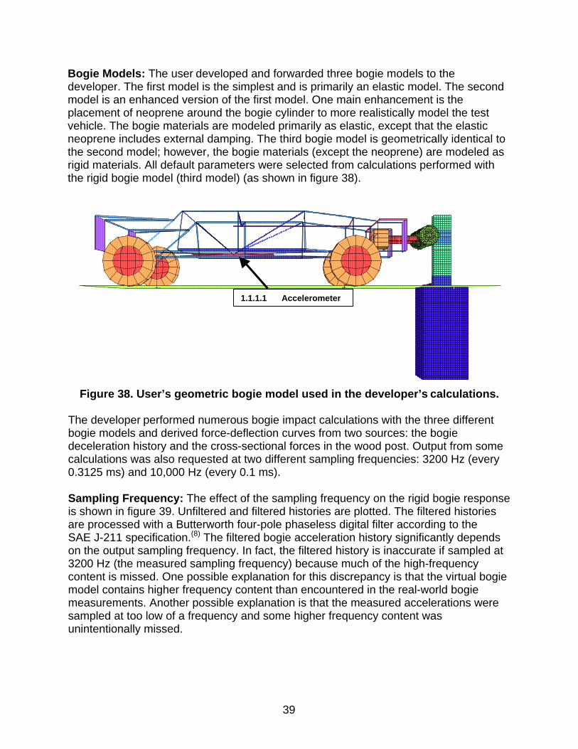
39

Bogie Models: The user developed and forwarded three bogie models to the developer. The first model is the simplest and is primarily an elastic model. The second model is an enhanced version of the first model. One main enhancement is the placement of neoprene around the bogie cylinder to more realistically model the test vehicle. The bogie materials are modeled primarily as elastic, except that the elastic neoprene includes external damping. The third bogie model is geometrically identical to the second model; however, the bogie materials (except the neoprene) are modeled as rigid materials. All default parameters were selected from calculations performed with the rigid bogie model (third model) (as shown in figure 38).

C

Figure 38. User’s geometric bogie model used in the developer’s calculations.

The developer performed numerous bogie impact calculations with the three different bogie models and derived force-deflection curves from two sources: the bogie deceleration history and the cross-sectional forces in the wood post. Output from some calculations was also requested at two different sampling frequencies: 3200 Hz (every 0.3125 ms) and 10,000 Hz (every 0.1 ms). Sampling Frequency: The effect of the sampling frequency on the rigid bogie response is shown in figure 39. Unfiltered and filtered histories are plotted. The filtered histories are processed with a Butterworth four-pole phaseless digital filter according to the SAE J-211 specification.(8) The filtered bogie acceleration history significantly depends on the output sampling frequency. In fact, the filtered history is inaccurate if sampled at 3200 Hz (the measured sampling frequency) because much of the high-frequency content is missed. One possible explanation for this discrepancy is that the virtual bogie model contains higher frequency content than encountered in the real-world bogie measurements. Another possible explanation is that the measured accelerations were sampled at too low of a frequency and some higher frequency content was unintentionally missed.

1.1.1.1 Accelerometer

40

(a) Calculated acceleration histories (b) Calculated force-deflection histories

Figure 39. The filtered bogie acceleration history sampled at 3200 Hz is significantly different than the history sampled at 10,000 Hz.

Filtered force-deflection curves derived from the calculated deceleration history are compared to the processed test data in figure 39(b). The comparisons demonstrate that the peak force of the calculation sampled at 3200 Hz is overpredicted. The peak force of the calculation sampled at 10,000 Hz is roughly the same as that of the measured data. These calculations are preliminary (prior to selection of the final default parameters previously shown in figure 33) and were performed with QT = QC = 0.6 and Gf || = 50 Gf ⊥ with no rate effects. Model Type: The bogie model type (rigid or elastic) also affects the calculated acceleration histories. Calculated force-deflection curves from the elastic (first model) and rigid bogies are compared to each other in figure 40 and to a grade 1 pine measurement. Two curves are plotted for the elastic bogie. One curve is derived from a nodal acceleration calculated on the bogie frame at the approximate gauge location of the real-world bogie. It exhibits substantial oscillations despite being filtered and does not correlate well with the measured data. The other curve is derived from a nodal acceleration calculated on the bogie cylinder. It is less oscillatory, with a peak force similar to that of the measured data, although the curve shape is qualitatively different from that of the measured data.

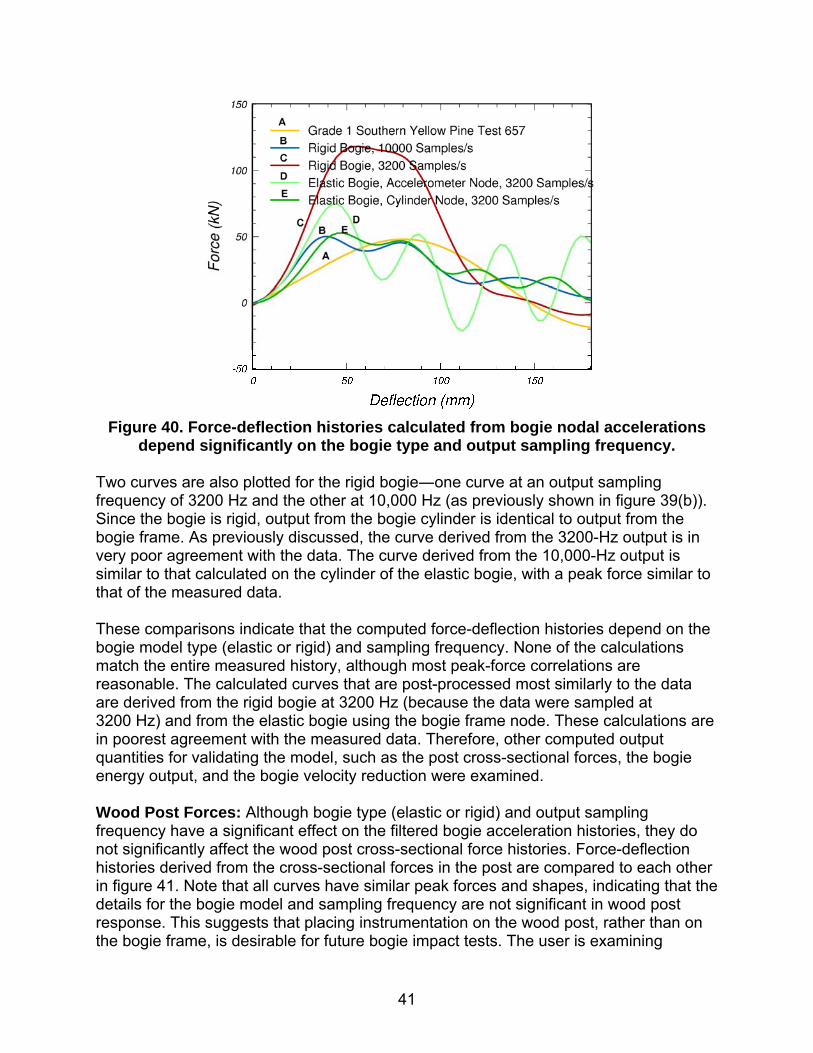
41

Figure 40. Force-deflection histories calculated from bogie nodal accelerations

depend significantly on the bogie type and output sampling frequency. Two curves are also plotted for the rigid bogie―one curve at an output sampling frequency of 3200 Hz and the other at 10,000 Hz (as previously shown in figure 39(b)). Since the bogie is rigid, output from the bogie cylinder is identical to output from the bogie frame. As previously discussed, the curve derived from the 3200-Hz output is in very poor agreement with the data. The curve derived from the 10,000-Hz output is similar to that calculated on the cylinder of the elastic bogie, with a peak force similar to that of the measured data. These comparisons indicate that the computed force-deflection histories depend on the bogie model type (elastic or rigid) and sampling frequency. None of the calculations match the entire measured history, although most peak-force correlations are reasonable. The calculated curves that are post-processed most similarly to the data are derived from the rigid bogie at 3200 Hz (because the data were sampled at 3200 Hz) and from the elastic bogie using the bogie frame node. These calculations are in poorest agreement with the measured data. Therefore, other computed output quantities for validating the model, such as the post cross-sectional forces, the bogie energy output, and the bogie velocity reduction were examined. Wood Post Forces: Although bogie type (elastic or rigid) and output sampling frequency have a significant effect on the filtered bogie acceleration histories, they do not significantly affect the wood post cross-sectional force histories. Force-deflection histories derived from the cross-sectional forces in the post are compared to each other in figure 41. Note that all curves have similar peak forces and shapes, indicating that the details for the bogie model and sampling frequency are not significant in wood post response. This suggests that placing instrumentation on the wood post, rather than on the bogie frame, is desirable for future bogie impact tests. The user is examining

42

methods of placing instrumentation on the posts; however, post breakage and splitting complicate the task.

Figure 41. Force-deflection histories calculated from the wood post cross-

sectional forces are not significantly affected by the details for the bogie model or sampling frequency.

The wood post force-deflection curves are also compared to the one measured bogie curve in figure 41. Note that the calculated and measured peak forces are similar; however, the calculated response softens faster than the measured response. This indicates that less energy is being calculated in the wood post than is measured from the bogie (as shown in figure 42). The energy-deflection curves are derived by integrating the force-deflection curves. The reduction in bogie kinetic energy (as measured by the accelerometer) is primarily balanced by the energy needed to break the post (as calculated via the cross-sectional forces), plus the kinetic energy of the broken post, and the energy lost to post sliding and neoprene damping. Therefore, it is expected that the post energy calculated from the cross-sectional forces would be less than the bogie kinetic energy reduction. This means that direct correlations between the calculated post energy and the measured bogie energy cannot be made. These calculations were preliminary and were performed with QT = QC = 0.6 and Gf || = 50 Gf ⊥ with no rate effects.

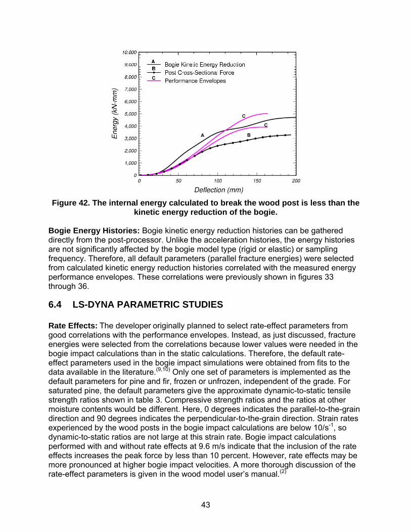
43

Figure 42. The internal energy calculated to break the wood post is less than the

kinetic energy reduction of the bogie. Bogie Energy Histories: Bogie kinetic energy reduction histories can be gathered directly from the post-processor. Unlike the acceleration histories, the energy histories are not significantly affected by the bogie model type (rigid or elastic) or sampling frequency. Therefore, all default parameters (parallel fracture energies) were selected from calculated kinetic energy reduction histories correlated with the measured energy performance envelopes. These correlations were previously shown in figures 33 through 36.

6.4 LS-DYNA PARAMETRIC STUDIES Rate Effects: The developer originally planned to select rate-effect parameters from good correlations with the performance envelopes. Instead, as just discussed, fracture energies were selected from the correlations because lower values were needed in the bogie impact calculations than in the static calculations. Therefore, the default rate-effect parameters used in the bogie impact simulations were obtained from fits to the data available in the literature.(9,10) Only one set of parameters is implemented as the default parameters for pine and fir, frozen or unfrozen, independent of the grade. For saturated pine, the default parameters give the approximate dynamic-to-static tensile strength ratios shown in table 3. Compressive strength ratios and the ratios at other moisture contents would be different. Here, 0 degrees indicates the parallel-to-the-grain direction and 90 degrees indicates the perpendicular-to-the-grain direction. Strain rates experienced by the wood posts in the bogie impact calculations are below 10/s-1, so dynamic-to-static ratios are not large at this strain rate. Bogie impact calculations performed with and without rate effects at 9.6 m/s indicate that the inclusion of the rate effects increases the peak force by less than 10 percent. However, rate effects may be more pronounced at higher bogie impact velocities. A more thorough discussion of the rate-effect parameters is given in the wood model user’s manual.(2)

44

Table 3. Approximate tensile strength ratios versus strain rate for saturated pine.

Rate (s-1) ℜ(0°) ℜ(90°) 0

10 500

1000

1.0 1.01 1.3 1.6

1.0 1.2 7.2 12.6

Post Breakage: The bogie impact test report does not indicate the time or deflection at which the post broke completely in two. The simulated deformed configurations previously shown in figure 37 indicate that the breakage is incomplete at 180 mm, which is the final deflection of the performance envelope plots. Although this may or may not be correct, parametric studies were performed and it was determined that adjustments in the quality factors affect the deflection at which the post breaks in two. This is demonstrated in figure 43. Here, the default quality factors were adjusted for grade 1 pine from QT = 0.47 and QC = 0.63 to QT = 0.4 and QC = 0.7. The trend noted is that the post will break earlier in time as QT is adjusted downward and QC is adjusted upward. The load-deflection and bogie velocity-reduction curves calculated with either set of quality factors look similar (as shown in figure 44).

45

C

(a) QT = 0.47 and QC = 0.63 (b) QT = 0.40 and QC = 0.70

Figure 43. These deformed configurations at 180 mm of deflection indicate that adjustments in the quality factors affect the deflection at which the grade 1 pine

post breaks in two.

(a) Energy versus deflection (b) Velocity versus time Figure 44. Although the grade 1 pine post breaks earlier in time with QT = 0.40 and

QC = 0.70, the calculated energy and velocity histories are similar.

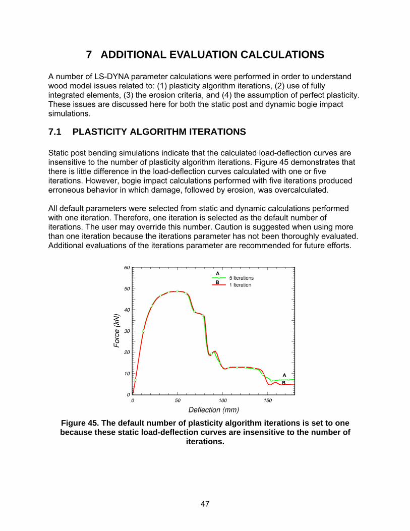
47

7 ADDITIONAL EVALUATION CALCULATIONS A number of LS-DYNA parameter calculations were performed in order to understand wood model issues related to: (1) plasticity algorithm iterations, (2) use of fully integrated elements, (3) the erosion criteria, and (4) the assumption of perfect plasticity. These issues are discussed here for both the static post and dynamic bogie impact simulations.

7.1 PLASTICITY ALGORITHM ITERATIONS Static post bending simulations indicate that the calculated load-deflection curves are insensitive to the number of plasticity algorithm iterations. Figure 45 demonstrates that there is little difference in the load-deflection curves calculated with one or five iterations. However, bogie impact calculations performed with five iterations produced erroneous behavior in which damage, followed by erosion, was overcalculated. All default parameters were selected from static and dynamic calculations performed with one iteration. Therefore, one iteration is selected as the default number of iterations. The user may override this number. Caution is suggested when using more than one iteration because the iterations parameter has not been thoroughly evaluated. Additional evaluations of the iterations parameter are recommended for future efforts.

Figure 45. The default number of plasticity algorithm iterations is set to one because these static load-deflection curves are insensitive to the number of

iterations.

48

7.2 FULLY INTEGRATED ELEMENTS The static post peak-load deflection comparisons previously shown in figure 27 indicate that the fully integrated S/R (type 2 eight-point integration) elements produce a more brittle behavior than the standard under-integrated elements. This is probably because the fully integrated elements erode when just one of the eight integration points fails. By failure, we mean that the wood material model calculates a 99.9-percent reduction in stiffness and strength (in all six stress components both parallel and perpendicular to the grain) at that integration point. Therefore, seven of the eight integration points could still be loaded in tension when the element erodes. As a check, static bending calculations were performed with and without erosion using both the standard and fully integrated elements (as shown in figure 46). There is essentially no difference between the responses calculated with and without erosion when standard elements are used (not shown). However, some difference is calculated when fully integrated elements are used. This indicates that the fully integrated elements are eroding prematurely (while still carrying load). One possible consequence of premature erosion is a fracture energy that is mesh-size sensitive and problem-dependent.

Figure 46. Erosion affects the fully integrated element curves, but not the under-

integrated element curves, indicating that the fully integrated elements erode while still carrying load.

Roadside safety applications are primarily dynamic, so bogie impact simulations were also performed with fully integrated elements in the breakaway region for comparison with under-integrated elements. Deformed configurations with damage fringes are shown in figure 47. Energy-deflection and velocity-reduction histories are shown in figure 48. The damage fringes and histories calculated with eight-point integration are similar to those calculated with single-point integration. These bogie impact simulations suggest that eight-point integration can currently be used in the breakaway region of bogie impact simulations; however, analysts are urged to use it with caution. Preliminary

49

calculations performed with eight-point integration in the impact region simulate excessive erosion. Therefore, use of eight-point integration in the impact region is not currently recommended.

C

(a) With eight-point integration (b) With one-point integration

Figure 47. Deformed configurations and fringes of damage calculated with fully integrated elements (eight points) are similar to those calculated with under-

integrated elements (one point).

(a) Energy versus deflection (b) Velocity versus time

Figure 48. Energy-deflection and bogie velocity-reduction histories are not strongly influenced by the type of element formulation (eight points or one point)

modeled in the breakaway region.

50

7.3 EROSION CRITERIA Checks were also performed on the erosion criteria. As the default setup, elements erode when failure occurs parallel to the grain because all six components of stress are degraded to near zero. Elements do not erode when failure occurs perpendicular to the grain because only three components of stress (perpendicular to the grain) are degraded to near zero. The parallel-to-the-grain stress components are not degraded with perpendicular damage. Thus, the element is still able to carry load parallel to the grain after perpendicular failure occurs. All default parameters were selected from static and dynamic calculations performed with the default erosion criteria. As an option, a flag is included to request erosion once perpendicular-to-the-grain failure occurs. For simplicity, this flag is called the perpendicular erosion flag and this erosion option is referred to as perpendicular erosion. Both static and dynamic simulations were performed with and without perpendicular erosion. The static calculations are discussed first, followed by the dynamic calculations. Static deformed configurations and load-deflection curves are shown in figures 49 and 50, respectively, for calculations performed with and without perpendicular erosion. The deformed configuration calculated with perpendicular erosion is more realistic than the deformed configuration calculated without perpendicular erosion. To see the perpendicular damage in the calculation without perpendicular erosion, one can look at damage fringes (as shown in figure 49(c)). Red denotes elements with damage levels of d > 0.80, blue denotes elements with a damage range of 0.60 < d < 0.80, and cyan denotes elements with a damage range of 0.40 < d < 0.60. Perpendicular erosion also has a minor effect on the static load-deflection curves. The post-peak softening behavior calculated with perpendicular erosion is slightly more brittle than that calculated without perpendicular erosion (figure 50). Dynamic deformed configurations and load-deflection curves are shown in figures 51 and 52, respectively, for calculations performed with and without perpendicular erosion. As similarly noted for the static simulations, the breakaway region calculated dynamically with perpendicular erosion looks more realistic than that calculated without perpendicular erosion. However, slight erosion is also calculated in the impact region even though no visible damage was reported in the tests. Perpendicular erosion has little demonstrated effect on the load-deflection curves.

51

(a) Without perpendicular (b) With perpendicular (c) Fringes of damage erosion erosion

Figure 49. The breakaway region calculated with perpendicular erosion in these static bending simulations looks more realistic than that calculated without

perpendicular erosion; however, perpendicular erosion is not recommended for practical use.

Figure 50. Load-deflection curves calculated with perpendicular erosion are

slightly more brittle than those calculated without perpendicular erosion.

52

C

(a) With perpendicular erosion (b) Damage fringes without

perpendicular erosion Figure 51. The breakaway region calculated with perpendicular erosion in this

bogie impact simulation looks more realistic than that calculated without perpendicular erosion.

(a) Energy versus deflection (b) Velocity versus time

Figure 52. Dynamic load-deflection and bogie velocity-reduction curves calculated with perpendicular erosion are nearly identical to those calculated

without perpendicular erosion. In fact, in some cases, perpendicular erosion can have an unrealistic effect on the calculated response. Some preliminary calculations performed with the simplest elastic bogie (without neoprene on the cylinder) simulated excessive erosion in the impact

53

region. One such calculation is demonstrated in figure 53. One possible approach is to request perpendicular erosion in the breakaway region, but not request it in the impact region. Therefore, perpendicular erosion is not the default option (it must be specifically requested), nor is it recommended for general use.

C

Figure 53. Use of perpendicular erosion causes excessive erosion to be

calculated in the impact region in this preliminary bogie impact calculation.

7.4 POST-PEAK HARDENING PARAMETER The default behavior of the wood model is perfectly plastic in both parallel- and perpendicular-to-the-grain compression. This means that there is no increase or decrease in strength with increasing strain. Perfectly plastic behavior was previously demonstrated in figure 1(c). The FPL clear wood and timber compression data previously analyzed in figures 3 and 5 exhibit perfect plasticity, at least for perpendicular strains as great as 4 percent. However, parallel strains of 20 to 30 percent are typically calculated at ground level in the compressive region of the post in the bogie impact calculations. Recent uninstrumented, unconfined compression tests of pine samples conducted by the user indicate softening at large strain parallel to the grain and hardening perpendicular to the grain. Post-peak softening in compression (parallel or perpendicular) is not currently available in the wood material model. Although the damage model (which is responsible for softening) is applied to the stresses in compression, the stresses do not soften, because a compressive fracture energy of infinity is assumed. Fracture energy in compression is not currently an input value (as it is for tension and shear). Infinite

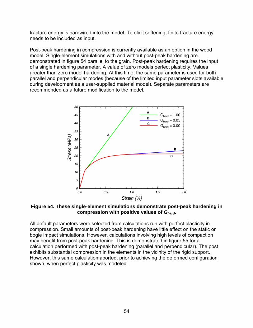
54

fracture energy is hardwired into the model. To elicit softening, finite fracture energy needs to be included as input. Post-peak hardening in compression is currently available as an option in the wood model. Single-element simulations with and without post-peak hardening are demonstrated in figure 54 parallel to the grain. Post-peak hardening requires the input of a single hardening parameter. A value of zero models perfect plasticity. Values greater than zero model hardening. At this time, the same parameter is used for both parallel and perpendicular modes (because of the limited input parameter slots available during development as a user-supplied material model). Separate parameters are recommended as a future modification to the model.

Figure 54. These single-element simulations demonstrate post-peak hardening in

compression with positive values of Ghard. All default parameters were selected from calculations run with perfect plasticity in compression. Small amounts of post-peak hardening have little effect on the static or bogie impact simulations. However, calculations involving high levels of compaction may benefit from post-peak hardening. This is demonstrated in figure 55 for a calculation performed with post-peak hardening (parallel and perpendicular). The post exhibits substantial compression in the elements in the vicinity of the rigid support. However, this same calculation aborted, prior to achieving the deformed configuration shown, when perfect plasticity was modeled.

55

C

Figure 55. Inclusion of post-peak hardening, both parallel and perpendicular to the grain, prevented this calculation from aborting at a large deflection.

Recommendations for future efforts include laboratory compression measurements and wood model enhancements. The laboratory compression measurements should include stress displacement and fracture energy for clear wood and graded wood samples, both parallel and perpendicular to the grain. These measurements should be made as a function of moisture content. If these measurements show softening, as recently measured parallel to the grain, then model enhancements should proceed. The wood model enhancements should include an input slot for compressive fracture energy; smooth variation of the fracture energy between compression, shear, and tension; and identification of default compressive fracture energy values as a function of moisture content. If these measurements show hardening, as recently measured perpendicular to the grain, then the existing post-peak hardening model should be evaluated for accuracy and for selection of default post-peak hardening parameters. Some porous materials exhibit substantial stiffening at high strain levels (70 to 80 percent) after all pores are compacted, which is called lockup. The current post-peak hardening formulation does not model lockup. The need for a lockup model should be assessed with regards to roadside safety applications.

57

8 DEVELOPER’S SUMMARY AND RECOMMENDATIONS A wood material model was developed, implemented into the LS-DYNA finite element code, and evaluated for use in roadside safety applications. Eight evaluation calculations (four quasi-static and four dynamic) were performed by the developer with the results documented in chapters 1 through 7 of this report. The main evaluation calculations were dynamic bogie impact at 9.6 m/s into southern yellow pine (grade 1 unfrozen, grade 1 frozen, and DS-65 unfrozen) and Douglas fir (grade 1) posts. The wood model calculates post breakage just below ground level (in agreement with the measured breakage locations). The wood model also calculates bogie kinetic energy and velocity reductions that are in reasonable agreement with final measured quantities. However, the evaluation calculations indicate some limitations in both the test data and model formulation. Recommendations for future efforts, based on these limitations, are itemized here. These enhancements are not required for achieving good correlation between the wood model and post data.

1. Parallel Fracture Energy: Perform quasi-static tensile tests of clear wood specimens to directly measure the parallel-to-the-grain fracture energy as a function of moisture content.

Fracture energy is the area under the stress-displacement curve from peak stress to zero stress, measured during unconfined tension tests conducted parallel to the grain. Parallel fracture energy is an important input parameter whose value has a strong effect on post response in bogie impact and static bending simulations. Although the suite of FPL clear wood pine data implemented into the wood model as default properties is quite extensive, it does not include fracture energy measurements. Therefore, correlations with bogie impact and static bending test data were used to set the default fracture energies. However, the parallel fracture energy selected from the static bending correlations is five times greater than that selected from the bogie impact correlations. This should be clarified. A minimum of 15 quasi-static tensile tests of clear wood pine are recommended in order to develop quadratic equations for parallel fracture energy as a function of moisture content. These tests should be conducted at five moisture content levels, with each test repeated three times. Additional tests conducted on grade 2 and DS-65 pine would provide information on the variation of fracture energy as a function of grade. Dynamic tensile tests (e.g., at 0.1 or 1.0 s-1 (a typical strain rate in the post)) would also provide useful information on the variation of fracture energy with strain rate.

2. Perfect Plasticity: Perform quasi-static compression tests of clear and graded

wood pine specimens to moderate compression levels to evaluate the assumption of perfect plasticity in compression.

58

The wood material model simulates perfectly plastic behavior in compression both parallel and perpendicular to the grain (as the default behavior). An option is also included to model post-peak hardening in compression; however, no option is included to model softening in compression.

FPL conducted a suite of laboratory compression tests on clear wood samples for strain levels up to about 4 percent that were used to set the model behavior. The measured stress-strain data indicate that perfect plasticity is a reasonable assumption (at least for strains up to 4 percent). However, parallel strain levels up to 30 percent are noted in the bogie impact simulations. Therefore, the user conducted a few quick-look compression tests of graded pine specimens for strains up to 90 percent. Their measured stress-strain data indicate softening parallel to the grain and hardening perpendicular to the grain.1 Future efforts could generate hardening and/or softening data for wood in compression to moderate strain levels (about 30 percent). A suite of tests are recommended for clear wood and two grades of saturated pine (grade 1 and DS-65) to obtain plots of load versus axial and lateral deflection for strains up to 30 percent. Tests should be conducted both parallel and perpendicular to the grain as a function of moisture content. If a review of the test data indicates that softening is evident, then a compressive softening formulation is recommended for implementation, which may or may not affect post fracture. It is not clear to the developer that a compressive softening formulation is needed or that it would enhance post fracture behavior.

3. Quality Factors: Perform static tensile and compression tests of dry, partially

saturated, and saturated pine to determine how quality factors vary as a function of moisture content.

The suite of pine data implemented into the wood model as default properties is for clear wood, whereas real posts are graded wood such as grades 2, 1, or DS-65. Clear wood is stronger than graded wood. The approach for setting default properties for graded wood is to apply quality factors (strength-reduction factors) to the clear wood to account for reductions in strength as a function of grade. Two quality factors are set. One quality factor is applied to the tensile and shear strengths, the other is applied to the compressive strengths. Default quality factors are estimated from correlations of calculations with static bending test data. However, the quality factors estimated from simulations of the user’s saturated-post bending tests are about twice as high as those estimated from the simulation of FPL’s partially saturated timber-bending tests. This suggests that quality factors vary as a function of moisture content. Quality

1The measured hardening behavior perpendicular to the grain was unexpected. It looked similar to the behavior of the isotropic porous materials in uniaxial strain, not uniaxial stress. This unexpected behavior may be because wood is orthotropic.

59

factors currently implemented in the model as default properties are those from the saturated-post correlations. Static tests (compression and tension) of graded wood are recommended at a minimum of three moisture content levels in order to develop quadratic equations for quality factors as a function of moisture content. Conducting compression and tension tests, rather than bending tests, would isolate the tensile quality factors from the compressive factors. A related issue is whether the same quality factors should be applied perpendicular to the grain as those applied parallel to the grain, as is the current default implementation (although an option is available to neglect quality factors perpendicular to the grain). If possible, tests should be conducted both parallel and perpendicular to the grain.

4. Coupling Between Parallel and Perpendicular Modes: Evaluate and enhance the parallel and perpendicular yield surface and plasticity formulations to include coupling between the parallel and perpendicular modes. Evaluation of such coupling would require measurement of the volume expansion/contraction (effective Poisson’s ratio in the plastic region) behavior of wood.

One theoretical limitation of the wood model is that there is no coupling between the parallel and perpendicular modes in the plastic region. Such coupling affects volumetric behavior. The suite of clear wood data provided by FPL included measurement of the major Poisson’s ratio in the elastic region. Typical values are around νLT = 0.16 for pine at the fiber saturation point. No measurements were reported for the effective Poisson’s ratio in the plastic/damage regions (once the material yields or softens). The effective Poisson’s ratio is the ratio of the lateral strain to the axial strain in uniaxial stress tests (without lateral confinement). Porous materials tend to flow during yielding and softening, which can result in an effective Poisson’s ratio that is larger or smaller than the elastically measured value. For example, for porous geological materials such as concrete, the effective Poisson’s ratio is typically modeled as being greater than the elastic ratio in unconfined compression (with values greater than 1) and less than the elastic ratio in unconfined tension.

The user has examined the behavior of the wood model for single elements of pine in unconfined tension. An increase in the volume of the element was noted. The user believes that there should be no change in the volume of wood in tension (i.e., wood is incompressible). To achieve no change in volume, the elastic and effective Poisson’s ratios would have to be 0.5. The FPL data indicate that the elastic Poisson’s ratio parallel to the grain is not 0.5. However, no lateral strain or change in volume measurements is available to confirm or refute an effective Poisson’s ratio of 0.5 in the plastic region. Therefore, we recommend that all additional test data generated should include lateral strain measurements. The unconfined compression and tension tests recommended in items 2 and 3 above should include measurement of both axial and lateral strain.

60

Setting the compressibility or effective Poisson’s ratio behavior of the wood model is not simply a matter of specifying an input value, rather, it requires that changes be made to the formulation of the model to include coupling between the parallel (axial) plasticity and perpendicular (lateral) plasticity. The current wood model includes separate yield surfaces and plasticity computations for yielding parallel and perpendicular to the grain. As a result, yielding parallel to the grain does not induce plastic flow perpendicular to the grain. Similarly, yielding perpendicular to the grain does not include plastic flow parallel to the grain. We recommend exploring and implementing methods of coupling the plastic flow once sufficient test data are generated to set the coupling via measurement of the effective Poisson’s ratio or volume change. This could be done regardless of whether or not the tests indicate incompressibility.

5. Erosion Method: All erosion criteria could be enhanced to be user-specified,

including the damage-based criteria. Future efforts could also include modifications, additions, and/or elimination of the distorted element checks and possible inclusion of an input flag to turn these checks on and off.

The primary erosion mechanism is based on damage. Element erosion, by default, is based on parallel damage in excess of 99 percent. Erosion, by option, may also be based on perpendicular damage in excess of 98.9 percent. As element damage approaches 99 percent, strength and stiffness approach 1 percent of their original values. Elements with nearly zero strength and stiffness could possibly experience shooting nodes and drastically deform, invert, expand, or contract in response to very small loads. Such behavior can cause a calculation to abort. Element erosion is a technique that prevents the calculation from aborting by removing these elements from the calculation before large distortions occur. Erosion also provides a good visual image of breakage in the damage region. Because elements do not automatically erode with perpendicular damage, the model includes a check on the maximum strains perpendicular to the grain to determine whether they are greater than 90 percent. If so, the element erodes if perpendicular damage has already exceeded 98 percent.

In addition to the damage-based erosion criteria, a number of checks are implemented in the model to prevent highly distorted elements from causing computational problems. These distorted element checks were implemented for the explicit purpose of debugging the model during use of the user-defined material model interface and do not necessarily need to be retained in the final model. They include: • A check on the element volume to determine whether it is less than zero. • A check on the current relative volume to determine whether it is less than

10 percent.

61

• A check on the maximum strain increment to determine whether it is greater than 1 percent.

Element erosion will occur if any of these conditions are met.

6. Mesh-Size Dependency: Future efforts could include direct-pull and unconfined compression simulations of wood specimens at different mesh refinements to demonstrate mesh-size response. The issue here is to isolate the material response without the complicating effects of other materials and contact issues.

A related issue that is recommended for evaluation is whether to use the initial element length or the updated element length in the calculation of the damage parameter. The updated element length is currently implemented. Damage is based on element length in an effort to regulate mesh-size sensitivity.

7. Iterations Parameter: Evaluate and enhance the plasticity algorithm iterations

method.

The plasticity algorithm returns the stress state to the yield surface if the elastic stress state is predicted to lie outside the yield surface. The purpose of the iterations parameter is to increase the accuracy of the return through iteration and subsequent tolerance checks to ensure that the stress state lies on the yield surface. Static calculations indicate that one iteration is just as accurate as five iterations. In contrast, bogie impact simulations calculate excessive damage and erosion with five iterations. Therefore, the default number of iterations has been set to one. Future model enhancements should include debugging of the iterations parameter for dynamic applications.

8. Accelerometer Measurements: Perform future bogie impact tests with

measurements made on the post rather than on the bogie.

The force-deflection and energy-deflection performance envelopes from the user’s bogie impact tests are measurements processed from an accelerometer located at the center of the bogie frame. The high-frequency measurements are filtered to produce a smooth signal. Because all measurements are made on the bogie rather than on the post, good correlations between the calculations and the processed data require an accurate bogie model (geometric and material) as well as an accurate wood post model. Calculations completed to date indicate that the computed bogie accelerations strongly depend on the bogie model type (rigid or elastic) and output sampling rate. For example, the calculated bogie acceleration (force) histories contain a higher frequency content than that measured. The calculated histories are also more oscillatory than those measured. On the other hand, computed force histories derived from cross-sectional forces in the post are much less sensitive to the sampling rate and bogie model type than those derived from the bogie

62

accelerometer location. This suggests that measurements recorded directly on the post would isolate wood performance and facilitate evaluation of the wood model. Instrumenting the wood posts could prove to be a challenging endeavor.

9. Boundary Conditions: Perform future static and bogie impact tests on posts with well-defined boundary conditions.

Posts are typically situated in highly deformable media, such as soil. Therefore, static and bogie impact tests were intended to be conducted under fixed-base conditions. The posts in the static tests were placed in a rigid base with steel and neoprene shims to wedge the post into the support. The posts in the dynamic tests were loosely placed in a steel tube in the ground and wedged in with neoprene and plywood shims. LS-DYNA results calculated with simple (post nodal constraints) to sophisticated (support and neoprene modeled explicitly) meshes produce different computational results. Performing future tests with simple, easy-to-model boundary conditions would help with future evaluation of the wood model.

63

9 USER'S INTRODUCTION The calculations and conclusions of chapters 9 through 16 were conducted and documented by the user. Several finite element models were developed throughout the validation effort, including single-element models for tension and compression, a cube crushing model, several static wood post testing models, and a dynamic wood post testing model. As a first step in the simulation validation effort, the user successfully reproduced results obtained by the developer on the user’s computers. Next, the user applied the new wood material model to several different methods not attempted by the developer. Several areas of concern were revealed at this stage. These concerns are documented throughout chapters 9 through 16. The majority of the simulations reported in this document were performed using LS-DYNA, version 970, revision 1812, compiled on June 7, 2002, on both PC Windows and SGI® UNIX-based machines. All areas of concern listed in this report were tested on this latest version of the wood model.

65

10 VALIDATION CRITERIA FOR THE WOOD MATERIAL MODEL

To validate the wood material model, several criteria must first be developed in order to determine whether the model is working as desired. To this end, the validation process at the user’s facility consisted of verifying that the results were similar on different computer platforms (chapter 11) by simulating single-element models in order to check basic fundamental behavior (chapter 12), simulating static wood post tests (chapter 13), simulating dynamic wood post tests (chapter 14), checking the sensitivity of the simulation models by varying numerous parameters (throughout chapters 12, 13, and 14), and by simulating wood-cube crushing tests performed in parallel with this project. Because of time constraints, the cube crushing test and simulation were not revisited in this final report. Interested readers are urged to contact the user for details.

10.1 NDOR TESTS: PERFORMANCE ENVELOPES In 1995, the user ran a series of static and dynamic post testing for the Nebraska Department of Roads (NDOR). The series consisted primarily of 152.4-mm by 203.2-mm by 1828.8-mm (6-inch by 8-inch by 72-inch) southern yellow pine of various grades and ages. The wood posts were obtained from previously installed guardrail systems throughout Nebraska. A smaller series of dynamic tests using frozen southern yellow pine and Douglas fir wood posts were also conducted. Data collected from the 1995 NDOR project were to be used for validating the wood material model. Based on several meetings and discussions, the simulation user community requested that the wood material model have specific options for selecting southern yellow pine of grades DS-65 and 1/1D (among other options). In order to validate the material model for those specific cases, the 1995 NDOR data were completely analyzed to determine the appropriate tests with which to compare the simulation results. The details for the results of this analysis are not presented herein; however, interested readers are urged to contact the user for details. Grades 1 and 1D wood post test results showed very little difference in behavior; thus, this report will use the terminology of grade 1 to represent the combined grades 1 and 1D. Performance envelopes were constructed using the most typical behavior of the desired wood and grades for both static and dynamic test conditions (see figure 56). Force-deflection and energy-deflection results from the simulations would need to fall within the performance envelopes in order to be considered validated. Photographs from the testing are presented in figures 57 through 61.

66

(c) Grade DS-65 energy (d) Grade 1 energy

Figure 56. Performance envelopes from 1995 NDOR testing.

(a) Grade DS-65 force (b) Grade 1 force

67

Figure 57. Static post setup. (a) Post and bogie vehicle (b) Post

Figure 58. Dynamic post setup.

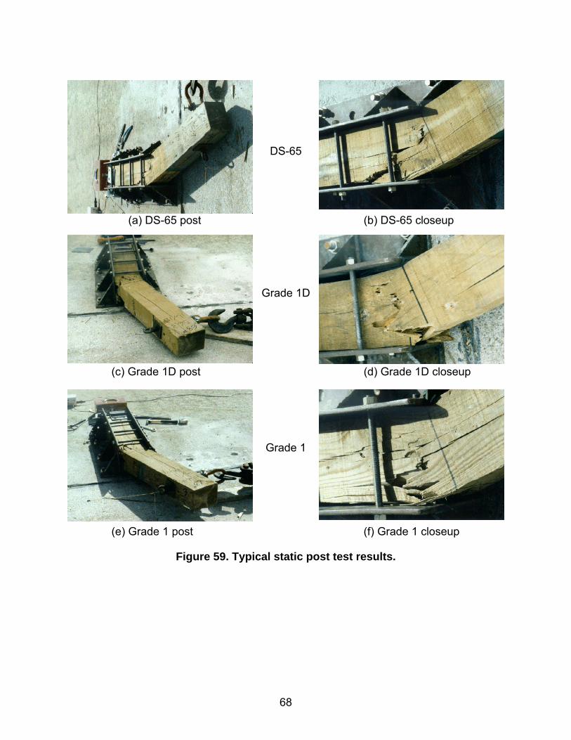
68

DS-65 Grade 1D Grade 1

Figure 59. Typical static post test results.

(a) DS-65 post (b) DS-65 closeup

(c) Grade 1D post (d) Grade 1D closeup

(e) Grade 1 post (f) Grade 1 closeup

69

DS-65

Grade 1D

Grade 1

Figure 60. Typical dynamic post test results.

(a) DS-65 breakage

(c) Grade 1D breakage

(e) Grade 1 breakage

(b) DS-65 post

(d) Grade 1B post

(f) Grade 1 post

70

(a) Clean break

(b) Atypical behavior

Figure 61. Other dynamic post test results.

71

11 VERIFICATION OF RESULTS ON DIFFERENT COMPUTER PLATFORMS

In this section, a comparison of three different types of models using the developer’s wood model in LS-DYNA is made using different computer platforms. The results from an Intel®-based PC (using Windows) are provided by the developer, while the results from an SGI Octane® (using UNIX) are provided by the user. Although the results are shown to be somewhat different on the different computer platforms, they are considered to be within an acceptable range based on previous experiences using different computers. This phenomenon is well known and is documented in the LS-DYNA user’s manual. It is a computer platform issue and not a software issue. The models discussed in this section are good for verifying the accuracy of the codes between computer platforms, but are shown to be unacceptable for validating the wood model itself as an accurate material for modeling wood in roadside hardware applications. However, investigating the wood material model itself is left for the remaining sections of this report.

11.1 SINGLE-ELEMENT MODELS Four single-element models were run to check the consistency between PC (Intel)-based computers and SGI-based computers. The specific results for each model are described in tables 4, 5, 6, and 7 below. In general, for single-element models, PC and SGI computers give equivalent results. Material summaries (matsum) and global statistics (glstat) were consistent throughout. Also, displacements were consistent throughout.

Table 4. Model Cfa: Uniaxial Compression in Parallel Direction

Output File Examined Variables Checked Differences Between

Computers d3plot (history) Effective stress No visible differences

glstat Internal energy, kinetic energy, and time-step size No visible differences

Matsum Internal energy and kinetic energy No visible differences

72

Table 5. Model Cfe: Uniaxial Compression in Perpendicular Direction

Output File Examined Variables Checked Differences Between

Computers

d3plot (history) x-stress, z-stress, and pressure No visible differences

Glstat Internal energy, kinetic energy, and total energy No visible differences

Table 6. Model Tfa: Uniaxial Tension in Parallel Direction

Output File Examined Variables Checked Differences Between

Computers

d3hsp Inertial tensor and principal directions

Slight differences for values that are near zero

d3plot (history)

Nodal: x, y, and z displacements Element: plastic strain and stress

No visible differences

Glstat Time-step size No visible differences

Matsum

Internal energy Kinetic energy

No visible differences Slight difference; however, magnitudes are very small (E-6)

Table 7. Model Tfe: Uniaxial Tension in Perpendicular Direction

Output File Examined Variables Checked Differences Between

Computers

d3plot (history) Plastic strain, stress, and pressure No visible differences

Glstat Internal energy and time-step size No visible differences

Matsum Internal energy No visible differences

73

11.2 DYNAMIC POST TEST SIMULATION: BOGIE MODEL This model is a rather detailed model of the dynamic post tests performed at the user’s facility. As evidenced in figures 62 through 67, the results from the developer’s computers match the results from the user’s computers very well for the first 15 ms of simulation. After that time, the results begin to diverge a little with regards to the contact forces and internal energy absorbed by the post (as shown in figures 64 and 66, respectively). Overall, agreement between the results is acceptable. Model Validity: Although the developer and the user are getting nearly the same results for this model, the model itself is unacceptable for evaluating the validity of the wood model. This is because the contact between the wood and the neoprene-lined concrete sleeve is not behaving appropriately (as shown in figure 68). The interpenetration of the neoprene into the wood causes a local lockup that prevents the post from sliding along that edge. Developer’s Results User’s Results

Figure 62. Impact sequence of post simulation.

(a) 0 ms (developer) (b) 10 ms (developer) (c) 30 ms (developer)

(d) 0 ms (user) (e) 10 ms (user) (f) 30 ms (user)

74

(a) Developer’s results

(b) User’s results

Figure 63. Damage (stored as effective plastic strain in d3plot files).

75

Figure 64. Contact forces. Figure 65. Cross section at ground level. Figure 66. Energy of post parts. Figure 67. Bogie velocity.

Figure 68. Contact penetrations caused locking of parts.

[ms]

X-fo

rce

[kN

]

76

11.3 DYNAMIC POST TEST SIMULATION: FAST BOGIE MODEL The fast bogie model is a simplification of the bogie model described above. This model was generated by the developer to speed up the calculation time. As evidenced in figures 69 through 71, the results from the developer’s computers match the results from the user’s computers very well for the first 10 ms of simulation. After that time, the results begin to diverge. Overall, agreement between the results is acceptable, considering the crudeness of the model. Model Validity: Because of the excessive bending of the post without total fracture at ground level, this model is considered to be unacceptable for evaluating the validity of the wood model.

Figure 69. Sequence of fast bogie simulations.

(e) 40 ms (developer) (f) 40 ms (user)

(a) 0 ms (developer)

(c) 10 ms (developer)

(b) 0 ms (user)

(d) 10 ms (user)

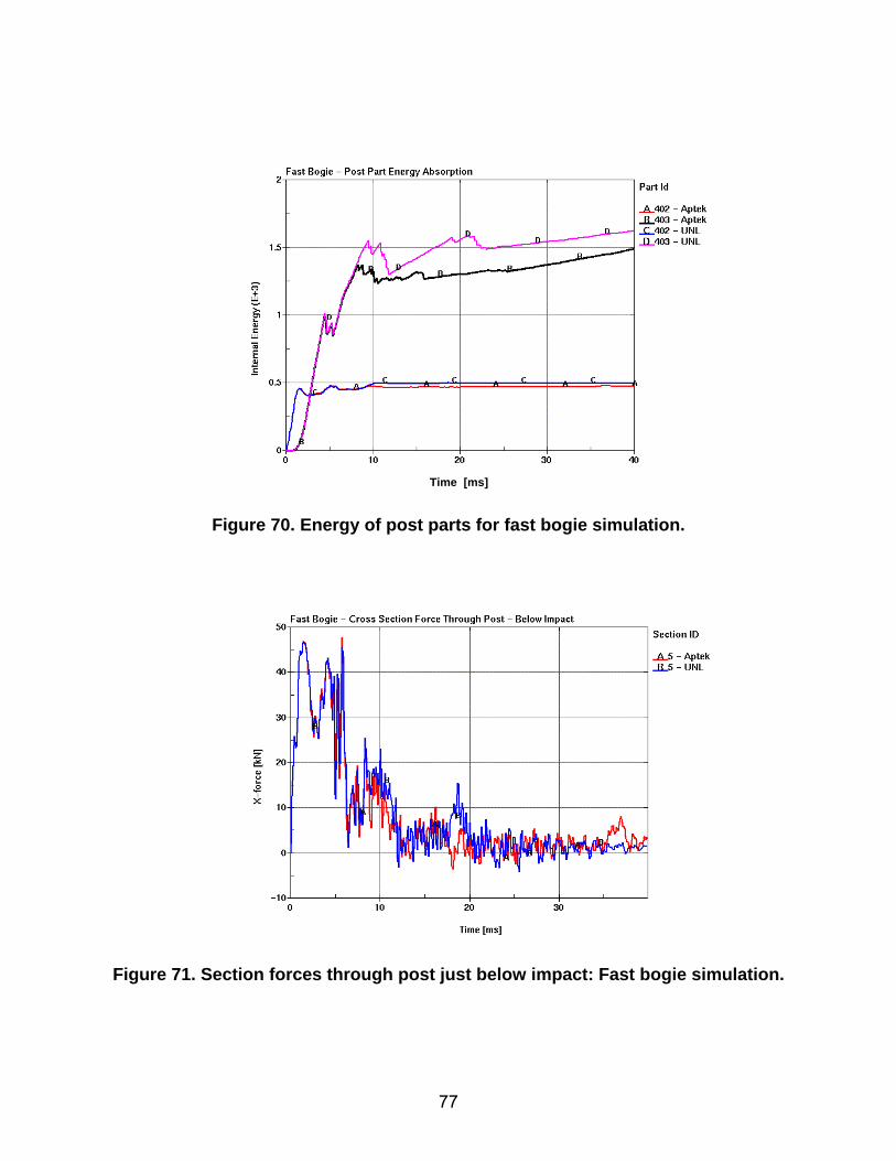
77

Figure 70. Energy of post parts for fast bogie simulation. Figure 71. Section forces through post just below impact: Fast bogie simulation.

Time [ms]

79

12 SINGLE ELEMENT: TENSION PARALLEL TO THE GRAIN A single solid element is used to study the developer’s wood material model in uniaxial tension parallel to the grain. Specifically, a parameter study investigating the southern yellow pine option is performed. The parameters investigated are wood grade, moisture content, and temperature. Stress-strain curves, volume-time curves, and changes in the 29 wood parameters (as reported in the d3hsp file) are presented. The stress-strain behavior of the single element in tension is as desired. In all cases, stress increases linearly with respect to strain until a peak strength is reached, followed by a gradual decrease in stress as the material undergoes damage and eventually fails. With respect to wood grade, increasing strength is observed as the grade is improved. With respect to moisture content, fully saturated wood is relatively weak, but ductile. As the moisture content decreases, the material becomes stronger and more brittle. When the wood becomes very dry, the strength decreases, yet maintains a brittle behavior. With respect to temperature, low-temperature pine is relatively strong, yet brittle, while wood at a high temperature is relatively weak and ductile. The volume of the single elements in tension parallel to the grain uniformly increases during all simulations by as much as 6 percent. This is an unexpected and undesirable result because it is believed by the user that, at a minimum, volume should be conserved for wood. A significant example of this volume expansion is shown in chapter 14 of this report. Because of time limitations, various other single-element simulations were not performed, but are recommended (including compression, shear, and torsion loading both parallel and perpendicular to the grain).

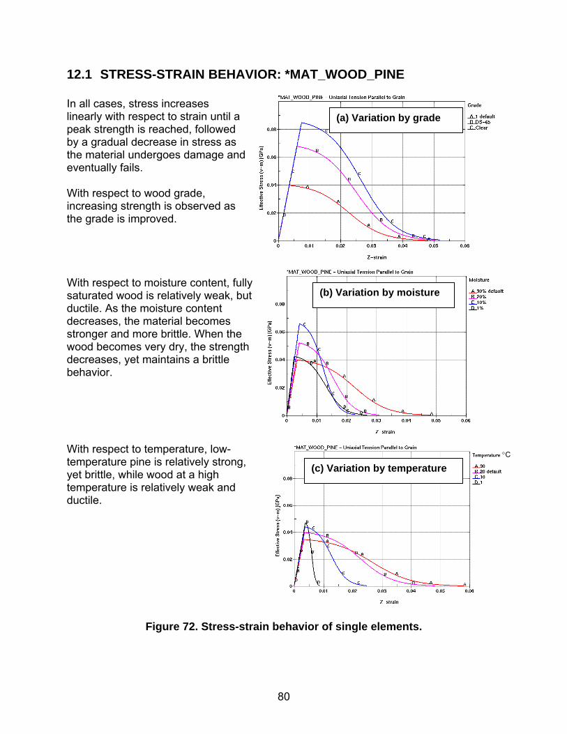
80

12.1 STRESS-STRAIN BEHAVIOR: *MAT_WOOD_PINE In all cases, stress increases linearly with respect to strain until a peak strength is reached, followed by a gradual decrease in stress as the material undergoes damage and eventually fails. With respect to wood grade, increasing strength is observed as the grade is improved. With respect to moisture content, fully saturated wood is relatively weak, but ductile. As the moisture content decreases, the material becomes stronger and more brittle. When the wood becomes very dry, the strength decreases, yet maintains a brittle behavior. With respect to temperature, low-temperature pine is relatively strong, yet brittle, while wood at a high temperature is relatively weak and ductile.

Figure 72. Stress-strain behavior of single elements.

(a) Variation by grade

(b) Variation by moisture

(c) Variation by temperature °C

81

12.2 VOLUME OF ELEMENT: *MAT_WOOD_PINE The volume of the single element in tension parallel to the grain uniformly increases during all simulations by as much as 6 percent. This is an unexpected and undesirable result because it is believed by the user that, at a minimum, volume should be conserved for wood. A significant example of this volume expansion is shown in chapter 14 of this report. Note: The drop-off of volume on curves is where failure of the element occurs.

Figure 73. Volumetric behavior of single elements.

(a) Variation by grade

(b) Variation by moisture

Volu

me

[mm

3 ] (E+

3)

Volu

me

[mm

3 ] (E+

3)

Volu

me

[mm

3 ] (E+

3)

°C

(c) Variation by temperature

Time [ms]

82

12.3 MATERIAL PROPERTIES: *MAT_WOOD_PINE When using the *MAT_WOOD_PINE option, the user specifies parameters such as wood grade, moisture content, and temperature. However, the underlying wood material model is based on a large set of theoretical parameters. By setting the wood grade, for example, the underlying parameters are modified appropriately. This section provides a set of tables (tables 8, 9, and 10) that record the variations in the underlying parameters based on changing a single parameter.

Table 8. Parameters based on wood grade. Single Solid Element – Uniaxial Tension Parallel to the Grain Units kg, mm, ms, kN, GPa Density 6.731E-07 kg/mm3

*MAT_WOOD_PINE Default Parameters Except for Grade

Stiffmess: Grade 1 (default)

Grade DS-65 Grade Clear

EL Parallel Normal Modulus 11.350000 ET Perpendicular Normal Modulus 0.246800 GLT Parallel Shear Modulus 0.715200 GLR Perpendicular Shear Modulus 0.087510 PR Parallel Major Poisson’s Ratio 0.156800 Strength: Xt Parallel Tensile Strength 0.040030 0.068130 0.085160 Xc Parallel Compressive Strength 0.013320 0.019670 0.021150 Yt Perpendicular Tensile Strength 0.000963 0.001640 0.002050 Yc Perpendicular Compressive Strength 0.002571 0.003796 0.004082 Sxy Parallel Shear Strength 0.004275 0.007277 0.009096 Syz Perpendicular Shear Strength 0.005985 0.010190 0.012730 Damage: Gf1 Parallel Fracture Energy in Tension 0.020050 0.034130 0.042660 Gf2 Parallel Fracture Energy in Shear 0.041480 0.070610 0.088260 Bfit Parallel Softening Parameter 30.000000 Dmax Parallel Maximum Damage 0.999900 Gf1 Perpendicular Fracture Energy in Tension 0.000401 Gf2 Perpendicular Fracture Energy in Shear 0.000830 Dfit Perpendicular Softening Parameter 30.000000 Dmax Perpendicular Maximum Damage 0.990000 Rate Effects: Flpar Parallel Fluidity Parameter: Tension/Shear 0.000 Flparc Parallel Fluidity Parameter: Compression 0.000 Pow_par Parallel Power 0.000 Flper Perpendicular Fluidity Parameter: Tension/Shear 0.000 Flperc Perpendicular Fluidity Parameter: Compression 0.000 Pow_per Perpendicular Power 0.000 Hardening: Npar Parallel Hardening Initiation 0.500 Cpar Parallel Hardening Rate 1008.000 462.500 400.000 Nper Perpendicular Hardening Initiation 0.400 Cper Perpendicular Hardening Rate 252.000 115.600 100.000 Note: Only those values that changed because of the change in grade are provided in the table.

83

Table 9. Parameters based on moisture content. Single Solid Element – Uniaxial Tension Parallel to the Grain Units kg, mm, ms, kN, GPa Density 6.731E-07 kg/mm3

*MAT_WOOD_PINE Default Parameters Except for Moisture Content (MS)

Stiffness:

MC = 30% (default)

MC = 20%

MC = 10% MC = 1%

EL Parallel Normal Modulus 11.350000 12.560000 15.490000 16.720000 ET Perpendicular Normal Modulus 0.246800 0.461900 0.910100 0.959700 GLT Parallel Shear Modulus 0.715200 0.736900 0.789800 0.811900 GLR Perpendicular Shear Modulus 0.087510 0.165500 0.332300 0.349300 PR Parallel Major Poisson’s Ratio 0.156800 0.184200 0.258600 0.303300 Strength: Xt Parallel Tensile Strength 0.040030 0.052380 0.066190 0.042590 Xc Parallel Compressive Strength 0.013320 0.018580 0.037000 0.054760 Yt Perpendicular Tensile Strength 0.000963 0.001458 0.002139 0.001477 Yc Perpendicular Compressive Strength 0.002571 0.003627 0.007145 0.010310 Sxy Parallel Shear Strength 0.004275 0.005577 0.008526 0.009351 Syz Perpendicular Shear Strength 0.005985 0.007808 0.011940 0.013090 Damage: Gf1 Parallel Fracture Energy in Tension 0.020050 0.015660 0.013840 0.011670 Gf2 Parallel Fracture Energy in Shear 0.041480 0.046150 0.050160 0.028480 Bfit Parallel Softening Parameter 30.000000 Dmax Parallel Maximum Damage 0.999900 Gf1 Perpendicular Fracture Energy in Tension 0.000401 0.00313 0.000277 0.000233 Gf2 Perpendicular Fracture Energy in Shear 0.00830 0.000923 0.001003 0.000570 Dfit Perpendicular Softening Parameter 30.000000 Dmax Perpendicular Maximum Damage 0.990000 Rate Effects: Flpar Parallel Fluidity Parameter: Tension/Shear 0.000 Flparc Parallel Fluidity Parameter: Compression 0.000 Pow_par Parallel Power 0.000 Flper Perpendicular Fluidity Parameter: Tension/Shear 0.000 Flperc Perpendicular Fluidity Parameter: Compression 0.000 Pow_per Perpendicular Power 0.000 Hardening: Npar Parallel Hardening Initiation 0.500 Cpar Parallel Hardening Rate 1008.000 Nper Perpendicular Hardening Initiation 0.400 Cper Perpendicular Hardening Rate 252.000 Note: Only those values that changed because of the change in moisture content are provided in the table.

84

Table 10. Parameters based on temperature. Single Solid Element – Uniaxial Tension Parallel to the Grain Units kg, mm, ms, kN, GPa Density 6.731E-07 kg/mm3

*MAT_WOOD_PINE Default Parameters Except for Temperature

Stiffness:

Temperature = 30°C

Temperature = 20°C

(default)

Temperature = 10°C

Temperature = 1°C

EL Parallel Normal Modulus 10.620000 11.350000 11.970000 12.420000 ET Perpendicular Normal Modulus 0.230800 0.246800 0.260200 0.270000 GLT Parallel Shear Modulus 0.668900 0.715200 0.754000 0.782400 GLR Perpendicular Shear Modulus 0.081840 0.087510 0.092250 0.095730 PR Parallel Major Poisson’s Ratio 0.156800 Strength: Xt Parallel Tensile Strength 0.034840 0.040030 0.044370 0.047550 Xc Parallel Compressive Strength 0.011600 0.013320 0.014770 0.015830 Yt Perpendicular Tensile Strength 0.000839 0.000963 0.001068 0.001144 Yc Perpendicular Compressive Strength 0.002238 0.002571 0.002850 0.003055 Sxy Parallel Shear Strength 0.003721 0.004275 0.004739 0.005079 Syz Perpendicular Shear Strength 0.005210 0.005985 0.006634 0.007110 Damage: Gf1 Parallel Fracture Energy in Tension 0.021440 0.020050 0.010460 0.002657 Gf2 Parallel Fracture Energy in Shear 0.044360 0.041480 0.021640 0.005498 Bfit Parallel Softening Parameter 30.000000 Dmax Parallel Maximum Damage 0.999900 Gf1 Perpendicular Fracture Energy in Tension 0.000429 0.000401 0.000380 0.000367 Gf2 Perpendicular Fracture Energy in Shear 0.000887 0.000830 0.000787 0.000758 Dfit Perpendicular Softening Parameter 30.000000 Dmax Perpendicular Maximum Damage 0.990000 Rate Effects: Flpar Parallel Fluidity Parameter: Tension/Shear 0.000 Flparc Parallel Fluidity Parameter: Compression 0.000 Pow_par Parallel Power 0.000 Flper Perpendicular Fluidity Parameter:

Tension/Shear 0.000

Flperc Perpendicular Fluidity Parameter: Compression 0.000 Pow_per Perpendicular Power 0.000 Hardening: Npar Parallel Hardening Initiation 0.500 Cpar Parallel Hardening Rate 1008.000 Nper Perpendicular Hardening Initiation 0.400 Cper Perpendicular Hardening Rate 252.000 Note: Only those values that changed because of the change in moisture content are provided in the table.

85

13 STATIC WOOD POST TEST SIMULATIONS 13.1 STATIC POST MODEL Static post testing consisted of both using neoprene and not using neoprene wedged between the wood post and the braces holding the post. Similar results were obtained with or without the neoprene, so eventually the static tests switched entirely to no neoprene being used for convenience. Because of anticipated contact difficulties with the simulations, two models were made to simulate the physical testing: one model with neoprene and one model without (see figure 74). The area of concern was at the contact interface between the wood post and the edge of the brace. It was thought, and later proven to be true, that the neoprene acted like a softening mechanism between the relatively soft wood post and the rigid clamping frame. However, this effect also proved to be insignificant with regards to the overall post behavior. In the model, the wood post is divided into three parts: (1) part 8001, the loading area on the post; (2) part 8002, the area where the post breaks; and (3) part 8000, the remainder of the post. All three post parts have the same wood material properties. The post is clamped between rigid, fixed braces (part 8004). Loading is supplied to the post through the loading bolt (part 8003) using a prescribed velocity motion of 1 mm/ms. After many different model variations, it was determined that the model without the neoprene could be used for simulating the physical static tests. Some difficulties were encountered while developing the baseline static model. A final model variation was developed that incorporated a rounded edge on the brace (as shown in figure 75). This rounded edge eliminated several contact issues that made the previous models very sensitive to the new wood material model.

Baseline Model A baseline model is established to compare the various static post test simulations. This baseline model uses the default wood material properties for southern yellow pine, which has a grade of 1, a moisture content of 30 percent, and a temperature of 20 degrees Celsius (°C) (*MAT_WOOD_PINE).

86

― Part 8000 (post)

― Part 8001 (post loading area) Part 8003 (loading bolt) ― ― Part 8002 (post breaking area) Part 8008 (neoprene) ―

― Part 8004 (braces)

Part 8006 (steel shim: between brace and post) ― (a) Without neoprene (b) With neoprene

Figure 74. Static post models.

Figure 75. Rounded edge on brace.

87

13.2 BASELINE MODEL VERSUS TEST COMPARISON This section compares baseline simulation results to physical testing for the static post test. The initial behavior of the model is good; however, during fracture, the material model is too weak (as shown in figures 76 and 77 below). The initial fracture strength of the baseline simulation occurs between the minimum and maximum test values. Once the post begins to fracture, simulation forces fall below the minimum force levels seen in testing.

Figure 76. Force deflection: Baseline versus test.

The total fracture energy of the baseline simulation falls below the minimum test value.

Figure 77. Energy deflection: Baseline versus test.

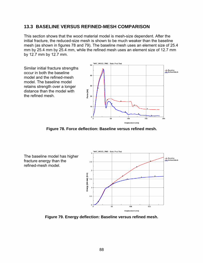
88

13.3 BASELINE VERSUS REFINED-MESH COMPARISON This section shows that the wood material model is mesh-size dependent. After the initial fracture, the reduced-size mesh is shown to be much weaker than the baseline mesh (as shown in figures 78 and 79). The baseline mesh uses an element size of 25.4 mm by 25.4 mm by 25.4 mm, while the refined mesh uses an element size of 12.7 mm by 12.7 mm by 12.7 mm. Similar initial fracture strengths occur in both the baseline model and the refined-mesh model. The baseline model retains strength over a longer distance than the model with the refined mesh.

Figure 78. Force deflection: Baseline versus refined mesh. The baseline model has higher fracture energy than the refined-mesh model.

Figure 79. Energy deflection: Baseline versus refined mesh.

89

Baseline

(a) 29 mm (b) 58 mm (c) 116 mm (d) 189 mm

Refined

(e) 29 mm (f) 59 mm (g) 116 mm (h) 189 mm

Figure 80. Variations by mesh size: Deformed geometry.

90

13.4 PARAMETER STUDY Force-Deflection Behavior: *MAT_WOOD_PINE, Static Post Test Simulation With respect to wood grade, increasing strength is observed as the grade is improved. With respect to moisture content, fully saturated wood is weak, but ductile. As moisture content decreases, the material becomes stronger and more brittle. When the wood becomes very dry, the strength decreases, yet maintains brittle behavior. With respect to temperature, the wood becomes stronger as the temperature decreases.

Figure 81. Force-deflection behavior as a function of grade, moisture content, and temperature.

(a) Variation by grade

(c) Variation by Temperature

(b) Variation by moisture

Forc

e [k

N]

°C

(c) Variation by temperature

91

Energy-Deflection Behavior: *MAT_WOOD_PINE, Static Post Test Simulation With respect to wood grade, fracture energy increases with improved grade. With respect to moisture content, fracture energy varies slightly with changes in moisture content. When wood becomes very dry, fracture energy is reduced significantly. Fracture energy varies slightly with changes in temperature.

Figure 82. Energy-deflection behavior as a function of grade, moisture content, and

temperature.

(a) Variation by grade

(c) Variation by temperature

(b) Variation by moisture

°C

92

1 Default

(a) 29 mm (b) 58 mm (c) 116 mm (d) 189 mm DS-65

(e) 29 mm (f) 58 mm (g) 116 mm (h) 188 mm Clear

(i) 29 mm (j) 58 mm (k) 115 mm (l) 188 mm

Figure 83. Variation by grade: Deformed geometry.

93

30% Default

20% Default

10% Default

1% Default

Figure 84. Variation by moisture content: Deformed geometry.

(a) 29 mm (d) 189 mm (c) 116 mm (b) 58 mm

(e) 29 mm (h) 189 mm (g) 116 mm (f) 58 mm

(i) 29 mm (l) 190 mm (k) 116 mm (j) 59 mm

(m) 29 mm (p) 190 mm (o) 117 mm (n) 59 mm

94

30°C Default

20°C Default 10°C Default

1°C Default

Figure 85. Variation by temperature: Deformed geometry.

(m) 29 mm (p) 189 mm (o) 115 mm (n) 58 mm

(i) 29 mm (l) 189 mm (k) 115 mm (j) 58 mm

(e) 29 mm (h) 189 mm (g) 116 mm (f) 58 mm

(a) 29 mm (d) 188 mm (c) 115 mm (b) 58 mm

95

14 DYNAMIC WOOD POST TEST SIMULATIONS

14.1 DYNAMIC POST MODEL The model used for dynamic post test simulations is shown in figure 86. The bogie impact height is 610 mm (24 inches) above ground level. The impactor on the bogie is modeled with a rigid cylinder wrapped with a deformable neoprene model. The ground is modeled with rigid, fixed solid elements. Deformable neoprene is placed between the ground and the post on both the back and front sides of the post. On the impact side of the post, the neoprene sticks out of the ground approximately 200 mm, while on the other side, the neoprene was slightly below ground level. The dynamic model went through a few modifications. The two primary changes were: (1) the neoprene cover on the cylinder was remeshed to a much finer mesh, and (2) the neoprene used between the ground and the post was also remeshed and sized to match the majority of the testing conditions. Finally, unusual energy problems exhibited on certain hardware platforms with the bogie wheels were fixed by making the wheels rigid (this had no effect on the simulation results). A baseline model was established to compare the various dynamic post test simulations. This baseline model used the default wood material properties for southern yellow pine that had a grade of 1, a moisture content of 30 percent, and a temperature of 20°C (*MAT_WOOD_PINE). Note that the different colors on the post shown in figure 86 represent the different parts being used to store those post elements. This was done to monitor the behavior and the energy distribution more precisely. The material properties for all of the post parts were identical.

Figure 86. Dynamic wood post test model.

96

14.2 VAPORIZATION AND TIME STEP The initial simulation of the dynamic post test resulted in the post vaporizing at around 10.5 ms into the event (as shown in figure 87).

(a) 0 ms (b) 10.501 ms (c) 10.796 ms (d) 10.848 ms

Figure 87. Post vaporization. After many iterations and model changes, the problem was isolated and proven to be a time-step problem. The LS-DYNA calculated time step for the 25.4-mm hexagonal element using the wood material is 0.005 ms. This time step is too large and can cause model instabilities as shown in figure 87. It was found that by limiting the time step to 0.001 ms for the 25.4-mm hexagonal, the material remained stable for this specific simulation case. The maximum time step allowable can be set in LS-DYNA using the *CONTROL_TIMESTEP command.

97

14.3 SHARP EDGE CONTACTS With a reduced time step, the dynamic simulation proceeded farther into the impact, but resulted in contact difficulties at the sharp edge between the wood post and the neoprene-lined concrete base (as shown in figure 88). (a) 0 ms (b) 30 ms (c) 50 ms (d) Closeup

Figure 88. Contact at sharp corner. This type of contact penetration is typical when sharp edges are involved. The sharp edge contact was originally analyzed for static post testing simulations. The correction was to round off the sharp edge. For the dynamic wood post model, the contact correction will be to add a neoprene flap to that side of the foundation, identical to the flap on the other side. Note that, in testing, both cases (with and without double flaps) were tested with the results showing no identifiable differences.

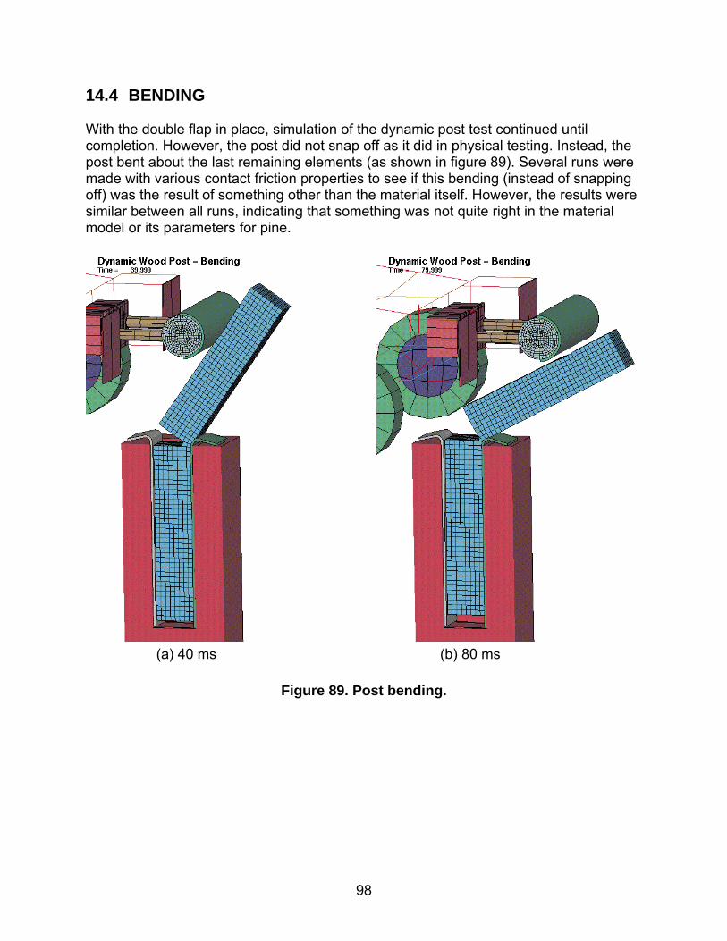
98

14.4 BENDING With the double flap in place, simulation of the dynamic post test continued until completion. However, the post did not snap off as it did in physical testing. Instead, the post bent about the last remaining elements (as shown in figure 89). Several runs were made with various contact friction properties to see if this bending (instead of snapping off) was the result of something other than the material itself. However, the results were similar between all runs, indicating that something was not quite right in the material model or its parameters for pine.

(a) 40 ms (b) 80 ms

Figure 89. Post bending.

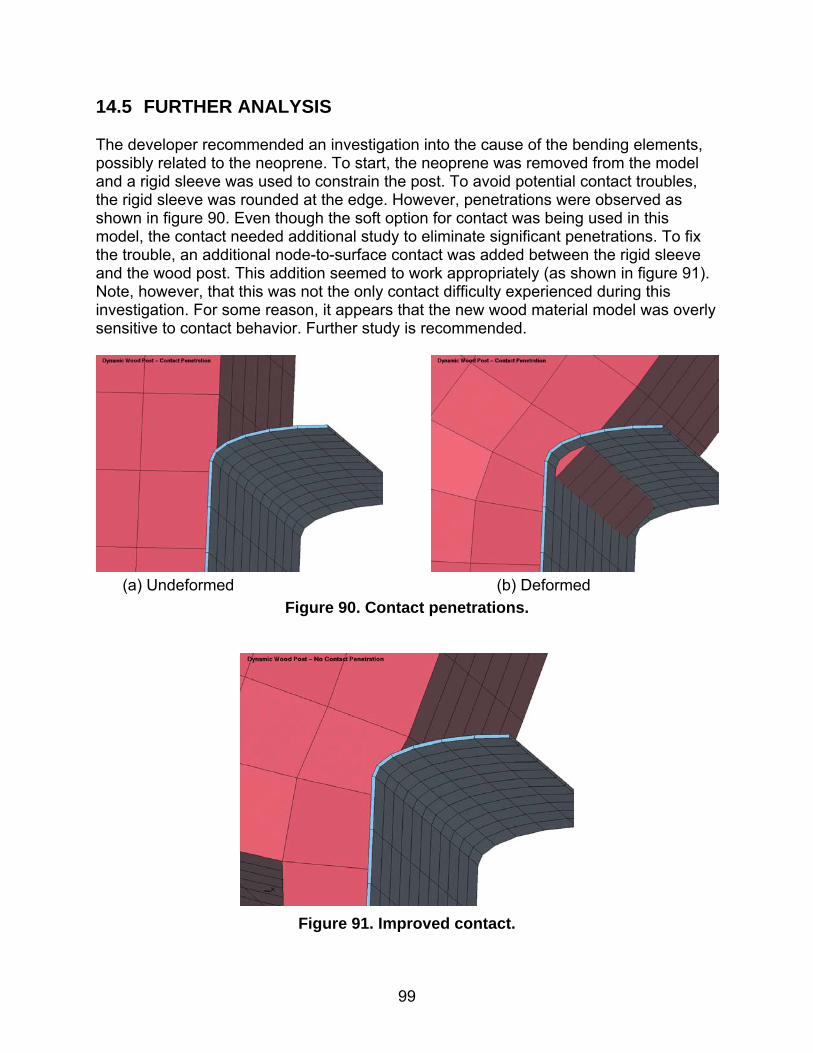
99

14.5 FURTHER ANALYSIS The developer recommended an investigation into the cause of the bending elements, possibly related to the neoprene. To start, the neoprene was removed from the model and a rigid sleeve was used to constrain the post. To avoid potential contact troubles, the rigid sleeve was rounded at the edge. However, penetrations were observed as shown in figure 90. Even though the soft option for contact was being used in this model, the contact needed additional study to eliminate significant penetrations. To fix the trouble, an additional node-to-surface contact was added between the rigid sleeve and the wood post. This addition seemed to work appropriately (as shown in figure 91). Note, however, that this was not the only contact difficulty experienced during this investigation. For some reason, it appears that the new wood material model was overly sensitive to contact behavior. Further study is recommended. (a) Undeformed (b) Deformed

Figure 90. Contact penetrations.

Figure 91. Improved contact.

100

With this latest model (i.e., rigid sleeve with no observable contact penetrations), the results were undesirable. Specifically, even with the previously discussed smaller time step of 0.001 ms being used, the lower post began to vaporize (as shown in figure 92). Also, the volume of the elements at the bottom of the post began to significantly expand (as shown in figure 93). This was discussed previously for a single-element model and it was noted that the user did not believe that this volume expansion was realistic.

(a) State 1 (b) State 2 (c) State 3 (d) State 4

Figure 92. Element vaporization at bottom of post. Figure 93. Volume expansion of 75 percent in an element near the bottom of post.

[ms] Time [ms]

Volu

me

(E+3

) [m

m3 ]

101

Next, because vaporization had returned to the model, it was thought that the cause might be a result of the time step (as discussed in section 6.2). However, when the time step was reduced again to 0.0005 ms and then even further down to 0.0001 ms, the results did not improve. In fact, using the very impractical time step of 0.0001 ms, vaporization occurred much more quickly in the model and caused the model to become unstable much earlier than with the larger time step. The deformed geometry of the post just before becoming unstable is shown in figure 94.

Figure 94. Vaporization with a time step of 0.0001 ms.

102

In a final attempt to determine more about the difficulties occurring with the dynamic post model (i.e., contacts, vaporization, bending instead of snapping off, etc.), the rigid-sleeve model with some contact penetrations (which alleviated the vaporization) was investigated near the damage area. It was believed that the failure of the wood elements away from the contact area would be unaffected by the contact penetrations. Unfortunately, the damaged area appeared to be incorrect (as shown in figure 95) (i.e., the elements in the center of the damage area became highly distorted, but did not erode). Plotting the damage of one of those elements showed that the element should have eroded since it had reached the critical value of 0.99 (the preset damage level for erosion) (see figure 96). (a) State 1 (b) State 2 (c) State 3

Figure 95. Highly distorted elements sometimes do not erode.

Figure 96. Damage of highly distorted element.

103

15 ELEMENT FORMULATION: HOURGLASSING There are three applicable solid-element formulations available within LS-DYNA:

1. Constant stress. 2. Fully integrated S/R solid. 3. Fully integrated quadratic eight-node element with nodal rotations.

These are listed in the order of increasing accuracy and in the order of increasing computational costs. Element formulation 1 can exhibit hourglassing, while formulations 2 and 3 have no hourglassing. The details for hourglassing and the various hourglass control algorithms will not be provided here. Readers are referred to the LS-DYNA user’s and theoretical manuals for details. Current simulation practices often use all three element formulations in a typical application where the post is considered to be critical for detailed modeling. A post is divided into three parts: (1) the area of loading, (2) the area around the ground line (breakage area), and (3) the remaining sections. Reasonable results have been obtained using element formulation 2 for the area of loading, formulation 3 for the ground line area, and formulation 1 for the rest of the post. An important goal of the new wood material model is too eliminate this cumbersome task of dividing a wood post into multiple parts. When using element formulation 1, an hourglass control algorithm is mandatory. The default hourglass control is referred to as control type 1. An important parameter associated with hourglass control is called the hourglass coefficient and is given the label qm. The default value is qm = 0.1. The new wood material model has exhibited hourglassing when element formulation 1 was used for the entire wood post. To quantify this phenomenon, the static wood post model was divided into three parts as described above. Hourglass energy and internal energy were compared for part 8002, which is the section of the post that breaks at ground level. Using default wood parameters for grade 1 southern yellow pine, hourglass control was investigated. The default hourglass control (type 1, qm = 0.1) results are shown in figure 97, while the results for hourglass control type 3 with qm = 0.1 are shown in figure 98. Clearly, both of these simulations resulted in excessive hourglassing (this is shown both graphically and numerically in the figures). When using hourglass control type 4 with qm = 0.005, the hourglass is brought under control for this model (as shown in figure 99). Note that hourglassing is considered to be under control when there are no obvious element distortions caused by hourglassing, and the hourglass energy measurement is less than 10 percent of the internal energy of the elements within a reasonable neighborhood of where the hourglassing is occurring.

104

Unfortunately, when using the same hourglass control that worked well for grade 1 southern yellow pine wood material properties for the grade DS-65 southern yellow pine wood material properties, significant hourglassing reappeared in the model (as shown in figure 100). Note that for chapters 13 and 14 of this report, hourglass control type 4 with qm = 0.005 was used throughout. (a) Deformed configuration (b) Hourglass energy

Figure 97. Southern yellow pine, grade 1: Hourglass control type 1, qm = 0.1. (a) Deformed configuration (b) Hourglass energy

Figure 98. Southern yellow pine, grade 1: Hourglass control type 3, qm = 0.1.

[ms] Time [ms]

[ms] Time [ms]

105

(a) Deformed configuration (b) Hourglass energy

Figure 99. Southern yellow pine, grade 1: Hourglass control type 4, qm = 0.005. (a) Deformed configuration (b) Hourglass energy

Figure 100. Southern yellow pine grade, DS-65: Hourglass control type 4, qm = 0.005.

To eliminate hourglassing completely and to increase the accuracy of the simulation, element formulations 2 and 3 were tried. Unfortunately, the results were undesirable because of the way failure (i.e., eroding) was handled for elements with multiple integration points. Thus, the developer has recommended that fully integrated element formulations not be used for the wood material. However, the user believes that fully integrated element formulations for the wood material model are critical for the success of the current implementation of the new wood material model. This would reduce the trial-and-error approach for finding the appropriate hourglass control parameters.

[ms] Time [ms]

[ms] Time [ms]

107

16 USER’S CONCLUSIONS Conclusions that were documented by the user and based on the validation effort detailed in chapters 8 through 15 of this report are as follows: Single-element models pulled in tension parallel to the grain behaved well and a parametric study involving grade, moisture content, and temperature yielded good results. Because of time limitations, various other single-element simulations were not performed, but are recommended (including compression, shear, and torsion loading both parallel and perpendicular to the grain). Static post test simulation results did not match the physical test results. The initial fracture strength of the simulation was good; however, the strength of the fracturing post was significantly below the minimum strength seen in physical testing. Wood material behavior is very sensitive to mesh size. When a refined mesh was used in the static post test simulation, the initial fracture strength was similar to the baseline model. However, the strength of the fracturing post dropped by almost an order of magnitude relative to the baseline model. The dynamic post test simulations had significant problems with time-step calculations, contacts, and bending behavior as opposed to a snap-off behavior. Further analysis resulted in post vaporization even when using an extremely small time step (0.0001 ms). Also, a significant volume expansion of the wood elements was noted (up to 75 percent volume expansion in individual elements). Additionally, highly distorted elements with damage values of 0.99 did not erode as expected. Because of these difficulties with the dynamic post simulations, a comparison to physical testing of dynamic posts was not made. Finally, hourglassing in the wood material model appears to be a very significant issue. A parameter study was needed to determine a good hourglass control type and hourglass control parameter for the dynamic post model. When the grade of the wood was changed from grade 1 to grade DS-65, hourglassing reappeared in the model using that same hourglass control. Fully integrated elements are not an option at this time because the eroding characteristics of the wood model do not behave well for fully integrated elements.

109

17 DEVELOPER’S COMMENTS ON USER’S EVALUATION This section was written by the developer and begins with topics selected by the developer and previously discussed by the user in chapters 9 through 16. These are topics that the developer concluded were worthy of additional discussion and explanation. These topics and the corresponding developer’s comments are briefly tabulated in table 7. Following this table is a more indepth discussion of these topics. For ease of discussion, each topic can be grouped roughly into one of three categories:

1. LS-DYNA code behavior. 2. User’s (analyst’s) responsibility. 3. Wood model theory or wood model input parameter selection.

Material models, like the wood and soil models, are not stand-alone codes. They are subroutines that work only in conjunction with the LS-DYNA code. Therefore, the results of any analyses performed depend on the formulation of the LS-DYNA code, the user’s specification of the geometric mesh and boundary conditions, the user’s specification of the input parameter values for various LS-DYNA features and material models, and the formulation and input parameter values for the wood material model. The user’s evaluation chapters demonstrate the behavior of the finite element systems under various operating conditions. By system, we mean the wood material model used in conjunction with other material models/structures and LS-DYNA controls. An example is a vehicle impacting a wood post embedded in a neoprene and concrete support structure. Code issues are related to the functioning of the LS-DYNA features via the LS-DYNA controls, which affect the behavior of the system. These controls are independent of the wood model and are typically proprietary in formulation. The user’s issues are related to the proper user’s setup of the finite element mesh, the user’s regard for LS-DYNA diagnostics, and the user’s selection of LS-DYNA input parameters. It is the user’s responsibility to learn the LS-DYNA code, set up the mesh properly, and input the correct control parameters. Most calculations documented by the user show good system behavior, with the wood material model behaving realistically. However, some calculations show poor system behavior, which the user did not adequately explain. The user is a potential end user of the code (not a material model or code developer) and, therefore, did not distinguish between LS-DYNA code issues, user’s setup and input parameter selection issues, and wood model issues. Of the 10 topics chosen for discussion, we can categorize 5 as code- and user-related issues, and 5 as wood model issues. No changes to the wood model theory or wood model input parameter values affect the results regarding the five code- and user-related issues. The five wood model issues are:

• Volume expansion and contraction. • Static post simulation behavior.

110

• Mesh-size dependency. • Post breakage and fracture. • Erosion criteria.

The developer performed many additional calculations that were related to some of these wood model issues, as discussed in section 17.3. The additional calculations indicate that none of the wood model issues are wood model deficiencies that warrant changes to the theoretical formulation of the model. However, changes to the wood model input parameter values may positively affect the results.

The developer wishes to thank the user for providing a detailed report on the initial use of the wood material model. The questions and comments provided by a novice user of the wood model are a good learning tool for other novice users. However, the tone and conclusions (or lack thereof) in some portions of the user’s evaluation report in chapters 9 through 16 may leave the reader wondering whether the wood model is ready for use. Both the developer’s and the user’s wood model evaluation sections were reviewed by individuals at FHWA, NHTSA NCAC, and each COE before publication. One experienced analyst and reviewer stated that he understood that many of the issues brought up by the user were LS-DYNA code and user input parameter selection issues, and not wood model issues. However, a beginning analyst might not make this distinction and think that the model was deficient. This is because the user’s evaluation report brings up various issues without thoroughly defining them or resolving them and, more importantly, without identifying how the issue relates to the wood material model. Therefore, all analytical results provided by the user have been included in this report, whether or not the simulation was performed correctly, and whether or not the problem and solution are directly related to the wood model. As the developer, we believe that this consolidated, comprehensive report provides a very valuable learning tool for analysts who want to learn how to use the wood (or soil) model as part of the LS-DYNA code. We think that identifying and providing commentary on issues is a much better approach than removing issues that are not directly related to the wood model. Some of the issues in the user’s evaluation report are potential hurdles that other users may run into and, therefore, warrant publication. We hope that the following discussion provides inexperienced users with guidelines on how to correctly run the wood model. It is the developer’s opinion that the user’s wood model evaluation revealed no substantial problems with the model. In fact, the developer performed various analyses to positively determine that none of the issues were model deficiencies. The developer has demonstrated that all of the user’s evaluation calculations gave reasonable results when reasonable LS-DYNA control parameters and reasonable wood input parameters were used. In particular, see section 17.3 for a thorough discussion of the excessive erosion problem and solution, and a discussion of post breakage.

17.1 TABLE OF WOOD MODEL TOPICS Table 11. Developer’s response to user’s review of wood model.

Developer’s Response Issue User’s Comment Wood

Model Problem?

Adjust Wood Input?

Volume Expansion and Contraction

Wood is incompressible, while wood material model admits compressible behavior.

- FPL data show compressibility of wood. - User does not furnish incompressible data.

No No

Static Post Simulations

Calculated forces fall below minimum seen during tests.

- Developer’s calculations show excellent correlation with data.

No No

Mesh-Size Dependency

Wood model behavior is very sensitive to mesh size.

- Wood softening model is formulated to be mesh-size independent; verified on single elements. - User has not demonstrated that mesh-size dependency is related to the wood model. - Geometric or contact portion of the model is suspect.

Probably not

No

Time-Step Control Time-step reduction is needed to prevent excessive erosion of wood model.

- LS-DYNA diagnostics indicate that stable time step was exceeded because of user’s input specification. - Calculations remain stable with stable time step.

No No

Post Breakage and Fracture

Post bends rather than snapping off. - Developer’s calculations demonstrate snap-off behavior. - Adjustment of input parameters/boundary conditions affects snap-off behavior. - Default parameters could be adjusted if snap-off time is furnished by testers.

No Yes

Element Erosion Excessive erosion of elements occurs where post contacts support.

- LS-DYNA diagnostics indicate substantial initial penetration, which is a result of the user’s input. - User should redefine mesh and contact.

No No

Erosion Criteria Elements should erode when damage reaches 99 percent.

- Not true - Elements erode when all six stress components reach 99 percent damage.

No No

111

Table 11. Developer’s response to user’s review of wood model (continued). Developer’s Response

Issue User’s Comment Wood Model Problem?

Adjust Wood Input?

Hourglassing Hourglassing of the wood model appears to be a very significant issue.

- Hourglassing occurs for ALL material models with under-integrated elements. - Developer demonstrates significant hourglassing for elastic material model 1. - Hourglass controls are separate from wood model.

No No

Fully Integrated Elements

Fully integrated elements are not an option at this time.

- Disagree - Developer demonstrates excellent results with fully integrated elements while exercising caution on erosion.

No No

Contact Surfaces Wood model is overly sensitive to contact surfaces.

- Disagree - Surface penetration controlled by contact algorithms, not the material model. - Developer demonstrated similar penetration with elastic material model 1.

No No

112

113

17.2 DISCUSSION OF WOOD MODEL TOPICS These items are listed in the order that they were brought up by the user in chapters 9 through 16. Volume Expansion and Contraction: The user demonstrates that the volume of the single elements pulled in tension expands by as much as 6 percent (previously shown in figure 73). The user believes that there should be no change in volume for wood (i.e., wood is incompressible, but shows no credible data or peer-reviewed documentation to support this position). It is the developer’s position that Poisson’s ratios measured by FPL and reported in the literature(11) do not support the assumption of incompressibility. Therefore, modeling wood as an incompressible material is not recommended by the developer. The suite of clear wood data provided by FPL (documented in the user’s manual)(2) included measurement of the major Poisson’s ratio in the elastic region. A transversely isotropic material such as wood has three ratios. Typical values are around νLT = 0.16, νTL = 0.004, and νTR = 0.4 for pine at the fiber saturation point. No measurements were reported for the effective Poisson’s ratios in the plastic/damage regions (once the material yields or softens). By effective Poisson’s ratio, we mean the ratio of the lateral strain to the axial strain in uniaxial stress tests (without lateral confinement). Porous materials tend to flow during yielding and softening, which can result in an effective Poisson’s ratio that is larger or smaller than the elastically measured value. For example, for porous geological materials such as concrete, the effective Poisson’s ratio is typically modeled as greater than the elastic ratio in unconfined compression (with values greater than 1) and less than the elastic ratio in unconfined tension. The effective ratio depends on the shape of the yield surfaces, coupling of the yield surfaces, and how the plasticity algorithm is formulated. To achieve no change in volume, the elastic and effective Poisson’s ratios would have to be 0.5. The FPL data indicate that the elastic Poisson’s ratios are not 0.5. However, no lateral strain or change in the volume measurements is available to confirm or refute an effective Poisson’s ratio of 0.5 in the plastic region. Therefore, we recommend that any future test data generated (such as uniaxial tension and compression tests) include lateral strain measurements. For a material to be modeled as incompressible in the elastic region, it must also be modeled as isotropic. By examining the elastic constitutive equations in the wood model user’s manual,(2) one can readily determine that all Poisson’s ratios can only be equal to 0.5 when all stiffnesses (parallel and perpendicular) are equal. Wood, on the other hand, is modeled as transversely isotropic (a simplification of orthotropic) because the stiffness parallel to the grain is about 50 times greater than that perpendicular to the grain. Another point to note is that the volume change being modeled implicitly includes expansion and compaction of pores and the opening up of fracture surfaces. This is

114

demonstrated schematically in figure 101. The formation of voids and the compaction of pores are shown in figure 102. The fracture of wood creates voids, which are modeled as volume expansion with continuum models like the wood model. Wood is also porous. The crushing of pores is modeled as volume compaction.

(a) Fracture of wood (specimen breaks in two) (b) Finite element simulation (element stretches) Figure 101. Schematic demonstration of how a finite element treats fracture prior

to erosion.

(a) Void formation(11) (b) Pore compaction(11) Figure 102. Demonstration of void formation and crushing of wood specimens.

115

Setting the compressibility or effective Poisson’s ratio behavior of the wood model is not simply a matter of specifying an input value. Rather, it requires changes to the formulation of the model to include coupling between the parallel (axial) plasticity and perpendicular (lateral) plasticity. The current wood model includes separate yield surfaces and plasticity computations for yielding parallel and perpendicular to the grain. As a result, yielding parallel to the grain does not induce plastic flow perpendicular to the grain. Similarly, yielding perpendicular to the grain does not include plastic flow parallel to the grain. We recommend exploring and implementing methods of coupling the plastic flow once sufficient test data are generated to set the coupling via measurement of the effective Poisson’s ratio or volume change. Static Post Simulations: The user states that, during fracture, the wood model is too weak: Once the post begins to fail, the simulation forces fall below the minimum force levels seen in testing. As the developer, we disagree. Comparison of the simulation force histories with data (as opposed to performance envelopes) demonstrates that the simulation forces are not too low. In addition, excellent correlations between the simulations and the performance envelopes are achieved through careful selection of the input fracture energy. No changes to the material model formulation are required to achieve good agreement between the simulations and the static post test data. We suggest that the user plot all data curves in comparison to the performance envelopes and more thoroughly discuss their performance envelope selection process. The static data are highly scattered and display both brittle and ductile behaviors.

Figure 103. User’s grades 1 and 1D simulation compared to the performance envelopes, using Gf|| = 50 Gf⊥.

116

(a) Set 1 (b) Set 2

Figure 104. Most of the grades 1 and 1D static post test measurements exhibit

brittle behavior.

The user’s simulation and performance envelopes are shown in figure 103. The suite of test data used to generate these performance envelopes is shown in figure 104 for grades 1 and 1D. The simulation conducted by the user peaks at about 47 MPa, then softens in a brittle mode between 25 and 50 mm of deflection. The behavior of the simulation is similar to 9 out of 15 of the data curves shown in figure 104, which fail in a brittle mode between 25 and 50 mm of deflection. This is good agreement. However, it is evident that the user’s simulation fails in a more brittle manner than that represented by the performance envelopes. The user supposedly constructed the envelopes using curves from posts that exhibited the most typical behavior. The minimum and maximum curves, which define the performance envelopes, do not represent any one particular curve from the tests. The simulation was conducted using the default fracture energies recommended by the developer. Good agreement between the simulation and the performance envelopes can be achieved by increasing the parallel-to-the-grain fracture energy above the default value (as shown in figure 105). Refer to chapter 5 for a thorough review of the developer’s static post simulations. Simulations conducted at two different fracture energies were previously shown in figure 22. The calculation with Gf

|| = 50 Gf ⊥ (green dotted line)

agrees with the brittle data. The calculation with Gf || = 250 Gf ⊥ (red solid line) agrees with the ductile data. It is important to note that the default fracture energy for saturated room-temperature pine is based on correlations with the dynamic (bogie impact) performance envelopes. A higher value than the default is needed to achieve good correlations with the static performance envelopes.

(mm) 0 51 102 152 203 254

(mm) 0 51 102 152 203 254

Brittle

Ductile

90 45 0

90 45 0

Forc

e (k

N)

Forc

e (k

N) Ductile

Brittle

117

Figure 105. Good correlation is achieved between the simulation and the

performance envelopes by increasing the fracture energy above the default value (to Gf|| = 250 Gf⊥).

Mesh-Size Dependency: The user suggests that the wood model is mesh-size dependent because static post calculations conducted at two different mesh refinements (25.4-mm and 12.7-mm elements) exhibit different late-time force-deflection behaviors. These behaviors were previously shown in figure 78. It is not clear to the developer that the origin of the different late-time responses is the wood model, rather than the overall (geometric/material/contact) model. The user demonstrated mesh-size sensitivity of a finite element system. However, the user did not demonstrate that the sensitivity was a result of the wood model formulation. The origin of the different responses is an issue because the developer could possibly adjust the model formulation if the material model is the source of the different responses, otherwise, the geometric model must be adjusted. Often, material models exhibit mesh-size sensitivity because of their softening formulations. However, the developer included coding to regulate mesh-size sensitivity by making the softening formulation of the wood model a function of element size and checking this behavior for single elements. The softening formulation of the wood model for single elements does not depend on element size. In addition, the user’s early-time force-deflection behaviors are in good agreement for peak strength and initial softening, which suggests that the softening formulation has been adequately regulated. On the other hand, the developer’s static post calculations discussed in chapter 5 (for example, see figure 27) indicate that the late-time behavior is the most sensitive portion of the simulations. For example, the late-time behavior is sensitive to input parameter selection, hourglass control, element formulation, and geometric modeling details. In fact, two other reviewers suggested that the perceived mesh-size sensitivity is not an

118

issue because the discrepancy in the response occurs at a late time, where data are not adequately measured. We note that the deformed configurations in the user’s plots look different in the region where the post is rolling over the rounded edge on the brace. It appears that more wood compaction is taking place at this location in the crude mesh than in the refined mesh. Therefore, the source of the sensitivity could also be a result of modeling details in this region. We recommend reexamining this calculation in the future to determine the source of the mesh-size sensitivity. If the wood model is the source of the sensitivity, then modifications should be made to make the material model independent of the mesh size. Perhaps simpler geometries and loads, such as direct pull (with softening) and unconfined compression (with hardening) of coupons or timbers, could be used to evaluate the model’s mesh-size response. Unconfined compression is suggested so that the mesh-size sensitivity of the hardening formulation can be evaluated. In particular, single material simulations that isolate the wood model without the use of other materials, contact surfaces, and complex boundary conditions are recommended. Time-Step Control: The user reports that a reduction in the time step is needed to control excessive erosion of the wood model (instability), as previously shown in figure 87. The user corrected this behavior by reducing the time step via the *CONTROL_TIMESTEP command. The developer disagrees with this assessment because the user requested that the LS-DYNA code exceed the stable time for contact surface stability. Thus, the calculation became unstable. The instability is the result of a deliberate override of the stable time step for the contact surfaces, not the wood model, and is caused by the user's input. A review of the user’s input files and output diagnostics indicates that the time step for stable contact surface behavior was exceeded in the user’s calculations. This is because the user requested, via the *CONTROL_CONTACT card, that the stable time step for contact surface stability be ignored. In other words, the user first increased the time-step size above the stable value via *CONTROL_CONTACT (and caused an instability), then reduced the time-step size below the stable value via *CONTROL_TIMESTEP (to relieve the instability). This dual process is both unnecessary and inefficient. The developer recommends letting LS-DYNA automatically select the time-step size based on the element size, wave transit time, and contact surface stability. All calculations performed by the developer in chapters 1 through 9 remained stable because the developer did not override the stable LS-DYNA time step. A very thorough discussion of instabilities in the post-impact analyses is discussed in section 17.3. Post Breakage/Fracture: The user reports that the post is bending, rather than snapping off, and suggests that “something is not quite right in the material model or its parameters for pine.” The developer has demonstrated both snapping (complete

119

breakage) and bending (partial breakage) behaviors with the wood model. Five calculations that demonstrate complete breakage are:

1. Grade 1 pine with small adjustments in default quality factors (as previously shown in figure 43).

2. DS-65 post modeled with simple pinned boundary conditions (as shown in figure 106 below).

3. Grade 1 pine with post-peak hardening (as shown in figure 117 of section 17.3). 4. Grade 1 Douglas fir (as shown in figure 118 of section 17.3). 5. Grade 1 pine impacted at 29.5 m/s (66 miles per hour (mi/h)) (as shown in figure

119 of section 17.3).

(a) Without modeling rate effects (b) With modeling rate effects

Figure 106. DS-65 pine post modeled with simple pinned boundary conditions. No data was documented that indicated the snap-off time (average and scatter) that occurred in the bogie impact tests, so snap-off time was not used to set the default parameters. It is our understanding that the data for the breakage of wood posts are highly scattered. Post breakage does not occur at one particular time after impact or at a particular deflection. No theoretical model changes are required to simulate snap-off. This is an input parameter selection issue, not a wood model formulation issue. The default parameters could readily be adjusted to modify the snap-off time given the appropriate data. However, input parameter values are ultimately the responsibility of the user. To elaborate, calculations conducted using the final default properties for saturated room-temperature pine, reported by either the developer or the user, indicate that post breakage is incomplete at 180 mm, which is the final deflection of the performance envelope plots. However, a number of calculations performed by the developer

C

120

simulated complete breakage. For example, the developer determined that adjustments in the quality factors affect the deflection at which the post breaks in two. This was previously demonstrated in figure 43. Here, the default quality factors for grade 1 pine were adjusted from QT = 0.47 and QC = 0.63 to QT = 0.4 and QC = 0.7. This adjustment of the quality factors reduces the tensile strengths and increases the compressive strengths. Recall that the quality factors are applied to the clear wood strengths (QT to the tensile and shear strengths, and QC to the compressive strengths) to reduce the strength as a function of the grade. The trend noted is that the post will break earlier in time as QT is adjusted downward and QC is adjusted upward. The load-deflection and bogie velocity-reduction curves calculated with either set of quality factors are similar (refer back to figures 43 and 44). The snap-off time may also be dependent on other material properties besides strength. The developer suggests that each user examine:

• Rate effects: Rate effects tend to make the simulation more elastic, which should enhance standoff.

• Late-time hardening in compression via the Ghard parameter: This parameter was implemented to override perfect plasticity in compression.

• The parameter IQUAL: By default, the quality factors are simultaneously applied to both the parallel and perpendicular strengths. As an option, setting IQUAL to 1 removes the application of the quality factors from the perpendicular strengths. This would strengthen the behavior perpendicular to the grain.

The snap-off behavior not only depends on the behavior of the wood material model, but on the overall behavior of the geometric and material models in the snap-off region (neoprene, contact, and mesh refinement), and on how the wood post is being loaded and pulled (or not pulled). For example, the wood post is more likely to snap off with more pull (from higher tensile stresses). The amount of pull depends on how the post is gripped in the support and the contact between the bogie cylinder and the post. The post slides up the support in the simulations (perhaps a couple of inches or more). Also, the impact cylinder bounces off the post with little late-time contact in the simulations. The developer never received feedback from the user (testers) on how this simulated behavior compared to the measured behavior. Future efforts could further explore the material parameters and geometric issues that affect snap-off. However, the developer strongly recommends that each user evaluate the default material properties prior to their use. The developer has made its best effort to set the default parameters with the test data, time, and funding available for this project. However, users are not limited to using default properties and are encouraged to do their own evaluation and share their results with others in the roadside safety community.

121

Excessive Erosion at Bottom of Post: The user reports excessive erosion where the post is in contact with the rigid support (as previously shown in figure 85). The developer determined that this excessive erosion is not a problem in the wood model formulation. Rather, it is caused by user input. The user meshed the rigid support such that it penetrated the wood post, and this interpenetration caused the instability. The LS-DYNA code provided warning diagnostics to assist in determining the cause of the instability; however, these warnings were ignored by the user. This issue is thoroughly discussed in section 17.3 below. Damage: The user incorrectly states that elements should erode when damage reaches 99 percent. This is not true. Elements automatically erode when all six stress components reach 99 percent damage via the parallel damage parameter. The elements do not automatically erode when the three perpendicular stress components reach 99 percent damage via the perpendicular damage parameter. The wording in the wood model user’s manual(2) has been updated in an attempt to make this point clear. To elaborate, the user plotted the default damage and noted that some elements do not erode when the plotted damage reaches 99 percent. By default, the maximum of either the parallel or the perpendicular damage parameters is plotted. Therefore, the damage being plotted by default could be the parallel damage parameter or it could be the perpendicular damage parameter, whichever is larger. The elements automatically erode when the parallel damage parameter exceeds 99 percent, but not when the perpendicular damage parameter reaches 99 percent (unless IFAIL = 1, as set by the user). Therefore, damage that is 99 percent, but not accompanied by erosion, is perpendicular damage. Alternatively, the user may request that only perpendicular damage be plotted by setting NPLOT = 2. Hourglassing: The user states that hourglassing appears to be a very significant issue for the wood model. The developer states that hourglassing occurs when under-integrated elements are used with any material model, not just the wood model. For example, even a simple elastic material model generates as much hourglass energy as the wood model in the static post simulation shown in figure 107. The developer discusses hourglass control in section 5.3. Hourglass controls are separate from the material models. Fully Integrated Elements: The user erroneously states that fully integrated elements are not an option for the wood model at this time. This is not true. The developer obtained excellent results with fully integrated elements (as previously shown in figure 27). Our only caution is that users must recognize that fully integrated elements erode when any one of the eight integration points fails, regardless of which material model is used.

122

Wood Material Model

(a) Deformed configuration for wood model (b) Energy ratio Elastic Material Model

(c) Deformed configuration (d) Energy ratio for elastic material model

Figure 107. Developer’s static post simulations using hourglass stiffness

type 4 with a reduced (0.03) coefficient.

C

0

.00

5

.00

1

0.00

1

5.00

2

0.00

2

5.00

3

0.00

3

5.00

4

0.00

4

5.00

5

0.00

5

5.00

6

0.00

6

5.00

7

0.00

7

5.00

8

0.00

8

5.00

9

0.00

9

5.00

10

0.00

0.00E+00

2.00E-02

4.00E-02

6.00E-02

8.00E-02

1.00E-01

1.20E-01

1.40E-01

1.60E-01

1.80E-01

2.00E-01

2.20E-01

2.40E-01

2.60E-01

2.80E-01

3.00E-01 MWRSF BENDING TEST SIMULATION CLEAR WOOD PINE SATURATED

Mat

eria

l Hou

rgla

ss /I

nter

nal E

nerg

y R

atio

Time minimum = 0.0000E+00 maximum = 3.0030E-01

Material A=1, B=2, C=3, D=4, E=5,

A

A

AA A

A

A

BB B

B BC

C

C

C

C

C

D

DD

D

D

D

E

EE

E

E

Loaded Region – 30%

Break Region – 14%

Hou

rgla

ss-to

-Inte

rnal

En

ergy

R

atio

(%

)

28

24

20

16

12

8

4

0

Time [ms]

Loaded Region

Break Region

Hou

rgla

ss-to

-Inte

rnal

Ene

rgy

Rat

io (%

)

123

Contact Surfaces: The user misleadingly states that “for some reason, the wood model is overly sensitive to contact surfaces,” after noting penetration between the wood post and the liner previously shown in figures 68 and 91. Contact surface penetration is controlled by the user’s selection of the contact type and the input, not by the material model formulation or input. This is not a wood model issue that requires changes to the wood model formulation or wood model input parameters. See section 17.3 for a discussion of the penetration problem. It has been demonstrated that similar penetration behavior is simulated with an elastic post (Mat 1) as with a wood post (Mat 143). It has also been demonstrated that penetration was relieved using a different version of the code. A user should realize that contact algorithms use material stiffness to relieve penetration. The stiffness extracted from orthotropic materials such as wood is the greatest stiffness. For saturated wood, the greatest stiffness is parallel to the grain and is 50 times greater than the stiffness perpendicular to the grain. The user should note whether the contact is parallel or perpendicular to the grain and should adjust contact surface parameters accordingly.

17.3 INSTABILITIES IN DYNAMIC ANALYSES The user’s LS-DYNA simulations of wood posts impacted by bogie vehicles sporadically behave in an unstable manner (for example, see chapter 14). The objective of this section is to help the reader understand the conditions that lead to this unstable behavior. This is accomplished by running the user’s exact LS-DYNA input file on the developer’s computer system, then determining which input parameters cause the instability. Unless otherwise specified, the developer’s calculations are conducted with beta version 970, revision 1877 (Intel-based PC). The user’s calculations are conducted with beta version 970, revision 1812 (SGI Octane). Demonstration of Unstable Behavior Two calculations were conducted by the developer to demonstrate unstable behavior. The mesh used in each calculation is nearly identical (both created by the user). The main difference between the two calculations is the inclusion of a second flap of neoprene between the post and the concrete support (as shown in figure 108). The other differences are in the input:

• Rate effects (turned on in the single-flap analysis, turned off in the double-flap analysis).

• Initial velocity specification (not applied to the cylinder neoprene in the single-flap calculation, but applied to the cylinder neoprene in the double-flap calculation).

• Output force plane location (76 mm (3 inches) below the impact location in the single-flap calculation, 51 mm (2 inches) below the impact location in the double-flap calculation).

124

(a) Single flap (b) Double flap

Figure 108. Finite element meshes used in demonstration problems. Mesh With Single Flap: This calculation did not exhibit unstable behavior on the developer’s computer system. The deformed configurations at the various time steps are shown in figure 109. Mesh With Double Flap: This calculation exhibited unstable behavior. The unstable behavior was sudden excessive erosion of the wood post, primarily between the impact and breakaway regions. Excessive erosion is shown in figure 110. LS-DYNA diagnostics indicate that numerous elements are being deleted with negative volume.

Flap No Flap

Flap Flap

125

(a) 0.0 ms (b) 30 ms (c) 50 ms (d) 100 ms Figure 109. Stable behavior in the developer’s single-flap calculation.

(a) 0.0 ms (b) 10.752 ms (c) 10.785 ms (d) 11.0 ms

Figure 110. Unstable behavior in the developer’s double-flap calculation. These calculations indicated that small changes in the mesh and input can trigger instabilities. Variation of Instabilities by Computer Platform The developer’s calculations with the single and double flaps were conducted on an Intel-based PC (using Windows) computer platform. These same calculations were

126

conducted by the user on their SGI Octane (using UNIX) computer platform. The user’s results also demonstrated excessive erosion; however, they were not identical to the developer’s results. The main difference was that the user noted unstable behavior in both calculations (single and double flap), whereas the developer only noted unstable behavior in one calculation (double flap). The unstable behavior in the user’s single-flap calculation is shown in figure 111.

127

(a) 0.0 ms (b) 10.501 ms (c) 10.750 ms (d) 10.801 ms

Figure 111. Unstable behavior in the user’s single-flap calculation.

These comparisons indicated that the unstable behavior was not identical and reproducible from computer platform to computer platform. Time-Step Control The diagnostics provided by the LS-DYNA code indicated that a possible source of the instability was the time step (because of the contact surface algorithms). The output diagnostics from both the single- and double-flap analyses are shown in figure 112. This output indicates that the stable time step for the contact surface algorithms is less than that calculated for the critical element (which is based on the element size and the wave transit time across the element).

128

(a) Single flap

(b) Double flap

Figure 112. LS-DYNA MESSAG file which shows that the stable time step is

exceeded. A review of the LS-DYNA input file provided by the user indicates that the user specified that contact stability be ignored for the time-step determination (via the eroding contact time step parameter (ECDT) on the *CONTROL_CONTACT). Therefore, two calculations were conducted by the developer to determine whether the instabilities were relieved when contact stability was considered for the time-step determination:

The LS-DYNA time step size should not exceed 0.235E-02 to avoid contact instabilities. If the step size is bigger then scale the penalty of the offending surface. 0 t 0.0000E+00 dt 0.00E+00 flush i/o buffers 1 t 0.0000E+00 dt 5.01E-03 flush i/o buffers 1 t 0.0000E+00 dt 5.01E-03 write d3plot file 1118 t 5.0000E+00 dt 4.36E-03 write d3plot file 2279 t 9.9985E+00 dt 4.25E-03 write d3plot file 3498 t 1.4998E+01 dt 3.99E-03 write d3plot file 4769 t 1.9997E+01 dt 3.83E-03 write d3plot file 5000 t 2.0874E+01 dt 3.76E-03 flush i/o buffers 6143 t 2.4999E+01 dt 3.62E-03 write d3plot file 7603 t 3.0000E+01 dt 3.33E-03 write d3plot file 7603 t 3.0003E+01 dt 3.33E-03 write d3dump01 file

The LS-DYNA time step size should not exceed 0.235E-02 to avoid contact instabilities. If the step size is bigger then scale the penalty of the offending surface. 0 t 0.0000E+00 dt 0.00E+00 flush i/o buffers 1 t 0.0000E+00 dt 5.01E-03 flush i/o buffers 1 t 0.0000E+00 dt 5.01E-03 write d3plot file 205 t 9.9578E-01 dt 4.53E-03 write d3plot file 448 t 1.9972E+00 dt 3.88E-03 write d3plot file 693 t 2.9998E+00 dt 4.31E-03 write d3plot file 922 t 3.9962E+00 dt 4.26E-03 write d3plot file 1156 t 4.9982E+00 dt 4.20E-03 write d3plot file 1392 t 5.9970E+00 dt 4.20E-03 write d3plot file 1635 t 7.0000E+00 dt 4.07E-03 write d3plot file 1874 t 7.9981E+00 dt 4.39E-03 write d3plot file 2112 t 8.9964E+00 dt 4.18E-03 write d3plot file 2350 t 9.9974E+00 dt 4.19E-03 write d3plot file

129

1. Time Step Set Considering Contact Stability: The *CONTROL_CONTACT card allows the user to specify whether or not contact stability is considered by LS-DYNA when determining the time step of each calculation. By default, contact stability is considered with LS-DYNA, version 970 (at least for the *CONTACT_ERODING_SINGLE_SURFACE algorithm used in these calculations). The double-flap calculation conducted by the developer is stable if the time step is based on the minimum needed for contact stability via the default value of ECDT on the *CONTROL_CONTACT card. The deformed configuration at 30 ms is shown in figure 113. LS-DYNA diagnostics are shown in figure 114(a).

2. Time Step Set Globally: Another option is to scale back the element-based time

step via the *CONTROL_TIMESTEP card. The double-flap calculation conducted by the developer is stable if the time step is scaled back to 40 percent of the element-based step. This reduces the initial time step to that needed for stable contact behavior. The results are identical to those shown in figure 113. LS-DYNA diagnostics are shown in figure 114(b). Keep in mind that for this calculation, the time step was scaled up by overriding the time step for stable contact via *CONTROL_CONTACT, then scaled down via *CONTROL_ TIMESTEP. This is the way that the user ran their calculations to control stability.

(a) 0.0 ms (b) 15 ms (c) 50 ms (d) 100 ms

Figure 113. Stable behavior is achieved by reducing the time step to that needed

for stable contact surface behavior (default grade 1 saturated pine properties without rate effects).

130

(a) *CONTROL_CONTACT

(b) *CONTROL_TIMESTEP Figure 114. LS-DYNA MESSAG file with diagnostics for the stable time step.

The LS-DYNA time step size should not exceed 0.235E-02 to avoid contact instabilities. If the step size is bigger then scale the penalty of the offending surface. 0 t 0.0000E+00 dt 0.00E+00 flush i/o buffers 1 t 0.0000E+00 dt 2.23E-03 flush i/o buffers 1 t 0.0000E+00 dt 2.23E-03 write d3plot file 2606 t 4.9993E+00 dt 1.85E-03 write d3plot file 5000 t 9.3315E+00 dt 1.81E-03 flush i/o buffers 5367 t 9.9986E+00 dt 1.81E-03 write d3plot file 8161 t 1.4998E+01 dt 1.81E-03 write d3plot file 10000 t 1.8351E+01 dt 1.80E-03 flush i/o buffers 10936 t 1.9999E+01 dt 1.74E-03 write d3plot file 13868 t 2.4999E+01 dt 1.63E-03 write d3plot file 15000 t 2.6814E+01 dt 1.58E-03 flush i/o buffers 17062 t 2.9999E+01 dt 1.51E-03 write d3plot file 20000 t 3.4343E+01 dt 1.45E-03 flush i/o buffers 20455 t 3.5000E+01 dt 1.44E-03 write d3plot file 23978 t 4.0000E+01 dt 1.41E-03 write d3plot file 25000 t 4.1440E+01 dt 1.47E-03 flush i/o buffers 27565 t 4.4999E+01 dt 1.38E-03 write d3plot file 30000 t 4.8342E+01 dt 1.37E-03 flush i/o buffers 31210 t 5.0000E+01 dt 1.37E-03 write d3plot file 31210 t 5.0001E+01 dt 1.37E-03 write d3dump01 file

The LS-DYNA time step size should not exceed 0.235E-02 to avoid contact instabilities. If the step size is bigger then scale the penalty of the offending surface. 0 t 0.0000E+00 dt 0.00E+00 flush i/o buffers 1 t 0.0000E+00 dt 2.11E-03 flush i/o buffers 1 t 0.0000E+00 dt 2.11E-03 write d3plot file 2365 t 4.9983E+00 dt 2.11E-03 write d3plot file 4730 t 9.9986E+00 dt 2.11E-03 write d3plot file 5000 t 1.0570E+01 dt 2.11E-03 flush i/o buffers 7095 t 1.4999E+01 dt 2.11E-03 write d3plot file 9460 t 1.9999E+01 dt 2.11E-03 write d3plot file 10000 t 2.1141E+01 dt 2.11E-03 flush i/o buffers 11825 t 2.5000E+01 dt 2.11E-03 write d3plot file 14189 t 2.9998E+01 dt 2.11E-03 write d3plot file 15000 t 3.1713E+01 dt 2.11E-03 flush i/o buffers 16554 t 3.4998E+01 dt 2.11E-03 write d3plot file 18919 t 3.9999E+01 dt 2.11E-03 write d3plot file 20000 t 4.2284E+01 dt 2.11E-03 flush i/o buffers 21284 t 4.4999E+01 dt 2.11E-03 write d3plot file 23649 t 5.0000E+01 dt 2.11E-03 write d3plot file 23649 t 5.0002E+01 dt 2.11E-03 write d3dump01 file

131

The user conducted their single- and double-flap calculations by reducing the time step via the *CONTROL_TIMESTEP method. Stable behavior was achieved in both their single- and double-flap calculations (consistent with the developer’s results).

Based on these example calculations, the option recommended by the developer is to let LS-DYNA, by default, automatically calculate and use the stable time step. This means leaving ECDT as zero on the *CONTROL_CONTACT card. The default *CONTROL_CONTACT method selects the optimal time step throughout the run time of the calculation. On the other hand, with the *CONTROL_TIMESTEP option, the user must review the run-time diagnostics, then stop and rerun the calculation with a reduced time step. Runs Conducted With Different Contact Surface Types The developer conducted both the single- and double-flap calculations with different contact surface formulations to further search for instabilities. LS-DYNA has 25 contact surface types. Four types were examined here: Eroding Single Surface: All calculations discussed in the previous paragraphs used this formulation. Instabilities, if they occurred, appeared as eroding wood post elements. The input specified seven parts to this contact surface (the neoprene on the impact cylinder, the three parts of the wood post, the two neoprene liners on each side of the post, and the rigid-concrete support). Single Surface: One double-flap calculation was conducted with this formulation. The calculation terminated early (at 2.9 ms) because of the negative volume of an element within the neoprene liner. The offending element is shown in figure 115. The liner is modeled as an elastic material. This calculation demonstrates that contact surface instabilities affect different parts of the mesh. The instability was not eliminated by reducing the time step below that needed for contact surface stability. The developer also checked the *CONTACT_SINGLE_SURFACE performance using an older version of LS-DYNA (beta version 970, revision 1553). The calculation did not run past the initialization stage. Instead, the calculation terminated at time zero with error messages stating that 30 nodes on the post had out-of-range velocities. LS-DYNA was unable to list the velocities, so it was expected that they were effectively infinite. The bogie does not even impact the post until about 0.5 ms, so these infinite velocities suggest a stability problem. No additional effort was made to diagnose this problem.

132

(a) Post with liners (b) View of liner (c) View of post

Figure 115. Unstable behavior of an elastic element in the neoprene liner.

Nodes-to-Surface: One calculation was conducted with the addition of a *CONTACT_NODES_TO_SURFACE request in an attempt to keep the liner nodes at the sharp contact from penetrating the post segments (see figure 116). Penetration was observed. The calculation remained stable whether or not the time step exceeded that for stable contact behavior. Separate Surfaces for Each Contact: A single-flap calculation was conducted with the *CONTACT_AUTOMATIC_SURFACE_TO_SURFACE algorithm for parts in direct contact with each other. The behavior was similar to that shown in figure 116(b), with the liner penetrating the post. The behavior was stable if the time step was set below that for contact surface stability. Parametric Studies Six additional calculations were conducted using the default *CONTROL_CONTACT method with the *CONTACT_ERODING_SINGLE_SURFACE formulation to ensure that changes in input do not result in additional instabilities. No instabilities occurred in any of the calculations. Some of the more interesting calculations are discussed here: Elastic Post: A single-flap calculation was conducted with the post modeled with elastic material model 1, rather than wood material model 143. The behavior remained stable. Additionally, the neoprene liner penetrated the elastic post at the sharp corner in the breakaway region, similar to the contact behavior calculated with the wood post (see figure 116).

133

(a) Elastic material 1 post (b) Wood material 143 post

Figure 116. The liner penetrates the post when the post is modeled with either

elastic or wood material models. Post-Peak Hardening: By default, the wood model simulates perfectly plastic behavior in compression (Ghard = 0.0). An option is available for hardening via the Ghard parameter. One double-flap calculation with moderate post-peak hardening was run using a value of Ghard = 0.5. The calculation remained stable. Deformed configurations are given in figure 117. Note that the post breaks earlier in time with post-peak hardening than with perfect plasticity (compare figures 113 and 117).

(a) 5 ms (b) 10 ms (c) 25 ms (d) 50 ms

Figure 117. The post breaks earlier when modeled with post-peak hardening

(default saturated grade 1 pine properties with Ghard = 0.5).

Penetration Penetration

134

Douglas Fir: All calculations previously discussed were conducted with default properties for pine. One calculation was conducted with default properties for Douglas fir (without rate effects or post-peak hardening). Deformed configurations are shown in figure 118. The post breaks completely in two by 15 ms. Slight damage is evident in the impact region. The calculation remained stable.

(a) 5 ms (b) 10 ms (c) 15 ms (d) 50 ms

Figure 118. The post breaks by 15 ms in this Douglas fir simulation (default

saturated grade 1 properties without rate effects). Impact Velocity: All of the calculations previously discussed were conducted at a bogie vehicle impact velocity of 9.63 m/s (22 mi/h). An additional set of calculations at 29.5 m/s (66 mi/h) was also conducted. These included the double-flap calculation without rate effects, with rate effects, and with a variation in the wood material properties. All calculations remained stable. Example calculations without and with rate effects are shown in figures 119 and 120, respectively. Fringes of damage are shown in figure 121.

135

(a) 5 ms (b) 10 ms (c) 15 ms (d) 36 ms

Figure 119. Bogie impact at 29.5 m/s for a grade 1 wood post modeled without

rate effects (grade 1 default saturated pine properties).

(a) 4 ms (b) 10 ms (c) 15 ms (d) 34 ms

Figure 120. Bogie impact at 29.5 m/s for a saturated grade 1 wood post modeled

with rate effects (default pine properties).

136

(a) 4 ms (b) 10 ms (c) 15 ms (d) 34 ms

Figure 121. Fringes of damage for bogie impact at 29.5 m/s (default properties for

saturated grade 1 pine with rate effects). Runs Conducted With Rigid Sleeve The developer reproduced one double-flap calculation with a modified bogie and post/liner/support model that was originally created by the user and analyzed in figure 92. The liner and support were removed and replaced with a rigid sleeve with smoothed flaps. The bogie was also simplified. The calculation exhibited unstable behavior with or without a time-step reduction below that needed for stable contact surface behavior. The unstable behavior was erosion at the bottom of the wood post (as shown in figures 122 and123). An examination of the stress histories in the first element to erode indicated that all six stress components experienced sudden high stresses that exceeded the strengths of the wood. This caused the element to soften and erode. This erosion initiated almost immediately (at 0.002 ms). The time of erosion was less than the 0.005-ms wave transit time across a single 25-mm wood element. It was also substantially less than the wave transit time from the bogie impact point to the bottom of the post (about 0.3 ms). In addition, it took about 0.5 ms for the bogie vehicle to impact the post because there was an initial separation between the bogie vehicle and the post. This time discrepancy indicated that forces other than those caused by bogie impact were loading the elements.

9.900e-001

8.910e-001

7.950e-001

6.930e-001

5.940e-001

4.950e-001

3.960e-001

2.970e-001

1.980e-001

9.900e-002

0000e-000

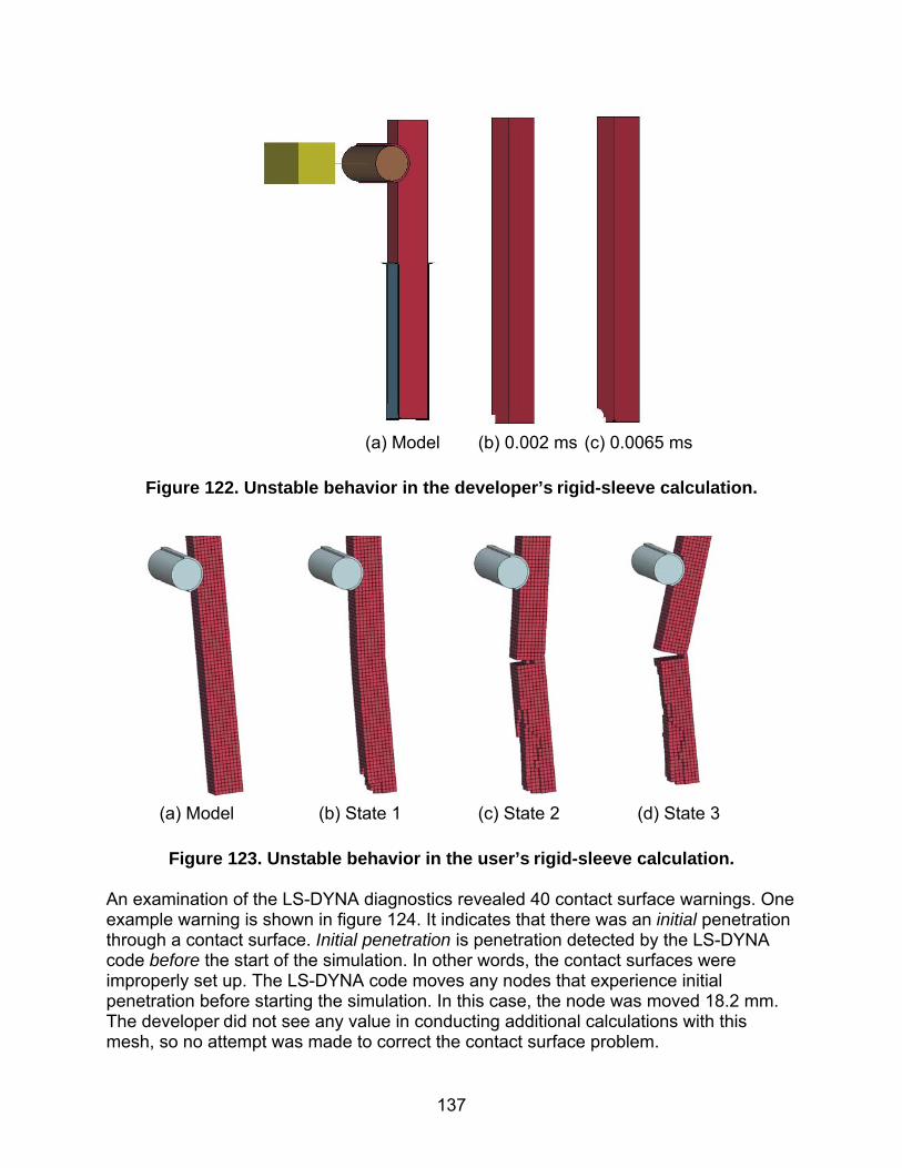
137

(a) Model (b) 0.002 ms (c) 0.0065 ms

Figure 122. Unstable behavior in the developer’s rigid-sleeve calculation.

(a) Model (b) State 1 (c) State 2 (d) State 3

Figure 123. Unstable behavior in the user’s rigid-sleeve calculation. An examination of the LS-DYNA diagnostics revealed 40 contact surface warnings. One example warning is shown in figure 124. It indicates that there was an initial penetration through a contact surface. Initial penetration is penetration detected by the LS-DYNA code before the start of the simulation. In other words, the contact surfaces were improperly set up. The LS-DYNA code moves any nodes that experience initial penetration before starting the simulation. In this case, the node was moved 18.2 mm. The developer did not see any value in conducting additional calculations with this mesh, so no attempt was made to correct the contact surface problem.

138

Figure 124. LS-DYNA diagnostics indicate that a contact surface is improperly positioned and requires movement of nodes prior to running the simulation.

Runs Conducted With Different LS-DYNA Releases Version 960 Using Interface: No instabilities occurred in the developer’s calculations, in which the wood model was interfaced with LS-DYNA as a user-defined material model. All runs were conducted on a Compact Alpha system using UNIX. In addition, penetration at the sharp corner between the liner and the wood post was not nearly as significant as that calculated with beta version 970, revision 1877 (PC using Windows). This is demonstrated by comparing figure 125 with figure 116.

C

(a) 25 ms (b) 38 ms Figure 125. The liner does not penetrate the post in calculations conducted with

LS-DYNA, version 960.

*** Warning - initial penetration through contact surface interface # = 2 interface type = 5 moved node = 9998 closest node = 15078 segment = 1372 penetration = -0.1658895E+02 normal = 0.0000000E+00 0.1000000E+01 0.0000000E+00 node 9998 old x,y,z = 0.1005000E+03 0.5841105E+02 -0.7810679E+03 node 9998 s,t = -0.6009506E+00 -0.1000000E+01 segment data: 15014 0.9999900E+02 0.7500000E+02 -0.7760000E+03 15077 0.9999900E+02 0.7500000E+02 -0.8014000E+03 15078 0.7499900E+02 0.7500000E+02 -0.8014000E+03 15015 0.7499900E+02 0.7500000E+02 -0.7760000E+03 *** Warning-node 9998 of contact interface 2 moved -0.182E+02

139

Beta Version 970, Revision 1553: With one exception, instabilities did not occur in the developer’s calculations (with or without time-step reduction), all of which used the wood model implemented as material model 143. The exception was an error termination following initialization when the *CONTACT_SINGLE_SURFACE formulation was requested. The error was out-of-range velocities applied to the nodes of the wood post at time zero, even though the post was not impacted by the bogie until about 0.5 ms. Beta Version 970, Revision 1877: Instabilities sometimes occurred in the developer’s calculations if the critical time step for contact stability was violated. One instability also occurred in the liner if the *CONTACT_SINGLE_SURFACE formulation was requested, even though the time step was set below that needed for contact surface stability. Summary In summary, all calculations except one exhibited stable behavior when conducted with the time step set below that needed for stable contact surface behavior. Instabilities may (but do not always) occur if the time step for stable contact surface behavior is exceeded. Instabilities are not identical and reproducible from computer platform to computer platform. The one instability that we were unable to control occurred in the elastic liner when using the *CONTACT_SINGLE_SURFACE formulation. However, having instability with one type of surface is not an insurmountable problem. With more than 25 contact surface types available in the LS-DYNA code, the user has a variety of methods available to specify and control contact surface stability and penetration.

141

18 REFERENCES 1. LS-DYNA Keyword User’s Manual, Volumes 1 and 2, Version 960, Livermore

Software Technology Corporation, Livermore, CA, 2001. 2. Murray, Y.D., Manual for LS-DYNA Wood Material Model 143, Report No. FHWA-

HRT-04-097, Federal Highway Administration, 2004. 3. Lewis, B.A., Manual for LS-DYNA Soil Material Model 147, Report No. FHWA-

HRT-04-095, Federal Highway Administration, 2004. 4. Reid, J.D., B.A. Coon, B.A. Lewis, S.H. Sutherland, and Y.D. Murray, Evaluation of

LS-DYNA Soil Material Model 147, Report No. FHWA-HRT-04-094, Federal Highway Administration, 2004.

5. Green, D.W., and D.E. Kretschmann, “Moisture Content and Properties of Clear

Southern Pine,” Research Paper FPL-RP-431, Forest Products Laboratory, U.S. Department of Agriculture, 1994.

6. Green, D.W., and D.E. Kretschmann, “Properties and Grading of Southern Pine

Timbers,” Forest Products Journal, Vol. 45, No. 9, September 1997, pp. 78-85. 7. Rohde, J.R., and J. Reid, “Evaluation of the Performance Criteria for Wood Posts

in Strong-Post W-Beam Guardrail,” TRB Paper 97-1206, Transportation Research Board, January 1997.

8. Coon, B., “Methodology for Digital Filtering of Data Using DaDisp,” Midwest

Roadside Safety Facility internal document, Lincoln, NE, December 1999. 9. Reid, S.R., and C. Peng, “Dynamic Uniaxial Crushing of Wood,” International

Journal of Impact Engineering, Vol. 19, Nos. 5-6, 1997, pp. 531-570. 10. Bragov, A., and A.K. Lomunov, “Dynamic Properties of Some Wood Species,”

Journal de Physique IV, France 7, 1997, Colloque C3, Supplement au Journal de Physique III d’août, [Journal of Physics IV, France 7, C3 Conference, Supplement to the Journal of Physics III for August],1997.

11. Bodig, J., and B.A. Jayne, Mechanics of Wood and Wood Composites, Krieger Publishing Company, Malabar, FL, 1993.