Evaluation of local similarity theory in the wintertimenocturnal boundary layer over heterogeneous surface

Babić, Karmen; Rotach, Mathias W.; Bencetić Klaić, Zvjezdana

Source / Izvornik: Agricultural and Forest Meteorology, 2016, 228-229, 164 - 179

Journal article, Accepted versionRad u časopisu, Završna verzija rukopisa prihvaćena za objavljivanje (postprint)

https://doi.org/10.1016/j.agrformet.2016.07.002

Permanent link / Trajna poveznica: https://urn.nsk.hr/urn:nbn:hr:217:291336

Rights / Prava: In copyright

Download date / Datum preuzimanja: 2022-03-20

Repository / Repozitorij:

Repository of Faculty of Science - University of Zagreb

http://dx.doi.org/10.1016/j.agrformet.2016.07.002

Evaluation of Local Similarity Theory in the Wintertime Nocturnal Boundary Layer over 1

Heterogeneous Surface 2

Karmen Babić1, Mathias W. Rotach

2 and Zvjezdana B. Klaić

1 3

1 Department of Geophysics, Faculty of Science, University of Zagreb, Zagreb, Croatia. 4

2 Institute of Atmospheric and Cryospheric Sciences, University of Innsbruck, Innsbruck, Austria. 5

6

Abstract: The local scaling approach was examined based on the multi-level measurements of atmospheric turbulence 7

in the wintertime (December 2008 February 2009) stable atmospheric boundary layer (SBL) established over a 8

heterogeneous surface influenced by mixed agricultural, industrial and forest surfaces. The heterogeneity of the surface 9

was characterized by spatial variability of both roughness and topography. Nieuwstadt's local scaling approach was 10

found to be suitable for the representation of all three wind velocity components. For neutral conditions, values of all 11

three non-dimensional velocity variances were found to be smaller at the lowest measurement level and larger at higher 12

levels in comparison to classical values found over flat terrain. Influence of surface heterogeneity was reflected in the 13

ratio of observed dimensionless standard deviation of the vertical wind component and corresponding values of 14

commonly used similarity formulas for flat and homogeneous terrain showing considerable variation with wind 15

direction. The roughness sublayer influenced wind variances, and consequently the turbulent kinetic energy and 16

correlation coefficients at the lowest measurement level, but not the wind shear profile. The observations support the 17

classical linear expressions for the dimensionless wind shear ( ) even over inhomogeneous terrain after removing 18

data points associated with the flux Richardson number (Rf) greater than 0.25. Leveling-off of at higher stabilities 19

was found to be a result of the large number of data characterized by small-scale turbulence (Rf > 0.25). Deviations 20

from linear expressions were shown to be mainly due to this small-scale turbulence rather than due to the surface 21

heterogeneities, supporting the universality of this relationship. Additionally, the flux-gradient dependence on stability 22

did not show different behavior for different wind regimes, indicating that the stability parameter is sufficient predictor 23

for flux-gradient relationship. Data followed local z-less scaling for when the prerequisite Rf ≤0.25 was imposed. 24

25

Key words: Stable boundary layer, Local scaling, Forest canopy, Roughness sublayer, Turbulent kinetic energy 26

Corresponding author at: Department of Geophysics, Faculty of Science, University of Zagreb, 27

Horvatovac 95, 10000 Zagreb, Croatia. Tel: +385 1 460 59 26. 28

E-mail address: babick@gfz.hr (K. Babić) 29

©2016. This manuscript version is made available under the CC-BY-NC-ND 4.0 licence 30

http://creativecommons.org/licences/by-nc-nd/4.0/31

2

1. Introduction 32

Stable atmospheric boundary layers (SBLs) are influenced by many independent forcings, such as, 33

(sub)mesoscale motions, which act on a variety of time and space scales, net radiative cooling, temperature 34

advection, surface roughness and surface heterogeneity (Mahrt, 2014) enhancing the complexities and 35

posing challenges in the study of the SBL. The fate of pollutants in the boundary layer is strongly affected 36

by turbulence which is extremely complicated in complex terrain and over heterogeneous surfaces. 37

Moreover, due to weak turbulence the SBL is generally favorable for the establishment of air pollution 38

episodes. Atmospheric dispersion models, used for air quality studies, as well as high-resolution regional 39

models use similarity scaling to model flow characteristics and dispersion in such environments. 40

Monin-Obukhov similarity theory (MOST) (Monin and Obukhov, 1954; Obukhov, 1946) relates surface 41

turbulent fluxes to vertical gradients, variances and scaling parameters. The assumptions underlying MOST 42

include stationary atmospheric turbulence, surface homogeneity and the existence of an inertial sublayer 43

(that is, surface layer, SL). Relations between these parameters (Businger et al., 1971; Dyer, 1974) are based 44

on several experimental campaigns conducted over horizontally homogeneous and flat (HHF) surfaces 45

(Kaimal and Wyngaard, 1990), where the original assumptions are considered to be met. Originally, MOST 46

was based on surface fluxes, which were assumed to be constant with height, and equal to surface values 47

within the SL (also referred to as constant-flux layer). In the unstable boundary layer, MOST has been 48

extensively studied and proven useful in relating turbulent fluxes to profiles (Businger et al., 1971; Dyer, 49

1974; Wyngaard and Coté, 1972). However, the applicability of MOST in the stable SL (e.g. Cheng et al., 50

2005; Trini Castelli and Falabino, 2013) and over complex (Babić et al., 2016; Nadeau et al., 2013; Stiperski 51

and Rotach, 2016) and heterogeneous surfaces is still an open issue due to many difficulties when applying 52

traditional scaling rules since MOST assumptions may not be fulfilled. Nieuwstadt (1984) extended Monin-53

Obukhov similarity in terms of a local scaling approach. This regime represents the extension of MOST 54

above the SL. Accordingly, all MOST variables are based on the local fluxes at a certain height z instead of 55

using surface values. As MOST should be valid over flat and homogeneous terrain, studies of the SBL in 56

terms of surface layer and local scaling approaches were made over areas characterized by long and uniform 57

fetch conditions, such as, Greenland, Arctic pack ice and Antarctica (Forrer and Rotach, 1997; Grachev et 58

al., 2013, 2007; Sanz Rodrigo and Anderson, 2013). Forrer and Rotach (1997) concluded that local scaling is 59

superior over surface layer scaling. This was mainly due to the fact that surface layer over an ice sheet, with 60

3

continuously stable stratification, can be very shallow (< 10 m). Moreover, for cases of strong stability, non-61

dimensional similarity functions for momentum and heat were in agreement with the results obtained from 62

the local scaling approach. Grachev et al. (2013) examined limits of applicability of local similarity theory in 63

the SBL by revisiting the concept of a critical Richardson number. 64

Even modest surface heterogeneity can significantly influence the nocturnal boundary layer (NBL) and 65

lead to turbulence at higher Richardson numbers in comparison with homogeneous surfaces (Derbyshire, 66

1995). Since the earth's solid surfaces are mainly heterogeneous (at least to a certain degree), the interest in 67

flow and turbulence characteristics over complex surfaces has increased in recent decades. Moreover, a 68

proper representation of turbulence is particularly important for parameterization of surface-atmosphere 69

exchange processes in atmospheric models (e.g., dispersion, numerical weather prediction or regional 70

models). The turbulence characteristics have been studied through direct measurements for different 71

complex surfaces including, complex forest sites (e.g. Dellwik and Jensen, 2005; Nakamura and Mahrt, 72

2001; Rannik, 1998), agricultural fields, such as, apple orchard (e.g. de Franceschi et al., 2009) or rice 73

plantation (e.g. Moraes et al., 2005), metre-scale inhomogeneity (Andreas et al., 1998a), urban areas (e.g. 74

Fortuniak et al., 2013; Wood et al., 2010), and complex mountainous terrains (e.g. Rotach et al., 2008), 75

addressing to both valley floors (e.g. de Franceschi et al., 2009; Moraes et al., 2005; Rotach et al., 2004) and 76

steep slopes (Nadeau et al., 2013; Stiperski and Rotach, 2016). However, most of these studies are 77

associated with flows over homogeneous surfaces. In recent years much effort has been put into simulations 78

of turbulent fluxes over relatively heterogeneous surfaces using large-eddy simulations (LES, e.g. Calaf et 79

al., 2014). Bou-Zeid et al. (2007) used LES over surfaces with varying roughness lengths to assess the 80

parameterization for the equivalent surface roughness and the blending height in the neutral boundary layer 81

at regional scales. Large eddy simulations of surface heterogeneity effects on regional scale fluxes and 82

turbulent mixing in the stably stratified boundary layers were studied by Miller and Stoll, 2013; Mironov 83

and Sullivan, 2010; Stoll and Porté-Agel, 2008. 84

The vertical structure of the atmospheric boundary layer is traditionally partitioned into a SL, an outer 85

layer and the entrainment zone (e.g. Mahrt, 2000). The SL, in turn, is subdivided into a canopy layer (CL), a 86

roughness sublayer (RSL) and inertial sublayer. Over surfaces with small roughness elements the latter, 87

which corresponds to the true equilibrium layer, is often identified with SL. These concepts are less 88

applicable over heterogeneous surfaces but for the SBL they provide, nevertheless, a useful starting point. 89

4

Above very rough surfaces, such as forests or agricultural crops, the RSL has a non-negligible extension. 90

Due to the influence of individual roughness elements on the flow within the RSL (e.g. Finnigan, 2000; 91

Katul et al., 1999), MOST is not widely accepted. The existence of large-scale coherent turbulent structures 92

within the RSL, which are generated at the canopy top through an inviscid instability mechanism (Raupach 93

et al., 1996), is thought to be a reason for the failure of standard flux-gradient relationships (Harman and 94

Finnigan, 2010). 95

In the scientific community substantial effort was made to address MOST in different conditions. Most 96

of the observational studies are based on measurements from a single tower, and sometimes they result in 97

inconsistent conclusions on the applicability of similarity theory. These inconsistencies are mostly found for 98

studies of MOST in complex terrain (e.g. de Franceschi et al., 2009; Kral et al., 2014; Martins et al., 2009; 99

Nadeau et al., 2013) or for small scale turbulence for which z-less scaling regime should apply (e.g. Basu et 100

al., 2006; Cheng and Brutsaert, 2005; Forrer and Rotach, 1997; Grachev et al., 2013; Pahlow et al., 2001). 101

The main objective of the present paper is to examine the applicability of local similarity scaling over a 102

heterogeneous terrain influenced by a mixture of forest, agricultural and industrial surfaces, based on multi-103

level turbulence observations in the wintertime SBL. Many of the above mentioned studies in complex 104

terrain are mainly characterized by homogeneous surface roughness, while studies over heterogeneous and 105

patchy vegetation are still scarce in the literature. Additionally, this paper relates to the approach of Grachev 106

et al. (2013), who investigated the limits of applicability of local similarity theory in the SBL over idealized 107

homogeneous surface of the Arctic pack ice. In the present work we use their approach to distinguish 108

between Kolmogorov and non-Kolmogorov turbulence, and consequently, to investigate whether classical 109

linear flux-gradient relationships can be applied for non-homogeneous surfaces. The paper is organized as 110

follows: in Section 2, we give a brief overview of the local scaling approach. In Section 3, we describe the 111

measurement site and measurements and we provide a description of post processing procedures. Section 4 112

contains our results for scaled standard deviations of wind components, turbulent kinetic energy, turbulent 113

exchange coefficients and non-dimensional wind profile. A summary and conclusions are given in Section 5. 114

115

2. Local scaling 116

Holtslag and Nieuwstadt (1986) presented an overview of scaling regimes for the SBL. Each of the 117

scaling regimes is characterized by different scaling parameters. The turbulence in the SL can be described 118

5

by MOST with surfaces fluxes of heat and momentum and the height z as scaling parameters. In this layer 119

the relevant scaling parameter is the Obukhov length L (Obukhov, 1946), given by 120

(1)

where is the surface friction velocity, is the surface kinematic heat 121

flux, is the virtual potential temperature, g is the acceleration due to the gravity, k=0.4 is the von Kármán 122

constant. Overbars and primes denote time averaging and fluctuating quantities, respectively. 123

Above the SL, the local scaling regime applies, a regime proposed by Nieuwstadt (1984). According to 124

Nieuwstad’s local similarity approach, properly scaled turbulence statistics should solely be a function of the 125

local stability parameter , where z is the measurement height, d is zero-plane displacement 126

height and Λ is the local Obukhov length. Even if Nieuwstadt (1984) was not referring to rough surfaces, we 127

have introduced d as we will be concerned with data from a site where the canopy height is non-negligible. 128

In the local scaling framework, the local Obukhov length is based on the local fluxes at height z and varies 129

with height 130

(2)

where indicates local friction velocity and is the local heat flux. Holtslag and Nieuwstadt (1986, 131

their Fig. 2) showed that in the part of the SBL which encompasses a layer between 10 and 50 % of the total 132

BL height at neutral stability and is exponentially decreasing with increasing stability, Λ L. This indicates 133

that the use of (z-d)/Λ, which is required by local scaling, is almost equivalent to the SL scaling parameter (z-134

d)/L. Therefore, the local scaling approach can be viewed as an extension of MOST for the entire SBL. 135

For large values of ( ), the dependence on z disappears because stable stratification restricts 136

vertical motion causing turbulence scales to be very small. Wyngaard and Coté (1972) named this limit 137

“local z-less stratification” (height-independent). Based on the observations from a tall tower (Cabauw), 138

Nieuwstadt (1984) found this limit to be for > 1. 139

Evaluation of second-order moments, especially of wind velocity standard deviations provides a good 140

understanding of turbulence statistics. According to similarity theory, dimensionless quantities should be 141

universal functions of the non-dimensional stability parameter. In the local scaling framework, standard 142

6

deviations of wind speed components , where denotes longitudinal, lateral and vertical 143

velocity components, respectively, are scaled as 144

(3)

where represents a set of universal similarity functions, different for each velocity component. In the 145

literature different formulations of the functions can be found. de Franceschi et al. (2009) presented a 146

comprehensive review of various formulations of functions suggested by different studies and for 147

different stabilities. A generally accepted form of the flux-variance similarity relationships in the stable 148

boundary layer is 149

(4)

where coefficients , and need to be found experimentally. Accordingly, the non-dimensional wind 150

shear defined as 151

(5)

where U is the mean wind speed, is also a unique function of stability. For neutral conditions (ζ = 0), 152

approaches unity. As the exact forms of the similarity functions are not predicted by similarity theory and 153

they should be determined from field experiments, many different formulations have been proposed based 154

on the data from different experiments (e.g. Beljaars and Holtslag, 1991; Cheng and Brutsaert, 2005; Dyer, 155

1974; Grachev et al., 2007; Sorbjan and Grachev, 2010). We will compare our results to the linear 156

relationship of Dyer (1974) obtained for the stable SL 157

(6)

where = 5. Högström (1988) modified several existing formulas for (and also for the non-158

dimensional temperature profile, ), in order to comply with his assumptions of and 159

. For Dyer's expression (6), he obtained a value . Additionally, we compare our results to the 160

non-linear stability function of Beljaars and Holtslag (1991) 161

(7)

where a = 1, b = 0.667, c = 5, d = 0.35, as expressions (6) and (7) are probably the most often used for 162

parameterization in numerical models. Both relationships were derived over flat and homogeneous terrain 163

using Obukhov length, which is based on surface values. While the first expression was derived and verified 164

7

by different experiments in the stability range 0 < z/L < 1, Eq. (7) is valid in strongly stable conditions were 165

the overestimation of the non-dimensional gradients is reduced. Linear equations for the stable SL together 166

with the relations for the unstable conditions are traditionally called Businger-Dyer relations (Businger et al., 167

1971; Dyer, 1974). Similar to the non-dimensional velocity variances we use the non-dimensional wind 168

shear in its local form (see Eq. (5)). 169

Another widely used stability parameter is the flux Richardson number, defined based on the vertical 170

gradient of wind speed 171

(8)

Grachev et al. (2013) argued that the upper limit for applicability of the local similarity theory is determined 172

by the inequalities and where is the gradient Richardson number. They found both 173

critical values to be equal to , with being the primary 174

threshold. The z-less concept requires that z cancels in Eqs. (4) and (6). As a result, a linear relationship for 175

the non-dimensional function is obtained, while non-dimensional functions asymptotically approach 176

constant values: 177

,

,

(9)

(10)

where and are experimentally determined coefficients. For convenience, throughout this paper we will 178

use the notation as all variables are based on local values. 179

180

3. Data and Methods 181

3.1. Site description 182

A 62 m high tower was located in the vicinity of the small industrial town Kutina, Croatia (tower 183

coordinates: 45o28'32"N, 16

o47'44"E). The tower was placed above a grassy surface and it was surrounded 184

by approximately 18 m high black walnut (Juglans nigra) trees. The closest trees are approximately 20 25 185

m away from the tower and they encompass an area of approximately 120 480 m2 (Fig. 1). The tower is 186

situated in a rather heterogeneous surrounding regarding both a larger spatial scale (Fig. 1a) and immediate 187

vicinity of the measurement site (on the order of 1 km distance, Fig. 1b). To the east of the tower, crop 188

8

fields, which extend to the aerial distance of more than 1 km, are found. South-southeast of the tower, about 189

800 m to 1.5 km distant a large petrochemical industry plant is placed. In a sector that encounters winds 190

from the north-northwest to the northeast, low, forested hills are located. They are covered with a dense 191

forest, while at lower elevations, cultivated orchards and vineyards are found. Foots of these hills are 192

roughly 1.3 km away from the measurement site. Thus, due to different surface roughness features 193

measurements in the SBL at the measuring site may be contaminated by local advective fluxes, drainage 194

flows and/or orographically-generated gravity waves. These features are related to (sub)mesoscale motions 195

which do not obey similarity scaling and are therefore removed from our data by the rigorous data quality 196

control and post-processing options as described later in the paper (Section 3.2.). We are thus focusing on 197

the micrometeorologically complex local site characteristics, which may be more typical for real sites than 198

the usually investigated homogeneous reference sites. 199

200

Fig. 1. (a) Topographic map with contour lines each 25 m of the area surrounding the measurement site (red 201

dot) representing inhomogeneous terrain on a larger spatial scale. (b) Google Maps image (Image © 2015 202

DigitalGlobe) of the observational site. Measurement tower is indicated with a red dot (45o28'32"N, 203

16o47'44"E). Light gray shaded areas correspond to wind directions depicted in Fig. 5. 204

205

Data used in this study were collected during wintertime (1 December 2008 28 February 2009) and 206

correspond to the nocturnal period from 1800 to 0600 local time. Turbulence measurements of three-207

dimensional wind and sonic temperature were continuously measured using identical WindMaster Pro (Gill 208

Instruments) ultrasonic anemometers that sampled at 20 Hz. Data were measured at five levels above the 209

9

canopy height, hereafter at level 1 (z1 = 20 m above the surface), level 2 (z2 = 32 m), level 3 (z3 = 40 m), 210

level 4 (z4 = 55 m) and level 5 (z5 = 62 m). Measurement levels were prescribed prior to the experiment 211

through existing tower infrastructure. Given the complicated and spatially inhomogeneous characteristics of 212

the measurement site, an idealized vertical structure is considered as a zero-order approach in the analysis. 213

Estimate of vertical layers for neutral conditions was done using different models available in the literature 214

and serves as a simple model for the interpretation of the results. For stably stratified conditions these 215

estimates will not be perfectly appropriate, but will provide the gross picture. 216

Conceptually, when the air flows over changing terrain, the downwind surface conditions are likely to 217

influence the measurements via internal boundary layers (IBLs), which grow in height ( ) with downwind 218

distance (Fig. 2) (e.g. Cheng and Castro, 2002; Dellwik and Jensen, 2005). Only the lowest portion of the 219

IBL (10%) is in equilibrium with the new surface (internal equilibrium layer, IEL) while the flow above the 220

IBL is in equilibrium with the upstream surface conditions. The IEL can, finally, be identified with the 221

inertial sublayer (IS). However, if the new surface is very rough its lower part must be considered as a RSL. 222

Within the upper part of the IEL, i.e. IS, turbulent fluxes are approximately constant with height, MOST is 223

valid and the mean wind speed follows the expected logarithmic profile. Within the RSL, the flow is 224

influenced by the distribution and structure of canopy elements (Monteith and Unsworth, 1990; Rotach and 225

Calanca, 2014), with momentum and scalars transported by turbulence, wake effects and molecular diffusion 226

(Malhi, 1996). Above the height of the IEL ( ) stress and fluxes start to decrease due to the upwind 227

influence. This layer is defined as a transition layer (Fig. 2). Due to the very tall roughness elements we use 228

the zero-plane displacement height (d) as our reference - hence the IBL is assumed to range from up 229

to . Ideally, after a long enough flow over the new surface the IBL fills the entire boundary layer. 230

Since we are interested in evaluating the degree to which local scaling applies under inhomogeneous fetch 231

conditions we map the idealized SBL structure to the IBL. The transition layer then becomes the outer part 232

of the inhomogeneously forced SBL. 233

We have estimated the length scales introduced above as follows: is estimated based on the model of 234

Cheng and Castro (2002) 235

, (11)

10

236

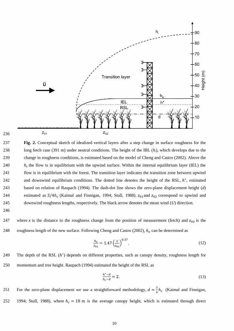
Fig. 2. Conceptual sketch of idealized vertical layers after a step change in surface roughness for the 237

long fetch case (391 m) under neutral conditions. The height of the IBL (hi), which develops due to the 238

change in roughness conditions, is estimated based on the model of Cheng and Castro (2002). Above the 239

the flow is in equilibrium with the upwind surface. Within the internal equilibrium layer (IEL) the 240

flow is in equilibrium with the forest. The transition layer indicates the transition zone between upwind 241

and downwind equilibrium conditions. The dotted line denotes the height of the RSL, , estimated 242

based on relation of Raupach (1994). The dash-dot line shows the zero-plane displacement height (d) 243

estimated as (Kaimal and Finnigan, 1994; Stull, 1988). and correspond to upwind and 244

downwind roughness lengths, respectively. The black arrow denotes the mean wind (U) direction. 245

246

where is the distance to the roughness change from the position of measurement (fetch) and is the 247

roughness length of the new surface. Following Cheng and Castro (2002), can be determined as 248

. (12)

The depth of the RSL ( ) depends on different properties, such as canopy density, roughness length for 249

momentum and tree height. Raupach (1994) estimated the height of the RSL as 250

. (13)

For the zero-plane displacement we use a straightforward methodology,

(Kaimal and Finnigan, 251

1994; Stull, 1988), where m is the average canopy height, which is estimated through direct 252

11

measurements (using laser distance meter). Additionally, for the walnut forest we used m (the lower 253

value for the roughness length over forest, m, according to Foken (2008), his Table 3.1). 254

The estimated height of the IBL at our site (Tab. 1) varied between 40 and 76 m for short ( 56 m) and 255

long ( 390 m) fetch conditions, respectively. Estimated values of at the location of the tower ranged 256

between 6.5 and 13.7 m according to Cheng and Castro (2002) for short and long fetch cases, respectively. 257

258

Table 1 259

Height of the equilibrium layer ( ) and of the internal boundary layer ( ) estimated based on the model of 260

the Cheng and Castro (2002) (Eqs. (11) and (12)) for different fetch (x) values corresponding to particular 261

wind directions (WD). Note that these heights indicate the height above the displacement height d. In the 262

determination of the fetch length, holes in the forest or corridors of vegetation other than forest were 263

disregarded if their size was small enough. 264

WD (deg) 30 60 90 120 150 180 210 240 270 300 330 360

x (m) 92 89 69 56 58 77 391 415 110 84 78 105

(m) 7.8 7.7 7.0 6.5 6.6 7.3 13.4 13.7 8.3 7.6 7.4 8.2

(m) 47 46 43 40 40 44 76 77 50 46 44 49

265

These estimates indicate that the second measurement level is above the IEL height ( ) for all 266

wind directions. Also, the height of the RSL at our measurement site is , that is, approximately 267

22.5 m. Using the above estimates, we find that level 1 is likely to be within the RSL for all wind directions. 268

For cases characterized with the short fetch, the IEL will most likely be within the RSL ( ), 269

while only for wind direction with large fetch conditions (200 250 deg) the growing equilibrium layer will 270

encompass the RSL and a thin IS will form. Levels 2 and 3 are in the transition layer for all wind directions, 271

while levels 4 and 5 are even above hi for the short fetches (105 175 deg). The highest measurement level 272

reflects the upwind surface conditions for fetches shorter than 100 m. Hence a potential RSL influence 273

should be detectable if level 1 behaves differently. If levels 2 5 do not show different behavior this can be 274

taken as an indication that our crude mapping assumption has some validity. 275

276

3.2. Post processing of the data 277

Instruments were mounted 3 m away from the triangular lattice tower (booms facing to the northeast) to 278

minimize any flow distortion effect by the tower. Considerable loss of data was incurred due to intermittent 279

12

winter icing or temporary instrument malfunction (Table 2). During this period, light nocturnal winds were 280

common at the site at the lowest measurement level (Fig. 3). We assume that the sonic temperature 281

, where T is the air temperature, is close to the virtual potential temperature . Automated 282

quality control procedures were not used since they may be too strict for the SBL analysis of weak 283

turbulence. Raw 20-Hz data were first divided into 30-min intervals. These intervals were checked for large 284

data gaps, and all 30-min intervals with more than 1% of missing data were omitted from further analyses. 285

After the consistency limits check, where we removed the data having unrealistically high values, spikes 286

(defined as data points within the time series which deviate more than four standard deviations from the 287

median value of the particular 30-min averaging window) were removed. If the number of spikes within the 288

30-min interval was less than 1% of the total data, spikes were replaced by linear interpolation from 289

neighboring values. We calculated angles of attack for each measurement and for each flux averaging 290

period, and flagged it if angles of attack exceeded 15 deg. The number of 30-min intervals available for the 291

further post-processing is labeled as “minimum QC” (Table 2). A cross-correlation correction of the time 292

series is already implemented in the Gill Instruments software. 293

Although double rotation of the data is the most commonly used to correct for sonic misalignment, 294

according to Mahrt (2011) and Mahrt et al. (2013) it should not be applied to SBL data under weak-wind 295

conditions. In the very stable boundary layer direction-dependent mean vertical motions may occur where 296

minor surface obstacles can significantly perturb the flow. In a setup like ours characterized by tall 297

vegetation and/or complex terrain, a non-zero 30-min mean vertical wind component may exist. In such 298

situations a planar fit (PF) method (Wilczak et al., 2001) would be better since it is based on an assumption 299

that the vertical wind component is equal to zero only over longer averaging periods. PF method performs a 300

multiple linear regression on the 30-min wind components to obtain the mean streamline plane (Aubinet et 301

al., 2012). This plane is based on the measurements made during the 88-night period for each of five levels 302

(Table 2). 303

13

304

Fig. 3. Wind roses at the measurement site for 30-min averaged data for the analyzed period (December 305

2008 February 2009). Levels 1 to 5 correspond to measurement heights of 20, 32, 40, 55 and 62 m above 306

the ground, respectively. 307

308

Basu et al. (2006) have shown that using an averaging window of inappropriate length can lead to false 309

conclusions concerning the behavior of the turbulence. In stable flows, use of an averaging time that is too 310

large leads to serious contamination of the computed flux by incidentally captured mesoscale motions 311

(Howell and Sun, 1999; Vickers and Mahrt, 2003). Previously Babić et al. (2012) applied two methods 312

based on Fourier analysis to determine an appropriate turbulence averaging time scale. In this study, we have 313

used a multiresolution flux decomposition (MFD) method (Howell and Mahrt, 1997) as described in Vickers 314

and Mahrt (2003). If the gap timescale is employed in the calculation of turbulent fluctuations, 315

contamination by mesoscale motions should be removed. Accordingly, in comparison with the use of an 316

arbitrary averaging time scale, similarity relationships should be improved. Here, based on the MFD method 317

we obtained a gap timescale of 100 sec, which is shorter than the previous value obtained by Babić et al. 318

(2012) for a single night case. Thus, a value of 100 sec was used here for a high-pass filtering of the time 319

series of raw u, v, w and Ts by applying a moving average. Since averaging over a longer time period (i.e. 30 320

or 60 min) reduces random flux errors in the case of relatively stationary turbulence, turbulent variances and 321

14

covariances in the present study correspond to 30-min averages. The mean wind speed and wind direction 322

were derived from the sonic anemometer data. 323

Stationarity of the time series is a fundamental assumption of similarity theory. Thus, it should be tested 324

prior to evaluation of similarity theory. Večenaj and De Wekker (2015) performed a comprehensive analysis 325

to detect non-stationarity based on various tests proposed in the literature. They found that the Foken and 326

Wichura (1996) test most often detects the largest number of non-stationary time intervals among all the 327

tests investigated. They concluded that non-stationarity significantly decreases if detrending or high-pass 328

filtering is applied, since highly non-stationarity (sub)mesoscale motions are removed by filtering. 329

Therefore, while testing non-stationarity of our datasets we first removed the linear trend for each 30-min 330

interval and then applied the Foken and Wichura (1996) test to the filtered time series. The percentage of 331

non-stationary periods for our dataset over heterogeneous terrain in the SBL varied between 20 and 30 % 332

depending on the level of observation (Tabe 2). This is slightly lower compared to studies of complex 333

mountainous terrain of Večenaj and De Wekker (2015) and Stiperski and Rotach (2016). 334

The statistical uncertainty (or sampling error) is inherent to every turbulence measurement. The 335

assessment of the statistical uncertainty is related to the averaging period. In order to estimate statistical 336

uncertainty we followed Stiperski and Rotach (2016). We performed this test on the time intervals which 337

were declared stationary by the foregoing test. The statistical uncertainty was estimated for the momentum 338

and heat fluxes, and for the variances. This was done for the fixed averaging period of 30-min. Although 339

over ideally flat and homogeneous surfaces one might choose 20% as a limit of statistical uncertainty, we 340

chose the 50% to assure both, high quality data sets, and a significantly large amount of input data for the 341

similarity analysis (Stiperski and Rotach, 2016). Thus, for the subsequent analysis only 30-min intervals 342

associated with statistical uncertainty below 50% were chosen. The uncertainty was largest for the kinematic 343

heat flux while for variances it was on average smaller than 50%. 344

Finally, following the QC recommendations by e.g. Klipp and Mahrt (2004) and Grachev et al. (2014) 345

we imposed the following thresholds: data with the local wind speed less than 0.2 ms-1

were omitted, while 346

minimum thresholds for the kinematic momentum flux, kinematic heat flux, and standard deviation of each 347

wind speed component were 0.001 ms-1

, 0.001 Kms-1

and 0.04 ms-1

, respectively. 348

349

350

15

Table 2 351

Number of 30-min intervals that satisfy the minimum QC (no large data gaps, no unrealistic values and no 352

spikes) within the observed period of 88 nights (out of a total of 2112 possible intervals). The number of 353

stationary and also the number of time intervals which are stationary and have uncertainty < 50% (used for 354

the analysis in this study) is given. 355

Crtieria Level 1 Level 2 Level 3 Level 4 Level 5

Minimum QC 647 802 1898 564 803

Stationary 482 576 1323 388 649

Stationary & Uncertainty % 342 388 760 225 357

356

357

Footprints are estimated and used in order to facilitate an interpretation of the results. Kljun et al. (2015) 358

presented a new parameterization for Flux Footprint Prediction (FFP) which has improved footprint 359

predictions for elevated measurement heights in stable stratification. Furthermore, the effect of the surface 360

roughness has been implemented into the scaling approach. It is based on a scaling approach of flux 361

footprint results of a thoroughly tested Lagrangian footprint model. A two-dimensional flux footprint model 362

of Kljun et al. (2015) (http://footprint.kljun.net/) was used to estimate the surface upwind of the 363

measurement tower that defined the fetch (flux footprint function) for the measurements at each level during 364

stable conditions. As input parameters we used the mean standard deviations of lateral wind component ( 365

= 0.40, 0.45, 0.41, 0.46 and 0.46 ms-1

for levels from 1 to 5, respectively), the mean local Obukhov lengths 366

( = 33, 28, 38, 45 and 39 m), the mean friction velocities ( = 0.23, 0.20, 0.19, 0.22 and 0.21 ms-1

) and 367

correspondingly, mean wind velocity for each measurement height (U = 1.9, 2.9, 3.1, 4.0 and 4.1 ms-1

). The 368

height of the SBL was set to 250 m since the result did not exhibit noticeable sensitivity to its choice. The 369

peak location of the footprint function, i.e. location of the maximum influence on the measurement, 370

increases with increasing height and varies between 19 and 405 m from the lowest to the highest 371

observational level, respectively. Additionally, the distance from the receptor that includes 90% of the area 372

influencing the measurement ( ) increases with height, where 65, 331, 570, 1260 and 1300 m, 373

correspond to levels 1 to 5, respectively. 374

375

3.3. Assesment of self-correlation 376

Monin-Obukhov as well as local similarity theory leads to self-correlation, because both predicted 377

variables and the predictors are functions of the same input quantities (Hicks, 1978). As an example, 378

prediction of (i = u, v, w) or in terms of the stability parameter contains self-correlation since both 379

16

or and ζ depend on . To test the role of self-correlation in our dataset, we followed the 380

approach of Mahrt (2003) as described in Klipp and Mahrt (2004), using 1000 random samples. Random 381

datasets were created by redistributing the values of , , and from the original dataset for 382

each measurement level. We used threshold values – mKs-1

and > 0.001 s-1

, as values 383

less than these are indistinguishable from zero. We repeated this process 1000 times and we calculated 384

corresponding 1000 random linear-correlation coefficients between and ζ and and ζ. The average of 385

these 1000 random correlation coefficients, , is a measure of self-correlation because random data no 386

longer have any physical meaning. The difference between the squared correlation coefficient of the original 387

dataset and

is proposed as a measure of the actual fraction of variance attributed to the 388

physical process. A very small value of the linear-correlation coefficient ( ) indicates no correlation 389

between compared variables. Mahrt (2014) stated that physical interpretation of results becomes ambiguous 390

when the self-correlation is of the same sign as the expected physical correlation. However, this test does not 391

seem to be appropriate for near-neutral and very stable cases (z-less limit), since and tend to 392

constant values, resulting in small (or even negative) correlation coefficients (Babić et al., 2016) 393

394

4. Results and Discussion 395

4.1. Flux-variance similarity 396

Variances of wind velocity components provide important information on turbulence intensity as well as 397

for the modeling of turbulent kinetic energy and transport. In this section we evaluate similarity of scaled 398

standard deviations of wind velocity components. Normalized standard deviations of wind components are 399

plotted as a function of the local stability parameter in Figs. 4 and 6. Figure 4 shows that scatter of the data 400

(gray symbols) increases with increasing height, where standard deviations of 0.27, 0.29, 0.41, 0.36 and 0.34 401

ms-1

correspond to levels from 1 to 5, respectively. Note that the number of data is the largest at level 3. 402

Moreover, after applying strict quality control criteria the scatter is substantially reduced (standard 403

deviations in the range 0.21 0.23 ms-1

). This is similar to results of Babić et al. (2016), and opposed to some 404

other studies in complex terrain (e.g. Fortuniak et al., 2013; Nadeau et al., 2013; Wood et al., 2010). 405

Stationary data that exceed our uncertainty threshold of 50% are presented in order to show the influence of 406

small fluxes (which are difficult to measure and hence uncertain) on the scatter of (presented as 407

gray symbols in Fig. 4). As seen from Fig. 4, this criterion is crucial for excluding the high values of the 408

17

scaled vertical wind variance in the strongly stable regime where z-less scaling should be valid. Without this 409

exclusion, an incorrect conclusion on the validity of z-less scaling might be drawn. In the subsequent 410

analysis these data are omitted and individual data as well as bin-averages in all figures correspond to data 411

(namely, wind variances and turbulent fluxes) which satisfy an uncertainty limit < 50%. 412

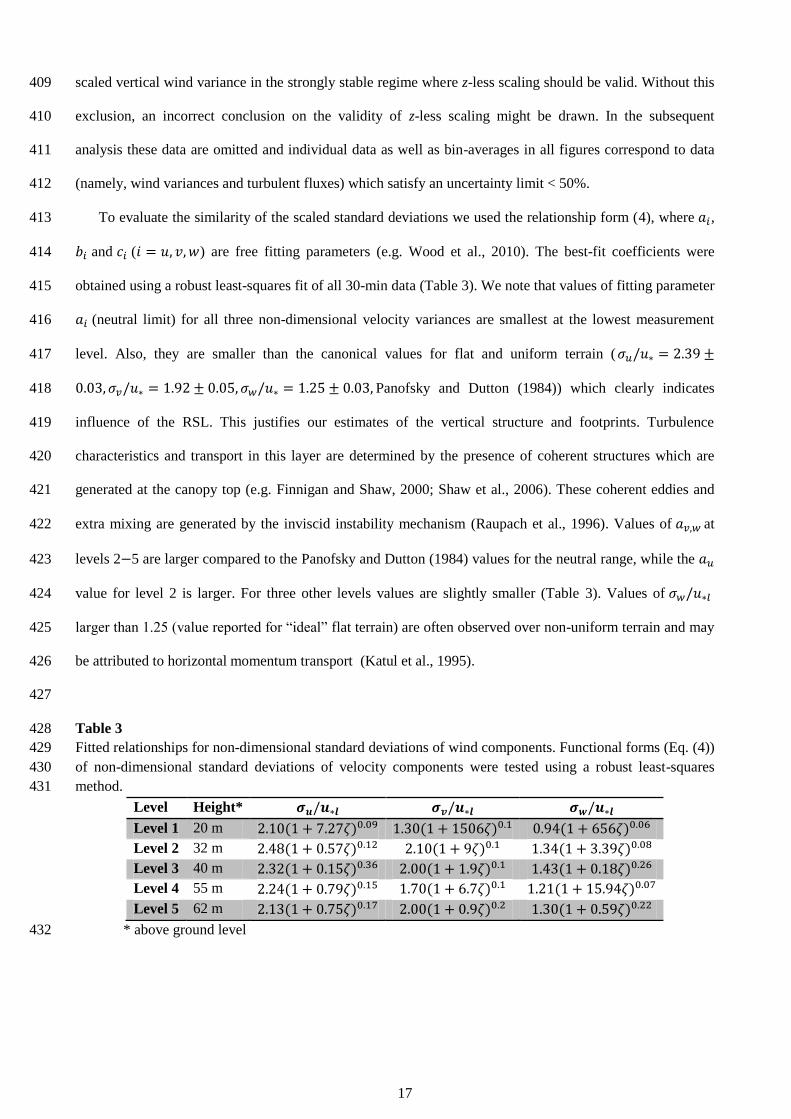
To evaluate the similarity of the scaled standard deviations we used the relationship form (4), where , 413

and ( ) are free fitting parameters (e.g. Wood et al., 2010). The best-fit coefficients were 414

obtained using a robust least-squares fit of all 30-min data (Table 3). We note that values of fitting parameter 415

(neutral limit) for all three non-dimensional velocity variances are smallest at the lowest measurement 416

level. Also, they are smaller than the canonical values for flat and uniform terrain ( 417

Panofsky and Dutton (1984)) which clearly indicates 418

influence of the RSL. This justifies our estimates of the vertical structure and footprints. Turbulence 419

characteristics and transport in this layer are determined by the presence of coherent structures which are 420

generated at the canopy top (e.g. Finnigan and Shaw, 2000; Shaw et al., 2006). These coherent eddies and 421

extra mixing are generated by the inviscid instability mechanism (Raupach et al., 1996). Values of at 422

levels 2 5 are larger compared to the Panofsky and Dutton (1984) values for the neutral range, while the 423

value for level 2 is larger. For three other levels values are slightly smaller (Table 3). Values of 424

larger than 1.25 (value reported for “ideal” flat terrain) are often observed over non-uniform terrain and may 425

be attributed to horizontal momentum transport (Katul et al., 1995). 426

427

Table 3 428

Fitted relationships for non-dimensional standard deviations of wind components. Functional forms (Eq. (4)) 429

of non-dimensional standard deviations of velocity components were tested using a robust least-squares 430

method. 431

Level Height*

Level 1 20 m

Level 2 32 m

Level 3 40 m

Level 4 55 m

Level 5 62 m

* above ground level 432

18

433

Fig. 4. Scaled standard deviation of vertical velocity fluctuations as a function of stability. Black solid line 434

( ) corresponds to: = 1.25(1 + 0.2ζ ) (Kaimal and Finnigan, 1994). Thin dashed line is an 435

extension for 1 < ζ < 10. Individual data at each level are shown as background symbols (gray symbols 436

represent stationary data points which exceed our uncertainty threshold of 50%). Error bars indicate one 437

standard deviation within each bin. The bin size is determined in a logarithmic scale using fifteen equally 438

spaced bins in the stability range 0.002 < ζ < 12.5. 439

440

19

As already mentioned, flux-variance similarity relationships are influenced by self-correlation. Small 441

values of fitted coefficients and/or indicate the best-fit curve which converges to a constant, i.e. . 442

Consequently, values of tend to converge to small values or even to zero, while

are usually 443

larger which leads to negative values of

. The same result was obtained by Babić et al. 444

(2016) and, as they pointed out, this presents a limitation of the method since it relies on the linear 445

correlation coefficient and does not allow for a reliable conclusion about self-correlation in the SBL. 446

Table 4 presents a review of published in the literature for different terrain characteristics 447

under neutral conditions. As already noted, dimensionless velocity variances in the RSL often exhibit 448

lower values in comparison with the flat terrain reference of Kaimal and Finnigan (1994). Our results for 449

at the lowest measurement level are in the range of values obtained within RSLs over forest 450

(Rannik, 1998) and urban (Rotach, 1993) areas. For levels 2 5, neutral values are close to those reported 451

by Moraes et al. (2005) and Wood et al. (2010). Using local scaling over the city of London 452

(measurements at 190 m above the ground), Wood et al. (2010) obtained near-neutral limits of 453

( ), which are in accordance with those reported for flat and homogeneous terrain where MOST 454

applies. They concluded that MOST was not complicated by too many factors, since London is quite flat 455

and there are consistent building heights across a wide area which produced a longer upwind fetch causing 456

the London boundary layer likely to be in equilibrium with the surface. Our results for are 457

furthermore consistent with Nieuwstadt (1984) who found it to be constant ( ) in the stability range 458

0.1 < ζ < 2. 459

Table 4 460

Comparison of neutral values for non-dimensional standard deviations of the wind from different studies. 461

Our near-neutral values correspond to the mean value of scaled standard deviations of wind in the range 462

0 0.05. 463

Reference Site description

Panofsky and Dutton (1984) Flat (reference) 2.39 1.92 1.25

Rotach (1993) Urban RSL 2.2 1.5 0.94

Rannik (1998) Pine forest RSL 2.25 1.82 1.33

Moraes et al. (2005) Complex (valley) 2.4 2.2 1.2

Wood et al. (2010) Urban BL 2.36 1.92 1.40

This study – Level 1 Heterogeneous 2.13 1.65 1.11

This study – Levels 2 5 Heterogeneous 2.41 2.08 1.37

464

20

4.1.1. Influence of the surface heterogeneity 465

Due to the fact that measurements were performed in a very heterogeneous landscape, we investigated 466

possible influences of different land-use types on turbulence statistics by considering changes for different 467

wind directions. Figure 5a shows the normalized standard deviation of the vertical wind component for each 468

observational level averaged over the entire stability range plotted versus wind direction. For the wind sector 469

45 90 deg there is no consistent increase of with height, possibly due to the fact that this narrow 470

wind sector is characterized through a sudden change of surface roughness (from agricultural fields to rough 471

forest) and also through a short fetch (some 70 m). This might indicate a more complex vertical structure 472

than depicted in Fig. 2 with flow which has not reached equilibrium yet. In the 300 360 deg wind sector, 473

the non-dimensional variance of the vertical wind has decreased values at the highest level in comparison 474

with values at levels 2 4. We hypothesize that this might indicate an influence of drainage flows from hills 475

located north of the measurement site. Drainage flows are thermally-driven and they occur during night over 476

sloping terrain often leading to the formation of low level jets. However, we do not have the necessary 477

information to substantiate this hypothesis. In the 190 260 deg sector, increases with height 478

indicating the flow which has adjusted to the new surface. This sector has the longest fetch (over 300 m) and 479

highly rough but uniform underlying surface (Figs. 1 and 2). 480

Observed changes of the normalized vertical wind variance with varying wind direction reflect the 481

influence of the surface inhomogeneity (and possibly topography). This influence is seen from the ratio of 482

observed non-dimensional variance of the vertical wind and corresponding values of commonly used 483

similarity formulas for in the “ideal” HHF terrain (e.g. Kaimal and Finnigan (1994), = 1.25(1 484

+ 0.2ζ )) in the stability range 0 < ζ < 1 (Fig. 5b). We observe that ratio of these two similarity functions at 485

the lowest measurement level is typically less than one, except for the flow from sectors 200 220 deg and 486

300 340 deg, which correspond to high roughness and long fetch (Fig. 1) and high wind speeds (Fig. 3), 487

respectively. At upper levels values of the ratio are larger than unity for wind azimuth ranges 488

55 80 deg, 170 230 deg and 300 360 deg (Fig. 5b). For these levels, the average ratio in 489

Fig. 5b varies between 0.96 and 1.33, which is similar to values obtained by Rannik (1998) in the study over 490

a forest, and the standard deviation for 10 deg wide bins is between 0.08 and 0.22. 491

21

492

Fig. 5. (a) Scaled standard deviation of vertical velocity fluctuations as a function of wind direction 493

(regardless of stability). Individual data points at each level corresponding to the particular wind sector are 494

shown as background symbols. Colored filled symbols correspond to bin averages over the entire stability 495

range at each observational level. Error bars indicate one standard deviation within each bin. (b) Observed 496

dimensionless standard deviation of vertical wind speed (for the lowest level and levels 2 5) relative to the 497

SL similarity prediction for HHF terrain (Kaimal and Finnigan (1994), denoted “HHF”) for stability 0 < ζ < 498

1, plotted versus wind direction. Shaded light gray areas indicate the wind azimuths which correspond to 499

undistorted surface conditions ( ). These correspond to wind directions 20 55 deg, 85 175 500

deg and 235 295 deg. The flow from other wind directions is considered as distorted. 501

502

Accordingly, we separately analyzed the velocity variances for different wind directions corresponding 503

to undistorted and distorted sectors, respectively. Based on undistorted wind directions 504

were defined to correspond to wind directions 20 55 deg, 85 175 deg and 235 295 deg (light gray shaded 505

area in Fig. 5b). All other wind directions were considered as distorted. The number of data within each 506

group was nearly evenly distributed except for the highest level. Namely, the percentage of data 507

corresponding to the undistorted sectors was 47, 56, 54, 52 and 64 % for levels from 1 to 5, respectively. 508

22

Figure 6 shows all three non-dimensional standard deviations at the lowest level and for levels 2 5 for 509

undistorted and distorted wind direction sectors separately. We note that the scatter is larger for horizontal 510

components than for the vertical wind component. Also, as one might expect the scatter is larger for the 511

distorted sectors compared to undistorted. Normalized variances at level 1 show much less dependence on 512

the wind direction compared to levels 2 5. This reflects the rather local RSL impact that determines the 513

statistics. That is, RSL turbulence appears to be affected by a fetch of less than 100 m from the tower as was 514

estimated by the flux-footprint model (Section 3.2.) rather than by the more distant complex surface. 515

Differences between distorted and undistorted sectors at this level are only found in the near-neutral regime 516

with larger magnitudes for the distorted sectors. For levels 2 5 we observe that the overall shape of the 517

curves for the two sectors is quite similar for all three wind variances. Dimensionless longitudinal and 518

vertical wind variances show higher values in the distorted sectors, while the lateral wind variance seems to 519

be independent on the wind direction. Similar to level 1, the lateral wind component shows a more 520

pronounced increase with stability than the longitudinal and vertical variances. The dimensionless vertical 521

wind variance in the undistorted sectors can be represented quite well with the similarity relationship valid 522

for flat and homogeneous terrain (Kaimal and Finnigan, 1994) in the stability range 0.01 < ζ < 1. Based on 523

modeled footprints particular wind sectors were related to corresponding surface types, accordingly. For the 524

undistorted wind directions 20 55 deg and 85 175 deg the underlying surface is represented with 525

agricultural fields, while the 235 295 deg sector represents somewhat rougher but quite uniform surface 526

covered mostly with the forest (Fig. 1). This implies that measurements at levels 2 5 corresponding to these 527

sectors correspond to a layer which is in equilibrium with the underlying surface of more uniform roughness. 528

In the strongly stable regime (for ζ > 1) the normalized variances show a tendency for a leveling-off , thus 529

suggesting that z-less scaling might be appropriate. This implies that even for highly inhomogeneous terrain 530

local scaling appears to be appropriate for all three velocity variances and that the local Obukhov length is 531

relevant length scale. Additionally, in the strong stability limit the z-less scaling seems to be appropriate for 532

longitudinal and vertical wind variances. 533

23

534

Fig. 6. Scaled standard deviations of (a) longitudinal, (b) lateral and (c) vertical velocity fluctuations as 535

functions of stability for level 1 (lower sub-panels) and levels 2 5 (upper sub-panels) for distorted (pink 536

triangles) and undistorted (gray diamonds) wind sectors. For explanation of other symbols see Fig. 4.537

538

24

4.1.2. Subcritical and supercritical turbulence regimes 539

Grachev et al. (2013) showed that the inertial subrange, associated with the Richardson-Kolmogorov 540

cascade, dies out when both the gradient and the flux Richardson number exceed a “critical value” of 541

approximately , with being the primary threshold. They argued that a 542

collapse of the inertial subrange is caused by the collapse of energy-containing/flux-carrying eddies. This 543

leads to the invalidity of Kaimal's spectral and cospectral similarity (Kaimal, 1973) and consequently, to 544

violations of flux-profile and flux-variance similarity. Correspondingly, Grachev et al. (2013) classified the 545

traditional SBL into two major regimes: subcritical and supercritical. In the former ( and 546

), turbulence statistics can be described by similarity theory and it is associated with Kolmogorov 547

turbulence. The supercritical regime ( and ) is related to small-scale, decaying, non-548

Kolmogorov turbulence, and strong influence of the Earth's rotation even near the surface. Figure 7 shows 549

the dependence of (Eq. (8)) on the local stability parameter at the measuring site. Dyer's parameterization 550

(Dyer, 1974) predicts an asymptotic limit to = 0.2 (solid black line), but this under-predicts for 551

higher stabilities for which increases above = 0.25 (supercritical regime). The range of stability 552

available for our analysis of the profile data is 0 < ζ < 5. For example, at levels 4 and 5, 40% and 50% of 553

data points have , respectively. Thus, higher levels, which correspond to higher stabilities, are 554

characterized by non-Kolmogorov turbulence. 555

Grachev et al. (2013) have found that was the primary threshold for . The 556

normalized standard deviation of the vertical wind speed was reported to become asymptotically constant in 557

the subcritical regime indicating consistency with z-less scaling in this regime. In the supercritical regime 558

was monotonically increasing with increasing stability. The turbulence characteristics at our site 559

(exemplified by the vertical velocity variance, Fig. 8) do not show a clear distinction in behavior between 560

sub- and supercritical regimes as was found in Grachev et al. (2013) and for the non-dimensional vertical 561

gradient of mean wind (Fig. 12). In the subcritical regime the number of data points at levels 2 5 with ζ > 1 562

is equal to 25 and is represented by only two bin averages. While Grachev et al. (2013) had a much broader 563

range of stability in both regimes (they obtained as small as 0.02 for the supercritical and up to 5 for the 564

subcritical regime, respectively), in our dataset the results for these two regimes are almost indistinguishable 565

(Fig. 8). Additionally, for the supercritical regime Grachev et al. (2013) observed an 566

567

25

568

Fig. 7. Stability dependence of the flux Richardson number for all five levels (shown with corresponding 569

symbol). Red squares and blue circles denote bin averages for the lowest level and for levels 2 5, 570

respectively. Error bars indicate one standard deviation within each bin. Number of data points inside each 571

bin for the two subsets of the data is also given. 572

573

574

Fig. 8. Scaled standard deviation of vertical velocity fluctuations as a function of stability. Data from the 575

lowermost level (squares) and for levels 2 5 (circles) in the subcritical (green) and supercritical (violet) 576

regime are presented. The dashed line is equal to 1.4 which is the mean value of all data for levels 2 5 in the 577

subcritical regime. The number of data in each regime is indicated with the corresponding color. 578

579

increase of in the range 3 < ζ < 100. For this regime we observed an increasing tendency for the two 580

highest levels, but this is probably not significant because of the small number of data and a restricted 581

26

stability range (upper limit is ζ = 5). Note that the number of data points here is much less compared to Figs. 582

4 and 6 because only 100 simultaneous 30-min intervals were available for the calculation of the flux 583

Richardson number. Similar results are found for the horizontal wind variances (not shown). 584

585

4.2. Turbulent kinetic energy 586

Estimation of turbulent kinetic energy (TKE) is very important for atmospheric numerical modeling, 587

since turbulent mixing is often parameterized using TKE. Here we investigate the TKE, defined as, 588

, which represents a turbulent kinetic energy per unit mass (Stull, 1988). Fig. 9 shows 589

scaled by the squared friction velocity. In numerical models which use 1.5-order closure or TKE closure, 590

TKE is predicted with a prognostic energy equation, and eddy viscosity is specified using the TKE and some 591

length scale. Since TKE is essentially the sum of variances (divided by 2), according to Kansas values for 592

neutral conditions (Kaimal and Finnigan, 1994), the value of scaled TKE is equal to 5.48 for HHF terrain. 593

Over HHF terrain in Antarctica, Sanz Rodrigo and Anderson (2013) found that for neutral to moderate 594

stabilities non-dimensional TKE is roughly constant up to ζ = 0.5. Above this value, non-dimensional TKE 595

grows until it reaches ζ = 10 (corresponding to the boundary-layer top), which is followed by an asymptotic 596

value for stronger stabilities (Fig. 9, dashed black line, Eq. (14)). They proposed a simple empirical 597

parameterization: 598

(14)

where is the neutral limit value and . 599

We fitted the above linear relation to our data from levels 2 5 in the stability range 0.006 < < 8.30 600

(Fig. 9, orange dashed line) using the least-squares method. Figure 9 shows a clear influence of the RSL on 601

the lowest measurement level, which does not correspond to the proposed near-linear expression (14). The 602

RSL influence also results in a reduced value of non-dimensional TKE for the neutral range ( 603

based on values from Tab. 4) in comparison with the value of 4.5 found by Sanz Rodrigo and Anderson 604

(2013). Their value is smaller than the reference value of 5.48 for HHF terrain probably due to higher air 605

density in the Antarctica causing reduced values of compared to mid-latitudes. We note that the 606

relation of the type given by Eq. (14) fits our data for levels 2 5 quite well (Fig. 9, orange dashed curve), 607

27

but with slightly different coefficients , which corresponds to a neutral value of , 608

and . The fitted neutral value of dimensionless TKE for levels 2 5 is close to the value of 6.01, 609

which is obtained based on values from Tab. 4. 610

611

612

Fig. 9. Dependence of non-dimensional turbulent kinetic energy on stability. The black dashed line is an 613

empirical fit (Eq. (14), Sanz Rodrigo and Anderson (2013)). Individual data at each level are shown in 614

background symbols, while red squares and blue circles represent bin-averages for the lowest and four 615

higher levels, respectively. Error bars indicate one standard deviation within each bin. The number of data 616

points within each bin for levels 2 5 is also indicated. The orange curve is a fit to our data for levels 2 5. 617

618

Similar to wind variances, analysis of the TKE with respect to wind direction shows similar distinction 619

between the distorted and undistorted sectors. While values of normalized TKE are similar for the two 620

sectors at the lowest level, at levels 2 5 magnitudes in the distorted sectors are larger. The dependence of 621

on the stability parameter can be represented with a linear relationship, but the best fit coefficients 622

are somewhat changed: and 0.14 and and 0.95 for undistorted and distorted sectors, 623

respectively (not shown). The behavior of the normalized TKE in the sub- and supercritical regime was 624

found to be consistent with the behavior of the normalized wind variances and no discernible difference 625

between these two regimes was observed (not shown). 626

28

4.3. Correlation coefficients 627

In order to estimate fluxes from mean wind and temperature as inputs for dispersion models it is useful 628

to use turbulent correlation coefficients. These coefficients are a measure of the efficiency of turbulent 629

transfer and are defined as 630

(15)

(16)

where and are correlation coefficients for momentum and heat transfer, respectively. Figure 10 631

shows momentum and heat flux correlation coefficients estimated for the lowest and the four higher 632

measurement levels. For strong stratification we obtained smaller values of the correlation coefficients for 633

momentum, but they increase quite steeply while approaching neutral conditions. This was also observed in 634

both an urban (e.g. Wood et al., 2010) and a rural dataset (e.g. Conangla et al., 2008). Additionally, 635

exhibits the same behavior with respect to the stability when analyzed for different wind azimuths. The 636

magnitude of the momentum correlation coefficient is larger for the undistorted sector compared to distorted 637

in the stability range 0 < ζ < 1 in the whole measurement layer (not shown). The stability-averaged 638

momentum flux correlation coefficient values are between 0.23 and 0.46 at level 1 (Fig. 10a) and a similar 639

range was observed for undistorted (0.22 0.51) and distorted (0.25 0.45) wind sectors. These values are 640

similar to those obtained by Marques Filho et al. (2008). For levels 2 5, the values of are somewhat 641

smaller compared to level 1 and are in the range 0.14 0.34 (Fig. 10a), and they are similar to those obtained 642

for the distorted wind sectors: 0.16 0.31 (not shown), which is in the range of values observed over 643

generally rougher urban surfaces (Wood et al., 2010). 644

The correlation coefficient for heat exhibits larger values for 0.1 for levels 2 5, and it decreases 645

while approaching neutral conditions. The correlation coefficient for heat is between 0.10 and 0.26, which is 646

similar to values reported in other studies (Marques Filho et al., 2008; Wood et al., 2010). Additionally, no 647

discernible dependence on wind direction was found for mostly due to the large scatter of the data (not 648

shown). Mean values of the momentum and heat flux correlation coefficients over the entire measurement 649

layer, and for all stabilities, are equal to 0.26 and 0.24, respectively. Also, no discernible difference in 650

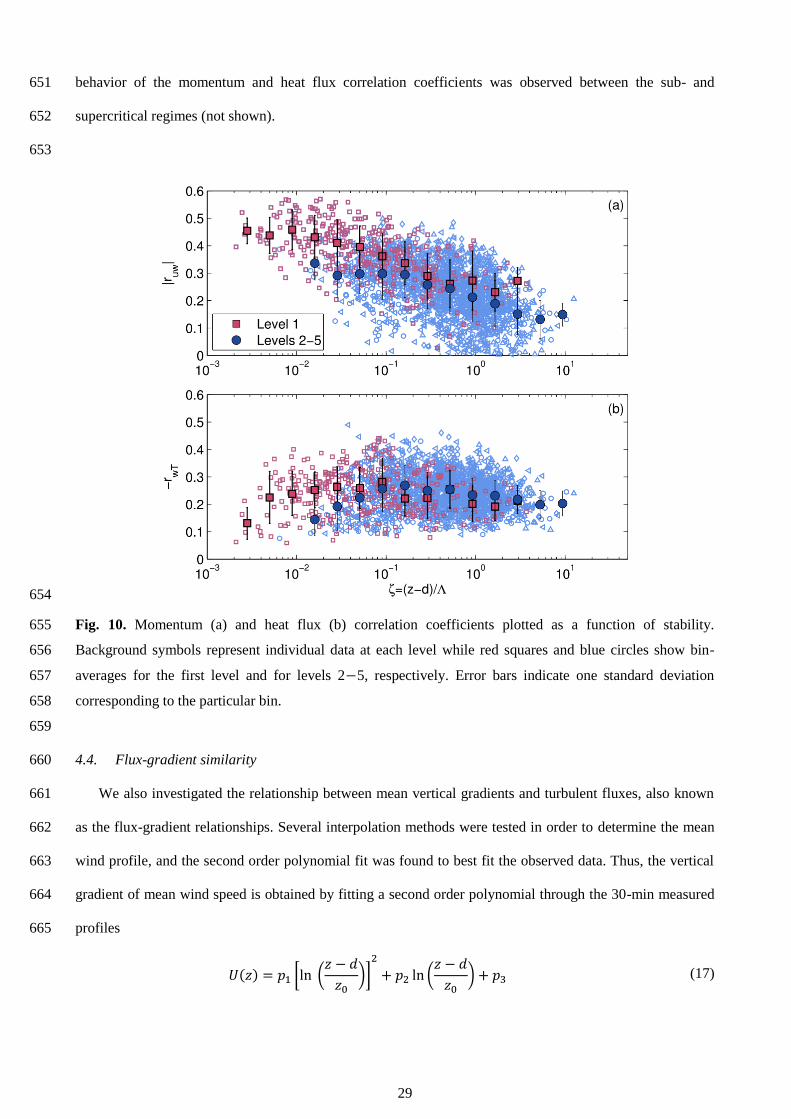
29

behavior of the momentum and heat flux correlation coefficients was observed between the sub- and 651

supercritical regimes (not shown). 652

653

654

Fig. 10. Momentum (a) and heat flux (b) correlation coefficients plotted as a function of stability. 655

Background symbols represent individual data at each level while red squares and blue circles show bin-656

averages for the first level and for levels 2 5, respectively. Error bars indicate one standard deviation 657

corresponding to the particular bin. 658

659

4.4. Flux-gradient similarity 660

We also investigated the relationship between mean vertical gradients and turbulent fluxes, also known 661

as the flux-gradient relationships. Several interpolation methods were tested in order to determine the mean 662

wind profile, and the second order polynomial fit was found to best fit the observed data. Thus, the vertical 663

gradient of mean wind speed is obtained by fitting a second order polynomial through the 30-min measured 664

profiles 665

(17)

30

and by evaluating a derivative with respect to z for each measurement level. The second order polynomial fit 666

is widely used for measurements within the roughness sublayer (e.g. Dellwik and Jensen, 2005; Rotach, 667

1993) as well as within the inertial sublayer (e.g. Forrer and Rotach, 1997; Grachev et al., 2013). Only about 668

one hundred simultaneous 30-min intervals were available from each measurement level for the profile 669

analysis. Results of the variance and TKE analyses showed a different behavior of the first level in 670

comparison with all the others. In order to investigate whether there is a difference in the flux-gradient 671

relationship as well, the data from the first level and levels 2 5 are presented separately (Fig. 11). For our 672

dataset no discernible difference of between level 1 and levels 2 5 can be observed. Almost all data at 673

the first measurement level are within the stability range and tends to a constant value of 1 674

when approaching near-neutral conditions. Quite diverse results concerning the value of in the RSL in 675

the near-neutral conditions can be found in the literature. While in some studies of flux-gradient similarity 676

within the forest RSL, was found to be less than unity in the near-neutral range (e.g. Högström et al., 677

1989; Mölder et al., 1999; Raupach, 1979; Thom et al., 1975), other studies indicate that is close to unity 678

(e.g. Bosveld, 1997; Simpson et al., 1998; Dellwik and Jensen, 2005; Nakamura and Mahrt, 2001). Bosveld 679

(1997) found that momentum and heat eddy diffusivities differ in magnitude in neutral conditions. This 680

means that, with increasing canopy density, heat exchange remains enhanced in the RSL, whereas 681

momentum exchange approaches surface-layer values. Dellwik and Jensen (2005) observed an increase of 682

in the RSL in neutral conditions over fetch-limited deciduous forest due to the increased wind gradients 683

directly above the canopy top. In previous studies reporting and having mostly been conducted over 684

pine forests (which compared to a closed deciduous forest have less biomass in the top of the canopy) the 685

observed wind profile close to the three tops was less steep. 686

The previous sections have revealed clear differences in the flux-variance relationships between level 1 and 687

levels 2-5 (i.e., the RSL and the transition layer, respectively) at the present site. In contrast, no significant 688

difference is observed for the flux-gradient relationship. Similar results were reported by Katul et al. (1995) 689

who pointed out that inhomogeneity in the RSL impacts variances but not necessarily fluxes. Following this 690

line, our results seem to indicate that surface characteristics at our site are influencing the strength of 691

turbulent mixing and the wind gradient in the same way. This conclusion is additionally corroborated by the 692

results of the analysis for different wind sectors as no dependence on the wind direction was found for the 693

non-dimensional gradient of wind speed (not shown). 694

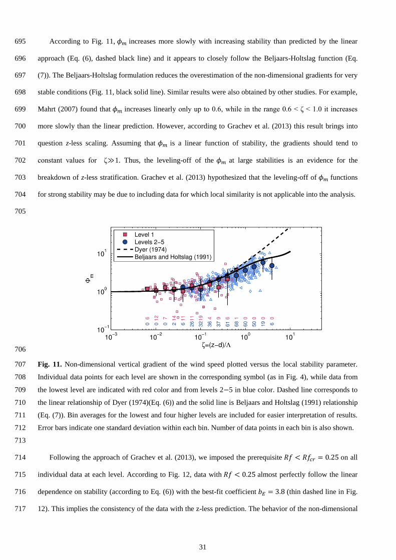
31

According to Fig. 11, increases more slowly with increasing stability than predicted by the linear 695

approach (Eq. (6), dashed black line) and it appears to closely follow the Beljaars-Holtslag function (Eq. 696

(7)). The Beljaars-Holtslag formulation reduces the overestimation of the non-dimensional gradients for very 697

stable conditions (Fig. 11, black solid line). Similar results were also obtained by other studies. For example, 698

Mahrt (2007) found that increases linearly only up to 0.6, while in the range 0.6 < ζ < 1.0 it increases 699

more slowly than the linear prediction. However, according to Grachev et al. (2013) this result brings into 700

question z-less scaling. Assuming that is a linear function of stability, the gradients should tend to 701

constant values for ζ 1. Thus, the leveling-off of the at large stabilities is an evidence for the 702

breakdown of z-less stratification. Grachev et al. (2013) hypothesized that the leveling-off of functions 703

for strong stability may be due to including data for which local similarity is not applicable into the analysis. 704

705

706

Fig. 11. Non-dimensional vertical gradient of the wind speed plotted versus the local stability parameter. 707

Individual data points for each level are shown in the corresponding symbol (as in Fig. 4), while data from 708

the lowest level are indicated with red color and from levels 2 5 in blue color. Dashed line corresponds to 709

the linear relationship of Dyer (1974)(Eq. (6)) and the solid line is Beljaars and Holtslag (1991) relationship 710

(Eq. (7)). Bin averages for the lowest and four higher levels are included for easier interpretation of results. 711

Error bars indicate one standard deviation within each bin. Number of data points in each bin is also shown. 712

713

Following the approach of Grachev et al. (2013), we imposed the prerequisite on all 714

individual data at each level. According to Fig. 12, data with almost perfectly follow the linear 715

dependence on stability (according to Eq. (6)) with the best-fit coefficient (thin dashed line in Fig. 716

12). This implies the consistency of the data with the z-less prediction. The behavior of the non-dimensional 717

32

gradient of wind speed in the supercritical regime in Fig. 12 exhibits a large deviation from the linear 718

similarity prediction in the entire stability range. Moreover, supercritical data have a tendency to level-off. 719

This suggests that the Beljaars-Holtslag non-linear expression ( Eq. (7), Beljaars and Holtslag, 1991), as well 720

as the results from other studies which exhibited leveling-off of similarity functions (e.g. Baas et al., 2006; 721

Forrer and Rotach, 1997; Grachev et al., 2013, 2007) were most likely affected by a large number of small-722

scale, non-Kolomogorov turbulence data. 723

724

725

Fig. 12. The non-dimensional vertical gradient of wind speed plotted versus stability for two different 726

regimes: subcritical ( , green) and supercritical ( , violet). Error bars indicate one 727

standard deviation within each bin. Thick dashed line indicates the linear relationship (6) (Dyer, 1974); the 728

thin dashed line is the best fit to our data for (in the stability range 0.005 < ζ < 2.43), while the 729

bold solid line corresponds to Eq. (7) (Beljaars and Holtslag, 1991). 730

731

Ha et al. (2007) evaluated surface layer similarity theory for different wind regimes in the nocturnal 732

boundary layer based on the CASES-99 data. They concluded that although the stability parameter is 733

inversely correlated to the mean wind speed, the speed of the large-scale flow has an independent role on the 734

flux-gradient relationship. For strong and intermediate wind classes, they found that obeyed existing 735

stability functions when is less than unity, while for weak mean wind and/or strong stability ( ) 736

similarity theory broke down. Following their approach, we evaluated the flux-gradient relationship 737

separately for different wind regimes, which were classified based on the mean wind speed at each level 738

similarly as in the study of Ha et al. (2007), and discriminated between subcritical and supercritical regimes. 739

The striking difference of the behavior of with stability for different wind classes, which was found in 740

33

the study of Ha et al. (2007), cannot be observed in our dataset (Fig. 13). In the weak wind regime the scatter 741

is largest, although we have noted substantial scatter even for the intermediate and strong classes, caused by 742

the small scale turbulence, which survived even in the supercritical regime (violet symbols). If we consider 743

only data for , they follow Dyer's linear prediction even for the weak wind regime, indicating that 744

similarity theory holds in this regime for the whole range of stabilities. 745

746

747

Fig. 13. Non-dimensional vertical gradient of wind speed for each level plotted versus local stability 748

parameter for weak-, intermediate- and strong wind regimes, respectively. Individual data points for each 749

level are shown with the corresponding symbol. Data points exceeding critical value of 750

(supercritical regime) are shown in violet. Dashed line indicates the linear relationship of Dyer (1974) (Eq. 751

(6)) and the solid line corresponds to the relationship (7) (Beljaars and Holtslag, 1991). 752

753

We now turn to the self-correlation analysis. Since the present data exhibit different behavior for the 754

subcritical and supercritical regimes, the self-correlation analysis was performed separately for each of these 755

regimes. Linear correlation coefficients between and ζ for the original data and random data sets were 756

calculated for each level. Table 5 shows the impact of self-correlation on the dimensionless wind shear. 757

Generally, the results for both the sub- and supercritical regimes suggest a non-negligible but not decisive 758

impact of self-correlation. There are, however, two exceptions. At the lowest level, the subcritical data 759

mostly reflect the near-neutral range where large scatter of the data is present resulting in a relatively small 760

correlation coefficient of 0.54. Hence the self-correlation test, which is based on linear correlation, produces 761

small correlations of similar magnitudes for both physical and random data. This in turn results in a very 762

small value of

which means that results of this test are not very conclusive. At level 5, the 763

34

correlation coefficient is large in the subcritical regime and reduced in the supercritical due to the increased 764

scatter of the data for ζ > 1.5 in this regime. Consequently, the value of

is small. For the 765

three middle levels, has similar values in both the subcritical and supercritical regime, since in both 766

regimes they exhibit a strong positive fit, i.e. increases with increasing stability with the larger scatter 767

observed at level 4 (Fig. 12). 768

769

Table 5 770

Self-correlation analysis. is a linear correlation coefficient between and ζ for the original data at 771

each level. is the self-correlation and it is the average of the correlation coefficients for 1000 772

random datasets.

is a measure of the true physical variance explained by the linear model 773

as proposed by Klipp and Mahrt (2004). Standard deviations are also indicated. N is the number of 30-min 774

intervals. 775

Subcritical N

Level 1 93 0.54 0.51 0.14 0.01 0.14

Level 2 83 0.91 0.55 0.11 0.50 0.12

Level 3 78 0.95 0.49 0.11 0.64 0.11

Level 4 60 0.73 0.49 0.13 0.28 0.13

Level 5 52 0.97 0.49 0.14 0.68 0.13

Supercritical

Level 1 7 0.91 0.68 0.22 0.33 0.25

Level 2 17 0.91 0.51 0.18 0.54 0.18

Level 3 22 0.92 0.55 0.18 0.51 0.19

Level 4 39 0.66 0.43 0.15 0.22 0.13

Level 5 48 0.57 0.41 0.14 0.14 0.12

776

777

Grachev et al. (2013) proposed a new method which is not influenced by self-correlation and for which 778

z-less scaling should also be valid. This new function represents a combination of universal functions and is 779

thus a universal function itself. This new function, 780

(18)

where the value of corresponds to the median value in the subcritical regime found in the study 781

of Grachev et al. (2013) (Fig. 14, gray solid line). For our data, the median value for levels 2 5 was also 782

found to be equal to 1.33 in the subcritical regime. According to Fig. 14a, the increase of with 783

stability is slower than the linear prediction (solid and dashed lines, respectively). Due to the fact that this 784

new similarity function shares no variable with the stability parameter (except the reference height 785

z d), the observed decrease below the linear prediction is not caused by self-correlation. As seen from Fig. 786

14b, this deviation from the linear relationship is mainly due to the small scale turbulence in the supercritical 787

35

regime ( ). Additionally, this function is consistent with the z-less scaling when the prerequisite 788

is imposed on the data (Fig. 14b). As already noted, the RSL shows a more pronounced influence 789

on the profile compared to the wind shear profile, thus leading to an overestimation of Eq. (18) at level 1 790

while no systematic deviation can be observed for levels 2 5 (Fig. 14). The scatter in the near-neutral range 791

at level 1 could be partly due to the wind direction inhomogeneities (not shown). 792

793

794

Fig. 14. The bin-averaged non-dimensional function

, which is not influenced by self-795

correlation, plotted versus local stability. Individual data for each level are shown in the corresponding 796

symbol as in Fig. 4. Bin averages for the lowest level (red squares) and four higher levels (blue circles) are 797

included for easier interpretation of trends. Error bars indicate one standard deviation within each bin. Gray 798

line corresponds to the experimental fit according to Grachev et al. (2013) ( ) and the 799

dashed black line is the best fit to our data ) in the subcritical regime. (b) Same 800

as (a) but subject to the condition . 801

802

5. Summary and Conclusions 803

Multi-level measurements of atmospheric turbulence carried out over a heterogeneous surface in the 804

continental part of Croatia have been used to study turbulence characteristics in the wintertime nocturnal 805

boundary layer. Measurements that were obtained from five levels in the layer between 20 and 62 m above 806

36

the ground and 2 44 m above the local canopy height, provided valuable insight in the turbulence 807

characteristics within tens of meters above the ground level. We focused on evaluating the applicability of 808

local similarity scaling approach, in terms of flux-variance and flux-gradient similarity, over spatially 809

inhomogeneous surface characteristics. 810

Due to specific local terrain characteristics and distinctive features of the stable boundary layer (SBL), 811

special attention was given to data quality control and post-processing options, which included 812

determination of appropriate turbulence averaging time scale for defining turbulence fluctuations, testing the 813

stationarity of the data and invoking an uncertainty test. Observations were conducted inside (the lowest 814

observational level) and above the roughness sublayer (RSL). 815

After removing highly uncertain data points (uncertainty threshold > 50 %), when assessing scaling 816

under inhomogeneous fetch conditions in the SBL, dimensionless standard deviations of wind velocity 817

components were found to behave differently than the dimensionless wind shear. Concerning the normalized 818

standard deviations, it was found that vertical velocity shows a tendency to “ideal” behavior, that is, it 819

follows z-less scaling when approaching large stability. The longitudinal and transversal components show a 820

dependency on stability, with the latter exhibiting a more pronounced linear increase with increasing 821

stability. Consequently, scaled turbulent kinetic energy was found to have a linear dependence on the 822

stability parameter in the range for levels above the RSL. However, we found local scaling 823

to be valid for all three variables, which is astonishing given the complex and spatially inhomogeneous 824

surface characteristics. For neutral conditions, due to the RSL influence values of all three non-dimensional 825

velocity variances were found to be smaller at the lowest measurement level, while these were larger at 826

higher levels in comparison with values obtained for HHF terrain. 827

The ratio of the observed dimensionless standard deviation of the vertical wind component and 828

corresponding values of commonly used similarity formulas over horizontally homogeneous and flat (HHF) 829

terrain showed considerable variation with wind direction, indicating the influence of surface roughness 830

changes and topography. Therefore, we separately analyzed velocity variances for different wind directions 831

corresponding to undistorted ( ) and distorted ( ) sectors, respectively. 832

Differences between these sectors at the lowest level were only found in the near-neutral regime with larger 833

magnitudes for the distorted sectors. At upper levels, dimensionless longitudinal and vertical wind variances 834

also showed higher values for these wind directions. However, this did not influence results regarding the 835

37

relationship with stability. For non-dimensional velocity variances, and consequently non-dimensional TKE 836

and the momentum and heat flux correlation coefficients, no discernible difference between sub- and 837

supercritical regimes was observed. 838

Results for the non-dimensional wind shear appear to be less sensitive to inhomogeneous site 839

characteristics. Despite the largely inhomogeneous surface characteristics at the measuring site, flux-gradient 840

relationship showed a similar distinction between Kolmogorov and non-Kolmogorov turbulence as found 841

under ideal (HHF) conditions (Grachev et al., 2013). Our results support the classical Businger-Dyer linear 842

expression for the non-dimensional profile of wind speed, with slightly different best-fit coefficient, even 843

over inhomogeneous terrain but only after removing data which correspond to the flux Richardson number 844

. Hence, our data follow local z-less scaling for the function when the condition is 845

imposed. Similar to HHF conditions, supercritical ( ) data show a leveling-off for at higher 846

stability thus seemingly supporting the non-linear relationship of Beljaars and Holtslag (1991). Therefore, 847

we conclude that the non-dimensional wind shear over a largely heterogeneous vegetated surface is only 848

weakly, if at all, affected by the surface inhomogeneity. Thus, when interested in only subcritical, fully 849

turbulent conditions, the classical linear formulation for is appropriate. Correspondingly, if all 850

turbulence states (regardless of sub- or supercritical) are of interest, the Beljaars-Holtslag formulation is to 851

be preferred. Finally, we investigate whether the wind magnitude has an impact on the distinction between 852

Kolmogorov and non-Kolmogorov turbulence. The flux-gradient dependence on stability did not show 853

different behavior for different wind regimes, indicating that the stability parameter is sufficient predictor for 854

flux-gradient relationship. 855

Overall, the present stable night-time results from a forested site with highly inhomogeneous fetch 856

conditions show that flux-variance relationships obey local scaling but the corresponding non-dimensional 857

functions do not exhibit the same parameter values as over HHF terrain. The z-less limes for strong stability 858

is assumed by the vertical and to somewhat lesser degree by the horizontal velocity fluctuations. The RSL 859

influence appears to be larger than the distortion due to inhomogeneous surface conditions. Flux-gradient 860

relationships, on the other hand, seem to be less influenced by surface inhomogeneity: they exhibit the same 861

distinction into sub- and supercritical turbulence regimes as over HHF terrain. For both, subcritical 862

turbulence alone and “all conditions” the data follow quite closely the respective functions from the 863

literature. Finally, no distinct impact of the RSL can be observed for the flux-gradient relations. 864

38

865

Acknowledgements: We would like to acknowledge Željko Večenaj's crucial role in the setting up 866

instruments and maintenance of the measurement site. We are also thankful for his assistance in the 867

application of MFD and stationarity analysis. We are grateful to Branko Grisogono for providing two sonic 868

anemometers for the use in this experiment. We gratefully acknowledge two anonymous reviewers whose 869

comments led to the improvement of the manuscript. The study was supported by the Croatian Ministry of 870

Science, Education and Sports (grant No. 119-1193086-1323). The first author's research visit at Institute of 871

Atmospheric and Cryospheric Sciences, University of Innsbruck was supported by the Austrian Federal 872

Ministry of Science, Research and Economy (BMWFW) through Ernst Mach Grant – Worldwide program. 873

874

References 875

Andreas, E.L., Hill, R.J., Gosz, J.R., Moore, D.I., Otto, W.D., Sarma, A.D., 1998a. Statistics of 876

surface-layer turbulence over terrain with metre-scale heterogeneity. Boundary-Layer 877

Meteorol. 86, 379–408. doi:10.1023/A:1000609131683 878

Aubinet, M., Vesala, T., Papale, D., 2012. Eddy Covariance: A Practical Guide to Measurement 879

and Data Analysis. Springer. 880

Baas, P., Steeneveld, G.J., van de Wiel, B.J.H., Holtslag, A.A.M., 2006. Exploring self-correlation 881

in flux-gradient relationships for stably stratified conditions. J. Atmos. Sci. 63, 3045–3054. 882

doi:10.1175/JAS3778.1 883

Babić, K., Klaić, Z.B., Večenaj, Ž., 2012. Determining a turbulence averaging time scale by Fourier 884

analysis for the nocturnal boundary layer. Geofizika 29, 35–51. 885

Babić, N., Večenaj, Ž., De Wekker, S.F.J., 2016. Flux–variance similarity in complex terrain and 886

its sensitivity to different methods of treating non-stationarity. Boundary-Layer Meteorol. 159, 887

123–145. doi:10.1007/s10546-015-0110-0 888

Basu, S., Porté-Agel, F., Foufoula-Georgiou, E., Vinuesa, J.F., Pahlow, M., 2006. Revisiting the 889

local scaling hypothesis in stably stratified atmospheric boundary-layer turbulence: An 890

integration of field and laboratory measurements with large-eddy simulations. Boundary-891

Layer Meteorol. 119, 473–500. doi:10.1007/s10546-005-9036-2 892

Beljaars, A.C.M., Holtslag, A.A.M., 1991. Flux parameterization over land surfaces for 893

atmospheric models. J. Appl. Meteorol. doi:10.1175/1520-894

0450(1991)030<0327:FPOLSF>2.0.CO;2 895

Bosveld, F.C., 1997. Derivation of fluxes from profiles over a moderately homogeneous forest. 896

Boundary-Layer Meteorol. 84, 289–327. doi:10.1023/A:1000453629876 897

Bou-Zeid, E., Parlange, M.B., Meneveau, C., 2007. On the parameterization of surface roughness at 898

regional scales. J. Atmos. Sci. 64, 216–227. doi:10.1175/JAS3826.1 899

Businger, J.A., Wyngaard, J.C., Izumi, Y., Bradley, E.F., 1971. Flux-profile relationships in the 900

atmospheric surface layer. J. Atmos. Sci. doi:10.1175/1520-901

0469(1971)028<0181:FPRITA>2.0.CO;2 902

Calaf, M., Higgins, C., Parlange, M.B., 2014. Large wind farms and the scalar flux over an 903

heterogeneously rough land surface. Boundary-Layer Meteorol. 153, 471–495. 904

doi:10.1007/s10546-014-9959-6 905

Cheng, H., Castro, I.P., 2002. Near-wall flow development after a step change in surface roughness. 906

Boundary-Layer Meteorol. 105, 411–432. doi:10.1023/A:1020355306788 907

39

Cheng, Y., Brutsaert, W., 2005. Flux-profile relationships for wind speed and temperature in the 908

stable atmospheric boundary layer. Boundary-Layer Meteorol. 114, 519–538. 909

Cheng, Y., Parlange, M.B., Brutsaert, W., 2005. Pathology of Monin-Obukhov similarity in the 910

stable boundary layer. J. Geophys. Res. Atmos. 110, D06101. doi:10.1029/2004JD004923 911

Conangla, L., Cuxart, J., Soler, M.R., 2008. Characterisation of the nocturnal boundary layer at a 912

site in Northern Spain. Boundary-Layer Meteorol. 128, 255–276. doi:10.1007/s10546-008-913

9280-3 914

de Franceschi, M., Zardi, D., Tagliazucca, M., Tampieri, F., 2009. Analysis of second-order 915

moments in surface layer turbulence in an Alpine valley. Q. J. R. Meteorol. Soc. 135, 1750–916

1765. doi:10.1002/qj.506 917

Dellwik, E., Jensen, N.O., 2005. Flux–Profile relationships over a fetch limited beech forest. 918

Boundary-Layer Meteorol. 115, 179–204. doi:10.1007/s10546-004-3808-y 919

Derbyshire, S.H., 1995. Stable boundary layers: Observations, models and variability part I: 920

Modelling and measurements. Boundary-Layer Meteorol. 74, 19–54. 921

Dyer, A.J., 1974. A review of flux-profile relationships. Boundary-Layer Meteorol. 7, 363–372. 922

doi:10.1007/BF00240838 923

Finnigan, J., 2000. Turbulence in plant canopies. Annu. Rev. Fluid Mech. 32, 519–571. 924

doi:10.2480/agrmet.20.1 925

Finnigan, J.J., Shaw, R.H., 2000. A wind-tunnel study of airflow in waving wheat: an EOF analysis 926

of the structure of the large-eddy motion. Boundary-layer Meteorol. 96, 211–255. 927

doi:10.1023/A:1002618621171 928

Foken, T., 2008. Micrometeorology. Springer-Verlag Berlin Heidelberg. 929

Foken, T., Wichura, B., 1996. Tools for quality assessment of surface-based flux measurements. 930

Agric. For. Meteorol. 78, 83–105. 931

Forrer, J., Rotach, M.W., 1997. On the turbulence structure in the stable boundary layer over the 932

greenland ice sheet. Boudary-Layer Meteorlogy 85, 111–136. 933

Fortuniak, K., Pawlak, W., Siedlecki, M., 2013. Integral turbulence statistics over a Central 934

European city Centre. Boundary-Layer Meteorol. 146, 257–276. doi:10.1007/s10546-012-935

9762-1 936

Grachev, A.A., Andreas, E.L., Fairall, C.W., Guest, P.S., Persson, P.O.G., 2015. Similarity theory 937

based on the Dougherty-Ozmidov length scale. Q. J. R. Meteorol. Soc. 141, 1845–1856. 938

doi:10.1002/qj.2488 939

Grachev, A.A., Andreas, E.L., Fairall, C.W., Guest, P.S., Persson, P.O.G., 2013. The critical 940

Richardson number and limits of applicability of local similarity theory in the stable boundary 941

layer. Boundary-Layer Meteorol. 147, 51–82. doi:10.1007/s10546-012-9771-0 942

Grachev, A.A., Andreas, E.L., Fairall, C.W., Guest, P.S., Persson, P.O.G., 2007. SHEBA flux-943

profile relationships in the stable atmospheric boundary layer. Boundary-Layer Meteorol. 124, 944

315–333. doi:10.1007/s10546-007-9177-6 945

Ha, K.-J., Hyun, Y.-K., Oh, H.-M., Kim, K.-E., Mahrt, L., 2007. Evaluation of boundary layer 946

similarity theory for stable conditions in CASES-99. Mon. Weather Rev. 135, 3474–3483. 947

doi:10.1175/MWR3488.1 948

Harman, I.N., Finnigan, J.J., 2010. Flow over hills covered by a plant canopy: Extension to 949

generalised two-dimensional topography. Boundary-Layer Meteorol. 135, 51–65. 950

doi:10.1007/s10546-009-9458-3 951

Hicks, B., 1978. Some limitations of dimensional analysis and power laws. Boundary-Layer 952

Meteorol 14, 567–569. doi:10.1007/BF00121895 953

Högström, U., 1988. Non-dimensional wind and temperature profiles in the atmospheric surface 954

layer: A re-evaluation. Boundary-Layer Meteorol. 42, 55–78. doi:10.1007/BF00119875 955

Högström, U., Bergström, H., Smedman, A.S., Halldin, S., Lindroth, A., 1989. Turbulent exchange 956

above a pine forest, I: Fluxes and gradients. Boundary-Layer Meteorol. 49, 197–217. 957

doi:10.1007/BF00116411 958

Holtslag, A.A.M., Nieuwstadt, F.T.M., 1986. Scaling the atmospheric boundary layer. Boundary-959

40

Layer Meteorol. 36, 201–209. doi:10.1007/BF00117468 960

Howell, J., Mahrt, L., 1997. Multiresolution flux decomposition. Boundary-Layer Meteorol. 83, 961

117–137. doi:10.1023/A:1000210427798 962

Howell, J.F., Sun, J., 1999. Surface-layer fluxes in stable conditions. Boundary-Layer Meteorol. 90, 963

495–520. doi:10.1023/A:1001788515355 964

Kaimal, J.C., 1973. Turbulenece spectra, length scales and structure parameters in the stable surface 965

layer. Boundary-Layer Meteorol. 4, 289–309. doi:10.1007/BF02265239 966

Kaimal, J.C., Finnigan, J.J., 1994. Atmospheric boundary layer flows: Their structure and 967

measurement. University Press, New York. 968

Kaimal, J.C., Wyngaard, J.C., 1990. The Kansas and Minessota Experiments. Boudary-Layer 969

Meteorlogy 50, 31–47. 970

Katul, G., Goltz, S.M., Hsieh, C.-I., Cheng, Y., Mowry, F., Sigmon, J., 1995. Estimation of surface 971

heat and momentum fluxes using the flux-variance method above uniform and non-uniform 972

terrain. Boundary-Layer Meteorol. 74, 237–260. doi:10.1007/BF00712120 973

Katul, G., Hsieh, C.I., Bowling, D., Clark, K., Shurpali, N., Turnipseed, A., Albertson, J., Tu, K., 974

Hollinger, D., Evans, B., Offerle, B., Anderson, D., Ellsworth, D., Vogel, C., Oren, R., 1999. 975

Spatial variability of turbulent fluxes in the roughness sublayer of an even-aged pine forest. 976

Boundary-Layer Meteorol. 93, 1–28. doi:10.1023/A:1002079602069 977

Klipp, C.L., Mahrt, L., 2004. Flux-gradient relationship, self-correlation and intermittency in the 978

stable boundary layer. Q. J. R. Meteorol. Soc. 130, 2087–2103. doi:10.1256/qj.03.161 979

Kljun, N., Calanca, P., Rotach, M.W., Schmid, H.P., 2015. A simple two-dimensional 980

parameterisation for Flux Footprint Prediction (FFP). Geosci. Model Dev. 8, 3695–3713. 981

doi:10.5194/gmd-8-3695-2015 982

Kral, S.T., Sjöblom, A., Nygård, T., 2014. Observations of summer turbulent surface fluxes in a 983

High Arctic fjord. Q. J. R. Meteorol. Soc. 140, 666–675. doi:10.1002/qj.2167 984

Mahrt, L., 2014. Stably stratified atmospheric boundary layers. Annu. Rev. Fluid Mech. 46, 23–45. 985

doi:10.1146/annurev-fluid-010313-141354 986

Mahrt, L., 2011. The near-calm stable boundary layer. Boundary-Layer Meteorol. 140, 343–360. 987

doi:10.1007/s10546-011-9616-2 988

Mahrt, L., 2007. The influence of nonstationarity on the turbulent flux-gradient relationship for 989

stable stratification. Boundary-Layer Meteorol 125, 245–264. doi:10.1007/s10546-007-9154-0 990

Mahrt, L., 2000. Surface heterogeneity and vertical structure of the boundary layer. Boundary-991

Layer Meteorol. 96, 33–62. doi:10.1023/A:1002482332477 992

Mahrt, L., Thomas, C., Richardson, S., Seaman, N., Stauffer, D., Zeeman, M., 2013. Non-stationary 993

generation of weak turbulence for very stable and weak-wind conditions. Boundary-Layer 994

Meteorol. 147, 179–199. doi:10.1007/s10546-012-9782-x 995

Mahrt, L., Vickers, D., Frederickson, P., Davidson, K., Smedman, A.-S., 2003. Sea-surface 996

aerodynamic roughness. J. Geophys. Res. 108(C6), 3171. doi:10.1029/2002JC001383 997

Malhi, Y., 1996. The behaviour of the roughness length for temperature over heterogeneous 998

surfaces. Q. J. R. Meteorol. Soc. 122, 1095–1125. 999

Marques Filho, E.P., Sá, L.D.A., Karam, H.A., Alvalá, R.C.S., Souza, A., Pereira, M.M.R., 2008. 1000

Atmospheric surface layer characteristics of turbulence above the Pantanal wetland regarding 1001

the similarity theory. Agric. For. Meteorol. 148, 883–892. 1002

doi:10.1016/j.agrformet.2007.12.004 1003

Martins, C.A., Moraes, O.L.L., Acevedo, O.C., Degrazia, G.A., 2009. Turbulence intensity 1004

parameters over a very complex terrain. Boundary-Layer Meteorol. 133, 35–45. 1005

doi:10.1007/s10546-009-9413-3 1006

Miller, N.E., Stoll, R., 2013. Surface heterogeneity effects on regional-scale fluxes in the stable 1007

boundary layer: Aerodynamic roughness length transitions. Boundary-Layer Meteorol. 149, 1008

277–301. doi:10.1007/s10546-013-9839-5 1009

Mironov, D. V, Sullivan, P.P., 2010. Effect of horizontal surface temperature heterogeneity on 1010

turbulent mixing in the stably stratified atmospheric boundary layer. 19th Amer. Meteorol. 1011

41

Soc. Symp. Bound. Layers Turbul. CO, USA, 10 pp. 1012

Mölder, M., Grelle, A., Lindroth, A., Halldin, S., 1999. Flux-profile relationships over a boreal 1013

forest - Roughness sublayer corrections. Agric. For. Meteorol. 98-99, 645–658. 1014

doi:10.1016/S0168-1923(99)00131-8 1015

Monin, A.S., Obukhov, A.M., 1954. Basic laws of turbulent mixing in the surface layer of the 1016

atmosphere. Contrib. Geophys. Inst. Acad. Sci. USSR 24, 163–187. 1017

Monteith, J.L., Unsworth, M.H., 1990. Principles of Environmental Physics, 2nd ed. Edward 1018

Arnold, London. 1019

Moraes, O.L.L., Acevedo, O.C., Degrazia, G.A., Anfossi, D., da Silva, R., Anabor, V., 2005. 1020

Surface layer turbulence parameters over a complex terrain. Atmos. Environ. 39, 3103–3112. 1021

doi:10.1016/j.atmosenv.2005.01.046 1022

Nadeau, D.F., Pardyjak, E.R., Higgins, C.W., Parlange, M.B., 2013. Similarity scaling over a steep 1023

alpine slope. Boundary-Layer Meteorol. 147, 401–419. doi:10.1007/s10546-012-9787-5 1024

Nakamura, R., Mahrt, L., 2001. Similarity theory for local and spatially averaged momentum 1025

fluxes. Agric. For. Meteorol. 108, 265–279. 1026

Nieuwstadt, F.T.M., 1984. The turbulent structure of the stable, nocturnal boundary layer. J. Atmos. 1027

Sci. doi:10.1175/1520-0469(1984)041<2202:TTSOTS>2.0.CO;2 1028

Obukhov, A.M., 1946. Turbulence in an atmosphere with a non-uniform temperature. Boundary-1029

Layer Meteorol. 2, 7–29. 1030

Pahlow, M., Parlange, M.B., Porté-Agel, F., 2001. On Monin–Obukhov similarity in the stable 1031

atmospheric boundary layer. Boundary-Layer Meteorol. 99, 225–248. 1032

Panofsky, H.A., Dutton, J.A., 1984. Atmospheric Turbulence: Models and Methods for 1033

Engineering Applications. John Wley and Sons, New York. 1034

Rannik, Ü., 1998. On the surface layer similarity at a complex forest site. J. Geophys. Res. 103, 1035

8685–8697. 1036

Raupach, M.R., 1994. Simplified expressions for vegetation roughness length and zero-plane 1037

displacement as function of canopy height and area index. Boundary-Layer Meteorol. 71, 211–1038

216. 1039

Raupach, M.R., 1979. Anomalies in flux-gradient relationships over forest. Boundary-Layer 1040

Meteorol. 16, 467–486. 1041

Raupach, M.R., Finnigan, J.J., Brunet, Y., 1996. Coherent eddies and turbulence in vegetation 1042

canopies: The mixing-layer analogy. Boundary-Layer Meteorol. 78, 351–382. 1043

Rotach, M.W., 1993. Turbulence close to a rough urban surface. Part II: Variances and gradients. 1044

Boundary-Layer Meteorol. 66, 75–92. 1045

Rotach, M.W., Andretta, M., Calanca, P., Weigel, A.P., Weiss, A., 2008. Boundary layer 1046

characteristics and turbulent exchange mechanisms in highly complex terrain. Acta Geophys. 1047

56, 194–219. doi:10.2478/s11600-007-0043-1 1048

Rotach, M.W., Calanca, P., 2014. Microclimate. Academic Press, pp. 258–264. 1049

Rotach, M.W., Calanca, P., Graziani, P., Gurtz, J., Steyn, D.G., Vogt, R., Andretta, M., Christen, 1050

A., Cieslik, S., Connolly, R., De Wekker, S.F.J. and, Galmarini, S., Kadygrov, E.N., 1051

Kadygrov, V., Miller, E., Neininger, B., Rucker, M., van Gorsel, E., Weber, H., Weiss, A., 1052

Zappa, M., 2004. Turbulence structure and exchange processes in an Alpine Valley: The 1053

Riviera project. Bull. Am. Meteorol. Soc. 85, 1367–1385. doi:10.1175/BAMS-85-9-1367 1054

Sanz Rodrigo, J., Anderson, P.S., 2013. Investigation of the stable atmospheric boundary layer at 1055

Halley Antarctica. Boudary-Layer Meteorlogy 148, 517–539. doi:10.1007/s10546-013-9831-0 1056

Shaw, R.H., Finnigan, J.J., Patton, E.G., 2006. Eddy structure near the plant canopy interface. 17th 1057

Symp. Bound. Layers Turbul. J2.1. 1058

Simpson, I.J., Thurtell, G.W., Neumann, H.H., Den Hartog, G., Edwards, G.C., 1998. The validity 1059

of similarity theory in the roughness sublayer above forests. Boundary-Layer Meteorol. 87, 1060

69–99. doi:10.1023/A:1000809902980 1061

Sorbjan, Z., Grachev, A.A., 2010. An evaluation of the flux – gradient relationship in the stable 1062

boundary layer. Boundary-Layer Meteorol. 135, 385–405. doi:10.1007/s10546-010-9482-3 1063

42

Stiperski, I., Rotach, M.W., 2016. On the measurement of turbulence over complex mountainous 1064

terrain. Boundary-Layer Meteorol. 159, 97–121. doi:10.1007/s10546-015-0115-8 1065

Stoll, R., Porté-Agel, F., 2008. Large-eddy simulation of the stable atmospheric boundary layer 1066

using dynamic models with different averaging schemes. Boundary-Layer Meteorol. 126, 1–1067

28. doi:10.1007/s10546-007-9207-4 1068

Stull, R.B., 1988. An Introduction to Boundary-Layer Meteorology. Kluwer Academic Publishers, 1069

Dordecht. 1070

Thom, A.S., Stewart, J.B., Oliver, H.R., Gash, J.H.C., 1975. Comparison of aerodynamic and 1071

energy budget estimates of fluxes over a pine forest. Q. J. R. Meteorol. Soc. 101, 93–105. 1072

doi:10.1002/qj.49710142708 1073

Trini Castelli, S., Falabino, S., 2013. Analysis of the parameterization for the wind-velocity 1074

fluctuation standard deviations in the surface layer in low-wind conditions. Meteorol. Atmos. 1075

Phys. 119, 91–107. doi:10.1007/s00703-012-0219-3 1076

Večenaj, Ž., De Wekker, S.F.J., 2015. Determination of non-stationarity in the surface layer during 1077

the T-REX experiment. Q. J. R. Meteorol. Soc. 141, 1560–1571. doi:10.1002/qj.2458 1078

Vickers, D., Mahrt, L., 2003. The cospectral gap and turbulent flux calculations. J. Atmos. Ocean. 1079

Technol. 20, 660–672. doi:10.1175/1520-0426(2003)20<660:TCGATF>2.0.CO;2 1080

Wilczak, J., Oncley, S., Stage, S., 2001. Sonic anemometer tilt correction algorithms. Boundary-1081

Layer Meteorol. 99, 127–150. doi:10.1023/A:1018966204465 1082

Wood, C.R., Lacser, A., Barlow, J.F., Padhra, A., Belcher, S.E., Nemitz, E., Helfter, C., Famulari, 1083

D., Grimmond, C.S.B., 2010. Turbulent flow at 190 m height above London during 2006-1084

2008: A climatology and the applicability of similarity theory. Boundary-Layer Meteorol. 137, 1085

77–96. doi:10.1007/s10546-010-9516-x 1086

Wyngaard, J.C., Coté, O.R., 1972. Cospectral similarity in the atmospheric surface layer. Q. J. R. 1087

Meteorol. Soc. 98, 590–603. doi:10.1002/qj.49709841708 1088

1089

1090