Evaluation of Linking Methods for Placing Three-Parameter Logistic

Item Parameter Estimates Onto a One-Parameter Scale

Thakur B. Karkee

&

Karen R. Wright

CTB/McGraw-Hill

Paper presented at the Annual Meeting of the American Educational Research

Association in San Diego, California,

April 16, 2004

Abstract

Different item response theory (IRT) models may be employed for item calibration.

Change of testing vendors, for example, may result in the adoption of a different model

than that previously used with a testing program. To provide scale continuity and

preserve cut score integrity, item parameter estimates from the new model must be linked

to the item parameter estimates obtained from the previous model. Given that the

assumptions of different models vary, it is necessary to identify linking methods that best

place item parameters scaled using the new model to item parameters scaled using the old

model.

In this study, we explore the results of equating 3PL parameter estimates to 1PL

parameter estimates, using Moment, Characteristic Curve, and Theta Regression

methods. The data set consists of 31,813 student responses to a 78 item, multiple choice,

End-of-Instruction exam. The evaluation criteria include the impact of different linking

methods on scale score means and standard deviations, scale score frequency

distributions, Test Characteristic Curves and Standard Error Curves, test information, and

the classification of students into the different proficiency levels.

The Characteristic Curve linking methods best aligned the 3PL scale to the 1PL scale.

From the results, if aligning the mean and SD of the scale score distribution is perceived

to be most important, then the Stocking and Lord method is preferable. If the

classification of students into different performance categories is deemed most important,

then the Haebara method is recommended. In either case, the differences are trivial.

Objective/Purpose

Different item response theory (IRT) models, for example the One-, Two-, or Three-

Parameter Logistic models, are available for large-scale educational assessment to

calibrate multiple-choice items. Change of testing vendors and/or preferences of state

educators and/or Technical Advisory Committee members may result in the adoption of a

model different from that previously used with a testing program. To provide a continuity

of scale, item parameter estimates obtained from the newly selected model should be

linked to the item parameter estimates obtained from the previous model. This

requirement is especially important when the State proficiency level standards must be

preserved for future administrations.

Each IRT model functions under a unique set of assumptions. For example, the Three-

Parameter Logistic (3PL (Lord, 1980)) model assumes that items vary in discrimination

and students can correctly answer multiple-choice (MC) items by guessing. The Rasch

(1PL (Rasch, 1960)) model assumes that all items discriminate similarly and there is no

guessing. The assumptions for the 1PL model are strong and less likely to be strictly met

(Divgi, 1986; Traub, 1983).

Several test equating methods and designs are described in the literature for linking

different forms and tests (Kolen and Brennan, 1995). However, no formal study (as far as

we know) exists on maintaining a scale obtained from the 1PL model when the 3PL

model is to be used for future item calibrations. Since linking methods may provide

different results, and given that the assumptions of 1PL and 3PL models are dissimilar, it

1

is essential to investigate which linking method provides results best aligned with the

original scale. The main objective of this study is to investigate, for a large scale

assessment, which linking method places a 3PL scale onto a Rasch scale while best

preserving proficiency standards set on the 1PL scale if the cutscores set under the

previous model are to be maintained. The evaluation criteria include the impact of

different linking methods on scale score means and standard deviations (SDs), scale score

frequency distributions, Test Characteristic Curves (TCC) and Standard Error (SE)

Curves, test information, and the classification of students into the different proficiency

levels.

Theoretical Framework and Perspective

There exists a need to explore the psychometric challenges faced in designing and

conducting cross-IRT model linking/equating, and thus, we hope to provide grounds for

discussion of evidence and our claim of which method best links 3PL parameter

estimates to a Rasch scale. Exploratory analysis is necessary due to the lack of

documentation on this specific process and the changing needs of State educators. Our

hope is to provide a basis for discussion and further research.

The most commonly employed linking and equating methods are Characteristic Curve

methods (Stocking and Lord, 1983 and Haebara, 1980) and Moment methods

(Mean/Mean method of Loyd and Hoover (1980) and Mean/Sigma method of Marco

(1977)). We plan to use each of the aforementioned methods, as well as linear regression

of person ability estimates (mentioned hereafter as Theta Regression) from the two

2

models, to link an administration calibrated in the 3PL model to an anchor scale in the

1PL model, in order to examine the alignment of each technique’s 3PL estimates with the

desired scale (1PL). Several statistical and graphical criteria were used to compare

methods, but it is our perspective that the method that best preserves proficiency level

classifications and ability distributions will most effectively link to the 1PL scale.

Methods

Calibration

The three-parameter logistic (3PL) model (Lord, 1980) was used for item parameter

estimation in 3PL metric and the two-parameter partial credit (2PPC) model, a special

case of Bock’s (1972) nominal model, with a single slope was used for item parameter

estimation in 1PL metric. The PARDUX (Burket, 2002) microcomputer program was

used for calibration. PARDUX constrains the mean and SD of the examinee ability

distribution to 0 and 1, respectively, during the item parameter estimation process to

obtain model identification using the Marginal Maximum Likelihood Estimation

technique for item parameters and Maximum Likelihood Estimation for person ability.

Linking Methods to Transform the 3PL Item Parameters to the 1PL Scale

In order to compare item parameters and equating results between the 1PL and 3PL

models, a reparameterization was necessary. Algebraically, the exponential term for a

correct response under the 2PPC single slope parameterization is written as: exp (f (Θ-

g)), where f is the slope, Θ is the person parameter, and g is the item difficulty. Under the

traditional 3PL parameterization, the exponential term for a correct response is written as

3

exp (1.7A (Θ – B)), where A is item discrimination, and B is item difficulty. The

relationships between f and A (f=1.7A) and between g and B (g=1.7AB) are then used to

obtain A (A=f/1.7) and B (B=g/1.7A). The A and B values derived from the 1PL model

are the item parameters in the 3PL metric. The C-parameter was set to zero. The item

parameters on the 1PL scale metric were transformed to the 3PL metric for the purpose of

doing the linkings.

Moment methods (Mean/Mean and Mean/Sigma), Characteristic Curve methods

(Stocking and Lord (SL) and Haebara), and Theta Regression were utilized to link item

parameters from the 3PL model to the 1PL model scale. The application of these

equating methods is described comprehensively in Kolen and Brennan (1995). For the

Theta Regression method, notice that there is a one to one correspondence between the

student’s thetas estimated from the 1PL and 3PL models. Let scale I be based on the item

parameters from the 1PL model transformed to the 3PL metric. Let scale J be based on

the item parameters from the 3PL model. The relationship between the θ-values for the

two scales is given by:

θJi = M1 θIi + M2

where M1 and M2 are linear scaling constants and θJi and θIi are values of θ for individual

i on scale J and I. For the linear regression procedure, regression coefficients (scaling

constants) were determined by considering the examinee ability estimates obtained from

the 1PL model as the independent variable and those from the 3PL model as the

dependent variable.

4

The item parameters on the two scales are related as:

aJi=aIj/M1, bJi=M1bIj + M2, and cJj = cIj,

where aJj, bJj, and cJj are the item parameters for item j on scale J and aIj, bIj, and cIj are

the item parameters for item j on scale I. The scaling constants used to transform 3PL to

the 1PL scale under the Mean/Mean method were obtained from the following

relationships:

M1 = Mean (a, 1PL)/Mean (a, 3PL), and M2 = Mean (b, 1PL) – M1*Mean (b, 3PL).

The scaling constants used to transform 3PL to 1PL scale under the Mean/Sigma method

were obtained from the following relationships:

M1 = SD (b, 1PL)/SD (b, 3PL), and M2 = Mean (b, 1PL) – M1*Mean (b, 3PL), where

SD=standard deviation.

In order to estimate scaling constants for the SL (Stocking and Lord, 1983) procedure, let

jψ̂ be the estimated true score obtained from the 2PPC (single slope) model in the 3PL

metric and be the estimated true score obtained from the 3PL model after it has been

transformed to the 1PL scale

*ˆ jψ

),,;()(ˆˆ1

i

n

iiijijj cbaP∑

=

== θθψψ

),,;()(ˆˆ 2111

*ii

in

ijijj cMbM

Ma

P +== ∑=

θθψψ

The SL procedure, also known as the Test Characteristic Curve method, determines the

scaling constants (M1 and M2) in such a way that the average squared difference between

5

true score estimates is as small as possible. That is, M1 and M2 can be found by

minimizing the quadratic loss function (F):

2*

1)ˆˆ(1

j

N

ajN

F ψψ −= ∑=

The Haebara method, also called the Item Characteristic Curve method (Haebara, 1980),

minimizes the multivariate function shown below to estimate scaling constants (M1 and

M2).

221

11)];;;();;;([1

iii

jiiiiji

N

acMbM

Ma

PcbaPN

F +−= ∑=

θθ

These scaling constants for the Mean/Mean, Mean/Sigma, SL, and Haebara methods

were estimated from a micro computer program ST (Hanson and Zeng, 1995). Final

scaling constants (M1’=75 and M2’=680) were used to place the item parameters onto

the final scale (see Table 1). These item parameters were used to score students, estimate

their scale scores and performance level classification (based on previously established

cut scores).

Data Sources

Data for this study were obtained from a large-scale English II End-of-Instruction (EOI)

test designed for students in grades 8 through 12. The data set consisted of demographic

information for 31,813 “Regular” students and their responses to 80 operational items.

Two of the items were dropped from the data analyses for poor item characteristics. The

“Regular” category excludes students who are English language learners (ELL), those in

6

an individualized education program (IEP), high mobility students, second time testers,

and those taking a Braille version of the test.

Results

Scaling Constants

The scaling constants obtained from the transformation methods are presented in Table 1.

These scaling constants were used to transform 3PL item parameters onto the 1PL scale.

The SL method, followed by the Haebara method, resulted with the largest additive

constant (M2) and the Mean/Sigma method resulted with the smallest. The largest

multiplicative constant or slope (M1) resulted from the Mean/Mean method and the

lowest from the Mean/Sigma method. Since the scaling constants are indicative of the

resulting scale score mean and SD, similar results can be expected when the scale is

transformed to the final scale score metric.

Test Characteristic Curves, Standard Error, Frequency Distribution, and Test Information Functions The TCCs of the various methods are shown in Figure 1. The SL and Haebara methods

resulted in a better alignment of the TCCs with the original 1PL model from the mid to

high range of the ability scale. At the lower end, the methods can be distinguished by the

differences between the 3PL and 1PL TCCs’ upper asymptotes. The standard error curves

(Figure 2) indicated that the Mean/Sigma method resulted in the smallest standard errors

(SEs) in the middle range of the score distribution. Although the Mean/Mean method

produced the highest standard errors in the center of the distribution, its SEs were nearly

constant across the distribution. The smallest SEs near the LOSS and HOSS were

7

associated with the Mean/Mean linking method, which was also closest to the 1PL SEs in

the proximity of the LOSS. In the score range from the center of the distribution towards

the HOSS, the linking methods that produced SE curves most in line with the 1PL SE

curve were the SL, Haebara, and (to some extent) Theta Regression methods. For ease of

comparison between the 1PL SE curve and those of each method, please refer to

Appendix A.

The frequency distribution curves (Figure 3) indicate that the scale score distributions

that resulted from the SL and Haebara methods are very close to that of the 1PL model.

In comparison, the frequency distribution from the Mean/Mean method is flatter and the

frequency distribution from the Mean/Sigma method is peaked slightly at the lower end

of the distribution, indicating that these methods resulted in slightly smaller scale scores

than the 1PL, SL, and Haebara methods. Theta Regression produced a frequency

distribution that is similar to that of the 1PL model, but shifted slightly towards the low

end of the scale.

The test information functions are shown in Figure 4. The Mean/Mean method resulted in

a rather flat test information function, indicating that the measurement precision is low

and similar across the scale, for this method. The Mean/Sigma method provided higher

precision towards the middle of the scale than did the SL and Haebara methods. The 1PL

method produced a relatively flat information curve, but also provided the highest

precision at the lower end of the scale. The SL and Haebara methods provided the best

8

information at the upper range of the scale. Theta Regression method provided slightly

more information than the Characteristic Curve methods at the lower end of the scale.

Scale Score Mean, Standard Deviation, and Cumulative Frequency Distribution

All students were scored using the transformed item parameters on the final scale score

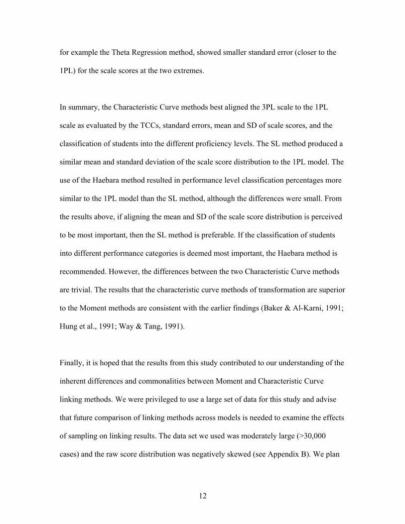
metric. The scale score mean and SD are shown in Table 1 and plotted in Figures 5 and 6,

respectively. The results showed that the scale score mean from the SL method (676.7) is

closer to the 1PL model mean (681.9) than the mean from any of the other methods. The

scale score means produced by all other methods are smaller than the SL method, as

follows: Haebara (675.7), Theta Regression (652.2), Mean/Mean (635.0), and

Mean/Sigma (628.5).

The standard deviation (SD) of the scale score distribution that resulted from the use of

the Mean/Sigma method (78.5) is closest to the 1PL model SD (80.3), followed by the

SDs of the SL (88.3), Haebara (90.3), and Theta Regression (93.3) methods. The

Mean/Mean method produced a comparatively large SD (122.2). Note that both the scale

score mean and SD are smallest for the Mean/Sigma method.

Cumulative frequency distributions are plotted in Figure 7. The proportion of students

obtaining a given scale score is very similar for the 1PL, SL, and Haebara methods. The

cumulative frequency distribution curves for SL and Haebara are virtually

indistinguishable. The Mean/Mean, Mean/Sigma, and Theta Regression methods resulted

in lower scale scores than the 1PL, SL, and Haebara methods throughout most of the

9

ability range. Note that due to the assumptions in the 1PL model that disallow for

guessing to be modeled, the scale score corresponding to the first percentile is higher for

the 1PL method, than any of the others.

It is evident from the results above that the SL and Haebara methods provided a more

accurate link to the 1PL scale than the Mean/Mean, Mean/Sigma, and Theta Regression

methods.

Proficiency Level Classification

The impact of the linking methods on the classification of students into the different

performance level categories is shown in Table 2. As is evident from the cumulative

distribution function, the SL and Haebara methods classified similar proportions of

students into the Unsatisfactory, Limited Knowledge, Satisfactory, and Advanced

categories as the 1PL model. Both of the SL and Haebara methods classified 32.1%

students at or above the Satisfactory category, which is very similar to the classification

by the 1PL model (1PL classified 33.4% students at or above the Satisfactory category).

Looking at the Satisfactory and Advanced levels separately, the Characteristic Curve

methods’ classification percentages (Haebara: Satisfactory = 23.7%, Advanced = 8.4%;

SL: Satisfactory = 24.1%, Advanced = 8.0%) are close to those of the 1PL method

(Satisfactory = 23.1%, Advanced = 10.3%). The classification percentages of the Haebara

method align best with those of the 1PL method. The Moment (Mean/Mean and

Mean/Sigma) and Theta Regression methods classified more students in the

Unsatisfactory category and fewer students at or above the Satisfactory category. The

10

Mean/Mean method placed fewer students in the Limited Knowledge category, and the

Mean/Sigma method placed more students in the Unsatisfactory category, than any other

method.

Summary and Discussion

This study evaluated the use of several equating methods to link 3PL parameter estimates

to a 1PL scale in order to identify empirical evidences depicting the effects of different

equating/linking techniques when the linking administration was calibrated under a

different IRT model than the model for the current administration. The results indicated

that, except for test information, the SL and Haebara methods of linking to the 1PL scale

showed results most similar to the 1PL model. The difference at the lower asymptote in

the SL and Haebara methods’ TCCs and the 1PL method TCC is characterized by the

difference between the 3PL and 1PL models in modeling guessing. The Moment and

Theta Regression methods estimated a higher proportion of students in the lower ability

range.

Since the standard error of the scale scores produced by the Mean/Sigma method is

smallest in the middle of the scale score distribution, and the SL and Haebara methods

resulted in the smallest standard error at slightly above the middle of the distribution (see

Figure 2), the information provided by these methods are also higher at the given scale

score range (see Figure 4). The standard errors of Moment and Theta Regression methods

are comparatively larger in the middle of the scale score range. Some of these methods,

11

for example the Theta Regression method, showed smaller standard error (closer to the

1PL) for the scale scores at the two extremes.

In summary, the Characteristic Curve methods best aligned the 3PL scale to the 1PL

scale as evaluated by the TCCs, standard errors, mean and SD of scale scores, and the

classification of students into the different proficiency levels. The SL method produced a

similar mean and standard deviation of the scale score distribution to the 1PL model. The

use of the Haebara method resulted in performance level classification percentages more

similar to the 1PL model than the SL method, although the differences were small. From

the results above, if aligning the mean and SD of the scale score distribution is perceived

to be most important, then the SL method is preferable. If the classification of students

into different performance categories is deemed most important, the Haebara method is

recommended. However, the differences between the two Characteristic Curve methods

are trivial. The results that the characteristic curve methods of transformation are superior

to the Moment methods are consistent with the earlier findings (Baker & Al-Karni, 1991;

Hung et al., 1991; Way & Tang, 1991).

Finally, it is hoped that the results from this study contributed to our understanding of the

inherent differences and commonalities between Moment and Characteristic Curve

linking methods. We were privileged to use a large set of data for this study and advise

that future comparison of linking methods across models is needed to examine the effects

of sampling on linking results. The data set we used was moderately large (>30,000

cases) and the raw score distribution was negatively skewed (see Appendix B). We plan

12

to further investigate the impact of these methods on score distribution when the sample

size is smaller and/or with various sample raw score distributions, for example normal,

bimodal, etc.

13

References

Baker, F. B., & Al-Karni, A. (1991). A comparison of two procedures for computing IRT

equating coefficients. Journal of Educational Measurement, 28, 147-162. Bock, R. D. (1972). Estimating item parameters and latent ability when responses are

scored in two or more nominal categories. Psychometrika, 46, 443-459. Burket, G. (2002). PARDUX [Computer program]. Unpublished. Monterey, CA: CTB

McGraw-Hill. Divgi, D. R. (1986). Does the Rasch model really work for multiple choice items? Not if

you look closely. Journal of Educational Measurement, 23, 283-298. Haebara, T. (1980). Equating logistic ability scales by a weighted least squares method.

Japanese Psychological Research, 22, 144-149. Hanson, B. and Zeng, L. (1995). ST [A computer program for IRT scale transformation,

Version 1.0]. Unpublished, American College Testing. Hung, P., Wu, Y., & Chen, Y. (1991). IRT item parameter linking: Relevant issues for the

purpose of item banking. Paper presented at the International Academic Symposium on psychological Measurement, Tainan, Taiwan.

Kolen, M. J., & Brennan, R. L. (1995). Test equating: methods and practices. Springer-

Verlag New York, Inc. Lord, F. M. (1980). Applications of item response theory to practical testing problems.

Hillsdale, NJ: Lawrence Erlbaum Associates. Loyd, B. H., & Hoover, H. D. (1980). Vertical equating using the Rasch model. Journal

of Educational Measurement, 17, 179-193. Marco, G. L. (1977). Item characteristic curve solutions to three intractable testing

problems. Journal of Educational Measurement, 14, 139-160. Muraki, E. (1992). A generalized partial credit model: Application of an EM algorithm.

Applied Psychological Measurement, 16, 159-176. Rasch, G (1960). Probabilistic models for some intelligence and attainment tests.

Copenhagen: Danish Institute for Educational Research. Stocking, M, L., & Lord, F. M. (1983). Developing a common metric in item response

theory. Applied Psychological Measurement, 7, 201-210.

14

Traub, R. E. (1983). A priori considerations in choosing an item response model. In R. K. Hambleton (Ed.), Applications of item response theory (pp. 57-70). Vancouver, BC: Educational Research Institute of British Columbia.

Yen, W. M. (1993). Scaling performance assessments: Strategies for managing local item

dependence. Journal of Educational Measurement, 30, 187-213. Way, W. D., & Tang, K. L. (1991). A comparison of four logistic model equating

methods. Paper presented at the annual meeting of the American Educational Research Association, Chicago.

15

Table 1. Scaling Constants and Scale Score Descriptive Statistics Scaling Constants to

Place 3PL Item Parameters onto

1PL scale

Final Scaling Constants

(M1’=M1*75, M2’=M1*M2+680)

Scale Score Descriptive Statistics

Methods M1 M2 M1’ M2’ Mean SD 1PL 1.0 0.0 75.0 680.0 681.9 80.3 Mean/Mean 1.4 -0.4 107.5 652.2 635.0 122.2 Mean/Sigma 0.9 -0.5 65.6 640.0 628.5 78.5 Regression 1.1 -0.2 79.1 665.7 652.2 93.3 SL 1.0 0.1 73.8 689.6 676.7 88.3 Haebara 1.0 0.1 75.8 688.9 675.7 90.3

Table 2. Performance Level Classification, N=31,813

Methods Unsatisfactory Limited

Knowledge Satisfactory Advanced 1PL 39.7% 26.9% 23.1% 10.3% Mean/Mean 55.5% 20.2% 15.3% 9.1% Mean/Sigma 63.9% 26.1% 8.6% 1.3% Regression 49.9% 27.5% 17.1% 5.5% SL 37.7% 30.1% 24.1% 8.0% Haebara 38.4% 29.5% 23.7% 8.4%

16

Figure 1. Test Characteristic Curves

Figure 2. Standard Error Curves

17

-Mean/Mean -Mean/Sigma -Theta Regression-SL -Haebara -1PL

-Mean/Mean -Mean/Sigma -Theta Regression-SL -Haebara -1PL

Figure 3. Frequency Distribution Curves

Figure 4. Test Information Functions

18

-Mean/Mean -Mean/Sigma -Theta Regression-SL -Haebara -1PL

-Mean/Mean -Mean/Sigma -Theta Regression-SL -Haebara -1PL

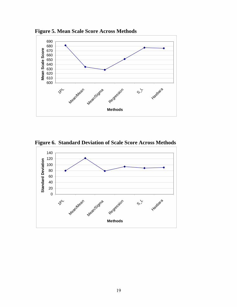
Figure 5. Mean Scale Score Across Methods

600610620630640650660670680690

1PL

Mean/M

ean

Mean/Sigm

a

Regress

ionS_L

Haebara

Methods

Mea

n S

cale

Sco

re

Figure 6. Standard Deviation of Scale Score Across Methods

020406080

100120140

1PL

Mean/M

ean

Mean/Sigm

a

Regress

ionS_L

Haebara

Methods

Sta

ndar

d D

evia

tion

19

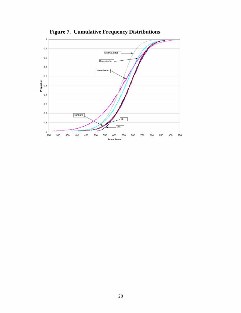
Figure 7. Cumulative Frequency Distributions

0

0.1

0.2

0.3

0.4

0.5

0.6

0.7

0.8

0.9

1

250 300 350 400 450 500 550 600 650 700 750 800 850 900 950

Scale Score

Prop

ortio

n

Mean/Sigma

Regression

Mean/Mean

1PL

SL

Haebara

20

Appendix A. Comparison of Standard Errors

-1PL-Mean/Mean

-1PL-Mean/Sigma

-1PL-Theta Regression

-1PL-S_L

-1PL-Haebara

21

Appendix B. Raw Score Frequency Distribution

0

100

200

300

400

500

600

700

800

900

1000

5 7 9 11 13 15 17 19 21 23 25 27 29 31 33 35 37 39 41 43 45 47 49 51 53 55 57 59 61 63 65 67 69 71 73 75 77

Raw Score

Freq

uenc

y

22