evaluation of lens distortion errors using an underwater ... · evaluation of lens distortion...
TRANSCRIPT

NASA Technical Memorandum 104795
Evaluation of Lens Distortion ErrorsUsing an Underwater Camera Systemfor Video-Based Motion Analysis
Jeffrey PolinerLockheed Engineering & Sciences CompanyHouston, Texas
Lauren FletcherGlenn K. Klute
Lyndon B. Johnson Space CenterHouston, Texas
National Aeronautics and
Space Administration
https://ntrs.nasa.gov/search.jsp?R=19940029451 2020-05-12T17:14:47+00:00Z

ACKNOWLEDGMENTS
This study, supported by the National Aeronautics and Space Administration
under contract number NAS9-18800, was conducted in the Anthropometry
and Biomechanics Laboratory and the Weightless Environment Training
Facility at the Johnson Space Center in Houston, Texas. The authors would
like to thank Lara Stoycos for her assistance in conducting the study as well as
for her review of the manuscript. We would also like to thank Sudhakar
Rajulu and Robert Wilmington for their review and comments on the
manuscript.

CONTENTS
Section Page
INTRODUCTION ................ . ........................................................................................... 1
METHODS ....................................................................................................................... 3
Data Collection ................................................................................................. 3
Data Analysis .................................................................................................... 4
RESULTS ......................................................................................................................... 5
DISCUSSION ................................................................................................................... 14
CONCLUSIONS ............................................................................................................... 15
REFERENCES ................................................................................................................... 16
iii

Figure
1.
2.
3.
4.
5.
6.
HGURES
Page
Barrel distortion from a video lens ................................................................... 2
Grid of lines used in the study ............................................................................ 4
Calculated normalized coordinates of points .................................................. 6
Error contour plots for each of the four trials .................................................. 9
Error as a function of radial distance from center of the image .................. 11
Average error as a function of radial distance for combined data .............. 14
TABLES
Table Page
1. Descriptions of the Various Trials ..................................................................... 3
2. Coefficients of Linear and Binomial Regressions ........................................... 13
iv

INTRODUCTION
Video-based motion analysis systems are widely employed to study human
movement, using computers to capture, process, and analyze video data.
This video data can be collected in any environment where cameras can belocated.
The Anthropometry and Biomechanics Laboratory (ABL) at the Johnson
Space Center is responsible for the collection and quantitative evaluation of
human performance data for the National Aeronautics and Space
Administration (NASA). One of the NASA facilities where human
performance research is conducted is the Weightless Environment Training
Facility (WETF). In this underwater facility, suited or unsuited crewmembers
or subjects can be made neutrally buoyant by adding weights or bouyant foam
at various locations on their bodies. Because it is underwater, the WETF
poses unique problems for collecting video data. Primarily, cameras must be
either waterproof or encased in a waterproof housing.
The video system currently used by the ABL is manufactured by Underwater
Video Vault. This system consists of closed circuit video cameras (Panasonic
WV-BL202) enclosed in a cylindrical case with a plexiglass dome covering the
lens. The dome used to counter the magnifying effect of the water is
hypothesized to introduce distortion errors.
As with any data acquisition system, it is important for users to determine the
accuracy and reliability of the system. Motion analysis systems have many
possible sources of error inherent in the hardware, such as the resolution of
recording, viewing and digitizing equipment, and lens imperfections and
distortions. Software errors include those caused by rounding and
interpolation. In addition, there are errors which are introduced by the use of
the system, such as inaccurate or incomplete calibration information,
placement of cameras relative to the motions being investigated, and
placement of markers at points of interest. Other errors include obscured
points of interest and limited video sampling rates.
Image distortions will introduce errors into any analysis performed with a
video-based motion analysis system. It is, therefore, of interest to determine
the degree of this error in various regions of the lens. A previous study
(Poliner, et al., 1993) developed a methodology for evaluating errors
introduced by lens distortion. In that study, it was seen that errors near the
center of the video image were relatively small and the error magnitude
increased with the radial distance from the center. Both wide angle and
standard lenses introduced some degree of barrel distortion (fig. 1).
1

Figure 1. Barrel distortion from a video lens. Top: original image. Bottom: distorted image.
Since the ABL conducts underwater experiments that involve evaluating
crewmembers' movements to understand and quantify the way they will
perform in space, it is of interest to apply this methodology to the camerasused to record underwater activities. In addition to distortions from the lens
itself, there will be additional distortions caused by the refractive properties ofthe interfaces between the water and camera lens.
This project evaluates the error caused by the lens distortion of the cameras
used by the ABL in the WETF.
2

METHODS
Data Collection
A grid was constructed from a sheet of 0.32 cm (0.125 in) Plexiglas. Thin black
lines spaced 3.8 cm (1.5 in) apart were drawn vertically and horizontally on
one side of the sheet. Both sides of the sheet were then painted with a WETF
approved white placite to give color contrast to the lines. The total grid size
was 99.1 x 68.6 cm (39.0 x 27.0 in). The intersections of the 19 horizontal and
27 vertical lines defined a total of 513 points (fig. 2). The center point of the
grid was marked for easy reference. Using Velcro, the grid was attached to a
wooden frame, which was then attached to a stand and placed on the floor of
the WETF pool.
At the heart of the Video Vault system was a Panasonic model WV-BL202
closed circuit video camera. The camera had been focused above water,
according to the procedures described in the Video Vault users manual,
attached to a stand, and placed on the WETF floor facing the grid. Divers used
voice cues from the test director for fine alignment of the camera with the
center of the grid. By viewing the video on poolside monitors, the camera
was positioned so that a predetermined region of the grid nearly filled the
field of view. The distance from the camera to the grid was adjusted several
times, ranging from 65.3 to 72.6 cm (25.7 to 28.6 in). Data collection consisted
of videotaping the grid for at least 30 seconds in each of the positions, with
each position considered a separate trial. Descriptions of the arrangements of
the four trials are given in table 1. Distance refers to the distance from the
camera to the grid. Image size was calculated by estimating the total number
of grid units from the video. The distance from the outermost visible grid
lines to the edge of the image was estimated to the nearest one-tenth of a grid
unit. The distance and image size values are all in centimeters.
Table 1. Descriptions of the Various Trials
TRIAL DISTANCE
1 72.62 66.03 65.34 65.3
IMAGE SIZE
x Y
80.4 61.773.5 55.672.4 54.972.4 55.3
GRID LINES
x Y
21 17
19 1519 1519 14
#
POINTS
357285285266
3

3.8r! I
r
II,3.8 cm
99.1 cm
b_o3
Figure 2. Grid of lines used in the study. Intersections of lines were used as test points.
Data Analysis
An Ariel performance analysis system (APAS) was used to process the video
data. Recorded images of the grid were played back on a VCR. A personal
computer was used to grab and store the images on disk. For each trial,several frames were chosen from the recording and saved, as per APAS
requirements. From these, analyses were performed on a single frame foreach trial.
Because of the large number of points (up to 357) being digitized in each trial
and the 32-point limitation of the APAS system (software rev. 6.30), the grid
was subdivided into separate regions for digitizing and analysis. Each row
was defined as a region and digitized separately.
An experienced operator digitized all points in the grid for each of the trials.
Here digitizing refers to the process of the operator identifying the location of
points of interest in the image with the use of a mouse-driven cursor. Often
digitizing is used to refer to the process of grabbing an image from videoformat and saving it in digital format on the computer. Digitizing and
subsequent processing resulted in X and Y coordinates for the points.
4

Part of the digitizing process involved identifying points of known
coordinates as control (calibration) points. Digitization of these allows for
calculation of the transformation relations from image space to actual
coordinates. In this study, the four points diagonal from the center of the grid
were used as the control points (points marked "X" in fig. 2). These were
chosen because it was anticipated that errors would be smallest near the
center of the image. Using control points which were in the distorted region
of the image would have further complicated the results. The control points
were digitized and their known coordinates were used to determine the
scaling from screen units to actual coordinates.
For trial 1, the coordinates ranged from 0 to approximately +38.1 cm in the X
direction and 0 to approximately +30.48 cm in the Y direction. For trials 2 and
3, the ranges were 0 to +34.29 cm in X and 0 to +_26.67 cm in Y. For trial 4, the
range was 0 to +_34.29 cm in X and 0 to -22.86 and +26.67 in Y. To remove the
dependence of the data on the size of the grid, normalized coordinates were
calculated by dividing the calculated X and Y coordinates by half the total
image size in the X and Y directions, respectively. Table 1 lists these sizes forthe four trials. Thus, normalized coordinates in both the X and Y directions
were dimensionless and ranged approximately from -1 to +1 for all four trials.
For all trials, the error for each digitized point was calculated as the distance
from the known coordinates of the point to the calculated coordinates.
RESULTS
Raw data from the four trials are presented in figure 3. Shown are graphs of
the calculated normalized coordinates of points. Grid lines on the graphs do
not necessarily correspond to the grid lines which were videotaped. Note the
slight barrel distortion evident especially near the edges of the images.
5

Trial 1
I
t +-t .4-+ "1"'1"4-'1" I-.44 4-4 4-1-++ 4-+-4 .4-4--t .1.++.1. 4-.1. I-+- .1.-4 .1..1.+.1. 4-4-_ .L
+-t,+++4 t-+ -.4-4 .1.-4 "1".1..4..1. -.1. ,.4-
i "' ; ; ,_ 1, .2 '. ', ', .. '. ', ; 1'4--4- t
+-_ .1.++-1- F .4- I-+- .1.-4 +++4++ -t-
.4._.4 +t_ h t -t- -P_ .4-+++++ .4,
+-;.4+++ _-4 -.1.- .1.4 .4..1.+.4.++ +
+-_.4+++ _--t- --4-- -4-" +-t-+-t-+-I- ,+N
...._
0 -L-L J- J- .L.J- L -L -L -L., _I_.,L _L -L.L-,L -L................... - .
-t-+ .4..1. _-.1. t- 4- - .1. - .4- _ 4-1- +.1. ++ ,+
Zo-0.2. _r+4.4 _-+ _.1. -+- +4 .1..4..1..1.++ +
•4"++.1.+.4, I-4 -+- .1.-4 ++-4-+++ +
++.4..1.++ I-4 -.4-4 .1.-4 .4-.4-.4-4-++.4- +
4-+ : + t ; "' ; -r_ _-1 +÷'_; i I '. "J-
++.4..1.++ I-4 -.+4 .1.-4 .4-.4-.4-+4-.4- ,-t-
"h-_-h4+4 I--t- --4-4 4-14+++'h-r ,4.
+Jr+++.4 F 4 -.4-4 4-t 44++ 4- -t- '+-1
-1 -0.8-0.6-0.4-0.2 0 0.2 0.4 0.6 0.8
No_nalized X
_o-0.2.Z
Trial 2
-1
+ +.+++I I '. ; _ ', -i'4-r -t-
+ .4-_ -4-- +- + 4 -4-- +, .1. ..1.1.4+
+- .4-4 .4-- +- .1. _ .1. -+ .4- +-4-4-
' ' 4"' .LJ --.. , _ , " 4"
+- "1"-4"1"_ +- .4-* "1" "'1" "1" "+'_ "1"
+_, +÷ + _ +_ +" + i + + +4 +..1. .._-I. J- .J. -L J .I- -L .JL -L -L_
+ +
•1..1.-4.1..4..1.- .1.L.4..4-.1.-4+! 1 l • I , i I J.
+_ 4- +- +-4 .4.-t 4- +- +' .1.+.4.
+-t +4 + - +-4 4 - .1.- .4._ + .4-_ 4
.,_ 1 l • • 1 ¢ ...... , l I ..I
i * • • l I l '
I +-4 .1.4 + _ .4--4.4,_ .1.- +_ .4-.1.4"4"
-1 -0.8 -0.6 -0.4-0.2 0 0.2 0.4 0.6 0.8 1
Normalized X
Figure 3. Calculated normalized coordinates of points.

0.(
>,
_0
0
oZ
Trial 3
+ 4 +4 +- + A + 4 +
"W ' l | ! It , • , ,
+4+" +'_ +4 ++4
+4 +4 +- +'] + 4 +
: .+ + 4-4 4-4-4 4-4--_ 4-
+_ +4+- +q + +
+4 +++q +q + +
4- ._ 4- -g 4-.4 ..t..a ..t. -L
++ ++ +'+ +4 + +
+'t ++ +-_ +4 + +
• ,t , , • , r n
+4 +4 +-t +4 + +
+4 +4 +-t + + +- +
t | ..........
, ! l I =?-
+'_ + +q +
+ -+ +ff +
+ -+ +ff +
+ -+ +q +
+ + -+- +
-L. -L. _ -I- .I -I-
+ _+ -+ F+
+- + +-_ +
', ,. ,,
+ _ + -+_ +
+4 + +" +
; ', , +
+'_ +- +-_ +4 +- +- +_ + ++ +
-1 -0.8-0.6-0.4-0.2 0 0.2 0.4 0.6 0.8
Normalized X
0
oZ
-1
Trial 4
,,i, _.+_.+-_. +-+.. +
+4 +4 +.4 +_ +
+-t +- +-_ +-t +
+ 4.+4. _ ,. ', ',.
!+ ++ ++ "+ +4 +
+4 +4 +-t +4 +
•k-_,+-J, _ ,. ', ,. '. .. ',
/+ ++ +- +'_ +'_ +4 +_+-I-++ +
/
+- +- +- +4 4 +4 +++
+-_+- +- +4 + + "+- +4 +++
.t__ --_ .a.. 4- .4 4- .x.. _t_ _ + ,, _ ,, [
+q +- + 4 +4 + - + + +- +-t+
+-_ +-_ + 4 +4 + + _ + t + +-_ +
I1+ + + -+_ +
+++I , ,. .s.---
+ -+ s+ F+ h+
+ + +- +-t+
,. .._ _4 4-
-1 -0.8-0.6-0.4-0.2 0 0.2 0.4 0.6 0.8
Normalized X
Figure 3. (concluded.)
7

For each trial, the error of each point was calculated as the distance between
the calculated location (un-normalized) and the known location of that point.
These error values were then normalized by calculating them as a percent of
half the image size in the horizontal direction (trial L 40.2 Cm; trial 2, 36.8 cm;
trials 3 and 4, 36.2 cm). This dimension was chosen arbitrarily to be
representative of the size of the image.
Figure 4 presents contour plots of the normalized error as a function of the
normalized X-Y location in the image for each of the trials. This type of
graph, commonly used in land elevation maps, displays information three-
dimensionally. The coordinate axes represent two of the dimensions. Here,
these were the X and Y coordinates of the points. The third dimension
represents the value of interest as a function of the first two dimensions, in
this case, the error as a function of the X and Y location. Curves were created
by connecting points of identical value.
Interpreting these graphs is similar to interpreting a land map; peaks and
valleys are displayed as closed contour lines. Once again, it was clear that
errors were small near the center of the image and became progressively
greater further away from the center.
The unevenness evident in some of these graphs can be partly attributed to
splitting the image into separate regions for the purpose of digitizing. The
control points were redigitized for each individual section. Since the control
points were close to the center of the image, a small error in their digitization
would be magnified for points further away from the center.
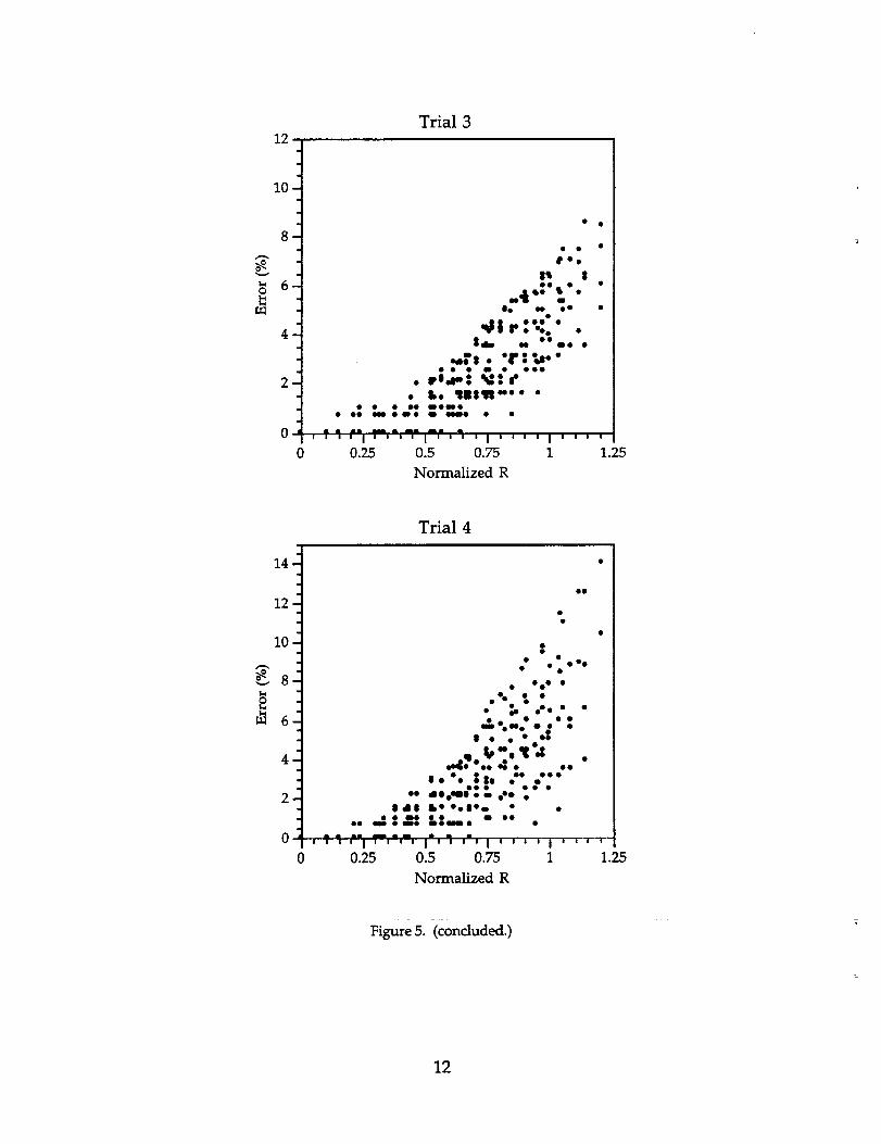
Another quantitative way of viewing this data was to examine how the error
varied as a function of the radial distance from the center of the image. This
distance was normalized by dividing by half the image size in the horizontal
direction (trial 1, 40.2 cm; trial 2, 36.8 cm; trials 3 and 4, 36.2 cm). Figure 5
presents these data for each of the four trials.
8

Trial 1
.*'4
o3
z
-1 -0.8-0.6-0.4-0.2 0 0.2 0.4 0.6 0.8 1
Normalized X
0.8--
0.6-
0.4-
0.2-
_ -0.2-
-0.4-
-0.6-
-0.8-
-1
Trial 2
I I I I I I I
-0.8-0.6-0.4-0.2 0 0.2 0.4 0.6 0.8 1
Normalized X
Figure 4. Error contour plots for each of the four trials. All coordinates have been normalized.
9

Trial 3
0.8
0.6
0.4
>-
_-0.2
Z
-0.4
-0.6
i I I I I-1 -0.8-0.6-0.4-0.2 0 0.2 0.4 0.6 0.8 1
Normalized X
Trial 41
080.6-
0.4- 4
0.2-
i°-_ -0.2-
-0.4- _
-0.6- < 3;,
-0.8-
-1 I I I I I I I I I- -0.8-0.6-0.4-0.2 0 0.2 0.4 0.6 0.8 1
Normalized X
Figure 4. (concluded.)
10

12Trial 1
10
8
6
%
0
°o °
oo
0_ 00
• eJ • oeO• 05 q,e0 •
• 0 • 0o0 •• qP• Ore- •
otK o• FO
_ t_,t,sml, •• • • • 0• • 00•
• CoOl'•@ _o •o • %8•5188W u518• •
• o • J|"o°Som|_ •
_""a_'a':'"n ' ' ' ' J .... u ....0.25 0.5 0.75 1 1.25
Normalized R
12Trial 2
10
.
0
0
80_ • e• °
•eOo _o •eO• • • •qo8. tt •
. "t- .a • ..• "..._ LU "
---',;:4;'r: "o• Lo°•14°8 • o•
• 0o •oo,_o•o• •• • •0 Ira@ • mO • • •OO • O • •
" I ' ' ' ' I _" ' I ' ' ' ' I ' ' ' '
0.25 0.5 0.75 1 1.25
Normalized R
Figure 5. Error as a function of radial distance (R) from the center of the image for four trials.All coordinates have been normalized.
11
12
Trial 3
10
v
6o
g • •
It $ •
oe4 q,o°• _• •
+;;:-.:. •°o o •
Sdl e• •• co• •
_.r:. "r:_.-• • • No • ••0
• pod-: _:: _"• k' '1815'1"'" "
• • • 00 8o00o•
• 00 _ • (m • Ib 4Joll41J • •
i m i8' ?_ "'i .... I ;'" ' l .... I ....
0.25 0.5 0.75 1 1.25
Normalized R
Trial 4
14-
12
10-
g8o
m 6
4-
2-
0-
0
--:.: . ." :
I •,.0"_|,, ;p o';o..;. ".. -8 • ..
0.'. :l. " ""Ill •• •
00 dO•eoe •ee 0"o •Id$ L ° °olOo • •
00 --;=.."0 -;..00 - 00 .
"r ;'I " "i ? _",',', i ,_ , , I , I , , I , , , ,0.25 0.5 0.75 1 1.Z5
Normalized R
Figure 5. (concluded.)
12

Linear and binomial regressions were then fit to the data for each trial and forall data combined. The linear fit was of the form
Error = Ao + A1 R
where R was the radial distance from the center of the image (normalized),
and A0 and A1 were the coefficients of the least-squares fit. The binomial fitwas of the form:
Error = Bo + B1 R + B2 R 2
where Bo, B1, and B2 were the coefficients of the fit. The results of these least-
squares fits are presented in table 2. The columns labeled "RC" are the
squares of the statistical regression coefficients (r2).
Table 2. Coefficients of Linear and Binomial Regressions
LINEAR FIT BINOMIAL FIT
Trij_Jl A0 A_j.1 RC1 B0 B._].I B2 RC2
1 -1.985 6.592 0.735 0.1257 -1.104 5.878 0.7872 -1.828 5.819 0.657 0.3773 -2.395 6.403 0.7203 -1.852 6.285 0.698 0.0698 -0.760 5.406 0.7444 -2.410 8.229 0.604 0.3035 -1.928 7.935 0.651
combined -2.000 6.679 0.636 0.1980 -1.434 6.264 0.684
Figure 6 presents the binomial regression for the error as a function of radialdistance for all the data combined.
13

9
0 ' ! ' I ' I ' i '0 0.25 0.5 0.75 1 1.25
Normalized R
Figure 6. Average error as a function of radial distance (R) from the center of the screen for datacombined from all four trials. All coordinates have been normalized.
DISCUSSION
When reviewing these results, several points should be noted. First, this
study utilized a two-dimensional analysis algorithm. A limitation of the
APAS system (rev. 6.30) was that exactly four calibration points were required
to define the scaling from screen coordinates to actual coordinates. The use of
more than four points would likely result in less variability. Second, allcoordinates and calculated errors were normalized to dimensions of the
image. Although there were many possibilities for the choice of dimension
(e.g., horizontal, vertical or diagonal image size; maximum horizontal,
vertical, or diagonal coordinate; average of horizontal and vertical image size
or maximum coordinate; etc.), the dimensions used to normalize were
assumed to best represent the image size.
It is clear from these data that a systematic error caused by lens distortion
occurred when using the underwater video system. Lens distortion errors
were less than 1% from the center of the image up to radial distances
equivalent to 25% of the horizontal image length (normalized R equal to 0.5).
Errors were less than 5% for normalized R up to 1, an area covering most of
the image. Errors in the comers due to lens distortion were approximately
8%. Note that this accuracy relates only to lens distortion. There are many
other sources of error (lens imperfections, incomplete calibration point
information, digitizing resolution, etc.) which could add to these values.
14

There seemed to be some degree of random noise. This was evident in the
scatter pattern seen in the graphs in figure 5. This error can most likely be
attributed to the process of digitizing. There are factors which limit the ability
to correctly digitize the location of a point, such as: if the point is more than
one pixel in either or both dimensions, irregularly shaped points, a blurred
image, shadows, etc. Because of these factors, positioning the cursor when
digitizing was often a subjective decision. It should be pointed out that the
error caused by this subjective method of identifying points would be reduced
by using a system which automatically identified the centroid of the points of
interest to sub-pixel accuracy.
Four trials were analyzed in this study. Although all the data were
normalized, there were slight differences among the four trials (fig. 5 and
table 2). These can most likely be attributed to the uncertainty in determining
the grid size, which was estimated from the fraction of a grid unit from the
outermost visible grid lines to the edge of the images.
Two types of regressions were fit to the data: linear and binomial. The
interpretation of the coefficients of the linear regression can provide insight
into the data. A 1, the slope of the error-distance relation represents the
sensitivity of the error to the distance from the origin. Thus, it is a measure
of the lens distortion. A 0, the intercept of the linear relation can be
interpreted as the error at a distance of zero. If the relation being modeled
were truly linear, this would be related to the random error not accounted for
by lens distortion. However, in this case, it is not certain if the error-distance
relation was linear. The RC values gave an indication of how good the fit
was. The binomial curve fit seemed to more correctly represent the data. The
interpretation of these coefficients, however, is not as straightforward.
CONCLUSIONS
This study has taken a look at one of the sources of error in video-based
motion analysis using an underwater video system. It was demonstrated that
errors from lens distortion could be as high as 8%. By avoiding the outermost
regions of the lens, the errors can be kept smaller.
REFERENCES
Poliner, J., Wilmington, R.P., Klute, G.K., and Micocci, A. Evaluation of Lens
Distortion for Video-Based Motion Analysis, NASA Technical Paper 3266,
May 1993.
15

Form ApprovedREPORT DOCUMENTATION PAGE OMBNo.O704-O188
Public reporting burden for this collection of information ill estimated to average 1 hour per reeponee, including the time for reviewing inlltructiornl, eearching existing data =ourcell,
gathering end maintaining the data needed, end completing and reviewing the collection of Information. Send comments regarding this burden estimate or any other aspect of thill collection
of information, including suggestions for reducing this burden, to Washington Headqullrterll Services, Directorate for information Operation= end Reports, 1215 Jefferlon Davis Highway,
Suite 1204, Arlington, VA 22202-4302, and to the Office of Mer_gllment and Budget, Paperwork Reduction Project (0704-0198), We=hington, DC 20503.
1. AGENCY USE ONLY (Leave Blank) 2. REPORT DATE 3. REPORT TYPE AND DATES COVEREDJul/94 NASA Reference Publication
4. TITLE AND SUBTITLE
Catalog of Lunar and Mars Science Payloads
6. AUTHOR(S)
Nancy Ann Budden
7. PERFORMING ORGANIZATION NAME(S) AND ADDRESS(ES)
Lyndon B. Johnson Space CenterSolar System Exploration DivisionHouston, Texas 77058
9. SPONSORING/MONITORING AGENCY NAME(S) AND ADDRESS(ESI
National Aeronautics and Space AdministrationWashington, DC 20546
B. FUNDING NUMBERS
8. PERFORMING ORGANIZATIONREPORT NUMBERS
S-777
10. SPONSORING/MONITORINGAGENCY REPORT NUMBER
RP-1345
11. SUPPLEMENTARY NOTES
12a. DISTRIBUTION/AVAILABILITY STATEMENTUnclassified/UnlimitedAvailable from the Center for AeroSpace Information800 Elkridge Landing RoadLinthicum Heights, MD 21090(301) 621-0390 Subject category: 91
12b. DISTRIBUTION CODE
13. ABSTRACT (Maximum 200 wordsJ
This catalog collects and describes science payloads considered for future robotic and human exploration missions to the Moonand Mars. The science disciplines included are geosciences, meteorology, space physics, astronomy and astrophysics, lifesciences, in-situ resource utilization, and robotic science. Science payload data is helpful for mission scientists and engineersdeveloping reference architectures and detailed descriptions of mission organizations. One early step in advanced planning isformulating the science questions for each mission and identifying the instrumentation required to address these questions. Thenext critical element is to establish and quantify the supporting infrastructure required to deliver, emplace, operate, andmaintain the science experiments with human crews or robots. This requires a comprehensive collection of up-to-date sciencepayload information--hence the birth of this catalog.
Divided into lunar and Mars sections, the catalog describes the physical characteristics of science instruments in terms of mass,volume, power and data requirements, mode of deployment and operation, maintenance needs, and technological readiness. Itincludes descriptions of science payloads for specific missions that have been studied in the last two years: the Scout Program,the Artemis Program, the First Lunar Outpost, and the Mars Exploration Program.
14. SUBJECT TERMS
Lunar Exploration, Manned Mars Missions, Instrument Packages, Payloads
17. SECURITY CLASSIFICATION 18. SECURITY CLASSIFICATIONOF REPORT OF THIS PAGE
Unclassified Unclassified
NSN 7540-O1-280-5500
15. NUMBER OF PAGES2]3
16. PRICE CODE
19. SECURITY CLASSIFICAI"]ON 20. LIMITATION OF ABSTRACTOF ABSTRACT
Unclassified UnlimitedStandard Form _;98 (Rev 2-891Prescribed by ANSI Std. 239-18
298-102