evaluation of gvsig and sextante tools for...
TRANSCRIPT

Evaluation of gvSIG and Evaluation of gvSIG and SEXTANTE Tools for SEXTANTE Tools for
Hydrological AnalysisHydrological Analysis
Prof. Dr-Ing Dietrich Schrödera
Mudogah Hildahb and Franz Davidb
Stuttgart University of Applied Stuttgart University of Applied SciencesSciences
1
66thth gvSIG Conference, Valencia, SPAIN gvSIG Conference, Valencia, SPAIN
2
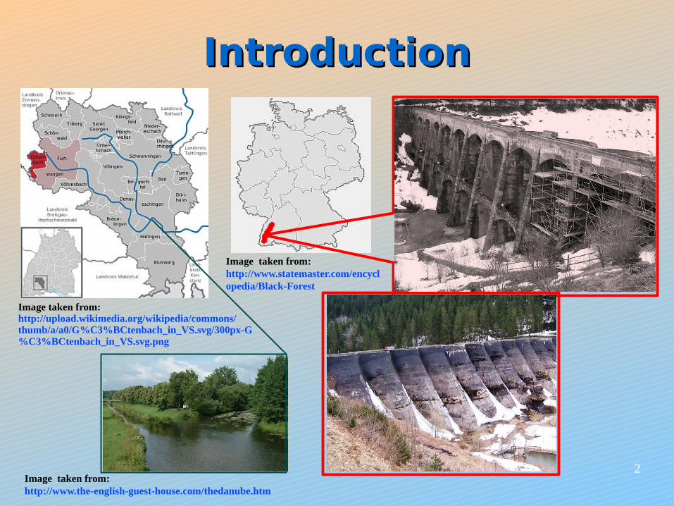
IntroductionIntroduction
Image taken from:http://www.the-english-guest-house.com/thedanube.htm
Image taken from:http://www.statemaster.com/encyclopedia/Black-Forest
Image taken from:http://upload.wikimedia.org/wikipedia/commons/thumb/a/a0/G%C3%BCtenbach_in_VS.svg/300px-G%C3%BCtenbach_in_VS.svg.png
3
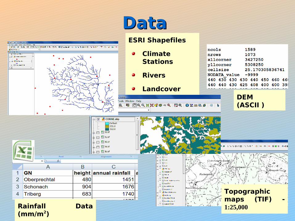
ESRI Shapefiles
Climate Stations
Rivers
Landcover
Data Data
Rainfall Data (mm/m2)
Topographic maps (TIF) - 1:25,000
DEM (ASCII )
4
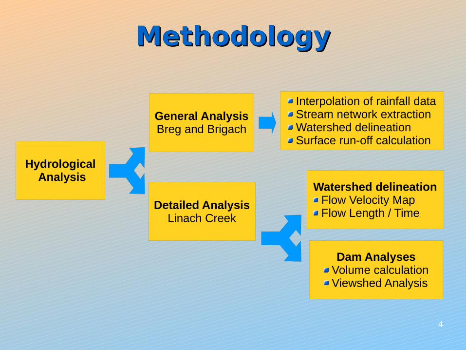
MethodologyMethodologyMethodology
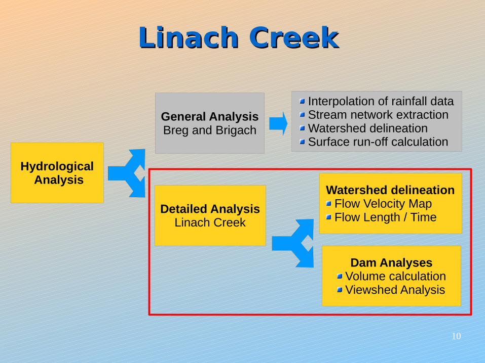
Hydrological Analysis
General AnalysisBreg and Brigach
Detailed AnalysisLinach Creek
Interpolation of rainfall data Stream network extraction Watershed delineation Surface run-off calculation
Watershed delineation Flow Velocity Map Flow Length / Time
Dam Analyses Volume calculation Viewshed Analysis
5
Breg and BrigachBreg and Brigach
Coarse, simplified hydrological modelling of greater region (40 x 55 km2)
Interpolation of the rainfall data
IDW, Nearest Neighbour and Kriging
Stream network extraction
‘Burn-in’ approach
Watershed delineation
Surface run-off calculation
6
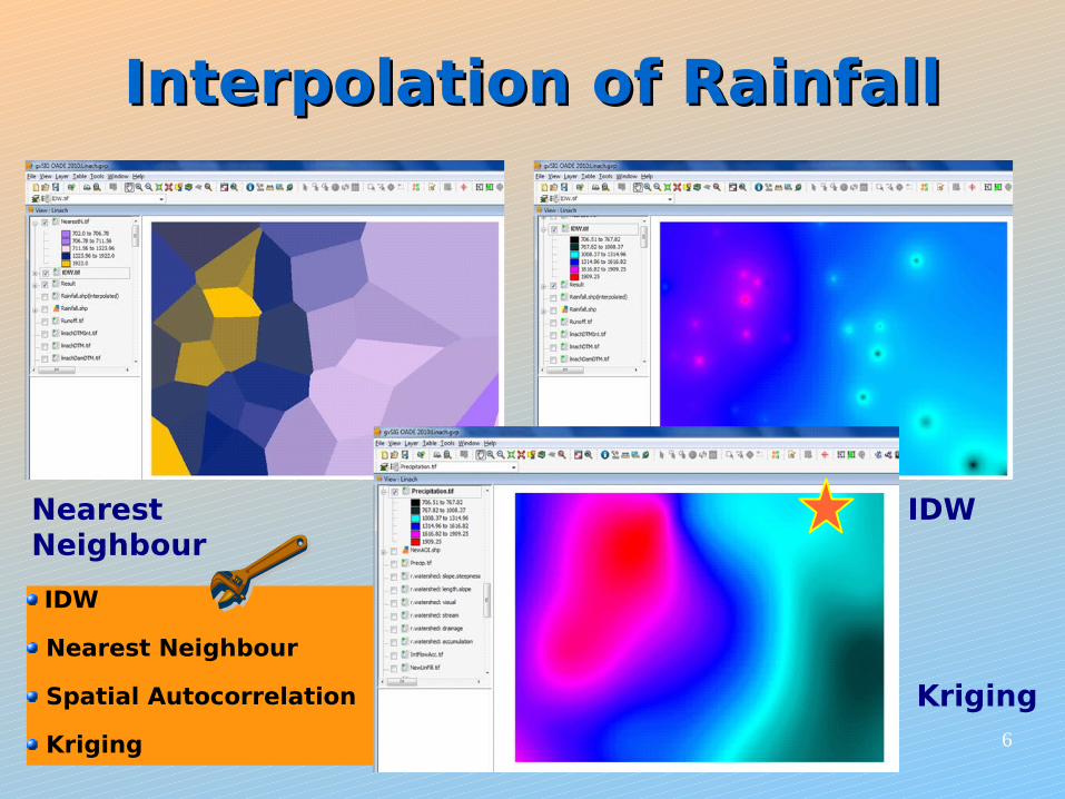
Interpolation of RainfallInterpolation of Rainfall
IDWNearest Neighbour
Kriging
IDW
Nearest Neighbour
Spatial Autocorrelation
Kriging
7
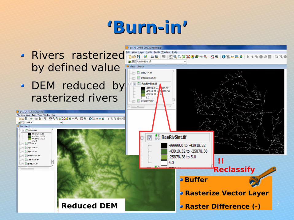
‘‘Burn-in’Burn-in’
Rivers rasterized by defined value
DEM reduced by rasterized rivers
Reduced DEM
!! Reclassify
Buffer
Rasterize Vector Layer
Raster Difference (-)
8
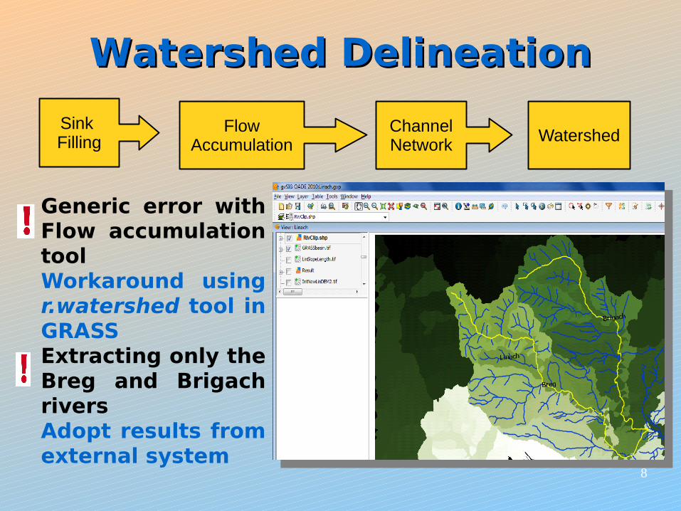
Watershed DelineationWatershed Delineation
Generic error with Flow accumulation toolWorkaround using r.watershed tool in GRASSExtracting only the Breg and Brigach riversAdopt results from external system
Sink Filling
FlowAccumulation
Channel Network Watershed
9
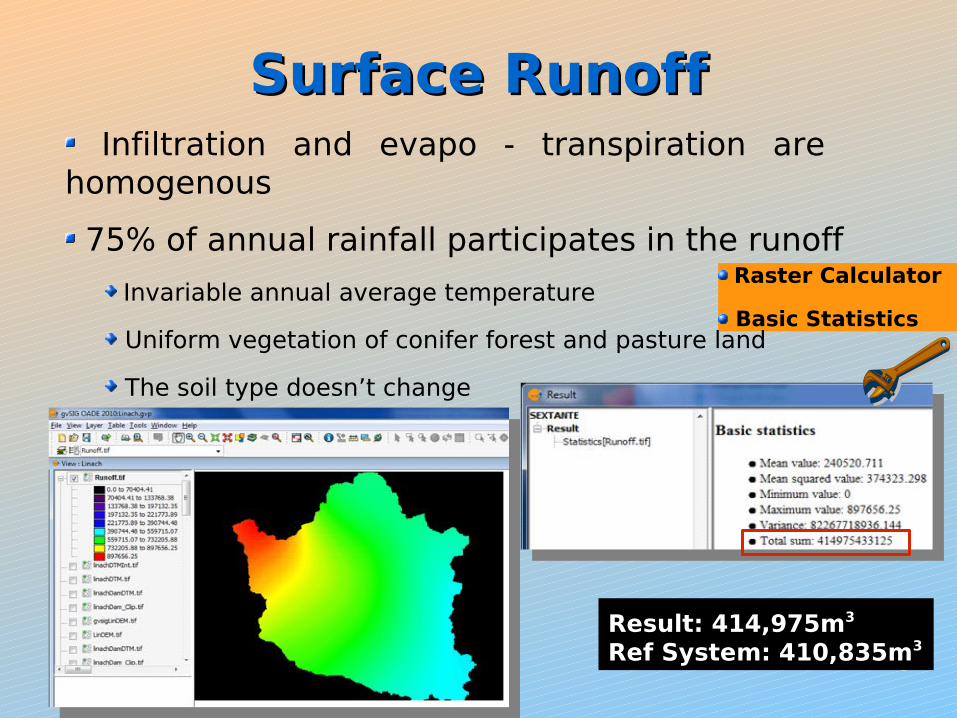
Surface RunoffSurface Runoff Infiltration and evapo - transpiration are homogenous
75% of annual rainfall participates in the runoff Raster Calculator
Basic Statistics
Result: 414,975m3
Ref System: 410,835m3
Invariable annual average temperature
Uniform vegetation of conifer forest and pasture land
The soil type doesn’t change
10
Hydrological Analysis
General AnalysisBreg and Brigach
Detailed AnalysisLinach Creek
Interpolation of rainfall data Stream network extraction Watershed delineation Surface run-off calculation
Watershed delineation Flow Velocity Map Flow Length / Time
Dam Analyses Volume calculation Viewshed Analysis
Linach Creek Linach Creek
11
DEM CreationDEM Creation
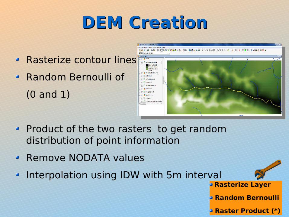
Rasterize contour lines
Random Bernoulli of
(0 and 1)
Product of the two rasters to get random distribution of point information
Remove NODATA values
Interpolation using IDW with 5m interval Rasterize Layer
Random Bernoulli
Raster Product (*)
12
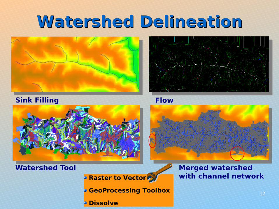
Watershed DelineationWatershed Delineation
Merged watershed with channel network
Watershed Tool
Flow Accumulation
Sink Filling
Raster to Vector
GeoProcessing Toolbox
Dissolve

13
Flow MapsFlow Maps
13
Velocity calculated using Manning Strickler Eq.
Slope
Kst=Resistance Layer
R = Hydraulic RadiusS= Slope raster
Slope Length
Slope
Raster Calculator
Hydrological Length Map
Velocity Map
Resistance Layer
V = KV = Kstst * R * R2/32/3 * S * S1/21/2
14
Flow Time Map & Time-area Flow Time Map & Time-area DiagramDiagram
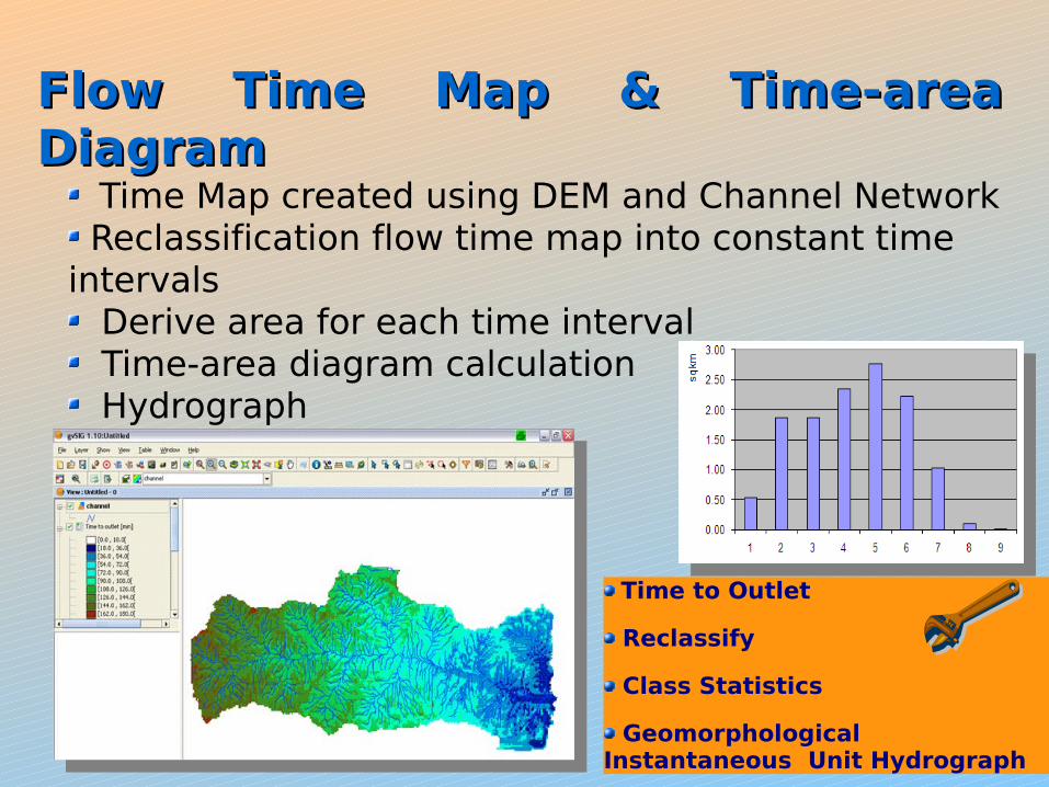
Time Map created using DEM and Channel Network Reclassification flow time map into constant time intervals Derive area for each time interval Time-area diagram calculation Hydrograph
Time to Outlet
Reclassify
Class Statistics
Geomorphological Instantaneous Unit Hydrograph
15
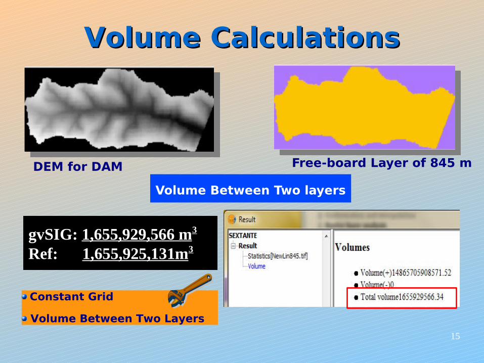
Volume CalculationsVolume Calculations
Volume Between Two layers
gvSIG: 1,655,929,566 m3
Ref: 1,655,925,131m3
DEM for DAM Free-board Layer of 845 m
Constant Grid
Volume Between Two Layers
16
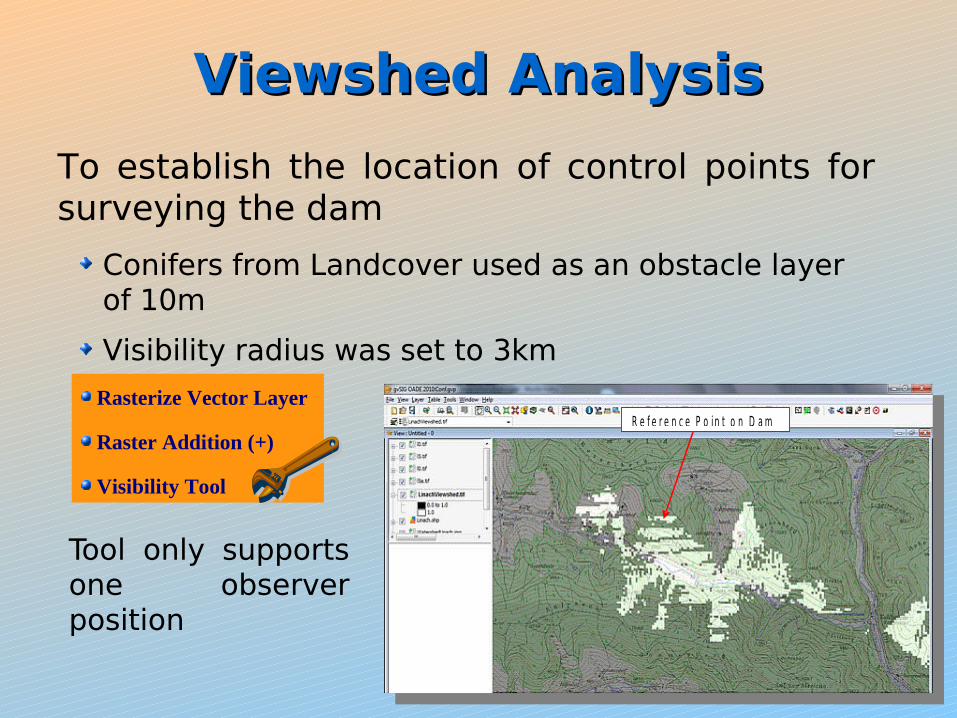
Viewshed AnalysisViewshed Analysis
To establish the location of control points for surveying the dam
Conifers from Landcover used as an obstacle layer of 10m
Visibility radius was set to 3km
Tool only supports one observer position
Rasterize Vector Layer
Raster Addition (+)
Visibility Tool
R e f e r e n c e P o in t o n D a m
17
ChallengesChallenges
Problems with interpretation of NODATA values
NODATA values (often assigned -99,999) used in calculations therefore giving erroneous results
Some tools are too time-consuming
Some tools have an implied size limitation; they don’t run on large datasets but work well on smaller ones
Bugs still exist in some tools
18
ConclusionConclusiongvSIG and SEXTANTE (with GRASS) interface are together very powerful tools
Duplicate tools (GRASS and SEXTANTE) make up for each other
In general:
80% of tools worked well
20% (Error report or Wrong output)
Recommendations
Extend tool documentation (parameter clues, units etc)
Non modal mode for windows would enhance interaction between the tool and map interfaces

19
Thank YouThank You
19