evaluation of corrosion inhibitors - caitcait.rutgers.edu/files/fhwa-nj-2003-005.pdf · evaluation...
TRANSCRIPT
Evaluation of Corrosion Inhibitors
FINAL REPORT
Submitted by Dr. P. N. Balaguru, Principal Investigator
Mohamed Nazier, Graduate Assistant
NJDOT Research Project Manager
Mr. Carey Younger
FHWA NJ 2003-005
In cooperation with
New Jersey Department of Transportation
Division of Research and Technology and
U.S. Department of Transportation Federal Highway Administration
Dept. of Civil & Environmental Engineering Center for Advanced Infrastructure & Transportation (CAIT)
Rutgers, The State University Piscataway, NJ 08854-8014

Disclaimer Statement
"The contents of this report reflect the views of the authors who are responsible for the facts and the
accuracy of the data presented herein. The contents do not necessarily reflect the official views or policies of the New Jersey Department of Transportation or the Federal Highway Administration. This report does not constitute
a standard, specification, or regulation."
The contents of this report reflect the views of the authors, Who are responsible for the facts and the accuracy of the
Information presented herein. This document is disseminated Under the sponsorship of the Department of Transportation, University Transportation Centers Program, in the interest of
information exchange. The U.S. Government assumes no liability for the contents or use thereof.
1. Report No. 2. Government Accession No.
TECHNICAL REPORT STANDARD TITLE PAGE
3. Rec ip ien t ’s Ca ta log No.
5 . Repor t Date
8. Performing Organization Report No.
6. Performing Organizat ion Code
4 . Ti t le and Subt i t le
7 . Author(s)
9. Performing Organization Name and Address 10. Work Unit No.
11. Contracts or Grant No.
13. Type of Report and Period Covered
14. Sponsoring Agency Code
12. Sponsoring Agency Name and Address
15. Supplementary Notes
16. Abstract
17. Key Words
19. Security Classif (of this report)
Form DOT F 1700.7 (8-69)
20. Security Classif. (of this page)
18. Distribution Statement
21. No of Pages 22. Price
December 2002
CAIT/Rutgers
Final Report 02/01/2000 to 09/30/2001
FHWA – NJ-2003-005
New Jersey Department of Transportation CN 600 Trenton, NJ 08625
Federal Highway Administration U.S. Department of Transportation Washington, D.C.
Corrosion of reinforcement is a global problem that has been studied extensively. The use of good quality concrete and corrosion inhibitors seems to be an economical, effective, and logical solution, especially for new structures. A number of laboratory studies are available on the performance of various corrosion inhibiting admixtures. But studies on concrete used in the field are rare. A new bypass constructed by the New Jersey Department of Transportation provided a unique opportunity to evaluate the admixtures in the field. Five new bridge decks were used to evaluate four corrosion-inhibiting admixtures. The primary objective of the study was to evaluate the effectiveness of four commercially available corrosion reduction admixtures. The four admixtures were: DCI-S, XYPEX C-1000, Rheocrete 222+, and Ferrogard 901. The fifth deck was used as a control. All the decks with admixtures had black steel where as the control deck had epoxy coated bars. Extra black steel bars were placed on the control deck. Both laboratory and field tests methods were used to evaluate the admixtures. The uniqueness of the study stems from the use of field concrete, obtained as the concrete for the individual bridge deck were placed. In addition to cylinder strength tests, minidecks were prepared for accelerated corrosion testing. The bridge was instrumented for long term corrosion monitoring. Tests to measure corrosion rate, corrosion potential, air permeability, and electrical resistance were used to determine the performance of the individual admixtures. Unfortunately the length of the study o about 4 years was not sufficient to induce corrosion, even in the accelerated tests. It was expected that the field study will not result in any corrosion measurements because the steel in the decks can no be expected to corrode in 4 years. But the accelerated tests also did not provide measurable corrosion because of the good quality of concrete. The corrosion just initiated in accelerated test specimens and only for the control concrete that had no admixtures. In other samples there is a trend but not statically significant. In terms of scientific observations, xypex provides a denser concrete. If the concrete can be kept free of cracks this product will minimize the ingress of liquids reducing corrosion. The other three provides a protection to reinforcement by providing a barrier, reducing the effect of chlorides or both. In order to distinguish the differences the study should continue or a different test method should be adopted. Based on the results, the authors can recommend the use of xypex if there are no cracks in the slab. The admixture will reduce the ingress of chemicals. It is also recommended to continue the field measurements and develop a more effective accelerated test.
Corrosion, reinforcement, inhibitor, Minideck, admixture, bridge deck, protection, chloride, barrier
Unclassified Unclassified
142
FHWA 2003-005
Dr. P.N. Balaguru, Mohamed Nazier
Evaluation of Corrosion Inhibitors
ii
Acknowledgements
The authors gratefully acknowledge the support provided by NJDOT and the cooperation of Mr. Carey Younger and Mr. Robert Baker. The encouragement and contribution of professor Ali Maher, Chairman and Director of CAIT are acknowledges with thanks. The contribution of the following graduate students and Mr. Edward Wass are also acknowledged.
Mr. Nicholas Wong Mr. Anand Bhatt Mr. Hemal Shah
Mr. Yubun Auyeung
iii
Executive Summary
Corrosion of reinforcement is a global problem that has been studied extensively.
The use of good quality concrete and corrosion inhibitors seems to be an economical, effective, and logical solution, especially for new structures. A number of laboratory studies are available on the performance of various corrosion inhibiting admixtures. But studies on concrete used in the field are rare. A new bypass constructed by the New Jersey Department of Transportation provided a unique opportunity to evaluate the admixtures in the field. Five new bridge decks were used to evaluate four corrosion-inhibiting admixtures. The primary objective of the study was to evaluate the effectiveness of four commercially available corrosion reduction admixtures. The four admixtures were: DCI-S, XYPEX C-1000, Rheocrete 222+, and Ferrogard 901. The fifth deck was used as a control. All the decks with admixtures had black steel where as the control deck had epoxy coated bars. Extra black steel bars were placed on the control deck. Both laboratory and field tests methods were used to evaluate the admixtures. The uniqueness of the study stems from the use of field concrete, obtained as the concrete for the individual bridge deck were placed. In addition to cylinder strength tests, minidecks were prepared for accelerated corrosion testing. The bridge was instrumented for long term corrosion monitoring. Tests to measure corrosion rate, corrosion potential, air permeability, and electrical resistance were used to determine the performance of the individual admixtures. Unfortunately the length of the study of about 4 years was not sufficient to induce corrosion, even in the accelerated tests. It was expected that the field study will not result in any corrosion measurements because the steel in the decks can not be expected to corrode in 4 years. But the accelerated tests also did not provide measurable corrosion because of the good quality of concrete. The corrosion just initiated in accelerated test specimens and only for the control concrete that had no admixtures. In other samples there is a trend but not statically significant. In terms of scientific observations, xypex provides a denser concrete. If the concrete can be kept free of cracks this product will minimize the ingress of liquids, thus reducing corrosion. The other three provides a protection to reinforcement by providing a barrier, reducing the effect of chlorides or both. In order to distinguish the differences the study should continue or a different test method should be adopted. Based on the results, the authors can recommend the use of xypex if there are no cracks in the slab. The admixture will reduce the ingress of chemicals. It is also recommended to continue the field measurements and develop a more effective accelerated test.
iv
Recommendations
Based on the scientific principles and comparative behavior of mini decks, the
authors recommend the use of xypex in decks with no cracks. The admixture provides a
more dense and impermeable concrete that reduces the ingress of chemicals.
For field study, the authors strongly recommend to continue the measurements of
corrosion potential and corrosion rate. The instrumentation is in place and the results will
be very valuable for the entire world. It is recommended that the readings should be taken
every 6 months. Since the bridges are in use, NJDOT should provide traffic control
during measurements. Since the instrumentation is in place, the cost for the measurement
and yearly report could be in the range of $7,000. If the contract is extended to 10 years,
15 years data could be obtained for an additional cost of $70,000. The authors believe
that the uniqueness of this database, which does not exit anywhere, makes this
expenditure worthwhile.
For the laboratory study, improvements are needed for the current procedure. The
major problem was the permeability of concrete. The concrete should not be allowed to
dry-out and the corrosion should be induced after 24 hours. The authors recommend that
NJDOT initiate another study to develop the test procedure. The main factors that
contribute to corrosion are permeability of concrete and cracks through which the
chemicals permeate. The accelerated test method should be designed to incorporate these
two factors. The study should utilize 2 or 3 NJDOT standard mixes with no admixture.
However, for both sets of specimens, a higher water cement ratio should be used to
increase the permeability of concrete; in addition, the samples should not be cured,
resulting further increase in permeability.
The mini decks can be prepared using the same procedure used for the current
Minidecks. However, for one set of samples, very thin plastic plates should be placed on
both top and bottom covers to simulate cracking.
The objective of the new study is to develop an accelerated test method that will
provide corrosion within 18 months. The test method should be able to evaluate the
effectiveness of corrosion inhibitors. The envisioned variables are as follows:
v
• Minimum water-cement ratio that can provide corrosion in 18 months for the
NJDOT mixes.
• Maximum thickness of plates used for crack simulation.
The researchers can chose a range for both water-cement ratio and plate thickness to formulate their experimental program.
vi
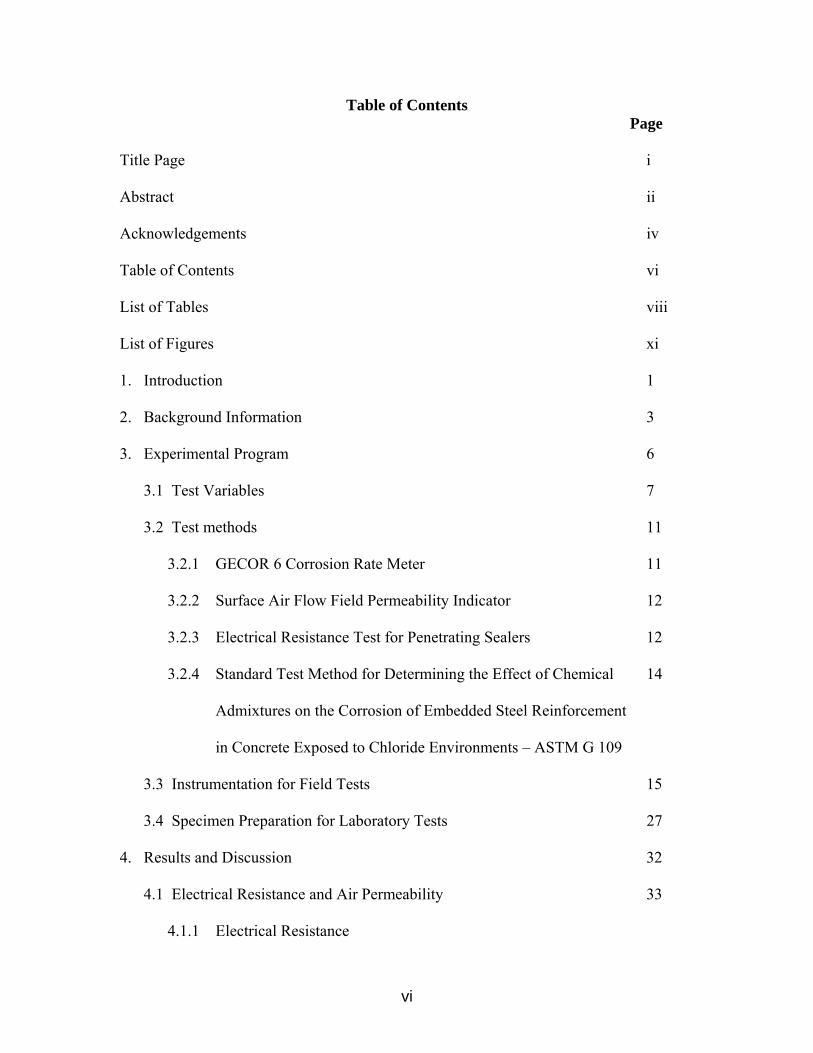
Table of Contents Page
Title Page i Abstract ii Acknowledgements iv Table of Contents vi List of Tables viii List of Figures xi 1. Introduction 1 2. Background Information 3 3. Experimental Program 6
3.1 Test Variables 7
3.2 Test methods 11
3.2.1 GECOR 6 Corrosion Rate Meter 11
3.2.2 Surface Air Flow Field Permeability Indicator 12
3.2.3 Electrical Resistance Test for Penetrating Sealers 12
3.2.4 Standard Test Method for Determining the Effect of Chemical 14
Admixtures on the Corrosion of Embedded Steel Reinforcement
in Concrete Exposed to Chloride Environments – ASTM G 109
3.3 Instrumentation for Field Tests 15
3.4 Specimen Preparation for Laboratory Tests 27
4. Results and Discussion 32
4.1 Electrical Resistance and Air Permeability 33
4.1.1 Electrical Resistance

vii
4.1.2 Air Permeability 34
4.2 Corrosion Measurements 40
4.3 Performance of Corrosion Inhibitors: Further Analysis 52
5. Conclusions and Recommendations 54
5.1 Conclusions 54
5.2 Recommendations 54
6. References 57
7. Appendix 59

viii
List of Tables Page
Table 3.1: Bridge Locations with corresponding Corrosion Inhibiting 7 Admixtures and Reinforcing Steel Type Table 3.2: Mix Design of North Main Street – Westbound 8 Table 3.3: Mix Design of North Main Street – Eastbound 8 Table 3.4: Mix Design of Wyckoff Road – Westbound 9 Table 3.5: Mix Design of Wyckoff Road – Eastbound 9 Table 3.6: Mix Design of Route 130 – Westbound 10 Table 3.7: Table 3.7: Minideck Sample Location. 31
Table 4.1: Fresh Concrete Properties 32 Table 4.2: Hardened Concrete properties 32 Table 4.3: R Square Values for Corrosion Rate and Corrosion Potential 52 Table 4.4: R Square Values for the Correlation between the Logarithm of time 53
and the Corrosion Rate and Corrosion Potential
Table A.1: Interpretation of Corrosion Rate Data (Scannell, 1997) 62
Table A.2: Interpretation of Half Cell (Corrosion) Potential Readings 62
(ASTM C 876)
Table B.1: Interpretation of Corrosion rate data (Scannell, 1997) 64
Table B.2: Interpretation of Half Cell (Corrosion) Potential Readings 64
(ASTM C 876)
Table B.3: Relative Concrete Permeability by Surface Air Flow 64
Table C.1: Relative Concrete Permeability by Surface Air Flow 70
Table D.1: Preliminary DC Testing of Gauge (Scannell, 1996) 73
Table F.1: North Main Street Westbound GECOR 6 Electrical Resistance (KΩ) 87
Table F.2: North Main Street Westbound Air Permeability 88 Vacuum (mm Hg), SCCM (ml/min)

ix
Table F.3: North Main Street Westbound Electrical Resistance Sealer Test (kΩ) 88
Table F.4: North Main Street Eastbound GECOR 6 Electrical Resistance (KΩ) 89
Table F.5: North Main Street Eastbound Air Permeability 90
Vacuum (mm Hg), SCCM (ml/min)
Table F.6: North Main Street Eastbound Electrical Resistance Sealer Test (KΩ) 90
Table F.7: Wyckoff Road Westbound GECOR 6 Electrical Resistance (KΩ) 91
Table F.8: Wyckoff Road Westbound Air Permeability Vacuum (mm Hg), 92
SCCM (ml/min)
Table F.9: Wyckoff Road Westbound Electrical Resistance Sealer Test (KΩ) 92
Table F.10: Wyckoff Road Eastbound GECOR 6 Electrical Resistance (KΩ) 93
Table F.11: Wyckoff Road Eastbound Air Permeability Vacuum (mm Hg), 94
SCCM (ml/min)
Table F.12: Wyckoff Road Eastbound Electrical Resistance Sealer Test (KΩ) 94
Table F.13: Route 130 Westbound GECOR Electrical Resistance (KΩ) 95
Table F.14: Route 130 Westbound Air Permeability Vacuum (mm Hg), 96
SCCM (ml/min)
Table F.15: Route 130 Westbound Electrical Resistance Sealer Test (KΩ) 96
Table G.1: Minideck A – ASTM G 109 Corrosion Rate (µA/cm2) 98
Table G.2: Minideck A – ASTM G 109 Corrosion Potential (mV) 99
Table G.3: North Main Street Westbound GECOR 6 Corrosion Rate (µA/cm2) 101
Table G.4: Main Street Westbound GECOR 6 Corrosion Potential (mV) 102
Table G.5: Minideck B – ASTM G 109 Corrosion Rate (µA/cm2) 104
Table G.6: Minideck B – ASTM G 109 Corrosion Potential (mV) 105
Table G.7: North Main Street Eastbound GECOR 6 Corrosion Rate (µA/cm2) 107
Table G.8: North Main Street Eastbound GECOR 6 Corrosion Potential (mV) 108
Table G.9: Minideck C –ASTM G 109 Corrosion Rate (µA/cm2) 110
Table G.10: Minideck C – ASTM G 109 Corrosion Potential (mV) 111
Table G.11: Wyckoff Road Westbound GECOR 6 Corrosion Rate (µA/cm2) 113
Table G.12: Wyckoff Road Westbound GECOR 6 Corrosion Potential (mV) 114
Table G.13: Minideck D – ASTM G 109 Corrosion Rate (µA/cm2) 116
Table G.14: Minideck D – ASTM G 109 Corrosion Potential (mV) 117
x
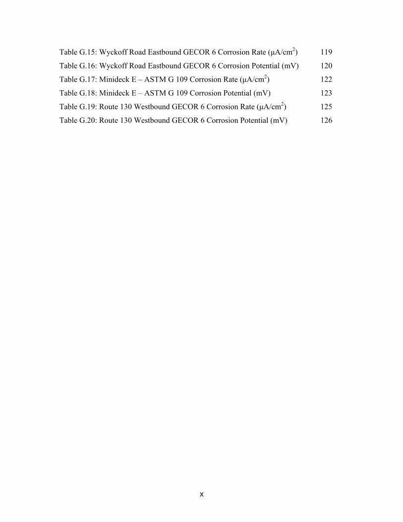
Table G.15: Wyckoff Road Eastbound GECOR 6 Corrosion Rate (µA/cm2) 119
Table G.16: Wyckoff Road Eastbound GECOR 6 Corrosion Potential (mV) 120
Table G.17: Minideck E – ASTM G 109 Corrosion Rate (µA/cm2) 122
Table G.18: Minideck E – ASTM G 109 Corrosion Potential (mV) 123
Table G.19: Route 130 Westbound GECOR 6 Corrosion Rate (µA/cm2) 125
Table G.20: Route 130 Westbound GECOR 6 Corrosion Potential (mV) 126
xi
List of Figures Page
Fig. 3.1: Strips of Silver Conductive Paint 12
Fig. 3.2: View of Concrete Minideck (ASTM G 109) 14
Fig. 3.3: Locations of GECOR 6 Corrosion Rate Meter Tests 16
Fig. 3.4: Locations of GECOR 6 Corrosion Rate Meter Tests 16
Fig. 3.5: Locations of GECOR 6 Corrosion Rate Meter Tests 17
Fig. 3.6: Locations of GECOR 6 Corrosion Rate Meter Tests 17
Fig. 3.7: Locations of GECOR 6 Corrosion Rate Meter Tests 18
Fig. 3.8: Locations of Uncoated Steel Reinforcement Bars on 18
Route 130 Westbound
Fig. 3.9: Insulated Copper Underground Feeder Cables 19
Fig. 3.10: Locations of Surface Air Flow Field Permeability Indicator Readings 21
Fig. 3.11: Locations of Surface Air Flow Field Permeability Indicator Readings 21
Fig. 3.12: Locations of Surface Air Flow Field Permeability Indicator Readings 22
Fig. 3.13: Locations of Surface Air Flow Field Permeability Indicator Readings 22
Fig. 3.14: Locations of Surface Air Flow Field Permeability Indicator Readings 23
Fig. 3.15: Locations of Electrical Resistance Tests 24
Fig. 3.16: Locations of Electrical Resistance Tests 24
Fig. 3.17: Locations of Electrical Resistance Tests 25
Fig. 3.18: Locations of Electrical Resistance Tests 25
Fig. 3.19: Locations of Electrical Resistance Tests 26
Fig. 3.20: Prepared Minideck Mold 27
Fig. 3.21: Minideck after Removal from Mold 28
Fig. 3.22: View of Plexiglas Dam 29
Fig.3.23: Ponded Minideck Samples 30
Fig. 4.1: North Main Street Westbound Average Electrical Resistance AC (KΩ) 35
Fig. 4.2: North Main Street Eastbound Average Electrical Resistance AC (KΩ) 35
Fig. 4.3: Wyckoff Road Westbound Average Electrical Resistance AC (KΩ) 36
Fig. 4.4: Wyckoff Road Eastbound Average Electrical Resistance AC (KΩ) 36
Fig. 4.5: Route 130 Westbound Average Electrical Resistance AC (KΩ) 37
xii
Fig. 4.6: North Main Street Westbound Average Air Flow Rate (ml/min) 37
Fig. 4.7: North Main Street Eastbound Average Air Flow Rate (ml/min) 38
Fig. 4.8: Wyckoff Road Westbound Average Air Flow Rate (ml/min) 38
Fig. 4.9: Wyckoff Road Westbound Average Air Flow Rate (ml/min) 39
Fig. 4.10: Route 130 Westbound Average Air Flow Rate (ml/min) 39
Fig 4.11: Minideck A – Average Corrosion Rate Macrocell Current (µA) 42
Fig 4.12: Minideck B – Average Corrosion Rate Macrocell Current (µA) 43
Fig. 4.13: Minideck C – Average Corrosion Rate Macrocell Current (µA) 44
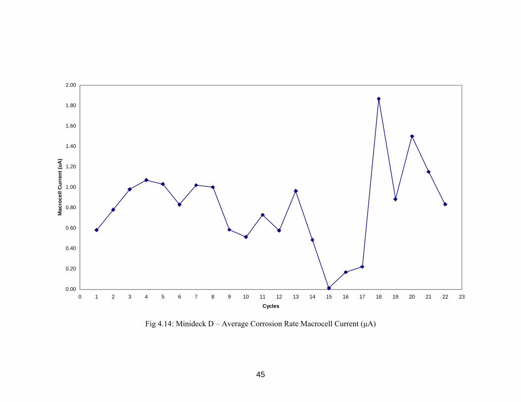
Fig 4.14: Minideck D – Average Corrosion Rate Macrocell Current (µA) 45
Fig. 4.15: Minideck E – Average Corrosion Rate Macrocell Current (µA) 46
Fig 4.16: North Main Street Westbound GECOR 6 Average 47
Corrosion Rate Macrocell Current (µA)
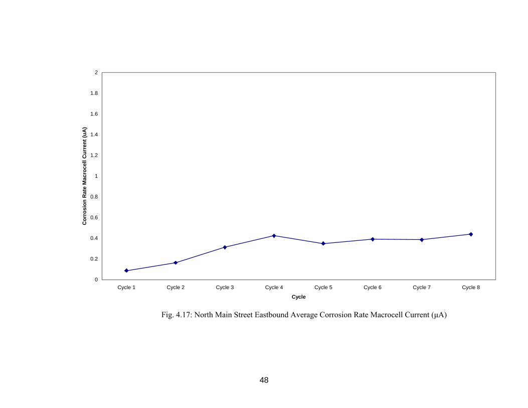
Fig. 4.17: North Main Street Eastbound Average 48
Corrosion Rate Macrocell Current (µA)
Fig. 4.18: Wyckoff Road Westbound GECOR 6 Average Corrosion 50
Rate Macrocell Current (µA)
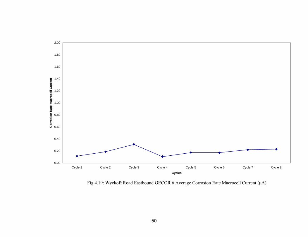
Fig 4.19: Wyckoff Road Eastbound GECOR 6 Average Corrosion 51
Rate Macrocell Current (µA)
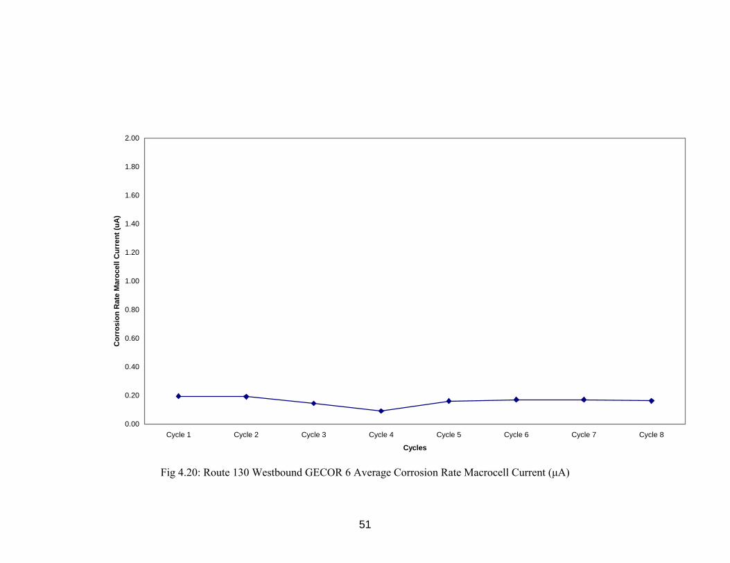
Fig 4.20: Route 130 Westbound GECOR 6 Average Corrosion 52
Rate Macrocell Current (µA)
Fig.C.1: Surface Air Flow Field Permeability Indicator (Front View) 63
Fig.C.2: Surface Air Flow Field Permeability Indicator (Front View) 63
Fig.C.3: Surface Air Flow Field Permeability Indicator 65
Fig.C.4: Drawing of Concrete Surface Air Flow Permeability Indicator 66
Fig.C.5: Schematic of Concrete Surface Air Flow Permeability Indicator 67
Fig.D.1: Equipment Required for Electrical Resistance Test 67
for Penetrating Sealers
Fig.E.1: Connection to North Main Street Westbound 68
Fig.E.2: Connection to North Main Street Eastbound 71
Fig.E.3: Connection to Wyckoff Road Westbound 75

xiii
Fig.E.4: Connection to Wyckoff Road Eastbound Fig.E.5: Connection 76
to Route 130 Westbound
Fig.E.6: Conduits and Enclosure – North Main Street Westbound 77
Fig.E.7: Conduits and Enclosure – North Main Street Eastbound 78
Fig.E.8: Conduits and Enclosure – Wyckoff Road Westbound 79
Fig.E.9: Conduits and Enclosure – Wyckoff Road Eastbound 80
Fig.E.10: Conduits and Enclosure – Route 130 Westbound 80
Fig.E.11: Vibrating of Fresh Concrete at North Main Street Eastbound 81
Fig.E.12: Placement of Fresh Concrete at North Main Street Westbound 81
Fig.E.13: View of Connections at North Main Street Westbound during 82
Concrete Placement
Fig.E.14: Bridge Deck over North Main Street Westbound near Completion 83
Fig.E.15: Bridge Deck over North Main Street Eastbound near Completion 83
Fig.E.16: Bridge Deck over Wyckoff Road Westbound near Completion 84
Fig.E.17: Bridge Deck over Wyckoff Road Eastbound near Completion 84
Fig.E.18: Bridge Deck over Rout 130 Westbound near Completion 85
Fig G.1: Minideck A – Average Corrosion Potential (mV) 100
Fig G.2: North Main Street Westbound GECOR 6 103
Average Corrosion Potential (mV)
Fig. G.3: Minideck B – Average Corrosion Potential (mV) 106
Fig. G.4: North Main Street Eastbound GEOCOR 6 109
Average Corrosion Potential
Fig G.5: Minideck C – Average Corrosion Potential (mV) 112
Fig G.6: Wyckoff Road Westbound GECOR 6 115
Average Corrosion Potential (mV)
Fig. G.7: Minideck D – Average Corrosion Potential (mV) 118
Fig G.8: Wyckoff Road Eastbound GECOR 6 121
Average Corrosion Potential (mV)
Fig. G.9: Minideck E – Average Corrosion Potential (mV) 124
Fig G.10: Route 130 Westbound GECOR 6 127
Average Corrosion Potential (mV)

1
1. Introduction
Corrosion of reinforcement is a global problem that has been studied extensively.
Though the high alkali nature of concrete normally protects reinforcing steel with the
formation of a tightly adhering film which passivates the steel and protects it from
corrosion, the harsh environment in the Northeastern United States and similar locations
around the world accelerate the corrosion process. The major techniques used for
reducing corrosion and preventing it to some extent are: (i) Use of concrete with least
permeability, (ii) Use corrosion inhibitors, (iii) Use of epoxy coated bars, (iv) Surface
protection of concrete, and (v) Cathodic protection of reinforcement. Use the nonmetallic
reinforcement is one more technique to reduce corrosion, which is still in development
stage.
The use of inhibitors to control the corrosion of concrete is a well-established
technology. Inhibitors are in effect any materials that are able to reduce the corrosion
rates present at relatively small concentrations at or near the steel surface. When
correctly specified and applied by experienced professionals, inhibitors can be effective
for use in both the repair of deteriorating concrete structures and enhancing the durability
of new structures.
The use of good quality concrete and corrosion inhibitors seems to be an
economical, effective, and logical solution, especially for new structures. The objective
of this study is to determine the effectiveness of four different corrosion inhibitors to
reduce corrosion of the structural steel reinforcement in a structure. The data is
compared with the data from structural steel reinforcement not protected by a corrosion
inhibitor.
1.1 Objective
The primary objective of the research program is to evaluate the effectiveness of
the latest corrosion inhibiting admixtures for steel reinforced concrete using laboratory
and field study. It was envisioned that the laboratory accelerated test will provide
effectiveness of the commercially available corrosion inhibitors, and these results can be

2
used to predict the behavior of bridge decks. The bridge decks were instrumented to
measure corrosion levels and the results from these decks were to be correlated with
laboratory results.
3
2. Background Information
Steel reinforced concrete is one of the most durable and cost effective
construction materials. The alkaline environment of the concrete passivates the steel
resulting in reduction of corrosion activity in steel. However, concrete is often utilized in
extreme environments in which it is subjected to exposure to chloride ions, which disrupt
the passivity (Berke, 1995). Though corrosion inhibitors are one of the most practical
and effective means to arrest the corrosion process in old and new reinforced concrete,
the use of good quality concrete is also very significant in inhibiting corrosion. Concrete
with low water to cement ratios can lower the amount of chloride ingress. Pozzolans
such as silica-fume increases concrete resistively and permeably to chloride (Berke,
1995).
The principle of most inhibitors is to develop a thin chemical layer usually one or
two molecules thick on the steel surface that inhibits the corrosion attack. Inhibitors can
prevent the cathodic reaction, the anodic reaction, or both. They are consumed and will
only work up to a given level of attack. The chloride content of the concrete determines
the level of attack (Broomfield, 1997).
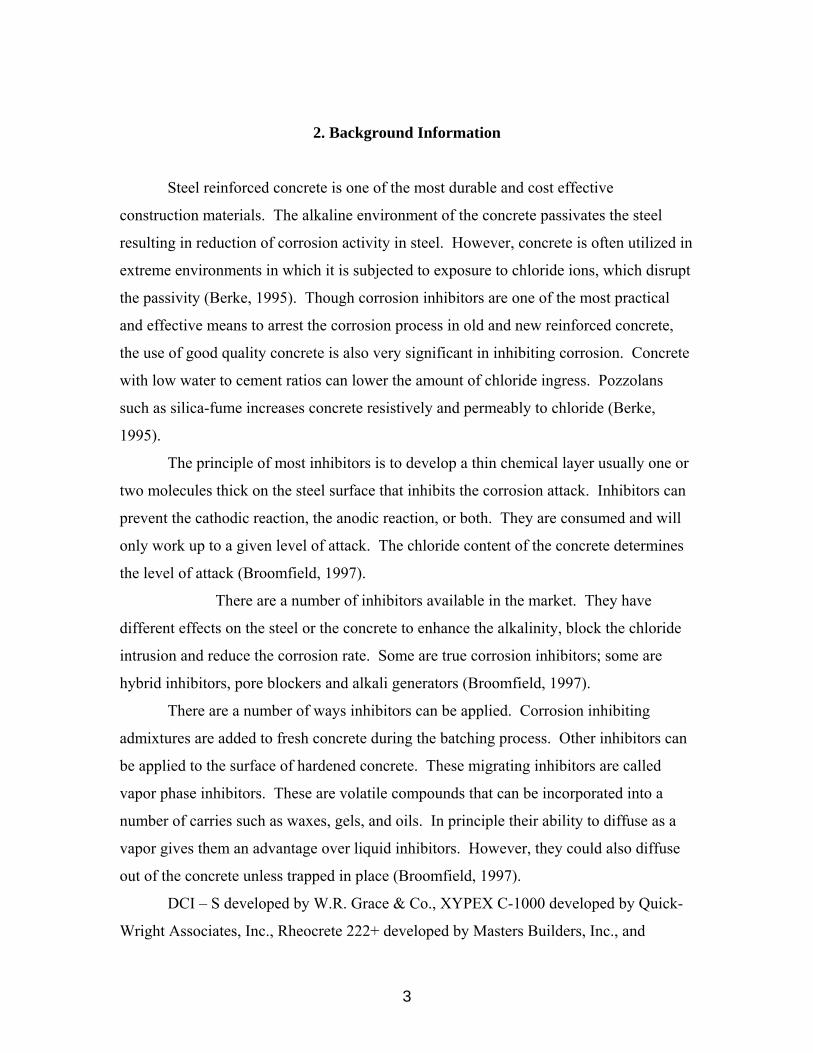
There are a number of inhibitors available in the market. They have
different effects on the steel or the concrete to enhance the alkalinity, block the chloride
intrusion and reduce the corrosion rate. Some are true corrosion inhibitors; some are
hybrid inhibitors, pore blockers and alkali generators (Broomfield, 1997).
There are a number of ways inhibitors can be applied. Corrosion inhibiting
admixtures are added to fresh concrete during the batching process. Other inhibitors can
be applied to the surface of hardened concrete. These migrating inhibitors are called
vapor phase inhibitors. These are volatile compounds that can be incorporated into a
number of carries such as waxes, gels, and oils. In principle their ability to diffuse as a
vapor gives them an advantage over liquid inhibitors. However, they could also diffuse
out of the concrete unless trapped in place (Broomfield, 1997).
DCI – S developed by W.R. Grace & Co., XYPEX C-1000 developed by Quick-
Wright Associates, Inc., Rheocrete 222+ developed by Masters Builders, Inc., and
4
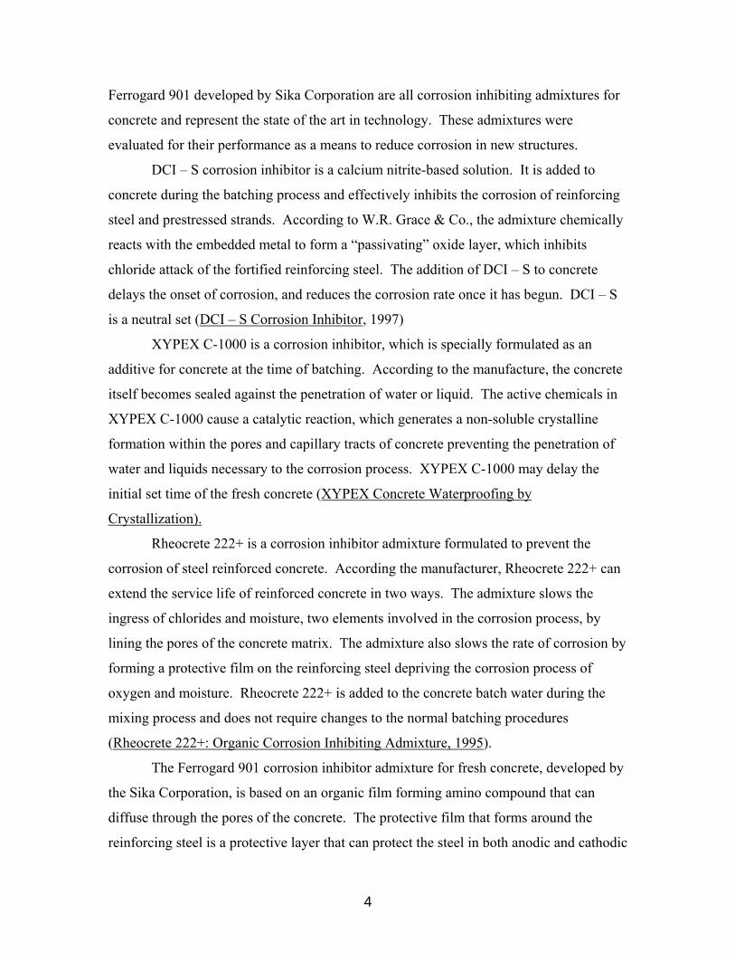
Ferrogard 901 developed by Sika Corporation are all corrosion inhibiting admixtures for
concrete and represent the state of the art in technology. These admixtures were
evaluated for their performance as a means to reduce corrosion in new structures.
DCI – S corrosion inhibitor is a calcium nitrite-based solution. It is added to
concrete during the batching process and effectively inhibits the corrosion of reinforcing
steel and prestressed strands. According to W.R. Grace & Co., the admixture chemically
reacts with the embedded metal to form a “passivating” oxide layer, which inhibits
chloride attack of the fortified reinforcing steel. The addition of DCI – S to concrete
delays the onset of corrosion, and reduces the corrosion rate once it has begun. DCI – S
is a neutral set (DCI – S Corrosion Inhibitor, 1997)
XYPEX C-1000 is a corrosion inhibitor, which is specially formulated as an
additive for concrete at the time of batching. According to the manufacture, the concrete
itself becomes sealed against the penetration of water or liquid. The active chemicals in
XYPEX C-1000 cause a catalytic reaction, which generates a non-soluble crystalline
formation within the pores and capillary tracts of concrete preventing the penetration of
water and liquids necessary to the corrosion process. XYPEX C-1000 may delay the
initial set time of the fresh concrete (XYPEX Concrete Waterproofing by
Crystallization).
Rheocrete 222+ is a corrosion inhibitor admixture formulated to prevent the
corrosion of steel reinforced concrete. According the manufacturer, Rheocrete 222+ can
extend the service life of reinforced concrete in two ways. The admixture slows the
ingress of chlorides and moisture, two elements involved in the corrosion process, by
lining the pores of the concrete matrix. The admixture also slows the rate of corrosion by
forming a protective film on the reinforcing steel depriving the corrosion process of
oxygen and moisture. Rheocrete 222+ is added to the concrete batch water during the
mixing process and does not require changes to the normal batching procedures
(Rheocrete 222+: Organic Corrosion Inhibiting Admixture, 1995).
The Ferrogard 901 corrosion inhibitor admixture for fresh concrete, developed by
the Sika Corporation, is based on an organic film forming amino compound that can
diffuse through the pores of the concrete. The protective film that forms around the
reinforcing steel is a protective layer that can protect the steel in both anodic and cathodic

5
areas. According to the manufacturer, this Ferrogard 901 suppresses the electrochemical
corrosion reaction and shows no detrimental effects to the concrete (MacDonald, 1996).
DCI-S, Rheocrete 222+, and Ferrogard 911 are primarily made of organic
products. The organic substances form a coating around the steel and provide protection.
XYPEX C-2000 consists of Portland cement, very fine treated silica and various active
proprietary chemicals. These active chemicals react with the moisture in concrete
forming non soluble crystalline formation in the concrete pores.

6
3. Experimental Program
The primary objective of the research program is to evaluate the effectiveness of
the latest corrosion inhibiting admixtures for steel reinforced concrete using laboratory
and field study. It was envisioned that the laboratory accelerated test will provide
effectiveness of the commercially available corrosion inhibitors, and these results can be
used to predict the behavior of bridge decks. The bridge decks were instrumented to
measure corrosion levels and the results from these decks were to be correlated with
laboratory results.
The test variables are the four corrosion-inhibiting admixtures mentioned in
chapter 2. These were incorporated in bridge decks during the construction of the bridge
decks on the route 133 Hightstown Bypass. One deck was constructed with no corrosion-
inhibiting admixture, which served as control.
The field evaluation consists of three tests: GECOR 6 Corrosion Rate Meter,
Surface Air Flow Permeability Indicator, and Electrical Resistance Test for Penetrating
Sealers. The results of these tests can be used to determine the physical characters as
well as the corrosion protection provided by a particular admixture. The bridges were
instrumented for corrosion testing and are periodically monitored for corrosion activity.
The laboratory samples were tested using ASTM G 109. This accelerated process will
give an early indication of the effectiveness of the admixtures. All the concrete samples
were taken from the field as the concrete for the individual bridge decks was placed.
Fresh concrete was tested for workability and air content. Compressive strength
was obtained at 28 days. The parameters studied were corrosion rate, corrosion potential,
air permeability, and electrical resistance.
7
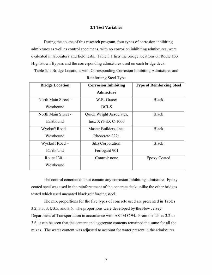
3.1 Test Variables
During the course of this research program, four types of corrosion inhibiting
admixtures as well as control specimens, with no corrosion inhibiting admixtures, were
evaluated in laboratory and field tests. Table 3.1 lists the bridge locations on Route 133
Hightstown Bypass and the corresponding admixtures used on each bridge deck.
Table 3.1: Bridge Locations with Corresponding Corrosion Inhibiting Admixtures and
Reinforcing Steel Type
Bridge Location Corrosion Inhibiting
Admixture
Type of Reinforcing Steel
North Main Street -
Westbound
W.R. Grace:
DCI-S
Black
North Main Street -
Eastbound
Quick Wright Associates,
Inc.: XYPEX C-1000
Black
Wyckoff Road –
Westbound
Master Builders, Inc.:
Rheocrete 222+
Black
Wyckoff Road –
Eastbound
Sika Corporation:
Ferrogard 901
Black
Route 130 –
Westbound
Control: none Epoxy Coated
The control concrete did not contain any corrosion-inhibiting admixture. Epoxy
coated steel was used in the reinforcement of the concrete deck unlike the other bridges
tested which used uncoated black reinforcing steel.
The mix proportions for the five types of concrete used are presented in Tables
3.2, 3.3, 3.4, 3.5, and 3.6. The proportions were developed by the New Jersey
Department of Transportation in accordance with ASTM C 94. From the tables 3.2 to
3.6, it can be seen that the cement and aggregate contents remained the same for all the
mixes. The water content was adjusted to account for water present in the admixtures.

8
Table 3.2: Mix Design of North Main Street – Westbound (Corrosion Inhibitor: DCI-S)
Bridge Deck over North Main Street – Westbound
Date of Deck Pour: May 6, 1998
Cements (lbs) 700
Sand (lbs) 1346
¾ in. Aggregate (lbs) 1750
Water (gal) 29.3
W/C Ratio 0.38
Sika Corporation AER Air-Entraining Admixture ASTM C-150 (oz) 6.3
Sika Corporation Plastocrete 161 Water reducing Admixture Type
“A” ASTM C 494 (oz)
21
W.R. Grace: DCI-S (gal) 3
Slump (inches) 3+1
Air (%) 6+1.5
Table 3.3: Mix Design of North Main Street – Eastbound (Corrosion Inhibitor: XYPEX
C-1000)
Bridge Deck over North Main Street – Eastbound
Date of Deck Pour: May 14, 1998
Cements (lbs) 700
Sand (lbs) 1346
¾ in. Aggregate (lbs) 1750
Water (gal) 31.8
W/C Ratio 0.38
Sika Corporation AER Air-Entraining Admixture ASTM C-150 (oz) 4.2
Sika Corporation Plastocrete 161 Water reducing Admixture Type
“A” ASTM C 494 (oz)
21
Quick Wright Associates, Inc.: XYPEX C-1000 (lbs) 12
Slump (inches) 3+1
Air (%) 6+1.5
9
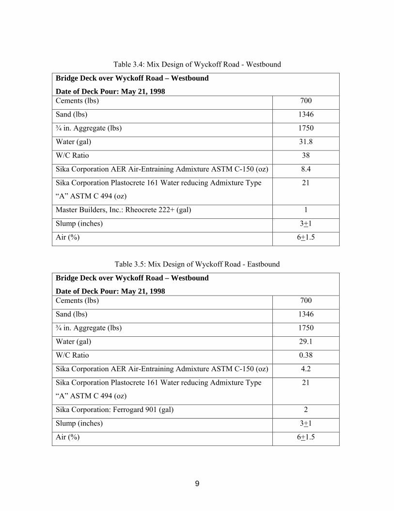
Table 3.4: Mix Design of Wyckoff Road - Westbound
Bridge Deck over Wyckoff Road – Westbound
Date of Deck Pour: May 21, 1998 Cements (lbs) 700
Sand (lbs) 1346
¾ in. Aggregate (lbs) 1750
Water (gal) 31.8
W/C Ratio 38
Sika Corporation AER Air-Entraining Admixture ASTM C-150 (oz) 8.4
Sika Corporation Plastocrete 161 Water reducing Admixture Type
“A” ASTM C 494 (oz)
21
Master Builders, Inc.: Rheocrete 222+ (gal) 1
Slump (inches) 3+1
Air (%) 6+1.5
Table 3.5: Mix Design of Wyckoff Road - Eastbound
Bridge Deck over Wyckoff Road – Westbound
Date of Deck Pour: May 21, 1998 Cements (lbs) 700
Sand (lbs) 1346
¾ in. Aggregate (lbs) 1750
Water (gal) 29.1
W/C Ratio 0.38
Sika Corporation AER Air-Entraining Admixture ASTM C-150 (oz) 4.2
Sika Corporation Plastocrete 161 Water reducing Admixture Type
“A” ASTM C 494 (oz)
21
Sika Corporation: Ferrogard 901 (gal) 2
Slump (inches) 3+1
Air (%) 6+1.5
10
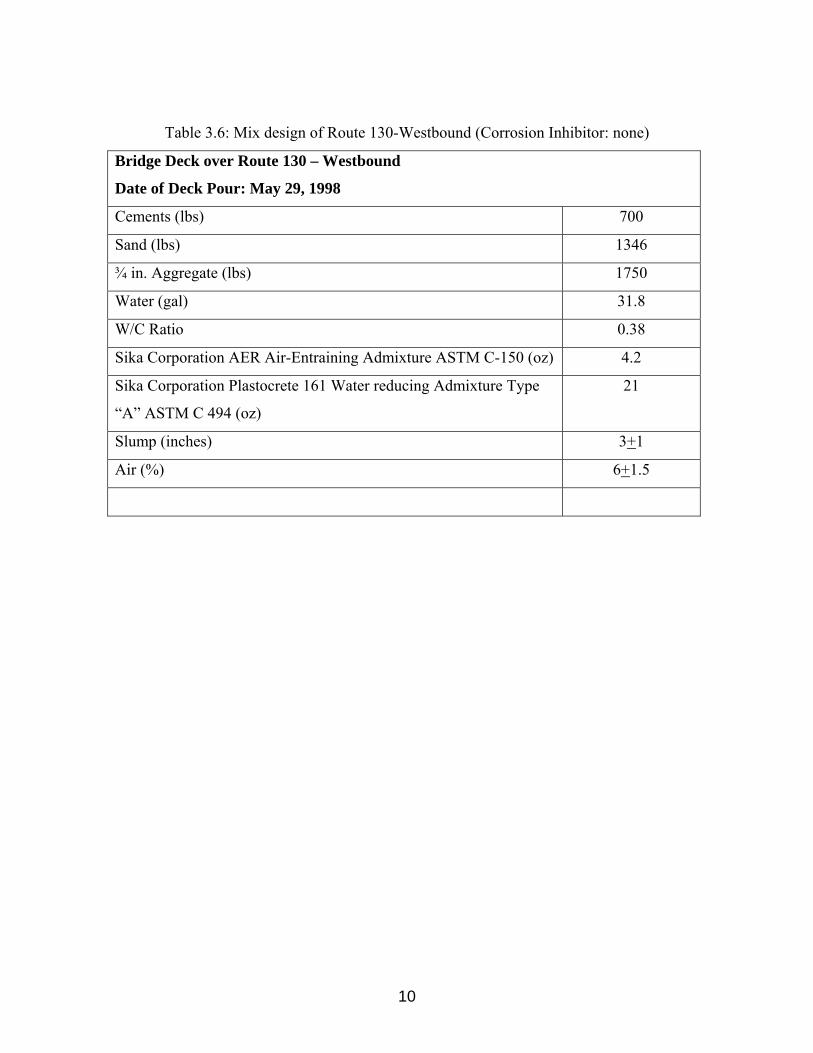
Table 3.6: Mix design of Route 130-Westbound (Corrosion Inhibitor: none)
Bridge Deck over Route 130 – Westbound
Date of Deck Pour: May 29, 1998
Cements (lbs) 700
Sand (lbs) 1346
¾ in. Aggregate (lbs) 1750
Water (gal) 31.8
W/C Ratio 0.38
Sika Corporation AER Air-Entraining Admixture ASTM C-150 (oz) 4.2
Sika Corporation Plastocrete 161 Water reducing Admixture Type
“A” ASTM C 494 (oz)
21
Slump (inches) 3+1
Air (%) 6+1.5

11
3.2 Test Methods
The test procedures used are described in the following sections. The first three
tests were conducted in the field where as the fourth one was conducted in the laboratory.
The laboratory test provides the information on corrosion potential which can be
used to estimate the effectiveness of corrosion inhibitors. The air permeability and the
electrical resistance test conducted in the field were used to determine possible variations
in permeability and uniformity of concrete in the five bridge decks chosen for the study.
Corrosion rate measured in the field can be used to correlate the laboratory test results
that were obtained using accelerated corrosion.
3.2.1 GECOR Corrosion Rate Meter
The GECOR 6 Corrosion rate Meter provides valuable insight into the kinematics
of the corrosion process. Based on a steady state linear polarization technique it provides
information on the rate of the deterioration process. The meter monitors the
electrochemical process of corrosion to determine the rate of deterioration. This
nondestructive technique works by applying a small current to the reinforcing bar and
measuring the change in the half-cell potential. The corrosion rate, corrosion potential
and electrical resistance are provided by the corrosion rate meter.
Description of the equipment and test procedure is presented in Appendix A.
3.2.2 Surface Air Flow Field Permeability Indicator
The Concrete Surface Air Flow (SAF) Permeability Indicator is a nondestructive
technique designed to give an indication of the relative permeability of flat concrete
surfaces. The SAF can be utilized to determine the permeability of concrete slabs,
support members, bridge decks, and pavement (Manual for the Operation of a Surface
Air Flow Field Permeability Indicator, 1994). The concrete permeability is based on
airflow out of the concrete surface under an applied vacuum. The depth of measurement
was determined to be approximately 0.5in. below the concrete surface. A study between

12
the relationships between SAF readings and air and water permeability determined that
there is a good correlation in the results. As stated in the Participant’s Workbook:
FHWA-SHRP Showcase, (Scannell, 1996) the SAF should not be used as a substitute for
actual laboratory permeability testing. Cores tested under more standardized techniques
will provide a more accurate value for permeability due the fact that the effects of surface
texture and micro cracks have not been fully studied for the SAF.
The SAF can determine permeability of both horizontal surfaces, by use of an
integral suction foot, and vertical surfaces, by use of external remote head. The remote
head was not used for this project. A description of the equipment and the test procedure
are presented in Appendix C.
3.2.3 Electrical Resistance Test for Penetrating Sealers
Although the main use of this testing method is to determine the effectiveness of
concrete penetrating sealers, it can also indicate the resistance of unsealed concrete
surfaces. The resistance measurement is tested on two strips of conductive paint sprayed
onto the concrete surface to be tested by using a, Nilsson 400, soil resistance meter. The
spray pattern can be seen in Fig. 3.1.
Fig. 3.1: Strips of Silver Conductive Paint
The materials needed for this test and test procedure are presented in Appendix D
13
The higher the resistance the less potential for corrosion in the embedded steel
due to the higher density of the concrete and improved insulation against the
electrochemical process of corrosion. The collected data and a discussion on the
resistance indicated are presented and discussed in the Test Results and Discussions
chapter.
14
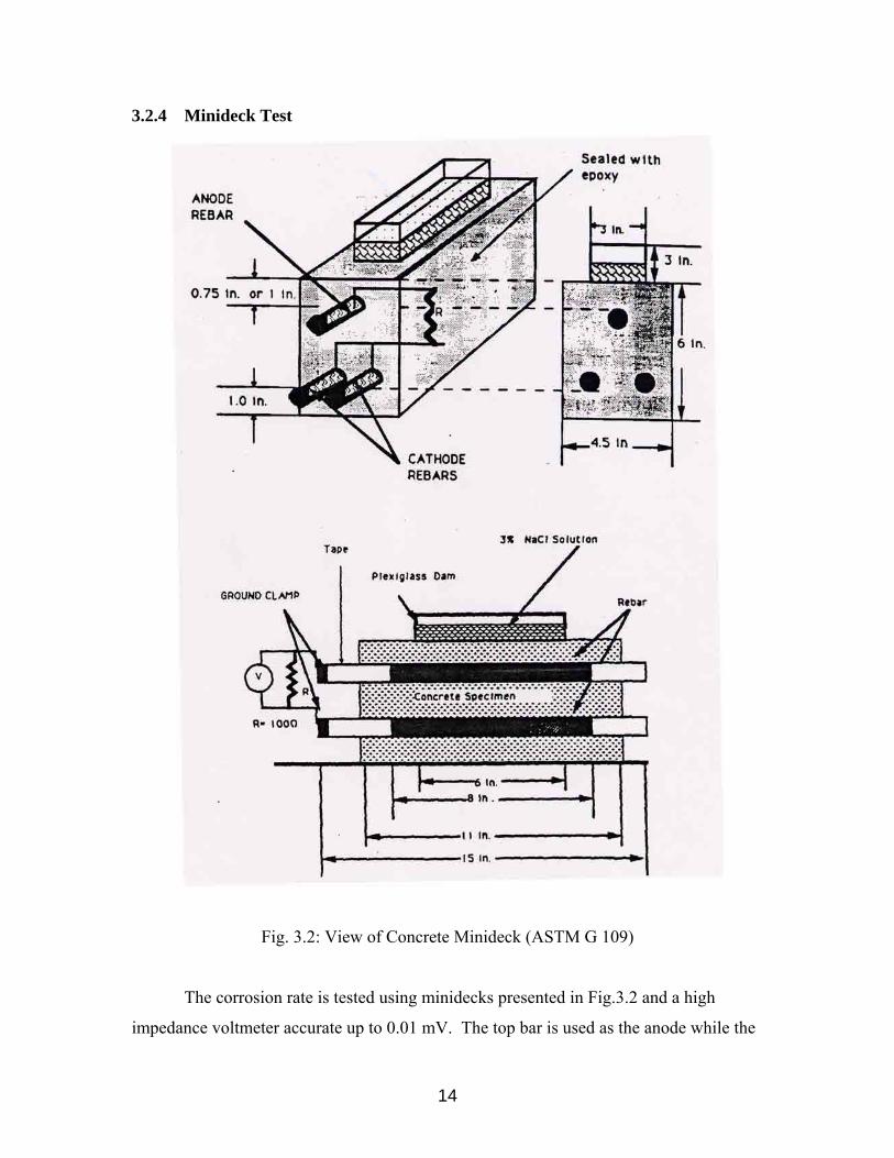
3.2.4 Minideck Test
Fig. 3.2: View of Concrete Minideck (ASTM G 109)
The corrosion rate is tested using minidecks presented in Fig.3.2 and a high
impedance voltmeter accurate up to 0.01 mV. The top bar is used as the anode while the
15
bottom bars are used as the cathode. Voltage is measured across a 100Ω resistor. The
current flowing, Ij, from the electrochemical process is calculated from the measured
voltage across the 100Ω resistor, Vj as:
Ij = Vj/100
The corrosion potential of the bars is measured against a reference electrode half-cell.
The electrode is placed in the dam containing the NaCl solution. The voltmeter is
connected between the electrodes and bars.
The current is monitored as a function of time until the average current of the
control specimens is 10 µA or Greater, and at least half the samples show currents equal
to or greater than 10 µA. The test is continued for a further three complete cycles to
ensure the presence of sufficient corrosion for a visual evaluation. At the conclusion of
the test, the minidecks are broken and the bars removed to assess the extent of corrosion
and to record the percentage of corroded area.
The results are interpreted with Table B.1 and Table B.2 in the Appendix. The
results of this test are presented in the results and Discussion Chapter.
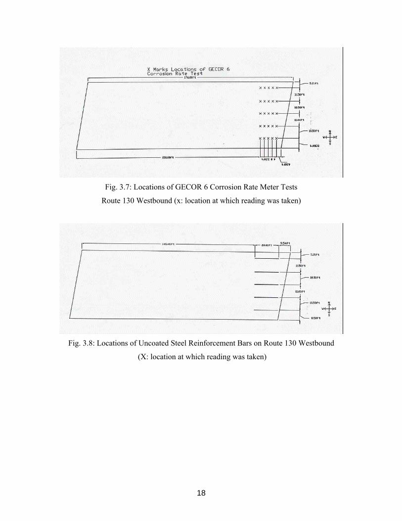
3.3 Instrumentation for Field Tests
Electrical connections were made to the top-reinforcing mat of each bridge deck
before the placement of the concrete. Five connections were made to Route 130
Westbound and four each on the remaining four bridges. A total of 105 readings were
taken per cycle using the GECOR 6 Corrosion Rate Meter. Twenty-five readings were
taken at the bridge deck over RT130 West Bound. Twenty readings each were taken at
the other four bridge decks tested. The locations of the tests are presented on Fig.3.3, 3.4,
3.5, 3.6, and 3.7. Due to the use of epoxy coated reinforcing bars on the bridge deck over
RT130 West Bound, it was necessary to place uncoated reinforcing bars into the top mat.
The locations of these bars are presented in Fig. 3.8. Short lengths of uncoated
reinforcing bars were welded to the existing reinforcement. The ends were tapped to
accept stainless steel nuts and bolts to attach underground copper feeder cables seen in
Fig. 3.9 that were used to connect the meter to the reinforcement in the bridge deck. To
ensure accurate readings, the connecting lengths of reinforcing bars were wire brushed to
16
remove the existing corrosion. They were then coated with epoxy and spray painted to
seal out moisture.
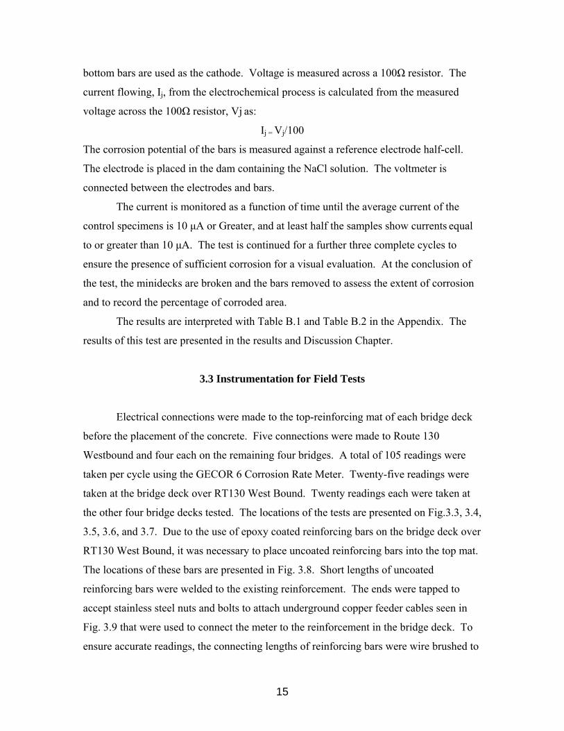
Fig. 3.3: Locations of GECOR 6 Corrosion Rate Meter Tests
North Main Street Westbound (x: location at which reading was taken)
Fig. 3.4: Locations of GECOR 6 Corrosion Rate Meter Tests
North Main Street Eastbound (x: location at which reading was taken)
17
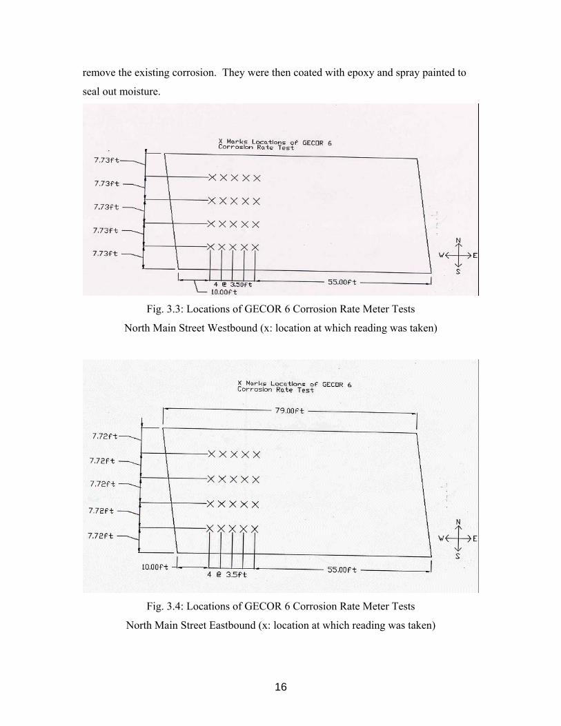
Fig. 3.5: Locations of GECOR 6 Corrosion Rate Meter Tests
Wyckoff Road Westbound (x: location at which reading was taken)
Fig. 3.6: Locations of GECOR 6 Corrosion Rate Meter Tests
Wyckoff Road Eastbound (x: location at which reading was taken)
18
Fig. 3.7: Locations of GECOR 6 Corrosion Rate Meter Tests
Route 130 Westbound (x: location at which reading was taken)
Fig. 3.8: Locations of Uncoated Steel Reinforcement Bars on Route 130 Westbound
(X: location at which reading was taken)

19
Fig. 3.9: Insulated Copper Underground Feeder Cables
20
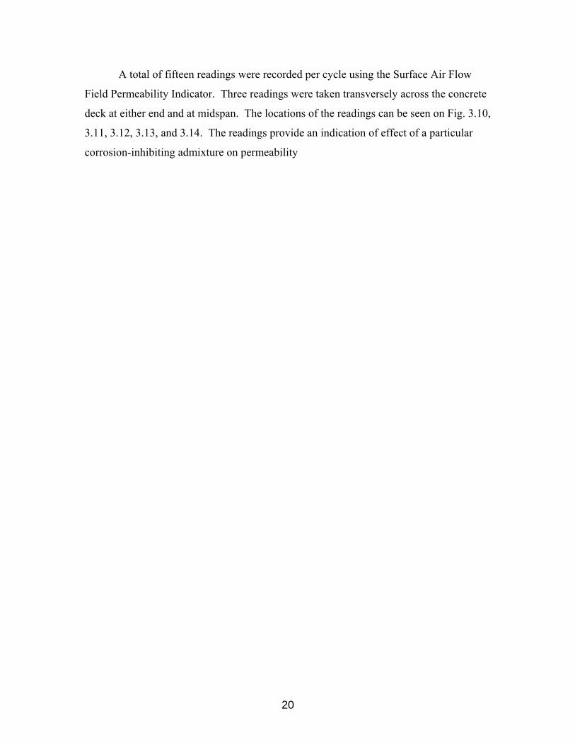
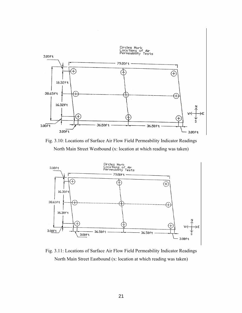
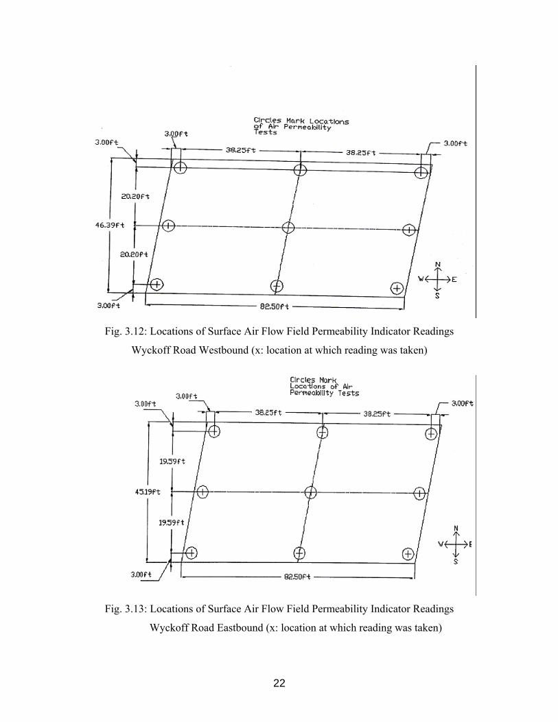
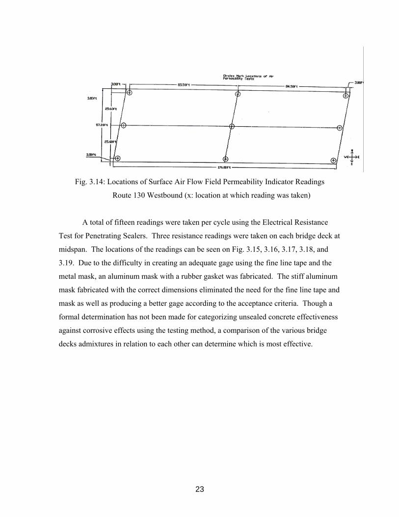
A total of fifteen readings were recorded per cycle using the Surface Air Flow
Field Permeability Indicator. Three readings were taken transversely across the concrete
deck at either end and at midspan. The locations of the readings can be seen on Fig. 3.10,
3.11, 3.12, 3.13, and 3.14. The readings provide an indication of effect of a particular
corrosion-inhibiting admixture on permeability
21
Fig. 3.10: Locations of Surface Air Flow Field Permeability Indicator Readings
North Main Street Westbound (x: location at which reading was taken)
Fig. 3.11: Locations of Surface Air Flow Field Permeability Indicator Readings
North Main Street Eastbound (x: location at which reading was taken)
22
Fig. 3.12: Locations of Surface Air Flow Field Permeability Indicator Readings
Wyckoff Road Westbound (x: location at which reading was taken)
Fig. 3.13: Locations of Surface Air Flow Field Permeability Indicator Readings
Wyckoff Road Eastbound (x: location at which reading was taken)
23
Fig. 3.14: Locations of Surface Air Flow Field Permeability Indicator Readings
Route 130 Westbound (x: location at which reading was taken)
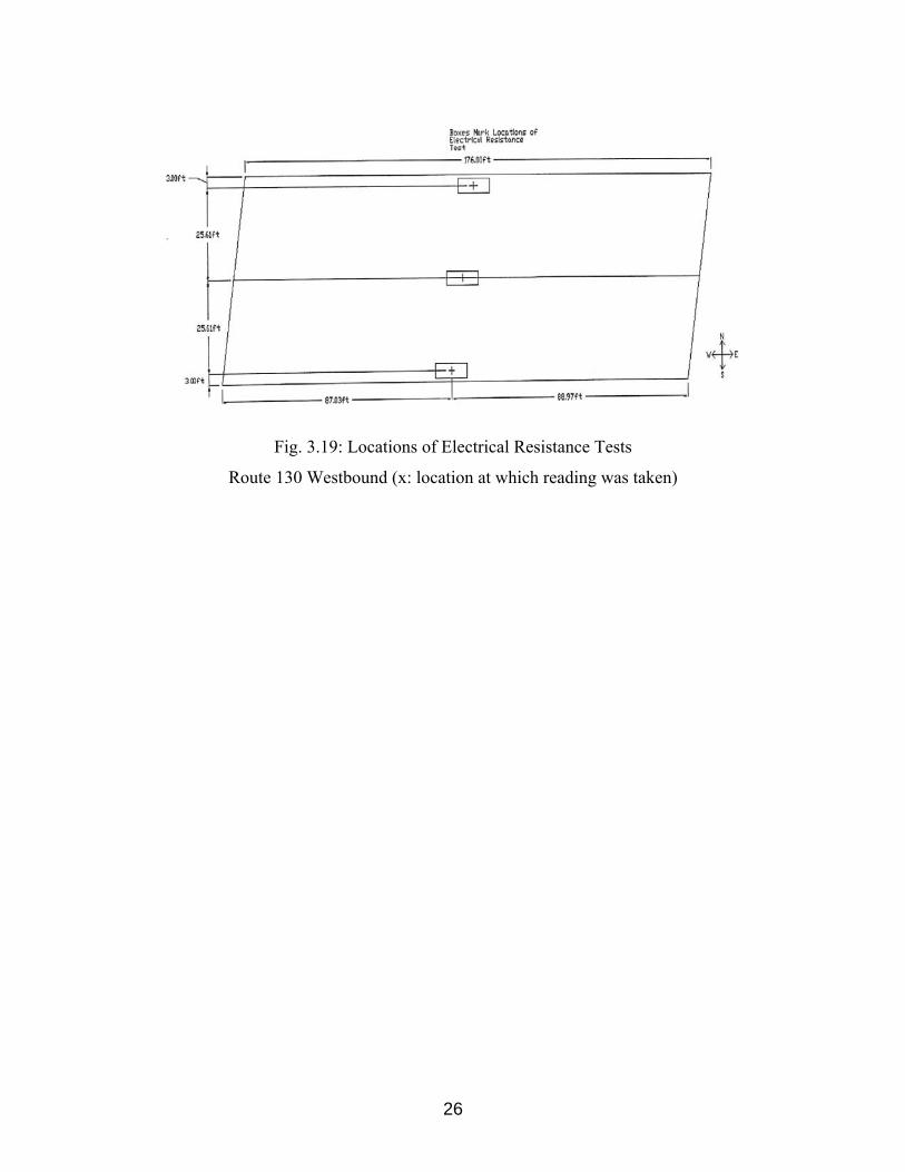
A total of fifteen readings were taken per cycle using the Electrical Resistance
Test for Penetrating Sealers. Three resistance readings were taken on each bridge deck at
midspan. The locations of the readings can be seen on Fig. 3.15, 3.16, 3.17, 3.18, and
3.19. Due to the difficulty in creating an adequate gage using the fine line tape and the
metal mask, an aluminum mask with a rubber gasket was fabricated. The stiff aluminum
mask fabricated with the correct dimensions eliminated the need for the fine line tape and
mask as well as producing a better gage according to the acceptance criteria. Though a
formal determination has not been made for categorizing unsealed concrete effectiveness
against corrosive effects using the testing method, a comparison of the various bridge
decks admixtures in relation to each other can determine which is most effective.

24
Fig. 3.15: Locations of Electrical Resistance Tests
North Main Street Westbound (x: location at which reading was taken)
Fig. 3.16: Locations of Electrical Resistance Tests
North Main Street Eastbound (x: location at which reading was taken)

25
Fig. 3.17: Locations of Electrical Resistance Tests
Wyckoff Road Westbound (x: location at which reading was taken)
Fig. 3.18: Locations of Electrical Resistance Tests
Wyckoff Road Eastbound (x: location at which reading was taken)
26
Fig. 3.19: Locations of Electrical Resistance Tests
Route 130 Westbound (x: location at which reading was taken)
27
3.4 Specimen Preparation for Laboratory Tests
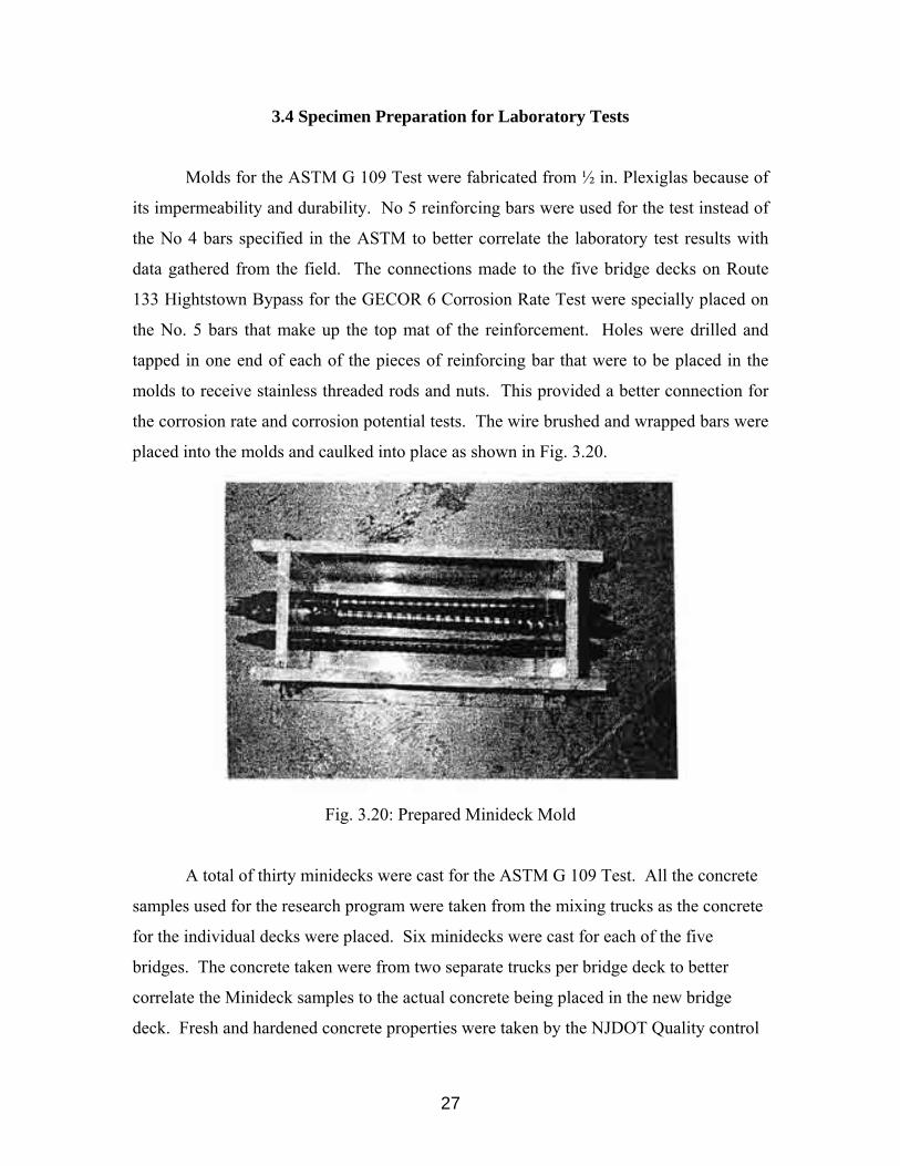
Molds for the ASTM G 109 Test were fabricated from ½ in. Plexiglas because of
its impermeability and durability. No 5 reinforcing bars were used for the test instead of
the No 4 bars specified in the ASTM to better correlate the laboratory test results with
data gathered from the field. The connections made to the five bridge decks on Route
133 Hightstown Bypass for the GECOR 6 Corrosion Rate Test were specially placed on
the No. 5 bars that make up the top mat of the reinforcement. Holes were drilled and
tapped in one end of each of the pieces of reinforcing bar that were to be placed in the
molds to receive stainless threaded rods and nuts. This provided a better connection for
the corrosion rate and corrosion potential tests. The wire brushed and wrapped bars were
placed into the molds and caulked into place as shown in Fig. 3.20.
Fig. 3.20: Prepared Minideck Mold
A total of thirty minidecks were cast for the ASTM G 109 Test. All the concrete
samples used for the research program were taken from the mixing trucks as the concrete
for the individual decks were placed. Six minidecks were cast for each of the five
bridges. The concrete taken were from two separate trucks per bridge deck to better
correlate the Minideck samples to the actual concrete being placed in the new bridge
deck. Fresh and hardened concrete properties were taken by the NJDOT Quality control

28
Team and are provided on Table 4.1 and 4.2 in the Results and Discussion Chapter. The
samples were consolidated through rodding and placed under plastic sheets to cure for the
first 24 hours. The samples were removed from the molds after the 24 hours and placed
in a 100% humidity room to cure for 90 days. Fig. 3.21 shows a Minideck after removal
from mold.
Fig. 3.21: Minideck after Removal from Mold
The minidecks were prepared for accelerated corrosion tests after 90 days.
Silicon caulk was then used to fix ¼ in. thick Plexiglas dams to the top of each sample in
the center. The Plexiglas dam can be seen in Fig.3.22. Concrete sealing epoxy was used
to seal all four sides and the top of the sample except for the area enclosed by the dam.
The samples were placed on sturdy racks supported on ½ in. strips of wood. The
Minideck designation is listed on Table 3.7.
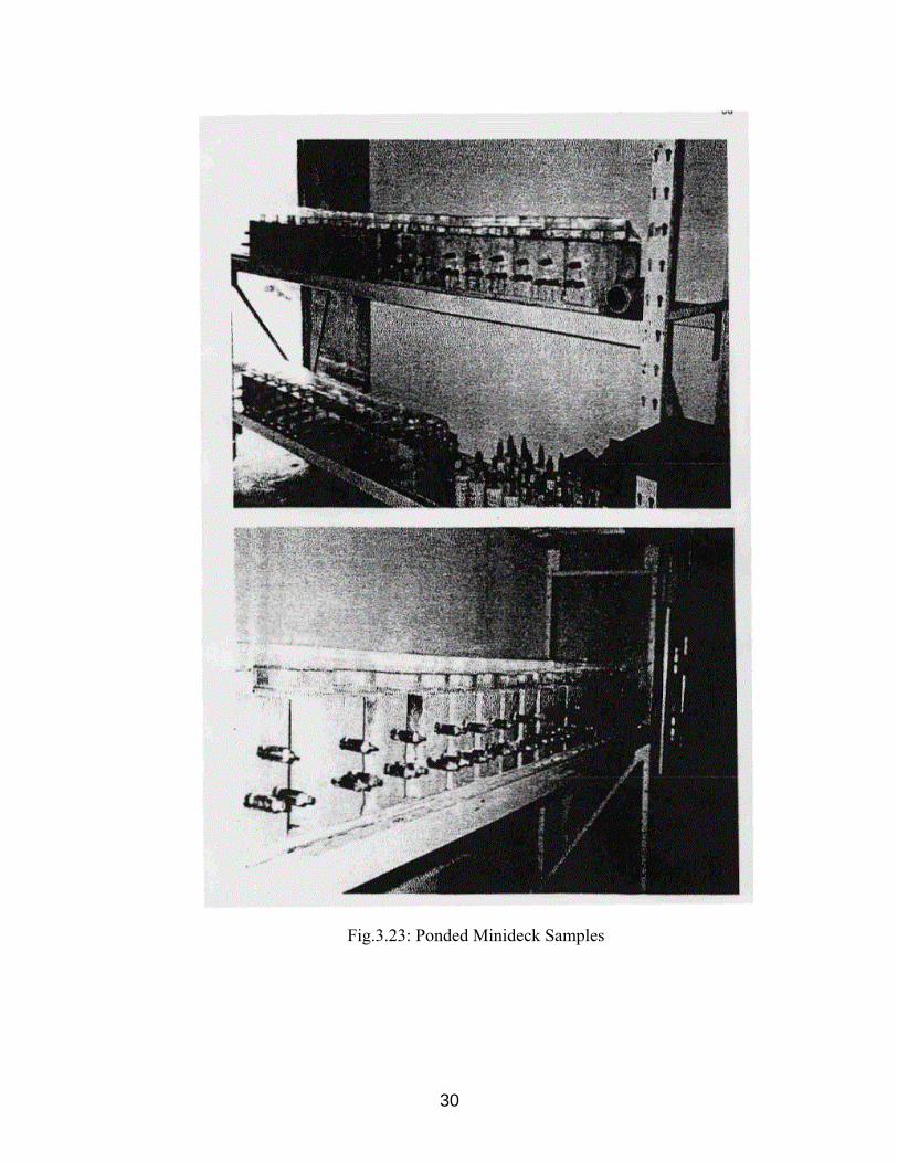
The samples were ponded with 3% NaCl solution and tested for corrosion rate
and corrosion potential as per ASTM G 109 and ASTM C 876, respectively. The ponded
specimens can be seen in Fig. 3.23. The corrosion data in provided in the Results and
Discussion Chapter.

29
Fig. 3.22: View of Plexiglas Dam
30
Fig.3.23: Ponded Minideck Samples
31
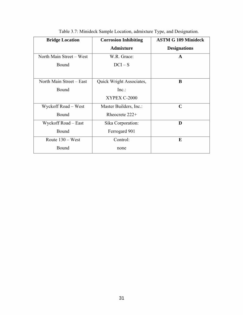
Table 3.7: Minideck Sample Location, admixture Type, and Designation.
Bridge Location Corrosion Inhibiting
Admixture
ASTM G 109 Minideck
Designations
North Main Street – West
Bound
W.R. Grace:
DCI – S
A
North Main Street – East
Bound
Quick Wright Associates,
Inc.:
XYPEX C-2000
B
Wyckoff Road – West
Bound
Master Builders, Inc.:
Rheocrete 222+
C
Wyckoff Road – East
Bound
Sika Corporation:
Ferrogard 901
D
Route 130 – West
Bound
Control:
none
E
32
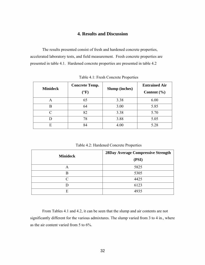
4. Results and Discussion
The results presented consist of fresh and hardened concrete properties,
accelerated laboratory tests, and field measurement. Fresh concrete properties are
presented in table 4.1. Hardened concrete properties are presented in table 4.2
Table 4.1: Fresh Concrete Properties
Minideck Concrete Temp.
(°F) Slump (inches)
Entrained Air
Content (%)
A 65 3.38 6.00 B 64 3.00 5.85 C 82 3.38 5.70 D 78 3.88 5.05 E 84 4.00 5.28
Table 4.2: Hardened Concrete Properties
Minideck 28Day Average Compressive Strength
(PSI)
A 5825 B 5305 C 4425 D 6123 E 4935
From Tables 4.1 and 4.2, it can be seen that the slump and air contents are not
significantly different for the various admixtures. The slump varied from 3 to 4 in., where
as the air content varied from 5 to 6%.
33
Compressive strength varied from 4425 to 6125 psi. The variation could be
considered a little high. However, this variation may not influence corrosion studies
because the corrosion is primarily influenced by permeability. Rapid air permeability
tests indicate that the variation in permeability among the five bridge decks is not
significant.
Corrosion rate and corrosion potential for minidecks subjected to accelerated
corrosion and actual bridge decks are presented in the following sections. Since the
corrosion process did not start in either set of samples, a correlation could not be
developed. However the data will be very useful if future readings taken in the field
indicate corrosion activity. Once corrosion activity is evident in the laboratory or field
tests, a correlation can be attempted.
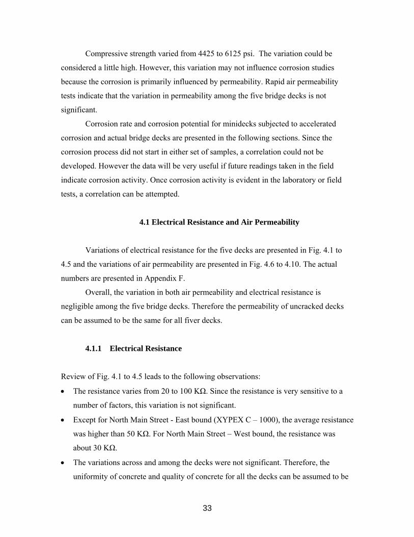
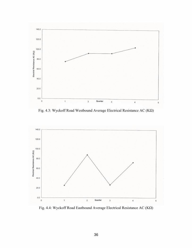
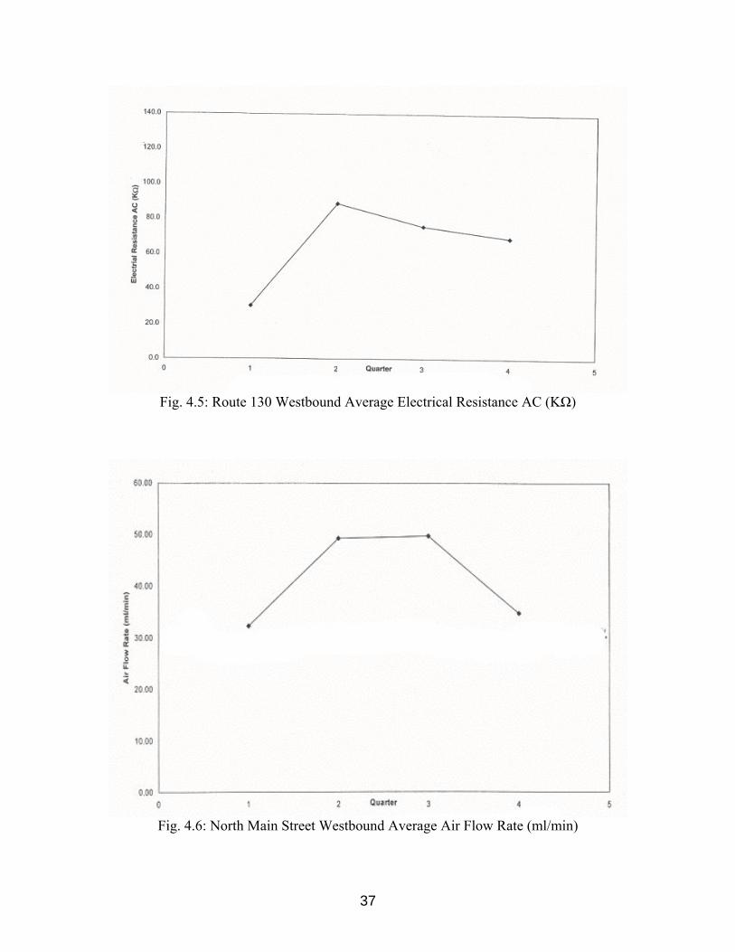
4.1 Electrical Resistance and Air Permeability
Variations of electrical resistance for the five decks are presented in Fig. 4.1 to
4.5 and the variations of air permeability are presented in Fig. 4.6 to 4.10. The actual
numbers are presented in Appendix F.
Overall, the variation in both air permeability and electrical resistance is
negligible among the five bridge decks. Therefore the permeability of uncracked decks
can be assumed to be the same for all fiver decks.
4.1.1 Electrical Resistance
Review of Fig. 4.1 to 4.5 leads to the following observations:
• The resistance varies from 20 to 100 KΩ. Since the resistance is very sensitive to a
number of factors, this variation is not significant.
• Except for North Main Street - East bound (XYPEX C – 1000), the average resistance
was higher than 50 KΩ. For North Main Street – West bound, the resistance was
about 30 KΩ.
• The variations across and among the decks were not significant. Therefore, the
uniformity of concrete and quality of concrete for all the decks can be assumed to be

34
same for all the five bridge decks. It should be noted that this observation is based on
the measurements taken on uncracked decks.
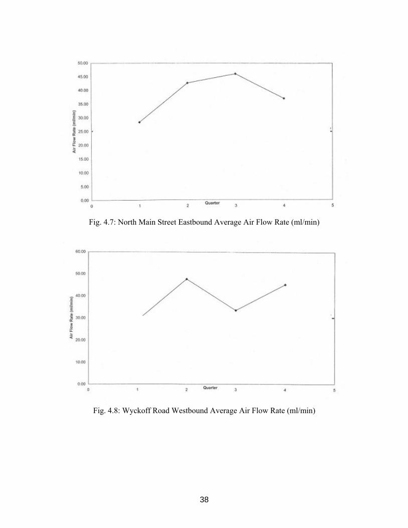
4.1.2 Air Permeability
Review of Fig 4.6 to 4.10 leads to the following observations:
• The air flow rate varied from 25 to 45 ml/min.
• The magnitude of variation in air flow across and among (the five) the decks were
smaller for air flow as compared to electrical resistance. This should be expected
because air flow is primarily influenced by density. Other factors such as degree of
saturation have much less effect on permeability as compared to electrical resistance.
• Careful review of all the readings leads to the conclusion that the variation of air
permeability across and among the five decks is negligible. Here again, the results
were obtained on uncracked decks.

35
Fig. 4.1: North Main Street Westbound Average Electrical Resistance AC (KΩ)
Fig. 4.2: North Main Street Eastbound Average Electrical Resistance AC (KΩ)
36
Fig. 4.3: Wyckoff Road Westbound Average Electrical Resistance AC (KΩ)
Fig. 4.4: Wyckoff Road Eastbound Average Electrical Resistance AC (KΩ)
37
Fig. 4.5: Route 130 Westbound Average Electrical Resistance AC (KΩ)
Fig. 4.6: North Main Street Westbound Average Air Flow Rate (ml/min)
38
Fig. 4.7: North Main Street Eastbound Average Air Flow Rate (ml/min)
Fig. 4.8: Wyckoff Road Westbound Average Air Flow Rate (ml/min)

39
Fig. 4.9: Wyckoff Road Westbound Average Air Flow Rate (ml/min)
Fig. 4.10: Route 130 Westbound Average Air Flow Rate (ml/min)

40
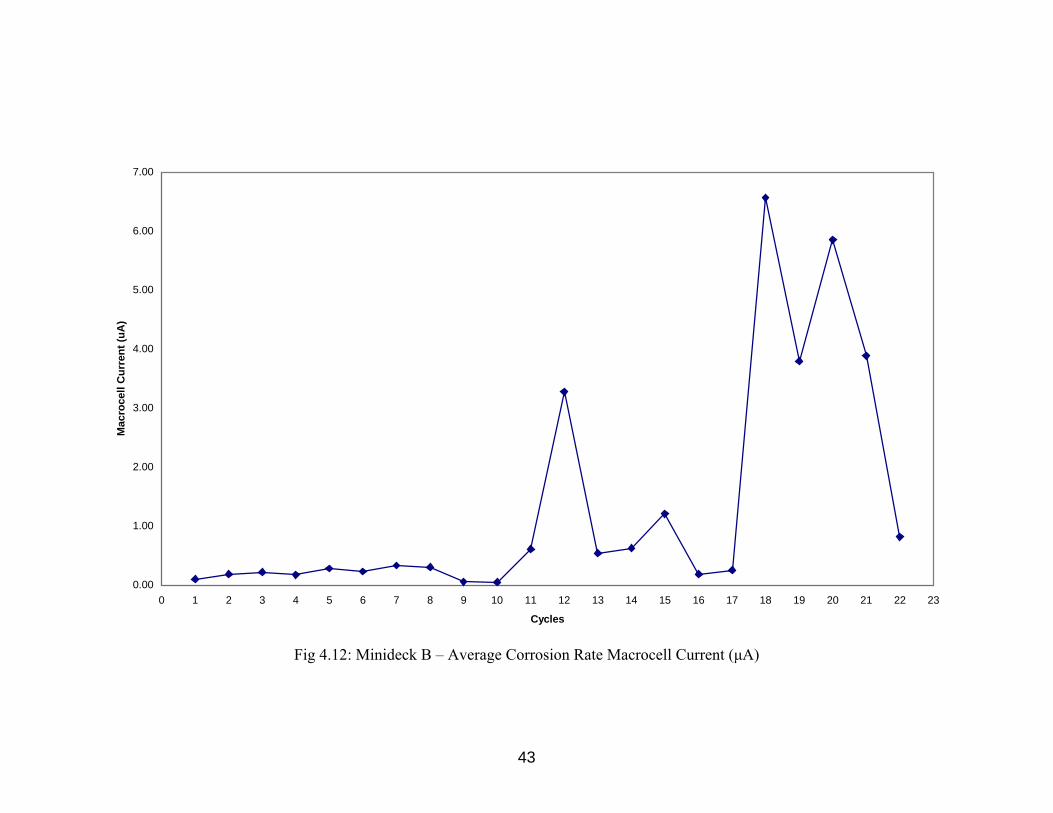
4.2 Corrosion Measurements
Corrosion potential and corrosion rate (ASTM G109) were made on both
minidecks and the five bridge decks. For minidecks, each cycle consists of two weeks of
ponding with salt water and two weeks of drying. For the bridge decks, measurements
were taken at approximately 6 months intervals. Since the corrosion rates were more
consistent, the changes in corrosion rate with number of cycles are presented in a
graphical form. The actual corrosion rates, corrosion potentials and variation of corrosion
potentials are presented in Appendix G.
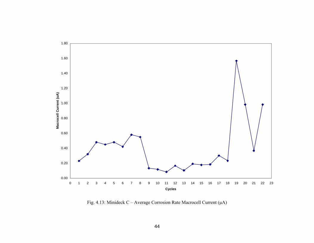
The variations of corrosion rate for minidecks are presented in Fig. 4.11 to 4.15.
The results for decks with W.R. Grace (DCI – S), Quick Wright Associates Inc.
(XYPEX C-2000), Master Builders, INC (Rheocrete 222+) and Sika Corporation
(Ferrogard 901) are presented is Fig. 4.11, 4.12, 4.13 and 4.14 respectively. The results
for the control deck with no inhibitors are presented in Fig. 4.15.
The variation of corrosion rate measured on actual decks is presented in Fig. 4.16
to 4.10. The results The results for decks with W.R. Grace (DCI – S), Quick Wright
Associates Inc. (XYPEX C-2000), Master Builders, INC (Rheocrete 222+) and Sika
Corporation (Ferrogard 901) are presented is Fig. 4.16, 4.17, 4.18 and 4.19 respectively.
The results for the control deck with no inhibitors are presented in Fig. 4.20.
A careful review of Fig. 4.11 to 4.20 and results presented in Appendix G lead to
the following observations:
• As expected, the variation of corrosion potential and corrosion rate is smaller in
bridge decks as compared to minidecks. This should be expected because the
corrosion potential on actual decks is non existent and minidecks were ponded
with salt solution.
• Corrosion activity is much lower in actual decks as compared to mini decks. For
example, the corrosion rate for actual decks is well bellow 1 µA where as for

41
minidecks the values are as high as 6 µA. Here again, the presence of salt solution
on minidecks plays an important role.
• There should not be any corrosion activity in the well constructed bridge decks
for at least 15 years, and the very low readings confirm the early trend.
• For minidecks, the corrosion rate has to be more than 10 µA in order to ascertain
the presence of corrosion. Unfortunately, none of the minidecks had average
readings more than 7 µA. Most readings were less than 2 µA and hence
conclusions could not be drawn on the actual or comparative performance of the
four corrosion inhibitors. Some of the decks are beginning to show some
corrosion activity. However, it was decided to terminate the rest program because
the decks were evaluated for more than 2 years.
• Further analysis of corrosion activities are presented in section 4.3.

42
0.00
1.00
2.00
3.00
4.00
5.00
6.00
0 1 2 3 4 5 6 7 8 9 10 11 12 13 14 15 16 17 18 19 20 21 22 23
Cycles
Mac
roce
ll C
urre
nt (u
A)
Fig 4.11: Minideck A – Average Corrosion Rate Macrocell Current (µA)
43
0.00
1.00
2.00
3.00
4.00
5.00
6.00
7.00
0 1 2 3 4 5 6 7 8 9 10 11 12 13 14 15 16 17 18 19 20 21 22 23
Cycles
Mac
roce
ll C
urre
nt (u
A)
Fig 4.12: Minideck B – Average Corrosion Rate Macrocell Current (µA)
44
0.00
0.20
0.40
0.60
0.80
1.00
1.20
1.40
1.60
1.80
0 1 2 3 4 5 6 7 8 9 10 11 12 13 14 15 16 17 18 19 20 21 22 23
Cycles
Mac
roce
ll C
urre
nt (u
A)
Fig. 4.13: Minideck C – Average Corrosion Rate Macrocell Current (µA)
45
0.00
0.20
0.40
0.60
0.80
1.00
1.20
1.40
1.60
1.80
2.00
0 1 2 3 4 5 6 7 8 9 10 11 12 13 14 15 16 17 18 19 20 21 22 23
Cycles
Mac
roce
ll C
urre
nt (u
A)
Fig 4.14: Minideck D – Average Corrosion Rate Macrocell Current (µA)

46
0.00
0.50
1.00
1.50
2.00
2.50
3.00
3.50
0 1 2 3 4 5 6 7 8 9 10 11 12 13 14 15 16 17 18 19 20 21 22 23
Cycles
Mac
roce
ll C
urre
nt (u
A)
Fig. 4.15: Minideck E – Average Corrosion Rate Macrocell Current (µA)

47
0.00
0.20
0.40
0.60
0.80
1.00
1.20
1.40
1.60
1.80
2.00
Cycle 1 Cycle 2 Cycle 3 Cycle 4 Cycle 5 Cycle 6 Cycle 7 Cycle 8Cycles
Cor
rosi
on R
ate
Mac
roce
ll C
urre
nt (u
A)
Fig 4.16: North Main Street Westbound GECOR 6 Average Corrosion Rate Macrocell Current (µA)
48
0
0.2
0.4
0.6
0.8
1
1.2
1.4
1.6
1.8
2
Cycle 1 Cycle 2 Cycle 3 Cycle 4 Cycle 5 Cycle 6 Cycle 7 Cycle 8
Cycle
Cor
rosi
on R
ate
Mac
roce
ll C
urre
nt (u
A)
Fig. 4.17: North Main Street Eastbound Average Corrosion Rate Macrocell Current (µA)

49
0.00
0.20
0.40
0.60
0.80
1.00
1.20
1.40
1.60
1.80
2.00
Cycle 1 Cycle 2 Cycle 3 Cycle 4 Cycle 5 Cycle 6 Cycle 7 Cycle 8
Cycles
Cor
rosi
on R
ate
Mac
roce
ll C
urre
nt (u
A)
Fig 4.18: Wyckoff Road Westbound GECOR 6 Average Corrosion Rate Macrocell Current (µA)
50
0.00
0.20
0.40
0.60
0.80
1.00
1.20
1.40
1.60
1.80
2.00
Cycle 1 Cycle 2 Cycle 3 Cycle 4 Cycle 5 Cycle 6 Cycle 7 Cycle 8
Cycles
Cor
rosi
on R
ate
Mac
roce
ll C
urre
nt
Fig 4.19: Wyckoff Road Eastbound GECOR 6 Average Corrosion Rate Macrocell Current (µA)
51
0.00
0.20
0.40
0.60
0.80
1.00
1.20
1.40
1.60
1.80
2.00
Cycle 1 Cycle 2 Cycle 3 Cycle 4 Cycle 5 Cycle 6 Cycle 7 Cycle 8
Cycles
Cor
rosi
on R
ate
Mar
ocel
l Cur
rent
(uA
)
Fig 4.20: Route 130 Westbound GECOR 6 Average Corrosion Rate Macrocell Current (µA)
52
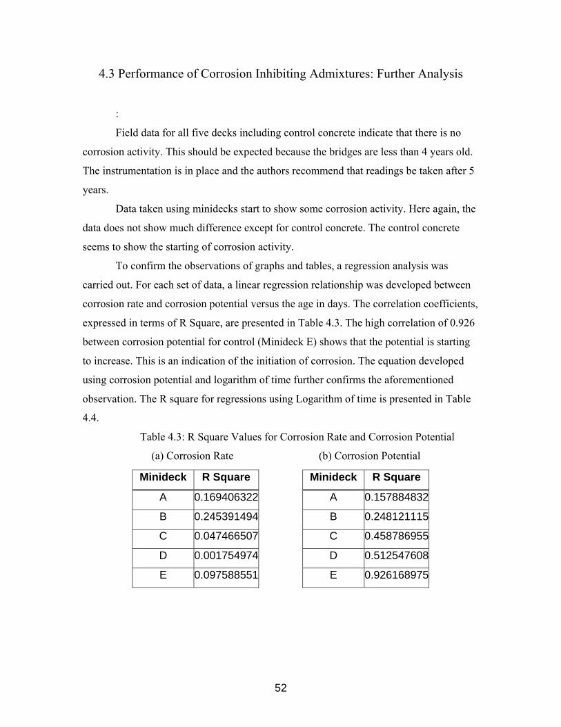
4.3 Performance of Corrosion Inhibiting Admixtures: Further Analysis
:
Field data for all five decks including control concrete indicate that there is no
corrosion activity. This should be expected because the bridges are less than 4 years old.
The instrumentation is in place and the authors recommend that readings be taken after 5
years.
Data taken using minidecks start to show some corrosion activity. Here again, the
data does not show much difference except for control concrete. The control concrete
seems to show the starting of corrosion activity.
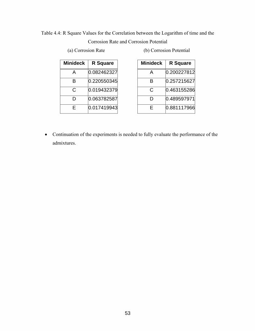
To confirm the observations of graphs and tables, a regression analysis was
carried out. For each set of data, a linear regression relationship was developed between
corrosion rate and corrosion potential versus the age in days. The correlation coefficients,
expressed in terms of R Square, are presented in Table 4.3. The high correlation of 0.926
between corrosion potential for control (Minideck E) shows that the potential is starting
to increase. This is an indication of the initiation of corrosion. The equation developed
using corrosion potential and logarithm of time further confirms the aforementioned
observation. The R square for regressions using Logarithm of time is presented in Table
4.4.
Table 4.3: R Square Values for Corrosion Rate and Corrosion Potential
(a) Corrosion Rate (b) Corrosion Potential
Minideck R Square Minideck R Square
A 0.169406322 A 0.157884832
B 0.245391494 B 0.248121115
C 0.047466507 C 0.458786955
D 0.001754974 D 0.512547608
E 0.097588551 E 0.926168975
53
Table 4.4: R Square Values for the Correlation between the Logarithm of time and the
Corrosion Rate and Corrosion Potential
(a) Corrosion Rate (b) Corrosion Potential
• Continuation of the experiments is needed to fully evaluate the performance of the
admixtures.
Minideck R Square Minideck R Square
A 0.082462327 A 0.200227812
B 0.220550345 B 0.257215627
C 0.019432379 C 0.463155286
D 0.063782587 D 0.489597971
E 0.017419943 E 0.881117966
54
5. Conclusions and Recommendations
5.1 Conclusions
Based on the experimental results and observations made during the fabrication
and testing, the following conclusions can be drawn:
• There are no significant differences in the plastic and hardened concrete
properties for the four admixtures evaluated.
• The authors suggest that though the results of the Surface Air Flow Field
Permeability Indicator can be used for a rough evaluation and comparison of
admixtures, it should not be used as an accurate means to determine air
permeability.
• In authors’ opinion, the GECOR 6 Corrosion Rate Meter provides better electrical
resistance reading than the Electrical Resistance Test of Penetrating Sealers.
• Time of exposure is not sufficient to cause any corrosion activity in the field. This
is reflected in the corrosion potential and corrosion rate readings taken in the
field. If the instrumentation is protected readings could be taken after 15 or 20
years of exposure.
• As expected, the laboratory samples had more corrosion activity. However, here
again, the corrosion was not sufficient to evaluate the difference in behavior
among various admixtures. Since the samples are not cracked, admixtures that
decrease the permeability show less corrosion activity. However, the difference is
not statistically different. The control mix is starting to show some corrosion
activity. This lack of corrosion activity denied the achievement of the objective of
“evaluation of the effectiveness of the admixtures.”
5.2 Recommendations
Based on the scientific principles and comparative behavior of mini decks, the
authors recommend the use of XYPEX in decks with no cracks. The admixture provides
a more dense and impermeable concrete that reduces the ingress of chemicals.
55
The aforementioned statement is not intended to indicate that only XYPEX is
recommended for use. The remaining three admixtures are being used in the field. Since
we could not initiate the corrosion in any of the minidecks, we are not able to provide any
recommendations on the contribution of inhibitors. Since the quality of concrete and
quality control were good, the control concrete itself provided very good performance.
Even though this is good and logical, the primary objective of the research could not be
fulfilled. Since the experiments were run for more than 2 years, the NJDOT decided to
terminate the project.
For field study, the authors strongly recommend to continue the measurements of
corrosion potential and corrosion rate. The instrumentation is in place and the results will
be very valuable for the entire world. It is recommended that the readings should be taken
every 6 months. Since the bridges are in use, NJDOT should provide traffic control
during measurements. Since the instrumentation is in place, the cost for the measurement
and yearly report could be in the range of $7,000. If the contract is extended to 10 years,
15 years data could be obtained for an additional cost of $70,000. The authors believe
that the uniqueness of this database, which does not exit anywhere, makes this
expenditure worthwhile.
For the laboratory study, improvements are needed for the current procedure. The
major problem was the permeability of concrete. The concrete should not be allowed to
dry-out and the corrosion should be induced after 24 hours. The authors recommend that
NJDOT initiate another study to develop the test procedure. The main factors that
contribute to corrosion are permeability of concrete and cracks through which the
chemicals permeate. The accelerated test method should be designed to incorporate these
two factors. The study should utilize 2 or 3 NJDOT standard mixes with no admixture.
However, for both sets of specimens, a higher water cement ratio should be used to
increase the permeability of concrete; In addition, the samples should not be cured,
resulting further increase in permeability.
The mini decks can be prepared using the same procedure used for the current
Minidecks. However, for one set of samples, very thin plastic plates should be placed on
both top and bottom covers to simulate cracking.

56
The objective of the new study is to develop an accelerated test method that will
provide corrosion within 18 months. The test method should be able to evaluate the
effectiveness of corrosion inhibitors. The envisioned variables are as follows:
• Minimum water-cement ratio that can provide corrosion in 18 months for the
NJDOT mixes.
• Maximum thickness of plates used for crack simulation.
The researchers can chose a range for both water-cement ratio and plate thickness to
formulate their experimental program.
57
6. References
1. ACI 222R-1996 Corrosion of Metals in Concrete, ACI Committee 222 American
Concrete Institute 1997
2. ASTM G 109, Annual Book of ASTM Standards
3. ASTM C 876, Annual Book of ASTM Standards
4. ASTM C 94, Annual Book of ASTM Standards
5. ASTM C 150, Annual Book of ASTM Standards
6. Beeby, A.W., Development of a Corrosion Cell for the study of the influences of the
environment and the Concrete; Fundamentals and Civil Engineering Practice, E & FN
Spoon, London, UK 1992
7. Bentur, A., Diamond, S., Burke, N.S., Modern Concrete Technology Steel Corrosion
in Concrete; Fundamentals and Civil Engineering Practice, E & FN Spoon, London,
UK 1992
8. Berke, N.S., Hicks, M.C., Hoopes, R.J., Concrete Bridges in Aggressive
Environments, “SP-151-3 Condition Assessment of Field Structures with Calcium
Nitrate”, American Concrete Institute 1995
9. Berke, N.S., Roberts, L.R. Concrete Bridges in Aggressive Environments, “SP 119-
20 Use of Concrete Admixtures to provide Long-Term Durability from Steel
Corrosion”, American Concrete Institute 1995
10. Berke, N.S., Weil, T.G., Advances in Concrete Technology, “World-Wide Review of
Corrosion Inhibitors in Concrete” Published by CNMET, Canada 1997
11. Broomfield, John P., Corrosion of Steel in Concrete: Understanding Investigation and
Repair, E & FN Spoon, London, UK 1997
58
12. DCI – S Corrosion Inhibitor, W.R. Grace and Co. 1997 http:///www.gcp-
grace.com/products/concrete/summaries/dcis.html and http://www.gcp-
grace/pressroom/adva_nz.html
13. MacDonald, M., Sika Ferrogard 901 and 903 Corrosion Inhibitors: Evaluation of test
Program, Special Services Division, Sika Corporation 1996
14. Manual for the operation of a surface Air Flow Field Permeability Indicator, Texas
Research Institute Austin, Inc., Austin Texas, June 1994
15. Page, C.L., Treadway, K.W.J., Bamforth. P.B., Corrosion of Reinforcement in
Concrete Society of the chemical Industry, Symposium held at Warwickshire, UK
1990
16. Rheocrete 222+: Organic Corrosion Inhibiting Admixture, Master Builders, Inc.
Printed in USA 1995
17. Scannel, William T. Participant’s Workbook: FHWA – SHRP Showcase, U.S.
Department of Transportation, Conncorr Inc., Ashburn Virginia, July, 1996
18. Sennour, M.L., Wheat, H.G., Carrasquillo, R.L., The effects of chemical and Mineral
Admixtures on the Corrosion of Steel in Concrete, University of Texas, Austin 1994
19. XYPEX Concrete Waterproofing by Crystallization, Quick-Wright Associates, Ink.
http://www.qwa.com/concrete.html
59
Appendix A
Description of Equipment and Test Procedure for GECOR 6
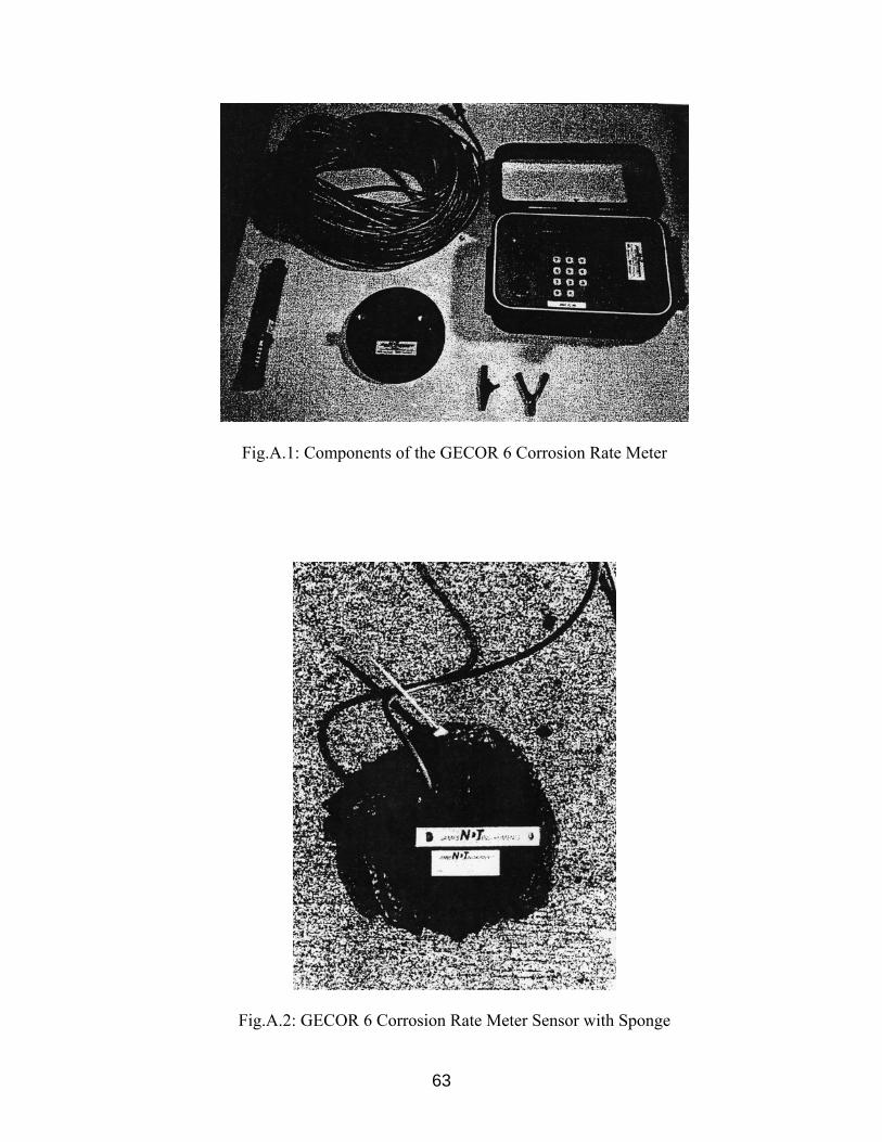
The GECOR 6 Corrosion Rate Meter has three major components, the rate meter and two
separate sensors. Only the larger sensor was used during this project. The sensor is filled
with a saturated Cu/CuSO4 solution for the test for half-cell potential. The main
components of this device can be seen in Fig.A.1. A wet sponge is used between the
probe and the concrete surface as seen in Fig. A.2. Long Lengths of wire are also
provided to connect the sensor to the rate meter and to connect the rate meter to the
reinforcing bar mat of the bridge deck, a necessary step for the operation of the meter.
The procedure for the operation of the GECOR 6 Corrosion Rate Meter is as
follows (Scannel, 1996):
1. The device should not be operated at temperatures below 0°C (32°°F) or above 50 C
(122°F). The relative humidity within the unit should not exceed 80%.
2. Use a reinforcing steel locator to define the layout at the test location. Mark the bar
pattern on the concrete surface at the test location.
3. Place a wet sponge and the sensor over a single bar or over the point where the bars
intersect perpendicularly if the diameter of both bars is known.
4. Connect the appropriate lead to an exposed bar. The leads from the sensor and
exposed reinforcing steel are then connected to the GECOR device.
5. Turn on the unit. The program version appears on the display screen.
“LG-ECM-06 V2.0
© GEOCISA 1993”
60
6. A help message appears on the screen momentarily. This message advises the
operator to use the arrows for selecting an option and C.R. to activate an option. The
various options are:
• “CORROSION RATE MEASUREMENT”
• “REL.HUMIDITY AND TEMPERATURE”
• “RESISTIVITY MEASUREMENT PARAMETERS”
• “EDIT MEASUREMENT PARAMETERS”
• “DATAFILE SYSTEM EDITING”
• “DATAAND TIME CONTROL”
7. Select the option CORROSION RATE MEASUREMENT and press the C.R. key.
8. The screen prompts the user to input the area of steel. Calculate the area of steel
using the relationship, Area = 3.142 x D x 10.5 cm. D is the diameter of the bar in
centimeters and 10.5 cm. (4 in.) is the length of the bar confined by the guard ring.
Key ii the area to one decimal space. In case of an error, use the B key to delete the
previous character. Press the C.R. key to enter the area.
9. The next screen displays;
“ADJUSTING
OFFSET, WAIT”
No operator input is required at this stage. The meter measures the half-cell potential and
then nulls it out to measure the potential shift created by the current applied from the
sensor.
10. The next screen displays:
“Er mV OK”
“Vs mV OK”
Er (ECORR) is the static half-cell potential versus CSE and Vs is the difference in
potential between the reference electrodes, which control the current confinement.
Once the Er and the Vs values are displayed, no input is required from the operator.

61
11. The meter now calculates the optimum applied current ICE. This current is applied
through the counter electrode at the final stage of the measurement. The optimum ICE
value is displayed. No input is required from the operator.
12. The next screen displays the polarized potential values. No input is required from the
operator.
13. The meter now calculates the “balance constant” in order to apply the correct current
to the guard ring. It is displayed on the next screen. No input is required from the
operator.
14. The meter now calculated the corrosion rate using the data collected from the sensor
and input from the operator. The corrosion rate is displayed in µA/cm2. Associated
parameters including corrosion potential, mV and electrical resistance KΏ can be
viewed using the cursor keys.
15. Record the corrosion rate, corrosion potential, electrical resistance.
16. Press the B key to reset the meter for the next reading. The screen will return to
CORROSION RATE MEASUREMENT. Repeat the procedure for the next test
location.
The corrosion rate and corrosion potential data can be interpreted using Table A.1 and
A.2 and Tables B.1 and B.2 in Appendix B, respectively. Higher resistance is an
indication for less potential for corrosion in the embedded steel due to higher density of
the concrete. Higher resistance is also an indication of improved insulation against the
electrochemical process of corrosion.
Unlike The Electrical Resistance Test for Penetrating Sealers, the GECOR 6 penetrates
the concrete surface for a greater area of measurement.
62
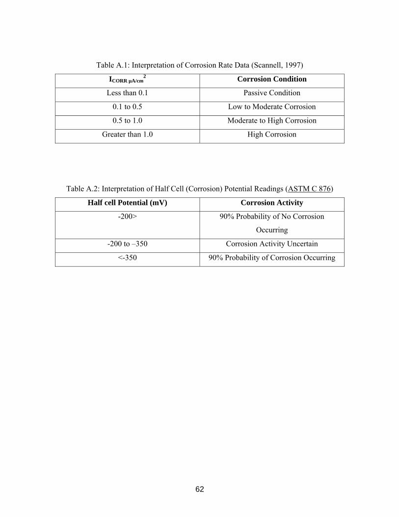
Table A.1: Interpretation of Corrosion Rate Data (Scannell, 1997)
ICORR µA/cm2 Corrosion Condition
Less than 0.1 Passive Condition
0.1 to 0.5 Low to Moderate Corrosion
0.5 to 1.0 Moderate to High Corrosion
Greater than 1.0 High Corrosion
Table A.2: Interpretation of Half Cell (Corrosion) Potential Readings (ASTM C 876)
Half cell Potential (mV) Corrosion Activity
-200> 90% Probability of No Corrosion
Occurring
-200 to –350 Corrosion Activity Uncertain
<-350 90% Probability of Corrosion Occurring
63
Fig.A.1: Components of the GECOR 6 Corrosion Rate Meter
Fig.A.2: GECOR 6 Corrosion Rate Meter Sensor with Sponge
64
Appendix B
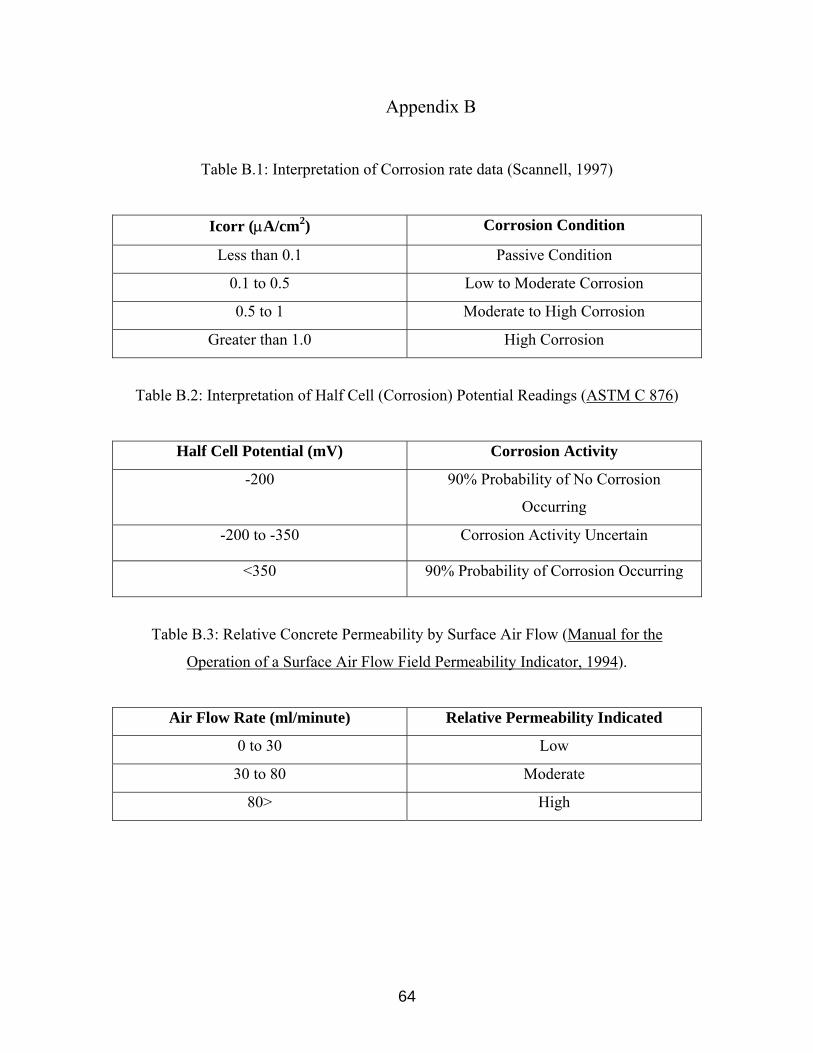
Table B.1: Interpretation of Corrosion rate data (Scannell, 1997)
Icorr (µA/cm2) Corrosion Condition
Less than 0.1 Passive Condition
0.1 to 0.5 Low to Moderate Corrosion
0.5 to 1 Moderate to High Corrosion
Greater than 1.0 High Corrosion
Table B.2: Interpretation of Half Cell (Corrosion) Potential Readings (ASTM C 876)
Half Cell Potential (mV) Corrosion Activity
-200 90% Probability of No Corrosion
Occurring
-200 to -350 Corrosion Activity Uncertain
<350 90% Probability of Corrosion Occurring
Table B.3: Relative Concrete Permeability by Surface Air Flow (Manual for the
Operation of a Surface Air Flow Field Permeability Indicator, 1994).
Air Flow Rate (ml/minute) Relative Permeability Indicated
0 to 30 Low
30 to 80 Moderate
80> High

65
Appendix C
Description of the Equipment and the Test Procedure for the Surface Air Flow
Field Permeability Indicator
A picture of the device and its accessories can be seen in Fig.C.1 and Fig.C.2. For
transportability the device uses a rechargeable NI-Cad battery. The suction foot is
mounted using three centering springs to allow it to rotate and swivel in relation to the
main body. A closed cell foam gasket is used between the foot and the testing surface to
create an airtight seal. Two-foot pads are threaded into the suction foot so the operator
can apply pressure to compress the gasket. The switches to open the solenoid and hold
the current reading are located within easy reach at the base of the handles. Digital
displays for the permeability readings and the time are located at the top of the device
Fig.C.3. Outline drawings of the device and its schematics can be seen on Fig.C.4 and
Fig.C.5, respectively (Manual for the Operation of a Surface Air Flow Field Permeability
Indicator, 1994).
Fig.C.1: Surface Air Flow Field Permeability Indicator (Front View)
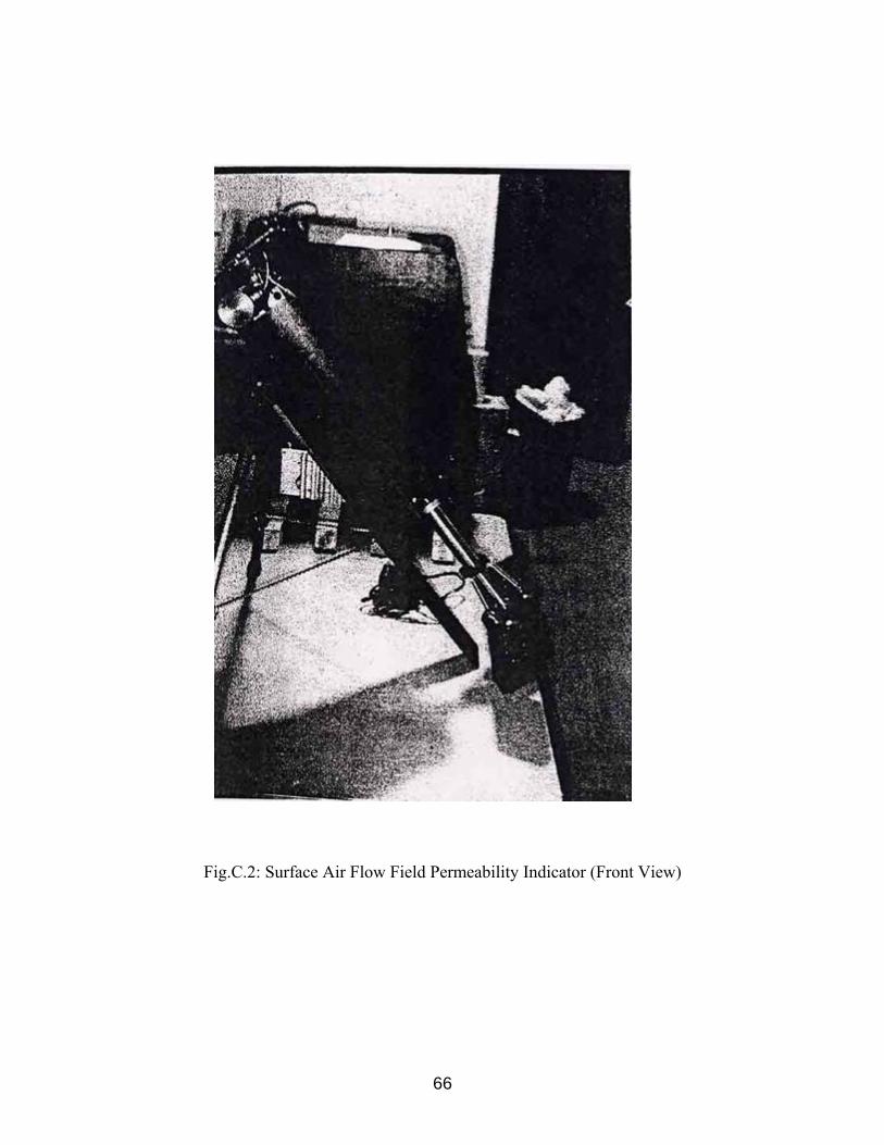
66
Fig.C.2: Surface Air Flow Field Permeability Indicator (Front View)

67
Fig.C.3: Surface Air Flow Field Permeability Indicator
(Top View of Digital Displays)
Fig.C.4: Drawing of Concrete Surface Air Flow Permeability Indicator
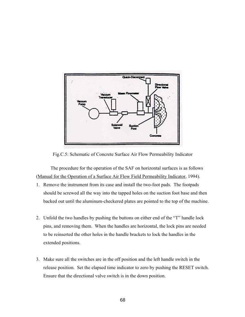
68
Fig.C.5: Schematic of Concrete Surface Air Flow Permeability Indicator
The procedure for the operation of the SAF on horizontal surfaces is as follows
(Manual for the Operation of a Surface Air Flow Field Permeability Indicator, 1994).
1. Remove the instrument from its case and install the two-foot pads. The footpads
should be screwed all the way into the tapped holes on the suction foot base and then
backed out until the aluminum-checkered plates are pointed to the top of the machine.
2. Unfold the two handles by pushing the buttons on either end of the “T” handle lock
pins, and removing them. When the handles are horizontal, the lock pins are needed
to be reinserted the other holes in the handle brackets to lock the handles in the
extended positions.
3. Make sure all the switches are in the off position and the left handle switch in the
release position. Set the elapsed time indicator to zero by pushing the RESET switch.
Ensure that the directional valve switch is in the down position.
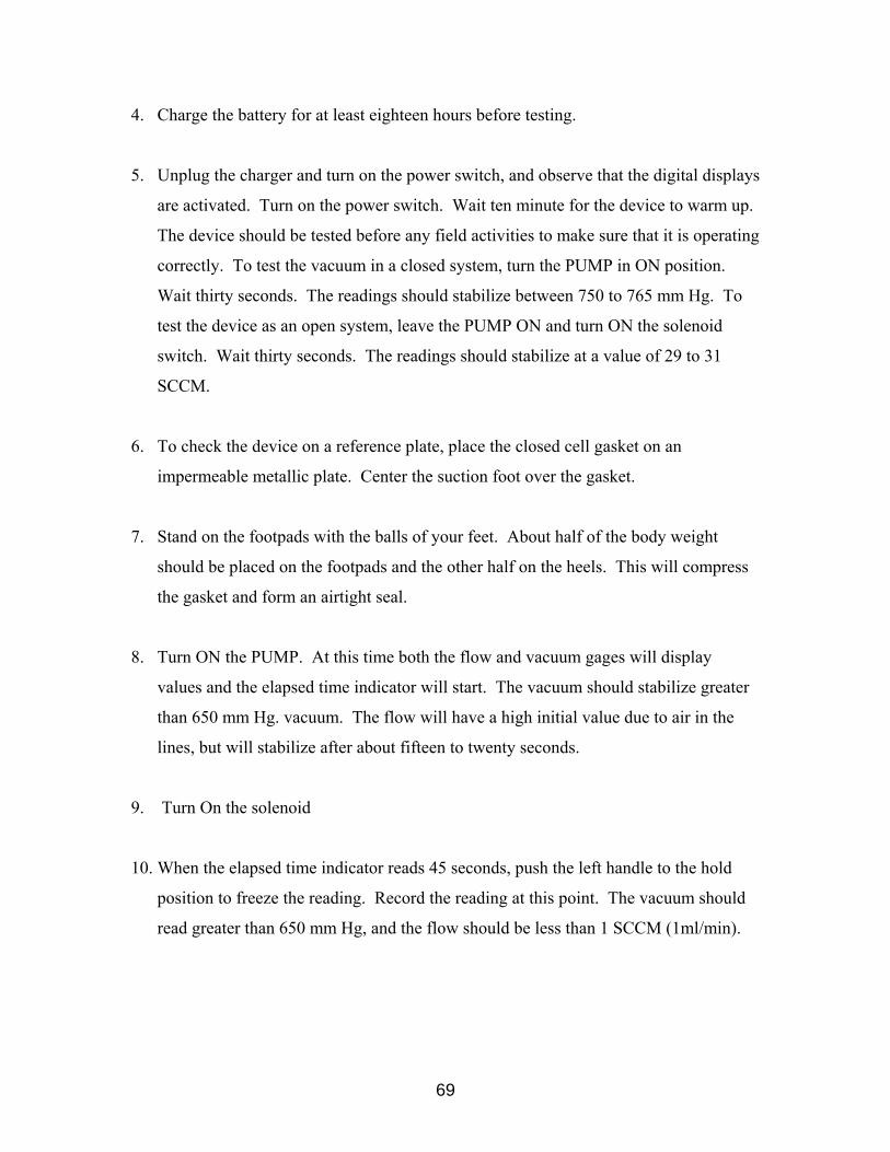
69
4. Charge the battery for at least eighteen hours before testing.
5. Unplug the charger and turn on the power switch, and observe that the digital displays
are activated. Turn on the power switch. Wait ten minute for the device to warm up.
The device should be tested before any field activities to make sure that it is operating
correctly. To test the vacuum in a closed system, turn the PUMP in ON position.
Wait thirty seconds. The readings should stabilize between 750 to 765 mm Hg. To
test the device as an open system, leave the PUMP ON and turn ON the solenoid
switch. Wait thirty seconds. The readings should stabilize at a value of 29 to 31
SCCM.
6. To check the device on a reference plate, place the closed cell gasket on an
impermeable metallic plate. Center the suction foot over the gasket.
7. Stand on the footpads with the balls of your feet. About half of the body weight
should be placed on the footpads and the other half on the heels. This will compress
the gasket and form an airtight seal.
8. Turn ON the PUMP. At this time both the flow and vacuum gages will display
values and the elapsed time indicator will start. The vacuum should stabilize greater
than 650 mm Hg. vacuum. The flow will have a high initial value due to air in the
lines, but will stabilize after about fifteen to twenty seconds.
9. Turn On the solenoid
10. When the elapsed time indicator reads 45 seconds, push the left handle to the hold
position to freeze the reading. Record the reading at this point. The vacuum should
read greater than 650 mm Hg, and the flow should be less than 1 SCCM (1ml/min).
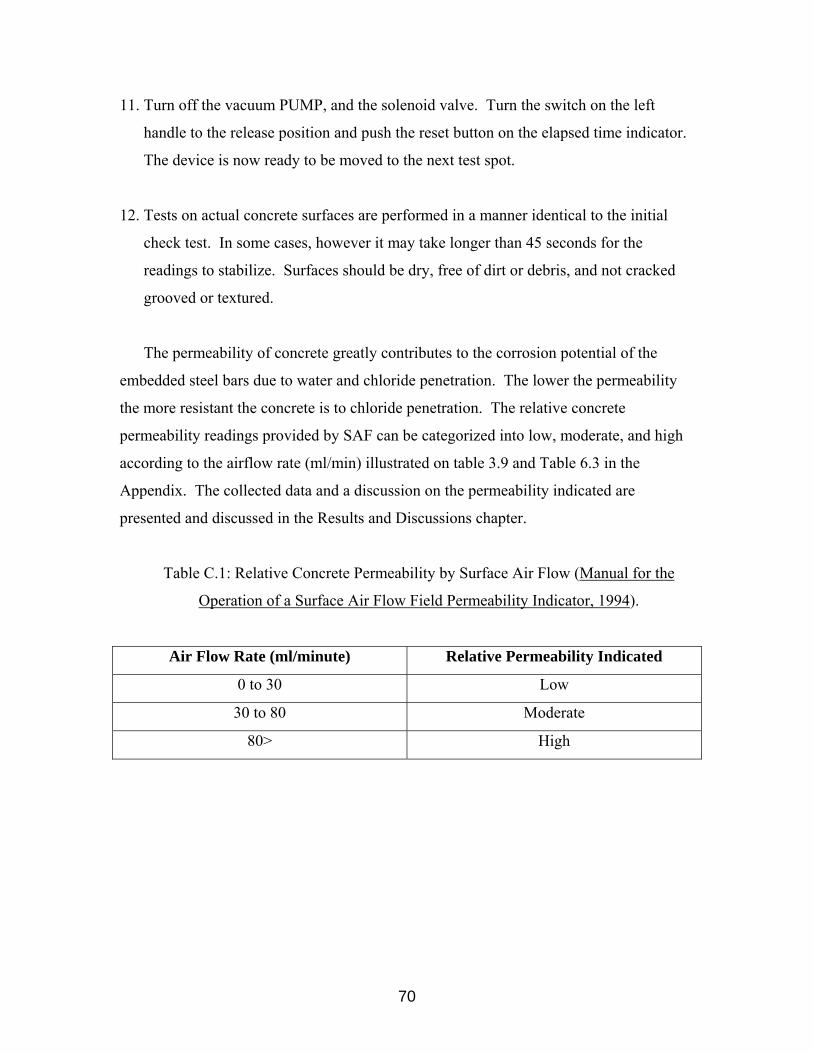
70
11. Turn off the vacuum PUMP, and the solenoid valve. Turn the switch on the left
handle to the release position and push the reset button on the elapsed time indicator.
The device is now ready to be moved to the next test spot.
12. Tests on actual concrete surfaces are performed in a manner identical to the initial
check test. In some cases, however it may take longer than 45 seconds for the
readings to stabilize. Surfaces should be dry, free of dirt or debris, and not cracked
grooved or textured.
The permeability of concrete greatly contributes to the corrosion potential of the
embedded steel bars due to water and chloride penetration. The lower the permeability
the more resistant the concrete is to chloride penetration. The relative concrete
permeability readings provided by SAF can be categorized into low, moderate, and high
according to the airflow rate (ml/min) illustrated on table 3.9 and Table 6.3 in the
Appendix. The collected data and a discussion on the permeability indicated are
presented and discussed in the Results and Discussions chapter.
Table C.1: Relative Concrete Permeability by Surface Air Flow (Manual for the
Operation of a Surface Air Flow Field Permeability Indicator, 1994).
Air Flow Rate (ml/minute) Relative Permeability Indicated
0 to 30 Low
30 to 80 Moderate
80> High

71
Appendix D
Description and Test Procedure for Resistance Measurement
The materials needed for this test are shown in Fig.D.1 and are as follows:
Fine line tape (1/8in. wide)
Metal mask (with 5/8in. wide and 4 in. long cutout)
Conductive silver spray paint
Duct tape
Nilsson 400, soil resistance meter
Multimeter
Thermometer
Infrared propane heater
Fig.D.1: Equipment Required for Electrical Resistance Test for Penetrating Sealers

72
The procedure for the performing the Electrical Resistance Test for Penetrating
Sealers is as follows (Scannell, 1996)
1. Surface must be clean and dry with no grooves or cracks.
2. Apply the fine line tape t the test area.
3. Center metal mask over fine line tape.
4. Duct tape mask in place.
5. Spray paint lengthwise over slit six times.
6. Heat surface with infrared heater for five minutes keeping the temperature at 120 F.
7. Repeat steps 5 and 6 two additional times.
8. Remove the mask and the fine line tape.
9. Measure DC end-to-end resistance of both sides of the gage using the multimeter and
records the readings.
10. Measure the DC resistance between the two sides of the gage using the multimeter
and record the reading.
11. Compare the DC readings for the end-to-end resistance as well and the one taken
between the two sides to the acceptance criteria in Table 3.10.
12. Lay wet sponge on gage and keep wet for five minutes.
13. Remove the sponge and press a folder paper towel against the gage for five seconds.
14. Gently wipe the gage with a crumpled paper towel in a lengthwise direction.
15. Place the probes on the soil resistance meter against the gage and record the AC
resistance reading.
73
Table D.1: Preliminary DC Testing of Gauge (Scannell, 1996)
Test Acceptance Criteria
End-to-End Resistance 5 to 15 Ω – Very Good
up to 125 Ω - Acceptable
Insulation Resistance
(Side-to-Side)
>20MΩ – Normal
> 5 MΩ – Acceptable

74
Appendix E
Details of Connections on Bridge Decks
The details of the connections are presented in Fig.E.1, E.2, E.3, E.4 and E.5. The cables
were passed through flexible steel conduits and into rain tight steel enclosure to protect
then from the elements and from possible tampering Fig.E.6, E.7, E.8, E.9 and E.10. A
reinforcing steel locator was not needed because locations of reinforcement and
connections were recorded before the placement of the concrete
Connections were observed during the placement of concrete and were tested
after the concrete had hardened to check for broken connections. Pictures of the
connections during concrete placement can be seen in Fig.E.11, E.12, and E.13. All
connections survived and remained intact.
Photographs of the five bride decks tested on the new Route 133 Hightstown Bypass can
be seen in Fig.E.14, E.15, E.16, E.17, and E.18.
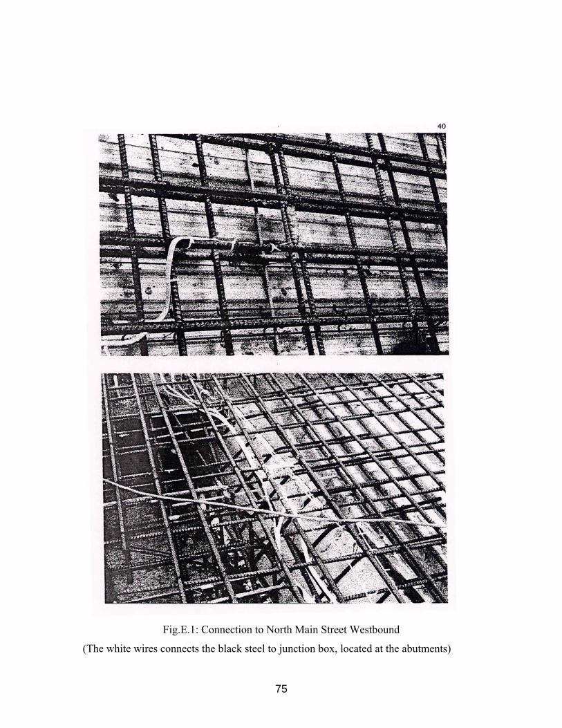
75
Fig.E.1: Connection to North Main Street Westbound
(The white wires connects the black steel to junction box, located at the abutments)
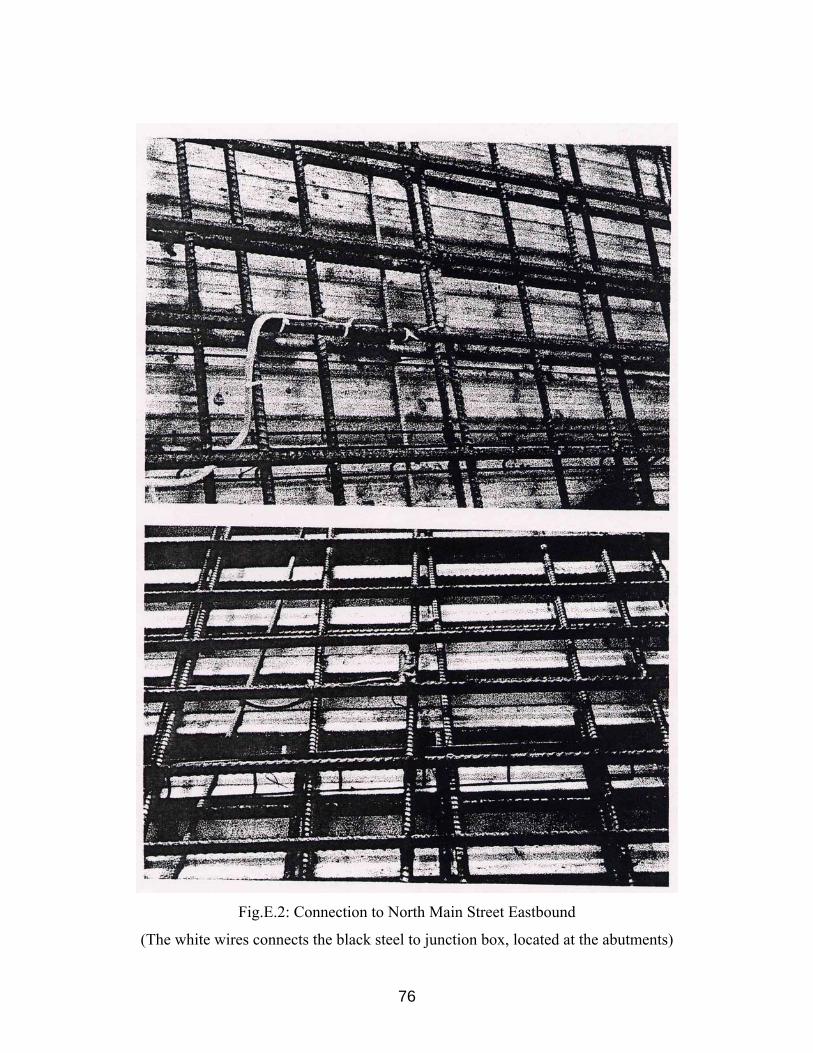
76
Fig.E.2: Connection to North Main Street Eastbound
(The white wires connects the black steel to junction box, located at the abutments)
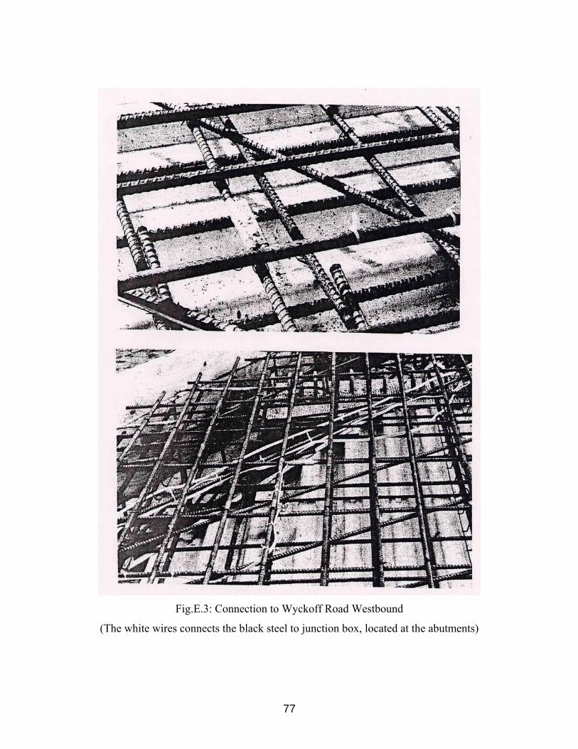
77
Fig.E.3: Connection to Wyckoff Road Westbound
(The white wires connects the black steel to junction box, located at the abutments)
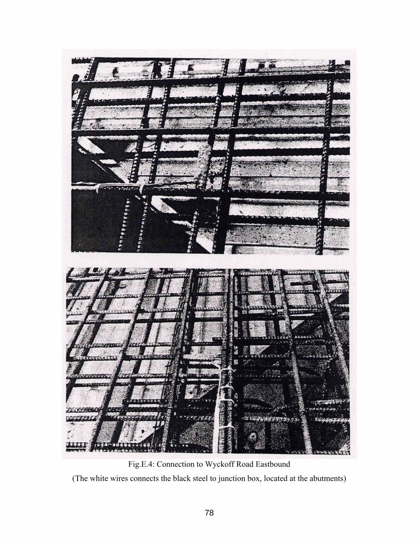
78
Fig.E.4: Connection to Wyckoff Road Eastbound
(The white wires connects the black steel to junction box, located at the abutments)

79
Fig.E.5: Connection to Route 130 Westbound
(The white wires connects the black steel to junction box, located at the abutments)

80
Fig.E.6: Conduits and Enclosure – North Main Street Westbound
Fig.E.7: Conduits and Enclosure – North Main Street Eastbound
(Junction box attached to the abutment)

81
Fig.E.8: Conduits and Enclosure – Wyckoff Road Westbound
Fig.E.9: Conduits and Enclosure – Wyckoff Road Eastbound
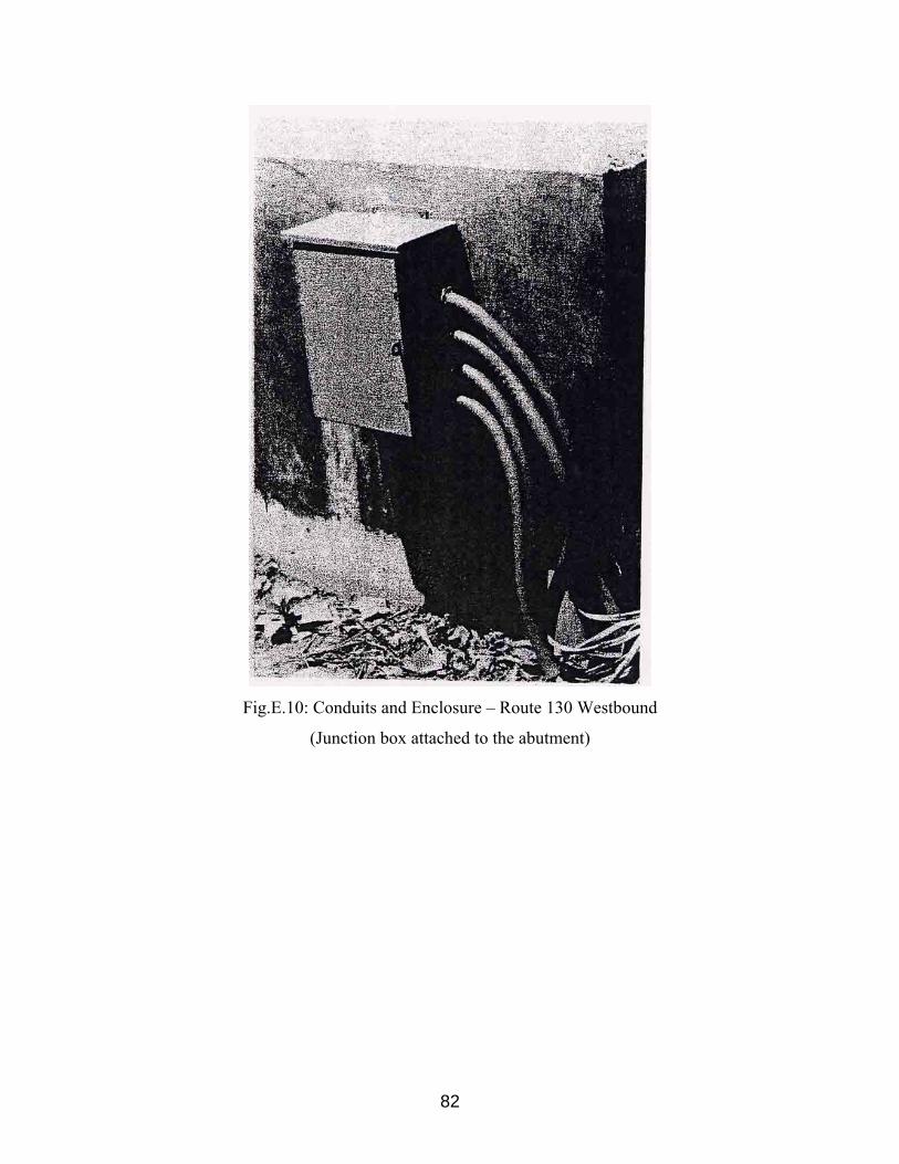
82
Fig.E.10: Conduits and Enclosure – Route 130 Westbound
(Junction box attached to the abutment)

83
Fig.E.11: Vibrating of Fresh Concrete at North Main Street Eastbound
Fig.E.12: Placement of Fresh Concrete at North Main Street Westbound
(Connections withstood the construction process)
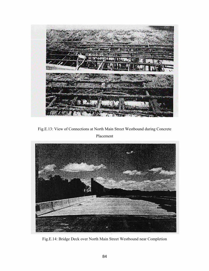
84
Fig.E.13: View of Connections at North Main Street Westbound during Concrete
Placement
Fig.E.14: Bridge Deck over North Main Street Westbound near Completion
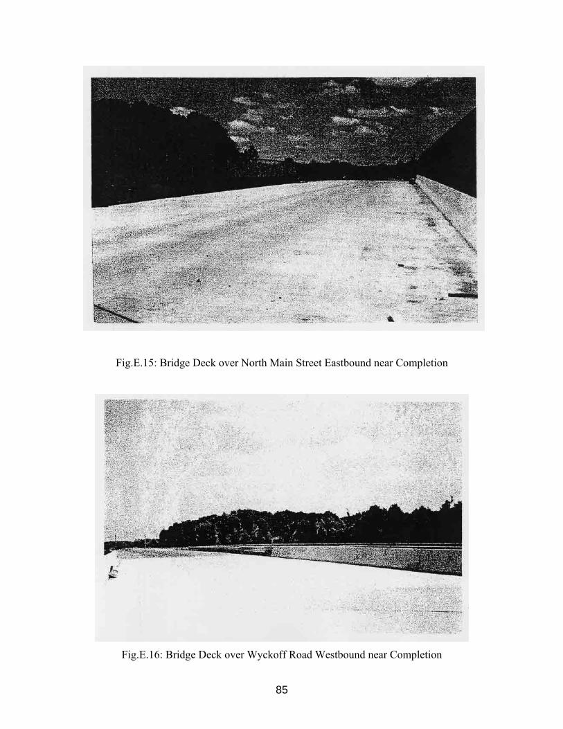
85
Fig.E.15: Bridge Deck over North Main Street Eastbound near Completion
Fig.E.16: Bridge Deck over Wyckoff Road Westbound near Completion

86
Fig.E.17: Bridge Deck over Wyckoff Road Eastbound near Completion
Fig.E.18: Bridge Deck over Rout 130 Westbound near Completion
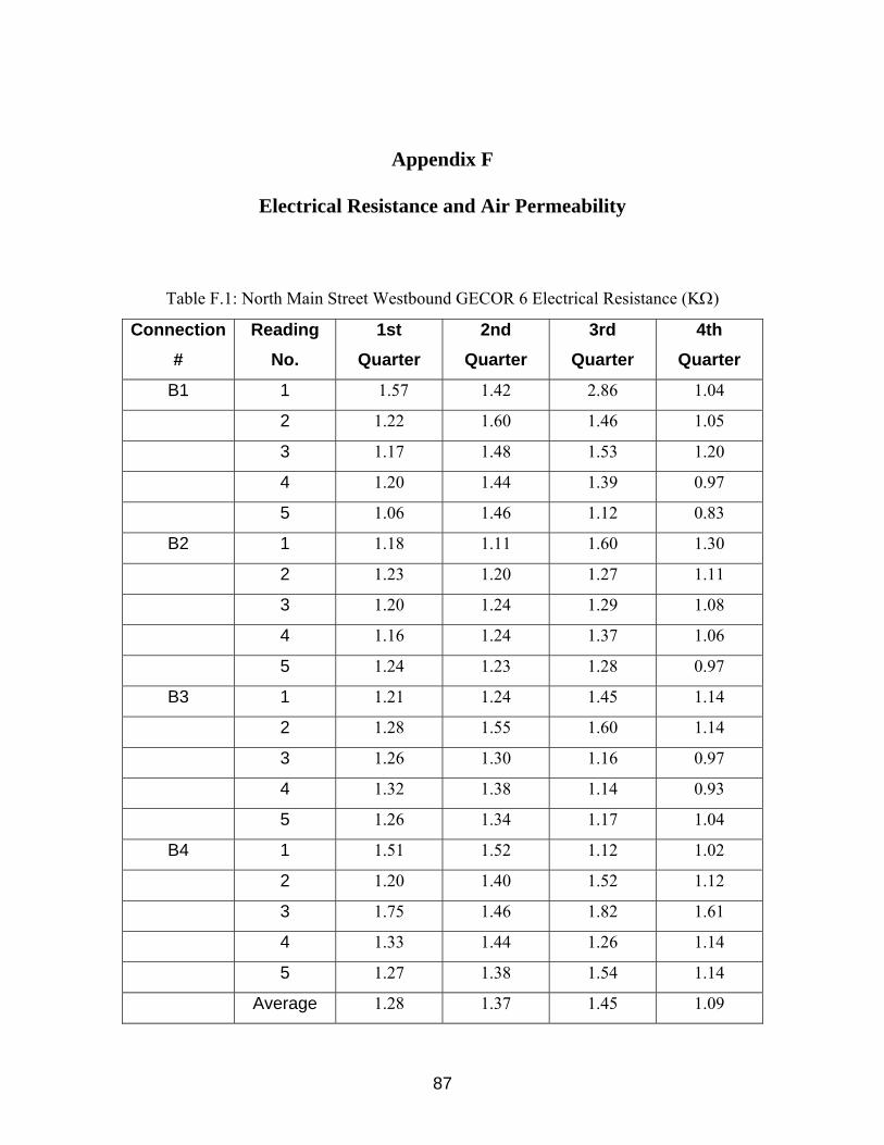
87
Appendix F
Electrical Resistance and Air Permeability
Table F.1: North Main Street Westbound GECOR 6 Electrical Resistance (KΩ)
Connection #
Reading No.
1st Quarter
2nd Quarter
3rd Quarter
4th Quarter
B1 1 1.57 1.42 2.86 1.04
2 1.22 1.60 1.46 1.05
3 1.17 1.48 1.53 1.20
4 1.20 1.44 1.39 0.97
5 1.06 1.46 1.12 0.83
B2 1 1.18 1.11 1.60 1.30
2 1.23 1.20 1.27 1.11
3 1.20 1.24 1.29 1.08
4 1.16 1.24 1.37 1.06
5 1.24 1.23 1.28 0.97
B3 1 1.21 1.24 1.45 1.14
2 1.28 1.55 1.60 1.14
3 1.26 1.30 1.16 0.97
4 1.32 1.38 1.14 0.93
5 1.26 1.34 1.17 1.04
B4 1 1.51 1.52 1.12 1.02
2 1.20 1.40 1.52 1.12
3 1.75 1.46 1.82 1.61
4 1.33 1.44 1.26 1.14
5 1.27 1.38 1.54 1.14
Average 1.28 1.37 1.45 1.09

88
Table F.2: North Main Street Westbound Air Permeability Vacuum (mm Hg), SCCM
(ml/min)
Table F.3: North Main Street Westbound Electrical Resistance Sealer Test (kΩ)
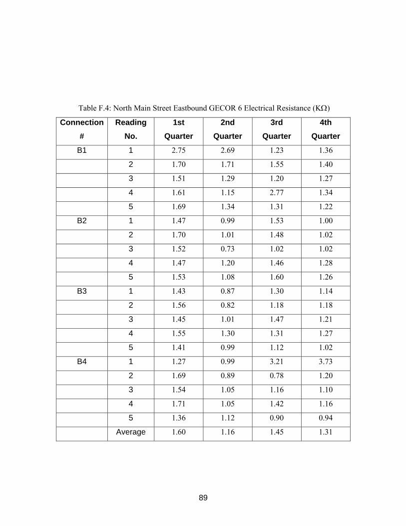
89
Table F.4: North Main Street Eastbound GECOR 6 Electrical Resistance (KΩ)
Connection #
Reading No.
1st Quarter
2nd Quarter
3rd Quarter
4th Quarter
B1 1 2.75 2.69 1.23 1.36
2 1.70 1.71 1.55 1.40
3 1.51 1.29 1.20 1.27
4 1.61 1.15 2.77 1.34
5 1.69 1.34 1.31 1.22
B2 1 1.47 0.99 1.53 1.00
2 1.70 1.01 1.48 1.02
3 1.52 0.73 1.02 1.02
4 1.47 1.20 1.46 1.28
5 1.53 1.08 1.60 1.26
B3 1 1.43 0.87 1.30 1.14
2 1.56 0.82 1.18 1.18
3 1.45 1.01 1.47 1.21
4 1.55 1.30 1.31 1.27
5 1.41 0.99 1.12 1.02
B4 1 1.27 0.99 3.21 3.73
2 1.69 0.89 0.78 1.20
3 1.54 1.05 1.16 1.10
4 1.71 1.05 1.42 1.16
5 1.36 1.12 0.90 0.94
Average 1.60 1.16 1.45 1.31

90
Table F.5: North Main Street Eastbound Air Permeability Vacuum (mm Hg), SCCM (ml/min)
Table F.6: North Main Street Eastbound Electrical Resistance Sealer Test (KΩ)

91
Table F.7: Wyckoff Road Westbound GECOR 6 Electrical Resistance (KΩ)
Connection #
Reading No.
1st Quarter
2nd Quarter
3rd Quarter
4th Quarter
B1 1 4.47 1.96 3.43 2.05
2 4.83 1.57 3.02 2.46
3 3.43 1.11 2.98 1.44
4 2.47 2.21 2.87 1.63
5 3.00 1.58 3.07 1.19
B2 1 3.77 1.45 3.22 1.34
2 3.67 1.32 2.53 1.37
3 2.90 1.24 2.91 1.06
4 2.80 1.15 2.22 1.22
5 2.54 1.30 3.30 1.13
B3 1 2.67 1.36 1.54 1.37
2 2.72 1.49 2.64 1.34
3 3.25 1.40 1.93 1.25
4 2.28 1.09 2.51 1.20
5 2.72 1.46 3.23 0.89
B4 1 3.20 1.86 4.15 0.98
2 2.99 1.56 2.92 0.96
3 3.33 1.86 2.52 0.97
4 3.05 1.75 2.42 0.99
5 2.89 1.87 2.66 0.87
Average 3.15 1.53 2.80 1.29

92
Table F.8: Wyckoff Road Westbound Air Permeability Vacuum (mm Hg), SCCM (ml/min)
Table F.9: Wyckoff Road Westbound Electrical Resistance Sealer Test (KΩ)

93
Table F.10: Wyckoff Road Eastbound GECOR 6 Electrical Resistance (KΩ)
Connection #
Reading No.
1st Quarter
2nd Quarter
3rd Quarter
4th Quarter
B1 1 3.54 1.72 2.09 1.89
2 4.17 1.91 1.55 2.31
3 3.14 1.72 1.44 2.36
4 1.20 1.11 1.45 2.05
5 1.75 0.85 1.37 2.11
B2 1 1.67 0.72 1.42 2.05
2 2.04 0.73 1.45 2.04
3 1.59 1.01 1.40 2.18
4 1.72 1.11 1.38 1.55
5 1.74 1.07 1.46 2.16
B3 1 1.84 0.87 1.61 1.45
2 1.48 0.95 1.70 1.83
3 1.60 0.69 1.62 1.28
4 1.94 0.71 1.65 1.89
5 1.83 0.85 1.34 2.37
B4 1 5.16 1.16 1.32 1.81
2 3.97 0.90 1.48 2.02
3 2.05 0.73 0.97 2.22
4 2.02 1.03 1.53 1.85
5 1.67 0.85 1.46 2.20
Average 2.31 1.05 1.48 1.99
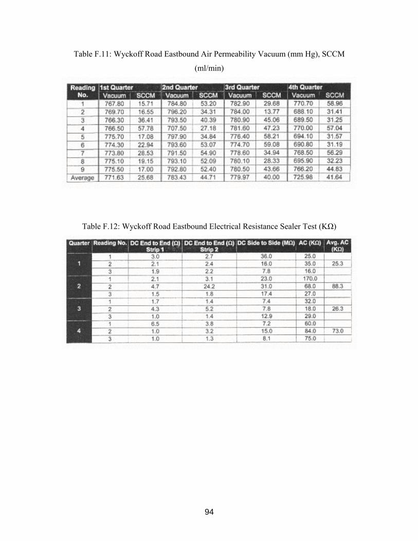
94
Table F.11: Wyckoff Road Eastbound Air Permeability Vacuum (mm Hg), SCCM
(ml/min)
Table F.12: Wyckoff Road Eastbound Electrical Resistance Sealer Test (KΩ)
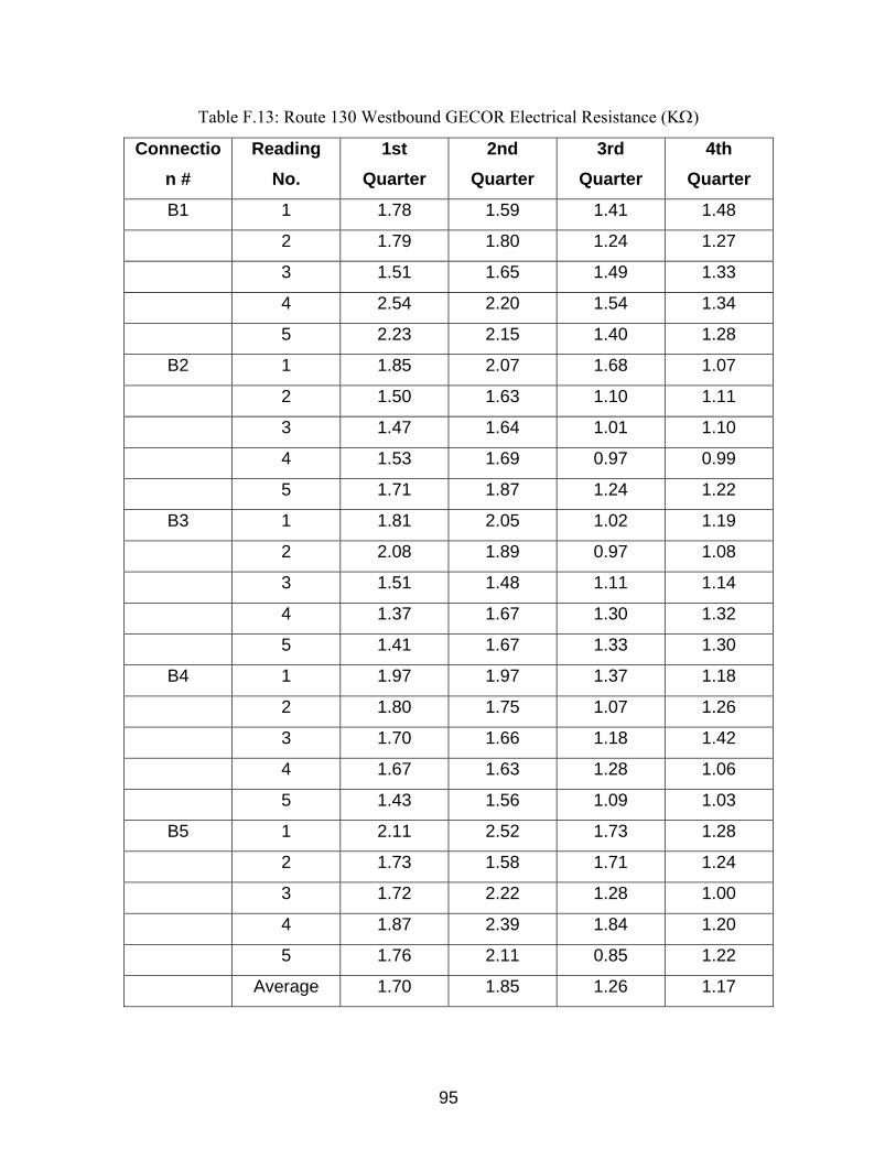
95
Table F.13: Route 130 Westbound GECOR Electrical Resistance (KΩ)
Connection #
Reading No.
1st Quarter
2nd Quarter
3rd Quarter
4th Quarter
B1 1 1.78 1.59 1.41 1.48
2 1.79 1.80 1.24 1.27
3 1.51 1.65 1.49 1.33
4 2.54 2.20 1.54 1.34
5 2.23 2.15 1.40 1.28
B2 1 1.85 2.07 1.68 1.07
2 1.50 1.63 1.10 1.11
3 1.47 1.64 1.01 1.10
4 1.53 1.69 0.97 0.99
5 1.71 1.87 1.24 1.22
B3 1 1.81 2.05 1.02 1.19
2 2.08 1.89 0.97 1.08
3 1.51 1.48 1.11 1.14
4 1.37 1.67 1.30 1.32
5 1.41 1.67 1.33 1.30
B4 1 1.97 1.97 1.37 1.18
2 1.80 1.75 1.07 1.26
3 1.70 1.66 1.18 1.42
4 1.67 1.63 1.28 1.06
5 1.43 1.56 1.09 1.03
B5 1 2.11 2.52 1.73 1.28
2 1.73 1.58 1.71 1.24
3 1.72 2.22 1.28 1.00
4 1.87 2.39 1.84 1.20
5 1.76 2.11 0.85 1.22
Average 1.70 1.85 1.26 1.17
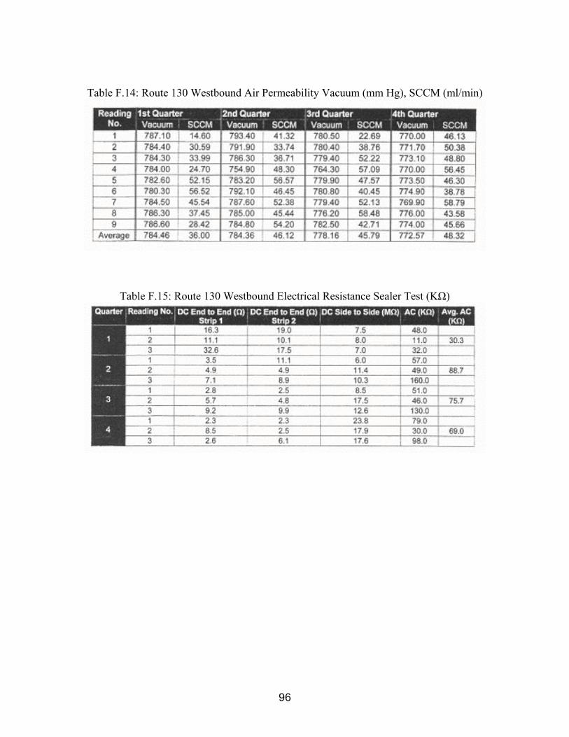
96
Table F.14: Route 130 Westbound Air Permeability Vacuum (mm Hg), SCCM (ml/min)
Table F.15: Route 130 Westbound Electrical Resistance Sealer Test (KΩ)

97
Appendix G
Corrosion Measurements

98
Table G.1: Minideck A – ASTM G 109 Corrosion Rate (µA/cm2)
Specimen Cycle 1
Cycle 2
Cycle 3
Cycle 4
Cycle 5
Cycle 6
Cycle 7
Cycle 8
Cycle 9
Cycle 10
Cycle 11
A1 0.60 0.90 0.60 0.90 1.00 0.90 0.90 1.00 0.15 0.08 0.18 A2 0.30 0.60 0.70 0.80 1.00 0.80 1.00 0.90 0.18 0.08 0.25 A3 0.20 1.00 0.60 1.10 1.00 1.10 1.50 1.50 0.73 0.73 0.90
A4 1.00 0.50 0.30 0.70 0.80 0.70 0.80 0.80 0.03 0.08 0.08
A5 0.30 0.10 0.10 0.00 0.40 0.10 0.10 0.20 0.03 0.15 0.03
A6 0.10 0.30 0.30 0.50 0.40 0.30 0.40 0.40 0.10 0.15 0.15
Average 0.42 0.57 0.43 0.67 0.77 0.65 0.78 0.80 0.20 0.21 0.26
Specimen Cycle
12 Cycle
13 Cycle
14 Cycle
15 Cycle
16 Cycle
17 Cycle
18 Cycle
19 Cycle
20 Cycle
21 Cycle
22
A1 0.03 0.11 0.09 0.59 0.20 0.40 10.10 1.10 12.80 7.50 9.60
A2 0.04 0.14 0.13 0.00 0.30 0.04 0.00 0.30 7.80 2.30 2.00
A3 0.04 0.60 0.57 0.00 0.30 0.03 1.60 0.70 1.00 2.20 4.60
A4 0.08 0.06 0.07 0.17 0.80 0.98 0.30 0.10 0.10 0.10 0.20
A5 0.00 0.05 0.06 0.00 3.40 3.80 0.50 0.27 8.20 1.40 2.30
A6 0.01 0.10 0.10 0.07 0.10 0.20 0.40 0.30 0.10 0.10 0.20
Average 0.03 0.18 0.17 0.14 0.85 0.91 2.15 0.46 5.00 2.27 3.15

99
Table G.2: Minideck A – ASTM G 109 Corrosion Potential (mV)
Specimen Cycle 1
Cycle 2
Cycle 3
Cycle 4
Cycle 5
Cycle 6
Cycle 7
Cycle 8
Cycle 9
Cycle 10
Cycle 11
A1 N/A N/A -11.67 -12.12 -15.29 -13.88 -23.07 -12.54 -14.00 -6.92 -6.46 A2 N/A N/A -2.19 -1.48 -4.97 -3.06 -11.80 -1.09 0.01 -0.24 -0.15
A3 N/A N/A -0.75 -6.80 -5.39 -3.27 -10.46 -0.86 -23.51 -17.07 -14.38
A4 N/A N/A -2.07 -2.68 -7.36 -6.44 -16.03 -6.16 -15.69 -9.92 -7.67
A5 N/A N/A -5.60 -5.92 -10.28 -9.53 -18.69 -8.99 -23.76 -18.28 -15.48
A6 N/A N/A -13.58 -13.91 -18.46 -17.71 -27.64 -20.50 -33.82 -27.73 -25.14
Average N/A N/A -5.98 -7.15 -10.29 -8.98 -17.95 -8.36 -18.46 -13.36 -11.54
Specimen Cycle
12 Cycle
13 Cycle
14 Cycle
15 Cycle
16 Cycle
17 Cycle
18 Cycle
19 Cycle
20 Cycle
21 Cycle
22
A1 -4.81 -10.06 -4.90 -5.90 0.03 12.30 -259.7 111.45 2.72 21.39 2.58
A2 -0.12 -0.01 0.00 0.01 3.75 4.60 25.50 -6.25 1.23 9.20 1.24
A3 -11.22 -17.74 -11.64 -12.24 7.86 8.36 14.98 4.65 1.81 35.40 1.17
A4 -5.70 -10.91 -5.30 -4.51 13.30 13.65 20.00 0.98 1.94 4.90 0.89
A5 -13.43 -18.29 -12.53 -12.16 12.84 15.36 66.47 0.81 6.30 13.11 0.87
A6 -22.75 -28.77 -21.80 -21.53 4.01 5.01 -8.70 0.82 8.10 4.51 0.88
Average -9.67 -14.29 -9.36 -9.39 6.97 9.88 -23.58 18.74 3.68 14.75 1.27

100
-30.00
-25.00
-20.00
-15.00
-10.00
-5.00
0.00
5.00
10.00
15.00
20.00
25.00
0 1 2 3 4 5 6 7 8 9 10 11 12 13 14 15 16 17 18 19 20 21 22 23
Cycles
Cor
rosi
on P
oten
tial (
mV)
Fig G.1: Minideck A – Average Corrosion Potential (mV)
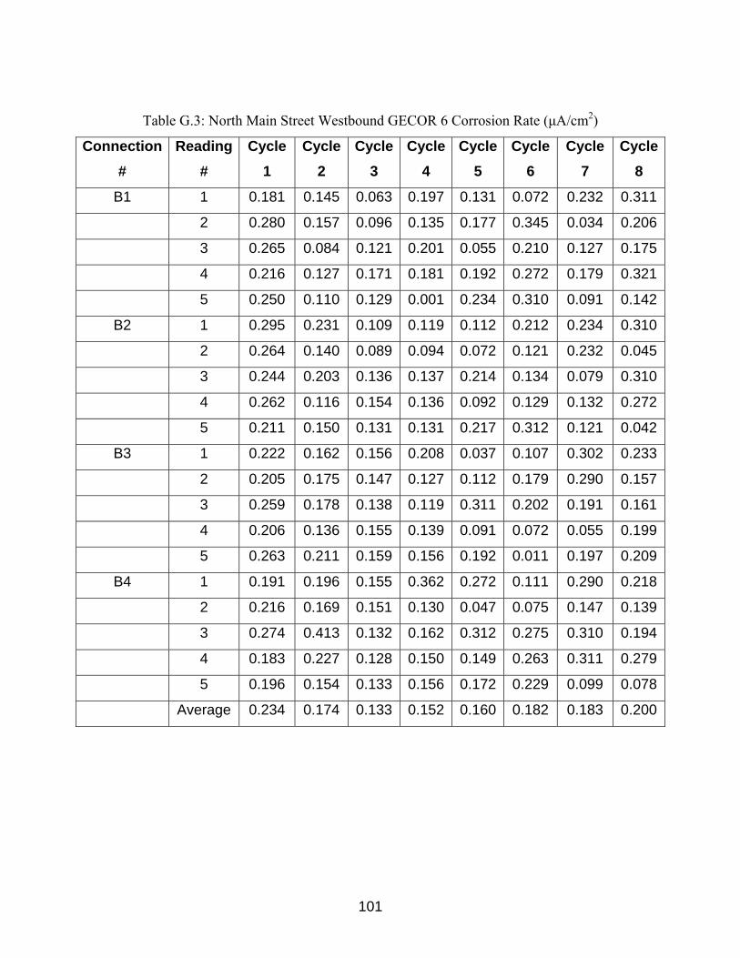
101
Table G.3: North Main Street Westbound GECOR 6 Corrosion Rate (µA/cm2)
Connection #
Reading #
Cycle 1
Cycle 2
Cycle 3
Cycle 4
Cycle 5
Cycle 6
Cycle 7
Cycle 8
B1 1 0.181 0.145 0.063 0.197 0.131 0.072 0.232 0.311
2 0.280 0.157 0.096 0.135 0.177 0.345 0.034 0.206
3 0.265 0.084 0.121 0.201 0.055 0.210 0.127 0.175
4 0.216 0.127 0.171 0.181 0.192 0.272 0.179 0.321
5 0.250 0.110 0.129 0.001 0.234 0.310 0.091 0.142
B2 1 0.295 0.231 0.109 0.119 0.112 0.212 0.234 0.310
2 0.264 0.140 0.089 0.094 0.072 0.121 0.232 0.045
3 0.244 0.203 0.136 0.137 0.214 0.134 0.079 0.310
4 0.262 0.116 0.154 0.136 0.092 0.129 0.132 0.272
5 0.211 0.150 0.131 0.131 0.217 0.312 0.121 0.042
B3 1 0.222 0.162 0.156 0.208 0.037 0.107 0.302 0.233
2 0.205 0.175 0.147 0.127 0.112 0.179 0.290 0.157
3 0.259 0.178 0.138 0.119 0.311 0.202 0.191 0.161
4 0.206 0.136 0.155 0.139 0.091 0.072 0.055 0.199
5 0.263 0.211 0.159 0.156 0.192 0.011 0.197 0.209
B4 1 0.191 0.196 0.155 0.362 0.272 0.111 0.290 0.218
2 0.216 0.169 0.151 0.130 0.047 0.075 0.147 0.139
3 0.274 0.413 0.132 0.162 0.312 0.275 0.310 0.194
4 0.183 0.227 0.128 0.150 0.149 0.263 0.311 0.279
5 0.196 0.154 0.133 0.156 0.172 0.229 0.099 0.078
Average 0.234 0.174 0.133 0.152 0.160 0.182 0.183 0.200

102
Table G.4: Main Street Westbound GECOR 6 Corrosion Potential (mV)
Connection #
Reading #
Cycle 1
Cycle 2
Cycle 3
Cycle 4
Cycle 5
Cycle 6
Cycle 7
Cycle 8
B1 1 -88.8 -127.4 -220.7 -234.9 -249.1 -252.3 -190.4 -170.9
2 -56.2 -128.1 -168.6 -154.2 -94.4 -197.1 -270.3 -141.2
3 -63.5 -124.5 -190.3 -202.5 -97.2 -242.4 -179.1 -157.6
4 -75.9 -140.9 -183.2 -194.3 -170.2 -73.2 -84.6 -121.4
5 -83.0 -133.4 -187.8 -192.7 -201.9 -214.3 -197.2 -212.4
B2 1 -78.2 -126.4 -214.7 -219.7 -181.1 -99.3 -147.4 -212.4
2 -84.1 -87.8 -211.8 -218.7 -178.6 -109.5 -88.2 -153.2
3 -73.5 -123.6 -218.8 -227.1 -91.7 -205.4 -167.6 -221.3
4 -76.4 -120.8 -227.5 -233.2 -192.4 -146.0 -81.7 -159.3
5 -73.6 -126.3 -221.1 -235.8 -78.7 -200.3 -100.4 -166.6
B3 1 -86.4 -108.6 -233.3 -253.5 -89.4 -104.6 -111.8 -191.4
2 -95.5 -116.7 -240.4 -249.7 -107.5 -92.4 -207.9 -129.3
3 -99.8 -116.1 -266.2 -267.4 -192.4 -187.4 -201.2 -148.5
4 -89.9 -126.5 -213.3 -220.5 -148.5 -84.9 -97.3 -94.7
5 -95.7 -142.3 -216.6 -226.3 -204.4 -79.8 -87.2 -148.5
B4 1 -91.2 -142.9 -203.3 -239.2 -141.4 -114.3 -186.7 -202.4
2 -98.5 -131.5 -222.4 -245.3 -187.2 -172.5 -155.5 -191.6
3 -83.1 -153.3 -203.8 -227.6 -121.4 -76.4 -89.2 -104.8
4 -83.2 -141.5 -169.7 -181.7 -200.4 -22.3 -270.5 -91.0
5 -91.7 -142.3 -191.1 -201.9 -158.5 -167.5 -176.5 -214.9
Average -83.4 -128.0 -210.2 -221.3 -154.3 -142.1 -154.5 -219.6

103
-250
-200
-150
-100
-50
0Cycle 1 Cycle 2 Cycle 3 Cycle 4 Cycle 5 Cycle 6 Cycle 7 Cycle 8
Cy c l e s
Fig G.2: North Main Street Westbound GECOR 6 Average Corrosion Potential
(mV)
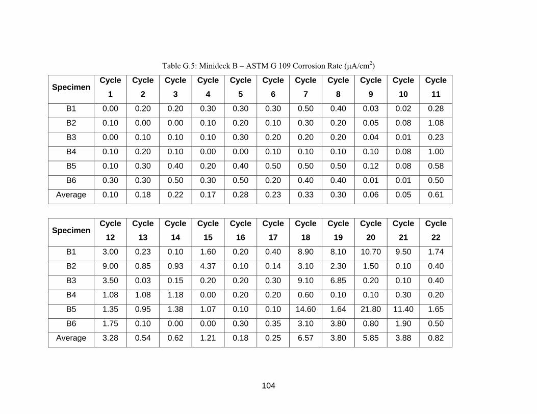
104
Table G.5: Minideck B – ASTM G 109 Corrosion Rate (µA/cm2)
Specimen Cycle
1 Cycle
2 Cycle
3 Cycle
4 Cycle
5 Cycle
6 Cycle
7 Cycle
8 Cycle
9 Cycle
10 Cycle
11
B1 0.00 0.20 0.20 0.30 0.30 0.30 0.50 0.40 0.03 0.02 0.28
B2 0.10 0.00 0.00 0.10 0.20 0.10 0.30 0.20 0.05 0.08 1.08
B3 0.00 0.10 0.10 0.10 0.30 0.20 0.20 0.20 0.04 0.01 0.23
B4 0.10 0.20 0.10 0.00 0.00 0.10 0.10 0.10 0.10 0.08 1.00
B5 0.10 0.30 0.40 0.20 0.40 0.50 0.50 0.50 0.12 0.08 0.58
B6 0.30 0.30 0.50 0.30 0.50 0.20 0.40 0.40 0.01 0.01 0.50
Average 0.10 0.18 0.22 0.17 0.28 0.23 0.33 0.30 0.06 0.05 0.61
Specimen Cycle
12 Cycle
13 Cycle
14 Cycle
15 Cycle
16 Cycle
17 Cycle
18 Cycle
19 Cycle
20 Cycle
21 Cycle
22
B1 3.00 0.23 0.10 1.60 0.20 0.40 8.90 8.10 10.70 9.50 1.74
B2 9.00 0.85 0.93 4.37 0.10 0.14 3.10 2.30 1.50 0.10 0.40
B3 3.50 0.03 0.15 0.20 0.20 0.30 9.10 6.85 0.20 0.10 0.40
B4 1.08 1.08 1.18 0.00 0.20 0.20 0.60 0.10 0.10 0.30 0.20
B5 1.35 0.95 1.38 1.07 0.10 0.10 14.60 1.64 21.80 11.40 1.65
B6 1.75 0.10 0.00 0.00 0.30 0.35 3.10 3.80 0.80 1.90 0.50
Average 3.28 0.54 0.62 1.21 0.18 0.25 6.57 3.80 5.85 3.88 0.82

105
Table G.6: Minideck B – ASTM G 109 Corrosion Potential (mV)
Specimen Cycle
1 Cycle
2 Cycle 3
Cycle 4
Cycle 5
Cycle 6
Cycle 7
Cycle 8
Cycle 9
Cycle 10
Cycle 11
B1 N/A N/A -21.52 -21.55 -24.51 -21.98 -31.16 -20.19 -26.17 -20.37 -17.64
B2 N/A N/A -18.61 -17.65 -20.35 -18.32 -27.87 -15.69 -22.09 -16.20 -13.09
B3 N/A N/A -20.51 -23.42 -30.03 -31.47 -45.88 -37.66 -79.59 -46.00 -42.09
B4 N/A N/A -19.45 -19.27 -21.94 -19.32 -28.53 -17.60 -38.37 -31.75 -29.60
B5 N/A N/A -17.75 -17.26 -20.33 -17.48 -25.77 -14.35 -22.72 -17.36 -15.29
B6 N/A N/A -6033 -18.64 -22.87 -23.64 -35.04 -27.19 -11.72 -5.68 -2.41
Average N/A N/A -19.03 -19.63 -23.34 -22.04 -32.38 -22.11 -33.44 -22.89 -20.02
Specimen Cycle
12 Cycle
13 Cycle
14 Cycle
15 Cycle
16 Cycle
17 Cycle
18 Cycle
19 Cycle
20 Cycle
21 Cycle
22
B1 -15.98 -20.55 -16.22 -16.55 8.88 9.32 288.94 74.22 8.32 16.55 1.05
B2 -11.38 -17.32 -11.41 -11.15 16.37 16.39 3.50 2.52 7.05 3.96 0.93
B3 -42.84 -62.92 -40.95 -41.25 18.45 20.15 12.58 6.19 10.18 4.60 1.45
B4 -29.39 -33.95 -29.19 -28.82 9.16 10.23 7.45 5.15 3.26 2.95 1.60
B5 -6.87 -18.99 -13.32 -13.14 17.98 19.56 262.68 4.57 5.68 10.99 1.95
B6 -0.67 -6.12 -0.39 -0.43 18.05 20.58 8.78 5.95 4.04 3.18 2.55
Average -17.85 -26.64 -18.58 -18.55 14.82 16.04 97.32 16.43 6.42 7.04 1.59

106
-40.00
-20.00
0.00
20.00
40.00
60.00
80.00
100.00
120.00
0 1 2 3 4 5 6 7 8 9 10 11 12 13 14 15 16 17 18 19 20 21 22 23
Cycles
Cor
rosi
on P
oten
tial (
mV)
Fig. G.3: Minideck B – Average Corrosion Potential (mV)
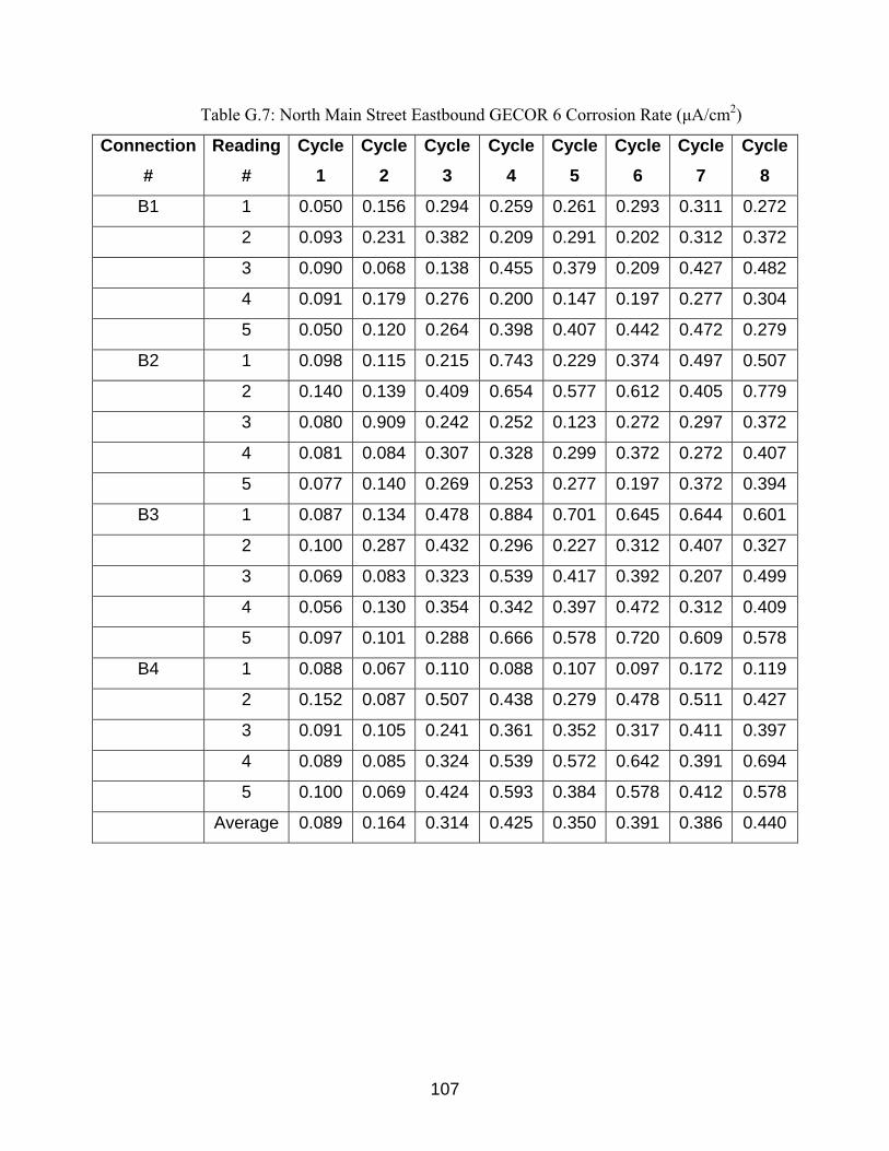
107
Table G.7: North Main Street Eastbound GECOR 6 Corrosion Rate (µA/cm2)
Connection #
Reading #
Cycle 1
Cycle 2
Cycle 3
Cycle 4
Cycle 5
Cycle 6
Cycle 7
Cycle 8
B1 1 0.050 0.156 0.294 0.259 0.261 0.293 0.311 0.272
2 0.093 0.231 0.382 0.209 0.291 0.202 0.312 0.372
3 0.090 0.068 0.138 0.455 0.379 0.209 0.427 0.482
4 0.091 0.179 0.276 0.200 0.147 0.197 0.277 0.304
5 0.050 0.120 0.264 0.398 0.407 0.442 0.472 0.279
B2 1 0.098 0.115 0.215 0.743 0.229 0.374 0.497 0.507
2 0.140 0.139 0.409 0.654 0.577 0.612 0.405 0.779
3 0.080 0.909 0.242 0.252 0.123 0.272 0.297 0.372
4 0.081 0.084 0.307 0.328 0.299 0.372 0.272 0.407
5 0.077 0.140 0.269 0.253 0.277 0.197 0.372 0.394
B3 1 0.087 0.134 0.478 0.884 0.701 0.645 0.644 0.601
2 0.100 0.287 0.432 0.296 0.227 0.312 0.407 0.327
3 0.069 0.083 0.323 0.539 0.417 0.392 0.207 0.499
4 0.056 0.130 0.354 0.342 0.397 0.472 0.312 0.409
5 0.097 0.101 0.288 0.666 0.578 0.720 0.609 0.578
B4 1 0.088 0.067 0.110 0.088 0.107 0.097 0.172 0.119
2 0.152 0.087 0.507 0.438 0.279 0.478 0.511 0.427
3 0.091 0.105 0.241 0.361 0.352 0.317 0.411 0.397
4 0.089 0.085 0.324 0.539 0.572 0.642 0.391 0.694
5 0.100 0.069 0.424 0.593 0.384 0.578 0.412 0.578
Average 0.089 0.164 0.314 0.425 0.350 0.391 0.386 0.440
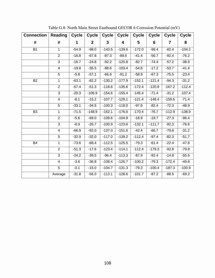
108
Table G.8: North Main Street Eastbound GECOR 6 Corrosion Potential (mV)
Connection #
Reading #
Cycle 1
Cycle 2
Cycle 3
Cycle 4
Cycle 5
Cycle 6
Cycle 7
Cycle 8
B1 1 -54.9 -98.0 -143.5 -139.6 -172.0 -98.4 -82.4 -104.2
2 -16.8 -67.8 -87.3 -89.6 -41.4 -56.7 -92.4 -76.2
3 -16.7 -24.8 -92.2 -125.8 -82.7 -74.4 -57.2 -38.9
4 -19.8 -35.5 -88.6 -103.4 -54.8 -17.2 -53.7 -41.4
5 -5.8 -57.1 -66.6 -91.2 -58.9 -67.3 -75.5 -23.4
B2 1 -63.1 -82.2 -130.2 -177.9 -152.1 -121.4 -94.3 -31.2
2 -57.4 -51.3 -118.6 -135.6 -172.4 -120.9 -167.2 -112.4
3 -20.3 -106.9 -154.6 -155.4 -145.4 -71.4 -31.2 -107.4
4 -8.1 -15.2 -107.7 -129.1 -121.4 -148.4 -159.6 -71.4
5 -33.1 -34.5 -100.3 -118.0 -97.6 -82.4 -72.3 -48.9
B3 1 -71.5 -148.9 -162.1 -176.6 -170.4 -76.7 -112.9 -138.9
2 -5.6 -69.0 -109.6 -104.9 -18.9 -19.7 -27.3 -96.4
3 -6.9 -26.7 -100.9 -123.6 -132.1 -111.7 -92.3 -76.6
4 -66.9 -92.0 -137.0 -151.6 -42.4 -66.7 -79.8 -31.2
5 -32.9 -32.0 -117.0 -139.2 -112.4 -97.4 -82.3 -51.7
B4 1 -73.6 -68.4 -112.5 -125.5 -79.3 -61.4 -22.4 -47.8
2 -51.3 -17.6 -123.4 -114.1 -112.4 -179.3 -92.8 -79.8
3 -24.2 -39.5 -96.4 -113.3 -87.9 -92.4 -14.8 -55.6
4 -3.6 -36.8 -108.4 -126.7 -100.2 -79.3 -172.4 -49.8
5 -3.1 -15.0 -104.7 -131.3 -79.3 -100.4 -187.3 -100.9
Average -31.8 -56.0 -113.1 -128.6 -101.7 -87.2 -88.5 -69.2

109
-230.0
-180.0
-130.0
-80.0
-30.0
Cycle 1 Cycle 2 Cycle 3 Cycle 4 Cycle 5 Cycle 6 Cycle 7 Cycle 8Cy c l e s
Fig. G.4: North Main Street Eastbound GEOCOR 6 Average Corrosion Potential
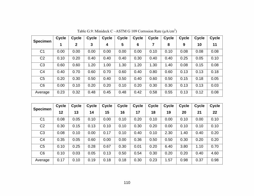
110
Table G.9: Minideck C –ASTM G 109 Corrosion Rate (µA/cm2)
Specimen Cycle
1 Cycle
2 Cycle
3 Cycle
4 Cycle
5 Cycle
6 Cycle
7 Cycle
8 Cycle
9 Cycle
10 Cycle
11
C1 0.00 0.00 0.00 0.00 0.00 0.00 0.10 0.10 0.08 0.08 0.08
C2 0.10 0.20 0.40 0.40 0.40 0.30 0.40 0.40 0.25 0.05 0.10
C3 0.60 0.60 1.20 1.00 1.30 1.20 1.30 1.40 0.08 0.15 0.08
C4 0.40 0.70 0.60 0.70 0.60 0.40 0.80 0.60 0.13 0.13 0.18
C5 0.20 0.30 0.50 0.40 0.50 0.40 0.60 0.50 0.15 0.18 0.05
C6 0.00 0.10 0.20 0.20 0.10 0.20 0.30 0.30 0.13 0.13 0.03
Average 0.23 0.32 0.48 0.45 0.48 0.42 0.58 0.55 0.13 0.12 0.08
Specimen Cycle
12 Cycle
13 Cycle
14 Cycle
15 Cycle
16 Cycle
17 Cycle
18 Cycle
19 Cycle
20 Cycle
21 Cycle
22
C1 0.08 0.05 0.10 0.00 0.10 0.20 0.10 0.00 0.10 0.00 0.10
C2 0.30 0.15 0.13 0.10 0.10 0.30 0.20 0.00 0.10 0.10 0.10
C3 0.08 0.10 0.00 0.17 0.10 0.40 0.10 2.30 1.40 0.40 0.20
C4 0.35 0.05 0.60 0.00 0.00 0.36 0.50 0.50 0.30 0.20 0.20
C5 0.10 0.25 0.28 0.67 0.30 0.01 0.20 6.40 3.80 1.10 0.70
C6 0.10 0.03 0.05 0.13 0.50 0.54 0.30 0.20 0.20 0.40 4.60
Average 0.17 0.10 0.19 0.18 0.18 0.30 0.23 1.57 0.98 0.37 0.98

111
Table G.10: Minideck C – ASTM G 109 Corrosion Potential (mV)
Specimen Cycle
1 Cycle
2 Cycle
3 Cycle
4 Cycle
5 Cycle
6 Cycle
7 Cycle
8 Cycle
9 Cycle
10 Cycle
11
C1 N/A N/A -14.31 -13.82 -17.82 -14.80 -25.45 -12.50 -20.66 -13.29 -9.80
C2 N/A N/A -6.39 -6.22 -10.01 -6.85 -17.94 -7.23 -28.25 -20.42 -17.09
C3 N/A N/A -32.81 -31.44 -36.36 -33.52 -44.23 -30.50 -44.44 -35.74 -32.29
C4 N/A N/A -35.54 -34.81 -38.87 -35.27 -46.52 -33.90 -25.49 -17.90 -14.56
C5 N/A N/A -14.24 -13.47 -18.28 -16.65 -27.81 -16.43 -37.27 -29.33 -25.47
C6 N/A N/A -21.82 -21.75 -25.78 -23.66 -35.38 -23.36 1.01 12.72 16.38
Average N/A N/A -20.85 -20.25 -24.52 -21.79 -32.89 -20.65 -25.85 -17.33 -13.80
Specimen Cycle
12 Cycle
13 Cycle
14 Cycle
15 Cycle
16 Cycle
17 Cycle
18 Cycle
19 Cycle
20 Cycle
21 Cycle
22
C1 -7.66 -15.28 -8.76 -9.09 17.42 18.02 11.52 11.52 5.66 2.02 3.56
C2 -15.19 -23.37 -15.52 -12.15 17.72 18.36 20.15 0.95 2.98 3.54 1.48
C3 -29.96 -39.37 -30.18 -22.11 17.66 20.25 3.58 0.96 5.44 10.55 1.40
C4 -12.53 -20.60 -12.33 -20.98 3.53 4.00 -2.25 15.39 3.09 2.06 2.66
C5 -23.60 -32.43 -22.48 -29.12 3.26 4.36 15.43 263.60 3.99 179.64 1.05
C6 18.86 7.64 20.99 12.00 16.25 19.36 12.42 -1.37 4.10 51.40 0.95
Average -11.68 -20.57 -11.38 -13.57 12.64 14.06 10.14 48.51 4.21 41.54 1.85
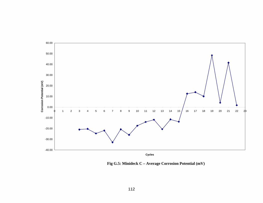
112
-40.00
-30.00
-20.00
-10.00
0.00
10.00
20.00
30.00
40.00
50.00
60.00
0 1 2 3 4 5 6 7 8 9 10 11 12 13 14 15 16 17 18 19 20 21 22 23
Cycles
Cor
rosi
on P
oten
tial (
mV)
Fig G.5: Minideck C – Average Corrosion Potential (mV)

113
Table G.11: Wyckoff Road Westbound GECOR 6 Corrosion Rate (µA/cm2)
Connection #
Reading #
Cycle 1
Cycle 2
Cycle 3
Cycle 4
Cycle 5
Cycle 6
Cycle 7
Cycle 8
B1 1 0.061 0.150 0.069 0.381 0.217 0.229 0.394 0.462
2 0.040 0.095 0.057 0.315 0.085 0.197 0.402 0.472
3 0.063 0.098 0.066 0.434 0.279 0.127 0.397 0.272
4 0.082 0.155 0.065 0.119 0.372 0.402 0.287 0.197
5 0.064 0.110 0.031 0.567 0.599 0.379 0.234 0.099
B2 1 0.069 0.188 0.037 0.233 0.112 0.087 0.217 0.307
2 0.059 0.114 0.049 0.233 0.297 0.187 0.398 0.402
3 0.083 0.104 0.044 0.336 0.205 0.112 0.077 0.325
4 0.067 0.144 0.046 0.312 0.372 0.424 0.278 0.221
5 0.089 0.176 0.059 0.558 0.599 0.473 0.372 0.617
B3 1 0.100 0.121 0.276 0.223 0.227 0.079 0.114 0.472
2 0.116 0.248 0.051 0.303 0.409 0.198 0.224 0.395
3 0.059 0.204 0.096 0.324 0.221 0.188 0.272 0.155
4 0.064 0.117 0.048 0.263 0.255 0.097 0.072 0.137
5 0.072 0.150 0.030 0.468 0.572 0.432 0.397 0.482
B4 1 0.075 0.181 0.021 0.492 0.572 0.302 0.272 0.599
2 0.126 0.209 0.032 0.441 0.277 0.124 0.343 0.407
3 0.068 0.079 0.043 0.277 0.317 0.297 0.397 0.317
4 0.107 0.191 0.044 0.309 0.402 0.198 0.272 0.612
5 0.066 0.136 0.042 0.347 0.192 0.355 0.473 0.578
Average 0.077 0.149 0.060 0.347 0.329 0.244 0.295 0.376
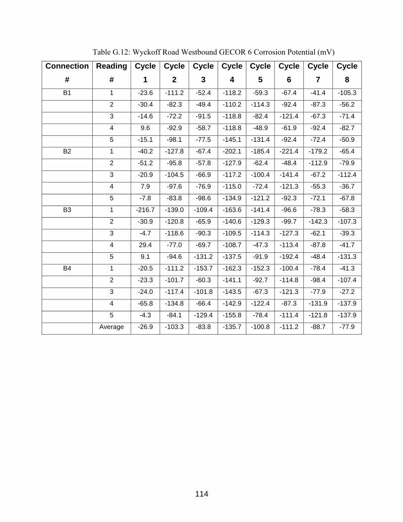
114
Table G.12: Wyckoff Road Westbound GECOR 6 Corrosion Potential (mV)
Connection #
Reading #
Cycle 1
Cycle 2
Cycle 3
Cycle 4
Cycle 5
Cycle 6
Cycle 7
Cycle 8
B1 1 -23.6 -111.2 -52.4 -118.2 -59.3 -67.4 -41.4 -105.3
2 -30.4 -82.3 -49.4 -110.2 -114.3 -92.4 -87.3 -56.2
3 -14.6 -72.2 -91.5 -118.8 -82.4 -121.4 -67.3 -71.4
4 9.6 -92.9 -58.7 -118.8 -48.9 -61.9 -92.4 -82.7
5 -15.1 -98.1 -77.5 -145.1 -131.4 -92.4 -72.4 -50.9
B2 1 -40.2 -127.8 -67.4 -202.1 -185.4 -221.4 -179.2 -65.4
2 -51.2 -95.8 -57.8 -127.9 -62.4 -48.4 -112.9 -79.9
3 -20.9 -104.5 -66.9 -117.2 -100.4 -141.4 -67.2 -112.4
4 7.9 -97.6 -76.9 -115.0 -72.4 -121.3 -55.3 -36.7
5 -7.8 -83.8 -98.6 -134.9 -121.2 -92.3 -72.1 -67.8
B3 1 -216.7 -139.0 -109.4 -163.6 -141.4 -96.6 -78.3 -58.3
2 -30.9 -120.8 -65.9 -140.6 -129.3 -99.7 -142.3 -107.3
3 -4.7 -118.6 -90.3 -109.5 -114.3 -127.3 -62.1 -39.3
4 29.4 -77.0 -69.7 -108.7 -47.3 -113.4 -87.8 -41.7
5 9.1 -94.6 -131.2 -137.5 -91.9 -192.4 -48.4 -131.3
B4 1 -20.5 -111.2 -153.7 -162.3 -152.3 -100.4 -78.4 -41.3
2 -23.3 -101.7 -60.3 -141.1 -92.7 -114.8 -98.4 -107.4
3 -24.0 -117.4 -101.8 -143.5 -67.3 -121.3 -77.9 -27.2
4 -65.8 -134.8 -66.4 -142.9 -122.4 -87.3 -131.9 -137.9
5 -4.3 -84.1 -129.4 -155.8 -78.4 -111.4 -121.8 -137.9
Average -26.9 -103.3 -83.8 -135.7 -100.8 -111.2 -88.7 -77.9
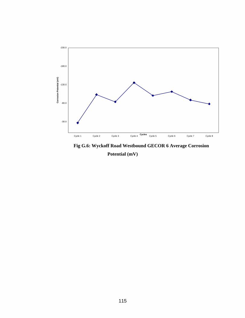
115
-230.0
-180.0
-130.0
-80.0
-30.0
Cycle 1 Cycle 2 Cycle 3 Cycle 4 Cycle 5 Cycle 6 Cycle 7 Cycle 8Cycles
Cor
rosi
on P
oten
tial (
mV)
Fig G.6: Wyckoff Road Westbound GECOR 6 Average Corrosion
Potential (mV)
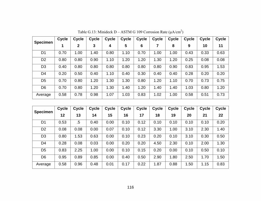
116
Table G.13: Minideck D – ASTM G 109 Corrosion Rate (µA/cm2)
Specimen Cycle
1 Cycle
2 Cycle
3 Cycle
4 Cycle
5 Cycle
6 Cycle
7 Cycle
8 Cycle
9 Cycle
10 Cycle
11
D1 0.70 1.00 1.40 0.80 1.10 0.70 1.00 1.00 0.43 0.33 0.63
D2 0.80 0.80 0.90 1.10 1.20 1.20 1.30 1.20 0.25 0.08 0.08
D3 0.40 0.80 0.80 0.80 0.80 0.80 0.80 0.90 0.83 0.95 1.53
D4 0.20 0.50 0.40 1.10 0.40 0.30 0.40 0.40 0.28 0.20 0.20
D5 0.70 0.80 1.20 1.30 1.30 0.80 1.20 1.10 0.70 0.73 0.75
D6 0.70 0.80 1.20 1.30 1.40 1.20 1.40 1.40 1.03 0.80 1.20
Average 0.58 0.78 0.98 1.07 1.03 0.83 1.02 1.00 0.58 0.51 0.73
Specimen Cycle
12 Cycle
13 Cycle
14 Cycle
15 Cycle
16 Cycle
17 Cycle
18 Cycle
19 Cycle
20 Cycle
21 Cycle
22
D1 0.53 .5 0.40 0.00 0.10 0.12 0.10 0.10 0.10 0.10 0.20
D2 0.08 0.08 0.00 0.07 0.10 0.12 3.30 1.00 3.10 2.30 1.40
D3 0.80 1.53 0.63 0.00 0.10 0.23 0.20 0.10 3.10 0.30 0.50
D4 0.28 0.08 0.03 0.00 0.20 0.20 4.50 2.30 0.10 2.00 1.30
D5 0.83 2.25 1.00 0.00 0.10 0.15 0.20 0.00 0.10 0.50 0.10
D6 0.95 0.89 0.85 0.00 0.40 0.50 2.90 1.80 2.50 1.70 1.50
Average 0.58 0.96 0.48 0.01 0.17 0.22 1.87 0.88 1.50 1.15 0.83
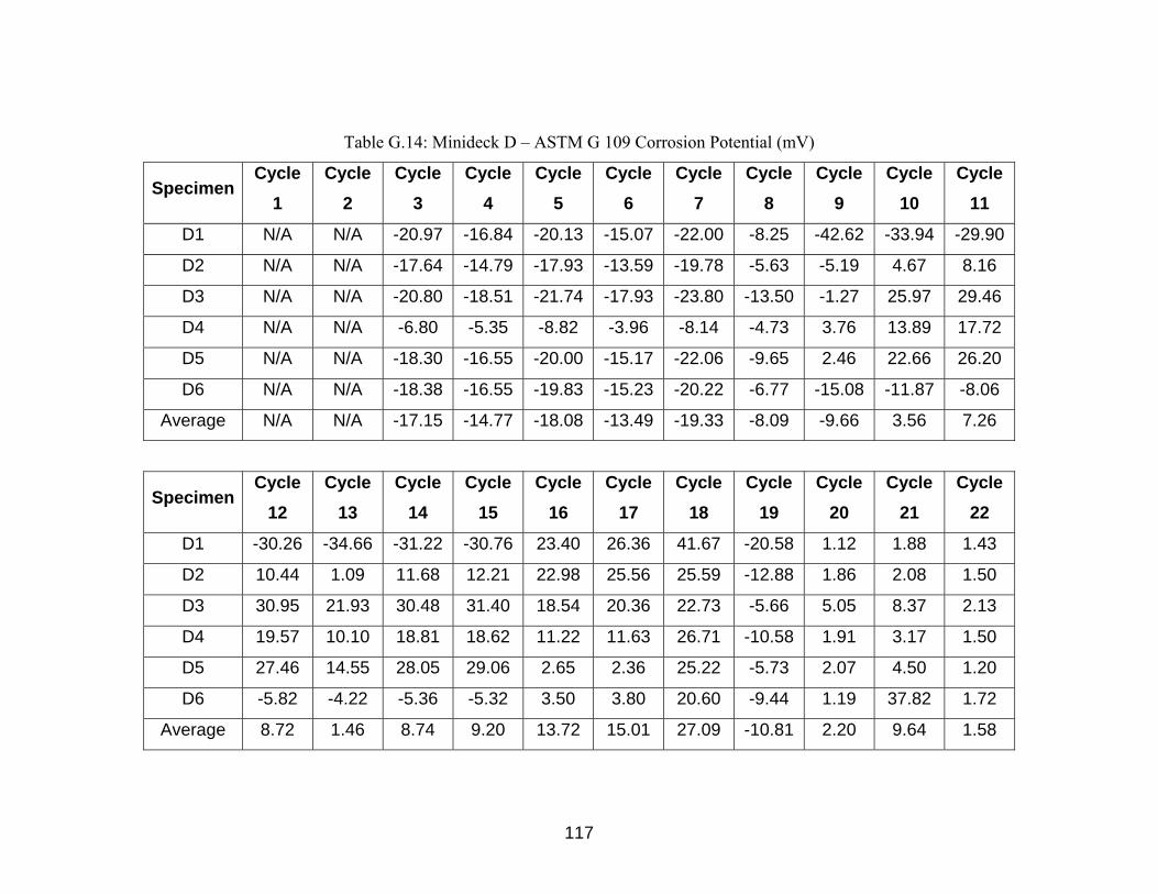
117
Table G.14: Minideck D – ASTM G 109 Corrosion Potential (mV)
Specimen Cycle
1 Cycle
2 Cycle
3 Cycle
4 Cycle
5 Cycle
6 Cycle
7 Cycle
8 Cycle
9 Cycle
10 Cycle
11
D1 N/A N/A -20.97 -16.84 -20.13 -15.07 -22.00 -8.25 -42.62 -33.94 -29.90
D2 N/A N/A -17.64 -14.79 -17.93 -13.59 -19.78 -5.63 -5.19 4.67 8.16
D3 N/A N/A -20.80 -18.51 -21.74 -17.93 -23.80 -13.50 -1.27 25.97 29.46
D4 N/A N/A -6.80 -5.35 -8.82 -3.96 -8.14 -4.73 3.76 13.89 17.72
D5 N/A N/A -18.30 -16.55 -20.00 -15.17 -22.06 -9.65 2.46 22.66 26.20
D6 N/A N/A -18.38 -16.55 -19.83 -15.23 -20.22 -6.77 -15.08 -11.87 -8.06
Average N/A N/A -17.15 -14.77 -18.08 -13.49 -19.33 -8.09 -9.66 3.56 7.26
Specimen Cycle
12 Cycle
13 Cycle
14 Cycle
15 Cycle
16 Cycle
17 Cycle
18 Cycle
19 Cycle
20 Cycle
21 Cycle
22
D1 -30.26 -34.66 -31.22 -30.76 23.40 26.36 41.67 -20.58 1.12 1.88 1.43
D2 10.44 1.09 11.68 12.21 22.98 25.56 25.59 -12.88 1.86 2.08 1.50
D3 30.95 21.93 30.48 31.40 18.54 20.36 22.73 -5.66 5.05 8.37 2.13
D4 19.57 10.10 18.81 18.62 11.22 11.63 26.71 -10.58 1.91 3.17 1.50
D5 27.46 14.55 28.05 29.06 2.65 2.36 25.22 -5.73 2.07 4.50 1.20
D6 -5.82 -4.22 -5.36 -5.32 3.50 3.80 20.60 -9.44 1.19 37.82 1.72
Average 8.72 1.46 8.74 9.20 13.72 15.01 27.09 -10.81 2.20 9.64 1.58

118
-30.00
-20.00
-10.00
0.00
10.00
20.00
30.00
0 1 2 3 4 5 6 7 8 9 10 11 12 13 14 15 16 17 18 19 20 21 22 23
Cycles
Cor
rosi
on P
oten
tial (
mV)
Fig. G.7: Minideck D – Average Corrosion Potential (mV)

119
Table G.15: Wyckoff Road Eastbound GECOR 6 Corrosion Rate (µA/cm2)
Connection #
Reading #
Cycle 1
Cycle 2
Cycle 3
Cycle 4
Cycle 5
Cycle 6
Cycle 7
Cycle 8
B1 1 0.038 0.146 0.257 0.071 0.052 0.212 0.317 0.297
2 0.048 0.118 0.249 0.092 0.192 0.077 0.272 0.121
3 0.033 0.089 0.214 0.210 0.272 0.178 0.199 0.244
4 0.168 0.125 0.168 0.150 0.422 0.134 0.222 0.307
5 0.153 0.198 0.283 0.092 0.042 0.079 0.212 0.199
B2 1 0.190 0.578 0.229 0.078 0.092 0.117 0.232 0.322
2 0.134 0.593 0.379 0.078 0.177 0.224 0.334 0.209
3 0.094 0.105 0.285 0.112 0.077 0.124 0.272 0.319
4 0.176 0.142 0.274 0.105 0.179 0.212 0.312 0.099
5 0.162 0.146 0.320 0.130 0.272 0.144 0.211 0.275
B3 1 0.135 0.106 0.314 0.142 0.155 0.167 0.044 0.272
2 0.096 0.120 0.356 0.066 0.212 0.052 0.313 0.212
3 0.110 0.083 0.198 0.134 0.137 0.144 0.232 0.372
4 0.126 0.132 0.234 0.062 0.071 0.123 0.054 0.109
5 0.200 0.179 0.195 0.043 0.121 0.321 0.091 0.262
B4 1 0.036 0.223 0.210 0.153 0.155 0.167 0.272 0.148
2 0.028 0.180 0.321 0.112 0.073 0.148 0.198 0.278
3 0.084 0.140 0.708 0.085 0.312 0.243 0.297 0.311
4 0.169 0.210 0.369 0.088 0.278 0.312 0.066 0.124
5 0.108 0.138 0.623 0.115 0.194 0.244 0.233 0.092
Average 0.114 0.188 0.309 0.106 0.174 0.171 0.219 0.229
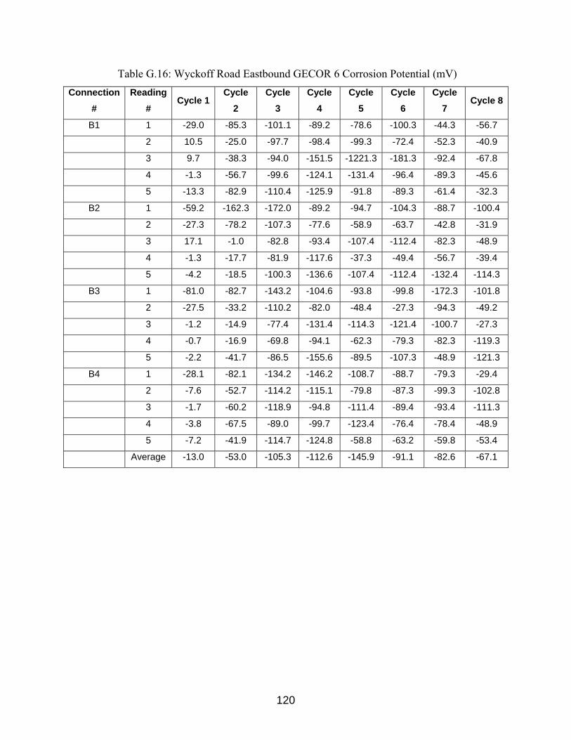
120
Table G.16: Wyckoff Road Eastbound GECOR 6 Corrosion Potential (mV) Connection
# Reading
# Cycle 1
Cycle 2
Cycle 3
Cycle 4
Cycle 5
Cycle 6
Cycle 7
Cycle 8
B1 1 -29.0 -85.3 -101.1 -89.2 -78.6 -100.3 -44.3 -56.7
2 10.5 -25.0 -97.7 -98.4 -99.3 -72.4 -52.3 -40.9
3 9.7 -38.3 -94.0 -151.5 -1221.3 -181.3 -92.4 -67.8
4 -1.3 -56.7 -99.6 -124.1 -131.4 -96.4 -89.3 -45.6
5 -13.3 -82.9 -110.4 -125.9 -91.8 -89.3 -61.4 -32.3
B2 1 -59.2 -162.3 -172.0 -89.2 -94.7 -104.3 -88.7 -100.4
2 -27.3 -78.2 -107.3 -77.6 -58.9 -63.7 -42.8 -31.9
3 17.1 -1.0 -82.8 -93.4 -107.4 -112.4 -82.3 -48.9
4 -1.3 -17.7 -81.9 -117.6 -37.3 -49.4 -56.7 -39.4
5 -4.2 -18.5 -100.3 -136.6 -107.4 -112.4 -132.4 -114.3
B3 1 -81.0 -82.7 -143.2 -104.6 -93.8 -99.8 -172.3 -101.8
2 -27.5 -33.2 -110.2 -82.0 -48.4 -27.3 -94.3 -49.2
3 -1.2 -14.9 -77.4 -131.4 -114.3 -121.4 -100.7 -27.3
4 -0.7 -16.9 -69.8 -94.1 -62.3 -79.3 -82.3 -119.3
5 -2.2 -41.7 -86.5 -155.6 -89.5 -107.3 -48.9 -121.3
B4 1 -28.1 -82.1 -134.2 -146.2 -108.7 -88.7 -79.3 -29.4
2 -7.6 -52.7 -114.2 -115.1 -79.8 -87.3 -99.3 -102.8
3 -1.7 -60.2 -118.9 -94.8 -111.4 -89.4 -93.4 -111.3
4 -3.8 -67.5 -89.0 -99.7 -123.4 -76.4 -78.4 -48.9
5 -7.2 -41.9 -114.7 -124.8 -58.8 -63.2 -59.8 -53.4
Average -13.0 -53.0 -105.3 -112.6 -145.9 -91.1 -82.6 -67.1
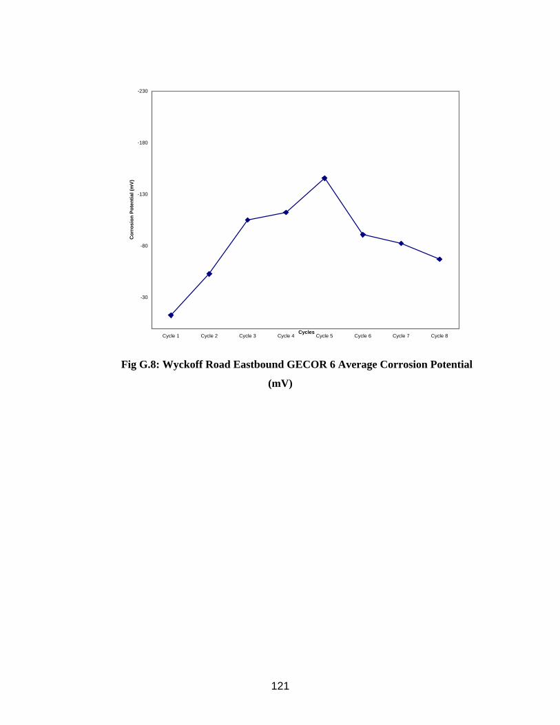
121
-230
-180
-130
-80
-30
Cycle 1 Cycle 2 Cycle 3 Cycle 4 Cycle 5 Cycle 6 Cycle 7 Cycle 8Cycles
Cor
rosi
on P
oten
tial (
mV)
Fig G.8: Wyckoff Road Eastbound GECOR 6 Average Corrosion Potential
(mV)
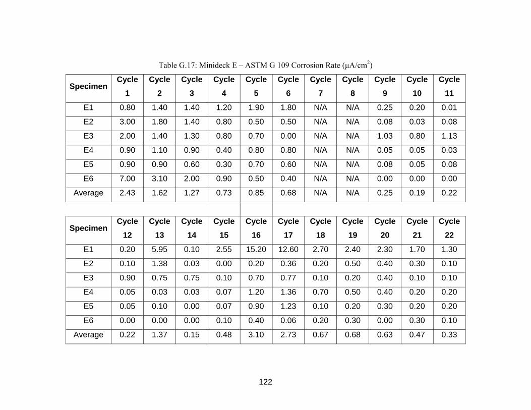
122
Table G.17: Minideck E – ASTM G 109 Corrosion Rate (µA/cm2)
Specimen Cycle
1 Cycle
2 Cycle
3 Cycle
4 Cycle
5 Cycle
6 Cycle
7 Cycle
8 Cycle
9 Cycle
10 Cycle
11
E1 0.80 1.40 1.40 1.20 1.90 1.80 N/A N/A 0.25 0.20 0.01
E2 3.00 1.80 1.40 0.80 0.50 0.50 N/A N/A 0.08 0.03 0.08
E3 2.00 1.40 1.30 0.80 0.70 0.00 N/A N/A 1.03 0.80 1.13
E4 0.90 1.10 0.90 0.40 0.80 0.80 N/A N/A 0.05 0.05 0.03
E5 0.90 0.90 0.60 0.30 0.70 0.60 N/A N/A 0.08 0.05 0.08
E6 7.00 3.10 2.00 0.90 0.50 0.40 N/A N/A 0.00 0.00 0.00
Average 2.43 1.62 1.27 0.73 0.85 0.68 N/A N/A 0.25 0.19 0.22
Specimen Cycle
12 Cycle
13 Cycle
14 Cycle
15 Cycle
16 Cycle
17 Cycle
18 Cycle
19 Cycle
20 Cycle
21 Cycle
22
E1 0.20 5.95 0.10 2.55 15.20 12.60 2.70 2.40 2.30 1.70 1.30
E2 0.10 1.38 0.03 0.00 0.20 0.36 0.20 0.50 0.40 0.30 0.10
E3 0.90 0.75 0.75 0.10 0.70 0.77 0.10 0.20 0.40 0.10 0.10
E4 0.05 0.03 0.03 0.07 1.20 1.36 0.70 0.50 0.40 0.20 0.20
E5 0.05 0.10 0.00 0.07 0.90 1.23 0.10 0.20 0.30 0.20 0.20
E6 0.00 0.00 0.00 0.10 0.40 0.06 0.20 0.30 0.00 0.30 0.10
Average 0.22 1.37 0.15 0.48 3.10 2.73 0.67 0.68 0.63 0.47 0.33

123
Table G.18: Minideck E – ASTM G 109 Corrosion Potential (mV)
Specimen Cycle
1 Cycle
2 Cycle
3 Cycle
4 Cycle
5 Cycle
6 Cycle
7 Cycle
8 Cycle
9 Cycle
10 Cycle
11
E1 -94.32 -73.40 -66.60 -55.86 -62.34 -38.95 N/A N/A 8.78 12.61 16.22
E2 -7.97 -64.68 -53.10 -39.54 -45.07 -18.83 N/A N/A -12.15 -3.34 0.67
E3 -62.93 -46.52 -42.77 -33.97 -40.54 -22.73 N/A N/A -21.28 -13.70 -10.08
E4 -73.88 -53.66 -48.76 -41.68 -50.61 -32.22 N/A N/A -14.53 -6.00 -1.14
E5 -79.75 -56.92 -51.90 -43.13 -50.35 -30.42 N/A N/A -17.51 -13.95 -10.30
E6 -110.5 -77.53 -70.85 -52.01 -55.15 -33.19 N/A N/A -1.72 -10.8 0.15
Average -84.90 -62.12 -55.66 -44.37 -50.68 -29.39 N/A N/A -9.74 -5.86 -0.75
Specimen Cycle
12 Cycle
13 Cycle
14 Cycle
15 Cycle
16 Cycle
17 Cycle
18 Cycle
19 Cycle
20 Cycle
21 Cycle
22
E1 17.84 11.73 20.35 22.85 3.32 3.36 13.28 3.44 1.21 50.64 2.28
E2 2.49 -0.48 2.95 2.10 3.25 3.45 22.90 -9.72 1.65 9.81 3.55
E3 -8.10 -16.21 -8.09 -8.18 18.00 20.00 16.62 -1.71 1.46 6.88 3.92
E4 0.84 -8.68 1.74 2.08 2.42 3.60 10.75 4.36 2.18 7.50 0.92
E5 -8.24 -12.45 -8.72 -8.37 13.18 14.58 14.12 -0.06 1.90 18.38 0.89
E6 5.67 -0.01 -0.91 -5.32 18.25 19.36 11.45 2.92 0.98 7.33 1.44
Average 1.75 -4.35 1.22 0.86 9.74 10.73 14.85 -0.13 1.56 16.76 2.17
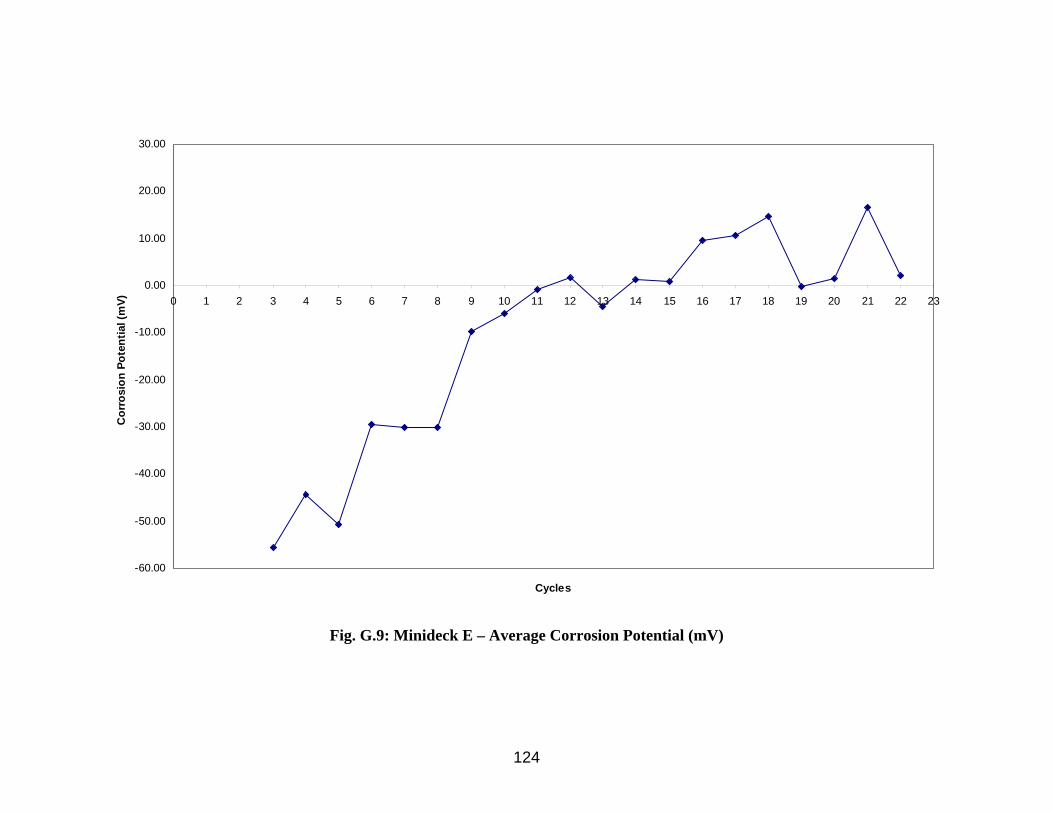
124
-60.00
-50.00
-40.00
-30.00
-20.00
-10.00
0.00
10.00
20.00
30.00
0 1 2 3 4 5 6 7 8 9 10 11 12 13 14 15 16 17 18 19 20 21 22 23
Cycles
Cor
rosi
on P
oten
tial (
mV)
Fig. G.9: Minideck E – Average Corrosion Potential (mV)
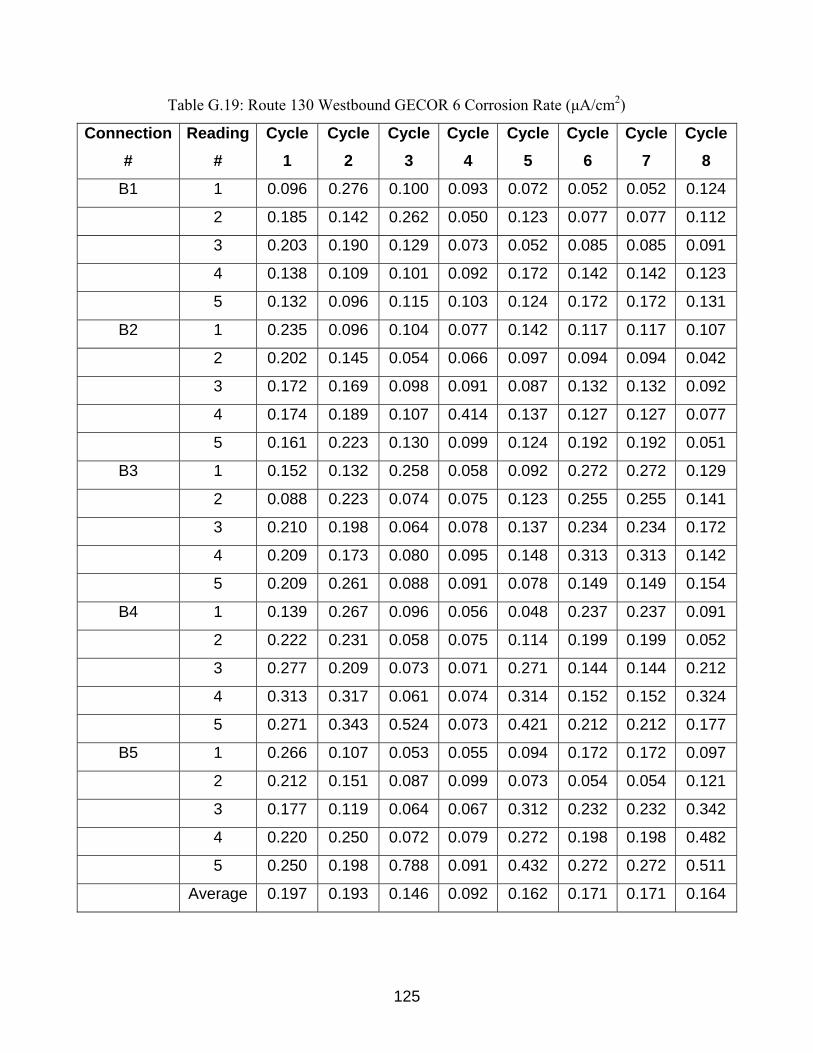
125
Table G.19: Route 130 Westbound GECOR 6 Corrosion Rate (µA/cm2)
Connection #
Reading #
Cycle 1
Cycle 2
Cycle 3
Cycle 4
Cycle 5
Cycle 6
Cycle 7
Cycle 8
B1 1 0.096 0.276 0.100 0.093 0.072 0.052 0.052 0.124
2 0.185 0.142 0.262 0.050 0.123 0.077 0.077 0.112
3 0.203 0.190 0.129 0.073 0.052 0.085 0.085 0.091
4 0.138 0.109 0.101 0.092 0.172 0.142 0.142 0.123
5 0.132 0.096 0.115 0.103 0.124 0.172 0.172 0.131
B2 1 0.235 0.096 0.104 0.077 0.142 0.117 0.117 0.107
2 0.202 0.145 0.054 0.066 0.097 0.094 0.094 0.042
3 0.172 0.169 0.098 0.091 0.087 0.132 0.132 0.092
4 0.174 0.189 0.107 0.414 0.137 0.127 0.127 0.077
5 0.161 0.223 0.130 0.099 0.124 0.192 0.192 0.051
B3 1 0.152 0.132 0.258 0.058 0.092 0.272 0.272 0.129
2 0.088 0.223 0.074 0.075 0.123 0.255 0.255 0.141
3 0.210 0.198 0.064 0.078 0.137 0.234 0.234 0.172
4 0.209 0.173 0.080 0.095 0.148 0.313 0.313 0.142
5 0.209 0.261 0.088 0.091 0.078 0.149 0.149 0.154
B4 1 0.139 0.267 0.096 0.056 0.048 0.237 0.237 0.091
2 0.222 0.231 0.058 0.075 0.114 0.199 0.199 0.052
3 0.277 0.209 0.073 0.071 0.271 0.144 0.144 0.212
4 0.313 0.317 0.061 0.074 0.314 0.152 0.152 0.324
5 0.271 0.343 0.524 0.073 0.421 0.212 0.212 0.177
B5 1 0.266 0.107 0.053 0.055 0.094 0.172 0.172 0.097
2 0.212 0.151 0.087 0.099 0.073 0.054 0.054 0.121
3 0.177 0.119 0.064 0.067 0.312 0.232 0.232 0.342
4 0.220 0.250 0.072 0.079 0.272 0.198 0.198 0.482
5 0.250 0.198 0.788 0.091 0.432 0.272 0.272 0.511
Average 0.197 0.193 0.146 0.092 0.162 0.171 0.171 0.164
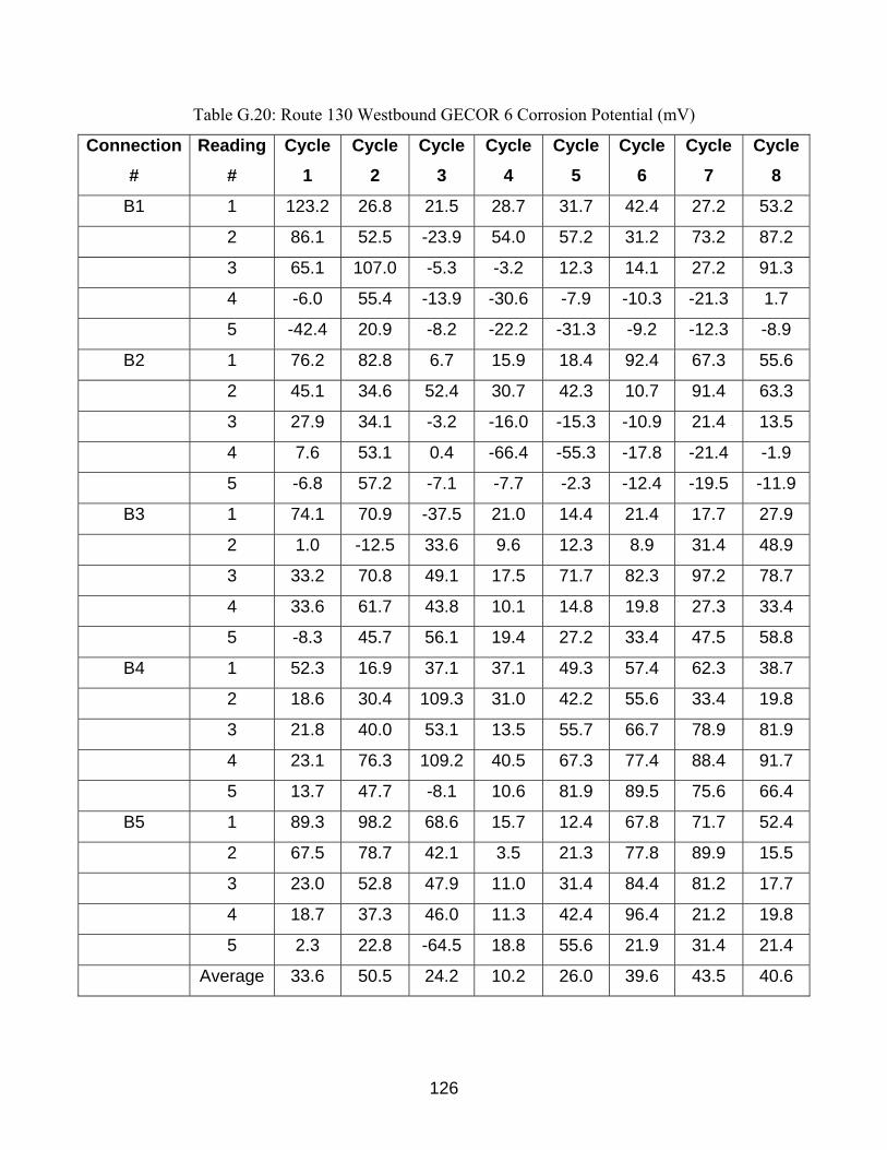
126
Table G.20: Route 130 Westbound GECOR 6 Corrosion Potential (mV)
Connection #
Reading #
Cycle 1
Cycle 2
Cycle 3
Cycle 4
Cycle 5
Cycle 6
Cycle 7
Cycle 8
B1 1 123.2 26.8 21.5 28.7 31.7 42.4 27.2 53.2
2 86.1 52.5 -23.9 54.0 57.2 31.2 73.2 87.2
3 65.1 107.0 -5.3 -3.2 12.3 14.1 27.2 91.3
4 -6.0 55.4 -13.9 -30.6 -7.9 -10.3 -21.3 1.7
5 -42.4 20.9 -8.2 -22.2 -31.3 -9.2 -12.3 -8.9
B2 1 76.2 82.8 6.7 15.9 18.4 92.4 67.3 55.6
2 45.1 34.6 52.4 30.7 42.3 10.7 91.4 63.3
3 27.9 34.1 -3.2 -16.0 -15.3 -10.9 21.4 13.5
4 7.6 53.1 0.4 -66.4 -55.3 -17.8 -21.4 -1.9
5 -6.8 57.2 -7.1 -7.7 -2.3 -12.4 -19.5 -11.9
B3 1 74.1 70.9 -37.5 21.0 14.4 21.4 17.7 27.9
2 1.0 -12.5 33.6 9.6 12.3 8.9 31.4 48.9
3 33.2 70.8 49.1 17.5 71.7 82.3 97.2 78.7
4 33.6 61.7 43.8 10.1 14.8 19.8 27.3 33.4
5 -8.3 45.7 56.1 19.4 27.2 33.4 47.5 58.8
B4 1 52.3 16.9 37.1 37.1 49.3 57.4 62.3 38.7
2 18.6 30.4 109.3 31.0 42.2 55.6 33.4 19.8
3 21.8 40.0 53.1 13.5 55.7 66.7 78.9 81.9
4 23.1 76.3 109.2 40.5 67.3 77.4 88.4 91.7
5 13.7 47.7 -8.1 10.6 81.9 89.5 75.6 66.4
B5 1 89.3 98.2 68.6 15.7 12.4 67.8 71.7 52.4
2 67.5 78.7 42.1 3.5 21.3 77.8 89.9 15.5
3 23.0 52.8 47.9 11.0 31.4 84.4 81.2 17.7
4 18.7 37.3 46.0 11.3 42.4 96.4 21.2 19.8
5 2.3 22.8 -64.5 18.8 55.6 21.9 31.4 21.4
Average 33.6 50.5 24.2 10.2 26.0 39.6 43.5 40.6
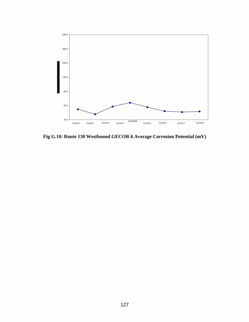
127
-230.0
-180.0
-130.0
-80.0
-30.0
20.0
70.0 Cy c l e sCycle 1 Cycle 2 Cycle 3 Cycle 4 Cycle 5 Cycle 6 Cycle 7 Cycle 8
Fig G.10: Route 130 Westbound GECOR 6 Average Corrosion Potential (mV)