evaluation of continuous green t-intersections on …docs.trb.org/prp/13-0591.pdf1 evaluation of...

Evaluation of Continuous Green T-Intersections on 1

Isolated Under-Saturated Four-Lane Highways 2

3 4 Stephen Litsas 5 Arup 6 560 Mission Street 7 Suite 700 8 San Francisco, California, USA 94105 9 Ph: (415) 957-9445 10 Email: [email protected] 11 12 13 Hesham Rakha, Ph.D., P.Eng. (Corresponding Author) 14 Charles E. Via, Jr. Department of Civil and Environmental Engineering, Virginia Tech 15 Virginia Tech Transportation Institute 16 3500 Transportation Research Plaza 17 Blacksburg, Virginia, USA 24061 18 Ph: (540) 231-1505 19 Fax: (540) 231-1555 20 Email: [email protected] 21 22 23 24 25 26 A paper prepared for the Transportation Research Board 2013 Annual Meeting 27 Number of words in text: 5,772 28 Number of figures and tables: 6 (1,500) 29 Total word count: 7,272 30 31 July, 2012 32

TRB 2013 Annual Meeting Paper revised from original submittal.

Litsas and Rakha 2

Abstract 33

The research presented in this paper analyzes the merging version of the Continuous Green T-Intersection 34 (CGT), an alternative intersection design/control that allows certain lanes along the main street to bypass 35 three-way intersections, with side-street traffic merging onto the main road. A comprehensive model 36 encompassing 2,445 unique intersection condition combinations was run, comparing the merging CGT to 37 the standard three-way signalized intersection. The study demonstrated significant intersection 38 improvements compared to conventional traffic signal timing. Specifically, significant benefits were 39 observed for the merging CGT in terms of total delay, fuel usage, hydrocarbon, carbon monoxide, oxides 40 of nitrogen, and carbon dioxide emissions. Additionally, an economic analysis showed significant user 41 savings associated with CGT control. Due to the higher traffic volumes of the main road versus the side-42 street, savings for main-street vehicles outweighed any dis-benefits associated with side street traffic 43 merging into the main street flow. These findings strongly support the decision to implement the merging 44 CGT over standard three-way signalized intersection control. Prior to this work, no comprehensive model 45 has been published that considers the environmental and economic implications of any form of the CGT, 46 nor is there a comprehensive model that specifically focuses on the merging version of the CGT. 47


Litsas and Rakha 3

Introduction 48

Throughout America’s road network, numerous miles of four-lane highways span our states, many of 49 which require three-way signalized intersections. An alternative intersection design, entitled Continuous 50 Green T-Intersection (CGT), creates an ideal alternative to the standard three-way signalized intersection 51 by isolating one approach so it can continuously bypass the signal, significantly improving the 52 intersection performance. 53 There are two types of CGT designs: traditional version and merging version. The traditional 54 CGT requires some lanes in the continuous direction to be signalized while others can freely pass the 55 intersection. Vehicles within these signalized lanes stop to allow left-turners from the side-street to enter 56 lanes directly when turning onto the main thoroughfare, whereas the other lanes in the same direction not 57 needed to intercept left-turners are allowed to continually bypass the intersection. The merging CGT 58 allows all lanes in the continuous direction to bypass the signal, with left turners from the side street being 59 required to merge onto the main-thoroughfare, in the same fashion that a vehicle would merge onto a 60 highway. The merging CGT provides similar efficiency benefits to the traditional CGT, yet reduces driver 61 confusion and improves safety. 62

This paper compares the merging version of the CGT to the standard three-way signalized 63 intersection, analyzing the sustainable costs and benefits that can be expected by implementing this type 64 of intersection control. While some limited research has been conducted on the traditional CGT, which 65 has existed in Florida for many years, there are no comprehensive studies that evaluate the performance 66 of the merging CGT and compare it to standard signalized intersection control. Prior to this research, no 67 comprehensive model involving any form of the CGT has analyzed the performance of this intersection 68 from a sustainability perspective, considering both the environmental and economic implications of 69 implementation. To date, only minor case studies partially consider the sustainable aspects of the 70 traditional CGT. 71

Commonly Used Terms 72 The following terms will be used throughout this paper: 73

• Continuous-Green Version/Design: The intersection model that the standard version will be 74 compared against. Shown pictorially in Figure 1, this is considered to be an alternative 75 intersection design-type that inserts continuous lanes into a T-intersection. 76

• Continuous side: The side of the main-thoroughfare opposite of the side-street. In the continuous-77 green version, this will be the side of the road that is converted to continuous lanes. The opposite 78 side of the road will be the non-continuous side. 79

• Main-thoroughfare: The road that continues through the intersection in both directions. 80 • Side-street: The side-street that intersects the main-thoroughfare. 81 • Standard Version/Design: The intersection type that is considered the “common” design for 82

signalized T-intersections. A pictorial example of this intersection type can be seen in Figure 1. 83 • Main Vehicle Movement (Main-VM): The grouping of vehicles that proceed through the main-84

thoroughfare along the continuous side of the intersection. In the continuous-green version, these 85 will be the vehicles that utilize the continuous lanes. 86

• Side Vehicle Movement (Side-VM): The grouping of vehicles that make a left-turn from the side-87 street onto the main-thoroughfare. In the continuous-green version, these will be the vehicles that 88 will merge into the continuous lanes. 89

Literature Review 90 There are five reports done by academia, government, and the private sector that can be attributed to the 91 base of research knowledge for the CGT. All five of these focus on the traditional CGT, not on the 92


Litsas and Rakha 4

merging CGT. However, many of their conclusions may be appropriate for both the traditional CGT and 93 merging CGT designs: 94

• Boone and Hummer [1] modeled many alternative intersection designs, thoroughly comparing 95 them in terms of intersection delay, with the traditional CGT design being one of the alternative 96 intersections studied. The traditional CGT yielded positive results when compared with other 97 three-way at-grade intersection designs. However, because this report only compares in terms of 98 delay time and does not look at the merging CGT, it leaves some room for improved research. 99

• Jarem [2] compared the features of five Florida traditional CGT intersections, considering the 100 costs and benefits of the installation of each intersection. This was a well developed case-study 101 that showed delay improvements and economic benefits found with the traditional CGT design; 102 however, five intersections provides for a narrow scope. 103

• Reid [3] performed a traditional CGT literature review and compiled the information, only adding 104 an interview with a Florida DOT engineer who confirmed the positive benefits of the design to 105 the base of the research knowledge. 106

• Rice and Znamenacek [4] published a FHWA safety-report that case-studies two traditional CGT 107 designs, evaluating their safety improvements over the previous standard intersection control. The 108 report stated very positive safety benefits of the design; however, conclusions were formed 109 through a very narrow scope of analysis and did not consider other intersection performance 110 aspects. 111

• Sando et al [5] investigated crash-data for nine Florida traditional CGT’s, comparing the safety of 112 each intersection. The results showed very positive safety improvements for the design, but did 113 not evaluate other intersection performance aspects. 114

115 Additionally, some papers that helped shaped the framework for conducting this research: 116

• Park and Rakha [6] used similar methodology to this research to analyze the environmental 117 impacts of four-legged Continuous Flow Intersections. 118

• El Esawey and Sayed [7] discuss methodologies that should be utilized when modeling four-119 legged unconventional intersection designs. 120

121

Scope of Research 122 The purpose of this research is to analyze the sustainable benefits and costs that can be expected from the 123 implementation of the merging Continuous Green T-Intersection (CGT) control versus the standard three-124 way signalized intersection control. Sustainability, a term commonly used synonymously with 125 environmental consideration, entails considering the economic, environmental, and social dimensions of a 126 design holistically. For this model, the economic and environmental impacts will be quantified and 127 potential social impacts will be briefly discussed. 128

In particular, the research effort presented in this paper quantifies the improvement that can be 129 seen by converting traditional lanes to continuous lanes in a three-way intersection. The model will 130 compare the standard three-way intersection design (called the “standard” version henceforth) versus the 131 merging CGT design (called the “continuous-green” version henceforth). The modeling software, 132 INTEGRATION, will compute the differences for the following six analyzed categories between both 133 designs: total delay, fuel consumption, hydrocarbon (HC), carbon monoxide (CO), Oxides of Nitrogen 134 (NOx), and carbon dioxide (CO2) emissions. After determining total delay and fuel usage, a user time cost 135 and fuel cost can be applied, which will determine the economic costs/benefits of implementing the 136 merging CGT design. 137

Figure 1 provides a pictorial representation of the two intersections that will be modeled and the 138 accompanying signal phasing scheme. 139


Litsas and Rakha 5

140 Figure 1: Standard design versus Continuous Green design. Top: Plan view of intersection. Bottom: Signal 141

phasing scheme (Note: Common arrows between adjacent phases does not infer overlapping signal phases; they 142 are shown for illustration purposes only) 143

STANDARD VERSION

CONTINUOUS GREEN VERSION

CONTINUOUS GREEN VERSION:

STANDARD VERSION:


Litsas and Rakha 6

Variables 144 To create a comprehensive scope of the merging CGT, the following five factors were varied and 145 simulated: 146

• (v/s)thru [Varied values: 0.40, 0.50, 0.60, 0.70, and 0.80] –This represents the volume/saturation 147 ratio for the approach lanes of the main-thoroughfare upstream of the intersection. 148

• (v/s)side [Varied values: 0.05, 0.10, 0.15, 0.20, 0.25] – This represents the volume/saturation ratio 149 for the approach lane of the side-street upstream of the intersection. 150

• (% turners)thru [Varied values: 5.0, 15.0, 25.0, 35.0, 45.0%] – This represents the percentage of 151 total approach arrivals that turn from the main-thoroughfare onto the side-street. This percentage 152 is determined as a percent of the upstream volume, calculated from the (v/s)thru ratio. On the 153 “continuous” side of the road, this will be left-hand turners. On the “non-continuous” side of the 154 road, this will be right-hand turners. 155

• (% left turners)side [Varied values: 20.0, 40.0, 50.0, 60.0, 80.0%]– This represents the percentage 156 of vehicles from the side-street that turn left onto the main-thoroughfare. The drivers not 157 accounted for turning left will by default be turning right. 158

• (speed limit) [Varied values: 35.0, 45.0, 55.0, 60.0, 65.0 mph] – This represents be the speed limit 159 of the main-thoroughfare and side-street, as defined in miles per hour (mph). In order to keep the 160 same speed throughout the model, the speed-at-capacity will be the same as the posted speed limit 161 (i.e. considering a Pipes car-following model). 162

These combination of all factors resulted in a total of 3,125 different possible cases to be modeled. 163 However, 680 cases over-saturated the intersection and thus not were optimizable under the chosen 164 methodology, leaving a total of 2,445 cases modeled in both the standard and continuous-green designs. 165

Constants 166 Factors not listed as one of the five variables or mentioned below were maintained constant throughout 167 the simulations. 168

• A saturation flow rate of 1800 veh/h/lane was used for all lanes. 169 • The main-thoroughfare was considered to be a four-lane road, with two lanes running in each 170

direction. The approach volume was assigned based upon the (v/s)thru ratio for these four lanes. 171 Additional lanes were added as follows: 172

o One left-turn lane from the main-thoroughfare on the continuous side of the road, which 173 was kept at an ample lane length such that cars queuing to turn left would not spillback 174 onto the continuous lanes. 175

o In the continuous-green version, an acceleration lane for left-turners from the side-street 176 was added. In order to model realistic situations, the length of this lane varied based upon 177 the given speed limit for each test scenario, and was computed using the standards set in 178 the Texas DOT 2010 Roadway Design Manual, Chapter 3, Figure 3-36 [8]. 179

o A deceleration lane for right turners from the non-continuous side of the intersection. 180 This lane length is the same length as the acceleration lane in the continuous-green 181 version, or computed based on the speed limit for a standard intersection. 182

• The side-street was considered to be a two-lane road, with one lane designated for each direction. 183 The volume approaching the intersection was determined by the (v/s)side ratio. As the single lane 184 approached the intersection, it was split into a right-turn lane and left-turn lane, with the 185 appropriate volume entering the appropriate lane. 186

• The traffic demand was discharged for 600 seconds and the simulation was run to ensure that all 187 vehicles completed their trip. 188

• All origin and destination nodes were exactly 2 km away from the intersection, thus each vehicle 189 traveled 4 km. This upstream and downstream distance was chosen to ensure all vehicles would 190


Litsas and Rakha 7

be continuously monitored in heavy delay situations. In INTEGRATION, vehicle emissions are 191 only recorded while vehicles are traveling between the origin and destination nodes. 192

• Signal timings were optimized for every case, following the phasing scheme shown in Figure 1. 193 Because converted lanes are not critical lanes for optimizing the signal, the signal timings were 194 the same for identical run conditions in both cases. In actuality, the traffic in the continuous lanes 195 for the continuous-green design did not cross through a signal when passing through the 196 intersection, but for the purposes of running the model, the phasing scheme shows the continuous 197 lanes always given a green light. No permissive left-turn movements were allowed in any 198 direction in the model. 199

Limitations 200 The safety implications (both positive and negative) of the continuous-green version versus the standard 201 version are not analyzed in this study. Many of the conflict zones within the traditional CGT design are 202 significantly reduced by using the merging version of the CGT. Furthermore, there are recent published 203 studies that look at the safety factors of the traditional CGT model [5], encompassing a majority of the 204 conflict zones that remain within the merging CGT model. An additional conflict zone would be created 205 by introducing merging lanes onto the main-thoroughfare, but this conflict could be similar to that on a 206 typical interstate highway. 207

The analysis only considered an isolated intersection because of certain underlying factors in non-208 isolated intersections that will need further analysis. The conflicts of nearby intersections and pedestrians 209 crossing the continuous lanes could have significant effects on the performance of the merging CGT. In 210 isolated areas, it is assumed that there are no other intersections or pedestrians near the CGT. 211

This analysis only looks at under-saturated conditions; over-saturated conditions present a 212 different set of parameters and conditions that should be looked at in future research. Oversaturated 213 conditions were not analyzed because they could not be optimized as the equations did not allow an 214 optimum cycle length to be determined. Additionally, if vehicles were continually discharged at an 215 oversaturated rate, it would produce an increasingly larger delay that would not decrease until the origin 216 node stopped discharging vehicles, which would then unrealistically decrease the delay. Towards the end 217 of the model running in oversaturated conditions, vehicles would continue to process through the 218 intersection in the oversaturated directions, but no longer in the undersaturated directions, affecting the 219 delay time seen from merging vehicles. It is not possible to stop the model prior to all vehicles being 220 received at the destination nodes, as vehicle data is only recorded once a vehicle hits its final destination. 221 Therefore, only 2,445 of the 3,125 possible run conditions were examined. 222

Modeling Software 223 INTEGRATION was the software used for this analysis. INTEGRATION software is a microscopic 224 traffic assignment and simulation software, developed within the past decade, that was conceived as an 225 integrated simulation and traffic assignment model to perform traffic simulations by tracking the 226 movement of individual vehicles every 1/10th of a second. This allows detailed analyses of lane-changing 227 movements and shock wave propagations. It also permits considerable flexibility in representing spatial 228 and temporal variations in traffic conditions. In addition to estimating stops and delays, the model use 229 second-by-second speed and acceleration data in conjunction with microscopic fuel consumption and 230 emission models are used to estimate a vehicle’s instantaneous fuel consumption and emission rate [9]. 231 The INTEGRATION software is the only software that the authors are aware of that uses vehicle 232 dynamics to ensure that vehicle accelerations are realistic. The INTEGRATION model computes a 233 number of measures of effectiveness, including the network efficiency. Efficiency evaluation of highway 234 alternatives involves computing the average speed and vehicle delay. The instantaneous delay incurred by 235 a vehicle over a given interval can be estimated as the difference between the time it would take the 236 vehicle to complete its trip while traveling at the free-flow speed of the facility and the time the vehicle 237


Litsas and Rakha 8

actually took. This model has been validated against state-of-the-art delay estimation procedures using 238 queuing theory and shockwave analysis [10]. The software was selected for the study because it has been 239 extensively tested and validated over the past decade. 240

Methodology 241

1. A base intersection model was created, representing the standard version of the intersection 242 2. 3,125 different possible run conditions were created. 243 3. For each run condition, the signal timing for the intersection was optimized using Webster’s 244

optimum cycle length formula [11]. For each optimized cycle length, green times were allocated 245 based upon the Highway Capacity Manual 2000 method [12]. Optimization and allocation were 246 done automatically within Microsoft Excel, utilizing the VBA and Solver tools. 247

4. These run conditions were modeled in INTEGRATION for the base intersection model. Data for 248 each vehicle passing through the model was recorded. 249

5. A merging CGT intersection model was created and the identical run conditions were modeled 250 once again within this new model. 251

6. The results for identical run conditions were compared against each other, analyzed for Main-VM 252 and Side-VM. Because of intersection similarities between designs, these were the only two 253 vehicle movements that varied between the standard version and the merging version. A paired t-254 test was run for the six analyzed categories, utilizing a 95% confidence interval. A probability 255 density function and cumulative density function were also created for each result to visually 256 compare the results. 257

7. For tests that yielded confident results, an average per analyzed category for all vehicles within 258 that run condition was recorded, giving a total of 2,445 standard design averages and 2,445 259 continuous-green design averages. 260

8. Using the total delay and fuel consumption, an economic analysis was conducted. 261 9. Conclusions and recommendations were formulated. 262

Study Results 263

The Main-VM and Side-VM were the only two vehicle movements affected when converting from 264 standard intersection control to the merging CGT design, with the Main-VM greatly benefiting from 265 bypassing the intersection and Side-VM showing some dis-improvement from having to merge; therefore, 266 only Main-VM and Side-VM are discussed in the study results. 267

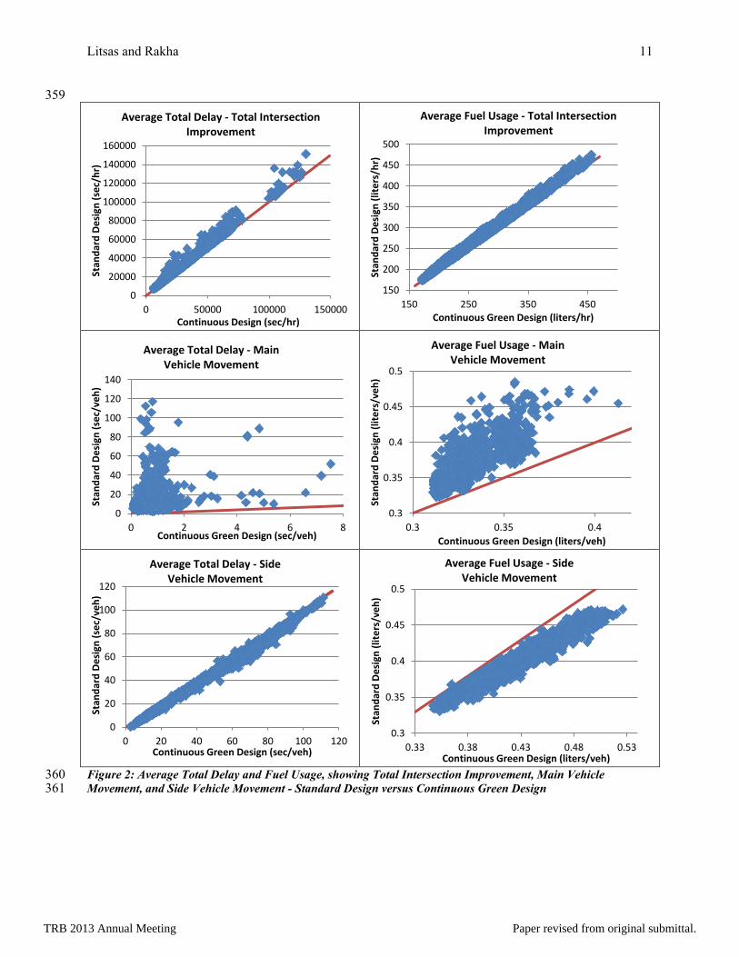
Total Delay 268 The total delay saw an overall average intersection improvement of 18,242 seconds per hour, which 269 equates to a 9.86% reduction. See Figure 2 for a graphical representation of the overall average 270 intersection improvement for total delay. 271

Main Vehicle Movement 272 Main-VM showed a reduction in total delay over all cases, with only 1 case being removed from the 273 analysis for having a paired-t value greater than 0.05. The total delay showed some variability in terms of 274 the actual reduction between cases, mostly based upon the amount of delay that was seen in the standard 275 version of the test. The average total delay per vehicle in the standard version showed most cases fell 276 between 4s and 60s, with an average between all cases being 11.41s. Most tests saw total delay in the 277 continuous-green version between 0s and 2s per vehicle, with a 0.68s average between all cases. This 278


Litsas and Rakha 9

yields a 94.0% reduction in delay between the two designs, agreeing with what was to be expected from 279 the research. 280 The five varied factors had the following effect on total delay: 281

• (v/s)thru – The reduction in delay per vehicle was much greater with higher volumes. For 0.4 282 versus 0.8, there was an average reduction of 8.16s versus 14.46s per vehicle, respectively. A 283 higher volume on the main-thoroughfare creates a longer delay when the red light is displayed 284 due to the additional start-up time seen with higher queued traffic. 285

• (v/s)side – An increase in side-street traffic showed a larger total delay reduction between designs. 286 For 0.05 versus 0.25, there was a 9.91s versus 11.98s average reduction per vehicle. 287

• (% turners)thru – The percentage of turners from the main-thoroughfare to the side-street did not 288 show any linear trends in total delay reduction. At 5% and 45%, there was a 12.00s and 16.39s 289 per vehicle average reduction, respectively, yet at 25% turners, a 7.90s reduction. 290

• (% left turners)side – Total delay reduction was slightly higher with a higher percent of left-291 turners. 292

• (speed limit) – A higher speed limit created a larger reduction in delay for Main-VM, which 293 would be expected by the additional time needed to decelerate and accelerate to and from a stop. 294 For 35 mph versus 65 mph, there was a 8.68s versus 11.96s average reduction in delay. 295

Side Vehicle Movement 296 Side-VM did not show a significant increase or decrease in total delay when averaged over all cases. Due 297 to the low traffic volumes modeled in many of the cases, only 1,600 of the 2,445 cases provided a paired-t 298 value of less than 0.05. This was due to there not being a high enough modeled volume to provide 299 confidence in these results. For this vehicle movement, there was expected to be little to no increase in the 300 total delay caused by additional merging. Including all cases, regardless of the paired-t confidence value, 301 the average total delay per vehicle in the standard version was 38.9s and in the continuous-green version 302 was 42.0s, leading to a 7.4% increase in delay time for Side-VM. None of the five varied factors had a 303 significant impact on the results. 304

Figure 2 compares the average total delay of the standard design versus the continuous-green 305 design for Main-VM and Side-VM. For each test, any point falling on the “Standard Design” side of the 306 1-to-1 ratio shows that the standard design yielded a higher total delay than the continuous-green design. 307 Likewise, any point falling on the “Continuous Green Design” side of the 1-to-1 ratio shows that the 308 continuous-green design yielded a higher total delay compared to the standard design. 309

Fuel Consumption/Carbon Dioxide Emissions 310 Fuel consumption and CO2 emissions have a proportional relationship, with 1L of fuel equating to 311 roughly 2,260g of CO2 emissions. The results saw an average overall intersection improvement of 54.1L 312 of fuel saved per hour (99,376g CO2), equating to a 2.78% reduction. The significance in fuel usage 313 reduction may be under shadowed by the amount of fuel needed to drive 4 km throughout the model, 314 which consumes the majority of the fuel used within the model. 315

Main Vehicle Movement 316 The significant reduction in total delay for Main-VM also resulted in a significant reduction in fuel usage 317 over all cases, with 2 cases being removed from the analysis for having a paired-t value greater than 0.05. 318 The average fuel usage for vehicles in the standard version showed most cases between the range of 319 0.33L and 0.45L (745g and 1000g CO2) per vehicle, with an average between all cases being 0.367L 320 (828.1g CO2). Most tests saw fuel usage in the continuous-green version between 0.31L and 0.37L (700g 321 and 835g CO2) per vehicle, with an average between all cases at 0.331L (762.8g CO2). This 9.8% 322 reduction in fuel usage is consistent with the delay reductions reported earlier. 323

The five varied factors had the following effect on fuel usage: 324


Litsas and Rakha 10

• (v/s)thru – A more significant reduction in fuel usage per vehicle with higher volumes on the main-325 thoroughfare versus low volumes. With 0.4 versus 0.8, an average reduction of 0.0367L versus 326 0.335L per vehicle occurred, respectively. 327

• (v/s)side – No statistical effect. 328 • (% turners)thru – The percent of main-thoroughfare turners had an interesting effect on fuel usage, 329

with 5% and 45% turners having the highest average reduction (0.0406L and 0.0424L, 330 respectively) and 25% turners having the lowest average reduction (0.0300L). 331

• (% left turners)side – No statistical effect. 332 • (speed limit) – This was the most noticeable impact on fuel usage. At 35 mph versus 65 mph, 333

there was an average 0.0157L versus 0.0531L per vehicle reduction, respectively, with the 334 reduction in fuel increasing linearly with an increase in the speed limit. 335

Side Vehicle Movement 336 Side-VM showed a slight increase in fuel usage between designs. Of the 2,445 conditions examined, 337 2,033 had a paired-t value less than 0.05 and were considered statistically significant. The average fuel 338 usage for vehicles in the standard version showed most cases between 0.33L and 0.47L (745g and 1060g 339 CO2) per vehicle, with an average between all cases being 0.392L (872.7g CO2). Most tests saw fuel 340 usage in the continuous-green version between 0.35L and 0.52L (791g and 1175g), with an average 341 between all cases at 0.416L (913.2g CO2). 342

The five varied factors had the following effect on fuel usage: 343 • (v/s)thru – Higher volumes on the main-thoroughfare saw a very slight increase in fuel usage for 344

Side-VM over the lower volumes, likely because of the additional traffic on the main-345 thoroughfare causing additional delays when merging. 346

• (v/s)side – No statistical effect. 347 • (% turners)thru – A higher percent of turners caused a lower volume for Main-VM, thus causing a 348

lesser increase in fuel consumption. At 5% versus 45%, it yielded a 0.0275L versus 0.0203L 349 average increase between designs, respectively. 350

• (% left turners)side – No statistical effect. 351 • (speed limit) – Speed limit had a very significant effect on the increase of fuel usage for Side-352

VM, with higher speed limits leading to greater increases in fuel usage between the two designs. 353 At 35 mph versus 65 mph, there was a 0.0114L versus 0.0337L increase in fuel usage per vehicle, 354 respectively. 355

Figure 2 provides a visual reference for the fuel consumption results discussed. CO2 emissions can be 356 interpolated from Figure 2 by multiplying each axis by 2260. 357 358


Litsas and Rakha 11

359

Figure 2: Average Total Delay and Fuel Usage, showing Total Intersection Improvement, Main Vehicle 360 Movement, and Side Vehicle Movement - Standard Design versus Continuous Green Design 361

0

20000

40000

60000

80000

100000

120000

140000

160000

0 50000 100000 150000

Stan

dard

Des

ign

(sec

/hr)

Continuous Design (sec/hr)

Average Total Delay - Total Intersection Improvement

150

200

250

300

350

400

450

500

150 250 350 450

Stan

dard

Des

ign

(lite

rs/h

r)

Continuous Green Design (liters/hr)

Average Fuel Usage - Total Intersection Improvement

0

20

40

60

80

100

120

140

0 2 4 6 8

Stan

dard

Des

ign

(sec

/veh

)

Continuous Green Design (sec/veh)

Average Total Delay - Main Vehicle Movement

0.3

0.35

0.4

0.45

0.5

0.3 0.35 0.4

Stan

dard

Des

ign

(lite

rs/v

eh)

Continuous Green Design (liters/veh)

Average Fuel Usage - Main Vehicle Movement

0

20

40

60

80

100

120

0 20 40 60 80 100 120

Stan

dard

Des

ign

(sec

/veh

)

Continuous Green Design (sec/veh)

Average Total Delay - Side Vehicle Movement

0.3

0.35

0.4

0.45

0.5

0.33 0.38 0.43 0.48 0.53

Stan

dard

Des

ign

(lite

rs/v

eh)

Continuous Green Design (liters/veh)

Average Fuel Usage - Side Vehicle Movement


Litsas and Rakha 12

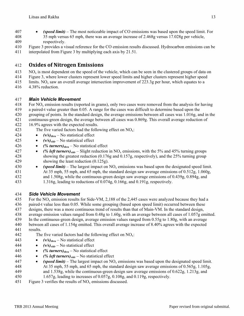
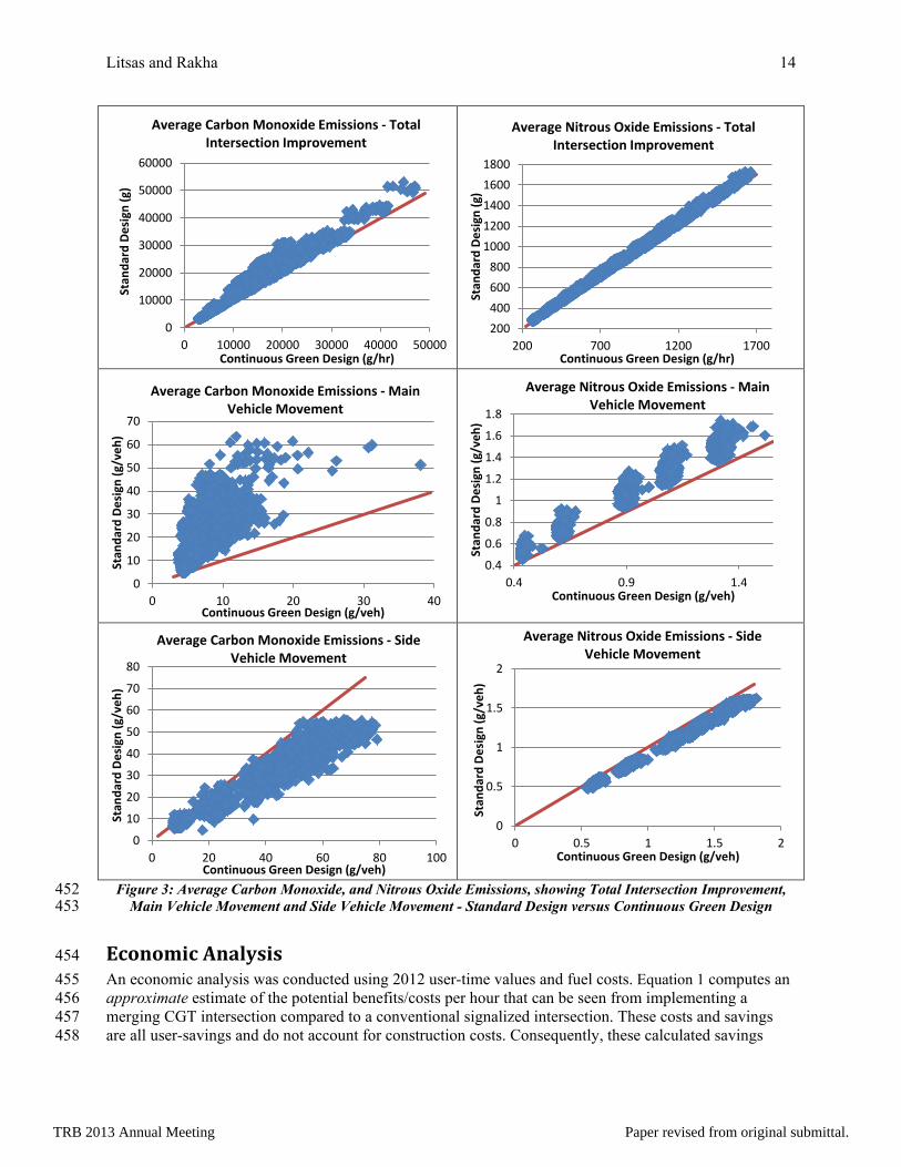
Carbon Monoxide/Hydrocarbon Emissions 362 Carbon monoxide (CO) emissions present an almost proportional correlation with hydrocarbon (HC) 363 emissions. On average, CO emissions are 21.51 more concentrated than the hydrocarbon emissions, 364 ranging from 15.10 to 25.70 more concentrated. The results saw an average overall intersection 365 improvement of 18,801g of CO (701.0g HC) saved per hour, equating to a 14.44% reduction. This 366 average overall intersection improvement can be seen graphically in Figure 3. 367

Main Vehicle Movement 368 There was a significant reduction in CO emissions between designs. For the CO emission results, 16 369 cases were removed from the analysis for having a paired-t value greater than 0.05. Most of the tests 370 reported average CO emissions per vehicle in the standard design between 5g and 50g (.30g and 2.00g 371 HC), with an 18.87g CO (0.812g HC) average between all cases. Average emissions in the continuous-372 green design showed most CO cases between 4g and 17g (0.24g and 0.70g HC) emitted per vehicle, with 373 3.77g CO (0.24g HC) appearing as a minimum threshold for all events, and a 6.74g CO (0.356g HC) 374 average between all cases. This overall average CO reduction of 64.3% (56.2% HC) agrees with the 375 expected results. 376

The five varied factors had the following effect on CO emissions: 377 • (v/s)thru – A more significant reduction in emissions per vehicle was seen when lower volumes 378

were on the main-thoroughfare versus higher volumes, with an average reduction of 14.423g 379 versus 6.739g per vehicle for the 0.4 versus 0.8 cases, respectively. 380

• (v/s)side – No statistical effect. 381 • (% turners)thru – For the percentage of turners from the main-thoroughfare, the model showed 382

that the average reduction was more significant at the highest and lowest modeled turning 383 percentage (12.778g reduction for 5% turners, 14.725g reduction for 45% turners), and least 384 significant for the 25% turners (10.731g reduction). 385

• (% left turners)side – No statistical effect. 386 • (speed limit) – The most noticeable impact on CO emissions was based upon the designated 387

speed limit within the model. When the speed limit was 35 mph versus 65 mph, there a 1.460g 388 versus 23.058g reduction per vehicle, respectively, with the reduction in emissions linearly 389 following an increasing speed limit. 390

Side Vehicle Movement 391 Side-VM showed a slight increase in CO emissions between designs. Of the 2,445 different cases, only 392 1,752 had a paired-t value less than 0.05 and were considered statistically significant. Most cases in the 393 standard design were between 5g and 57g CO (0.5g and 2.5g HC), with an average of 25.50g CO (1.27 394 HC). Most of the cases in the continuous-green design were between 8g and 78g CO (0.5g and 3.3g HC), 395 with an average of 40.90g CO (1.69g HC) emitted. All cases together yielded an average increase of 396 37.7% of CO (24.8% HC) emissions between designs. 397

The five varied factors had the following effect on CO: 398 • (v/s)thru – The volume from the main-thoroughfare showed a slight rise in increased emissions for 399

higher ratios. A ratio of 0.4 versus 0.8 yielded an average overall increase of 10.402g versus 400 12.998g per vehicle, respectively. 401

• (v/s)side – Lower left-turn volumes saw slightly larger emission increases per vehicle. 402 • (% turners)thru – Differing turning percentages were a slight factor in increased average CO 403

emissions. The 5% versus 45% case yielded a 12.623g versus 9.638g average increase per 404 vehicle, respectively. 405

• (% left turners)side – Lower percentages of left-turners saw slightly larger emission increases. 406


Litsas and Rakha 13

• (speed limit) – The most noticeable impact of CO emissions was based upon the speed limit. For 407 35 mph versus 65 mph, there was an average increase of 2.468g versus 17.028g per vehicle, 408 respectively. 409

Figure 3 provides a visual reference for the CO emission results discussed. Hydrocarbon emissions can be 410 interpolated from Figure 3 by multiplying each axis by 21.51. 411

Oxides of Nitrogen Emissions 412 NOx is most dependent on the speed of the vehicle, which can be seen in the clustered groups of data on 413 Figure 3, where lower clusters represent lower speed limits and higher clusters represent higher speed 414 limits. NOx saw an overall average intersection improvement of 223.3g per hour, which equates to a 415 4.38% reduction. 416

Main Vehicle Movement 417 For NOx emission results (reported in grams), only two cases were removed from the analysis for having 418 a paired-t value greater than 0.05. A range for the cases was difficult to determine based upon the 419 grouping of points. In the standard design, the average emissions between all cases was 1.016g, and in the 420 continuous-green design, the average between all cases was 0.869g. This overall average reduction of 421 16.9% agrees with the expected results. 422

The five varied factors had the following effect on NOx: 423 • (v/s)thru – No statistical effect 424 • (v/s)side – No statistical effect 425 • (% turners)thru – No statistical effect 426 • (% left turners)side – Slight reduction in NOx emissions, with the 5% and 45% turning groups 427

showing the greatest reduction (0.176g and 0.157g, respectively), and the 25% turning group 428 showing the least reduction (0.125g). 429

• (speed limit) – The largest impact on NOx emissions was based upon the designated speed limit. 430 At 35 mph, 55 mph, and 65 mph, the standard design saw average emissions of 0.512g, 1.060g, 431 and 1.508g, while the continuous-green design saw average emissions of 0.439g, 0.894g, and 432 1.316g, leading to reductions of 0.074g, 0.166g, and 0.191g, respectively. 433

Side Vehicle Movement 434 For the NOx emission results for Side-VM, 2,188 of the 2,445 cases were analyzed because they had a 435 paired-t value less than 0.05. While some grouping (based upon speed limit) occurred between these 436 designs, there was a more continuous trend of results than that of Main-VM. In the standard design, 437 average emission values ranged from 0.48g to 1.60g, with an average between all cases of 1.057g emitted. 438 In the continuous-green design, average emission values ranged from 0.55g to 1.80g, with an average 439 between all cases of 1.154g emitted. This overall average increase of 8.40% agrees with the expected 440 results. 441

The five varied factors had the following effect on NOx: 442 • (v/s)thru – No statistical effect 443 • (v/s)side – No statistical effect 444 • (% turners)thru – No statistical effect 445 • (% left turners)side – No statistical effect 446 • (speed limit) – The largest impact on NOx emissions was based upon the designated speed limit. 447

At 35 mph, 55 mph, and 65 mph, the standard design saw average emissions of 0.565g, 1.105g, 448 and 1.538g, while the continuous-green design saw average emissions of 0.622g, 1.213g, and 449 1.657g, leading to increases of 0.057g, 0.108g, and 0.119g, respectively. 450

Figure 3 verifies the results of NOx emissions discussed. 451


Litsas and Rakha 14

Figure 3: Average Carbon Monoxide, and Nitrous Oxide Emissions, showing Total Intersection Improvement, 452 Main Vehicle Movement and Side Vehicle Movement - Standard Design versus Continuous Green Design 453

Economic Analysis 454 An economic analysis was conducted using 2012 user-time values and fuel costs. Equation 1 computes an 455 approximate estimate of the potential benefits/costs per hour that can be seen from implementing a 456 merging CGT intersection compared to a conventional signalized intersection. These costs and savings 457 are all user-savings and do not account for construction costs. Consequently, these calculated savings 458

0

10000

20000

30000

40000

50000

60000

0 10000 20000 30000 40000 50000

Stan

dard

Des

ign

(g)

Continuous Green Design (g/hr)

Average Carbon Monoxide Emissions - Total Intersection Improvement

200400600800

10001200140016001800

200 700 1200 1700

Stan

dard

Des

ign

(g)

Continuous Green Design (g/hr)

Average Nitrous Oxide Emissions - Total Intersection Improvement

0

10

20

30

40

50

60

70

0 10 20 30 40

Stan

dard

Des

ign

(g/v

eh)

Continuous Green Design (g/veh)

Average Carbon Monoxide Emissions - Main Vehicle Movement

0.4

0.6

0.8

1

1.2

1.4

1.6

1.8

0.4 0.9 1.4

Stan

dard

Des

ign

(g/v

eh)


Average Nitrous Oxide Emissions - Main Vehicle Movement

0

10

20

30

40

50

60

70

80

0 20 40 60 80 100

Stan

dard

Des

ign

(g/v

eh)


Average Carbon Monoxide Emissions - Side Vehicle Movement

0

0.5

1

1.5

2

0 0.5 1 1.5 2

Stan

dard

Des

ign

(g/v

eh)


Average Nitrous Oxide Emissions - Side Vehicle Movement


Litsas and Rakha 15

should be coupled with a construction estimate in order to evaluate the feasibility of a CGT intersection. 459 Construction costs were not analyzed as part of this research due to the high variability of costs based 460 upon current conditions, leaving a large potential range of construction costs. X1, X2, X3, and X4, are 461 average weighting factors determined from the modeled run conditions. These factors, found in Table 1, 462 vary as a function of the approach speed limit of the main-thoroughfare, and total volumes on the main-463 thoroughfare and side-street. V1 and V2 are inserted as total volumes, which can be found by taking the 464 volume of the main-thoroughfare or side-street and reducing accordingly for the percentage of turning 465 traffic. X1 and X2 are based upon V1; X3 and X4 are based upon V2. To utilize this equation for a 24-hour 466 period, calculate each hour independently and sum the savings/costs. 467 468 Equation 1: Cost/Savings (per hr) = {[(𝑿𝟏 × 𝑪𝟏) + (𝑿𝟐 × 𝑪𝟐)] × 𝑽𝟏} − {[(𝑿𝟑 × 𝑪𝟏) + (𝑿𝟒 × 𝑪𝟐)] × 𝑽𝟐} 469

where: X1, X2, X3, X4 = factors found in Table 1 470 V1 = volume of main vehicle movement, per hour 471 V2 = volume of side vehicle movement, per hour 472 C1 = cost of user time ($/hr) 473 C2 = cost of unleaded gasoline ($/gallon) 474 475

Table 1: Factors to Solve Equation 1 476 V1 X1 X2 V2 X3 X4

792 to 1278 0.00265 0.00455 18 to 103 0.00076 0.002401279 to 1764 0.00230 0.00429 104 to 188 0.00095 0.002841765 to 2250 0.00211 0.00350 189 to 274 0.00119 0.003362251 to 2736 0.00247 0.00367 275 to 360 0.00123 0.00356





35 mph cases:

45 mph cases:

55 mph cases:

60 mph cases:

65 mph cases:

477

Overall Economic Analysis 478 This initial analysis uses all cases as an average for computing the cost/savings of implementing a CGT 479 design. The results demonstrate that significant savings can be achieved for the Main-VM with relatively 480 low additional costs for Side-VM vehicles. The analysis considered a user cost of $32/car/hour [13] and 481


Litsas and Rakha 16

fuel costs of $3.39/gallon [14]. In computing the average cost/savings for all runs, the delay and fuel 482 consumption for both the Main-VM and Side-VM were only considered for statistically significant cases 483 (i.e. probability of 0.05 or less). Only 1,485 of the 2,445 tests met this condition. It should be noted that 484 the averages for all 2,445 cases were very similar to the average over 1,485 cases. 485

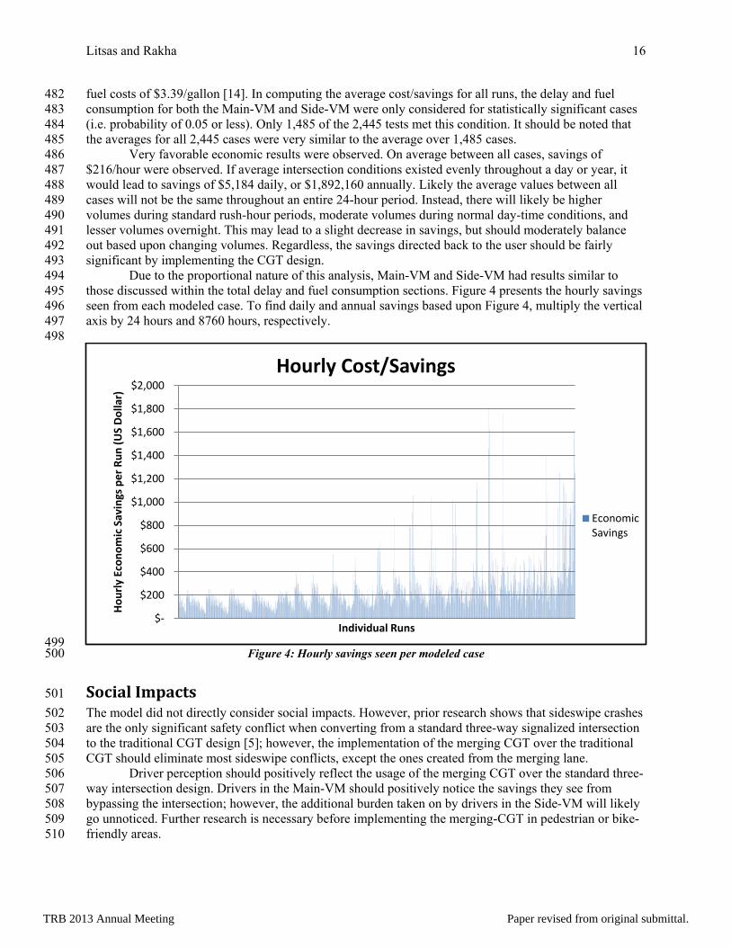
Very favorable economic results were observed. On average between all cases, savings of 486 $216/hour were observed. If average intersection conditions existed evenly throughout a day or year, it 487 would lead to savings of $5,184 daily, or $1,892,160 annually. Likely the average values between all 488 cases will not be the same throughout an entire 24-hour period. Instead, there will likely be higher 489 volumes during standard rush-hour periods, moderate volumes during normal day-time conditions, and 490 lesser volumes overnight. This may lead to a slight decrease in savings, but should moderately balance 491 out based upon changing volumes. Regardless, the savings directed back to the user should be fairly 492 significant by implementing the CGT design. 493

Due to the proportional nature of this analysis, Main-VM and Side-VM had results similar to 494 those discussed within the total delay and fuel consumption sections. Figure 4 presents the hourly savings 495 seen from each modeled case. To find daily and annual savings based upon Figure 4, multiply the vertical 496 axis by 24 hours and 8760 hours, respectively. 497

498

499 Figure 4: Hourly savings seen per modeled case 500

Social Impacts 501 The model did not directly consider social impacts. However, prior research shows that sideswipe crashes 502 are the only significant safety conflict when converting from a standard three-way signalized intersection 503 to the traditional CGT design [5]; however, the implementation of the merging CGT over the traditional 504 CGT should eliminate most sideswipe conflicts, except the ones created from the merging lane. 505

Driver perception should positively reflect the usage of the merging CGT over the standard three-506 way intersection design. Drivers in the Main-VM should positively notice the savings they see from 507 bypassing the intersection; however, the additional burden taken on by drivers in the Side-VM will likely 508 go unnoticed. Further research is necessary before implementing the merging-CGT in pedestrian or bike-509 friendly areas. 510

$-

$200

$400

$600

$800

$1,000

$1,200

$1,400

$1,600

$1,800

$2,000

Hour

ly E

cono

mic

Sav

ings

per

Run

(US

Dolla

r)

Individual Runs

Hourly Cost/Savings

EconomicSavings


Litsas and Rakha 17

Conclusions 511

A comparison of the merging CGT to the standard signalized intersection shows very positive results. The 512 merging CGT outperforms the standard design in every modeled case for the six analyzed factors, and 513 thus is a more optimal design for three-way “at grade” intersections. Table 2 summarizes the average 514 results and percent reduction/increase seen by Main-VM and Side-VM when implementing a merging 515 CGT. The total volumes from the main-thoroughfare being higher than the side-street showed a total 516 intersection reduction in every situation. Additionally, low reduction/increase percentages can be 517 attributed to the 4 km modeling distance, where shorter modeling distances would have shown larger 518 reductions/increases per vehicle. 519 520

Table 2: Summary Results 521

Category:

Traditional Design

Average

Continuous Green Design

Average% Reduction

Traditional Design

Average

Continuous Green Design

Average% Increase

Total Reduction

% Reduction

Total Delay (s) 11.41 0.68 94.0% 38.9 42.0 7.4% 18,242 10.29%Fuel Usage (l) 0.367 0.331 9.8% 0.392 0.412 4.9% 54.1 2.78%Hydrocarbon (g) 0.812 0.356 56.2% 1.27 1.69 24.8% 701.0 12.47%Carbon Monoxide (g) 18.87 6.74 64.3% 25.50 40.90 37.7% 18,801 14.44%Nitrous Oxide (g) 1.016 0.869 16.9% 1.057 1.154 8.4% 223.3 4.38%Carbon Dioxide (g) 828.09 762.83 7.9% 872.69 913.17 4.4% 99,376 2.29%

Main Vehicle Movement (per veh) Side Vehicle Movement (per veh) Total Intersection Improvement (per hr):

522 523

When transitioning an intersection to the continuous-green design, the total delay and fuel usage 524 for Main-VM vehicles is significantly reduced with very little additional delay or fuel usage for Side-VM 525 vehicles. 526

Environmentally, the merging CGT design outperforms the standard signalized intersection for all 527 four modeled emissions. For Main-VM, significant reductions were observed for HC, CO, NOx, and CO2 528 emissions. For Side-VM, not as significant average increases were seen in HC, CO, NOx, and CO2 529 emissions. Due to the typically much lower volumes on the side-street versus the main-thoroughfare, any 530 increases from Side-VM will easily be outweighed by the much higher volume of traffic on the main 531 street. 532

Economically, the merging CGT design is better than the standard signalized intersection. Based 533 upon current economic conditions, merging CGT designs will result in savings in the range of $224/hour 534 for Main-VM vehicles, with more significant savings seen during periods of high-traffic volumes. 535 Furthermore, minor additional costs ($8.05/hour on average) are incurred on Side-VM vehicles. This 536 design improvement can see average savings at $5,184 daily, or $1,892,160 annually. Furthermore, 537 socially this type of intersection control should increase driver satisfaction in Main-VM through delay 538 reduction, with minimal additional costs associated with the Side-VM. 539

The most significant factor that affects the benefits of a merging CGT intersection is the approach 540 speed limit. Specifically, higher speed limits lead to more significant improvements in the intersection 541 performance relative to a standard traffic signal controlled intersection. Additionally, Side-VM showed 542 that in all cases except for total delay, the increased burden taken on by the vehicles is most dependent on 543 the speed limit of the main-thoroughfare. However, because the rate of reduction for Main-VM increased 544 at a rate faster than the rate of increase for Side-VM, a higher speed limit continually shows higher 545 savings in all six analyzed factors. 546

An increasing volume on the main-thoroughfare showed increasing levels of reduction in total 547 delay and fuel consumption for Main-VM vehicles. Yet, lower volumes on the main-thoroughfare saw 548


Litsas and Rakha 18

more significant reductions in terms of HC and CO emissions, with no significant impact on NOx or CO2 549 emissions. For Side-VM vehicles, only fuel consumption and CO2 emissions were affected by the volume 550 of the main-thoroughfare, showing an increase with higher speeds. Total delay, HC, CO, and NOx 551 emissions had very little impact on Side-VM vehicles for (v/s)thru. 552

The percent of turners from the main-thoroughfare onto the side-street had an interesting effect on 553 five of the six analyzed categories in Main-VM, excluding total delay. For these five categories, the 554 lowest and highest modeled turning percentages showed the highest reductions, while the middle modeled 555 turning percentage showed the lowest reduction. This did not correlate the same with Side-VM, as fuel 556 consumption, HC, CO, and CO2 emissions saw very small increases with lower turning percentages, yet 557 total delay and NOx emissions saw no impact based upon (% turners)thru. 558

In general, the volume of the side-street and the percent of left turners on the side-street had very 559 little effect on the six analyzed factors for both Main-VM and Side-VM. 560

In conclusion, the merging CGT design is favorable over the standard signalized design in every 561 modeled situation. It is most optimal to implement this design at intersections with higher speeds along 562 the main-thoroughfare. Additionally, cases with higher volumes along the main-thoroughfare and lower 563 volumes on the side-street are most favorable as it will lead to more significant benefits. The 564 volume/saturation (v/s) ratio of the main-thoroughfare showed greater intersection improvement when 565 utilized for higher v/s conditions. The v/s ratio and percent of turners from the side-street should not 566 affect the decision to implement a merging CGT design. The cost/benefit ratio based upon roadway 567 volume should greatly affect the decision to install the merging CGT, determinant upon construction costs 568 necessary to retrofit from the standard intersection control. 569

This paper could serve as a reference for examining the environmental benefits of other 570 innovative intersection designs. 571 572


Litsas and Rakha 19

Works Cited 573

574 [1] J. Boone and J. Hummer, "Unconventional Design and Operation Stratagies for Over-Saturated

Major Suburban Arterials," Center for Transportation Engineering Studies, Department of Civil Engineering, North Carolina State University, Raleigh, 1995.

[2] E. Jarem, "Safety and Operational Characteristics of Continuous Green Through Lanes at Signalized Intersections in Florida," Faller Davis & Associates, Maitland, 2004.

[3] J. Reid, "Unconventional Arterial Intersection Design, Management, and Operation Strategies," Parsons Brinckerhoff, New York, 2004.

[4] E. Rice and Z. Znamenacek, "Intersection Safety Case Study - Continuous Green T-Intersections," Federal Highway Administration, 2009.

[5] T. Sando, D. Chimba, V. Kwigzile and H. Walker, "Safety Analysis of Continuous Green Through Lane Intersections," Transportation Research Board, Washington, 2010.

[6] S. Park and H. Rakha, "Continuous Flow Intersections: A Safety and Environmental Perspective," in 13th International IEEE: Annual Conference on Intelligent Transportation Systems, Madeira Island, Portugal, 2010.

[7] M. El Esawey and T. Sayed, "Analysis of Unconventional Arterial Intersection Designs (UAIDs): State-of-the-Art Methodologies and Future Research Directions," Transportmetrica, vol. doi: 10.1080/18128602.2012.672344, pp. 1-36, 2012.

[8] Texas Department of Transportation, Roadway Design Manual, Chapter 3, Figure 3-36, Design Devision, 2010.

[9] H. Rakha, I. El-Shawarby, S. Park and M. Arafeh, "Modeling Framework for the Evaluation of Alternative Truck Lane Management Strategies," Intelligent Transportation Systems (ITSC), pp. 1025-1032, 2010.

[10] F. Dion, H. Rakha and Y.-S. Kang, "Comparison of delay estimates at under-saturated and over-saturated pre-timed signalized intersections," Transportation Research Part B-Methodological, vol. 38, pp. 99-122, 2004.

[11] F. Webster, "Traffic Signal Settings," in Road Research Technical Paper No. 39, London, Great Britian Road Research Laboratory, 1958.

[12] Transportation Research Board, Highway Capacity Manual, 4th ed., Washington, 2000. [13] V. Perk, J. DeSalvo, T. Rodrigues, N. Verzosa and S. Bovino, "Improving Value of Travel Time

Savings Estimation for More Effective Transportation Project Evaluation," Center for Urban Transportation Research, University of South Florida, Tampa, 2011.

[14] AAA, "Daily Fuel Gauge Report - National Average Prices," 13 February 2012. [Online]. Available: http://fuelgaugereport.aaa.com/. [Accessed 13 February 2012].

575 576 577 578


evaluation of continuous green t-intersections on …docs.trb.org/prp/13-0591.pdf1 evaluation of...

Documents