evaluation of analytical methods for measuring the

Journal Of Oil, Gas and Petrochemical Technology 7(1): 59-74, Autumn 2020

RESEARCH PAPER

Evaluation of Analytical Methods for Measuring the Molecular Diffusion Coefficient in Gas-Oil Systems by the Pressure Decay MethodFereshte Zareie1 , Reza Azin *2, Shahryar Osfouri1, Hossein Rahideh1

1. Department of Chemical Engineering, Faculty of Oil, Gas and Petrochemical Engineering, Persian GulfUniversity, Bushehr, Iran2. Department of Petroleum Engineering, Faculty of Oil, Gas and Petrochemical Engineering, Persian GulfUniversity, Bushehr, Iran

* Corresponding Author Email: [email protected]

ARTICLE INFO

Article History:Received 18 April 2020Accepted 21 Augest 2020 Published 01 July 2020

Keywords:Diffusion coefficient Pressure decay method Gas injectionGas-Oil systemsAnalytical method

ABSTRACT

How to cite this article: Zareie F., Azin R., Osfouri S., Rahideh H. Evaluation of Analytical Methods for Measuring the Molecular Diffusion Coefficient in Gas-Oil Systems by the Pressure Decay Method. Journal of Oil, Gas and Petrochemical Technology, 2020, 7(1): 59-74. DOI: 10.22034/jogpt.2020.119830

Gas is injected into reservoirs for pressure maintenance, enhanced oil recovery and greenhouse gas storage. The molecular diffusion coefficient is one of the most important mechanisms in describing the mass transfer of gas during injection. The molecular diffusion coefficient is determined using indirect methods like pressure decay method associated with appropriate models and analyzing the experimental results. In this study, analytical methods for analyzing the experimental data from the pressure decay method were evaluated. For this purpose, three analytical solution methods of diffusivity equation were introduced using equilibrium, quasi-equilibrium and non-equilibrium boundary conditions at the interface of two phases in contact with the diffusion cell. Then, the models were applied for determining diffusivity in different fluid systems of heavy and light oil. The evaluation of the proposed models was based on the difference between the production pressure by these models and the experimental pressure. The results showed that for heavy oil systems, the boundary conditions on the surface is dependent on the type of the injection gas and the experimental conditions. Equilibrium boundary conditions are used for light oil systems because of their lower viscosity and continuity at the interface of two phases.

IntroductionGas injection is widely used in enhanced oil

recovery processes. The molecular diffusion coefficient, even a very low one, plays an essential role in the gas injection process. Therefore, accurate estimation of the molecular diffusion coefficient is necessary for designing processes related to the enhanced oil recovery from reservoirs [1]. More than 60% of the world's oil resources are in carbonate reservoirs, most of which are natural fractures. One of the important mechanisms of production in fracture

reservoirs under gas injection is the molecular diffusion that can increase oil recovery [2-4]. Kazemi et al. studied carbon dioxide injection and molecular diffusion in fracture reservoirs. The results showed that the combined effect of molecular diffusion and gravity is very important in the simulation of fracture reservoirs[5]. The diffusion occurs as a result of the random movement and collision of the molecules and originates from the difference of chemical potential due to the concentration difference of the components in a multi-component system.

This work is licensed under the Creative Commons Attribution 4.0 International License.To view a copy of this license, visit http://creativecommons.org/licenses/by/4.0/.

60

R.Azin et al. / Evaluation of Analytical Methods for Measuring the Molecular Diffusion Coefficient

The diffusion coefficient is a physical parameter that represents the quality of the diffusion process and is measured with both direct and indirect methods. One of the most important and widely-used methods of measurement of the diffusion coefficient in gas-liquid systems is the pressure decay method, which was first introduced by Riazi [6]. Unlike other methods, the pressure decay method is very easy and accurate [7]. In this method, the gas pressure decreases as the gas phase molecules diffuse into the liquid phase in a high-pressure cell. The diffusion process continues until the liquid phase is saturated with the gas phase [8]. Different mathematical models have been proposed to determine the diffusion coefficient from the pressure-time laboratory data and all the proposed models have been derived from applying the continuum equation and different boundary conditions. Table 1 shows the research presented in the pressure decay method based on different boundary conditions.

For the first time, Riazi (1996) used the pressure decay method to measure the diffusion coefficient. He measured the methane diffusion coefficient in normal pentane by measuring the pressure decay rate and presented a semi-

analytical model considering quasi-equilibrium boundary conditions in the interface and the effect of liquid swelling over time[6]. Zhang et al. introduced the diffusion coefficient as a function of equilibrium pressure by simplifying the problem and ignoring the fluid phase volume changes. They assumed equilibrium on the surface by combining the analytical and graphical methods [9]. Uperti et al. considered the volumetric expansion effect and thus considered the time-dependent equilibrium concentration, which is physically more accurate than the model proposed by Zhang et al. [10] Tharanivasan et al. calculated the diffusion coefficient at Dirichlet, Newman and Robin boundary conditions for the carbon dioxide and methane heavy oil systems. They reported that the diffusion coefficient is sensitive to the boundary conditions between the two phases, and, depending on the type of fluid, different boundary conditions must be used for modeling[8, 11]. Sheikha et al. presented new boundary conditions using the integration of a diffusion equation and a mass balance equation and calculated the diffusion coefficient using a graphical method [12, 13]. Civan and Rasmussen calculated the diffusion coefficient for the

Table1: Classification of boundary conditions at the gas-liquid interface

ReferenceBoundary conditionsDesired systemAuthors[6]Quasi-equilibriumCH4 - Normal PentaneRiazi (1996)[9]EquilibriumCO2 /CH4 – Heavy OilZhang et al. (2000)

[10, 20]Quasi-equilibriumCO2 /CH4 - BitumenUpreti et al. (2000-2002)[8, 11]Equilibrium Quasi-equilibrium

Non-equilibriumCO2 /CH4 – Heavy OilTharanivasan et al.

(2004-2006)

[12, 13]Quasi-equilibriumCO2 /CH4 - BitumenSheikha et al. (2004-2006)

[21]EquilibriumCO2 - Carbonated/OilRiazi et al. (2011)

[1, 17, 22]Non-equilibriumCO2 /CH4 - BitumenEtminan et al. (2013)[23]Quasi-equilibriumCO2 – AquiferAzin et al. (2013)[24]Quasi-equilibriumCO2 – AquiferRaad et al. (2015)[25]EquilibriumCO2 – AquiferShi et al. (2018)[26]Non-equilibriumCO2 – Isooctane/HexanolNategh et al. (2018)

[27-29]EquilibriumCO2 – OilLi et al. (2016-2018)[30]EquilibriumCO2 /CH4 - BitumenRahide & Azin (2018)[31]EquilibriumCO2 – OilGao et al. (2019)


61Journal Of Oil, Gas and Petrochemical Technology 7(1): 59-74, Autumn 2020


laboratory data of Zhang and Sheikha et al. considering the surface resistance at the two-phase boundary [14-16]. By introducing a mass transfer factor, Etminan et al. argued that there is a discontinuity at the interface due to the resistance between the two phases, and this discontinuity on the surface is proportional to the mass diffusion flux [17]. Ohata et al. determined the diffusion coefficient of gas in heavy oil and gas condensate with the pressure decay method in the diffusion cell. The results showed a 10-fold increase in the condensate diffusion coefficient, compared to heavy oil. They also examined the recovery of oil in the presence and absence of molecular diffusion and observed a 10% increase in the presence of the molecular diffusion [18] . Francisco et al. investigated the diffusivity and solubility of methane and carbon dioxide in normal decane, hexadecane and bitumen over a wide range of temperatures by the pressure decay method in equilibrium boundary conditions [19]. Francisco et al. investigated the diffusivity and solubility of methane and carbon dioxide in normal decane, hexadecane and bitumen over a wide range of temperatures with the pressure decay method in equilibrium boundary conditions and reported the diffusion coefficient and hennery’s constant for the listed systems, using a graphical method.

In this study, different models of analyzing

laboratory data with the pressure decay method were investigated. Then, the assumptions of each of these models were presented along with their analytical solutions. In order to evaluate these models, the diffusion coefficients and pressures of CO2 and CH4 gases in heavy oil, dodecane and hexadecane were calculated and then compared using the different boundary conditions and analytical solutions. Finally, the most suitable model for the light and heavy oil systems was determined. The most important point in the pressure decay method is to choose the boundary condition and the appropriate model with the problem conditions. Using the results of the present study, it is possible to select the appropriate model according to the physics of the problem and report the diffusion coefficient with the least amount of error without performing high-volume calculations.

2-Pressure Decay MethodThe system of pressure decay method

for measuring the diffusion coefficient of the gases in liquids is shown in Fig. 1. In this method, gas is deposited on a volume of fluid in a diffusion cell with uniform temperature and a constant volume. The Non-volatile liquid phase is in contact with the gas phase, and, as a result, the gas gradually diffuses into the fluid until the fluid is saturated. As a result of

Figure 1. Schematic of pressure decay method [23]

62


the dissolution of the dissolved gas, the gas pressure decreases. The process of gas pressure changes is recorded. Based on the gas pressure changes in the chamber and its relation to the gas concentration changes in the liquid, the diffusion coefficient is calculated.

In order, the experimental data of Etminan et al. [22] was used to investigate heavy oil systems, and the experimental data of Francisco et al. [19] was used to investigate the light oil systems. Table 2 shows the conditions of the experiments.

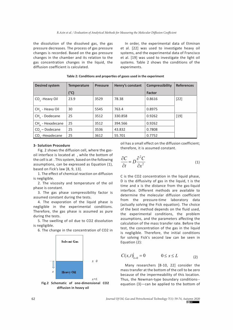
3- Solution ProcedureFig. 2 shows the diffusion cell, where the gas-

oil interface is located at , while the bottom of the cell is at . This system, based on the following assumptions, can be expressed as Equation (1), based on Fick’s law [8, 9, 13].

1. The effect of chemical reaction on diffusion is negligible.

2. The viscosity and temperature of the oil phase is constant.

3. The gas phase compressibility factor is assumed constant during the tests.

4. The evaporation of the liquid phase is negligible in the experimental conditions. Therefore, the gas phase is assumed as pure during the tests.

5. The swelling of oil due to CO2 dissolution is negligible.

6. The change in the concentration of CO2 in

oil has a small effect on the diffusion coefficient; therefore, it is assumed constant.

2

2

xCD

tC

∂∂

=∂∂

(1)

C is the CO2 concentration in the liquid phase, D is the diffusivity of gas in the liquid, t is the time and x is the distance from the gas-liquid interface. Different methods are available to determine the molecular diffusion coefficient from the pressure-time laboratory data (actually solving the Fick equation). The choice of the best method depends on the fluid used, the experimental conditions, the problem assumptions, and the parameters affecting the calculation of the mass transfer rate. Before the test, the concentration of the gas in the liquid is negligible. Therefore, the initial conditions for solving Fick's second law can be seen in Equation (2):

0),(0=

=ttxC Lx ≤≤0 (2)

Many researchers [8-10, 22] consider the mass transfer at the bottom of the cell to be zero because of the impermeability of this location. Thus, the Newman-type boundary conditions--equation (3)—can be applied to the bottom of

Table 2: Conditions and properties of gases used in the experiment

ReferencesCompressibility

Factor

Henry’s constantPressureTemperature

(°C)

Desired system

[22]0.861678.38352923.9CO2 -Heavy Oil

0.8975763.4554530CH4 - Heavy Oil

[19]0.9262330.858351225CH4 - Dodecane

0.9262394.566351225CH4 - Hexadecane0.780843.832353625CO2 – Dodecane0.775255.701361225CO2 -Hexadecane

Fig.2 Schematic of one-dimensional CO2 diffusion in heavy oil


63


the diffusion cell:

0=∂∂

=LxxC

0>t (3)

The boundary conditions at the interface largely depend on the type of fluid. In the following, the boundary conditions at the interface, the solution of diffusion equation and the calculation of the diffusion coefficient for the two systems including gas-heavy oil and gas-light oil will be compared.

3-1- Zhang's analytical solution (assuming equilibrium boundary conditions at the interface)

Assuming that at all times the concentration at the interface is equal to the concentration at the equilibrium pressure (i.e., the interface

conditions are equal to the equilibrium conditions), the Dirichlet boundary conditions (Equation 4) for the diffusion process can be applied:

)(),(0 eqeqx

PCtxC ==

0>t (4)

Equation (5) is obtained by the analytical solution of Equation 1 based on the initial and boundary conditions given in Equations 2-4 (Appendix A)[9, 32].

Using the mass balance and Fick's first law (Equation 6), it is possible to relate the system pressure to the diffusion concentration (given in Appendix A) and to obtain pressure changes in the gas phase (Equation 7) from the concentration changes in the liquid phase.

(5)

(6)

(7)

By plotting the experimental data (Logarithm of the difference of instantaneous pressure and equilibrium pressure over time) based on Equation (7), a straight-line fit can be obtained. From the slope and the intercept of the resulting line, the diffusion coefficient (Equation (8)) and the solubility of gas in oil can be calculated[9].

2

2

4LDslope π

−= (8)

3-2- Sheikha's analytical solution (assuming pseudo-equilibrium boundary conditions at the interface)

The most important assumption that Sheikha et al. used in their method is the assumption of thermodynamic equilibrium at the interface of gas and bitumen. Also, earlier, before the closed

boundary at the cell bottom affects the rate of the mass transfer between the gas and the bitumen, an infinite-acting boundary condition can be assumed. According to the assumptions of the problem using Fick’s second law and the assumption of an infinite boundary for the system, the concentration is considered to be zero, and Fick’s second law is solved by the two boundary conditions according to equation (9) and (10) [13].

(9)

The boundary conditions at the interface is obtained by taking into account of two assumptions: the assumption of equilibrium at

0=x

4 ( ) 2 2( 1) (2 1) (2 1 )( , ) cos exp 22 1 2 40

C P n n z n Dsat eqC x t C tsat n L Ln

π ππ

∞ − + + = − −∑ + =

0

( )

g x

dP t ZRT dCDdt h dx =

= −

2

2 2

8 ( )ln ( ) ln

4sat eq

eq

ZRTC P DP t P th L

ππ

− = −

dC V dPdx ZRTDA dt

=


64


the interface and the assumption that the mass of the diffused gas in the liquid is equal to the difference between the initial and final mass of the gas, according to the principle of mass conservation. During early times, before the closed boundary at the cell bottom affects the rate of mass transfer between the gas and the oil, an infinite-acting boundary condition can be assumed[12]:

0=C ∞→x (10)

Sheikha et al. solved Equation (1) with boundary conditions—Equations (9) & (10)—and the Laplace method and expressed the gas concentration in the liquid phase in terms of a function of penetration depth and time. Using Henry's law, they also obtained the system pressure changes according to Equation (11) [32]:

=

hhi LMK

tZRTDerfcLMK

tZRTDPtP2

exp)(

(11)

Then, by ignoring the exponential term and

differentiating with respect to t , the following equation will be formed:

LMKZRTD

td

PtPerfcd

h

i =

−

)(

)(1

(12)

According to Equation (12), by plotting

−

iPtPerfcd )(1

over )( td , a straight-line fit can be obtained. The diffusion coefficient can be calculated from the slope of the resulting line with Equation (13).

2)(ZRT

LMKbD h=

(13)

b is the slope of the strain line; L is the height of gas zone in the pressure cell, M is the molar mass of gas and Kh is Henry’s constant. In Sheikha's analytical solution, Henry's law is used for the boundary conditions of the interface, and, since Henry's law is based on the instantaneous

equilibrium, the resistance between the two phases is considered negligible in this method.

3-3- Etminan's analytical solution (assuming a non-equilibrium boundary condition at the interface)

In this analytical solution, the effect of resistance against mass diffusion at the interface is considered, which means the gas concentration on the contact surface is discontinuous. Etminan et al. [17] applied Equation (14) to the boundary conditions between the two phases by applying discontinuities.

)),0()(( int0

txCtCkx

CD gg

x

g =−=∂

∂− −

= (14)

They expressed the equilibrium concentration by means of Henry’s law and solved the equation by Laplace's method. As a result, they obtained the gas cap pressure according to Equation (15) in the Laplace form and finally applied the Stehfest algorithm to find the inverse transform.

ZRTDKMh

M hwg=

ZRTK

KMhN hwg=

(15)

4. Results and Analysis4-1- Diffusion coefficient values in heavy oil-gas systems

Figure 3 shows the pressure reduction over time during the dissolution of carbon dioxide and methane in heavy oil according to Etminan et al. [22].

As shown in Figure 3, the minimum time required to achieve carbon dioxide equilibrium is less than the one required for methane. Figure 3 also shows a further reduction in pressure for the carbon dioxide system. The change in pressure in the carbon dioxide system before equilibrium is 726 kPa, which is about 20% of the initial pressure, while, in the methane system,

( ) ( )

2 2

2

1 ( )

( )

1 ( 1 )

S SL LD D

i

S LD

D S SMp e eK D D

P SS SMS NS e MS NSD D

− −

−

+ − − =

+ + + − +


65


it is about 6.5% of the initial pressure. This indicates the high solubility of carbon dioxide gas and its high capacity for use in gas injection into the reservoirs. Table 3 shows the pressure changes for different systems over 5 days.

Table 4 shows the diffusion coefficient

values determined for the dissolution of carbon dioxide and methane in heavy oil based on the experimental data of Etminan et al. with the analytical solutions mentioned in the previous section. In the case of the CO2-heavy oil system, as can be seen, the diffusion coefficient values calculated with the non-equilibrium boundary

Figure 3. Pressure decay graph[22]

Table 3: Gas pressure changes over 5 days by pressure decay method

ReferenceGas pressure

changes

PressureTemperature

(°C)

SystemResearchers

[9]11.6

1.4

3471

3510

21

21

CO2– Heavy Oil

CH4 – Heavy Oil

Zhang et al. (2000)

[11]7.2

1.05

4176

5013

23.9

23.9

CO2– Heavy Oil

CH4 – Heavy Oil

Tharanivasan et al. (2006)

[17]11.7

1.8

3529

5545

23.9

30

CO2– Heavy Oil

CH4 – Heavy Oil

Etminan et al. (2013)

condition are smaller. In the case of non-hydrocarbon solvents such as carbon dioxide, combustion gas and nitrogen, due to the strong surface resistance between the interfaces, the system comes to equilibrium late and the diffusion coefficient decreases in the non-equilibrium boundary condition[8].

In the case of the diffusion of methane, ethane and propane into hydrocarbons, the dissolution

takes place faster because the solvent and the solute have the same chemical structure[8]. According to studies [6, 9, 11], in methane-heavy oil systems, there is less resistance at the interface between the two phases, and the rate of diffusion is higher than the carbon dioxide-heavy oil system, which causes the two-phase surfaces to reach the equilibrium faster. In the case of Etminan et al.'s experimental data for


66


the methane heavy oil, the system reaches equilibrium after about a 6.5% reduction in the initial pressure. This low pressure change could suggest that, in a methane heavy oil system, the use of equilibrium boundary conditions is preferred over the non-equilibrium boundary conditions[8]. Figure 4 shows the experimental pressure measured by Etminan et al. and the computational pressure by the Zhang, Sheikha and Etminan model for the CO2 and methane systems in heavy oil. In CO2 dissolution in heavy oil at equilibrium boundary conditions, the difference between the calculated pressure and the measured pressure at the beginning of the process is more than the difference at the end of the process, i.e., near the equilibrium state of the system. Achieving equilibrium boundary conditions depends on reaching the saturation concentration, and since the interface of heavy oil- CO2 does not reach thermodynamic equilibrium fast, the difference between the measured pressure and the calculated pressure

is observed at the dissolution initial stages. As can be seen from Fig. 4a, there is a large difference between the pressure measured with Sheikha et al.’s assumptions and the experimental data. This difference is mostly related to the fourth day onwards and may indicate that the infinite-acting assumption for the heavy oil-CO2 system is incorrect and the gas concentration penetrates to the bottom of the cell [23].

The non-equilibrium boundary condition increases the time to reach equilibrium by considering the dissolution resistance in the two-phase contact surface and is able to better match the experimental data. The use of non-equilibrium boundary conditions is largely dependent on the mass transfer coefficient between the two phases. Physically when the mass transfer coefficient is large enough or the

Table 4: Diffusion coefficient values for heavy oil-gas system under different boundary conditions

System Boundary conditions Analytical Solutions Diffusion Coefficient*10-10

CO2– Heavy Oil

Equilibrium Separation of variables

1.42

Quasi-equilibrium Laplace 2.34

Non-equilibrium Laplace 1.34

CH4 – Heavy Oil

Equilibrium Separation of variables

0.813

Quasi-equilibrium Laplace 2.29Non-equilibrium Laplace 0.766

Fig.4 Comparison of laboratory pressure decay and measured pressure decay for the analytical models of Zhang, Sheikha, and Etminan A: CO2-heavy oil system B: CH4-heavy oil system.


67


interfacial resistance between the two phases is low enough, the non-equilibrium boundary condition approaches the equilibrium boundary condition. The value of varies from zero to infinity. is equivalent to the absence of surface resistance between the two phases and the infinite mass transfer or equilibrium boundary condition. However, if , the analytical solution of the diffusion equation cannot be used. may occur in two cases. The first occurs when the gas is insoluble in liquid, which is not the case for the miscible gas injection systems. The latter occurs when the diffusion coefficient is infinite or the liquid column length is too small[8]. Therefore, assumptions such as the length of the gas and liquid column, the initial pressure of the gas, and the type of system desired determine the boundary conditions and the analytical method used in the pressure decay method [8]. In the methane-heavy oil system, as shown in Figure 4b, the error between the pressure measured with the equilibrium boundary condition and the experimental pressure is not significantly different from the error between the pressure measured with the non-equilibrium boundary condition and the experimental pressure. However, there is a big difference between the analytical solution to Sheikh's assumptions and the experimental data.

4-2- Diffusion coefficient values in light oil-gas systems

Since the gas injection is less used for the light oil extraction, unlike heavy oil, there are fewer data on the pressure decay method for the light oil compounds in the literature. Fig. 5 shows the time-dependent pressure decay process during carbon dioxide and methane dissolution in dodecane and hexadecane according to the laboratory data of Francisco et al. [19].

As seen in Figure 5, most of the pressure changes belong to the dissolution of carbon dioxide in dodecane. This is due to the fact that carbon dioxide is more soluble than methane, especially in dodecane, which is lighter than the hexadecane. Table 5 shows the diffusion coefficient values calculated for the carbon dioxide and methane dissolution in dodecane

and hexadecane according to the experimental data of Francisco et al. A comparison of Table 4 and Table 5 shows that the diffusion coefficient in light oil compounds is almost 100 times higher than the heavy oil. This implies that there can be a relationship between the diffusion coefficient and the oil property, i.e. the higher the density and viscosity on the oil, the smaller the diffusion coefficient.

Table 5 shows that, under the same temperature (25 °C) and pressure conditions, the CO2 diffusion coefficient in light oil is ten times as much as that of the CH4, and the diffusivity coefficient of the two gases in dodecane is higher than that of hexadecane. Figure 6 shows the laboratory pressure measured by Francisco et al. and the pressure calculated through the Zhang and Sheikha analytical solutions. Light oil flows easily and contains more volatile components, while heavy oil is highly viscous to nearly tar-like and show a higher density. Due to the low viscosity of the light composites, compared to heavy oil, it can be said that the equilibrium boundary condition has good agreement with the experimental data. Whereas the pseudo-

Figure 5. Pressure decay graph [19]


68


equilibrium boundary condition corresponds to the experimental data before the system reaches equilibrium, it then deviates from the experimental data and produces a diffusion coefficient greater than its actual value. On the other hand, the incompatibility of Sheikha’s model with the experimental data may be due

to the fact that the solubility of gas in light oil is higher than in heavy oil, and the use of the Sheikha model and the establishment of Henery’s law are not correct assumptions.4. Conclusion

Table 5: Diffusion coefficient values for a light gas-oil system under different boundary conditions

System Boundary conditions Analytical Solu-tion

Diffusion Coefficient *10-8

CO2-DodecaneEquilibrium Separation of

variables 25.51


CO2-HexadecaneEquilibrium Separation of

variables 6.84


CH4-DodecaneEquilibrium Separation of

variables 0.460


CH4-HexadecaneEquilibrium Separation of

variables 0.281


Fig.6 Comparison of laboratory pressure decay and measured pressure decay for the analytical models of Zhang and Sheikha; A: CO2-dodecane, B: CO2-hexadecane, C: CH4-dodecane, D: CH4-hexadecane


69


In this research, analytical solution methods for analyzing laboratory data which were obtained from the pressure decay method were evaluated. For this purpose, the diffusion coefficient values for the investigated systems were calculated using three models based on three different boundary conditions. For CO2 systems since it is delayed to reach equilibrium, the use of non-equilibrium boundary condition on the interface had the least difference from the experimental data. The non-equilibrium boundary condition increased the time to reach equilibrium by considering the dissolution resistance in the two-phase contact surface and could better match the experimental data. Whereas in CH4 systems, due to the chemical structure being similar to petroleum compounds, there was not much difference in the diffusion coefficient values calculated under different boundary conditions, and because of its ease, the use of equilibrium boundary condition is recommended. Whereas in the case of light oil systems due to lower viscosity, the use of equilibrium boundary condition compared to quasi-equilibrium boundary condition is recommended.

5. Nomenclature

A diffusion cell cross sectional area, m2

C mass concentration, kg/m3

Ceq equilibrium concentration, kg/m3

Cg-int gas concentration in the interface, kg/m3

D diffusion coefficient, m2/sHg height of gas zone in the pressure cell, mKh Henry’s constant (Pa m3/kg)L Height of the oil in the vessel, mM molar mass of gas (kg/kmol)Pi initial pressure, kPaPeq equilibrium pressure, kPaR universal gas constant R=8314 J kmol-1 K-1t time, sT absolute temperature, KV volume of gas, m3

X vertical spatial coordinate, mZ gas compressibility factor

6.References[1] S. S. Etminan, B. B. Maini, and Z. J. Chen,

"Modeling the Diffusion Controlled Swelling and Determination of Molecular Diffusion Coefficient in Propane-Bitumen System Using a Front Tracking Moving Boundary Technique," in SPE Heavy Oil Conference-Canada, 2014: Society of Petroleum Engineers.

[2] C. Hatiboglu and T. Babadagli, "Experimental analysis of primary and secondary oil recovery from matrix by counter-current diffusion and spontaneous imbibition," in SPE annual technical conference and exhibition, 2004: Society of Petroleum Engineers.

[3] H. Karimaie, E. G. Lindeberg, O. Torsaeter, and G. R. Darvish, "Experimental investigation of secondary and tertiary gas injection in fractured carbonate rock," in EUROPEC/EAGE Conference and Exhibition, 2007: Society of Petroleum Engineers.

[4] J. Le Romancer and G. Fernandes, "Mechanism of oil recovery by gas diffusion in fractured reservoir in presence of water," in SPE/DOE Improved Oil Recovery Symposium, 1994: Society of Petroleum Engineers.

[5] A. Kazemi and M. Jamialahmadi, "The effect of oil and gas molecular diffusion in production of fractured reservoir during gravity drainage mechanism by CO2 injection," in EUROPEC/EAGE Conference and Exhibition, 2009: Society of Petroleum Engineers.

[6] M. R. Riazi, "A new method for experimental measurement of diffusion coefficients in reservoir fluids," Journal of Petroleum Science and Engineering, vol. 14, no. 3, pp. 235-250, 1996.

[7] E. Behzadfar and S. G. Hatzikiriakos, "Diffusivity of CO2 in Bitumen: Pressure–Decay Measurements Coupled with Rheometry," Energy & Fuels, vol. 28, no. 2, pp. 1304-1311, 2014.

[8] A. K. Tharanivasan, C. Yang, and Y. Gu, "Comparison of three different interface mass transfer models used in the experimental measurement of solvent diffusivity in heavy oil," Journal of Petroleum Science and Engineering, vol. 44, no. 3, pp. 269-282, 2004.

[9] Y. Zhang, C. Hyndman, and B. Maini, "Measurement of gas diffusivity in heavy oils," Journal of Petroleum Science and Engineering, vol. 25, no. 1, pp. 37-47, 2000.

[10] S. R. Upreti and A. K. Mehrotra,


70


"Experimental measurement of gas diffusivity in bitumen: results for carbon dioxide," Industrial & engineering chemistry research, vol. 39, no. 4, pp. 1080-1087, 2000.

[11] A. K. Tharanivasan, C. Yang, and Y. Gu, "Measurements of molecular diffusion coefficients of carbon dioxide, methane, and propane in heavy oil under reservoir conditions," Energy & fuels, vol. 20, no. 6, pp. 2509-2517, 2006.

[12] H. Sheikha, A. K. Mehrotra, and M. Pooladi-Darvish, "An inverse solution methodology for estimating the diffusion coefficient of gases in Athabasca bitumen from pressure-decay data," Journal of Petroleum Science and Engineering, vol. 53, no. 3, pp. 189-202, 2006.

[13] H. Sheikha, M. Pooladi-Darvish, and A. K. Mehrotra, "Development of graphical methods for estimating the diffusivity coefficient of gases in bitumen from pressure-decay data," Energy & fuels, vol. 19, no. 5, pp. 2041-2049, 2005.

[14] F. Civan and M. L. Rasmussen, "Improved measurement of gas diffusivity for miscible gas flooding under nonequilibrium vs. equilibrium conditions," in SPE/DOE Improved Oil Recovery Symposium, 2002: Society of Petroleum Engineers.

[15] F. Civan and M. L. Rasmussen, "Determination of gas diffusion and interface-mass transfer coefficients for quiescent reservoir liquids," SPE Journal, vol. 11, no. 01, pp. 71-79, 2006.

[16] F. Civan and M. L. Rasmussen, "Rapid simultaneous evaluation of four parameters of single-component gases in nonvolatile liquids from a single data set," Chemical engineering science, vol. 64, no. 23, pp. 5084-5092, 2009.

[17] S. R. Etminan, M. Pooladi-Darvish, B. B. Maini, and Z. Chen, "Modeling the interface resistance in low soluble gaseous solvents-heavy oil systems," Fuel, vol. 105, pp. 672-687, 2013.

[18] T. Ohata, M. Nakano, and R. Ueda, "Evaluation of Molecular Diffusion Effect by Using PVT Experimental Data: Impact on Gas Injection to Tight Fractured Gas Condensate/Heavy Oil Reservoirs," in SPE Asia Pacific Unconventional Resources Conference and Exhibition, 2015: Society of Petroleum Engineers.

[19] F. J. Pacheco-Roman, S. H. Hejazi, and B. B. Maini, "Estimation of Low-Temperature Mass-

Transfer Properties of Methane and Carbon Dioxide in n-Decane, Hexadecane, and Bitumen Using the Pressure-Decay Technique," Energy & Fuels, vol. 30, no. 7, pp. 5232-5239, 2016.

[20] S. R. Upreti and A. K. Mehrotra, "Diffusivity of CO2, CH4, C2H6 and N2 in Athabasca bitumen," The Canadian Journal of Chemical Engineering, vol. 80, no. 1, pp. 116-125, 2002.

[21] M. Riazi, M. Jamiolahmady, and M. Sohrabi, "Theoretical investigation of pore-scale mechanisms of carbonated water injection," Journal of Petroleum Science and Engineering, vol. 75, no. 3-4, pp. 312-326, 2011.

[22] S. R. Etminan, B. B. Maini, and Z. Chen, "Determination of mass transfer parameters in solvent-based oil recovery techniques using a non-equilibrium boundary condition at the interface," Fuel, vol. 120, pp. 218-232, 2014.

[23] R. Azin, M. Mahmoudy, S. M. J. Raad, and S. Osfouri, "Measurement and modeling of CO 2 diffusion coefficient in saline aquifer at reservoir conditions," Central European Journal of Engineering, vol. 3, no. 4, pp. 585-594, 2013.

[24] S. M. J. Raad, R. Azin, and S. Osfouri, "Measurement of CO2 diffusivity in synthetic and saline aquifer solutions at reservoir conditions: the role of ion interactions," Heat and Mass Transfer, pp. 1-9, 2015.

[25] Z. Shi, B. Wen, M. Hesse, T. Tsotsis, and K. Jessen, "Measurement and modeling of CO2 mass transfer in brine at reservoir conditions," Advances in water resources, vol. 113, pp. 100-111, 2018.

[26] M. Nategh, S. Osfouri, and R. Azin, "Prediction of CO 2 mass transfer parameters to light oil in presence of surfactants and silica nanoparticles synthesized in cationic reverse micellar system," Korean Journal of Chemical Engineering, vol. 35, no. 1, pp. 44-52, 2018.

[27] S. Li, Z. Li, and Q. Dong, "Diffusion coefficients of supercritical CO2 in oil-saturated cores under low permeability reservoir conditions," Journal of CO2 Utilization, vol. 14, pp. 47-60, 2016.

[28] S. Li, C. Qiao, Z. Li, and Y. Hui, "The effect of permeability on supercritical CO2 diffusion coefficient and determination of diffusive tortuosity of porous media under reservoir conditions," Journal of CO2 Utilization, vol. 28, pp. 1-14, 2018.

[29] S. Li, C. Qiao, C. Zhang, and Z. Li,


71


"Determination of diffusion coefficients of supercritical CO2 under tight oil reservoir conditions with pressure-decay method," Journal of CO2 Utilization, vol. 24, pp. 430-443, 2018.

[30] H. Rahideh and R. Azin, "A New Application of the Differential Quadrature Element-Incremental Method in Moving-Boundary Problems," Transport in Porous Media, pp. 1-15, 2018.

[31] H. Gao et al., "Study on the Diffusivity of CO2 in Oil-saturated Porous Media under High Pressure and Temperature," Energy & Fuels, 2019.

[32] J. Crank, The mathematics of diffusion. Oxford university press, 1979.

Appendix A: Analytical Solution of Zhang et al.:

A standard method for solving the Fick equation is the separation of variables. The solution of Equation (1) can be considered as follows:

)()( tTxXC = (A1)

where X and T are the functions of space and time. By inserting equation (A1) in equation (1), we will have:

(A2)

So, the left side of the equation is just a function of time, and the right is just a function of space. Both sides of the equation must be equal to a suitable constant value such as -λ ^ 2 D. Therefore, the partial differential equation can be written in the form of the following two ordinary differential equations: (A3)

(A4)

The solutions of these two equations will be as follows:

(A5)

xBxAX λλ cossin +=

(A6)

The general solution of Equation (1) is obtained by multiplying the solution of the two equations above, which can be written as:

(A7)

where Am, Bm and λm are calculated with the initial and boundary conditions. Thus, the general solution to the equation is:

The mass balance is used to relate the

pressure of the gas cell to the diffusion process. Given that the molecules removed from the gas phase are equal to the amount of gas passing through the two-phase interface, the following equation can be written:

(A9)

By integrating with respect to time:

(A10)

By differentiating Equation (A8) and inserting

(A8)

(A11)

2

2

1 dT D d XT dt X dx

=

21 dT DT dt

λ= −

22

2

1 d X DX dx

λ= −

2DtT e λ−=

2 2

20

4 ( ) ( 1) (2 1) (2 1)( , ) cos( ) exp( )2 1 2 4

nsat eq

satn

C P n z n DC x t C tn L L

π ππ

∞

=

− + += − × −

+∑

2

1( sin cos )exp( )m m m m m

mC A x B x Dtλ λ λ

∞

=

= + −∑

0( ) ( ) x

g

dP t ZRT dCDdt h dx == −

0( )

( ) ( )eqP

xgP t t

ZRT dCdP t D dth dx

∞

== −∫ ∫

2 2

2 2 20

8 ( ) 1 (2 1)( ) exp( )(2 1) 4

sat eqeq

n

ZRTC P n DP t P th n L

ππ

∞

=

+− = × −

+∑


72


it in the above equation, we will get: For long periods of time, the above equation

series converge very quickly and can be estimated by the following equation:

(A12)

Appendix B: Analytical Solution of Sheikha et al.:

Another form of solving the partial differential equation is the Laplace transform method used by Sheikha to solve the diffusion equation. By taking Laplace transform of Equation (1):

∂∂

=

∂∂

tC

xCD 2

2

(B1)

02

2

=−∂∂ C

Ds

xC

(B2)

Consequently, by solving Equation (B2), the general solution will be obtained as Equation (B3):

(B3)

By taking Laplace transform of the first boundary conditions and applying the initial conditions:

(B4)

By taking Laplace transform of the general solution of Equation (B-3) and the second boundary conditions:

0210 =−=∂∂

=

LDsL

Ds

x eDsce

Dsc

xC

(B5)

LDs

ecc 221

−= (B6)

Renewed by taking Laplace transform of the general solution of Equation (B-3), we will have:

xDsx

Ds

eDsce

Dsc

xC

21 −=∂∂

(B7)

0210 =−=∂∂

= Dsc

Dsc

xC

x

(B8)

Inserting Equations (B4) and (B6) into Equation (B8) yields the general solution and constants of Equation (1) as follows:

))1(1(2

2

1

Dsse

DssK

ePc

LDs

h

LDs

i

αα−++

=−

−

(B9)

(B10)

(B11)

Since in the early stages of the experiment, the gas concentration has not yet reached to the bottom of the cell, assuming the system is unlimited, Equation (B11) be can written as follows:

(B12)

By taking the inverse Laplace transform, Equation (B13) is obtained:

(B13)

By using Henry's law at x = 0 in the above

))1(1(2

1

Dsse

DssK

Pc

LDs

h

i

αα−++

=−

))1(1(

)(),(

2

2

Dsse

DssK

eePsxC

LDs

h

xDsL

Dsx

Ds

i

αα−++

+=

−

−−

)1(),(

Dss

eKP

sxCx

Ds

h

i

α+

=−

2

2 2

8 ( )ln ( ) ln

4sat eq

eq

ZRTC P DP t P th L

ππ

− = −

2( , ) exp( ) ( )2

i

h

P x t x tC x t erfcK D D Dt Dα α α

= + +

0 0 1 2( ) (( ) )i ix x

h h

P PC sC C C sx K K

α α= =

∂= − = + −

∂

1 2( , )s sx xD DC x s c e c e −= +


73


equation, the process of pressure changes with time according to Equation (B-14) is obtained:

(B14)

Appendix C: Analytical Solution of Etminan et al.:

By taking Laplace transform of Equation (1), the result will be:

(C1)

02

2

=−∂∂ C

Ds

xC (C2)

Consequently, by solving Equation (C2), the general solution is obtained as Equation (C3):

xDsx

Ds

ececsxC −+= 21),( (C3)

By deriving the boundary conditions on the surface (Equation 14), the following equation is obtained:

(C4)

By equating the number of dissolved gas moles in the liquid phase and Henry’s law, we can write the following equation:

)()exp()( 2 Dterfc

DtPtP i αα

=

∂∂

=

∂∂

tC

xCD 2

2

(C5)

By combining Equations (C4) and (C5), the boundary conditions at the interface of the two phases are obtained as Equation (C6):

00

2

0 )( === ∂∂

=∂∂

∂−

∂∂

xxx xC

txC

kD

tCα (C6)

By taking Laplace transform of the above equation:

(C7)

Given Henry’s law of zero time and the elimination of the concentration gradient at this time, the above equation becomes (C8):

00 )()1(

== −+

=∂∂

xh

ix K

PCs

skDx

Cαα

(C8)

By inserting the above equation in Equation (C3), we will have (C9):

By taking Laplace transform of Henry's law and inserting it in the above equation, Equation

(C10) can be written in terms of pressure:

Using the Laplace inverse calculation of the above equation with the Stehfest method, the

time-pressure equation can be obtained.

(C9)

(C10)

2 2

2

( 1) ( )

( )1 1( ) ( ( ) )

s sL LD D

i

s LD

D s sP e ek D D

P sDs s Ds ss e sk D k Dα α

− −

−

+ − −

=

+ + + − +

2

2

( )( , )1 1( ( ) ( ( ) ))

s s sx L xD D D

is LD

h

P e eC x sDs s Ds sK s e sk D k Dα α

− −

−

+=

+ + + − +

2

0 0eq

x x

CC D Ct k x t t= =

∂∂ ∂− =

∂ ∂ ∂ ∂

0eq

x

CCx t

α=

∂∂=

∂ ∂

0 00

( ,0) ( )x tx

C D C CsC C x sx k x x

δ δαδ δ= =

=

∂= − − − ∂


نشریه فناوری نفت، گاز و پتروشیمی 7 )1(: 59-74، پاییز 1399

مقاله تحقیقاتی

ارزیابی روش های تحلیلی اندازه گیری ضریب نفوذ ملکولی در سیستم های گاز-نفت با روش کاهش فشار

فرشته زارعی1، رضا آذین2*، شهریار عصفوری1، حسین رهیده11. گروه مهندسی شیمی، دانشکده مهندسی نفت، گاز و پتروشیمی، دانشگاه خلیج فارس، بوشهر، ایران

2. گروه مهندسی نفت، دانشکده مهندسی نفت، گاز و پتروشیمی، دانشگاه خلیج فارس، بوشهر، ایران

چکیده مشخصات مقاله

تزریق گاز به مخازن به دلایل گوناگون از جمله تثبیت فشار مخزن، ازدیاد برداشت و ذخیره گازهای گلخانه ای انجام می شود. ضریب نفوذ ملکولی یکی از مکانیسم های مهم در تشریح انتقال جرم در تزریق گاز به مخازن است. در این تحقیق به ارزیابی روش های حل تحلیلی برای تجزیه و تحلیل داده های آزمایشگاهی حاصل از روش افت فشار پرداخته شده است. بدین منظور در ابتدا سه روش حل تحلیلی معادله نفوذ، با استفاده از سه شرط مرزی مختلف در سطح مشترک دو فاز در تماس در سلول نفوذ، جمع بندی شد. سپس برای سیستم های مختلف نفت سنگین و سبک داده های آزمایشگاهی از کارهای پیشین جمع آوری و ضرایب نفوذ و توزیع فشار برای آن ها، محاسبه و ارزیابی شد. برای سیستم های CO2 ، با توجه به اینکه برای رسیدن به تعادل تاخیر دارد، استفاده از شرط مرزی غیرتعادلی روی سطح کمترین اختلاف را از داده های تجربی دارد. در حالی که در سیستم های CH4 با توجه به نفتی، تفاوت زیادی در مقادیر با ترکیبات یکسان بودن ساختار شیمیایی ضریب نفوذ محاسبه شده با شروط مختلف مشاهده نمی شود و با توجه به آسان تر بودن، استفاده از شرط مرزی تعادلی توصیه می شود. در حالی که در مورد سیستم های نفت سبک با توجه به ویسکوزیته پایین تر، استفاده از شرط مرزی تعادلی در مقایسه با شرط مرزی شبه تعادلی ، توصیه می شود.

تاریخچه مقاله:

دریافت 11 خرداد 1399

دریافت پس از اصلاح 31 تیر 1399

پذیرش نهایي 5 مرداد 1399

کلمات کلیدي:

ضریب نفوذروش کاهش فشار

تزریق گازسیستم های گاز-نفت

روش تحلیلی

* عهده دار مکاتبات؛

رضا آذین

[email protected] :رایانامه

تلفن: 09177730085

دورنگار: 07733441495

نحوه استناد به این مقاله:Zareie F., Azin R., Osfouri S., Rahideh H. Evaluation of Analytical Methods for Measuring the Molecular Diffusion Coefficient in Gas-Oil Systems by the Pressure Decay Method. Journal of Oil, Gas and Petrochemical Technology, 2020, 7(1): 59-74. DOI: 10.22034/jogpt.2020.119830

This work is licensed under the Creative Commons Attribution 4.0 International License.To view a copy of this license, visit http://creativecommons.org/licenses/by/4.0/.

evaluation of analytical methods for measuring the

Documents