evaluation of analytical methods for construction

Project No. NCHRP 12-79 COPY NO. 1 of 20 EVALUATION OF ANALYTICAL METHODS FOR

CONSTRUCTION ENGINEERING

OF

CURVED AND SKEWED STEEL GIRDER BRIDGES

TASK 8 REPORT

Prepared for NCHRP

Transportation Research Board of

The National Academies

Donald W. White, Georgia Institute of Technology, Atlanta, GA

Andres Sanchez, HDR Engineering, Inc., Pittsburgh, PA

Cagri Ozgur, Paul C. Rizzo Associates, Inc., Pittsburgh, PA

Juan Manuel Jimenez Chong, Paul C. Rizzo Associates, Inc., Pittsburgh, PA

February 29, 2012

ACKNOWLEDGMENT OF SPONSORSHIP This work was sponsored by one or more of the following as noted:

American Association of State Highway and Transportation Officials, in

cooperation with the Federal Highway Administration, and was conducted in the National Cooperative Highway Research Program,

Federal Transit Administration and was conducted in the Transit

Cooperative Research Program, American Association of State Highway and Transportation Officials, in

cooperation with the Federal Motor Carriers Safety Administration, and was conducted in the Commercial Truck and Bus Safety Synthesis Program,

Federal Aviation Administration and was conducted in the Airports

Cooperative Research Program, which is administered by the Transportation Research Board of the National

Academies.

DISCLAIMER This is an uncorrected draft as submitted by the research agency. The opinions

and conclusions expressed or implied in the report are those of the research agency. They are not necessarily those of the Transportation Research Board, the National Academies, or the program sponsors.

C-i

Project No. NCHRP 12-79

EVALUATION OF ANALYTICAL METHODS FOR

CONSTRUCTION ENGINEERING

OF

CURVED AND SKEWED STEEL GIRDER BRIDGES

TASK 8 REPORT

Prepared for NCHRP

Transportation Research Board of

The National Academies

Donald W. White, Georgia Institute of Technology, Atlanta, GA

Andres Sanchez, HDR Engineering, Inc., Pittsburgh, PA

Cagri Ozgur, Paul C. Rizzo Associates, Inc., Pittsburgh, PA

Juan Manuel Jimenez Chong, Paul C. Rizzo Associates, Inc., Pittsburgh, PA

February 29, 2012

C-iii

Table of Contents

List of Figures .................................................................................................................... xi

List of Tables ................................................................................................................... xxi

Executive Summary ............................................................................................................ 1

1. Introduction ..................................................................................................................... 3

1.1 Problem Statement .................................................................................................... 3

1.2 Objectives ................................................................................................................. 4

1.3 Organization .............................................................................................................. 5

1.4 Scope and Intended Audience of this Report ............................................................ 8

2. Overview of Methods (Types) of Analysis ..................................................................... 9

2.1 Line-Girder (1D) Analysis ........................................................................................ 9

2.1.1 V-Load Method ................................................................................................ 10

2.1.2 M/R Method ..................................................................................................... 15

2.1.3 Calculation of Flange Lateral Bending Stresses, f .......................................... 17

2.1.3.1 Flange Lateral Bending due to Overhang Bracket Loads .......................... 18

2.1.3.2 Flange Lateral Bending due to Horizontal Curvature ................................ 19

2.1.3.3 Flange Lateral Bending due to Skew Effects ............................................. 20

2.1.3.4 Local Amplification of Flange Lateral Bending between Cross-Frames .. 22

2.1.4 Estimation of Girder Layovers ......................................................................... 23

2.1.5 Estimation of Tub-Girder Torques due to Skew Effects ................................. 26

2.2 2D-Grid Analysis .................................................................................................... 32

2.3 2D-Frame Analysis ................................................................................................. 34

2.4 Plate and Eccentric Beam Analysis ........................................................................ 35

2.5 Conventional 3D-Frame Analysis .......................................................................... 35

2.6 Thin-Walled Open-Section (TWOS) 3D-Frame Analysis ...................................... 37

2.7 Calculation of Component Forces Given the Line-Girder or 2D-Grid Analysis Results for Tub-Girder Bridges ........................................................................ 39

2.7.1 Input ................................................................................................................. 42

2.7.1.1 Major-Axis Bending Moment, M ............................................................... 42

2.7.1.2 Torque, T ................................................................................................... 42

C-iv

2.7.1.3 Average Major-Axis Bending Stress ......................................................... 43

2.7.1.4 Vertical Displacements, ∆ .......................................................................... 43

2.7.1.5 Girder Twist Rotations, φ........................................................................... 43

2.7.2 Equivalent Plate Method .................................................................................. 44

2.7.3 Warren TFLB Systems .................................................................................... 44

2.7.3.1 Equivalent Plate Thickness ........................................................................ 44

2.7.3.2 TFLB Diagonal Forces .............................................................................. 44

2.7.3.3 TFLB Strut Forces ..................................................................................... 45

2.7.3.4 Intermediate Internal Cross-Frame Diagonals ........................................... 46

2.7.3.5 Top Flange Lateral Bending ...................................................................... 46

2.7.3.6 Top Flange Major-Axis Bending Stresses ................................................. 47

2.7.4 X-Type TFLB Systems .................................................................................... 48




2.7.4.4 Intermediate Internal Cross-Frame Diagonal Forces ................................. 50



2.7.5 Pratt TFLB Systems ......................................................................................... 51




2.7.5.4 Intermediate Internal Cross-Frame Diagonals ........................................... 53



2.7.6 External Intermediate Cross-Frame Forces...................................................... 55

2.7.7 Support Diaphragms ........................................................................................ 55

2.7.8 Variables Used in the Equations ...................................................................... 56

2.8 3D Finite Element Analysis (FEA) ......................................................................... 58

2.8.1 3D FEA Procedures for Design Analysis ........................................................ 58

2.8.2 3D FEA for Physical Test Simulation ............................................................. 67

2.9 Global Second-Order Amplification Estimates ...................................................... 68

C-v

2.10 Analysis Including the Effects of Early Concrete Stiffness and Staged Deck Placement .......................................................................................................... 76

2.11 Analysis of I-Girders During Lifting .................................................................... 78

2.12 Responses that a Line-Girder Analysis Cannot Model ......................................... 79

2.13 Responses that a 2D-Grid Analysis Cannot Model .............................................. 80

3. Bridge Characterization with Respect to Curvature and Skew ..................................... 87

3.1 Key Bridge Response Indices ................................................................................. 87

3.1.1 Global Second-Order Amplification Factor, AFG ............................................ 87

3.1.2 Skew Index, IS .................................................................................................. 88

3.1.3 Connectivity Index, IC ...................................................................................... 95

3.1.4 Torsion Index, IT .............................................................................................. 97

3.1.5 Girder Length Index, IL .................................................................................. 101

3.2 Other Factors ......................................................................................................... 102

4. Design of NCHRP 12-79 Analytical Studies .............................................................. 104

4.1 Introduction ........................................................................................................... 104

4.2 Identification and Collection of Existing Bridges ................................................ 105

4.3 Selection of Geometric Factors ............................................................................. 126

4.3.1 Identification of Primary Geometric Factors ................................................. 126

4.3.1.1 Characterization of Horizontal Curvature ................................................ 128

4.3.1.2 Characterization of Skew Pattern ............................................................ 129

4.3.2 Synthesis of Primary Factor Ranges from the Collected Bridges .................. 133

4.3.3 Selection of Primary Factor Ranges and Levels ............................................ 136

4.3.4 Selection of the Analytical Study Bridges ..................................................... 140

4.3.4.1 Straight Non-skewed Base-Line Comparison Cases (XITSN 1 and XTCSN 3) ................................................................................................ 144

4.3.4.2 Simple-Span Bridges, Straight, with Skewed Supports (ISSS and TSSS) ....................................................................................................... 144

4.3.4.3 Continuous-Span Bridges, Straight, with Skewed Supports (ICSS and TCSS) ................................................................................................ 149

4.3.4.4 Simple-Span Bridges, Curved, with Radial Supports (ISCR and TSCR) ...................................................................................................... 155

C-vi

4.3.4.5 Continuous-Span Bridges, Curved, with Radial Supports (ICCR and TCCR) ............................................................................................... 158

4.3.4.6 Simple-Span Bridges, Curved, with Skewed Supports (ISCS and TSCS) ....................................................................................................... 166

4.3.4.7 Continuous-Span Bridges, Curved, with Skewed Supports (ICCS and TCCS) ............................................................................................... 170

4.3.4.8 Tub-Girder Skew Sensitivity Studies ...................................................... 175

4.3.5 Final Summary of the Parametric Study Bridges .......................................... 176

5. Assessment of Conventional Simplified Methods of Analysis................................... 180

5.1 Assessment of I-Girder Bridges ............................................................................ 181

5.1.1 Synthesis of Errors in Major-Axis Bending Stresses and Vertical Displacements for I-Girder Bridges ............................................................ 194

5.1.2 Generalized I-Girder Bridge Analysis Scores ................................................ 199

5.1.3 Assessment Examples for I-girder bridges .................................................... 202

5.2 Assessment of Tub-Girder Bridges ....................................................................... 210

5.2.1 Accuracy of the Vertical Displacements, Major-Axis Bending Stresses and Torsional Moments .............................................................................. 214

5.2.2 Accuracy of Bracing Forces ........................................................................... 217

5.2.3 Synthesis of Errors in Major-Axis Bending Stresses and Vertical Displacements for Tub-Girder Bridges ....................................................... 219

5.2.4 Synthesis of Errors in Bracing Forces for Tub-Girder Bridges ..................... 221

5.2.5 Generalized Tub-Girder Bridge Analysis Scores .......................................... 221

5.2.6 Assessment Example for Tub-girder Bridges ................................................ 226

6. Recommended I-Girder Bridge 2D-Grid Analysis Improvements ............................. 234

6.1 I-Girder Torsional Stiffness for 2D-Grid Analysis ............................................... 234

6.1.1 Modeling of Warping Contributions via Thin-Walled Open-Section (TWOS) 3D-Frame Analysis ...................................................................... 237

6.1.2 Modeling of Warping Contributions in 2D-Grid Analysis via an Equivalent Torsion Constant ....................................................................... 238

6.2 Cross-Frame Element Stiffnesses ......................................................................... 242

6.2.1 Conventional Cross-Frame Modeling Techniques used in 2D Grid Models ......................................................................................................... 243

C-vii

6.2.2 Improved Representation of the Cross-Frames in 2D-Grid Models .............. 247

6.3 Cross-Frame Forces .............................................................................................. 253

6.4 Calculation of I-Girder Flange Lateral Bending Stresses Given Cross-Frame Forces .............................................................................................................. 256

6.5 . Summary of Proposed Improvements for the Analysis of I-Girder Bridges using 2D-Grid Analysis .................................................................................. 264

7. Consideration of Locked-In Forces in I-Girder Bridges due to Cross-Frame Detailing .............................................................................................................. 266

7.1 Cross-Frame Detailing Methods ........................................................................... 266

7.2 Procedures for Determining Locked-In Forces .................................................... 271

7.3 Impact of Locked-in Forces .................................................................................. 275

7.3.1 Girder Layovers ............................................................................................. 276

7.3.2 Cross-Frame Forces ....................................................................................... 286

7.3.3 Vertical Displacements .................................................................................. 291

7.3.4 Major-Axis Bending Stresses, fb .................................................................... 294

7.3.5 Girder Flange Lateral Bending Stresses, f .................................................... 295

7.4 Impact of Locked-in Force Effects on Strength .................................................... 301

7.5 Special Cases ........................................................................................................ 303

7.5.1 Special Cases where a Line Girder Analysis Predicts Accurate Results for Straight-Skewed Bridges ....................................................................... 303

7.5.2 Special Cases where Line Girder Analysis with the V-load Approximation Predicts Accurate Results for Curved Radially- Supported Bridges ....................................................................................... 307

7.5.3 Estimating Maximum Dead-Load Fit Cross-Frame Forces and Girder Flange Lateral Bending Stresses Using an Analysis Based on NLF Detailing ...................................................................................................... 312

8. Design and Construction Considerations for Ease of Analysis Via Improved Behavior .............................................................................................................. 314

8.1 Limiting the Values of the Bridge Response Indices ........................................... 314

8.2 I-Girder Bridge Design Considerations ................................................................ 315

8.2.1 Minimum Ratio of Adjacent Unbraced Lengths at First Cross-Frame Offset from a Bearing Line ......................................................................... 315

C-viii

8.2.2 Framing of Cross-Frames to Mitigate Skew Effects ...................................... 316

8.2.3 Selection of Cross-Frame Detailing Methods ................................................ 318

8.3 Tub-Girder Bridge Design Considerations ........................................................... 323

8.3.1 Avoid Flange Connections of Diaphragms where Practicable ...................... 323

8.3.2 Avoid Skewed Intermediate Support Diaphragms......................................... 323

8.4 Construction Considerations ................................................................................. 324

9. Problematic Physical Characteristics and Details ....................................................... 328

9.1 Oversize or Slotted Holes, Partially-Connected Cross-Frames ............................ 328

9.2 Narrow Bridge Units ............................................................................................. 329

9.3 V-Type Cross-Frames without Top Chords.......................................................... 330

9.4 Connections at Skewed Cross-Frame Locations .................................................. 332

9.5 Long-Span I-Girder Bridges without Top Flange Lateral Bracing Systems ........ 335

9.6 Partial Depth End Diaphragms (Tub-Girder Bridges) .......................................... 339

9.7 Non-Collinear External Intermediate Cross-frames or Diaphragms in Tub-Girder Bridges ......................................................................................... 339

9.8 Use of Twin Bearings on Tub-Girders ................................................................. 340

10. Analysis Pitfalls ........................................................................................................ 342

10.1 Line Girder Analysis ........................................................................................... 342

10.2 2D-Grid Analysis ................................................................................................ 343

10.3 3D-Frame Analysis ............................................................................................. 345

10.4 3D Finite Element Analysis ................................................................................ 345

10.5 All Analysis Methods ......................................................................................... 347

11. Summary ................................................................................................................... 348

11.1 When is a Line-Girder Analysis Not Sufficient? ................................................ 348

11.2 When is a Traditional 2D-Grid Analysis Not Sufficient? ................................... 350

11.3 When is the Improved 2D-Grid Analysis Method Not Sufficient? .................... 351

11.4 When does 3D FEA provide the most benefits? ................................................. 351

11.5 When Should the Engineer Analyze for Lack-of-Fit Effects due to SLDF or TDLF Detailing? ........................................................................................ 353

11.6 When Should Global Stability Effects Be Considered? ..................................... 354

11.7 When Should No-Load Fit Cross-Frame Detailing Be Avoided? ...................... 354

11.8 When Should SDLF or TDLF Cross-Frame Detailing Be Avoided? ................. 355

C-ix

11.9 When Should No-Load Fit Cross-Frame Detailing be Used? ............................ 356

11.10 When Should Steel Dead Load Fit Cross-Frame Detailing be Used? .............. 356

11.11 When Should Total Dead Load Fit Cross-Frame Detailing be Used? .............. 357

12. References ................................................................................................................. 358

C-xi

List of Figures

Figure 2.1. Curved girder subjected to a uniform major-axis bending moment. .............. 11

Figure 2.2. Interaction of forces in a curved girder system. ............................................. 12

Figure 2.3. Force equilibrium in a segment of a box girder. ............................................ 15

Figure 2.4. M/R torsional moment. ................................................................................... 16

Figure 2.5. Determination of the uniformly distributed load w. ...................................... 19

Figure 2.6. Elastic deflection mode of a horizontally curved flange and unwinding stability failure mode of the compression flange in a straight member. .......... 23

Figure 2.7. Girder top flange deflections and rotations at a fixed bearing location along a skewed bearing line. ............................................................................ 24

Figure 2.8. Magnified girder deflections and rotations at an intermediate cross- frame location................................................................................................... 26

Figure 2.9. Lateral displacements due to rotation about the line of the support in a tub-girder bridge............................................................................................... 27

Figure 2.10. Rigid diaphragm rotation mechanism at a skewed support of a tub- girder bridge. .................................................................................................... 28

Figure 2.11. Girder end rotations in a tub-girder bridge with parallel skew of the bearing lines and with equal and opposite skew of the bearing lines. ............. 28

Figure 2.12. Plan view of NTSCS29. ............................................................................... 29

Figure 2.13. Comparison of torsional moments in the exterior girder of Bridge NTSCS29 predicted using refined and approximate analysis methods. .......... 30

Figure 2.14. Idealization of moment equilibrium at the joint between a tub girder and its support diaphragm. ............................................................................... 31

Figure 2.15. Exaggerated deck profile in a tub-girder bridge due to independent deflections of two tub-girders. ......................................................................... 32

Figure 2.16. Schematic representation of the general two-node element implemented in computer programs for 2D-grid analysis of I-girder bridges. ...................... 33

Figure 2.17. 2D-grid model of Bridge XICCS7. .............................................................. 33

Figure 2.18. Schematic representation of the general two-node element implemented in computer programs for 2D-frame analysis of I-girder bridges. ................... 34

Figure 2.19. Schematic representation of the plate-and-eccentric-beam model. .............. 35

Figure 2.20. Moment and shear force transfer from the external cross-frames or diaphragm to the tub-girders. ........................................................................... 37

C-xii

Figure 2.21. Schematic representation of a general two-node 3D TWOS frame element implemented in computer programs of I-girder bridges. .................... 38

Figure 2.22. Warren TFLB system. .................................................................................. 44

Figure 2.23. X-type TFLB system. ................................................................................... 48

Figure 2.24. Pratt TFLB system. ....................................................................................... 51

Figure 2.25. Illustration of the displacement, force and stress variables for tub-girder components (two girder systems)..................................................................... 56

Figure 2.26. Example of recommended 3D FEA modeling approach on a segment of a three-I-girder bridge unit. .......................................................................... 62

Figure 2.27. FEA Model at a flange thickness transition. ................................................ 63

Figure 2.28. Plan view of EISCS4. ................................................................................... 69

Figure 2.29. Comparison of major-axis bending stresses in girder G15 predicted using refined and approximate analysis methods (SDL = Steel Dead Load; ADL = Additional Dead Load due to metal deck forms; CDL = Concrete Dead Load). ...................................................................................................... 71

Figure 2.30. Comparison of vertical displacements in girder G15 predicted using refined and approximate analysis methods. ..................................................... 71

Figure 2.31. Vertical deflection at mid-span of girder G15 vs. the fraction of the TDL. ................................................................................................................. 73

Figure 2.32. Example I-section member subjected to torsion. ......................................... 82

Figure 2.33. Typical cross-frame and equivalent beam element shown with their co-rotational (i.e., deformational) dofs. ........................................................... 84

Figure 2.34. Interaction of girder and cross-frame stiffnesses.......................................... 86

Figure 3.1. Parameters for the definition of the skew index. ............................................ 89

Figure 3.2. Erection stages investigated in bridge NISSS14. ........................................... 90

Figure 3.3. Stress responses in the top flanges of girders G1 and G2 of bridge NISSS14 during four construction stages. ....................................................... 93

Figure 3.4. Examples for the calculation of IC in curved and radial bridges. ................... 97

Figure 3.5. Subtended angle of a span’s centerline, Ls/R. ................................................. 98

Figure 3.6. Plan geometries of two representative simple-span horizontally-curved bridges with Ls = 300 ft. ................................................................................... 99

Figure 3.7. Illustration of terms in the equation for IT. ................................................... 100

Figure 4.1. Existing I-girder bridges, Simple-span, Straight with Skewed supports, (EISSS #) Description (LENGTH / WIDTH / θLeft, θRight) [Source]. ............. 108

C-xiii

Figure 4.2. Existing I-girder bridges, Continuous-span, Straight with Skewed supports, (EICSS #) Description (LENGTH1, LENGTH2, ... / WIDTH / θLeft, ..., θRight) [Source]. ................................................................. 109

Figure 4.3. Existing I-girder bridges, Simple-span, Curved with Radial supports, (EISCR #) Description (LENGTH / RADIUS / WIDTH) [Source]. ............. 110

Figure 4.4. Existing I-girder bridges, Continuous-span, Curved with Radial supports, (EICCR #) Description (LENGTH1, LENGTH2, ... / RADIUS1, RADIUS2, .../ WIDTH) [Source]. .............................................. 110

Figure 4.5. Existing I-girder bridges, Simple-span, Curved with Skewed supports, (EISCS #) Description (LENGTH / RADIUS / WIDTH / θLeft, θRight) [Source]. ......................................................................................................... 114

Figure 4.6. Existing I-girder bridges, Continuous-span, Curved with Skewed supports, (EICCS #) Description (LENGTH1, LENGTH2, ... / RADIUS / WIDTH / θLeft, ..., θRight) [Source]. ............................................... 115

Figure 4.7. Existing Tub-girder bridges, Simple-span, Straight with Skewed supports, (ETSSS #) Description (LENGTH / WIDTH / θLeft, θRight) [Source]. ......................................................................................................... 118

Figure 4.8. Existing Tub-girder bridges, Continuous-span, Straight with Skewed supports, (ETCSS #) Description (LENGTH1, LENGTH2, … / WIDTH / θLeft, …, θRight) [Source]. ................................................................ 119

Figure 4.9. Existing Tub-girder bridges, Simple-span, Curved with Radial supports, (ETSCR #) Description (LENGTH / RADIUS / WIDTH) [Source]. ......................................................................................................... 119

Figure 4.10. Existing Tub-girder bridges, Continuous-span, Curved with Radial supports, (ETCCR #) Description (LENGTH1, LENGTH2, … / RADIUS1, RADIUS2, … / WIDTH) [Source]. ............................................ 120

Figure 4.11. Existing Tub-girder bridges, Single-span, Curved with Skewed supports, (ETSCS #) Description (LENGTH / RADIUS / WIDTH / θLeft, θRight) [Source]. ...................................................................................... 123

Figure 4.12. Existing Tub-girder bridges, Continuous-span, Curved with Skewed supports, (ETCCS #) Description (LENGTH1, LENGTH2, … / RADIUS1, RADIUS2, … / WIDTH / θLeft, …, θRight) [Source]..................... 123

Figure 4.13. AASHTO LRFD example bridge designs. ................................................. 126

Figure 4.14. Potential skew combinations for straight I-girder bridge spans with w=80 ft. and Ls=250 ft. ................................................................................... 130

C-xiv

Figure 4.15. Example potential skew and horizontal curvature combinations for curved tub-girder bridge spans with w = 30 ft., Ls = 150 ft. and R = 400 ft. . 132

Figure 4.16. Highly-curved span with a skew angle of 70° at the inside edge of the deck and 54.9o at the centerline of the deck, w = 80 ft., Ls = 150 ft., R = 308 ft. ....................................................................................................... 133

Figure 4.17. eXample Straight Non-skewed bridges used as base comparison cases, (LENGTH1, LENGTH2, LENGTH3 / WIDTH). .......................................... 144

Figure 4.18. Existing and New I-Girder bridges, Simple-span, Straight with Skewed Supports, EISSS or NISSS (LENGTH / WIDTH / θLeft, θRight). ..................... 145

Figure 4.19. EISSS3, Bridge on SR 1003 (Chicken Road) over US74 between SR 1155 and SR 1161, Robeson Co., NC (Morera, 2010). ................................. 146

Figure 4.20. EISSS6, Bridge on Westchester Co., NY (courtesy of R. Cisneros, High Steel Structures, Inc.). ........................................................................... 147

Figure 4.21. Existing and New Tub-girder bridges, Simple-span, Straight with Skewed supports, ETSSS or NTSSS (LENGTH / WIDTH / θLeft, θRight). ...... 148

Figure 4.22. ETSSS 2, Sylvan Bridge over Sunset Highway, Multomah Co., OR (courtesy of Homoz Seradj, Oregon DOT). ................................................... 149

Figure 4.23. Existing, eXample and New I-girder bridges, Continuous-span, Straight with Skewed supports, EICSS, XICSS or NICSS ( LENGTH1, LENGTH2, ... / WIDTH / θLeft, …, θRight). The columns in the matrix for (L = 250 ft., w = 30 ft.) and (L = 350 ft., w = 30 ft.) are not shown. .................................. 150

Figure 4.24. EICSS1, Steel Overpass Sunnyside Road I.C. (I-15B) over I-15, Bonneville Co. ID, gap at sole plate under steel dead load; the girders rotated during the deck placement such that full contact was established with the elastomeric pads (courtesy of Matt Farrar, ITD). ............................ 152

Figure 4.25. EICSS1, Steel Overpass Sunnyside Road I.C. (I-15B) over I-15, Bonneville Co. ID, bolt hole alignment during erection; for this job, drift pins were used to align the holes without mechanical aid (courtesy of Matt Farrar, ITD). ...................................................................................... 152

Figure 4.26. New Tub-girder bridges, Continuous-span, Straight with Skewed supports, NTCSS (LENGTH1, LENGTH2, … / WIDTH / θLeft, …, θRight). The columns in the matrix for (L = 350 ft., w = 30 ft.) are not shown. ......... 154

Figure 4.27. Existing and New I-girder bridges, Simple-span, Curved with Radial supports, EISCR or NISCR (LENGTH / RADIUS / WIDTH). ..................... 156

Figure 4.28. EISCR1, FHWA Test Bridge (Jung, 2006, Jung and White, 2008). .......... 157

C-xv

Figure 4.29. New Tub-girder bridges, Simple-span, Curved with Radial supports, NTSCR (LENGTH / RADIUS / WIDTH). .................................................... 158

Figure 4.30. Existing, eXample and New I-girder bridges, Continuous-span, Curved with Radial supports, EICCR, XICCR or NICCR (LENGTH1, LENGTH2, ... / RADIUS / WIDTH). ............................................................ 159

Figure 4.31. EICCR22a, Bridge No. 12 Ramp B over I-40, Robertson Avenue Project, Davidson Co., TN. ............................................................................ 160

Figure 4.32. EICCR11, Ford City Bridge, Ford City, PA (Chavel, 2008). .................... 161

Figure 4.33. EICCR11, Ford City Bridge, Ford City, PA, girder depth and spacing (Chavel, 2008). ............................................................................................... 161

Figure 4.34. EICCR11, Ford City Bridge, Ford City, PA, installation of drop-in segment (Chavel, 2008). ................................................................................ 162

Figure 4.35. EICCR4, Ramp GG John F. Kennedy Memorial Highway, I-95 Express Toll Lanes and I-695 Interchange, Baltimore Co., MD (courtesy of R. Cisneros, High Steel Structures, Inc.). .................................................. 163

Figure 4.36. Existing, eXample and New Tub-girder bridges, Continuous-span, Curved with Radial supports, ETCCR, XTCCR or NTCCR (LENGTH1, LENGTH2, … / RADIUS / WIDTH). ........................................................... 164

Figure 4.37. ETTCR 15, Unit B-40-1122 of the Marquette Interchange, Milwaukee, WI (courtesy of Tony Shkurti, HNTB Corporation). ..................................... 165

Figure 4.38. Existing and New I-girder bridges, Simple-span, Curved with Skewed supports, EISCS or NISCS (LENGTH / RADIUS / WIDTH / θLeft, θRight). The columns in the matrix for (L = 150 ft., w =30 ft., R = 292 ft.), (L = 225 ft., w =30 ft., R = 930 and 1395 ft.), (L = 225 ft., w =80 ft., R = 470 and 705 ft.), (L = 300 ft., w =30 ft., R = 1530 and 2295 ft.) and (L = 300 ft., w =80 ft., R = 1095 ft.) are not shown. ..................................................................... 167

Figure 4.39. EISCS3, SR 8002 Ramp A-1, King of Prussia, PA (Chavel and Earls, 2003). ............................................................................................................. 168

Figure 4.40. New Tub-girder bridges, Simple-span, Curved with Skewed supports, NTSCS (LENGTH / RADIUS / WIDTH / θLeft, θRight). The columns in the matrix for (L = 350 ft., w = 30 ft., R = 1390 and 2085 ft.) are not shown. .... 169

Figure 4.41. Existing and New I-girder bridges, Continuous-span, Curved with Skewed supports, EICCS or NICCS (LENGTH1, LENGTH2, ... / RADIUS / WIDTH / θLeft, …, θRight). The columns in the matrix for (L = 150 ft., w =30 ft., R = 438 ft.), (L = 250 ft., w =30 ft., R = 1179 ft.),

C-xvi

(L = 250 ft., w =80 ft., R = 250 and 491 ft.), (L = 350 ft., w =30 ft., R = 1153 and 2291 ft.) are not shown. ........................................................... 171

Figure 4.42. EICCS1, I-459 / US31 Interchange Flyover A, Jefferson Co. AL (Osborne, 2002).............................................................................................. 172

Figure 4.43. EICCS1, I-459 / US31 Interchange Flyover A, Jefferson Co. AL (Osborne, 2002).............................................................................................. 173

Figure 4.44. Existing and New Tub-girder bridges, Continuous-span, Curved with Skewed supports, ETCCS or NTCCS (LENGTH1, LENGTH2, … / RADIUS / WIDTH / θLeft, …, θRight). The columns in the matrix for (L = 350 ft., w = 30 ft., R = 1380 and 2291 ft.) are not shown. ..................... 174

Figure 4.45. ETCCS6, McGruder Blvd. bridge over I-64 in Hampton, VA. ................. 175

Figure 4.46. Cases considered in the tub-girder bridge sensitivity studies. .................... 176

Figure 5.1. Schematic representation of the error function. ........................................... 181

Figure 5.2. Behavior for a chorded representation of a curved I-girder using four straight elements............................................................................................. 190

Figure 5.3. EICCS1 - Curved and radial simple span I-girder bridge. ........................... 202

Figure 5.4. Vertical displacements for the fascia girder on the outside of the curve in bridge EISCR1. .......................................................................................... 204

Figure 5.5. Top flange major-axis bending stresses in the fascia girder on the outside of the curve in bridge EISCR1. ......................................................... 204

Figure 5.6. Top flange major-axis bending stresses in the fascia girder on the inside of the curve in bridge EISCR1. ........................................................... 205

Figure 5.7. Flange lateral bending stresses in the outside fascia girder of bridge EISCR1. ......................................................................................................... 205

Figure 5.8. NICSS 16 - Straight and skewed continuous I-girder bridge. ...................... 206

Figure 5.9. Vertical displacement of girder G5 in bridge NICSS16. .............................. 208

Figure 5.10. Top flange stresses in girder G5 of bridge NICSS16. ................................ 208

Figure 5.11. Cross-frame forces in Bay 1 (G1-G2) of NICSS16.................................... 209

Figure 5.12. Curved and skewed simple span tub-girder bridge NTSCS5. .................... 226

Figure 5.13. Vertical displacements at the centerline of the girder on the outside of the curve in bridge NTSCS5. ..................................................................... 227

Figure 5.14. Flange major-axis and lateral bending stresses on the outside top flange of the girder on the outside of the curve in bridge NTSCS5. .............. 228

Figure 5.15. Internal torques for the girder on the outside of the horizontal curve in bridge NTSCS5. ......................................................................................... 229

C-xvii

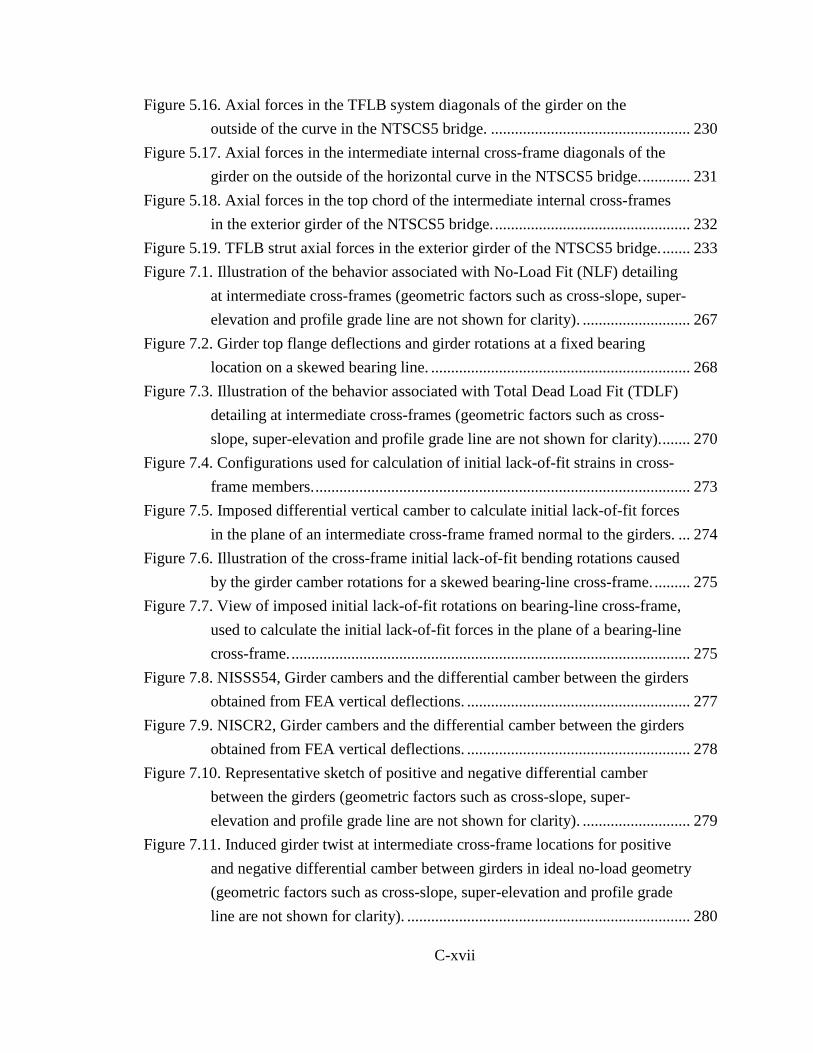
Figure 5.16. Axial forces in the TFLB system diagonals of the girder on the outside of the curve in the NTSCS5 bridge. .................................................. 230

Figure 5.17. Axial forces in the intermediate internal cross-frame diagonals of the girder on the outside of the horizontal curve in the NTSCS5 bridge. ............ 231

Figure 5.18. Axial forces in the top chord of the intermediate internal cross-frames in the exterior girder of the NTSCS5 bridge. ................................................. 232

Figure 5.19. TFLB strut axial forces in the exterior girder of the NTSCS5 bridge. ....... 233

Figure 7.1. Illustration of the behavior associated with No-Load Fit (NLF) detailing at intermediate cross-frames (geometric factors such as cross-slope, super-elevation and profile grade line are not shown for clarity). ........................... 267

Figure 7.2. Girder top flange deflections and girder rotations at a fixed bearing location on a skewed bearing line. ................................................................. 268

Figure 7.3. Illustration of the behavior associated with Total Dead Load Fit (TDLF) detailing at intermediate cross-frames (geometric factors such as cross-slope, super-elevation and profile grade line are not shown for clarity). ....... 270

Figure 7.4. Configurations used for calculation of initial lack-of-fit strains in cross-frame members. .............................................................................................. 273

Figure 7.5. Imposed differential vertical camber to calculate initial lack-of-fit forces in the plane of an intermediate cross-frame framed normal to the girders. ... 274

Figure 7.6. Illustration of the cross-frame initial lack-of-fit bending rotations caused by the girder camber rotations for a skewed bearing-line cross-frame. ......... 275

Figure 7.7. View of imposed initial lack-of-fit rotations on bearing-line cross-frame, used to calculate the initial lack-of-fit forces in the plane of a bearing-line cross-frame. .................................................................................................... 275

Figure 7.8. NISSS54, Girder cambers and the differential camber between the girders obtained from FEA vertical deflections. ........................................................ 277

Figure 7.9. NISCR2, Girder cambers and the differential camber between the girders obtained from FEA vertical deflections. ........................................................ 278

Figure 7.10. Representative sketch of positive and negative differential camber between the girders (geometric factors such as cross-slope, super- elevation and profile grade line are not shown for clarity). ........................... 279

Figure 7.11. Induced girder twist at intermediate cross-frame locations for positive and negative differential camber between girders in ideal no-load geometry (geometric factors such as cross-slope, super-elevation and profile grade line are not shown for clarity). ....................................................................... 280

C-xviii

Figure 7.12. NISSS54, Deflected shape under steel dead load for different types of detailing methods (magnified by 10x). .......................................................... 282

Figure 7.13. NISSS54, Deflected shape under total dead load for different types of detailing methods (magnified by 10x). .......................................................... 283

Figure 7.14. NISSS54, steel dead load girder layovers associated with different types of detailing methods. ...................................................................................... 284

Figure 7.15. NISSS54, total dead load girder layovers associated with different types of detailing methods. ...................................................................................... 285

Figure 7.16. NISSS54, Normalized maximum amplitude of the component axial forces in each of the cross-frames under total dead load (NLF detailing). .... 288

Figure 7.17. NISSS54, maximum amplitude of the component axial forces in each of the cross-frames under total dead load (NLF detailing). ........................... 289

Figure 7.18. NISSS54, maximum amplitude of the component axial forces in each of the cross-frames under total dead load plus the TDLF detailing effects. .. 290

Figure 7.19. NISCR2, maximum amplitude of the component axial forces in each of the cross-frames under total dead load (NLF detailing). ........................... 291

Figure 7.20. NISCR2, maximum amplitude of the component axial forces in each of the cross-frames under total dead load plus the TDLF detailing effects. .. 291

Figure 7.21. NISSS54, Vertical deflections under total dead load associated with different detailing methods. ........................................................................... 293

Figure 7.22. NISCR5, Vertical deflections under total dead load associated with different detailing methods. ........................................................................... 294

Figure 7.23. Illustrative curved girder deformations under dead loads. ......................... 295

Figure 7.24. NISSS54, top flange stresses under total dead load for different detailing methods. .......................................................................................... 298

Figure 7.25. NISCR2, Top flange stresses under total dead load for different detailing methods. .......................................................................................... 300

Figure 7.26. NISCR2, vertical displacements at the mid-span of Girder G1 versus the fraction of the total dead load for different detailing methods. ................ 302

Figure 7.27. NISCR5, vertical displacements at the mid-span of Girder G1 versus the fraction of the total dead load for different detailing methods. ................ 302

Figure 7.28. NISSS54, Girder camber profiles, obtained from different analysis solutions. ........................................................................................................ 304

C-xix

Figure 7.29. NISSS54, total dead load vertical deflections and top flange stresses associated with NLF and TDLF detailing where the cambers are set based on line girder analysis results. .............................................................. 306

Figure 7.30. NISCR2, Total dead load cambers obtained from line girder and finite element analysis solutions. ............................................................................. 309

Figure 7.31. NISSS54, total dead load vertical deflections and top flange stresses associated with NLF and TDLF detailing where the cambers are set based on line girder analysis results. .............................................................. 311

Figure 9.1. EISCS3 bridge layout. .................................................................................. 330

Figure 9.2. Intermediate cross-frame configurations implemented in the analyses. ...... 331

Figure 9.3. Comparison of stresses and relative lateral displacements for EISCS3 with and without a top chord in the cross-frames (Analysis 1 does not have a top chord whereas Analysis 2 has a top chord). ................................. 332

Figure 9.4. Typical connection details used for skewed cross-frames. .......................... 333

Figure 9.5. Improved connection details used for skewed cross-frames. ....................... 334

Figure 9.6. NISCR11, undeflected and deflected geometry under total dead load (Magnified by 20x). ....................................................................................... 336

Figure 9.7. NISCR11, total dead load vertical displacements from first- and second-order analyses. ................................................................................................ 336

Figure 9.8. NISCR11, Total dead load layovers in Girder G1 from first- and second-order analyses. ................................................................................................ 337

Figure 9.9. NISCR11, Girder G1 total dead load radial displacements from first- and second-order analyses.............................................................................. 337

Figure 9.10. NISCR11, Girder G9 total dead load radial displacements from first- and second-order analyses.............................................................................. 338

Figure 9.11. NISCR11, Girder G1 top flange stresses under total dead load. ................ 338

Figure 9.12. Detail of non-collinear and collinear external diaphragms in tub-girder bridges. ........................................................................................................... 340

C-xxi

List of Tables

Table 2.1. Values of the C coefficient. ............................................................................. 14

Table 2.2. AASHTO constructability checks using simplified line-girder (V-load) analysis with global amplification factor and refined 3D FE analysis results. .............................................................................................................. 75

Table 4.1. Primary factor ranges and levels for the NCHRP 12-79 main analytical study. .............................................................................................................. 138

Table 4.2. Overall summary of New, Existing and eXample I-girder bridges. .............. 177

Table 4.3. Overall summary of New, Existing and eXample tub-girder bridges. .......... 178

Table 5.1. I-girder bridge percent normalized mean errors compared to 3D second-order elastic FEA for major-axis bending stresses (fb) and vertical displacements (∆z). ......................................................................................... 183

Table 5.2. Number of I-girder bridges within specified error ranges for major-axis bending stress and vertical displacement for each of the types of bridges considered. ..................................................................................................... 196

Table 5.3. Worst-case I-girder bridge scores for major-axis bending stress and vertical displacement. ..................................................................................... 197

Table 5.4. Mode of I-girder bridge scores for major-axis bending stress and vertical displacement. .................................................................................................. 198

Table 5.5. Generalized I-girder bridge scores. ................................................................ 200

Table 5.6. Cross-frame forces predicted with the 2D-grid and the 3D FEA .................. 206

Table 5.7. Tub-girder bridge percent normalized mean errors compared to geometric nonlinear elastic 3D FEA for major-axis bending stresses (fb), vertical displacements (∆z) and torsional moment (T). .................................. 212

Table 5.8. Tub-girder bridge percent errors for maximum values of responses compared to geometric nonlinear elastic 3D FEA for the bracing system forces. ............................................................................................................. 213

Table 5.9. Number of tub-girder bridges within specified error ranges for major-axis bending stress and vertical displacement for each of the types of bridges considered. ..................................................................................................... 220

Table 5.10. Tub-girder bridge worst-case scores for major-axis bending stress, vertical displacements, and torques................................................................ 220

Table 5.11. Mode of tub-girder bridge scores for major-axis bending stress, vertical displacements, and torques............................................................................. 221

C-xxii

Table 5.12. Number of tub-girder bridges within specified error ranges for the maximum values of the bracing system forces for each of the types of bridges considered. ......................................................................................... 222

C-1

Executive Summary

In current practice (2012), the construction of curved and/or skewed steel girder

bridges is sometimes hampered by misconceptions regarding the three-dimensional

behavior of these structures. The deflections of curved and skewed girder bridges

intrinsically involve torsion of the bridge cross-section and of the individual girders. The

resulting 3D movements can affect the fit-up of cross-frames or diaphragms during the

steel erection. Furthermore, they can influence the control of the deck thickness, the final

deck slopes and superelevations, the dead load rotations at bearings, the alignment of

units at deck joints, and the matching of stages in phased construction projects.

Depending on the severity of the bridge geometric conditions and the specific needs

regarding the geometry control, a simple analysis solution may be sufficient to assess

these considerations or a more refined analysis may be necessary.

This document provides guidelines for the selection of analytical methods for the

design of skewed and/or horizontally curved steel girder bridges for construction. Both

steel I- and tub-girder bridges are addressed. Emphasis is placed on the assessment of

when simplified 1D or 2D analysis methods are sufficient, and when 3D methods may be

more appropriate for assessment of constructability demands and prediction of the

constructed geometry of curved and/or skewed structures.

The report first scrutinizes a number of commonly used 1D, 2D and 3D analysis

idealizations to provide a detailed understanding of the underlying assumptions and basic

limits of applicability of the methods. A number of established extensions of typical 1D

and 2D analyses are discussed that allow the engineer to obtain the broadest potential

range of information with these methods when they are applicable. Secondly, several key

geometry related bridge indices are identified that can be utilized as aids to identify when

different simplified approximations may be suspect. These indices are then used as a part

of guidelines for the selection of analytical methods.

Interestingly, although vertical deflections and girder major-axis bending stresses

may be estimated with reasonable accuracy in a large number of situations, the cross-

C-2

frame forces and girder flange lateral bending stresses in skewed I-girder bridges are

essentially impossible to determine with any confidence using 1D line-girder and

conventional 2D-grid analysis methods. The problems lie in general with the lack of any

ability to capture transverse load paths using the 1D methods, and the gross errors

associated with neglecting the true girder warping torsion stiffness and the cross-frame

stiffness characteristics in conventional 2D-grid methods. Modifications to conventional

2D-grid analysis methods are provided, however, which result in reliable predictions over

a wide range of I-girder bridges.

This study also addresses the difficult questions of what types of cross-frame

detailing are most effective for different bridge geometries, and when should locked-in

force effects due to the detailing of cross-frames be considered in the calculation of I-

girder bridge responses. Recommended procedures are provided for determining locked-

in force effects for cases in which these effects need to be included. In addition,

guidelines are provided for the selection of cross-frame detailing methods as a function of

the bridge geometry.

Lastly, the report discusses a number of design and construction considerations

that can be implemented to alleviate the demands on the methods of structural analysis by

improving the bridge behavior, various problematic physical characteristics, details and

practices are outlined, and important potential pitfalls associated with 1D, 2D and 3D

analysis techniques are highlighted.

C-3

1. Introduction

1.1 Problem Statement

Curved and/or skewed steel I- and tub-girder bridges can experience significant

3D deflections and rotations. In general, 3D deflections and rotations must be considered

in the design, detailing and construction engineering of these bridge types. The 3D

movements can affect the fit up of cross-frames or diaphragms during the steel erection.

Furthermore, they can influence the control of the bridge geometry, including the deck

thickness, the final deck slopes and superelevations, the dead load rotations at the

bearings, the alignment of units at deck joints, and the matching of stages in phased

construction projects. Depending on the severity of the bridge geometric conditions and

the specific needs regarding the geometry control, a simple analysis solution may be

sufficient or a more refined analysis may be necessary.

Longer span bridges tend to be affected more substantially by dead load effects,

potentially resulting in more significant stability considerations during construction. In

curved and/or skewed structures, these effects are manifested predominantly in the

second-order amplification of the deflections and internal stresses. During intermediate

erection stages, it is important that the physical component stresses are limited, including

any significant second-order effects, such that there is no significant onset of inelastic

deformations and no component strength limits are exceeded. Conversely, shorter span

bridges tend to be dominated more by live load effects; thus, these bridges tend to be less

affected by construction loading conditions.

Longer span bridges generally exhibit larger deflections; hence, the accuracy of

the deflection predictions can be more critical. Shorter span bridges have smaller

deflections and are thus less apt to experience problems due to the movements of the

structure during construction. One of the key instances where the deflections during

construction can be a factor is during the placement of the deck. Inaccurate prediction of

the system deflections can result in over-run or under-run of the deck thickness,

deviations from intended deck slopes and superelevations, local dips in deck elevation

that are susceptible to ponding, unintended bearing rotations, misalignment of units at

C-4

deck joints, and/or mismatched stages in phased construction projects. Since the overall

deflections are larger in longer span bridges, the relative deflections that drive the above

concerns are also larger. Control of the geometry during the placement of the deck is an

essential consideration in the construction of curved and skewed girder bridges,

particularly for bridges with longer spans.

Structural engineers currently have a wide array of approximate and refined

analysis and design tools at their disposal. It is important that the right tool is selected for

a given bridge. In addition, there are a number of specific cross-frame detailing practices

typically used to economically control, i.e., to compensate for, the 3D deflections and

rotations in curved and skewed I-girder bridges. The application of and the implications

of these practices need to be better understood so that they can be applied in the most

effective ways.

Bridges with significant span lengths, curvature and skew generally require

careful planning of the erection procedures and sequences such that lifting and fit-up of

their spatially deformed components and subassemblies is achievable. Longer and/or

wider bridges also may require placement of the deck in multiple stages. Setup of the

concrete from prior stages, and in some cases during the current stage, can have a

significant influence on the final geometry and on the ultimate performance of the deck.

Some wide bridges may require construction in multiple longitudinal phases, with the

corresponding problems of connecting new steel to a completed structure, and the

matching of deck elevations between adjacent phases. On the other hand, shorter bridges

with minor curvature and skew often can be built with less attention to the construction

engineering. With respect to all the above considerations, it is important that the

appropriate level of effort is applied for the task at hand.

1.2 Objectives

This document outlines the key characteristics of various simplified 1D and 2D

analysis methods. It provides guidelines for when these methods are sufficient as well as

recommendations for when more sophisticated 3D analysis capabilities may be warranted

for assessment of the constructability and prediction of the final constructed geometry of

C-5

curved and/or skewed steel girder bridges. Both I-girder and tub-girder bridges are

addressed. These guidelines are based on extensive information collected from prior and

current research, input from bridge owner and consultant policies and practices, and

fundamental studies of the accuracy of the simplified methods of analysis conducted by

NCHRP Project 12-79, “Guidelines for Analytical Methods and Erection Engineering of

Curved and Skewed Steel Deck-Girder Bridges.” This report focuses on the accuracy of

analysis methods commonly used to determine the strength, stability, and constructability

of curved and/or skewed steel girder bridges under the action of their self-weight and

various loads imposed during construction operations. In addition, a number of

improvements are recommended to conventional analysis techniques that are necessary to

eliminate several critical flaws identified by the NCHRP Project 12-79 research.

1.3 Organization

This report is subdivided into eleven main chapters. Chapter 2 aims to establish

the framework for the discussions in the other chapters by providing an overview of the

common structural analysis tools available in current (2012) practice for analysis of

curved and/or skewed steel girder bridges. Namely, these are:

1) Line-girder (1D) methods,

2) 2D-grid methods,

3) 2D-frame methods,

4) Plate and eccentric beam methods,

5) Conventional 3D-frame methods,

6) Thin-walled open-section (TWOS) 3D-frame methods, and

7) 3D Finite Element Analysis (FEA) methods.

The essential idealizations and approximations are summarized for each of these

methods. In addition, Chapter 2 discusses specific hand calculation equations commonly

used with the 1D and 2D methods, second-order amplification estimates for displace-

ments and stresses in cases where stability effects may be important, and analysis of

composite action between the bridge deck and the steel structure, including staged deck

placement and consideration of early stiffness and strength gains of the concrete. Chapter

C-6

2 closes with a discussion of response attributes that generally cannot be captured by 1D

and 2D methods. Of course, in cases where these attributes are not an important factor in

the response of the structure, these limitations do not significantly impact the accuracy of

the analysis. However, clearly if any of these attributes is expected to be an important

contributor to particular structural actions, the engineer must utilize an analysis method

capable of capturing the contribution when evaluating these actions.

Chapter 3 defines several key indices identified by NCHRP 12-79 as the most

useful for characterizing the importance of curvature and skew on the accuracy of

analysis methods for steel girder bridges. Subsequently, these indices are employed as

aids to identify when simpler methods of analysis are sufficient as well as when more

sophisticated methods should be applied. In addition, this chapter comments on the broad

range of factors that generally can influence the detailed behavior of these types of

structures.

Chapter 4 provides an overview of the NCHRP 12-79 studies leading to the

recommendations of this report. The emphasis of this chapter is on the design and

development of a large parametric study of curved and skewed I- and tub-girder bridge

systems conducted in the NCHRP research.

Chapter 5 summarizes the core results of the parametric studies conducted by

NCHRP 12-79. A scoring method is introduced and utilized to quantify the ability of the

different methods of analysis for predicting essential responses. Unfortunately, for a

number of responses pertaining to I-girder bridges, the accuracy of commonly used

(conventional) simplified methods is essentially binary. That is, either a given method

works well or its usage is very suspect. The reasons for this behavior are explained in

Chapter 6. Chapter 6 also recommends specific improvements to conventional 2D-grid

methods for the analysis of I-girder bridges developed in the NCHRP 12-79 research.

Chapter 7 addresses the consideration of locked-in force effects associated with

cross-frame detailing methods commonly used to achieve approximately plumb girder

webs at targeted stages of I-girder bridge construction. The highly complex bridge

behavior associated with these relatively simple cross-frame detailing practices is

C-7

explained through a series of examples. Specific conditions are shown where the locked-

in forces from cross-frame detailing should be considered in the design. In addition,

specific analysis procedures for determining the locked-in force effects are presented. It

is emphasized that these locked-in forces are beneficial in that they provide a simple and

cost-effective means of achieving plumb webs under a given dead load condition.

However, in certain cases, these effects need to be considered in determining vertical

deflections and setting cambers, and in evaluating the structural resistances. Lastly,

Chapter 7 discusses several special cases where a 1D (line-girder) analysis (with proper

extensions where needed) tends to produce sufficiently accurate results for all the

essential response quantities (including locked-in forces), as well as when an accurate

structural analysis without including the locked-in forces potentially can be used to

estimate the maximum cross-frame forces and girder flange lateral bending stresses in I-

girder bridges.

In many situations, the need for a more sophisticated type of analysis can be

reduced or eliminated by intelligent and prudent decisions made during the design and

construction engineering. Chapter 8 discusses a number of considerations that can ease

the demands on the structural analysis via improved structural behavior.

Chapter 9 discusses specific characteristics, practices and details that can lead to

major difficulties in the ability to predict the response of the structure during construc-

tion, and therefore should be used very carefully or sparingly if they are used at all.

Lastly, Chapter 10 summarizes key pitfalls in 1D, 2D and 3D methods of analysis for

construction engineering of curved and/or skewed girder bridges. Chapter 11 summarizes

the recommendations of this report in a concise form.

C-8

1.4 Scope and Intended Audience of this Report

This report presents the results of the NCHRP 12-79 research on methods of

analysis in a summary form for engineers interested in accessing the details of the

research behind the subject recommendations. Readers interested in a concise implemen-

tation of the NCHRP 12-79 recommendations in a code-type format oriented toward

current practice should first view the companion Task 9 report “Recommendations for

Construction Plan Details and Level of Construction Analysis.” Readers interested in a

concise summary of the improvements to simplified methods of analysis and their

application, should first consult the NCHRP 12-79 Final Report.

C-9

2. Overview of Methods (Types) of Analysis

2.1 Line-Girder (1D) Analysis

Line-girder analysis is the most basic method used in the engineering of girder

bridges. In this method, the bridge girders are analyzed individually, and their interaction

with the bracing system is ignored or accounted for only in a coarse fashion. The loads

during steel erection are commonly taken as those acting directly on each girder, but

various approaches are used for distributing the subsequent dead loads. NHI (2007)

suggests that when the width of the deck is constant, the girders are parallel and have

approximately the same stiffness, and the number of girders is not less than four, the

permanent load of the wet concrete deck may be distributed equally to each of the girders

in the cross-section. Article 4.6.2.2.4 of (AASHTO, 2010) indicates that wearing surface

and other distributed loads may be assumed uniformly distributed to each girder in the

cross-section of curved steel bridges. However, (NHI, 2011) emphasizes that heavier DC2

line loads such as parapets, barriers, sidewalks or sound walls should not be distributed

equally to all the girders. If the overhang widths and/or the concrete barrier loads are

large, engineers commonly use the lever rule (AASHTO, 2010) to distribute the overhang

and barrier loads to the girders. Alternatively, some state DOTs assign 60 % of the barrier

weight to the exterior girders and 40 % to the adjacent interior girders (NHI, 2007). If the

lever rule is used, the portion of the dead load assigned to the fascia girders is increased,

while the loads on the interior girders are reduced. NHI (2010) points out that estimating

the distribution of DC2 line loads to the individual girders for line girder analysis is

particularly difficult in skewed bridges since the loads may only be on one side of the

bridge over significant portions of the span. In addition, NHI (2007) indicates equal

distribution of distributed loads can be suspect for skews larger than 10 degrees.

Considering all these factors, the distributed dead loads were assigned to the girders

based on tributary area in the 1D analyses conducted by the NCHRP 12-79 project team.

Parapet loads were considered in the design of parametric study bridges in the NCHRP

12-79 research, but these bridge designs were conducted using 2D-grid and Plate-

eccentric beam analysis procedures discussed subsequently.

C-10

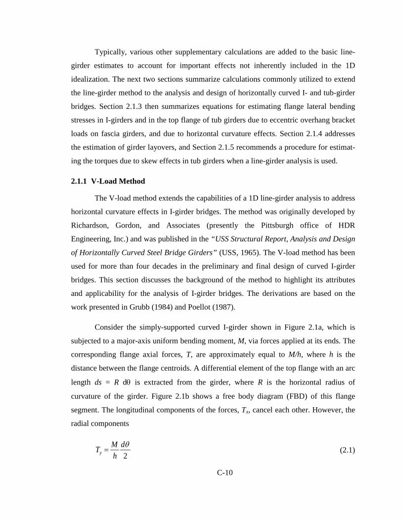
Typically, various other supplementary calculations are added to the basic line-

girder estimates to account for important effects not inherently included in the 1D

idealization. The next two sections summarize calculations commonly utilized to extend

the line-girder method to the analysis and design of horizontally curved I- and tub-girder

bridges. Section 2.1.3 then summarizes equations for estimating flange lateral bending

stresses in I-girders and in the top flange of tub girders due to eccentric overhang bracket

loads on fascia girders, and due to horizontal curvature effects. Section 2.1.4 addresses

the estimation of girder layovers, and Section 2.1.5 recommends a procedure for estimat-

ing the torques due to skew effects in tub girders when a line-girder analysis is used.

2.1.1 V-Load Method

The V-load method extends the capabilities of a 1D line-girder analysis to address

horizontal curvature effects in I-girder bridges. The method was originally developed by

Richardson, Gordon, and Associates (presently the Pittsburgh office of HDR

Engineering, Inc.) and was published in the “USS Structural Report, Analysis and Design

of Horizontally Curved Steel Bridge Girders” (USS, 1965). The V-load method has been

used for more than four decades in the preliminary and final design of curved I-girder

bridges. This section discusses the background of the method to highlight its attributes

and applicability for the analysis of I-girder bridges. The derivations are based on the

work presented in Grubb (1984) and Poellot (1987).

Consider the simply-supported curved I-girder shown in Figure 2.1a, which is

subjected to a major-axis uniform bending moment, M, via forces applied at its ends. The

corresponding flange axial forces, T, are approximately equal to M/h, where h is the

distance between the flange centroids. A differential element of the top flange with an arc

length ds = R dθ is extracted from the girder, where R is the horizontal radius of

curvature of the girder. Figure 2.1b shows a free body diagram (FBD) of this flange

segment. The longitudinal components of the forces, Tx, cancel each other. However, the

radial components

2θd

hMTy = (2.1)

C-11

are additive. Therefore, a uniformly distributed internal force

RhM

dsT

q y ==2

(2.2)

transferred via the web, is necessary to balance these components. Upon multiplying both

sides of this equation by the radius R, one can observe that the flange axial force, T, is

equal to qR.

(a) Axial forces in the top flange due to uniform moment

(b) Free body diagram of the flange segment

Figure 2.1. Curved girder subjected to a uniform major-axis bending moment.

The above uniformly distributed force, q, subjects the flanges to lateral bending.

Hence, in a two-girder system such as the one depicted in Figure 2.2a, the flanges behave

like continuous-span beams in the lateral direction, while the cross-frames act like the

continuous-span beam supports. The girders G1 and G2 in this figure are subjected to

major-axis bending moments M1(x) and M2(x), respectively, where x is the coordinate

measured along the arc length of the girders. For equilibrium of the exterior girder at the

first intermediate cross-frame in Figure 2.2b the reaction at the level of the cross-frame

chords, H1, must be approximately equal to q1Lb1h/hCF, where hCF is the depth between

C-12

the centerline of the cross-frame chords and Lb1 is the distance between cross-frames

measured along the centerline of G1 (assumed constant). By substituting q1 = M1/R1h,

one obtains

CF

b

hRLMH

1

111 = (2.3)

where R1 is taken as the radius of curvature of the girder at location 1. The moment in

this equation, M1, is taken as the value at the cross-frame position, i.e., M1 = M1(Lb1).

(a) Plan view of the two-girder system

(b) Free body diagram of the first intermediate cross-frame

Figure 2.2. Interaction of forces in a curved girder system.

The reaction at the bottom chord level is the same as H1, but is in the opposite

direction, since the moment causes compression in the top flange and is assumed to cause

an equal tension in the bottom flange. Similarly, for the interior girder, G2, the reaction,

H2, may be written as

C-13

CF

bb hR

LMLqH2

22222 == (2.4)

where M2 = M2(Lb2). Note that Lb1/R1 = Lb2/R2 may be written as a common value Lb/R,

such that H1 = M1 Lb/RhCF and H2 = M2 Lb /RhCF.

In the cross-frame shown in Figure 2.2b, moment equilibrium requires that

b

CFCF LRS

MMS

hHHV 2121

1+

=+

=)(

(2.5)

These vertical forces are a direct effect of the horizontal curvature, and are known as the

V-loads. In Eq. 2.5, the subscript CF1 is used to emphasize that this is a load at the first

intermediate cross-frame position. Similarly, the loads at the other cross-frame positions

can be found by substituting the corresponding moments M1 and M2, accordingly. In the

exterior girder, G1, the additional moments caused by the downward action of the V-

loads, M1s, add to the moments produced directly by the gravity loads, M1p. In the interior

girder, G2, these loads are in opposite directions, so the resulting moments are subtracted

from the gravity load moments. Therefore, the total moment in a particular cross-section

of girder G1, M1, is equal to M1p + M1s. Likewise, for the interior girder, M2 = M2p + M2s.

Moreover, at any cross-frame position, M1s ≅ −M2s (L1/L2), where L1 and L2 are the arc-

span lengths of G1 and G2, respectively. For practical cases, the term (L1/L2) is close to

one, so M1s ≈ −M2s. Given this approximation, the sum of the total moments in G1 and

G2, M1 + M2, may be taken as M1p + M2p. Substituting this result into Eq. 2.5, one has

1 21

+= p p

CFb

M MV

RS L (2.6)

Given the above approximations, the girders can be analyzed independently using

a line-girder analysis. The curved girders are represented with equivalent straight girders

of length L1 and L2, and they are subjected to the gravity loads plus the V-loads.

The above development can be extended to consider cases with more than two

girders. As explained by Poellot (1987), the V-loads in a multi-girder system are the total

C-14

vertical loads delivered to the girders from the cross-frames (equal to the difference in the

cross-frame shear forces on the interior girders). The V-load delivered to the girder

farthest from the bridge centerline is calculated as

b

p

LCRSM

V ∑= (2.7)

The V-loads delivered to the other girders are assumed to vary linearly between a value

of zero for any girder at the bridge centerline to the maximum value predicted by Eq. 2.7

for the girder(s) farthest from the centerline. The constant C in this equation depends on

the number of girders in the structure. Table 2.1 shows the values of C for systems with

up to ten girders. These constants are derived based on the above assumption.

Table 2.1. Values of the C coefficient.

Girders Coefficient 2 1 3 1 4 10/9 5 5/4 6 7/5 7 14/9 8 12/7 9 15/8 10 165/81

The V-load idealization basically assumes: (1) approximately equal vertical

stiffness of all the girders (defined by a unit load applied at a given cross-frame location,

divided by the vertical deflection at that location due to the unit load), and (2) a linear

variation in vertical displacements across the bridge cross-section due to overall torsion.

In general, the V-load method is reasonably accurate for cases that closely satisfy the

above assumptions used in its derivation. However, for bridges with skewed supports,

staggered cross-frame patterns, etc., a line-girder analysis based on the V-load method

may not be sufficient. For those cases, a 3D FEA model, or 2D-grid model with the

recommended improvements discussed in Chapter 6 (which captures the interaction

C-15

between the structural components more accurately than conventional 2D-grid methods),

may be required. These aspects are discussed in the subsequent sections of this report.

2.1.2 M/R Method

The M/R method is a simplified tool for estimating the torsional effects due to

curvature in general box girders. This method, which was first introduced by Tung and

Fountain (1970), applies an equivalent distributed torsional moment M /R to an individual

girder, where M is the major-axis bending moment and R is the radius of curvature. This

method assumes that each of the box-girders in the bridge cross-section deforms

independently from the other girders for a given span. That is, any interaction between

the girders due to their interconnection via the bridge deck and/or intermediate external

diaphragms is neglected. The assumptions behind the method are explained by Figure

2.3, which shows a free-body diagram for a box girder differential segment ds. The

equivalent force at the flange levels, M/h, is the same as the force T in Figure 2.1.

ds

h

dθ

R

M M

Mh

Plan view

Elevation view

Figure 2.3. Force equilibrium in a segment of a box girder.

C-16

As in the V-load method developments explained in Section 2.1.1, the unbalanced

flange-level lateral force due to the curvature at the given segment ds = R dθ is obtained

as

Rds

hMd

hMTy =

=

2θ2 (2.8)

By dividing both sides of this equation by ds, one obtains the equivalent distributed

lateral loads at the top and bottom of the section

RhM

dsRds

hM

dsHq ===

1 (2.9)

These loads produce an equivalent distributed torsional moment M/R shown in Figure

2.4, which is identical to the effect of the flange-level distributed lateral load shown in

the previous section.

MRh

MRh

hMR

Figure 2.4. M/R torsional moment.

Next, given the specific M/R method assumption of no interactions between the girders

along the span length, the internal torsional moment at a given position s can be found,

considering a free body diagram of the girder segment from zero to s, and assuming

cos(L/R) = 1.0 (i.e., assuming a small subtended angle over the length s), as

( ) ( )∫−=

sds

RsMTsT

0support (2.10)

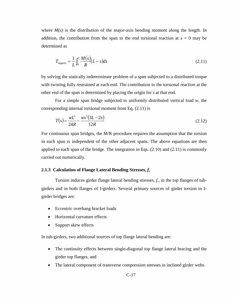
C-17

where M(s) is the distribution of the major-axis bending moment along the length. In

addition, the contribution from the span to the end torsional reaction at s = 0 may be

determined as

( )( )dssLR

sML

TL

−= ∫0support1

(2.11)

by solving the statically indeterminate problem of a span subjected to a distributed torque

with twisting fully restrained at each end. The contribution to the torsional reaction at the

other end of the span is determined by placing the origin for s at that end.

For a simple span bridge subjected to uniformly distributed vertical load w, the

corresponding internal torsional moment from Eq. (2.11) is

( ) ( )R

sLwsR

wLsT12

2324

23 −−= (2.12)

For continuous span bridges, the M/R procedure requires the assumption that the torsion

in each span is independent of the other adjacent spans. The above equations are then

applied to each span of the bridge. The integration in Eqs. (2.10) and (2.11) is commonly

carried out numerically.

2.1.3 Calculation of Flange Lateral Bending Stresses, f

Torsion induces girder flange lateral bending stresses, f, in the top flanges of tub-

girders and in both flanges of I-girders. Several primary sources of girder torsion in I-

girder bridges are:

• Eccentric overhang bracket loads

• Horizontal curvature effects

• Support skew effects

In tub-girders, two additional sources of top flange lateral bending are:

• The continuity effects between single-diagonal top flange lateral bracing and the

girder top flanges, and

• The lateral component of transverse compression stresses in inclined girder webs.

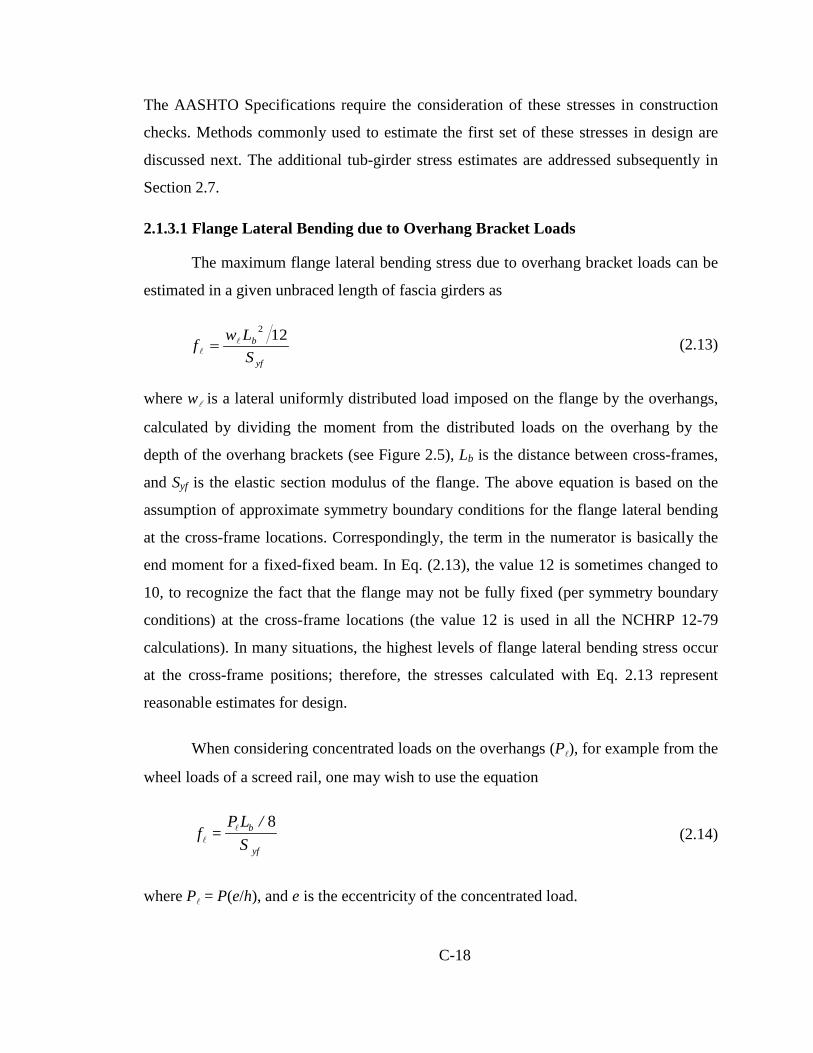
C-18

The AASHTO Specifications require the consideration of these stresses in construction

checks. Methods commonly used to estimate the first set of these stresses in design are

discussed next. The additional tub-girder stress estimates are addressed subsequently in

Section 2.7.

2.1.3.1 Flange Lateral Bending due to Overhang Bracket Loads

The maximum flange lateral bending stress due to overhang bracket loads can be

estimated in a given unbraced length of fascia girders as

yf

b

SLw

f122

= (2.13)

where w is a lateral uniformly distributed load imposed on the flange by the overhangs,

calculated by dividing the moment from the distributed loads on the overhang by the

depth of the overhang brackets (see Figure 2.5), Lb is the distance between cross-frames,

and Syf is the elastic section modulus of the flange. The above equation is based on the

assumption of approximate symmetry boundary conditions for the flange lateral bending

at the cross-frame locations. Correspondingly, the term in the numerator is basically the

end moment for a fixed-fixed beam. In Eq. (2.13), the value 12 is sometimes changed to

10, to recognize the fact that the flange may not be fully fixed (per symmetry boundary

conditions) at the cross-frame locations (the value 12 is used in all the NCHRP 12-79

calculations). In many situations, the highest levels of flange lateral bending stress occur

at the cross-frame positions; therefore, the stresses calculated with Eq. 2.13 represent

reasonable estimates for design.

When considering concentrated loads on the overhangs (P), for example from the

wheel loads of a screed rail, one may wish to use the equation

8= b

yf

P L /f

S

(2.14)

where P = P(e/h), and e is the eccentricity of the concentrated load.

C-19

Figure 2.5. Determination of the uniformly distributed load w.

It is important generally to ensure that the bracket loads applied to the I-girder

web are sufficiently close to the bottom flange such that there is negligible distortion of

the web from the reaction at the bottom of the overhang bracket (Ohio DOT, 2008;

Roddis et al., 2005). Note that if the bracket cannot be located close to the bottom flange

(approximately 6 inches), then it may be necessary to verify that the bracket load will not

distort the web, or some type of additional bracing support may be required.

2.1.3.2 Flange Lateral Bending due to Horizontal Curvature

The flange lateral bending stresses due to horizontal curvature can be estimated at

the cross-frame locations using the formula

yf

b

SRhMLf 122

= (2.15)

This equation is essentially the same form as Eq. 2.13, but with an assumed uniformly

distributed lateral load, q = M/Rh, derived from the V-load method, and substituted for w

(see Section 2.1.1). In Eq. 2.15, the moment M typically is taken as the total major-axis

bending moment at a particular cross-frame location resulting from the action of the

gravity loads and the V-loads, i.e., M = Mp + Ms. In the fascia girder on the outside of the

curve, the combined effects of the horizontal curvature and the overhang bracket loads

are considered simultaneously by adding the results of Eqs. (2.13) and (2.15). Similar to

the application of Eq. (2.13), engineers sometimes use a coefficient of 10 rather than 12

C-20

in Eq. (2.15), as an attempt to ensure a conservative estimate of the flange lateral bending

stress. The coefficient 12 is used in all the NCHRP 12-79 studies,

In Eq. 2.15, the elastic section modulus for a typical rectangular flange, Syf, is

equal to (tf bf3/12)/(bf /2), where bf and tf are the flange width and thickness, respectively.

Since the flange area, Af , is equal to bf tf , the section modulus can be expressed as Sy =

Af·bf/6. In addition, the moment, M, is equal to fb Sx, where fb is the major-axis bending

stress and Sx is the strong-axis elastic section modulus to the flange under consideration.

Substituting these parameters into Eq. 2.15, the flange lateral bending stress can be

expressed as

=2b x b b

f o f

f S L Lf

A h R b (2.16)

This form of the equation for f highlights the fundamental factors influencing the flange

lateral bending stresses induced by the horizontal curvature (in the context of the above

idealizations). Note that if the girder is doubly-symmetric and the contribution of the web

to the girder moment of inertia is relatively small, Sx/(Af ho) ≈ 1. In this case, the f stress

is simply equal to one-half of the product of the major-axis bending stress fb, the sub-

tended angle between the cross-frames Lb/R, and the flange length-to-width ratio Lb/bf.

2.1.3.3 Flange Lateral Bending due to Skew Effects

There is limited guidance in current practice on how to calculate the f stresses

resulting from skew effects when an I-girder bridge is evaluated using a line-girder or a

conventional 2D-grid analysis. In lieu of providing a predictor method, AASHTO LRFD

Article C6.10.1 states:

“In the absence of calculated values of f from a refined analysis, a suggested estimate for

the total f in a flange at a cross-frame or diaphragm due to the use of discontinuous

cross-frame or diaphragm lines is 10.0 ksi for interior girders and 7.5 ksi for exterior

girders. These estimates are based on a limited examination of refined analysis results for

bridges with skews approaching 60 degrees from normal and an average D/bf ratio of

approximately 4.0. In regions of the girders with contiguous cross-frames or diaphragms,

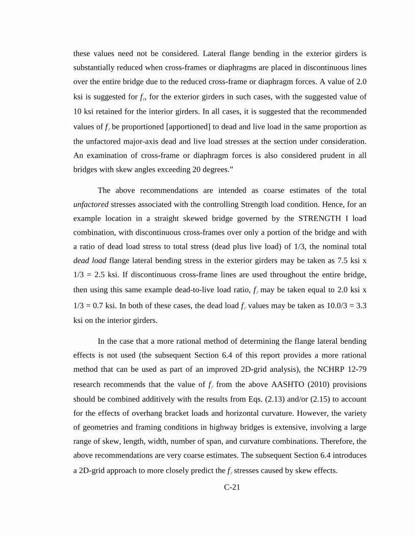
C-21

these values need not be considered. Lateral flange bending in the exterior girders is

substantially reduced when cross-frames or diaphragms are placed in discontinuous lines

over the entire bridge due to the reduced cross-frame or diaphragm forces. A value of 2.0

ksi is suggested for f, for the exterior girders in such cases, with the suggested value of

10 ksi retained for the interior girders. In all cases, it is suggested that the recommended

values of f be proportioned [apportioned] to dead and live load in the same proportion as

the unfactored major-axis dead and live load stresses at the section under consideration.

An examination of cross-frame or diaphragm forces is also considered prudent in all

bridges with skew angles exceeding 20 degrees.”

The above recommendations are intended as coarse estimates of the total

unfactored stresses associated with the controlling Strength load condition. Hence, for an

example location in a straight skewed bridge governed by the STRENGTH I load

combination, with discontinuous cross-frames over only a portion of the bridge and with

a ratio of dead load stress to total stress (dead plus live load) of 1/3, the nominal total

dead load flange lateral bending stress in the exterior girders may be taken as 7.5 ksi x

1/3 = 2.5 ksi. If discontinuous cross-frame lines are used throughout the entire bridge,

then using this same example dead-to-live load ratio, f may be taken equal to 2.0 ksi x

1/3 = 0.7 ksi. In both of these cases, the dead load f values may be taken as 10.0/3 = 3.3

ksi on the interior girders.

In the case that a more rational method of determining the flange lateral bending

effects is not used (the subsequent Section 6.4 of this report provides a more rational

method that can be used as part of an improved 2D-grid analysis), the NCHRP 12-79

research recommends that the value of f from the above AASHTO (2010) provisions

should be combined additively with the results from Eqs. (2.13) and/or (2.15) to account

for the effects of overhang bracket loads and horizontal curvature. However, the variety

of geometries and framing conditions in highway bridges is extensive, involving a large

range of skew, length, width, number of span, and curvature combinations. Therefore, the

above recommendations are very coarse estimates. The subsequent Section 6.4 introduces

a 2D-grid approach to more closely predict the f stresses caused by skew effects.

C-22

2.1.3.4 Local Amplification of Flange Lateral Bending between Cross-Frames

The f stress estimates discussed in the above sections are based on a first-order

analysis. They do not consider any potential amplification that may occur between cross-

frames due to second-order effects. That is, they do not consider equilibrium on the

deflected geometry of the structure in the evaluation of the stresses. The corresponding

second-order response amplification can be estimated by multiplying the first-order f

stresses by the amplification factor discussed in Article 6.10.1.6 of the AAHSTO LRFD

Specifications,

0.1/1

85.0≥

−=

crb FfAF (2.17)

where Fcr is the elastic buckling stress for the compression flange, based on lateral-

torsional buckling of the unbraced length Lb between the cross-frames, and fb is the

maximum major-axis bending stress in the compression flange within the targeted

unbraced length. It should be noted that when Eq. (2.17) gives a value less than 1.0, AF

must be taken equal to 1.0; in this case, the second-order amplification of the flange

lateral bending is considered negligible.

When determining the amplification of f in horizontally curved I-girders, White

et al. (2001) indicate that for girders with Lb/R > 0.05, Fcr in Eq. (2.17) may be

determined using KLb = 0.5Lb. For girders with Lb/R < 0.05, they recommend using the

actual unsupported length Lb in Eq. (2.17). The use of KLb = 0.5Lb for Lb/R > 0.05 better

approximates the amplification of the bending deformations associated with the

approximate symmetry boundary conditions for the flange lateral bending at the cross-

frame locations, and assumes that an unwinding stability failure of the compression

flange is unlikely for this magnitude of the girder horizontal curvature. Figure 2.6

illustrates the flange lateral deflection mode associated with the horizontal curvature

effects as well as the unwinding stability failure mode for a straight elastic member.

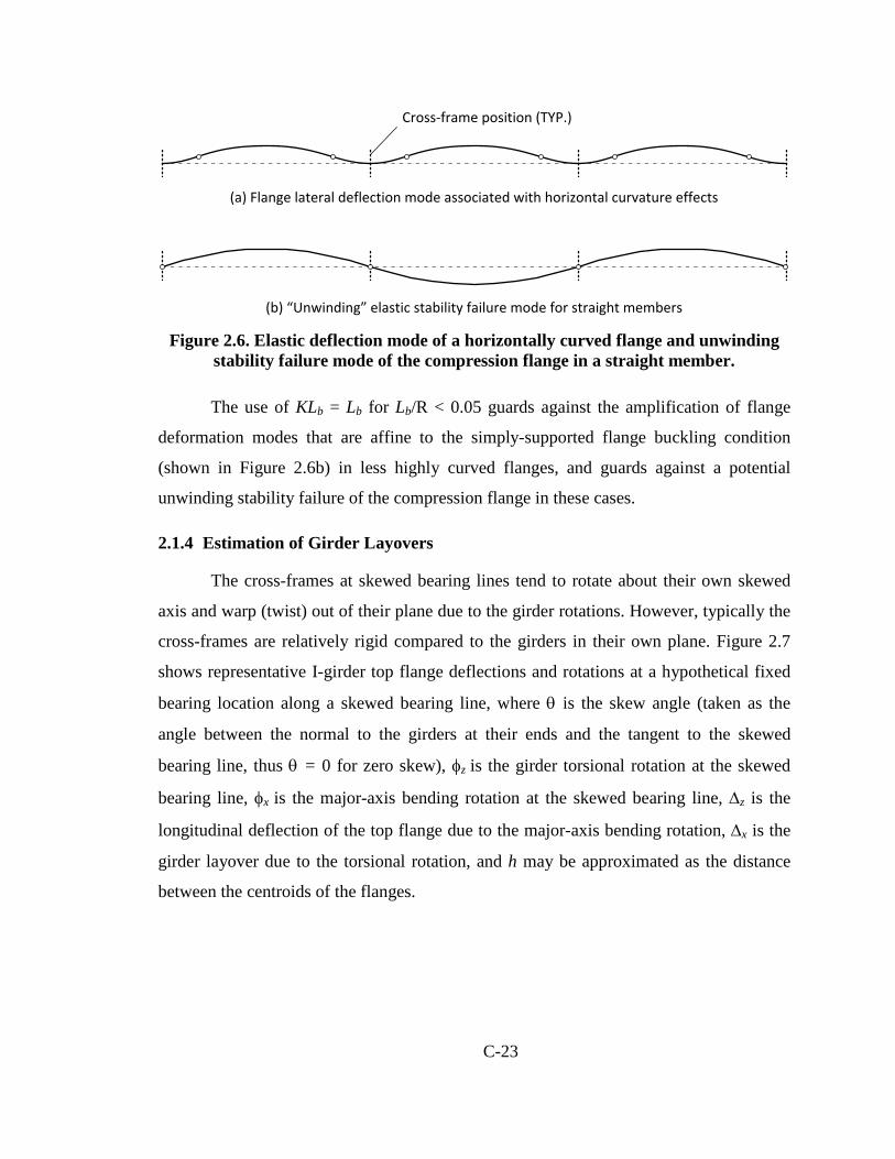
C-23

(a) Flange lateral deflection mode associated with horizontal curvature effects

(b) “Unwinding” elastic stability failure mode for straight members

Cross-frame position (TYP.)

Figure 2.6. Elastic deflection mode of a horizontally curved flange and unwinding

stability failure mode of the compression flange in a straight member.

The use of KLb = Lb for Lb/R < 0.05 guards against the amplification of flange

deformation modes that are affine to the simply-supported flange buckling condition

(shown in Figure 2.6b) in less highly curved flanges, and guards against a potential

unwinding stability failure of the compression flange in these cases.

2.1.4 Estimation of Girder Layovers

The cross-frames at skewed bearing lines tend to rotate about their own skewed

axis and warp (twist) out of their plane due to the girder rotations. However, typically the

cross-frames are relatively rigid compared to the girders in their own plane. Figure 2.7

shows representative I-girder top flange deflections and rotations at a hypothetical fixed

bearing location along a skewed bearing line, where θ is the skew angle (taken as the

angle between the normal to the girders at their ends and the tangent to the skewed

bearing line, thus θ = 0 for zero skew), φz is the girder torsional rotation at the skewed

bearing line, φx is the major-axis bending rotation at the skewed bearing line, ∆z is the

longitudinal deflection of the top flange due to the major-axis bending rotation, ∆x is the

girder layover due to the torsional rotation, and h may be approximated as the distance

between the centroids of the flanges.

C-24

Figure 2.7. Girder top flange deflections and rotations at a fixed bearing location

along a skewed bearing line.

The skewed orientation of the cross-frame forces the major-axis bending rotation

and the torsional rotation of the girder to be coupled at the bearing, based on the

assumption that the in-plane cross-frame deformations are small compared to the

displacements. As shown in Ozgur and White (2007), by assuming small rotations such

that tan(φ) ≅ sin(φ) ≅ φ, the longitudinal deflection of the top flange due to the major-axis

bending rotation can be derived from the geometry as

xφ=∆ hz (2.18)

where φx is measured in radians. Also, the layover of the girders at the skewed bearing

due to the torsional rotations can be expressed as

zφ=∆ hx (2.19)

where φz is measured in radians. Furthermore, because of the kinematic constraint

induced by the in-plane rigidity of the cross-frames, the coupling relationship between

the twist and the major-axis bending rotations is

)θtan(xz φ=φ (2.20)

θ

φx

φz

φ

∆

∆z∆x

θ

h

C-25

Therefore, the layover of the girder at the skewed bearing line (i.e., the lateral

displacement of the top flange relative to the bottom flange) is forced to be

)θtan()θtan(x zx h ∆=φ=∆ (2.21)

to maintain compatibility between the girders and cross-frames.

In the case of a non-fixed bearing, Eq. (2.21) still gives the girder layover at the

bearing, i.e., the relative lateral displacement of the top and bottom flanges. However, the

bottom flange is able to translate based on the degrees of freedom of the bearing.

It is emphasized that properly designed cross-frames often are relatively rigid

compared to the girders in I-girder bridges. Taking advantage of this assumption, also the

layovers of the girders along the spans may be estimated. Figure 2.8 shows representative

girder deflections and rotations for an intermediate cross-frame location where ∆y is the

differential vertical displacement between the girders due to dead loads and s is the girder

spacing.

The layovers within the span can be estimated from the line-girder analysis

vertical displacements, assuming negligible cross-frame in-plane deformations and cross-

frames framed normal to the girders, as (Sanchez, 2011)

∆ = ∆x yh s (2.22)

Figure 2.8 illustrates the definitions of the variables in Eq. (2.22).

Although the above kinematics is illustrated in the context of an I-girder bridge in

this figure, the above equations also can be applied similarly to tub-girders to estimate the

relative lateral displacements between their top and bottom flanges at skewed bearing

lines (Eq. 2.21) and at external intermediate diaphragm locations (Eq. 2.22). In addition,

these results may be divided by the depth h to estimate the girder twist rotations (Eq.

2.20).

The next section takes advantage of these developments to estimate tub-girder

torques.

C-26

Figure 2.8. Magnified girder deflections and rotations at an intermediate cross-frame location.

2.1.5 Estimation of Tub-Girder Torques due to Skew Effects

The effect of skewed supports on the girder torques in tub-girder bridges can be

explained by a few simple mechanistic models. The basic kinematic assumption is the

one discussed in the previous section, i.e., the external diaphragms at the supports are

effectively rigid in their own plane, while they provide relatively little restraint to the tub

girders in their out-of-plane direction. Such assumptions are reasonable approximations

since the external diaphragms are usually solid stiffened plates of relatively small length

compared to the length of the girders, leading to relatively large in-plane stiffness.

Furthermore, the diaphragms are typically I-sections and therefore their torsional stiffness

is relatively small compared to that of the tub girders.

As the girders deflect vertically, they rotate about the line between the bearings at

the supports. Similarly, the diaphragms, acting approximately as rigid plates in their own

plane, rotate about the lines connecting the bearings. When the support line is skewed,

the diaphragm thus forces the girders to twist to maintain compatibility (see Figure 2.9).

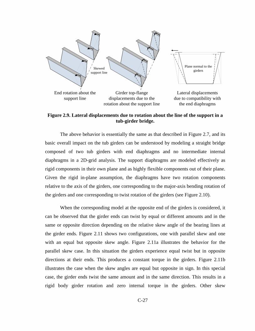
C-27

End rotation about the support line

Lateral displacements due to compatibility with

the end diaphragms

Girder top-flange displacements due to the

rotation about the support line

Plane normal to the girdersSkewed

support line

Figure 2.9. Lateral displacements due to rotation about the line of the support in a tub-girder bridge.

The above behavior is essentially the same as that described in Figure 2.7, and its

basic overall impact on the tub girders can be understood by modeling a straight bridge

composed of two tub girders with end diaphragms and no intermediate internal

diaphragms in a 2D-grid analysis. The support diaphragms are modeled effectively as

rigid components in their own plane and as highly flexible components out of their plane.

Given the rigid in-plane assumption, the diaphragms have two rotation components

relative to the axis of the girders, one corresponding to the major-axis bending rotation of

the girders and one corresponding to twist rotation of the girders (see Figure 2.10).

When the corresponding model at the opposite end of the girders is considered, it

can be observed that the girder ends can twist by equal or different amounts and in the

same or opposite direction depending on the relative skew angle of the bearing lines at

the girder ends. Figure 2.11 shows two configurations, one with parallel skew and one

with an equal but opposite skew angle. Figure 2.11a illustrates the behavior for the

parallel skew case. In this situation the girders experience equal twist but in opposite

directions at their ends. This produces a constant torque in the girders. Figure 2.11b

illustrates the case when the skew angles are equal but opposite in sign. In this special

case, the girder ends twist the same amount and in the same direction. This results in a

rigid body girder rotation and zero internal torque in the girders. Other skew

C-28

configurations would result in unequal twist of the ends resulting in a constant torque

proportional to the relative angle of twist between the girder ends.

Girder G2

Girder G1

Diaphragm rotation constrained by rigid in-plane behavior

Girder twist

Girder major axis bending rotation

Supp

ort D

iaphr

agm

X

Y

Plan view

Figure 2.10. Rigid diaphragm rotation mechanism at a skewed support of a tub-

girder bridge.

Girder G2

Girder G1

X

Y Plan viewSu

ppor

t Di

aphr

agm

Girder G2

Girder G1

Supp

ort

Diap

hrag

m

(a) Parallel skew (b) Equal and opposite skew

Figure 2.11. Girder end rotations in a tub-girder bridge with parallel skew of the

bearing lines and with equal and opposite skew of the bearing lines.

The assumption that the end diaphragms are rigid in their own plane, produces an

upper-bound estimate of the relative angle of twist between the girder ends. This can be

used with a torsional model of the individual girders, in a line-girder analysis, to obtain

an upper-bound estimate of the tub-girder torques due to the skew (Jimenez Chong,

2012).

C-29

As an example application, the above procedure is used to estimate the torsional

moments in the simple-span curved and skewed tub-girder bridge NTSCS29 studied in

NCHRP 12-79 (the bridge name designations are explained in Chapter 4). The bridge is a

twin tub-girder system with a span of L = 225 ft. and a skewed support at its left-hand

end with θ = 15.7°. The bridge framing plan is shown in Figure 2.12.

Figure 2.12. Plan view of NTSCS29.

The girder torsional moments are estimated by multiplying the girder torsional

stiffness GJ/L by the girder twist rotation at the left-hand bearing line φz (since the right-

hand abutment does not have any skew). The girder end twist rotation can be estimated

from the end major-axis bending rotation φx and the support skew angle θ, using Eq.

(2.20). By substituting the simply-supported end major-axis bending rotation, φx =

wL³/(24EI) into Eq. (2.20) and then substituting Eq. (2.20) into the stiffness equation T =

GJφz/L, the upper-bound estimate of the torsional moment due to skew is obtained as T =

wL²GJ tanθ /(24EI), where w is the vertical distributed load, I and J are the bending and

torsional properties of the tub girder and E and G are the material elastic properties. By

using the ratio E/G=2.6, the torsional moment in the simple-span single tub-girder is then

estimated as

θtan2.64

2

IJwLT =

(2.23)

Figure 2.13 illustrates the torsional moments in the exterior girder of bridge

NTSCS29, obtained from the integration of the 3D FEA stresses on the girder cross-

section, as well as the M/R Method estimates with and without the torsional moment T

due to the skew. The results from a 3D FEA model without the two intermediate external

diaphragms shown in Figure 2.12 are also included in the plot. Jimenez Chong (2012)

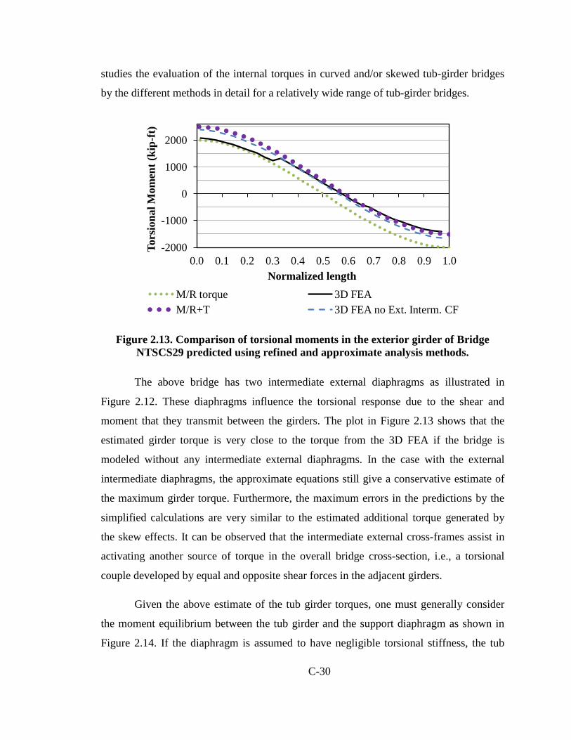
C-30

studies the evaluation of the internal torques in curved and/or skewed tub-girder bridges

by the different methods in detail for a relatively wide range of tub-girder bridges.

Figure 2.13. Comparison of torsional moments in the exterior girder of Bridge NTSCS29 predicted using refined and approximate analysis methods.

The above bridge has two intermediate external diaphragms as illustrated in

Figure 2.12. These diaphragms influence the torsional response due to the shear and

moment that they transmit between the girders. The plot in Figure 2.13 shows that the

estimated girder torque is very close to the torque from the 3D FEA if the bridge is

modeled without any intermediate external diaphragms. In the case with the external

intermediate diaphragms, the approximate equations still give a conservative estimate of

the maximum girder torque. Furthermore, the maximum errors in the predictions by the

simplified calculations are very similar to the estimated additional torque generated by

the skew effects. It can be observed that the intermediate external cross-frames assist in

activating another source of torque in the overall bridge cross-section, i.e., a torsional

couple developed by equal and opposite shear forces in the adjacent girders.

Given the above estimate of the tub girder torques, one must generally consider

the moment equilibrium between the tub girder and the support diaphragm as shown in

Figure 2.14. If the diaphragm is assumed to have negligible torsional stiffness, the tub

-2000

-1000

0

1000

2000

0.0 0.1 0.2 0.3 0.4 0.5 0.6 0.7 0.8 0.9 1.0

Tors

iona

l Mom

ent (

kip-

ft)

Normalized length M/R torque 3D FEA M/R+T 3D FEA no Ext. Interm. CF

C-31

girder torque must be balanced by an internal major-axis bending moment in the tub-

girder, in addition to the moment restraint provided by the in-plane stiffness of the

diaphragm. This in turn influences the overall vertical bending deflections of the tub

girder. This additional effect on the vertical bending deflections typically is neglected in

the above type of hand estimate and the results at this stage are taken as a coarse line-

girder estimate of the tub-girder bridge response.

TT

Mdiaphragm

MdiaphragmMgirder

MgirderJoint

C girderLC

diap

hrag

m

L

Figure 2.14. Idealization of moment equilibrium at the joint between a tub girder

and its support diaphragm.

In bridges that contain intermediate external diaphragms, the behavior is more

complex. External intermediate diaphragms typically are provided to control the specific

differential displacements between the girders that can affect the transverse bending of

the deck and the deck thickness profile (see Figure 2.15). Tub-girder bridges with

external intermediate diaphragms generally require a more refined model than a line-

girder analysis to properly account for the coupling of the tub-girders by the intermediate

diaphragms. However, Helwig et al. suggest an approach that accommodates the use of a

line girder analysis. For simplicity, Helwig et al. (2007) recommend the design of tub-

girder bridges for their final constructed condition assuming no intermediate external

diaphragms or cross-frames. This is followed by the provision of external cross-frames

solely to control the profile of the slab thickness during the placement of the concrete

deck. They give expressions for sizing the external intermediate cross-frames based on

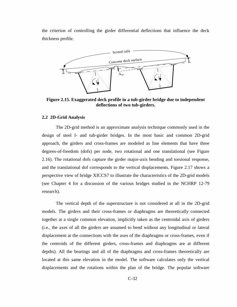
C-32

the criterion of controlling the girder differential deflections that influence the deck

thickness profile.

Figure 2.15. Exaggerated deck profile in a tub-girder bridge due to independent

deflections of two tub-girders.

2.2 2D-Grid Analysis

The 2D-grid method is an approximate analysis technique commonly used in the

design of steel I- and tub-girder bridges. In the most basic and common 2D-grid

approach, the girders and cross-frames are modeled as line elements that have three

degrees-of-freedom (dofs) per node, two rotational and one translational (see Figure

2.16). The rotational dofs capture the girder major-axis bending and torsional response,

and the translational dof corresponds to the vertical displacements. Figure 2.17 shows a

perspective view of bridge XICCS7 to illustrate the characteristics of the 2D-grid models

(see Chapter 4 for a discussion of the various bridges studied in the NCHRP 12-79

research).

The vertical depth of the superstructure is not considered at all in the 2D-grid

models. The girders and their cross-frames or diaphragms are theoretically connected

together at a single common elevation, implicitly taken as the centroidal axis of girders

(i.e., the axes of all the girders are assumed to bend without any longitudinal or lateral

displacement at the connections with the axes of the diaphragms or cross-frames, even if

the centroids of the different girders, cross-frames and diaphragms are at different

depths). All the bearings and all of the diaphragms and cross-frames theoretically are

located at this same elevation in the model. The software calculates only the vertical

displacements and the rotations within the plan of the bridge. The popular software

∆rel

Concrete deck surface

Screed rails

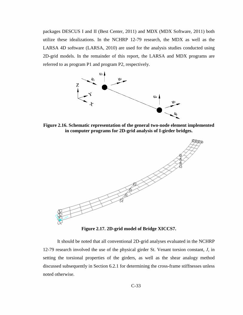
C-33

packages DESCUS I and II (Best Center, 2011) and MDX (MDX Software, 2011) both

utilize these idealizations. In the NCHRP 12-79 research, the MDX as well as the

LARSA 4D software (LARSA, 2010) are used for the analysis studies conducted using

2D-grid models. In the remainder of this report, the LARSA and MDX programs are

referred to as program P1 and program P2, respectively.

Figure 2.16. Schematic representation of the general two-node element implemented

in computer programs for 2D-grid analysis of I-girder bridges.

Figure 2.17. 2D-grid model of Bridge XICCS7.

It should be noted that all conventional 2D-grid analyses evaluated in the NCHRP

12-79 research involved the use of the physical girder St. Venant torsion constant, J, in

setting the torsional properties of the girders, as well as the shear analogy method

discussed subsequently in Section 6.2.1 for determining the cross-frame stiffnesses unless

noted otherwise.

C-34

2.3 2D-Frame Analysis

When using general-purpose software packages, 2D-grid models typically are

constructed using beam or frame elements that have six dofs per node. As shown in

Figure 2.18, these elements have three translational and three rotational dofs at each

node. In this figure, the dofs that are essential to construct a 2D-grid model are u3, u4, u5,

u9, u10, and u11. These implementations are distinguished from the analysis types

discussed in Section 2.2 by referring to them as 2D-frame methods.

Figure 2.18. Schematic representation of the general two-node element implemented in computer programs for 2D-frame analysis of I-girder bridges.

If the structural model is constructed all in one plane, with no depth information

being represented, and if the element formulations do not include any coupling between

the conventional 2D-grid dofs and the additional dofs (which is practically always the

case), 2D-frame models actually do not provide any additional information beyond the

ordinary 2D-grid solutions. Assuming gravity loading normal to the plane of the

structure, all the displacements at the three additional nodal dofs will be zero. Therefore,

for purposes of discussion in this report, 2D-frame models are also referred to as 2D-

grid. Nevertheless, the 2D-grid implementation in LARSA 4D discussed in this report is

specifically a 2D-frame model.

C-35

2.4 Plate and Eccentric Beam Analysis

The MDX Software system implements a second type of model for the analysis of

I- and tub-girder bridges that is commonly referred to as a plate and eccentric beam

model. In this idealization, the composite bridge deck is modeled using flat shell (or

plate) finite elements and the girders are modeled using 6 dof per node frame elements

(total of 12 dofs per element, see Figure 2.18) with an offset relative to the slab (see

Figure 2.19).

The plate and eccentric beam model is used typically for analysis of composite

bridge structures in their final constructed configuration. In the NCHRP 12-79 research,

this type of modeling approach was used in the design of various parametric study

bridges. Specifically, it was used for the design analysis of the bridges in their final

constructed condition. The reader is referred to Chapter 4 for an overview of the various

bridges considered in the NCHRP research.

Figure 2.19. Schematic representation of the plate-and-eccentric-beam model.

2.5 Conventional 3D-Frame Analysis

An analysis model may be referred to as a conventional 3D-frame if:

• The structure is modeled using the above 3D frame elements and the centroid and

shear center of the girders are modeled at their actual spatial locations,

• The actual location of the cross-frames or diaphragms through the depth is

modeled (typically using a single frame element to represent each entire cross-

frame or diaphragm between the points of connection to the other components)

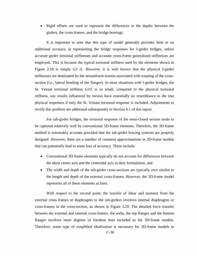
C-36

• Rigid offsets are used to represent the differences in the depths between the

girders, the cross-frames, and the bridge bearings.

It is important to note that this type of model generally provides little to no

additional accuracy in representing the bridge responses for I-girder bridges, unless

accurate girder torsional stiffnesses and accurate cross-frame generalized stiffnesses are

employed. This is because the typical torsional stiffness used by the elements shown in

Figure 2.18 is simply GJ /L. However, it is well known that the physical I-girder

stiffnesses are dominated by the nonuniform torsion associated with warping of the cross-

section (i.e., lateral bending of the flanges). In most situations with I-girder bridges, the

St. Venant torsional stiffness GJ/L is so small, compared to the physical torsional

stiffness, any results influenced by torsion have essentially no resemblance to the true

physical responses if only the St. Venant torsional response is included. Adjustments to

rectify this problem are addressed subsequently in Section 6.1 of this report.

For tub-girder bridges, the torsional response of the semi-closed section tends to

be captured relatively well by conventional 3D-frame elements. Therefore, the 3D-frame

method is reasonably accurate provided that the tub-girder bracing systems are properly

designed. However, there are a number of common approximations in 3D-frame models

that can potentially lead to some loss of accuracy. These include:

• Conventional 3D-frame elements typically do not account for differences between

the shear center axis and the centroidal axis in their formulation, and

• The width and depth of the tub-girder cross-sections are typically very similar to

the length and depth of the external cross-frames. However, the 3D-frame model

represents all of these elements as lines.

With respect to the second point, the transfer of shear and moment from the

external cross-frames or diaphragms to the tub-girders involves internal diaphragms or

cross-frames in the cross-section, as shown in Figure 2.20. The detailed force transfer

between the external and internal cross-frames, the webs, the top flanges and the bottom

flanges involves more degrees of freedom than included in the 3D-frame models.

Therefore, some type of simplified idealization is necessary for 3D-frame models to

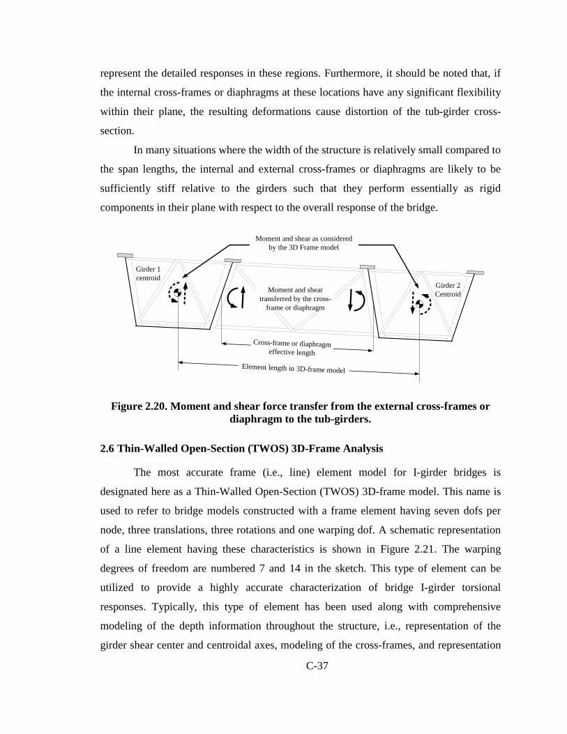
C-37

represent the detailed responses in these regions. Furthermore, it should be noted that, if

the internal cross-frames or diaphragms at these locations have any significant flexibility

within their plane, the resulting deformations cause distortion of the tub-girder cross-

section.

In many situations where the width of the structure is relatively small compared to

the span lengths, the internal and external cross-frames or diaphragms are likely to be

sufficiently stiff relative to the girders such that they perform essentially as rigid

components in their plane with respect to the overall response of the bridge.

Girder 2Centroid

Girder 1centroid

Cross-frame or diaphragm effective length

Moment and shear transferred by the cross-

frame or diaphragm

Moment and shear as considered by the 3D Frame model

Element length in 3D-frame model

Figure 2.20. Moment and shear force transfer from the external cross-frames or diaphragm to the tub-girders.

2.6 Thin-Walled Open-Section (TWOS) 3D-Frame Analysis

The most accurate frame (i.e., line) element model for I-girder bridges is

designated here as a Thin-Walled Open-Section (TWOS) 3D-frame model. This name is

used to refer to bridge models constructed with a frame element having seven dofs per

node, three translations, three rotations and one warping dof. A schematic representation

of a line element having these characteristics is shown in Figure 2.21. The warping

degrees of freedom are numbered 7 and 14 in the sketch. This type of element can be

utilized to provide a highly accurate characterization of bridge I-girder torsional

responses. Typically, this type of element has been used along with comprehensive

modeling of the depth information throughout the structure, i.e., representation of the

girder shear center and centroidal axes, modeling of the cross-frames, and representation

C-38

of bearings all at their corresponding depths (Chang, 2006; Huang, 1996). Selected

studies have been conducted in the NCHRP 12-79 research using this type of element as

implemented by Chang (2006) in the program GT-Sabre. GT-Sabre not only includes a

refined open-section thin-walled beam theory representation of the I-girders, but it also

includes the modeling of all the individual cross-frame components (i.e., the separate

modeling of the cross-frame chords and diagonals using individual frame elements). In

GT-Sabre, the individual elements representing the cross-frame members are tied to the

girder nodes by rigid offsets.

The TWOS 3D-frame modeling approach is capable of matching the results of 3D

FEA quite closely, with the exception that it is not able to capture the influence of I-

girder web distortion on the physical responses. Web distortion can be an important

factor when modeling composite I-girder torsional responses (Chang, 2006; Chang and

White, 2008), but otherwise, its effect is typically inconsequential. In basic terms, if a

TWOS element is tied to a slab via a rigid link, similar to the plate and eccentric beam

modeling approach, the slab will incorrectly restrain the lateral bending of the bottom

flange unless special modeling procedures, such as those discussed by Chang (2006), are

invoked.

Figure 2.21. Schematic representation of a general two-node 3D TWOS frame

element implemented in computer programs of I-girder bridges.

C-39

As discussed by Chang (2006), there are a number of other complexities that are

difficult to handle in the implementation of 3D TWOS frame elements. These include the

modeling of continuity conditions at cross-section transitions (e.g., changes in flange

thickness and/or width), and the modeling of the continuity conditions for bifurcated

girders (three girder elements framing into a common node). In addition, GT-Sabre

(Chang, 2006) is the only known software that correctly displays the detailed three-

dimensional deformed geometry from a TWOS 3D-frame analysis. Most TWOS 3D-

frame elements have been implemented only in a structural engineering research setting,

and either do not include any capability for graphical display of the deflected geometry at

all, or display the deformed geometry only as the deformed centroidal axis of the

member. Although advanced simulation software systems such as ABAQUS (Simulia,

2010), typically can graphically render the 3D I-section geometry, they do not graphically

display the detailed warping deformations of 3D TWOS frame elements when they

render the displaced geometry of the structure. As a result of the above complexities, as

well as the fact that with increasing computer speeds, large degree of freedom 3D FEA

computations can be conducted in a small amount of time, 3D FEA generally is preferred

over TWOS 3D-frame analysis for design of steel girder bridges when line-girder or 2D-

grid methods do not suffice.

2.7 Calculation of Component Forces Given the Line-Girder or 2D-Grid Analysis Results for Tub-Girder Bridges

Due to the idealization of the tub-girders, cross-frames and diaphragms as “line”

elements in the above line-girder, 2D-grid, or 3D-frame approaches, the analysis of tub-

girder bridges by any of these methods requires additional calculations to estimate the

forces in the bracing components, as well as the stresses in the tub-girders. The bracing

components include the top horizontal truss, also known as the top flange lateral bracing

(TFLB) system, and the different components of the internal and external cross-frames

and diaphragms at intermediate locations and at the supports.

To ensure good accuracy in the evaluation of the component forces in curved and

skewed tub-girder bridges, the overall analysis must accurately capture the effects of

curvature and skew. In general, conventional line-girder analysis calculations do not

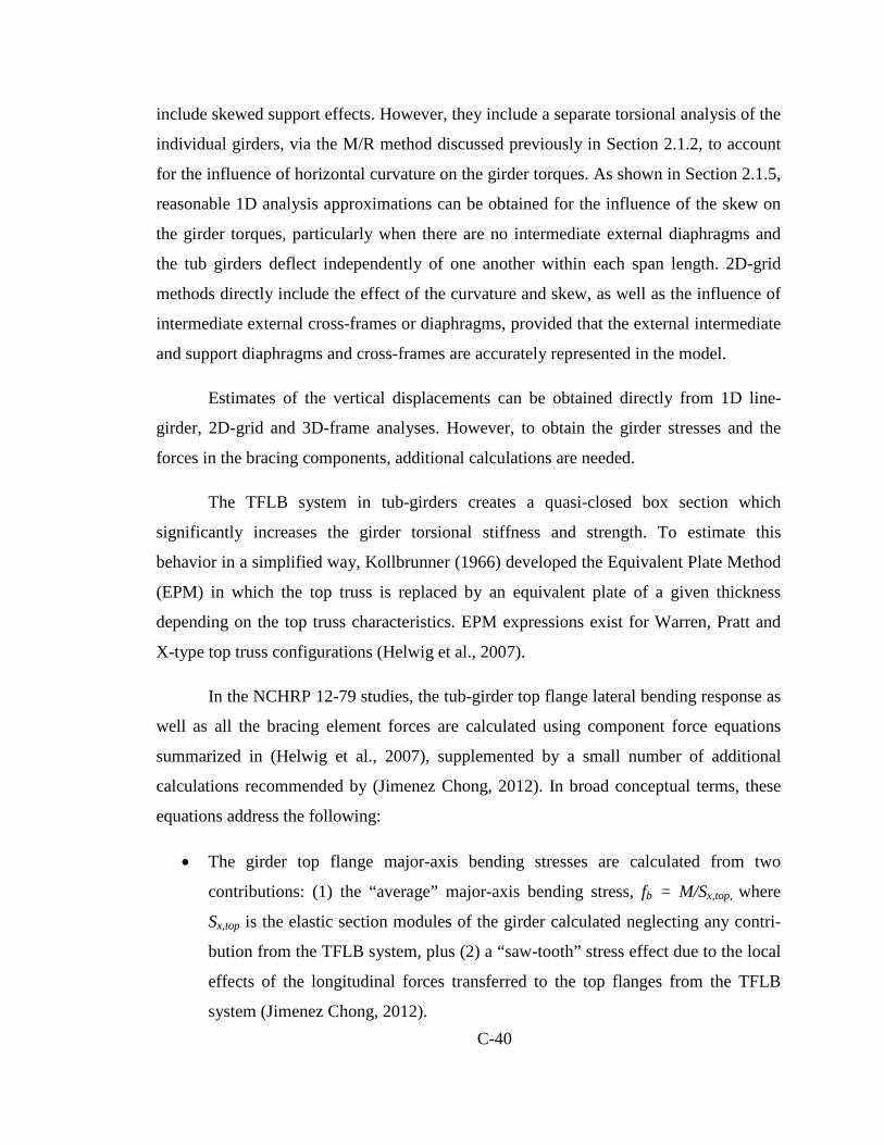
C-40

include skewed support effects. However, they include a separate torsional analysis of the

individual girders, via the M/R method discussed previously in Section 2.1.2, to account

for the influence of horizontal curvature on the girder torques. As shown in Section 2.1.5,

reasonable 1D analysis approximations can be obtained for the influence of the skew on

the girder torques, particularly when there are no intermediate external diaphragms and

the tub girders deflect independently of one another within each span length. 2D-grid

methods directly include the effect of the curvature and skew, as well as the influence of

intermediate external cross-frames or diaphragms, provided that the external intermediate

and support diaphragms and cross-frames are accurately represented in the model.

Estimates of the vertical displacements can be obtained directly from 1D line-

girder, 2D-grid and 3D-frame analyses. However, to obtain the girder stresses and the

forces in the bracing components, additional calculations are needed.

The TFLB system in tub-girders creates a quasi-closed box section which

significantly increases the girder torsional stiffness and strength. To estimate this

behavior in a simplified way, Kollbrunner (1966) developed the Equivalent Plate Method

(EPM) in which the top truss is replaced by an equivalent plate of a given thickness

depending on the top truss characteristics. EPM expressions exist for Warren, Pratt and

X-type top truss configurations (Helwig et al., 2007).

In the NCHRP 12-79 studies, the tub-girder top flange lateral bending response as

well as all the bracing element forces are calculated using component force equations

summarized in (Helwig et al., 2007), supplemented by a small number of additional

calculations recommended by (Jimenez Chong, 2012). In broad conceptual terms, these

equations address the following:

• The girder top flange major-axis bending stresses are calculated from two

contributions: (1) the “average” major-axis bending stress, fb = M/Sx,top, where

Sx,top is the elastic section modules of the girder calculated neglecting any contri-

bution from the TFLB system, plus (2) a “saw-tooth” stress effect due to the local

effects of the longitudinal forces transferred to the top flanges from the TFLB

system (Jimenez Chong, 2012).

C-41

• The TFLB diagonal forces, Dtot, are determined from the girder torques and the

girder major-axis bending moments as the sum of two contributions, DEPM and

DBend. The contribution DEPM is obtained from a girder pseudo closed-section

torsional analysis, and the contribution DBend is obtained by considering the axial

deformations of the girder top flanges due to flexure and the continuity of the

TFLB struts and diagonals with the top flanges.

• The TFLB transverse strut force Stot is obtained from two contributions: (1) the

force SBend required to equilibrate the lateral component of the diagonal forces at

the joints of the TFLB system, and (2) the force SLat caused by the lateral compo-

nent of the transverse normal forces in the sloping webs required to resist the

distributed vertical loads applied to the top flanges of the tub girder.

• The lateral bending stresses in the tub-girder top flanges, f Tot, are calculated

generally from three effects: (1) the effect of the lateral forces SBend coming from

the TFLB struts, f Bend (this effect is zero for X-type TFLB systems, but is non-

zero due to the “back-and-forth” loading effects on the flanges from the

deformations of the top flange truss in Warren-type TFLB systems), (2) the effect

of the lateral component of the transverse normal forces in the tub-girder sloping

webs required to resist the distributed vertical loads applied to the girder top

flanges, f p, and (3) the influence of the horizontal curvature of the top flanges

f M/Rh from Eq. (2.15). In addition, the influence of overhang bracket loads per

Eqs. (2.13) and (2.14) is included on the outside flanges of fascia girders.

• The forces in the internal cross-frame diagonals D and the forces in the internal

cross-frame top chords S are obtained from tub-girder cross-section distortional

force equations developed by (Fan and Helwig, 2002). These forces depend upon

the spacing between the internal cross-frames measured along the girder length,

sK, and they are driven by the effects from the equivalent distributed torque M/R

associated with the horizontal curvature as well as an eccentricity effect of the

vertical loads w, which are assumed to be applied to the top flanges.

• The forces in the intermediate external cross-frame diagonals FD, the top chord,

FT, and the bottom chord, FB, are determined based on the spacing between the

C-42

external cross-frames along the length of the bridge, as well as the exterior and

interior girder rotations and vertical displacements at the external cross-frame

locations, obtained from an analysis neglecting the intermediate external cross-

frames. These equations were developed by Li (2004) specifically to control the

relative deformations shown in Figure 2.15 for two-girder systems.

Jimenez Chong (2012) provides a detailed overview of the background and development

of the various component force equations. The following sections document all the

specific component force calculations utilized in the NCHRP 12-79 studies. Section 2.7.8

provides a definition of all the variables used in the equations.

2.7.1 Input

2.7.1.1 Major-Axis Bending Moment, M

The girder major-axis bending moment distribution is directly obtained from a 1D

or 2D analysis.

2.7.1.2 Torque, T

The girder torsional moment is directly obtained from a 2D-grid analysis. With a

1D line-girder analysis, the torsional moment distribution is calculated independently for

each girder and each span as follows. At a location s, the torsional moment due to

curvature is given by:

( ) ( )C0 0

1 L M sT L s ds

L R= −∫ (2.24)

( ) ( )C0 0

s

C

M sT s T ds

R= − ∫ (2.25)

Concentrated torques are applied to the girders from the skewed supports. The girder

internal torque from the skew in each span is obtained by determining a twist rotation at

each end of the span (ends 1 and 2) and then multiplying the total relative twist between

the two ends by the St. Venant torsional stiffness GJ/L. The resulting constant torque in a

given span due to skewed supports is given by:

C-43

1 221( tan tan )S y yGT JL

φ φ= − θ + θ (2.26)

The total torque is equal to the sum of the torque due to curvature and due to skew:

( ) ( )C ST s T s T= + (2.27)

2.7.1.3 Average Major-Axis Bending Stress

The top flange “average” major-axis bending stress is calculated as

,b

x top

MfS

= (2.28)

where Sx,top does not include any contribution from the TFLB system.

2.7.1.4 Vertical Displacements, ∆

The vertical displacements are directly obtained from the 1D or 2D analysis.

2.7.1.5 Girder Twist Rotations, φ

The girder twist rotations for 2D analysis are directly obtained from the analysis.

For 1D analysis the twist rotations are estimated as follows. At a location s, the twist

rotation due to curvature is given by:

( ) ( ),1 1x C

EIs sR GJ

φ = + ∆ (2.29)

The twist rotation due to skew is calculated at each support by the equation

( )tanxi yi iφ = −φ θ (2.30)

and the distribution along the span length is assumed to vary linearly as

( ), 1 1 2( )x S x x xssL

φ = φ − φ − φ (2.31)

The total girder twist rotations are equal to the sum of those due to curvature and those

due to skew:

C-44

( ) ( ) ( ), ,x x C x Ss s sφ = φ + φ (2.32)

2.7.2 Equivalent Plate Method

The Equivalent Plate Method allows the estimation of the girder torsional

constant as

204

i ii

AJb t

=∑

(2.33)

The top truss contribution to the system torsional behavior is estimated by replacing the

truss by a fictitious equivalent plate. The equivalent plate thickness t* can be determined

for different truss layouts and cross-sectional areas of the diagonals and struts.

2.7.3 Warren TFLB Systems

The following sketch illustrates the general layout of a Warren TFLB System.

s

a dα

Figure 2.22. Warren TFLB system.

2.7.3.1 Equivalent Plate Thickness

The equivalent plate thickness for a Warren TFLB system is calculated using

3 3*

23d f

E satG d s

A A

=

+ (2.34)

2.7.3.2 TFLB Diagonal Forces

The separate contributions to the TFLB diagonal forces in a Warren TFLB system

are determined as follows.

C-45

Torsion contribution

02TqA

= (2.35)

sinTorsionqaD =

α (2.36)

Bending contribution 2

2 21 2sin sin

2d s f f

d a sKA A b t

= + α + α (2.37)

1

cosbBend

f sDK

α=

(2.38)

Other contributions

The lateral components of the transverse forces in the inclined girder webs are assumed

to be developed entirely by the TFLB struts.

The influence of distortion on the TFLB diagonal forces is assumed to be negligible.

Total TFLB diagonal forces

Tot Torsion BendD D D= + (2.39)

2.7.3.3 TFLB Strut Forces

The transverse strut forces in a Warren TFLB system are determined using the

following equations.


, ,sin sinTorsion Tot i i Tot j jS D D= α + α (2.40)

This is typically neglected, and is not considered in the base calculations employed in the

NCHRP 12-79 research.

Bending contribution

sinBend BendS D= − α (2.41)

C-46

Transverse load contribution

tan2wp = φ

(2.42)

LatS ps= (2.43)

Girder distortional contribution

04K

Dists b b MS ew

A a R = ± − (2.44)

SDist affects only the struts that also serve as internal cross-frame top chords.

The only significant girder distortions are assumed to be due to eccentricity of the vertical

load w, and due to the horizontal curvature effects.

Other contributions

At external cross-frame locations, significant TFLB strut forces may be developed. These

forces should be estimated by basic principles considering the overall force paths and

joint equilibrium for the bracing components.

Total TFLB strut forces

Tot Bend Lat Torsion DistS S S S S= + + + (2.45)

2.7.3.4 Intermediate Internal Cross-Frame Diagonals

Distortion effects due to eccentric vertical load and due to horizontal curvature are

assumed to be the only contributor to the internal cross-frame diagonal forces,

02K DKs L M bD ew

A R a = ± − (2.46)

2.7.3.5 Top Flange Lateral Bending

The tub-girder top flange lateral bending stresses are determined using the


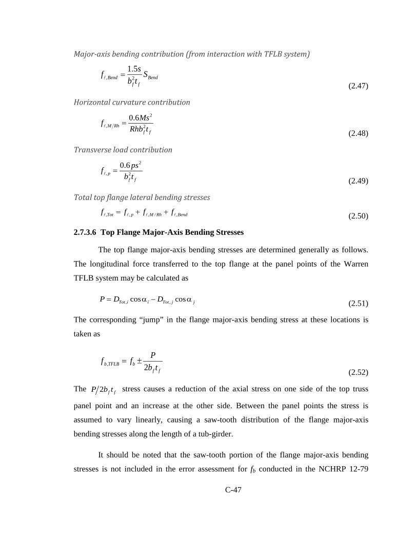
C-47

Major-axis bending contribution (from interaction with TFLB system)

, 2

1.5Bend Bend

f f

sf Sb t

=

(2.47)

Horizontal curvature contribution 2

, 2

0.6M Rh

f f

MsfRhb t

=

(2.48)

Transverse load contribution 2

, 2

0.6p

f f

psfb t

=

(2.49)

Total top flange lateral bending stresses

, , , / ,Tot p M Rh Bendf f f f= + + (2.50)

2.7.3.6 Top Flange Major-Axis Bending Stresses

The top flange major-axis bending stresses are determined generally as follows.

The longitudinal force transferred to the top flange at the panel points of the Warren

TFLB system may be calculated as

, ,cos cosTot i i Tot j jP D D= α − α (2.51)

The corresponding “jump” in the flange major-axis bending stress at these locations is

taken as

, 2b TFLB bf f

Pf fb t

= ± (2.52)

The 2 f fP b t stress causes a reduction of the axial stress on one side of the top truss

panel point and an increase at the other side. Between the panel points the stress is

assumed to vary linearly, causing a saw-tooth distribution of the flange major-axis

bending stresses along the length of a tub-girder.

It should be noted that the saw-tooth portion of the flange major-axis bending

stresses is not included in the error assessment for fb conducted in the NCHRP 12-79

C-48

research. This is because conventional software, such as MDX, does not include this

contribution to the major-axis bending stress in its calculations.

2.7.4 X-Type TFLB Systems

The following sketch shows the general configuration of an X-type TFLB system

Figure 2.23. X-type TFLB system.


The equivalent plate thickness for an X-type TFLB system is calculated using

3 3*

2 6d f

E satG d s

A A

=

+ (2.53)


The separate contributions to the TFLB diagonal forces in an X-type TFLB

system are determined as follows.


02TqA

= (2.54)

2sinTorsionqaD =

α (2.55)


22

2 sind s

d aKA A

= + α (2.56)

2

cosbBend

f sDK

α=

(2.57)

C-49

Other contributions




Total TFLB Diagonal Forces



The transverse strut forces in a Warren TFLB system are determined using the



, ,sin sinTorsion Tot i i Tot j jS D D= α + α (2.59)

This is typically neglected, and is not considered in the base calculations.


2 sinBend BendS D= − α (2.60)


tan2wp = φ

(2.61)

LatS ps= (2.62)


04K

Dists b b MS ew

A a R = ± − (2.63)

SDist is assumed to affect the struts that also serve as internal cross-frame top chords.



C-50

Other contributions


forces should be estimated by basic principles considering the overall force paths and

joint equilibrium for the bracing components.

Total


2.7.4.4 Intermediate Internal Cross-Frame Diagonal Forces


assumed to be the only contributor to the internal cross-frame diagonal forces.

02K DKs L M bD ew

A R a = ± − (2.65)


The tub-girder top flange lateral bending stresses in X-type TFLB systems are

determined using the following equations.

Major-axis bending contribution (from interaction with TFLB system)

, 0Bendf = (2.66)


, 2

0.6M Rh

f f

MsfRhb t

=

(2.67)

Transverse load contribution: 2

, 2

0.6p

f f

psfb t

=

(2.68)

Total


C-51



The longitudinal force transferred to the top flange at the panel points of the X-type


, ,cos cosTot i i Tot j jP D D= α − α (2.70)

The corresponding “jump” in the flange major-axis bending stress at these locations is

taken as

, 2b TFLB bf f

Pf fb t

= ± (2.71)

The 2 f fP b t stress causes a reduction of the axial stress at one side of the top truss work

point and an increase at the other side. Between the work points, the stress is assumed to

vary linearly causing a saw-tooth distribution of the flange major-axis bending stresses

along the length of a tub-girder.

It should be noted that the saw-tooth portion of the flange major-axis bending

stresses is not included in the error assessment for fb conducted in the NCHRP 12-79

research. This is because conventional software, such as MDX, does not include this

contribution to the major-axis bending stress in its calculations.

2.7.5 Pratt TFLB Systems

The following sketch illustrates the general layout of a Pratt TFLB System.

Figure 2.24. Pratt TFLB system.


The equivalent plate thickness for a Pratt TFLB system is calculated using

C-52

3 3*

2 6d f

E satG d s

A A

=

+ (2.72)


The separate contributions to the TFLB diagonal forces in a Pratt TFLB system

are determined as follows.


02TqA

= (2.73)

sinTorsionqaD =

α (2.74)

Bending contribution 2

2 21 2sin sin

2d s f f

d a sKA A b t

= + α + α (2.75)

1

cosbBend

f sDK

α=

(2.76)

Other contributions




Total



The transverse strut forces in a Pratt TFLB system are determined using the


C-53


TorsionS qa= (2.78)


sinBend BendS D= − α (2.79)


tan2wp = φ

(2.80)

LatS ps= (2.81)


04K

Dists b b MS ew

A a R = ± − (2.82)

SDist is assumed to affect the struts that also serve as internal cross-frame top chords.



Other contributions


forces are not considered in the base calculations.

Total


2.7.5.4 Intermediate Internal Cross-Frame Diagonals


assumed to be the only contributor to the internal cross-frame diagonal forces.

02K DKs L M bD ew

A R a = ± − (2.84)

C-54


The tub-girder top flange lateral bending stresses in Pratt TFLB systems are

determined using the following equations.

Major-axis bending contribution (from interaction with TFLB system):

, 2

1.5Bend Bend

f f

sf Sb t

=

(2.85)


, 2

0.6M Rh

f f

MsfRhb t

=

(2.86)

Transverse load contribution 2

, 2

0.6p

f f

psfb t

=

(2.87)

Total




The longitudinal force transferred to the top flange at the panel points of the X-type


cosPratt TotP D= α (2.89)

Pr, 2

attb TFLB b

f f

Pf fb t

= ± (2.90)

The Pr 2att f fP b t stress causes a reduction of the axial stress at one side of the top truss

work point and an increase at the other side. Between the work points, the stress is

assumed to vary linearly causing a saw-tooth stress distribution of the flange major-axis

bending stresses along the length of a tub-girder.

C-55

2.7.6 External Intermediate Cross-Frame Forces

The forces in the diagonals of external intermediate cross-frames are calculated

using the equation

( ), ,int 1 ,

2

4 i w ext e w e w relD

e

L L KF GJ

Kφ + φ − ∆

= (2.91)

whereas the forces in the top and bottom chords are obtained using

( ) ( )( )

, ,int4 w ext w D K e iT

k i e

GJ F L L LF

h L Lφ − φ − −

=+ (2.92)

cosB D TF F F= ± ψ − (2.93)

where the variables in these equations are

cos sinK K TL h L= ψ + ψ (2.94)

00 1 1 1 cos

2eEIKGJ

β = + + − (2.95)

1i e

eL LKa c

+=

+ (2.96)

( )3 3

2 0 1 sin 212

i ee e e i e K

L LK K K L L LEI GJ

+= ψ +

(2.97)

2.7.7 Support Diaphragms

The following equations from Helwig et al. (2007) are used for as a basic strength

and stiffness criterion for the support diaphragms in the NCHRP 12-79 project research.

Strength requirement

( )1 2

, 0.58d strengthd y

T TAL F

+=

(2.98)

Stiffness requirement

( ) 2r fx a b= + (2.99)

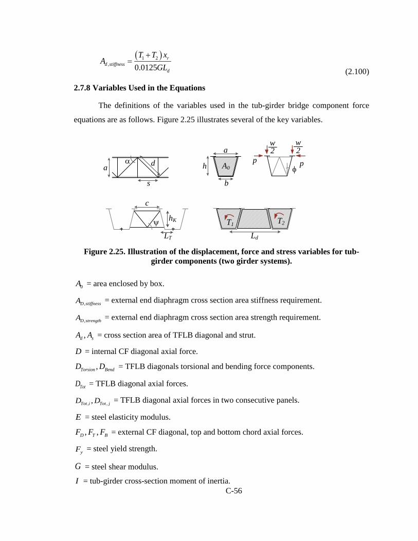
C-56

( )1 2, 0.0125

rd stiffness

d

T T xA

GL+

= (2.100)

2.7.8 Variables Used in the Equations

The definitions of the variables used in the tub-girder bridge component force

equations are as follows. Figure 2.25 illustrates several of the key variables.

a

s

dα

a

b

A0

w2

w2

p pφh

hK

c

LT

ψ

Ld

T1 T2

Figure 2.25. Illustration of the displacement, force and stress variables for tub-

girder components (two girder systems).

0A = area enclosed by box.

,D stiffnessA = external end diaphragm cross section area stiffness requirement.

,D strengthA = external end diaphragm cross section area strength requirement.

,d sA A = cross section area of TFLB diagonal and strut.

D = internal CF diagonal axial force.

,Torsion BendD D = TFLB diagonals torsional and bending force components.

TotD = TFLB diagonal axial forces.

, ,,Tot i Tot jD D = TFLB diagonal axial forces in two consecutive panels.

E = steel elasticity modulus.

, ,D T BF F F = external CF diagonal, top and bottom chord axial forces.

yF = steel yield strength.

G = steel shear modulus.

I = tub-girder cross-section moment of inertia.

C-57

J = St Venant tub-girder torsional constant.

1 2,K K = EPM constants for TFLB force calculation.

0 1 2, ,e e eK K K = constants for external intermediate CF force calculation.

dL = diaphragm length between supports.

DKL = length of internal CF diagonal.

, i eL L = internal and external girder CL lengths.

KL = constant for external intermediate CF force calculation.

TL = external CF top chord distance to tub centerline.

M = girder bending moment.

R = radius of horizontal curvature of girder.

, , ,DistLat Be To ind rs onS S S S = TFLB struts lateral, bending, distortional and torsion force

components.

TotS = TFLB strut axial forces.

,x topS = top flange section modulus.

T = total girder torsional moment

,C ST T = girder torsional moments due to curvature and skew.

1 2,T T = girder end torques.

a = box girder top width.

b = bottom flange width.

fb = top flange width.

c = external CF top chord length.

d = TFLB diagonal length.

e = effective eccentricity of resultant distributed load.

bf = average top flange major-axis bending stress.

,b TFLBf = top flange major-axis bending stress including the TFLB interaction.

, ,,Bend pf f = lateral force and major-axis bending components of lateral bending.

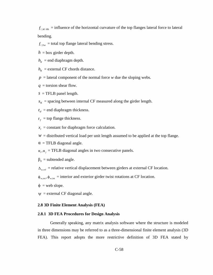
C-58

, /M Rhf = influence of the horizontal curvature of the top flanges lateral force to lateral

bending.

,Totf = total top flange lateral bending stress.

h = box girder depth.

dh = end diaphragm depth.

Kh = external CF chords distance.

p = lateral component of the normal force w due the sloping webs.

q = torsion shear flow.

s = TFLB panel length.

Ks = spacing between internal CF measured along the girder length.

dt = end diaphragm thickness.

ft = top flange thickness.

rx = constant for diaphragm force calculation.

w = distributed vertical load per unit length assumed to be applied at the top flange.

α = TFLB diagonal angle.

α ,αi j = TFLB diagonal angles in two consecutive panels.

0β = subtended angle.

,w rel∆ = relative vertical displacement between girders at external CF location.

, ,int,w ext wφ φ = interior and exterior girder twist rotations at CF location.

φ = web slope.

ψ = external CF diagonal angle.

2.8 3D Finite Element Analysis (FEA)

2.8.1 3D FEA Procedures for Design Analysis

Generally speaking, any matrix analysis software where the structure is modeled

in three dimensions may be referred to as a three-dimensional finite element analysis (3D

FEA). This report adopts the more restrictive definition of 3D FEA stated by

C-59

AASHTO/NSBA G13.1 (2011). According to G13.1, an analysis method is classified as a

3D FEA if:

1) The superstructure is modeled fully in three dimensions,

2) The individual girder flanges are modeled using beam, shell or solid type

elements,

3) The girder webs are modeled using shell or solid type elements,

4) The cross-frames or diaphragms are modeled using truss, beam, shell or solid type

elements as appropriate, and

5) The concrete deck is modeled using shell or solid elements (when considering the

response of the composite structure).

It is important to recognize that the finite element method generally entails the use

of a large number “elements” that are small in dimension compared to the structural

dimensions that influence the responses to be evaluated. Furthermore, there are many

detailed decisions that either explicitly or implicitly can impact the results, and therefore

it is important to recognize that not all 3D FEA models are the same. When creating a 3D

FEA model, the engineer (explicitly, or implicitly) selects a theoretical representation for

the various parts of the structure (e.g., 3D solid, thick shell, thin shell, Timoshenko beam,

Euler-Bernoulli beam, etc.), a mesh density sufficient to ensure convergence of the FEA

numerical approximations within an acceptable tolerance, an element formulation type

such as a displacement-based, flexibility-based or mixed formulation, an interpolation

order for the different element response quantities (e.g., linear or quadratic order

interpolation of the element internal displacements), a numerical integration scheme for

evaluation of the element nodal forces and stiffnesses (e.g., standard Gauss quadrature,

Gauss-Lobatto integration, etc.), and procedures for calculating, extrapolating, and

smoothing or averaging of element internal stresses and strains.

The handling of the above attributes, as well as various other important analytical

and numerical considerations, is beyond the scope of this document. However, with the

exception of the first two of the above considerations, these decisions are more within the

realm of finite element software development rather than the domain of engineering

C-60

design and analysis. The engineer generally should understand the broad aspects of the

assumptions and limitations of the 3D FEA procedures, to ensure their proper application.

Furthermore, generally he or she should conduct testing and validation studies with the

software to ensure that the methods work as intended and that they provide correct

answers for relevant benchmark problems.

Different analysis objectives, although they may be applied to the same structure,

generally require different finite element models. For example, 3D FEA can be very

useful for performing refined local stress analysis of complex structural details. This is

not the objective within the context of this report. The recommendations in this report

address the calculation of accurate:

• Elastic girder vertical deflections, lateral deflections, and rotations,

• Elastic girder major-axis bending stresses, or the corresponding bending

moments, flange lateral bending stresses, web shear forces, and for tub girders,

bottom flange shear stresses,

• Elastic cross-frame component axial forces,

• Elastic diaphragm major-axis bending stresses and web shear stresses, or the

corresponding bending moments, and web shear forces, and

• Where composite action is considered, elastic slab normal and shear stresses and

strains.

Basically, the objective of the 3D FEA models targeted in this report is the

accurate calculation of all the bridge responses utilized by the AASHTO LRFD Speci-

fications for the overall design of curved and/or skewed steel I- and tub-girder bridge

structures.

There are various 3D FEA modeling strategies that can accomplish this objective.

The approach recommended by the NCHRP 12-79 research, and utilized by the project

team for their three-dimensional elastic finite element design analyses (i.e., 3D FEA

analyses conducted for the purpose of design or design checking) entails the use of:

C-61

• A general-purpose 4-node quadrilateral Reissner-Mindin (shear-deformable) shell

element for modeling I- and tub-girder webs, tub-girder bottom flanges, and the

concrete deck slab, as well as a compatible 3-node triangular shell element, used

sparingly for modeling of the concrete deck at skewed bearing lines (tub-girder

webs and bottom flanges are modeled at skewed bearing lines by “fanning” the

geometry of the quadrilateral elements).

• A compatible 2-node shear-deformable beam element for modeling I-girder

flanges, tub-girder top flanges, bearing stiffeners, connection plates, intermediate

transverse stiffeners, longitudinal stiffeners, and the “lips” of tub-girder bottom

flanges extending outside of the webs.

• A 2-node shear-deformable beam element for modeling of cross-frame chords.

The cross-frame chords are modeled at their physical location through the depth

of the structure. Their connections into the girders are modeled generally using

multi-point constraints so that the FEA discretization through the depth of the

webs does not have to be adjusted to place nodes at the specific cross-frame chord

depths. In effect, this rigidly connects the cross-frame chords at the location

where they intersect the mid-thickness of the girder webs without the need for a

web node at that location.

• A 2-node truss element for modeling of cross-frame diagonals, and for modeling

of flange-level lateral bracing.

• Connector elements, if desired, to model the interconnection between the slab and

the steel girders, but otherwise, rigid multi-point constraints (effectively acting as

rigid beam elements) between the top flanges of the girders and the mid-thickness

of the slab.

Figure 2.26 shows a segment of a three I-girder bridge unit illustrating the finite

element representations of the various structural steel components.

C-62

Figure 2.26. Example of recommended 3D FEA modeling approach on a segment of a three-I-girder bridge unit.

All of the bridge components are modeled at their physical geometric locations

using the nominal dimensions, with the exception that the girder webs are modeled

between the centerlines of the girder flanges. Therefore, the flanges are at the correct

physical depth in all cases, and the model of the web has an overlap of tf /2 with the

flange areas. This is comparable to the manner in which joint size often is neglected in

the modeling of frame structures; the resulting additional web area is on the order of the

steel area from web-flange fillet welds, while the web-flange fillet welds are not

explicitly included in the model.

At transitions in girder flange thickness, the centerline of the flange elements

shifts with the change in thickness as shown in Figure 2.27. Therefore, the depth of the

girder web also shifts with changes in the flange thickness in the FEA model. The

average of the two flange areas is used within a one-element transition length along the

flange at these locations. The transition element is located on the side of the transition

with the larger flange area.

Top Flange (Beam Element)

Bottom Flange (Beam Element)

Diagonals (Truss Element)

Bottom Chord (Beam Element)

Top Chord (Beam Element)

Longitudinal Stiffeners (Beam Element)

Section Transition

Girder Webs(Shell Elements)

Connection Plate (Beam Element)

Top Flange Lateral Bracing (Truss Element)

C-63

Web

Transition in tf Node (TYP)

Figure 2.27. FEA Model at a flange thickness transition.

In addition to the above, the recommended 3D FEA modeling approach invokes the

following idealizations:

• Similar to the above modeling idealizations, all beam and truss elements

representing bracing members are connected directly into the work point locations

at the mid-thickness of the girder webs, or in the case of flange-level lateral

bracing, at the web-flange juncture.

• In I-girders, the support bearings are modeled as a point vertical support at the

web-flange juncture, whereas in tub-girders, they are modeled as a point vertical

support at the intersection of the bottom flange and an end diaphragm. At the

bearing location, the beam element representations of the flange and of the

bearing stiffeners enforce plane sections to remain plane across the width of the

flange and distribute the point reaction into the web. In addition, for the tub-

girders, a rigid rectangular patch with dimensions equal to those of the sole plate

is modeled on the bottom flange. The girder model is generally free to rotate

about the point support location, and horizontal displacement constraints

representing guided bearings are placed at the point support where applicable.

• The substructure is modeled as a rigid support, including any temporary towers

for construction. (This is an idealization in the NCHRP 12-79 research targeted at

simplifying the scope of the studies, and is not believed to be a factor affecting the

assessment of the accuracy of simplified models of the superstructure.)

• Uplift at bearings is modeled, where desired (or necessary), by using a “one-

directional” support.

C-64

• The girder cambers are included explicitly for I-girder bridges. Practically

speaking, this can be important in some cases where the second-order

amplification becomes significant. In addition, it can aid the understanding of the

calculations in cases where lack-of-fit effects are included to model the influence

of the detailing of the cross-frames in I-girder bridges. Otherwise, the explicit

modeling of the girder cambers is not believed to be an important consideration.

• Both geometrically linear (linear elastic) and geometrically nonlinear (second-

order elastic) behavior of the elements are considered.

• Any superelevation, grade and vertical curve are not included in the models. It is

believed that in most situations in practice, the bridge response to vertical (grav-

ity) loads during construction is not significantly influenced by these attributes.

• The weights of the structural steel components are modeled as distributed body

loads of 490 pcf in all of the finite elements. If necessary, additional concentrated

loads are applied at cross-frame end nodes to represent the additional weight of

connection elements and miscellaneous steel.

• The weights of formwork (10 psf) and the concrete slab including the reinforcing

steel (150 pcf) are modeled using equivalent vertical line loads at the middle of

the top flanges of the girders. The influence of eccentric loads on the slab over-

hangs, supported by overhang brackets, is modeled as a force couple composed of

equal and opposite horizontal distributed loads, one at the level of the top flange

and one at the level of the bottom of the overhang brackets. (Unless noted

otherwise, the bottom of the overhang brackets is assumed to frame in at the

bottom flange in the NCHRP 12-79 studies).

• The weight of construction equipment is neglected in most cases in the NCHRP

12-79 studies since the accuracy of the simplified methods can be assessed

without including these loads.

• When and where the girders are composite, the concrete slab is modeled at its

nominal physical location, including the depth of the haunch (i.e., the depth of the

bolsters) over the girder flanges. If the slab overhang is tapered, the overhang is

C-65

modeled using the average slab thickness within the overhang region. The

nominal thickness of the slab at the haunch is included in the FEA models.

• Steel erection stages are modeled by activating the portion of the steel structure

for that stage and “turning on” the corresponding gravity loads.

• Holding cranes are modeled as a rigid vertical point support with no horizontal

restraint at the hold location.

• Tie downs are modeled as rigid point supports.

• Staged deck placement and/or early stiffness gain of the concrete are modeled,

where desired, by incrementally “turning on” and subsequently increasing the

stiffness of the concrete as appropriate from stage to stage.

One of the important considerations in conducting a 3D FEA is the discretization

of the various structural components into a sufficiently dense mesh to ensure acceptable

convergence of the FEA approximations. The required mesh density generally varies with

the FEA element theory, formulation and implementation. However, the best performing

elements in various software packages usually tend to have roughly similar mesh density

requirements (in terms of number of nodes) for a given theory and formulation type.

ABAQUS 6.10 (Simulia, 2010) is the specific software utilized for all the

NCHRP 12-79 3D FEA studies. This software was selected because of its acclaim as one

of the premier platforms for sophisticated physical test simulation. Model generators

were developed by the NCHRP 12-79 researchers that permitted a streamlined

comprehensive description of complete I- and tub-girder bridge structures for the above

purpose. That is, for the purposes of the NCHRP 12-79 research, it was desired to be able

to conduct comprehensive strength test simulations, where needed, including stability

effects, the onset of distributed yielding in the steel components due to the combination

of the applied stresses and initial residual stresses, and the strength of the concrete slab in

tension and compression. Given the development of these capabilities, obviously the

same general tools can be used to create elastic FEA design-analysis models. The specific

ABAQUS elements utilized and the corresponding FEA discretization selected for the

design analyses were as follows:

C-66

• For the I- and tub-girders, generally 12 S4R shell elements were utilized through

the web depth. The S4R element is a linear-order (i.e., linear displacement field)

4-node quadrilateral Reissner-Mindlin displacement-based shell element with re-

duced integration. For geometric nonlinear analysis, the element is formulated for

large strain. The number of shell elements along the girder lengths was selected

such that all the shell elements in the web have an aspect ratio close to 1.0.

• The flanges of the I-girders, the top flanges of the tub girders, the various

stiffeners, and the cross-frame connection plates were modeled using the B31

element, which is a two-node beam element compatible with the S4R shell

element.

• The bottom flanges of the tub-girders were modeled generally using 20 S4R

elements through their width. One B31 element was used on each side of the

bottom flange to model the “lips” of the bottom flange that project beyond the

intersection of the flange with the webs.

• The solid plate diaphragms in tub-girder bridges were modeled using S4R

elements for their web and B31 elements for their flanges. The trapezoidal

geometry of the diaphragm webs was represented by “fanning out” the S4R

element geometries.

• The cross-frame chords also were modeled using B31 elements.

• The cross-frame diagonals as well as any flange-level lateral bracing were

modeled using the T31 truss element.

• Where composite action was considered, the deck was modeled using S4R shell

elements, and where needed at skewed bearing lines, the compatible 3-node

triangular S3R shell element. The FEA mesh discretization utilized for the slab

was generally coarser than the FEA mesh discretization utilized for the steel

girders. The slab was modeled by one shell element along the bridge length for

every two shell elements in the top flanges in the NCHRP 12-79 studies. Corre-

spondingly, the slab discretization was set in the transverse direction of the bridge

so that the slab elements have an aspect ratio approximately equal to 1.0.

C-67

The above FEA discretization is relatively dense compared to the coarser mesh

requirements (i.e., minimum number of elements) expected to be sufficient for conver-

gence of the elastic stresses in the majority of problems. Based on benchmark testing

with the ABAQUS software, the use of 8 S4R elements through the web depth is

expected to be sufficient in most problems for elastic analysis.

It should be noted generally that geometric nonlinear elastic FEA solutions, using

the above models, were utilized as the primary standard for assessment of the different

simplified 1D and 2D models in the NCHRP 12-79 research.

2.8.2 3D FEA for Physical Test Simulation

In recent years, the capabilities for simulation of physical tests using advanced 3D

finite element analysis (FEA) has progressed to the point that, in numerous areas, the

results from physical experiments can be reproduced readily and quite reliably. However,

similar to successful experimental testing, the execution of test simulations requires great

care. This is particularly the case where advanced simulation capabilities are not

facilitated well by the software user interfaces. It should be noted that the results from an

FEA test simulation are only as good as the accuracy of:

• The detailed geometry (e.g., plate thicknesses, deck-slab thicknesses, haunch

depths, girder web depths, bearing heights, bearing plan locations, etc.),

• The load and displacement boundary conditions,

• The assumed (or nominal) initial conditions (e.g., initial internal residual stresses,

geometric imperfections, any lack-of-fit between components in their unloaded

condition, etc.),

• The constitutive relationships for the various constituent materials,

• The kinematic assumptions and/or constraints imposed by the structural theories.

The consideration of the above attributes should not detract from the use of

advanced 3D FEA test simulations. In many respects, the above attributes are more easily

specified, controlled and quantified in sophisticated 3D FEA models than in physical

experiments.

C-68

In the NCHRP 12-79 research, 3D nonlinear FEA test simulations were

conducted, where needed, using ABAQUS (Simulia, 2010). These simulations generally

include realistic modeling of the steel three-dimensional stress-strain response and the

modeling of initial residual stresses due to the manufacturing and fabrication of the steel.

In these FEA solutions, 20 S4R shell elements were employed through the depth of the

webs, primarily to capture the spread of yielding through the web depth, and the other

finite element discretizations were refined accordingly. In addition, the I-girder flanges

and the top flanges of the tub girders were modeled using 12 S4R shell finite elements in

these studies. The modeling of the flanges with shell finite elements for the test simula-

tion studies is primarily for two purposes:

1) The refined shell element discretization across the flange width facilitates the

modeling of flange longitudinal residual stresses, and

2) The shell elements allow the consideration of multi-dimensional plasticity effects,

although it is expected that the inelastic response of the flanges is associated

predominantly with the longitudinal normal stress and strain.

The reader is referred to (Jimenez Chong, 2012; Ozgur, 2011; and Sanchez, 2011) for

detailed discussions of inelastic test simulation analyses.

2.9 Global Second-Order Amplification Estimates

In certain situations, steel I-girder bridges can be vulnerable to stability related

failures during their construction. The noncomposite dead loads must be resisted by the

steel structure prior to hardening of the concrete deck. I-girder bridge units with large

span-to-width ratios may be susceptible to global stability problems rather than cross-

section or individual unbraced length strength limit states (Yura et al., 2008). In fact, due

to second-order lateral-torsional amplification of the displacements and stresses, the limit

of the structural resistance may be reached well before the theoretical elastic buckling

load. Therefore, in structures sensitive to second-order effects, simply ensuring that the

loads for a given configuration are below estimated global elastic buckling level is not

sufficient. Furthermore, large displacement amplifications can make it difficult to predict

and control the structure’s geometry during construction. Possible situations with these

C-69

characteristics include widening projects of existing bridges, pedestrian bridges with twin

girders, phased construction, and erection stages where only a few girders of a bridge unit

are in place, and thus the unit is relatively long and narrow.

Bridge EISCS4 (see Figure 2.28) is an existing structure with these characteristics

studied in NCHRP 12-79 (see Chapter 4 for a discussion of the bridges considered in this

project and their naming). This structure had a three-girder unit with a span of 256 ft. that

experienced large second-order amplifications during its construction. This unit,

composed of girders G15 to G17, was the third phase of a construction project erected

next to Phases I and II consisting of 14 girders that had been previously constructed.

Figure 2.28. Plan view of EISCS4.

The concrete deck in the three-girder unit was placed starting at Bent 1 and

moving toward Bent 2. By the time approximately two-thirds of the deck had been

placed, the vertical deflections in girder G15 were considerably larger than in girder G14.

As a result, there was a significant difference between the slab elevations for Phases II

and III. At this point, it was decided to halt the concrete placement. The three-girder unit

had deflected more than anticipated, and the structure was potentially at the point of

incipient collapse. More detailed descriptions of the bridge and the studies conducted to

C-70

assess its performance are presented in (Sanchez, 2011) and in Appendices E and I of the

NCHRP 12-79 Final Report.

To accurately capture the behavior of a long-and-narrow bridge unit with these

characteristics, a geometric nonlinear (i.e., second-order) 3D FEA is generally required.

Figures 2.29 and 2.30 show the major-axis bending stress response, fb, and the vertical

displacements for girder G15 (the girder farthest from the center of curvature) obtained

from a second-order (nonlinear) and first-order (linear) elastic 3D FEA of the above

Phase III unit. In addition, these figures show the predictions obtained from a line-girder

analysis (1D model) conducted using the V-load method, as well as the results from a

2D-grid analysis. These figures show that the simplified solutions provide a close

estimate of the first-order 3D FEA predictions. However, the second-order amplification

of the responses is not captured by any of these analyses, since all of these analyses are

first-order. The first-order analyses are conducted at the Total Dead Load (TDL) level,

which is equal to the sum of the structure’s self-weight (SDL), the additional dead load

due to the weight of the metal deck forms (ADL), and the concrete load (CDL). The

responses obtained from the second-order analysis are shown at a lower load level (75 %

of the CDL). This is because the geometrically nonlinear 3D FEA predicts that the

structure becomes unstable at 75 % of the CDL.

A simple method that can be used to alert the engineer to these potential undesired

response amplifications due to second-order effects is recommended in the NCHRP 12-

79 research. The linear response prediction obtained from any of the first-order analyses

can be multiplied by the following amplification factor:

1

1G

maxG

crG

AF MM

=−

(2.101)

where MmaxG is the maximum total moment supported by the bridge unit for the loading

under consideration, equal to the sum of all the girder moments, and

2

2crG b ye xs

sEM C I IL

π= (2.102)

C-71

Figure 2.29. Comparison of major-axis bending stresses in girder G15 predicted

using refined and approximate analysis methods (SDL = Steel Dead Load; ADL = Additional Dead Load due to metal deck forms; CDL = Concrete Dead Load).

Figure 2.30. Comparison of vertical displacements in girder G15 predicted using

refined and approximate analysis methods.

is the elastic global buckling moment of the bridge unit (Yura et al., 2008). In Eq.

(2.102), Cb is the moment gradient modification factor applied to the full bridge cross-

section moment diagram, s is the spacing between the two outside girders of the unit, E is

the modulus of elasticity of steel,

-1.6

-1.4

-1.2

-1.0

-0.8

-0.6

-0.4

-0.2

0.0

0.0 0.1 0.2 0.3 0.4 0.5 0.6 0.7 0.8 0.9 1.0

fbFy

Normalized Length

FEA-Nonlinear FEA-Linear 1D Model 2D Model

-40.0

-35.0

-30.0

-25.0

-20.0

-15.0

-10.0

-5.0

0.0

0.0 0.1 0.2 0.3 0.4 0.5 0.6 0.7 0.8 0.9 1.0

Vert

ical

Dis

plac

emen

t (in

.)

Normalized Length

FEA-Nonlinear FEA-Linear 1D Model 2D Model

SDL+ADL+CDL

SDL+ADL+0.75CDL

SDL+ADL+0.75CDL

SDL+ADL+CDL

C-72

Iye = Iyc + (b/c)Iyt (2.103)

is the effective moment of inertia of the individual I-girders about their weak axis, where

Iyc and Iyt are the moments of inertia of the compression and tension flanges about the

weak-axis of the girder cross-section respectively, b and c are the distances from the mid-

thickness of the tension and compression flanges to the centroidal axis of the cross-

section, and Ix is the moment of inertia of the individual girders about their major-axis of

bending.

Yura et al. (2008) developed Eq. (2.102) considering multiple girder systems with

up to four girders in the cross-section of the bridge unit. The individual girders are

assumed to be prismatic and all the girders are assumed to have the same cross-section.

For Phase III of EISCR4, γcrG = McrG / MmaxG = 0.60 corresponding to the nominal

(unfactored) total dead load, using the sum of the maximum mid-span moments for the

three girders for the calculation of MmaxG, and using the largest girder cross-section for

the calculation of McrG. Even when the largest mid-span cross-section (girder G15) is

used for the calculation, Eq. (2.102) still provides a conservative prediction of the

rigorous global buckling load level of γcrG = 0.85 obtained from a 3D FEA eigenvalue

buckling analysis. The use of the largest cross-section in Eq. (2.102) can be justified in

this problem based on the logic that:

• G15 is the girder farthest from the center of curvature, and therefore, this girder

has a greater influence on the global buckling resistance, and

• The mid-span cross-section of the girders provides the dominant contribution to

the global elastic LTB resistance.

A global buckling load level of γcrG = McrG / MmaxG = 0.24 is obtained relative to the

nominal (unfactored) total dead load if the smallest cross-section at the mid-span of the

girders is used, and γcrG = 0.40 is obtained if the average girder cross-section dimensions

are used to determine Ix and Iye in Eq. (2.103).

Figure 2.31 shows the vertical displacements at the mid-span of girder G15 vs. the

fraction of the TDL obtained from the linear and nonlinear FEA models. In addition, a

C-73

response curve obtained by multiplying the first-order response by the amplification

factor of Eq. (2.101), using γcrG = 0.85, is shown in the figure. This calculation generally

provides a conservative estimate of the amplified responses. Clearly, the vertical deflec-

tion of girder G15 is excessive well before the elastic buckling load level of γcrG = 0.85 is

reached.

Figure 2.31. Vertical deflection at mid-span of girder G15 vs. the fraction of the

TDL.

In addition to providing an estimate of the second-order effects on the girder

displacements, the above amplification factor equation also can be used to predict the

corresponding amplification of the girder stresses. Hence, the results of an approximate

1D or 2D analysis can be amplified, using Eq. (2.101), to conduct the constructability

checks required by AASHTO LRFD Article 6.10.3. These checks are:

• Nominal initial yielding due to combined major-axis bending and flange

lateral bending,

• Strength under combined major-axis and flange lateral bending (referred to as

the 1/3 rule),

• Web bend buckling, and

-160

-140

-120

-100

-80

-60

-40

-20

00.

0

0.1

0.2

0.3

0.4

0.5

0.6

0.7

0.8

0.9

1.0

Vert

ical

Def

lect

ion

(in.)

Fraction of TDL

FEA-Nonlinear FEA-Linear FEA-Linear Amplified

C-74

• A maximum limit on the flange lateral bending stress of 0.6Fy.

To illustrate the method, the load level at which the above three-girder unit

violates the AASHTO constructability checks is determined using two different

approaches:

• A “rigorous” solution in which 3D FEA is used to determine the global

eigenvalue buckling resistance (γcrG = 0.85) as well as to solve directly for the

second-order load-deflection response in the critical girder G15, and

• The combined use of the global elastic buckling resistance computed using Eq.

(2.102) (γcrG = 0.60), the use of the 1D V-load method to estimate the girder G15

linear elastic responses, and the use of Eq. (2.101) to amplify these responses.

The results from these two sets of calculations are then substituted into the

AASHTO constructability checks to determine the fraction of the TDL at which the

different checks are violated. Table 2.2 summarizes the results. The check associated

with web bend buckling is not included here since it does not govern for this bridge. The

terms fbu and f in the table are the major-axis bending and flange lateral bending stresses

predicted by the second-order (geometric nonlinear) 3D FEA in the first set of analysis

and by the first-order (linear) elastic line-girder analysis with the V-load extensions in

the second set of analyses. As shown in the table, the checks conducted using the

simplified manual equations provide a conservative estimate of the nonlinear FEA

predictions. For the case study bridge unit, both procedures predict that the 1/3 rule

strength check using the girder G15 elastic global buckling stress for ϕFnc, is the

controlling limit state check.

Table 2.2 shows that the simplified analysis can be used to obtain a conservative

estimate that this bridge unit is approaching a dangerous condition. That is, the simplified

analysis predicts a lower fraction of the TDL at which the checks are breached, compared

to the 3D FEA solution. Although the results may be judged to be too conservative for

final design, the approximate calculations provide a warning of the magnitude of the

amplifications expected in the system due to the nonlinear response.

C-75

Table 2.2. AASHTO constructability checks using simplified line-girder (V-load) analysis with global amplification factor and refined 3D FE analysis results.

Limit State Analysis Type AFG TDL fraction fbu (ksi) f (ksi)

Nominal yielding AASHTO Eq. 6.10.3.2.1-1

Nonlinear FEA NA 0.560 39.90 30.10

Simplified 3.736 0.440 17.52 1.16

1/3 rule strength based on elastic global buckling,

AASHTO Eq. 6.10.3.2.1-2

Nonlinear FEA NA 0.540 33.00 21.00

Simplified 2.132 0.319 12.70 0.84

f < 0.6Fy AASHTO Eq. 6.10.1.6-1

Nonlinear FEA NA 0.615 NA 42.00 Simplified 27.54 0.579 NA 1.52

Regarding the specific case study bridge unit, one can observe from the nonlinear

3D FEA that the structure experiences substantial second-order amplification of the

girder G15 major-axis bending stress in addition to the flange lateral bending stress. In

fact, because of the relatively large radius of curvature and the relatively minor effects of

skew on this narrow and long bridge unit, the first-order flange lateral bending stresses

are particularly small. This causes the one-third rule strength interaction check to be more

critical than the flange nominal yielding check.

Lastly, it should be noted that although a second-order analysis could be

conducted using the 2D-frame model described in Section 2.3, this does not provide any

useful results since the corresponding girder torsional stiffness representation (i.e., GJ/L)

is poor. Only the 3D FEA provides an accurate analysis of the girder 3D lateral-torsional

responses. (This limitation of the conventional 2D-grid procedures is addressed further in

Section 6.1, although second-order analysis with the improved 2D-grid method is not

recommended either. As the global buckling load level is approached, the approximations

associated with the improved 2D-grid calculations are amplified; hence, although the

improved 2D-grid methods work well for linear elastic analysis, they do not have

sufficient resolution for reliable second-order analysis.)

The NCHRP 12-79 research suggests that Eq. (2.101) can be used to detect

possible large response amplifications during preliminary construction engineering. If the

C-76

amplifier shows that a structure will exhibit significant nonlinear behavior during the

deck placement, the scheme adopted for the construction should be revisited. By

providing additional shoring or by bracing off of adjacent units, the system response

amplifications can be reduced. If it is found necessary to construct a structure that has

potentially large response amplification during the deck placement, the engineer should

perform a final check of the suspect conditions using a second-order (geometric

nonlinear) 3D FEA. In addition, the construction processes must be monitored carefully,

since the structure will be sensitive to any changes in the structural conditions, to ensure

that the construction proceeds as assumed.

Substantial nonlinearity during the steel erection may be a concern in some

situations; however, if the steel stresses are small and if the influence of the

displacements on fit-up is not a factor, large second-order amplification of the

deformations may not present any issue during the steel erection. These considerations

are discussed further in Section 3.1.1.

2.10 Analysis Including the Effects of Early Concrete Stiffness and Staged Deck Placement

The application of a concrete slab to a steel girder bridge is a complex analysis

problem, particularly on longer and/or wider bridges. When initially placed on the steel

girders, the wet concrete offers no structural capacity or stiffness to the system and

represents nothing more than a gravity load. However, as the concrete begins to cure it

develops stiffness and affects the overall stiffness of the structure. Topkaya et al. (2003;

2004a & b) have evaluated the effects of early stiffness gain of the deck concrete for steel

girder bridges. These investigators have shown that the interface between shear studs and

the deck concrete can transfer considerable force only a few hours after the start of the

concrete placement. In addition, they have shown that significant local crushing may

occur if the studs are highly loaded at early ages, resulting in a loss of stiffness in the

final constructed condition.

In most cases involving reasonable size deck casting stages, the job parameters

are set such that early stiffness gain can be neglected within a given stage. In addition, for

C-77

most simple-span bridges, the job parameters are commonly set such that the concrete

can be placed in a single stage, without any significant stiffness gain of the concrete prior

to the completion of the stage. In some cases, the construction specifications may require

the use of set-retarding concrete additives to keep the concrete fluid longer and avoid the

need to consider early concrete stiffness. Nevertheless, in situations such as continuous

placement of a large bridge deck, it may be prudent to investigate the effects of the onset

of early composite action.

In continuous-span steel bridges, it is common that the deck will be placed in

multiple stages. The main goal of this technique of using separate stages is to minimize

deck cracking over the piers. As such, a typical sequence requires that the positive

moment regions be placed first, followed by the negative moment zones (days later, after

the positive moment regions have sufficiently cured). The variation in the concrete

stiffness properties from stage-to-stage needs to be accounted for when computing

stresses or resistances, and it can be of substantial importance to the control of the bridge

geometry, when determining deflections and girder cambers. The eventual accumulated

moments, shears and deflections at a given location generally are different from a staged

analysis than from an analysis assuming simultaneous placement. In addition, the

maximum flexural demands may be reached at some sections at an intermediate stage of

the construction rather than in the final constructed condition when staged deck

placement is considered. Uplift can be a concern and should be checked when evaluating

deck placement sequences, particularly for relatively light continuous-span framing with

heavy concrete loads in adjacent spans.

The above considerations also apply to steel girder bridges built using phased

construction. In addition, for phased construction, some girders in a given construction

stage may have a reduced composite section due to the proximity of a longitudinal

construction joint in the deck. The different section properties that these girders have, as

the construction progresses, must be accounted for when evaluating strength and

serviceability, and also, when estimating girder deflections and cambers.

C-78

The modeling of staged deck placement and incremental (stage-to-stage)

increases in the concrete stiffness is possible in numerous 3D FEA software systems used

in current practice (2012), and is also available in some 2D-grid software packages. For

example, the MDX platform (MDX, 2011) has the ability to incrementally include slab

segments in the analysis model, within a 2D-grid idealization. In addition, the program

settings allow the user to set full, partial or non-composite action to simulate the effects

of early concrete stiffness. Recent work by Stith (2010) includes the consideration of

staged concrete deck placement via 3D FEA in the program UT-Bridge.

In the NCHRP 12-79 research, a limited number of studies of staged concrete

deck placement focused on comparisons of solutions obtained using MDX to 3D-FEA

results using the ABAQUS software system. The primary focus of the Project 12-79

studies was on the prediction of the bridge responses prior to the participation of the

concrete deck.

2.11 Analysis of I-Girders During Lifting

Straight I-girders may be susceptible to buckling and curved I-girders may be

susceptible to excessive deflection during lifting operations. Essa and Kennedy (1993)

provide recommendations to maximize the buckling capacity of doubly-symmetric

prismatic I-section members based on the position of the lift clamps along the length of

the field section. Their recommendations are developed for cases involving a single

spreader beam. Essa and Kennedy observe that the buckling capacity is largest when the

lift clamps are placed near the quarter points. However, the buckling capacity is most

sensitive to the position of the lift clamps when they are placed in these positions. If the

lift clamps are moved either toward the middle or the ends of the member, the buckling

capacity sharply decreases.

For the lifting of more general singly-symmetric horizontally-curved non-

prismatic I-girders, the software UT Lift (Farris, 2008) is available to evaluate the girder

pick locations. UT Lift calculates both the girder rigid body rotation as well as the

deformations under self-weight for the lifted girder. The program also reports major-axis

bending, flange lateral bending and warping normal stresses, as well as the critical

C-79

buckling load of the lifted girder. The program’s analysis calculations are based on a

Thin-Walled Open-Section (TWOS) 3D-Frame model.

The analysis of I-girders during lifting is not addressed in this report. The focus of

this report is on analysis of bridge systems in their partially or fully erected construction

conditions.

2.12 Responses that a Line-Girder Analysis Cannot Model

In line-girder models, the girders in the system are analyzed independently. For

the noncomposite structure, the loadings acting on each individual girder are determined

based on tributary area or by other simplified lateral distribution assumptions. The V-load

method extends the capabilities of a line-girder analysis to include horizontal curvature

effects in I-girder bridges. However, this method does not include any information about

skew, and therefore, it is not able to accurately capture the effects of skewed supports.

The software VANCK (used for the V-load calculations in the NCHRP 12-79 research),

may be applied to a skewed bridge, but inherently, this program does not address skew

effects. This highlights the following important question that the engineer should always

raise before utilizing a particular software system or set of calculation equations: Does

the software or do the equations account for the important characteristics of the problem

at hand? Just because a software package accepts the input parameters for a given

structure does not make it applicable for the problem at hand.

For tub-girder bridges, the M/R method provides a way to include the torsional

moments due to curvature in a 1D line-girder analysis; however, this method cannot

model the effect of external intermediate diaphragms, which potentially can introduce

large forces and cause significant differences in the physical response (see Figure 2.13)

when the external diaphragms are used to control the girder relative displacements as

shown in Figure 2.15.

Support skews generally introduce a transverse load path in the structure. In I-

girder bridges, loads are transferred laterally from girder to girder through the cross-

frames, subjecting the system to torsion. Since the line-girder analysis does not contain

any information regarding the cross-frame contributions to the system response, it cannot

C-80

predict the collateral effects of skew. In particular, the cross-frame forces and flange

lateral bending stresses associated with the skew are responses that cannot be captured

with this method. In addition, Sanchez (2011) shows that in some cases, the major-axis

bending stresses and the vertical displacements also can be influenced significantly by the

skew effects. Furthermore, it is important to note that if the accuracy of the simplified

vertical deflection estimates is degraded, the estimates of the girder layovers also is

affected. For tub-girder bridges a traditional line-girder analysis does not include the

skew effects; however, these effects can be included with reasonable accuracy when there

are no external intermediate diaphragm, as explained in Sections 2.1.4 and 2.1.5.

Fortunately, in many structures the effects of skew are minor. Limits for when it

is necessary to capture the skew effects in the analysis of I-girder bridges are proposed in

Chapters 3 and 5 of this report. In Section 3.1.2, a “skew index” that relates the skew

angle with the width and the span length of the bridge is introduced. For I-girder bridges,

the collateral skew effects are observed to be relatively small when the skew index is less

than 0.30. This is shown in the quantitative assessment of the approximate analysis

methods discussed in Section 5.1. Hence, even though a line-girder analysis is not able to

capture the responses mentioned previously, this inaccuracy does not have an important

effect on the structural behavior in bridges having indices below this limit. For structures

with indices above this limit, the skew effects generally have a significant influence on

the system responses. For these structures, a more refined method of analysis should be

considered.

2.13 Responses that a 2D-Grid Analysis Cannot Model

In 2D-grid analyses, most of the overall structural components of the bridge are

included in the model. Specifically, 2D-grid models are capable of representing the

girders and the cross-frames and/or diaphragms. In many cases, all the cross-frames,

diaphragms and girders are modeled with elements that are based on Euler-Bernoulli

beam theory. In some situations, models are created based on Timoshenko beam theory

to consider shear deformations. The capabilities of an element formulated with these

theories generally are not sufficient to represent the physical behavior of the structural

components. In particular, the poor representation of the torsional stiffnesses of the I-

C-81

girders, as well as the poor representation of the cross-frame generalized flexural-shear

stiffnesses results in an inaccurate prediction of the bridge responses in certain cases.

Tub-girder bridges are in some respects more easily modeled by 2D-grid methods

than I-girder bridges. This is because the tubs act as pseudo-closed sections. As such,

warping torsion typically does not need to be considered (assuming an adequate top-

flange lateral bracing system and adequate restraint of cross-section distortion by the

internal cross-frames). Tub-girder bridges, however, experience modeling difficulties due

to the finite size of the cross section relative to the external diaphragms and cross-frames.

In 2D-grid analyses, the tub-girders are represented as line elements at their centroid but

the offset from the support to the girder centroid is ignored. Similarly, the girder rotations

are estimated about the girder centroid but the actual center of rotation can be offset from

this location. For multiple girder systems, the external intermediate diaphragm lengths

are modeled from the girder centerlines. In cases where the flexibility of the external

and/or internal diaphragms or cross-frames has a significant effect on the system re-

sponse, the force transfer and the deformations within the vicinity of these components

are more complex than can be represented accurately by traditional 2D-grid or 3D-frame

elements.

Section 5.1 shows quantitatively the results obtained for 58 I-girder bridges

studied in NCHRP 12-79 and the influence of the simplifications used in the 2D- grid

models on the prediction of the structural behavior. The studies conducted in this research

show that, for I-girder bridges, the basic beam or frame elements commonly available in

analysis and design software packages can give poor predictions of the displacements in

cases involving the following attributes, or certain combinations of these attributes:

• The bridge is highly curved,

• The girders are connected by only a few cross-frames,

• There is a small number of girders in the bridge cross-section (final or during an

intermediate stage of construction).

The poor predictions are tied largely to a poor characterization of the true girder

torsional stiffnesses by the common St. Venant torsional stiffness idealization, GJ/L. The

C-82

analysis models in common software packages do not include the torsional stiffness

associated with the warping (or lateral bending) of the I-girder flanges. However, the

girder warping response dominates the girder torsional stiffness for essentially all

practical geometries. This can be understood by considering a basic I-section member

subjected to an end torque, as shown in Figure 2.32. The majority of the torsional

stiffness comes from the cross-bending of the flanges for essentially all practical lengths

when one considers bridge girder type I-sections. The girder torsional stiffness is even

larger if the warping of the flanges is restrained at both ends of the member.

Figure 2.32. Example I-section member subjected to torsion.

It is important to note that horizontal curvature significantly influences the impact

of the poor representation of the girder torsional response, and that horizontal curvature

can have a dominant effect on the overall analysis accuracy. However, horizontal

curvature is not the only factor that can influence the accuracy of 2D-grid methods.

Straight skewed bridges having multiple lines of discontinuous (staggered) cross-frames

also can be sensitive to the girder torsional stiffnesses used in the analysis models versus

the physical torsional stiffness of the girders. Since the skew induces torsion in the I-

girders, the predictions obtained from the 2D-grid model of a straight-skewed I-girder

system can be inaccurate for bridges having a skew index equal or larger than 0.30.

T

M

φ

Top View End View

M

T

M

M

φ

H

H

H

H

C-83

Specifically, the cross-frame forces and the resulting f stresses can be severely

underpredicted. For bridges below this limit, the skew effects are relatively minor. Hence,

although a conventional 2D-grid analysis may not be able to capture the distribution of

transverse forces that result from skew, these effects may be neglected in the design.

The investigations conducted for the bridges studied in NCHRP 12-79 (see

Chapter 4) show that the inaccurate representation of the torsional properties of the I-

girders can have a minor effect on the major-axis bending stress responses. As shown in

the quantitative assessment of the 58 I-girder and 18 tub-girder bridges considered in

these studies, the major-axis bending stresses are less sensitive to poor torsion models

than the vertical displacements. On the other hand, the torsion model has a significant

influence on the vertical displacement predictions in curved I-girder bridges. Due to the

lack of consideration of warping torsion in the conventional 2D-grid element formula-

tions, the vertical displacements are commonly over-predicted in curved structures.

Another response of interest for the design of steel girder bridges is the cross-

frame forces resulting from horizontal curvature and support skew. When conducting a

2D-grid analysis of a bridge structure, there are two particular practices that can affect the

accuracy of the internal force predictions. The first practice is the modeling of the cross-

frames. In grid analyses, the cross-frames are typically represented by an equivalent

prismatic beam element. In conventional practice, the cross-section properties of the

beam element are determined typically by equating either the flexural or the shear

stiffness of an explicit model of the cross-frame to the corresponding beam element

stiffness (Coletti and Yadlosky, 2007; AASHTO-NSBA, 2011). Some of the subtle

attributes of the equivalent beam cross-frame modeling can be understood by considering

the three in-plane co-rotational (i.e., deformational) degrees of freedom (dofs) at the ends

of a cross-frame. As shown in Figure 2.33, one possible set of these co-rotational dofs

involves the rotations at the connection plates on each side of the cross-frame as well as

the relative axial extension of the cross-frame between the connection plates at say the

mid-depth of the girders. The element equations for the full set of six dofs in the plane of

the cross-frame are obtained from the co-rotational set by fundamental rigid-body

kinematics and beam element equilibrium (Sanchez, 2011). If one uses an equivalent

C-84

prismatic Euler-Bernoulli beam element to represent the cross-frame, the corresponding

co-rotational stiffness terms are

LEILEILEILEI

LEA

/4/20/2/40

00/ (2.104)

Figure 2.33. Typical cross-frame and equivalent beam element shown with their co-

rotational (i.e., deformational) dofs.

If a Timoshenko beam or Reissner-Mindlin beam formulation is used, additional

terms will appear in the bending stiffness coefficients that account for the beam shear

deformations. In either case, each of the columns in the stiffness matrix gives the forces

due to unit displacement at one of the dofs with the other dofs held fixed at zero

displacement. If one imposes a unit relative displacement at the axial dof on the X-type

frame in Figure 2.33, one will obtain bending moments at the two rotational dofs. This is

because the center of axial stiffness of the cross-frames and the mid-height of the girders

are not at the same elevation. Consequently, axial lengthening or shortening of the cross-

frame between the girders is coupled with the cross-frame bending rotations at the

centerline of the connection to the girders. Physically, the ends of the cross-frame cannot

rotate relative to one another without some spreading apart or pulling together of the

girders. In addition, if one considers the rotational degrees of freedom, it should be

recognized that even if the primary rotational stiffness (4EI/L in the Euler-Bernoulli beam

element) is matched to the corresponding “true” cross-frame stiffness, the ratio of the off-

diagonal rotational stiffness term to the primary rotational stiffness in the true cross-

C-85

frame generally will not be the same as the ratio of these terms in the equivalent beam

element (e.g., (4EI/L)/(2EI/L) = 2 to 1 in the Euler-Bernoulli beam formulation).

The second practice that has an important role in the prediction of the cross-frame

forces, as well as potentially the prediction of the behavior of the entire bridge structure,

is the representation of the torsional rigidity of the I-girders. As previously stated, the

formulation of the element used to represent the I-girders in 2D-grid models typically

considers only the St. Venant or pure torsion contribution to the stiffness (GJ/L) and

neglects the contribution from flange warping stiffness. In general, this limitation not

only has a considerable influence in the prediction of the girder responses; also, it can

have a substantial impact on the prediction of the cross-frame forces.

Figure 2.34 shows that the bending dofs for the cross-frames correspond to the

torsional dofs of the girders. Only these dofs are shown in the figure to simplify the

sketch. In the figure, Nodes 2 and 3 are connected; therefore, the bending moments in the

cross-frames, M1-CF, and the torsional moments in the girders, T2-G, generally must

balance with one another at this common joint (note that this figure could represent the

behavior at the end bearing-line cross-frames of a bridge, but in general, other girder

and/or cross-frame elements may frame into this common joint).

Generally, due to the limited capabilities of 2D-grid models to represent the actual

torsional stiffness of the girders, the results obtained for T2-G and M1-CF, will be severely

underestimated. The neglect of the flange warping contributions to the stiffness results in

a girder torsion model that is considerably more flexible than the physical girders. This

means that even though the cross-frames are included in a 2D-grid analysis model, the

girders respond as if they were disconnected since they do not have any torsional stiffness

to react the cross-frame forces. This is observed particularly in straight and skewed I-

girder bridges where the cross-frames are perpendicular to the girders. Since the torsional

dofs of the girders are connected to bending dofs of the cross-frames, the cross-frame

forces predicted from a 2D model also will be underpredicted. In fact, the cross-frame

forces obtained from refined 3D FEA in straight-skewed with skew indices larger than

C-86

0.3 are often considerable, whereas conventional 2D-grid analyses indicate that these

forces are essentially zero.

Figure 2.34. Interaction of girder and cross-frame stiffnesses.

Given that the cross-frame forces cause lateral bending in the girder flanges, it is

necessary to have an accurate prediction of the cross-frame forces to compute the

expected levels of the girder flange f stress. Hence, conventional 2D-grid models are not

able to predict the flange lateral bending responses with reasonable accuracy. However,

as in the case of the cross-frame forces, the flange lateral bending stresses in skewed

bridges with a skew index less than 0.30 may be neglected for design purposes.

Sections 6.1 and 6.2 explain the development of modeling techniques that

improve the accuracy of the conventional 2D-grid models and extend their applicability

to structures with complex geometries. As shown in these sections, a better representation

of the cross-frames and of the torsional properties of the I-girders can significantly

increase the accuracy of a 2D-grid analysis.

C-87

3. Bridge Characterization with Respect to Curvature and Skew

This chapter discusses five key indices identified by NCHRP 12-79 as being the

most useful for characterizing the importance of skew and curvature on the response of

steel girder bridges and the ability of simplified methods to capture this response. The

first index is an estimate of the global second-order amplification of the bridge

displacements and stresses, AFG. This index should be checked to determine whether the

stability effects are significant in cases such as relatively narrow and/or long units with a

small number of girders. The second two indices are termed the skew index, IS, and the

connectivity index, IC, and are used in Chapter 5 as an aid to identify when the simpler

methods of analysis are sufficient and when more sophisticated methods should be

applied for the construction engineering of curved and/or skewed I-girder bridges. The

last two indices are termed the torsion index, IT, and the girder length index, IL. These

indices are used in Chapter 4 as part of the characterization of curved and/or skewed

bridges for the design of the project analytical studies. Section 3.2 provides an overview

of broad factors that generally can influence the detailed behavior of curved and/or

skewed steel girder bridges. These factors were considered in the development of a wide

range of bridge geometries and configurations studied within the NCHRP 12-79 research.

Chapter 4 discusses these factors and provides an overview of the NCHRP 12-79 studies

that serve as input for the guidelines provided in this report.

3.1 Key Bridge Response Indices

3.1.1 Global Second-Order Amplification Factor, AFG

The potential importance of the global second-order amplification of the vertical

and lateral displacements, and of the corresponding girder major-axis and flange lateral

bending stresses, is emphasized in Section 2.9. In that section, an equation for AFG is

recommended for making a basic conservative estimate of the second-order amplifica-

tion. If the corresponding amplified major-axis bending and flange lateral bending

stresses do not violate the required AASHTO Article 6.10.3 constructability checks, then

strictly speaking, the AASHTO constructability requirements are satisfied. However, one

should note that as the physical second-order amplification becomes large, the structural

C-88

response becomes sensitive to minor variations in the load and support conditions, as well

as any other characteristics that influence the stiffness. Therefore, for construction stages

such as the placement of the concrete deck, it is advisable to restrict the estimated AFG

(Eq. 2.101) to a maximum value of approximately 1.25, or perform a 3D FEA of the

structure to assess the second-order amplification more carefully. It is recommended that

if AFG from Eq. (2.101) is smaller than 1.10, the global second-order amplification of the

structural responses may be neglected. If the designer is concerned about the potential

underestimation of design stresses or forces, the design can be conducted using a capacity

ratio of 0.9. However, it should be noted that there is no such thing as a conservative

prediction of deflections in the context of the control of the constructed geometry of a

bridge.

For intermediate steel erection stages, larger values of AFG should be acceptable

as long as the amplified stresses are sufficiently low. The AASHTO Article 6.10.3

yielding and one-third rule strength checks are expected to provide sufficient

constructability limits in these cases, without the need to directly assess the structure’s

amplified deflections. It is important to note that in typical intermediate erection stages,

the girder stresses are well below the AASHTO constructability limits.

There are various precedents for the above limits of AFG = 1.10 and AFG = 1.25 in

the literature, but the rationale for these types of limits hinges largely on ones confidence

in not overpredicting the ratio of the theoretical elastic buckling load of the structure to

the design load under consideration, γcrG = McrG / MmaxG. At AFG = 1.10, an underpredic-

tion of 10 % for γcrG results in an underestimate in AFG of approximately 2 %. At AFG =

1.25, an underprediction of 10 % for γcrG results in an underestimate in AFG of approxi-

mately 3 %. At AFG = 2.0, an underproduction of 10 % for γcrG results in an underesti-

mate in AFG of approximately 12 %.

3.1.2 Skew Index, IS

The skew index, IS differentiates bridges where the skew effects are expected to

be more significant from those where the collateral effects of skew are relatively small.

This index is defined as

C-89

s

gS L

wI

θ=

tan (3.1)

where wg is the width of the bridge measured between the centerline of the fascia girders,

θ is the skew angle, and Ls is the span length. In bridge spans with unequal skew of the

bearing lines, θ is taken as the largest skew angle of the supports. In continuous-span

bridges, one index is determined for each span. Figure 3.1 illustrates the variables

required to calculate the skew index.

Figure 3.1. Parameters for the definition of the skew index.

The studies conducted in the NCHRP 12-79 research show that the effects of

skew, which are largely related to the bridge transverse stiffness and transverse load

paths, tend to increase with a larger skew index. Specifically, the levels of flange lateral

bending stresses, cross-frame forces, and girder layovers tend to increase with increases

in the skew index. The results obtained from 24 straight and skewed I-girder bridges

studied in the project show that a value of the skew index of 0.30 differentiates bridges

that are more sensitive to the skew from the ones that are less influenced by skew. For

most of the structures above this limit, the stress ratio f / fb, which is one of the most

suitable parameters to characterize the skew effects, is more than 0.3 in regions of the

bridge where the cross-frames are staggered. That is, in these bridges, the levels of flange

lateral bending stress are more than 30 % of the major-axis bending stresses, fb, which

may be considered as a large flange lateral bending effect. This limit parallels the limit

suggested in the Commentary to Article 6.7.4.2 of AASHTO (2010), which states that for

curved bridges, “A maximum value of 0.3 may be used for the bending stress ratio (i.e.,

f / fb).”

Ls

wg

θ

wg tan θ

C-90

A second limit on the skew index, where the skew effects not only cause large

values in the responses associated with the lateral bending of the girder flanges, but also

can significantly influence the major-axis bending responses is 0.65. In bridges where IS

is above this limit, the influence of the skew on the girder major-axis bending stresses, fb,

as well as the girder vertical displacements can be significant. Below this limit, the

influence of skew on these quantities tends to be small.

To illustrate the use of the skew index, the construction sequence of bridge

NISSS14 is discussed (see Chapter 4 for a description of the NCHRP 12-79 studies and

bridge naming conventions). Figure 3.2 shows three of the four stages of this bridge’s

construction considered below. Stage 3, not shown, corresponds to the condition where

three girders have been erected and the cross-frames have been installed between the

girders.

Figure 3.2. Erection stages investigated in bridge NISSS14.

In this bridge, the spacing between the girders is 9.25 ft., the span length is 150

ft., and the skew angle is 70 degrees. Hence, the skew index for Stage 2 is

17.0ft 150

70 tan ft 25.9 o

=×

=SI

Similarly, for Stages 3, 5, and 9 the skew index is 0.34, 0.68, and 1.36, respectively.

Figure 3.3 shows the fb and f plots of girders G1 and G2 for each of the stages.

The plots contain three responses: the fb and f stresses obtained from the 3D FEA and the

fb stress obtained from a 1D line girder analysis. The bending stresses from the 1D

Stage 2 Stage 5 Stage 9

G1 G2

C-91

analyses are based only on the individual weights of the girders. These analyses do not

consider the influence of the internal forces in the cross-frames resulting from the skew

effects. Since the cross-section dimensions of G1 and G2 are the same and the only

loading considered is the structure’s self-weight, the line girder analysis predictions for

G1 and G2 are also the same and do not change during the construction simulation.

From these plots, it is evident that as the construction progresses and the geometry

of the bridge changes, the skew effects become more important. It is observed that in

Stage 2, the influence of the skew is negligible, since the horizontal components of the

cross-frame forces do not cause considerable levels of f. Also, the fb stresses associated

with major-axis bending are dominated by the gravity load effects on each girder. The

vertical components of the forces from the cross-frames are too small to influence the

response. Hence, the 1D line-girder analysis is a good match to the benchmark. As more

girders are erected, the influence of the skew is more noticeable. In Stage 5 for example,

when five girders have been erected, the level of the f stresses is significant compared to

the fb stresses. Furthermore, the effect of the cross-frame shear forces is particularly

noticeable since the line girder analysis prediction of fb deviates considerably from the

benchmark response. In the 1D analysis, the participation of the cross-frames is not

included, so the forces transferred by the bracing system do not contribute to the

predictions. A similar trend is observed for Stage 9, when the structure’s erection is

completed. The plots show that the forces transferred through the cross-frames have a

considerable impact in the performance of the structure at this stage.

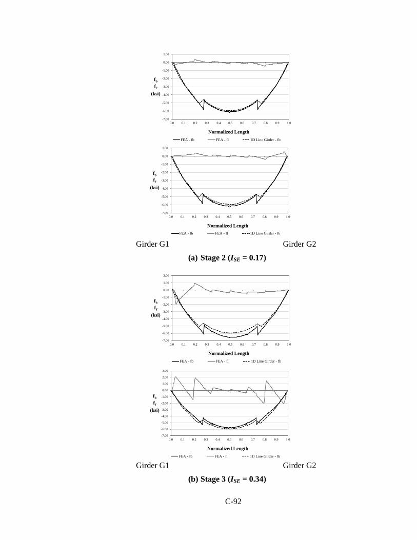
C-92

Girder G1 Girder G2

(a) Stage 2 (ISE = 0.17)

Girder G1 Girder G2

(b) Stage 3 (ISE = 0.34)

-7.00

-6.00

-5.00

-4.00

-3.00

-2.00

-1.00

0.00

1.00

0.0 0.1 0.2 0.3 0.4 0.5 0.6 0.7 0.8 0.9 1.0

fb

f

(ksi)

Normalized LengthFEA - fb FEA - fl 1D Line Girder - fb

-7.00

-6.00

-5.00

-4.00

-3.00

-2.00

-1.00

0.00

1.00

0.0 0.1 0.2 0.3 0.4 0.5 0.6 0.7 0.8 0.9 1.0

fb

f

(ksi)


-7.00

-6.00

-5.00

-4.00

-3.00

-2.00

-1.00

0.00

1.00

2.00

0.0 0.1 0.2 0.3 0.4 0.5 0.6 0.7 0.8 0.9 1.0

fb

f

(ksi)


-7.00

-6.00

-5.00

-4.00

-3.00

-2.00

-1.00

0.00

1.00

2.00

3.00

0.0 0.1 0.2 0.3 0.4 0.5 0.6 0.7 0.8 0.9 1.0

fb

f

(ksi)


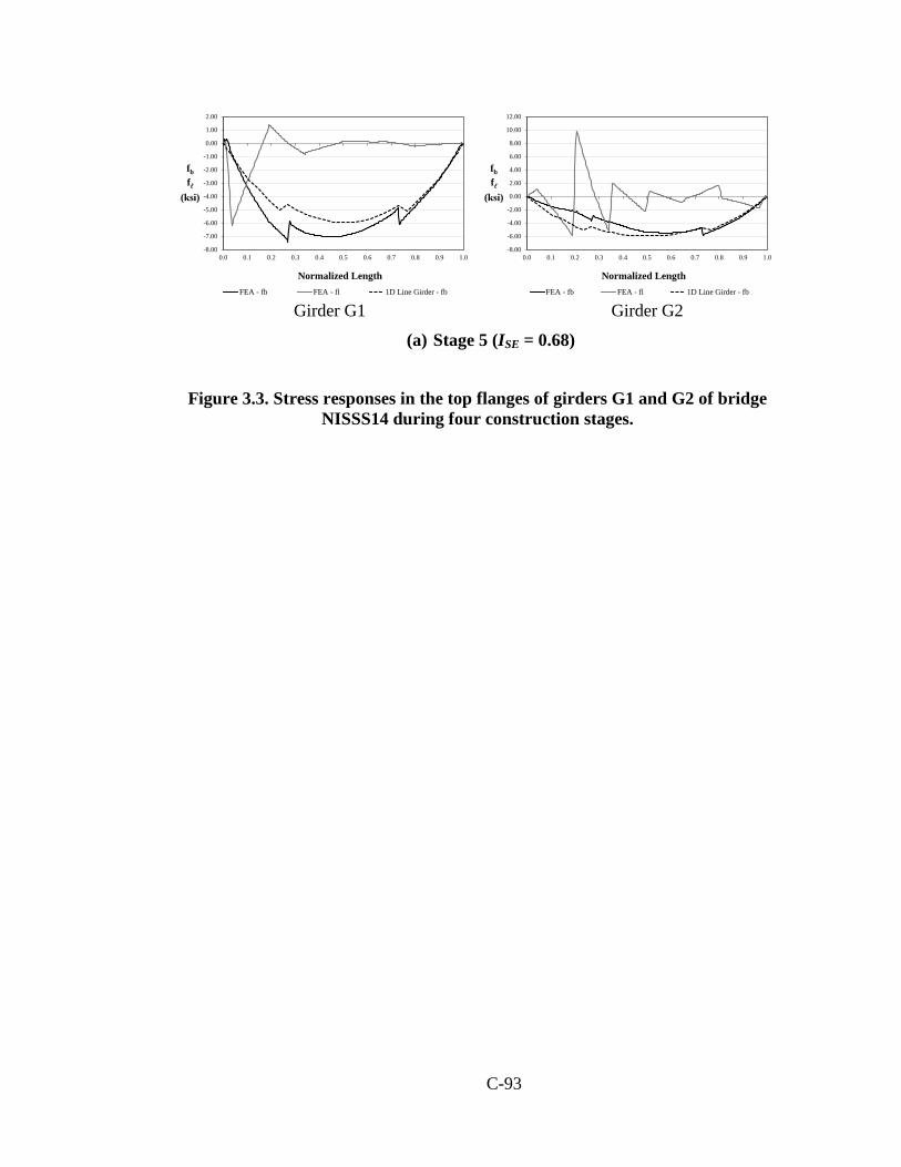
C-93

Girder G1 Girder G2

(a) Stage 5 (ISE = 0.68)

Figure 3.3. Stress responses in the top flanges of girders G1 and G2 of bridge NISSS14 during four construction stages.

-8.00

-7.00

-6.00

-5.00

-4.00

-3.00

-2.00

-1.00

0.00

1.00

2.00

0.0 0.1 0.2 0.3 0.4 0.5 0.6 0.7 0.8 0.9 1.0

fb

f

(ksi)


-8.00

-6.00

-4.00

-2.00

0.00

2.00

4.00

6.00

8.00

10.00

12.00

0.0 0.1 0.2 0.3 0.4 0.5 0.6 0.7 0.8 0.9 1.0

fb

f

(ksi)


C-94

Girder G1 Girder G2

(b) Stage 9 (ISE = 1.36)

Figure 3.3 (continued). Stress responses in the top flanges of girders G1 and G2 of bridge NISSS14 during four construction stages.

The above analyses also demonstrate that the behavior of a skewed bridge

depends on more than just the severity of the skew. The skew angle by itself does not

determine the magnitude of the collateral skew effects. Instead, it is the combination of

the span length, the bridge width (between the fascia girders), the skew angle, and the

distribution of the cross-frames in the bridge layout that determines the structural

behavior. The proposed skew index relates the first three of these parameters, which

define the geometry of the bridge. As discussed, as the index increases, so does the

influence of the skew on the system response. Also, it should be noted that in the

construction stages investigated for this bridge, the responses in Stages 5 and 9, which

have indexes of 0.68 and 1.36, are more significantly affected by the skew compared to

Stages 2 and 3, where the index is close to and less than 0.30.

The above construction simulation also highlights an important aspect regarding

the accuracy of the 1D model predictions. By comparing the predictions obtained from

the 1D and 3D analyses, it is observed that even when the line girder solution deviates

from the physical response, in general, the difference in the major-axis bending stress

magnitudes tends to be minor. For example, at the mid-span of girder G1, Stage 9, the fb

stress obtained from the 3D model is -6.65 ksi. At the same position, the 1D model

predicts a stress of -5.96 ksi, resulting in a difference of 0.69 ksi. For design purposes,

this difference is negligible. Therefore, many engineers would conclude that the 1D

-8.00

-7.00

-6.00

-5.00

-4.00

-3.00

-2.00

-1.00

0.00

1.00

2.00

0.0 0.1 0.2 0.3 0.4 0.5 0.6 0.7 0.8 0.9 1.0

fb

f

(ksi)


-10.00

-5.00

0.00

5.00

10.00

15.00

0.0 0.1 0.2 0.3 0.4 0.5 0.6 0.7 0.8 0.9 1.0

fb

f

(ksi)


C-95

model is sufficient to represent the expected structural behavior of this bridge. However,

it is important to notice that the 1D model does not provide any information regarding the

cross-frame forces and girder flange lateral bending stresses, which according to the

AASHTO Specifications must be included in the construction checks when the lateral

bending is significant. Hence, although the 1D analysis may capture approximately the

major-axis bending response of the girders, it does not provide the information needed to

design all the structural components. Additional studies that show the validity of the skew

index as a method used to characterize the influence of skew on the structural behavior

are provided in Sanchez (2011).

3.1.3 Connectivity Index, IC

The studies conducted in the NCHRP 12-79 research show that in curved radially

supported I-girder bridges, the cross-frame spacing (or the number of intermediate cross-

frames within the span) is a key indicator of the accuracy of the results obtained from 2D-

grid analyses. In conventional 2D-grid models, the representation of the torsional

stiffness of the I-girders is dramatically underestimated since the contributions of

warping to the girder stiffness are neglected. If the bridge is significantly curved and/or

the girders are not closely connected by cross-frames, the results obtained from these 2D-

grid models do not properly represent the structural behavior of the curved bridge during

construction. Chapter 6 provides an extensive discussion regarding this topic. The errors

are tied largely to the coupling between major-axis bending and torsion in curved girders.

A trend that is noticeable in curved radially supported bridges is that the accuracy

of the analysis is roughly proportional to the radius of curvature, R, and to the span length

to unbraced length ratio, Ls / Lb. In a straight bridge connected with a typical number of

cross-frames needed to make the structure behave as a unit, R = ∞ and the Ls /Lb ratio is

large. Also, the accuracy of the results obtained from 2D-grid models should be within

acceptable limits. On the other hand, if the structure has a tight radius of curvature and/or

is connected with a small number of cross-frames, giving a smaller Ls /Lb ratio, the results

of the conventional 2D-grid models may be suspect. In addition, continuous-span I-girder

bridges tend to be able to tolerate smaller values of R and Ls /Lb for a given error

tolerance.

C-96

Based on the above observations, the following ad hoc connectivity index is

proposed to characterize when the results from a 2D-grid analysis may not be sufficiently

accurate:

mnRLL

mRI

cfs

avgbC )1(

000,1511000,15 .

+== (3.2)

where R is the radius of curvature of the bridge centerline in units of ft., m is a constant

equal to 1 for simple-span bridges and 2 for continuous-span bridges, Lb.avg is the average

unbraced length between the cross-frames within the span, Ls is the span length at the

bridge centerline, and ncf is the number of intermediate cross-frames within the span. In

continuous-span bridges, R and ncf can vary from span to span. Therefore, IC is calculated

for each span, and the largest value is taken as the index for the full bridge.

In the NCHRP 12-79 studies, 14 curved radially-supported I-girder bridges were

studied to determine the ability of the simplified methods to capture the responses

predicted by refined 3D models (see Chapter 4 of this report, and Appendices E and I of

the NCHRP 12-79 Final Report). From the results of this study it was determined that

bridges with IC > 1 tend to exhibit large errors from conventional 2D-grid analyses, while

for IC < 1, the 2D-grid analysis predictions are significantly better. Chapter 5 discusses

the categorization of the curved and radial bridges as function of IC in further detail.

To illustrate the use of this index, consider Bridge EISCR1 depicted in Figure

3.4a. This is a simple-span bridge with a radius of curvature equal to 200 ft. The girders

are connected with five cross-frames. For this structure, IC = 15,000/200/(3+1) = 18.75;

therefore a conventional 2D-grid analysis may not be sufficient to capture the expected

behavior. Conversely, Figure 3.4b shows the plan view of Bridge EICCR15, a two-span

structure with 10 intermediate cross-frames in the first span and 13 intermediate cross-

frames in the second. For this bridge, IC1 = 15,000/1,921/2/(10+1) = 0.35 and IC2 =

15,000/1,921/2/(13+1) = 0.28. Therefore, IC = 0.35 < 1.0. Hence, the results obtained

from the 2D-grid analyses should closely represent the benchmark responses.

The connectivity index is determined empirically based on the NCHRP 12-79

studies. In essence, this index evaluates “how curved is the bridge?” and “how well

C-97

connected are the girders?” for conventional 2D-grid analysis purposes. It should not be

used for any other purpose than identifying I-girder bridges where the results of a

conventional 2D-grid analysis may or may not be reliable. It is not intended to be used in

design to determine the number of cross-frames or the cross-frame spacing, for example,

since it applies only to assessment of the inadequacies of the traditional 2D-grid

calculations. It is emphasized that if a 3D analysis (or a 2D-grid analysis including the

recommendations of Chapter 6) is conducted, the engineer will have the required

information to dimension the structural members and check the different strength and

serviceability limit states according to the requirements of the AASHTO LRFD

Specifications, regardless of whether IC is above or below 1.0.

L1 = 90 ft. / R = 200 ft. / w = 23.5 ft.

(a) Bridge EISCR1

L1 = 210 ft., L2 = 271 ft. / R = 1921 ft. / w = 48.9 ft.

(b) Bridge EICCR15 Figure 3.4. Examples for the calculation of IC in curved and radial bridges.

3.1.4 Torsion Index, IT

Regarding the characterization of horizontal curvature effects on the bridge

behavior and the corresponding analysis accuracy, the non-dimensional factor Ls/R,

which is the subtended angle of a span’s centerline expressed in radians, is important (see

Figure 3.5). However, the maximum practical values of Ls/R can vary substantially as a

function of the width of the structural system. The maximum Ls/R is more limited in

relatively narrow bridges because of the greater tendency for overall overturning of the

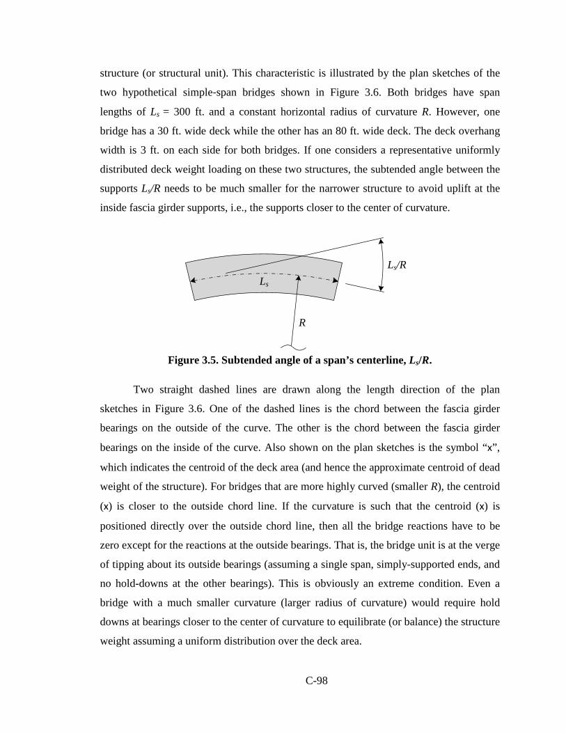
C-98

structure (or structural unit). This characteristic is illustrated by the plan sketches of the

two hypothetical simple-span bridges shown in Figure 3.6. Both bridges have span

lengths of Ls = 300 ft. and a constant horizontal radius of curvature R. However, one

bridge has a 30 ft. wide deck while the other has an 80 ft. wide deck. The deck overhang

width is 3 ft. on each side for both bridges. If one considers a representative uniformly

distributed deck weight loading on these two structures, the subtended angle between the

supports Ls/R needs to be much smaller for the narrower structure to avoid uplift at the

inside fascia girder supports, i.e., the supports closer to the center of curvature.

Figure 3.5. Subtended angle of a span’s centerline, Ls/R.

Two straight dashed lines are drawn along the length direction of the plan

sketches in Figure 3.6. One of the dashed lines is the chord between the fascia girder

bearings on the outside of the curve. The other is the chord between the fascia girder

bearings on the inside of the curve. Also shown on the plan sketches is the symbol “x”,

which indicates the centroid of the deck area (and hence the approximate centroid of dead

weight of the structure). For bridges that are more highly curved (smaller R), the centroid

(x) is closer to the outside chord line. If the curvature is such that the centroid (x) is

positioned directly over the outside chord line, then all the bridge reactions have to be

zero except for the reactions at the outside bearings. That is, the bridge unit is at the verge

of tipping about its outside bearings (assuming a single span, simply-supported ends, and

no hold-downs at the other bearings). This is obviously an extreme condition. Even a

bridge with a much smaller curvature (larger radius of curvature) would require hold

downs at bearings closer to the center of curvature to equilibrate (or balance) the structure

weight assuming a uniform distribution over the deck area.

Ls

R

Ls/R

C-99

The following “torsion index” is an indicator of the overall magnitude of the

torsion within a bridge (or bridge unit) span, and is a strong indicator of the tendency for

uplift at the bearings:

coci

ciT ss

sI

+= (3.3)

Figure 3.6. Plan geometries of two representative simple-span horizontally-curved

bridges with Ls = 300 ft.

The terms in this equation, illustrated in Figure 3.7, are:

• sci, the distance between the centroid of the deck and the chord between the

inside fascia girder bearing locations, measured at the bridge mid-span

perpendicular to a chord between the intersections of the deck centerline with the

bearing lines, and

• sco, the distance between the centroid of the deck and the chord between the

outside fascia girder bearing locations, measured at the bridge mid-span perpen-

dicular to a chord between the intersections of the deck centerline with the

bearing lines.

Ls = 300 ft, w = 30 ft, wg = 24 ft, R = 1000 ft, Ls/R = 0.30

Ls = 300 ft, w = 80 ft, wg = 74 ft, R = 353 ft, Ls/R = 0.85

Fascia Girder (Typ.)Deck Centroid

Deck Centerline

C-100

Figure 3.7. Illustration of terms in the equation for IT.

A value of IT = 0.5 means that the centroid of the deck area is mid-way between the

chords intersecting the outside and inside end bearings. This is the ideal case where the

radius of curvature is equal to infinity and the skew is zero, i.e., a straight tangent bridge.

A value of IT = 1.0 means that the centroid of the deck area is located at the chord line

between the outside bearings. This implies that the bridge is at incipient overturning

instability, by rocking about its outside bearings under uniform self-weight. For a curved

radially-supported span, the denominator in Eq. (3.3), sci + sco, is equal to wg cos(Ls/2R).

As noted above, the torsion index is related to the magnitude of the overall torsion

that exists in the bridge (or bridge unit) span, due to the eccentricity of its self-weight.

Furthermore, it is a strong indicator of the potential for uplift at the inside bearings. In the

NCHRP 12-79 research, it has been observed that simple-span I-girder bridges with a

torsion index of 0.65 and higher are susceptible to uplift at the bearings (Ozgur, 2011).

Continuous-span bridges can tolerate higher indices due to the stabilizing effect of the

continuity with the adjacent spans. However, the continuity with the adjacent spans

generally varies during the steel erection. The torsion index can be calculated for an

intermediate steel erection stage using the width between the outside and inside girders

during that stage. IT > 0.65 can serve as a rough indicator of when the engineer should

check carefully for uplift during the stage.

Tub-girder bridge bearings are typically closer to the bridge centerline and also

tub girders are more efficient at resisting overall torsion; therefore, the torsion index in

tub-girder bridges tends to be larger than that for an I-girder bridge with the same deck

geometry.

Fascia Girder (Typ.)Deck Centroid

Deck Centerline

sci

sco

C-101

3.1.5 Girder Length Index, IL

The last key index recommended in the NCHRP 12-79 research for characterizing

the demands on the methods of analysis with respect to the handling of curvature and

skew effects is the girder length index, IL. This index is usually expressed as

S

LL L

LI = (3.4)

where LL is the span length of the longest fascia girder and LS is the span length of the

shortest fascia girder within each span. For the curved and skewed bridges considered in

the NCHRP 12-79 project research, this definition is modified to

ng

L LLI 1= (3.5)

where L1 is the span length of fascia girder number 1, and Lng is the span length of the

highest numbered fascia girder. In the NCHRP 12-79 research, all the curved bridges are

displayed in a “concave up” orientation with girder G1 located on the outside of the curve

at the bottom of the sketch. Therefore, for the curved radially-supported bridges, IL is

generally somewhat larger than 1.0. If a bridge is curved and skewed, IL is increased from

this value if the skew increases the length of the outside fascia girder. Correspondingly, IL

is decreased and may be less than 1.0 if the fascia girder on the outside of the curve is

decreased in length by the skew.

In continuous-span bridges, one index is determined for each span, and the value

most different from 1.0 is used to represent the bridge.

The NCHRP 12-79 studies actually indicate that the previous four indices are

sufficient to form decisions about the selection of the different methods of analysis.

However, the girder length index IL is an additional parameter indicative of the tendency

for differential vertical deflections across the bridge width. The value of IL is 1.0 for

straight bridges with parallel bearing lines, whereas it can be a relatively large number if

the bridge is wide and has a significant difference between the skew of adjacent bearing

lines. Therefore, one might expect that of two bridges with a large skew index, IS, the

C-102

demands on the analysis may be greater if the index IL is larger. This trend is not borne

out in the NCHRP project studies however. It is believed that the satisfaction of the

AASHTO Specification requirements in the bridge designs diminishes the importance of

IL.

3.2 Other Factors

The second and third indices discussed in Section 3.1 (IS and IC) are the basis of

the scoring system presented in Chapter 5 to assess the ability of the approximate

methods to capture the structural responses during the construction of steel I-girder

bridges. The first index, AFG, is used as an indicator of when second-order amplification

of the responses may be significant, and the fourth index, (IT) is used as an indicator of

when bearing uplift considerations may be particularly significant. In addition to these

indices, NCHRP 12-79 investigated the influence of various other factors that may affect

the structural behavior and the analysis accuracy during construction. Span length, radius

of curvature, support skew, number of spans and other parameters were variables

considered to assess the geometry of the bridges included in the research studies. Chapter

4 discusses these parameters in detail along with criteria for the selection of the bridge

geometries that were studied.

C-104

4. Design of NCHRP 12-79 Analytical Studies

4.1 Introduction

Curved and/or skewed bridge structures with different geometries can respond in

dramatically different ways during their various stages of construction; therefore,

extensive studies of a wide range of bridge structures are necessary to gain a true

understanding of the accuracy of different analysis methods and the effect of this

accuracy on the structural performance.

It should be emphasized that both over-prediction and underprediction of

displacements can be equally bad in cases where certain relative deflections are critical.

Furthermore, one should not specify a simple blanket accuracy requirement on all the

analysis deflections. Specific deflections should be considered, and in cases where the

deflections are sufficiently small, larger inaccuracies can be tolerated.

It is important that the accuracy of simplified analysis methods be evaluated using

actual bridge designs that satisfy either prior and/or current AASHTO design criteria. The

results of simply varying bridge parameters without checking Specification requirements

can be misleading. AASHTO requirements must be satisfied for the study bridges to

allow the research to establish appropriate relationships between bridge design variables

and recommended levels of analysis and construction engineering effort.

One of the early tasks of NCHRP 12-79 was to identify existing bridges

representing a spectrum of various combinations of span arrangement, span length,

curvature, bridge widths and skew. It was desired to consider both simple and

continuous-spans, and that preference would be given to bridges that had:

• Good instrumented field data or at least good field observations, particularly data

and observations during intermediate stages of construction and

• Detailed construction plans,

and in which

C-105

• The design and construction satisfied prior and/or current AASHTO

Specifications and established recommendations, yet construction challenges were

encountered or certain attributes resulted in concerns about the final state of stress

in the girders, etc.

Bridges where technical challenges were addressed very successfully as well as

cases where there were some significant problems were sought. However bridges

involving generally acknowledged poor practices, e.g., inappropriate use of oversize or

slotted holes, inadequate attachment of cross-frames during construction, etc., were not

considered. The focus of Project 12-79 was on analysis and design using appropriate

practices. Analysis requirements for forensic investigation of bridges with faulty details

were not addressed. However, it was desired for the studies to shed light on the ability of

analysis methods to highlight faulty erection schemes, etc., given appropriate design

details.

Once the above existing bridge collection effort was completed, then the geometric

factors influencing the analysis, design and construction of the bridges were identified.

Finally, the ranges and number of levels of these factors were selected for subsequent

analytical study.

The following sections provide a detailed description of each of the above steps.

4.2 Identification and Collection of Existing Bridges

Figures 4.1 through 4.6 summarize the overall characteristics of the existing I-

girder bridges contributed to NCHRP 12-79 from various owners and consultants. These

figures show sketches of the overall plan geometry of the deck and of the bearing lines.

Although the number of pages used to illustrate the various geometries is relatively large,

these sketches convey a great deal of useful information in a succinct fashion. All the

linear dimensions indicated in the sketches are provided in units of feet and all the

angular dimensions are provided in degrees. These figures subdivide the collected

existing I-girder bridges into the following categories:

C-106

• Simple-span, Straight, with Skewed supports (ISSS),

• Continuous-span, Straight, with Skewed supports (ICSS),

• Simple-span, Curved, with Radial supports (ISCR),

• Continuous-span, Curved, with Radial supports (ICCR),

• Simple-span, Curved, with Skewed supports (ISCS), and

• Continuous-span, Curved, with Skewed supports (ICCS).

Each of the bridge sketches in Figures 4.1 through 4.6 has a title block containing

the following information:

1. An identification label, composed of the letter “E” for “Existing” followed by the

above symbols indicating the bridge category, and ending with the bridge number

for that category, e.g., bridge “EISCR1” in Figure 4.3.

2. A description of the structure, composed of the bridge name and/or location.

3. A summary of the basic geometry information about the bridge, enclosed in

parentheses. For instance, in Figure 4.3, the basic geometry information for the

single EISCR bridge includes:

• The span length of the bridge centerline (measured along the horizontal

curve),

• The horizontal radius of curvature of the bridge centerline, and

• The out-to-out width of the bridge deck perpendicular to the bridge

centerline.

This information is conveyed symbolically in the figure caption as

“(LENGTH/RADIUS/WIDTH).” The other categories have similar but different

basic geometry information. This information is summarized symbolically in each

of their figure captions. The skew angle of the bearing lines is represented by the

symbol θ. This angle is taken as zero when a bearing line is perpendicular to the

centerline of the structure, that is, when the bearing line does not have any skew.

4. The symbol “*”, at the end of the parentheses delimiting the basic geometry

information, if the bridge has erection plans. No symbol is shown if the bridge

does not have erection plans.

C-107

5. The organization that provided the drawings for each bridge. This information is

delimited by square brackets, i.e., “[FHWA]” in Figure 4.3.

Other pertinent information is provided underneath the plan sketch of each of the

bridges. This information includes data such as the number of girders in the bridge cross-

section, whether test or field data is available for the structure, references to papers or

reports containing test data or documentation of previous research on the bridge, and

brief notes regarding successes or difficulties for certain bridges. Note that one scale is

utilized for all the simple-span bridges, whereas a slightly smaller scale is used for all the

continuous-span bridges.

Figures 4.7 through 4.12 summarize the overall characteristics of the existing tub-

girder bridges. These figures are organized in a similar fashion to Figures 4.1 through 4.6.

The various existing bridges shown in Figures 4.1 through 4.12 served two

purposes:

1. The composite of all the existing bridges was an aid to the project team in

gauging the range and level of geometries that should be considered within the

main parametric studies of the Project.

2. A number of the existing bridges that best fit the Project’s criteria for the

analytical studies, discussed in Section 4.1, were selected for detailed study and

inserted into the complete parametric study matrix, discussed subsequently in this

chapter.

One can observe that there is a significant diversity of geometries among the

existing bridges. This is particularly true for the skewed bridges. It was clear from these

sketches that both the skew angle and the skew pattern (i.e., radial, non-radial, parallel

and non-parallel bearing arrangements) must be studied. It was not sufficient to focus

solely on bridges with parallel bearing lines if the complete implications of skew were to

be addressed.

C-108

(EISSS 5) SR 0581 Section A01, Cumberland Co., PA (123/43.8/-59.7,-59.7), (123/43.8/-59.7,-59.7) [PennDOT]

10 girders, Phased Construction, Difficulty with concrete cover during deck

replacement

(EISSS 4) Bridge No. Sum-8-1724 B, Ramp B over Brandywine Creek, Summit Co., OH(120 / 51 / -60, -60) [ODOT]

6 girders, Semi-integral abutments

(EISSS 1) I-30 (WB & EB) over Baseline road I-430 - Geyer Springs Rd., Pulaski Co., AR(242 / 59.1 / 64.0, 64.0) [AHTD]

(EISSS 3) Bridge on SR 1003 (Chicken Road) over US74 between SR 1155 & SR 1161, Robeson Co., NC(133 / 30.1 / -46.2, -46.2) [NCDOT]

4 girders, has similar adjacent simple span,Field data available (Sumner NCSU), Undesirable

girder layover & bowing of girder webs

(EISSS 2) Bridge over I-85 & US70 on West Bound Ramp between SR 1400 & N-S Railway-Span 4, Durham Co., NC (135 / 41.1 / -65.3, -65.3) [NCDOT]

5 girders, has similar adjacent simple spans

Scale in feet

0 20 50 100

(EISSS 6) I-87 / I-287, Westchester Co., NY (254 / 50.8 / -65.0, -60.5) * [NYDOT]

8 girders, Succesful implementation of TDLF detailing

* Bridge has detailed erection plans.

Figure 4.1. Existing I-girder bridges, Simple-span, Straight with Skewed supports,

(EISSS #) Description (LENGTH / WIDTH / θLeft, θRight) [Source].

(267 / 58 / 62.3, 62.3)* [NYDOT]

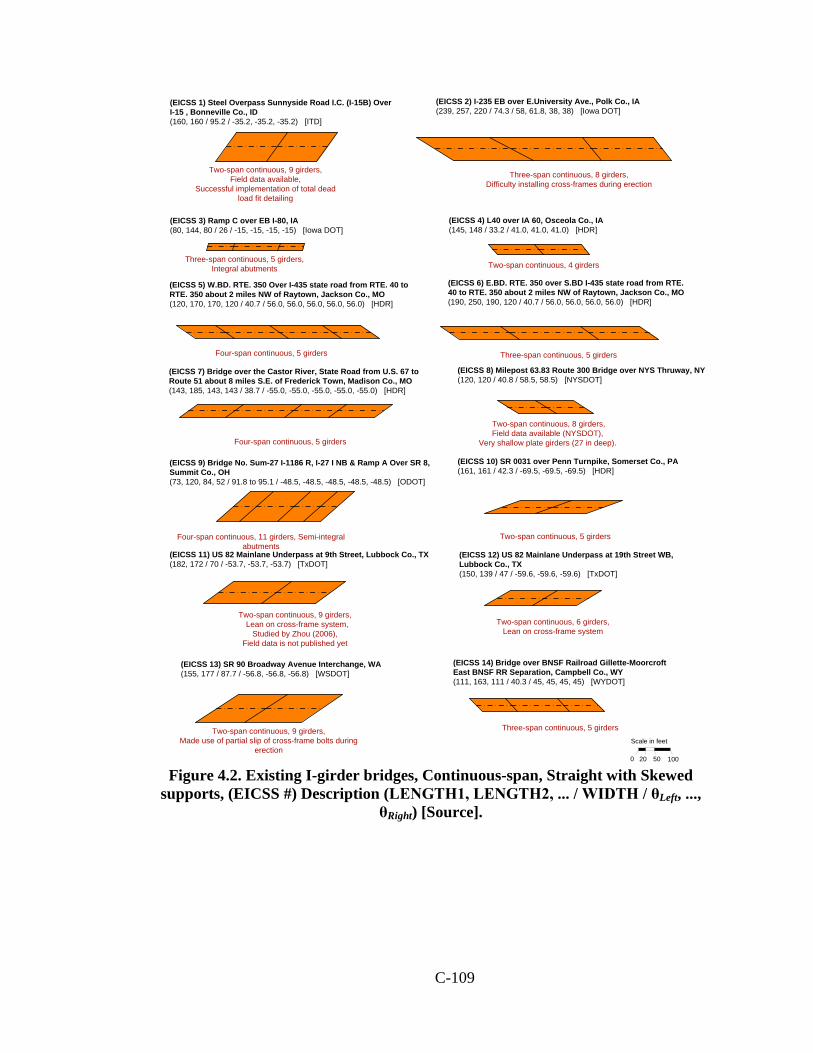
C-109

(EICSS 10) SR 0031 over Penn Turnpike, Somerset Co., PA(161, 161 / 42.3 / -69.5, -69.5, -69.5) [HDR]

Two-span continuous, 5 girders

(EICSS 11) US 82 Mainlane Underpass at 9th Street, Lubbock Co., TX(182, 172 / 70 / -53.7, -53.7, -53.7) [TxDOT]

Two-span continuous, 9 girders, Lean on cross-frame system,

Studied by Zhou (2006), Field data is not published yet

(EICSS 12) US 82 Mainlane Underpass at 19th Street WB, Lubbock Co., TX (150, 139 / 47 / -59.6, -59.6, -59.6) [TxDOT]

Two-span continuous, 6 girders, Lean on cross-frame system

(EICSS 2) I-235 EB over E.University Ave., Polk Co., IA (239, 257, 220 / 74.3 / 58, 61.8, 38, 38) [Iowa DOT]

Three-span continuous, 8 girders,Difficulty installing cross-frames during erection

(EICSS 14) Bridge over BNSF Railroad Gillette-Moorcroft East BNSF RR Separation, Campbell Co., WY(111, 163, 111 / 40.3 / 45, 45, 45, 45) [WYDOT]

Three-span continuous, 5 girders

(EICSS 3) Ramp C over EB I-80, IA (80, 144, 80 / 26 / -15, -15, -15, -15) [Iowa DOT]

Three-span continuous, 5 girders, Integral abutments

(EICSS 13) SR 90 Broadway Avenue Interchange, WA(155, 177 / 87.7 / -56.8, -56.8, -56.8) [WSDOT]

Two-span continuous, 9 girders,Made use of partial slip of cross-frame bolts during

erection

(EICSS 9) Bridge No. Sum-27 I-1186 R, I-27 I NB & Ramp A Over SR 8, Summit Co., OH(73, 120, 84, 52 / 91.8 to 95.1 / -48.5, -48.5, -48.5, -48.5, -48.5) [ODOT]

Four-span continuous, 11 girders, Semi-integral abutments

(EICSS 1) Steel Overpass Sunnyside Road I.C. (I-15B) Over I-15 , Bonneville Co., ID (160, 160 / 95.2 / -35.2, -35.2, -35.2) [ITD]

Two-span continuous, 9 girders, Field data available,

Successful implementation of total dead load fit detailing

(EICSS 5) W.BD. RTE. 350 Over I-435 state road from RTE. 40 to RTE. 350 about 2 miles NW of Raytown, Jackson Co., MO (120, 170, 170, 120 / 40.7 / 56.0, 56.0, 56.0, 56.0, 56.0) [HDR]

Four-span continuous, 5 girders

(EICSS 6) E.BD. RTE. 350 over S.BD I-435 state road from RTE. 40 to RTE. 350 about 2 miles NW of Raytown, Jackson Co., MO(190, 250, 190, 120 / 40.7 / 56.0, 56.0, 56.0, 56.0) [HDR]


(EICSS 7) Bridge over the Castor River, State Road from U.S. 67 to Route 51 about 8 miles S.E. of Frederick Town, Madison Co., MO (143, 185, 143, 143 / 38.7 / -55.0, -55.0, -55.0, -55.0, -55.0) [HDR]


(EICSS 4) L40 over IA 60, Osceola Co., IA(145, 148 / 33.2 / 41.0, 41.0, 41.0) [HDR]


(EICSS 8) Milepost 63.83 Route 300 Bridge over NYS Thruway, NY (120, 120 / 40.8 / 58.5, 58.5) [NYSDOT]

Two-span continuous, 8 girders, Field data available (NYSDOT),

Very shallow plate girders (27 in deep).

Scale in feet

0 20 50 100 Figure 4.2. Existing I-girder bridges, Continuous-span, Straight with Skewed

supports, (EICSS #) Description (LENGTH1, LENGTH2, ... / WIDTH / θLeft, ..., θRight) [Source].

C-110

(EISCR 1) FHWA Test Bridge (90 / 200 / 23.5) * [FHWA]

3 girders, Test data available (Jung 2006), Bridge designed to a number if limits of the AASHTO LRFD

Specifications

0 20 50 100

Scale in feet

Figure 4.3. Existing I-girder bridges, Simple-span, Curved with Radial supports,

(EISCR #) Description (LENGTH / RADIUS / WIDTH) [Source].

(EICCR 2) Ramp S-W I-10 to Encanto - Unit 2, AZ (146, 213, 213, 151 / 768 / 31.2) [HDR]


(EICCR 3) Ramp W-N I10 to Encanto, AZ (170, 199, 209, 170 / 762 / 39.2) [HDR]


(EICCR 5) I-80 / I-480 / Kennedy Freeway Interchange - Unit 8A, Douglas Co. NE (126, 176, 176, 176, 126 / 769 / 36.5) [HDR]

Five-span continuous, 3 girders

(EICCR 1) Ramp E-N I-10 to Encanto - Unit 2, AZ(147, 163, 142, 138 / 877 / 31.2) [HDR]


(EICCR 6) I-80 / I-480 / Kennedy Freeway Interchange - Unit 7B, Douglas Co., NE (190, 241, 189 / 813 / 36.5) [HDR]


(EICCR 8) Bridge No. Sum-8-1758 A, Ramp A over Highland Road, Indian Creek & Ramp R3, Summit Co., OH(125, 180, 180, 180, 125 / 1347 / 49)* [ODOT]


(EICCR 4) Ramp GG John F. Kennedy Memorial Highway, I-95 Express Toll Lanes and I-695 Interchange, Baltimore Co., MD(222, 260, 210, 162, 256, 190 / 1108, ∞ / 44)* [HSSI]

Six-span continuous, 5 girders, Field observations available (Cisneros, White & Ozgur)

(EICCR 7) Suffern Interchange Ramp C, I-287 / Thruway / Route 17 Interchange - Unit 2, Rockland Co., NY(123, 167, 123 / 700 / 41.6) [NYSDOT]

Three-span continuous, 5 girders,Uplift issues encountered during erection

* Bridge has detailed erection plans.Scale in feet

0 20 50 100 Figure 4.4. Existing I-girder bridges, Continuous-span, Curved with Radial supports, (EICCR #) Description (LENGTH1, LENGTH2, ... / RADIUS1,

RADIUS2, .../ WIDTH) [Source].

C-111

(EICCR 11) Ford City Bridge, Ford City, PA (321, 445, 292 / ∞, 511/ 48.2) * [HDR]

Three-span continuous, 4 girders, Flange lateral bracing system, Studied by Chavel and Earls (2006 a & b & 2001),

Field observations available

(EICCR 13) Mon / Fayette Expressway Uniontown to Brownsville SR 0043 Section 51A1 Ramp S-119N over Ramp 51-119N, SR 0119, Ramp 119S-51 and SR 0051- Unit 15, Fayette Co., PA (108, 137, 150, 104 / 756 / 42.4) [HDR]

(EICCR 14) Mon / Fayette Expressway Uniontown to Brownsville SR 0043 Section 51A1 Ramp S-119N over Ramp 51-119N, SR 0119, Ramp 119S-51 and SR 0051- Unit 16, Fayette Co., PA (141, 235, 176, 101 / 756 / 42.4) [HDR]

Four-span continuous, 5 girders, Not yet built Four-span continuous, 5 girders, Not yet built

(EICCR 9) Mon / Fayette Expressway Uniontown to Brownsville SR 0043 Section 51A1 Ramp S-119N over Ramp 51-119N, SR 0119, Ramp 119S-51 and Ramp S-119N, Fayette Co., PA (129, 200, 200, 164, 155, 184, 179, 179, 169, 119 / 1366 / 42.4) [HDR]

Ten-span continuous, 5 girders, Not yet built

(EICCR 15) SR 6220 A11 over SR 6220 NB & SB, Centre Co.,PA (210, 271 / 1921 / 48.9)* [HDR]

Two-span continuous, Unbalanced spans, 5 girdersField data available (Shura 2004, Domalik et al. 2005)

(EICCR 12) Bridge over ORT Valley RD, Ramp H SR 0022 EB / WB, SR 0322 EB / WB & Ramp A-2, Mifflin Co., PA(142, 184, 184, 157, 186 / 596 / 37.9)* [HSSI]


(EICCR 10) SR 6060 Section 014 Ramp WS-C Over WS-A. WS-D and SR 6060 - Unit 1, Allegheny Co., PA (226, 226, 149 / 813 / 34.5) [HDR]



Scale in feet

0 20 50 100 Figure 4.4. (continued). Existing I-girder bridges, Continuous-span, Curved with Radial supports, (EICCR #) Description (LENGTH1, LENGTH2, ... / RADIUS1,


C-112

(EICCR 22) Ramp B over Briley Parkway and Ramp A, Davidson Co., TN (141, 188, 188, 208, 157 / 449 / 44) [TDOT]

Five-span continuous, 5 girders, Significantly curved

(EICCR 21) SR 386 over Shute Lane, SR 6 and CSX Railroad, Sumner Co., TN(237, 296, 237 / 1741 / 43.7) [TDOT]


(EICCR 18) Ramp G Over SR 0022, SR 0079, Campbells Run Road & Ramp F - Unit 1, Allegheny Co., PA (182, 286, 236, 181 / 830 / 32.4)* [PennDOT]

(EICCR 19) Ramp G Over SR 0022, SR 0079, Campbells Run Road & Ramp F - Unit 2, Allegheny Co., PA (206, 225, 208 / 830 / 32.4)* [PennDOT]

Four-span continuous, 5 girders,Study in progress (Linzell)

Three-span continuous, 5 girders,Study in progress (Linzell)

(EICCR 16) SR 6026 Section CO2 over SR 0322 WB, Ramp N-W, SR 3007 & Ramp W-S- Unit 1, Centre Co., PA (238, 334, 298 / 1940 / 46.9) [PennDOT]

(EICCR 17) SR 6026 Section CO2 over SR 0322 WB, Ramp N-W, SR 3007 & Ramp W-S - Unit 2, Centre Co., PA(298, 333, 266 / 1940 / 46.9) [PennDOT]

Three-span continuous, 5 girders, Flange lateral bracing system, Study in progress (Linzell)

Three-span continuous, 5 girders, Flange lateral bracing system, Study in Progress (Linzell)

(EICCR 20) PennDOT Structure #22737 (Structure #7A in construction documentation) at I-99 interchange, State College, PA(296, 333, 266 / 1940 / 45.8)* [Linzell]

Three-span continuous, 5 girders,Flange lateral bracing System, Field data available (Bell 2002)


Scale in feet

0 20 50 100 Figure 4.4. (continued). Existing I-girder bridges, Continuous-span, Curved with Radial supports, (EICCR #) Description (LENGTH1, LENGTH2, ... / RADIUS1,


C-113

(EICCR 26) US Route 340 over Shenandoah River, Harpers Ferry, WV (137, 177, 196, 196, 196, 196, 177, 137 / 1145, -1145 / 52.8 to 55.4) [HSSI]

Eight-span continuous, 5 girders

(EICCR 25) US 35 Flyover Ramp 5, Putnam Co., WV (175, 241, 179, 250, 178, 142 / 941 / 30.5)* [HDR]

Six-span continuous, 4 girders

(EICCR 27) "A" Street Viaduct / Elk Street, Sweetwater Co., WY (119, 164, 164, 119 / 597, ∞ / 71) [WYDOT]

Four-span continuous, 8 girders, Fit-up problems encountered in field

(EICCR 23) LP1604 SE Connector - Unit 2 , Bexar Co., TX(172, 215 / 855 / 30) [HDR]

Two-span continuous, 4 girders, will not be buillt

(EICCR 24) LP1604 NW Connector- Unit2, Bexar Co., TX (160, 195 / 873 / 40) [HDR]

Two-span continuous, 5 girders, will not be buillt


Scale in feet

0 20 50 100

(EICCR 22 a) Bridge No.12 Ramp B over I-40, Robertson Avenue Project, Davidson Co., TN (172, 217, 217, 195, 171, 172, 162, 192 / 791,889,746,766 / 43) * [TDOT]

Eight-span continuous, 5 girders,Field data available (Leon et al. 2011), Field observations available

Figure 4.4. (continued). Existing I-girder bridges, Continuous-span, Curved with Radial supports, (EICCR #) Description (LENGTH1, LENGTH2, ... / RADIUS1,


Field data available (Dykas, 2012), Field observations available

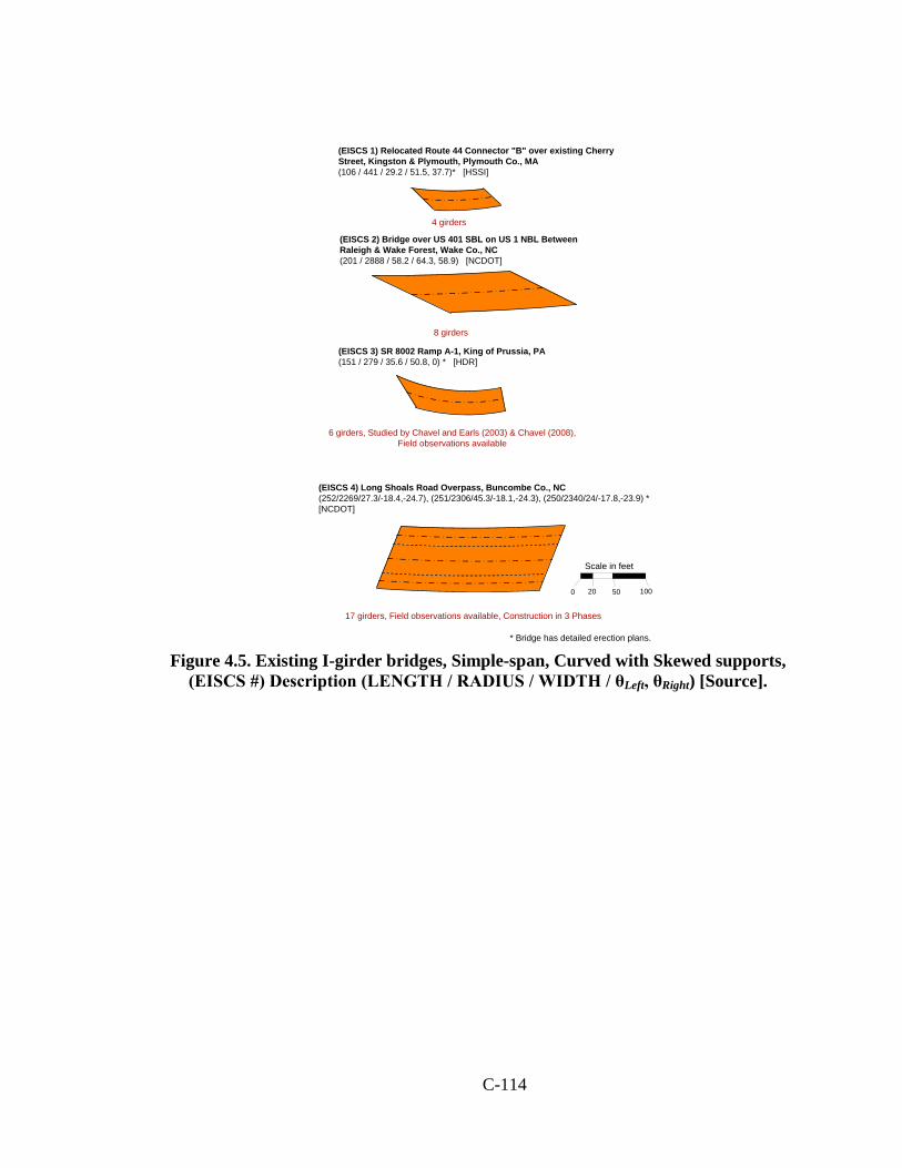
C-114

(EISCS 3) SR 8002 Ramp A-1, King of Prussia, PA (151 / 279 / 35.6 / 50.8, 0) * [HDR]

6 girders, Studied by Chavel and Earls (2003) & Chavel (2008), Field observations available

(EISCS 2) Bridge over US 401 SBL on US 1 NBL Between Raleigh & Wake Forest, Wake Co., NC (201 / 2888 / 58.2 / 64.3, 58.9) [NCDOT]

8 girders

(EISCS 1) Relocated Route 44 Connector "B" over existing Cherry Street, Kingston & Plymouth, Plymouth Co., MA(106 / 441 / 29.2 / 51.5, 37.7)* [HSSI]

4 girders


Scale in feet

0 20 50 100

(EISCS 4) Long Shoals Road Overpass, Buncombe Co., NC (252/2269/27.3/-18.4,-24.7), (251/2306/45.3/-18.1,-24.3), (250/2340/24/-17.8,-23.9) * [NCDOT]

17 girders, Field observations available, Construction in 3 Phases

Figure 4.5. Existing I-girder bridges, Simple-span, Curved with Skewed supports,

(EISCS #) Description (LENGTH / RADIUS / WIDTH / θLeft, θRight) [Source].

C-115

(EICCS 10) Mn / DOT bridge No 27998, TH94 between 27th Avenue and Huron Boulevard, Minneapolis, MN(145, 150 / 286 / 33.4 / 40.1, 34.8, -10.4)* [Galambos & Leon]

Two-span continuous, 4 girders, Field data available (Galambos et al. 1996),

Used by Nowak et al.(2006) in calibration of LRFD Design Specifications for curved steel bridges

(EICCS 1) I-459 / US31 Interchange Flyover A, Jefferson Co., AL(204, 278, 252, 185 / 757 / 40.2 / 0, 0, 32.7, 0, 0)* [ALDOT]

Four-span continuous, 5 girders,Field Observations available (Osborne 2002),

Successful implementation of total dead load fit detailing

(EICCS 2) Northbound Roadway bridge over CSXT railroad on US 331 between Legrand and Montgomery, Montgomery Co., AL (108, 134, 108 / 14280 / 42.7 / -61.4, -61.4, -61.4, -61.4) [ALDOT]

Three-span continuous, 6 girders, Severe deck cracking encountered, requiring complete deck replacement prior to end of

project

(EICCS 6) Ramp C over WB I-80, IA (90, 152, 90 / 1340 / 26 / 35, 35, 35, 35) [Iowa DOT]

(EICCS 8) Ramp B over EB I-80, IA (85, 149, 85 / 950 / 26 / -15, -15, -15, -15) [Iowa DOT]



(EICCS 3) Ramp S-E I-10 to Encanto - Unit 1, AZ (133, 129 / 820 / 39.2 / -25.9, 0, 0) [HDR]


(EICCS 5) WB E-W Connector over I-88, IL (181, 228, 198, 139, 138 / 1134 / 47.2 / -48.8, -60.2, 0, 0, 0, 0) [HDR]

Five-span continuous, 5 girders, Bearing lines nearly 90° in 4th span

(EICCS 9) Ramp D over EB I-80, IA (90, 150, 90 / 1340 / 26 / 35, 35, 35, 35) [Iowa DOT]

(EICCS 7) Ramp A over WB I-80, IA (80, 142, 80 / 950 / 26 / -15, -15, -15, -15) [Iowa DOT]



(EICCS 4) Ramp S-E I-10 to Encanto - Unit 2, AZ(162, 192, 198, 160 / 820 / 39.2 / 0, 0, 0, 0, -25.9) [HDR]


(EICCS 11) Ramp 13 over Route 364, State road from Route 94 to Missouri river in St. Peters, St. Charles Co., MO (104, 138 / 317 / 32.2 / 0, -31.5, -29.5) [HDR]

Two-span continuous, 4 girders * Bridge has detailed erection plans.

Scale in feet

0 20 50 100 Figure 4.6. Existing I-girder bridges, Continuous-span, Curved with Skewed

supports, (EICCS #) Description (LENGTH1, LENGTH2, ... / RADIUS / WIDTH / θLeft, ..., θRight) [Source].

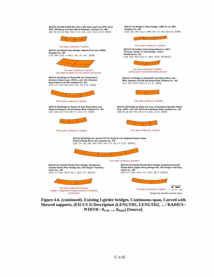
C-116

(EICCS 18) Bridge on Ramp CA over Bryan Blvd, and Ramp D between I-40 and Bryan Blvd, Guilford Co., NC (107, 100, 110 / 754 / 48.4 / 0, -0.5, 0, 0) [HDR]


(EICCS 17) Bridge on Ramp BD over Bryan Blvd. and -RPD- between US 220 and Bryan Blvd, Guilford Co., NC (117, 159 / 1574 / 48.4 / 0, 1.1, 0) [HDR]


(EICCS 21) Grande Ronde River Bridge, Westbound Grande Ronde River Bridge Sec. Old Oregon Trail Hwy., Union Co., OR(253, 177 / 951 / 50.9 / -31.1, -19.4, -27) [ODOT]

Two-span continuous,5 girders,Stage 1, independent bridge structure in a phased

construction

(EICCS 19) Bridge on Ramp CA over, Greensboro Western Urban loop, -RPD-, and -CD- BTN I-40 and Bryan Blvd, Guilford Co., NC (100, 94, 82, 86 / 754 / 48.4 / 0, 0, 8.8, 2.6, 0) [HDR]


(EICCS 16) Bridge on Ramp BD over Greensboro Western Urban Loop, -RPCA-, and -CD- Between Bryan Blvd & US 220, Guilford Co., NC (173, 171, 170 / 754 / 48.4 / 5.6, -2.6, 0, 0) [HDR]


(EICCS 20) Bridge No. Sum-8-1757 B, Ramp B over Highland Road, Indian Creek & Ramp R3 & I-271, Summit Co., OH(115, 170, 151, 182, 146 / 1347 / 49 / 0, 0, -20.7, 0, 0, 0)* [ODOT]


(EICCS 12) SNI-A-BAR Rd. Over I-435 state road from RTE. 40 toRTE. 350 about 3.6 miles NW of Raytown, Jackson Co., MO (60, 102, 92, 50 / 881 / 50.2 / -2.4, -6.4, -13.0, -18.9, -22.3) [HDR]


(EICCS 13) Bridge 5, West Dodge. 129th St. to I-680, Douglas Co., NE(118, 128, 145 / 712, ∞, 699 / 32.7 / 0, 18.4, 18.8, 0) [HDR]


(EICCS 14) Abbott Drive Bridge, Abbott Drive over UPRR, Douglas Co., NE(179, 168 / 1125, ∞ / 85.2 / -38, -42, -42) [HDR]

Two-span continuous, 8 girders,Two different depths of cross-frames and girders

(EICCS 22) Grande Ronde River Bridge, Eastbound Grande Ronde River (Upper Perry) Bridge Sec. Old Oregon Trail Hwy., Union Co., OR (240, 177 / 951 / 42.9 / -6.7, -20.4, -28.7) [ODOT]


(EICCS 15) Suffern Interchange Ramp C, I-287 / Thruway / Route 17 Interchange - Unit 1, Rockland Co., NY(148, 158 / 700 / 41.6 / 0, -49.5, -31.8) [NYSDOT]

Two-span continuous, 5 girders, Uplift issues encountered during erection


Scale in feet

0 20 50 100

Figure 4.6. (continued). Existing I-girder bridges, Continuous-span, Curved with Skewed supports, (EICCS #) Description (LENGTH1, LENGTH2, ... / RADIUS /

WIDTH / θLeft, ..., θRight) [Source].

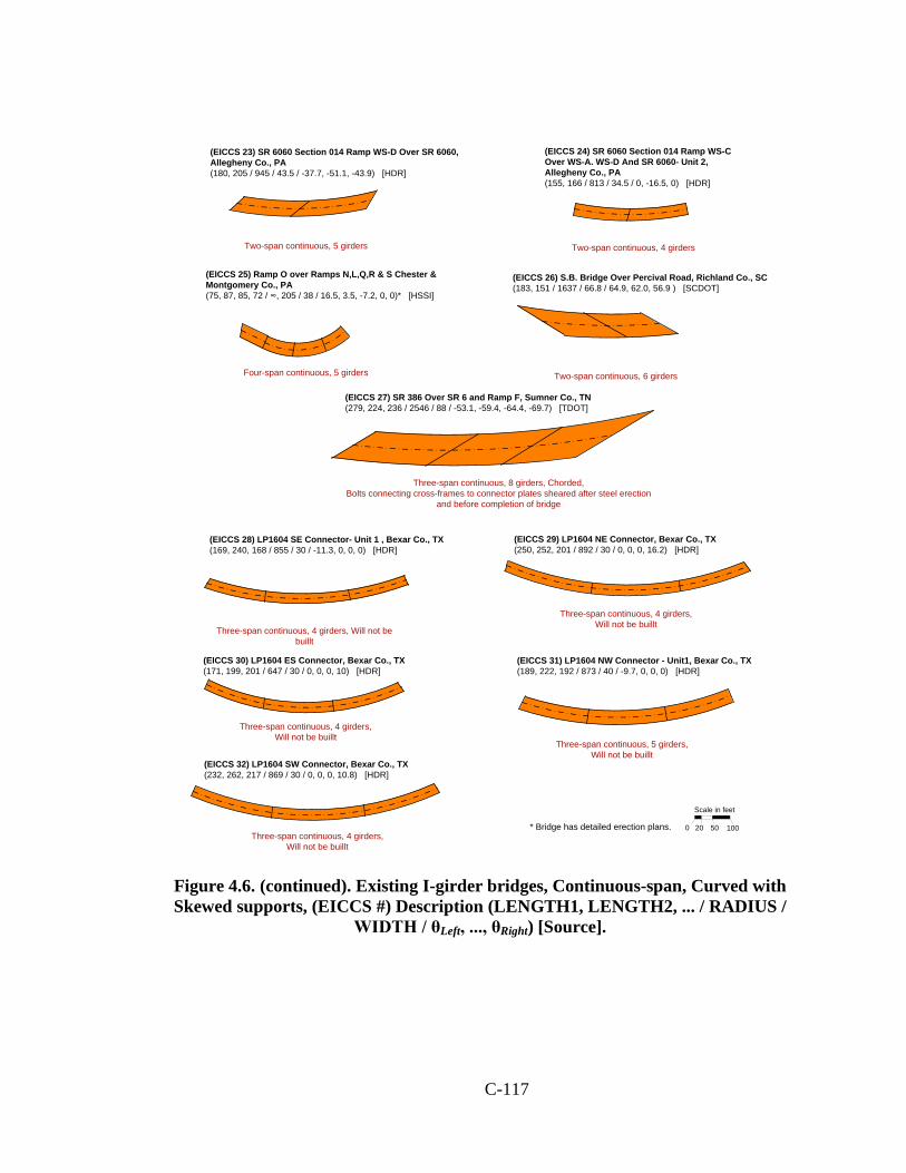
C-117

(EICCS 27) SR 386 Over SR 6 and Ramp F, Sumner Co., TN (279, 224, 236 / 2546 / 88 / -53.1, -59.4, -64.4, -69.7) [TDOT]

Three-span continuous, 8 girders, Chorded,Bolts connecting cross-frames to connector plates sheared after steel erection

and before completion of bridge

(EICCS 28) LP1604 SE Connector- Unit 1 , Bexar Co., TX (169, 240, 168 / 855 / 30 / -11.3, 0, 0, 0) [HDR]

Three-span continuous, 4 girders, Will not be buillt

(EICCS 29) LP1604 NE Connector, Bexar Co., TX (250, 252, 201 / 892 / 30 / 0, 0, 0, 16.2) [HDR]


(EICCS 31) LP1604 NW Connector - Unit1, Bexar Co., TX (189, 222, 192 / 873 / 40 / -9.7, 0, 0, 0) [HDR]


(EICCS 32) LP1604 SW Connector, Bexar Co., TX (232, 262, 217 / 869 / 30 / 0, 0, 0, 10.8) [HDR]


(EICCS 30) LP1604 ES Connector, Bexar Co., TX (171, 199, 201 / 647 / 30 / 0, 0, 0, 10) [HDR]


(EICCS 24) SR 6060 Section 014 Ramp WS-C Over WS-A. WS-D And SR 6060- Unit 2, Allegheny Co., PA(155, 166 / 813 / 34.5 / 0, -16.5, 0) [HDR]


(EICCS 23) SR 6060 Section 014 Ramp WS-D Over SR 6060, Allegheny Co., PA (180, 205 / 945 / 43.5 / -37.7, -51.1, -43.9) [HDR]


(EICCS 25) Ramp O over Ramps N,L,Q,R & S Chester & Montgomery Co., PA(75, 87, 85, 72 / ∞, 205 / 38 / 16.5, 3.5, -7.2, 0, 0)* [HSSI]


(EICCS 26) S.B. Bridge Over Percival Road, Richland Co., SC(183, 151 / 1637 / 66.8 / 64.9, 62.0, 56.9 ) [SCDOT]



Scale in feet

0 20 50 100

Figure 4.6. (continued). Existing I-girder bridges, Continuous-span, Curved with Skewed supports, (EICCS #) Description (LENGTH1, LENGTH2, ... / RADIUS /


C-118

(EICCS 33) I-95 Southbound (Bridge B610) I95 / I-395 / I-495 Interchange, Fairfax Co., VA(223, 273, 271 / 1308 / 59.5 / 0, -20.1, 0, 0)* [HSSI]


Seven span continuous, 5 I-girders

Six span continuous, 5 I-girders

(EICCS 34) B-40-1111 Marquette Interchange - Unit 2, Milwaukee Co., WI(116, 132, 144, 172, 170, 175, 110 / 1410, ∞, / 58.9 / -4.31, 0, 0, -10.7, -28.1, -28.1, -28.1, -28.1)* [WisDOT]

(EICCS 35) B-40-1211 Marquette Interchange - Unit 2, Milwaukee Co., WI(119, 137, 188, 171, 195, 150 / 1450, ∞ / 58.9 / 8.54, 0, 0, -11.5, -27.5, -27.5, -27.5)* [WisDOT]


Scale in feet

0 20 50 100 Figure 4.6. (continued). Existing I-girder bridges, Continuous-span, Curved with Skewed supports, (EICCS #) Description (LENGTH1, LENGTH2, ... / RADIUS /


(ETSSS 2) Sylvan Bridge over Sunset Hwy, Multnomah Co. OR(205/58.7/33.4,33.4), (205/58.7/33.4,33.4) [ODOT]

Simple span, Six tub-girdersPhased Construction

(ETSSS 1) Sheffield Rd. Over The Green River, Great Barrington, MA(139 / 49.6 / -15, -15) [Tensor]

Simple span, Three tub-girders Scale in feet

0 20 50 100

Figure 4.7. Existing Tub-girder bridges, Simple-span, Straight with Skewed supports, (ETSSS #) Description (LENGTH / WIDTH / θLeft, θRight) [Source].

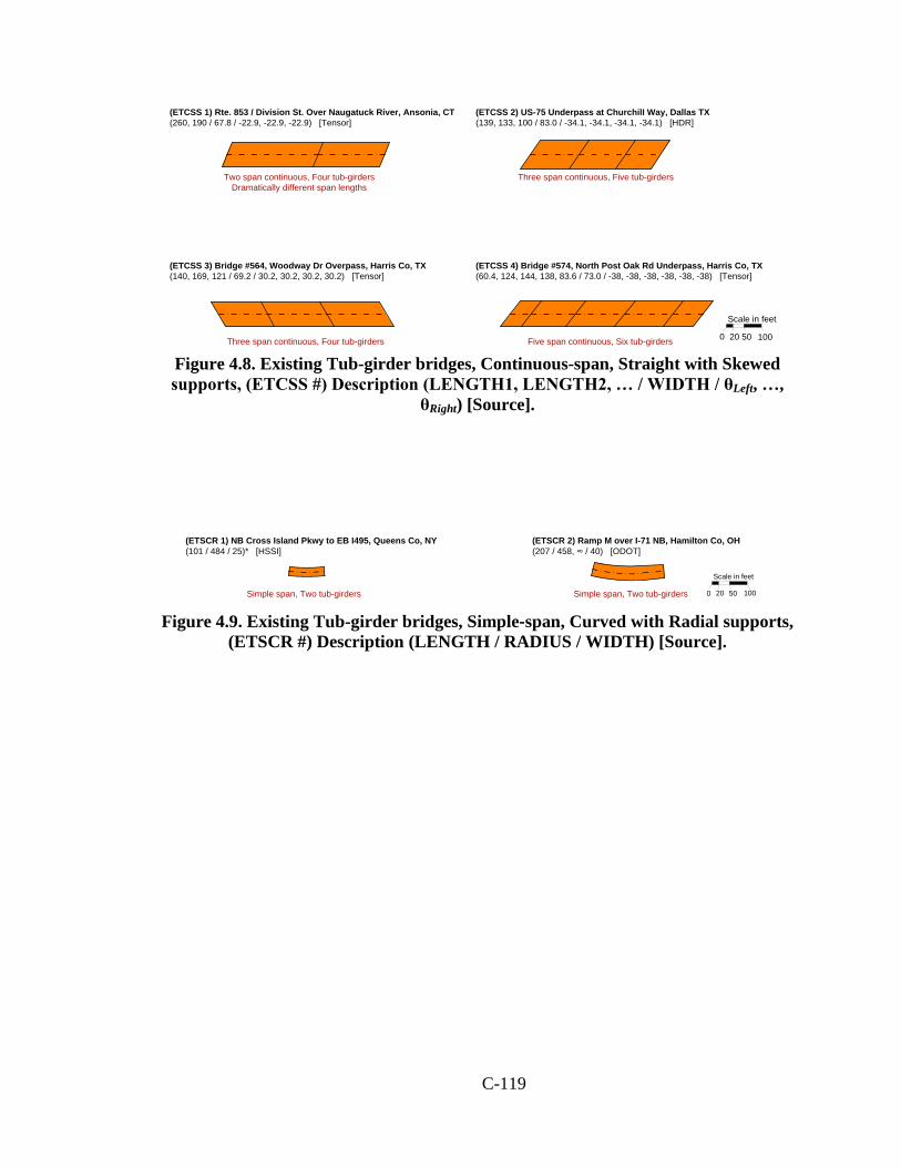
C-119

(ETCSS 2) US-75 Underpass at ChurchilI Way, Dallas TX(139, 133, 100 / 83.0 / -34.1, -34.1, -34.1, -34.1) [HDR]

Three span continuous, Five tub-girders

(ETCSS 1) Rte. 853 / Division St. Over Naugatuck River, Ansonia, CT(260, 190 / 67.8 / -22.9, -22.9, -22.9) [Tensor]

(ETCSS 4) Bridge #574, North Post Oak Rd Underpass, Harris Co, TX(60.4, 124, 144, 138, 83.6 / 73.0 / -38, -38, -38, -38, -38, -38) [Tensor]

(ETCSS 3) Bridge #564, Woodway Dr Overpass, Harris Co, TX(140, 169, 121 / 69.2 / 30.2, 30.2, 30.2, 30.2) [Tensor]

Five span continuous, Six tub-girdersThree span continuous, Four tub-girders

Two span continuous, Four tub-girdersDramatically different span lengths

Scale in feet

0 20 50 100

Figure 4.8. Existing Tub-girder bridges, Continuous-span, Straight with Skewed supports, (ETCSS #) Description (LENGTH1, LENGTH2, … / WIDTH / θLeft, …,

θRight) [Source].

(ETSCR 1) NB Cross Island Pkwy to EB I495, Queens Co, NY (101 / 484 / 25)* [HSSI]

Simple span, Two tub-girders

(ETSCR 2) Ramp M over I-71 NB, Hamilton Co, OH(207 / 458, ∞ / 40) [ODOT]

Simple span, Two tub-girders

Scale in feet

0 20 50 100

Figure 4.9. Existing Tub-girder bridges, Simple-span, Curved with Radial supports,

(ETSCR #) Description (LENGTH / RADIUS / WIDTH) [Source].

C-120

(ETCCR 4) NB Whitestone Expwy I-678 Spans 11-13, Queens Co, NY(213, 312, 199 / 416, ∞ / 42.4) [NYSDOT]

(ETCCR 3) NB Whitestone Expwy I-678 Spans 8-10, Queens Co, NY(155, 203, 157 / 416 / 42.4) [NYSDOT]

Three span continuous, Two tub-girders Three span continuous, Two tub-girders

(ETCCR 1) SB I-635 ramp over WB I-35 & BNSF RR to EB & WB I-35, Johnson Co, KS(69, 138, 80.5, 57.5 / 500 / 38.5) [KDOT]

Four span continuous, Three tub-girders

(ETCCR 2) US 119 over KY 1441 and Raccoon Creek, Pike Co, KY(247, 369, 356, 282 / ∞, 3246 / 45) and (247, 378, 364, 288 / ∞, 3316 / 45) [HSSI]

Four span continuous, Two independent bridges (two tub-girders each)

(ETCCR 6) Connector "K" over IH-35, Austin, TX (168, 242, 168 / 574 / 30) [TxDOT]

(ETCCR 5) Connector "Z", EB RM 2222 to SB IH-35, Austin, TX (151, 189, 150 / 447 / 30) [TxDOT]

Three span continuous, Two tub-girdersField data available (Chen 2002, Memberg 2002),

Studied by Topkaya et al.(2002)

Three span continuous, Two tub-girdersField data available (Cheplak 2001), Studied by Topkaya et al. (2002) Scale in feet

0 20 50 100 Figure 4.10. Existing Tub-girder bridges, Continuous-span, Curved with Radial

supports, (ETCCR #) Description (LENGTH1, LENGTH2, … / RADIUS1, RADIUS2, … / WIDTH) [Source].

C-121

(ETCCR 7) DC02 Spans 1&2 IH-30 PGBT Interchange, Dallas, TX(164, 164 / 895 / 29) [HDR]


(ETCCR 13) DC04 Spans 24, 25&26 IH-30 PGBT Interchange, Dallas, TX(204, 254, 204 / 2060 / 29) [HDR]

Two span continuous, Two tub-girders

Two span continuous, Two tub-girders Three span continuous, Two tub-girders

(ETCCR 10) DC03 Spans 1, 2&3 IH-30 PGBT Interchange, Dallas, TX(149, 189, 149 / 1010 / 29) [HDR]




Two span continuous, Two tub-girders Two span continuous, Two tub-girders

Two span continuous, Two tub-girdersThree span continuous, Two tub-girders

(ETCCR 14) Connector EB North Beltway 8 to NB I-45, Houston, TX(186, 286, 180 / 895 / 40.8) [TxDOT]

Three span continuous, Two tub-girdersField data available (Fan 1999)

Scale in feet

0 20 50 100

Figure 4.10. (continued). Existing Tub-girder bridges, Continuous-span, Curved with Radial supports, (ETCCR #) Description (LENGTH1, LENGTH2, … /

RADIUS1, RADIUS2, … / WIDTH) [Source].

C-122

(ETCCR 18) B-40-1321 Marquette Interchange, Milwaukee, WI(196, 242, 241, 176, 184, 184, 183, 101 / ∞, 1101 / 42.5)* [WisDOT]

(ETCCR 15) B-40-1122 Marquette Interchange, Milwaukee, WI(155, 169, 232, 185, 185, 144 / 515, 960, ∞, -1904 / 29.5)* [WisDOT]

(ETCCR 16) B-40-1131 Marquette Interchange, Milwaukee, WI(106, 212, 252, 191, 167 / 769, 960, ∞ / 29.5)* [WisDOT]

(ETCCR 17) B-40-1221 Unit 2 Marquette Interchange, Milwaukee, WI(171, 233, 233, 233, 209, 145 / 631, 949, ∞, -960 / 29.5)* [WisDOT]

Six span continuous, Two tub-girders

Five span continuous, Two tub-girders


Eight span continuous, Two tub-girders

(ETCCR 19) B-40-1421 Unit 2 Marquette Interchange, Milwaukee, WI(180, 180,180,179, 178, 125 / 642, 1151, ∞ / 29.9)* [WisDOT]

(ETCCR 20) B-40-1422 Unit 2 Marquette Interchange, Milwaukee, WI(150, 166, 167, 159, 159, 224, 227, 160 / ∞, 1150, 573, ∞ / 42.9)* [WisDOT]


Nine span continuous, Two tub-girders

Scale in feet

0 20 50 100

* Bridge has detailed erection plans. Figure 4.10. (continued). Existing Tub-girder bridges, Continuous-span, Curved

with Radial supports, (ETCCR #) Description (LENGTH1, LENGTH2, … / RADIUS1, RADIUS2, … / WIDTH) [Source].

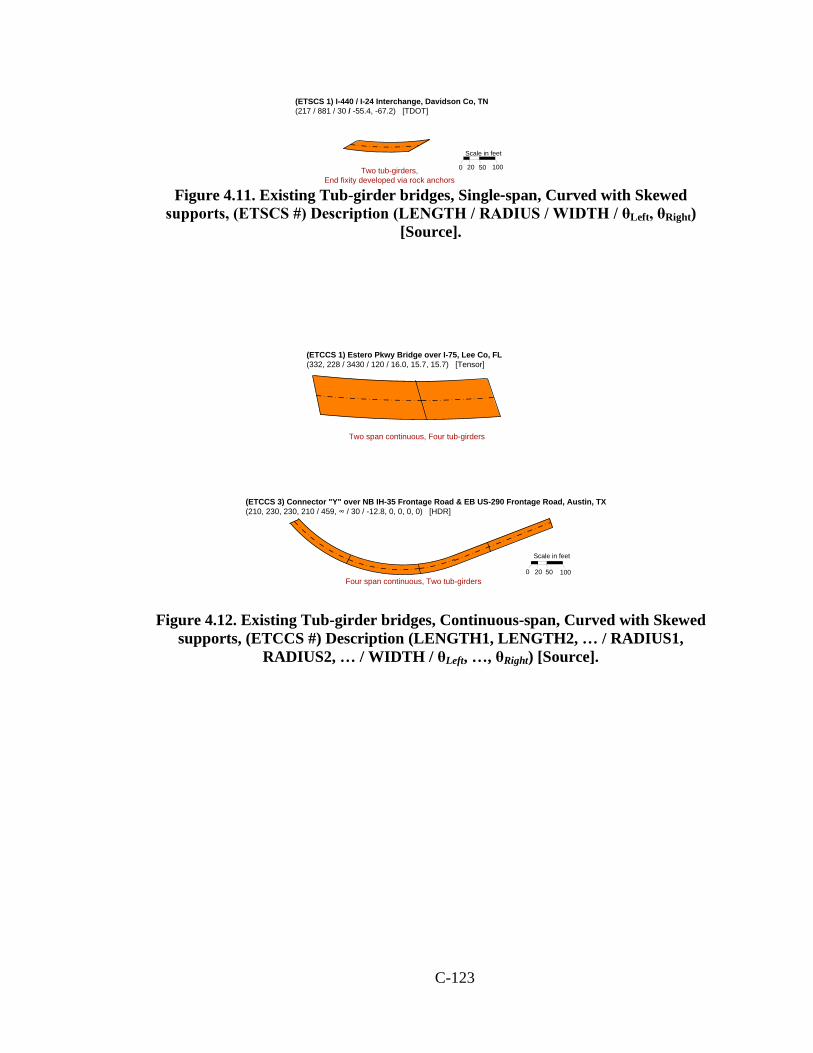
C-123

(ETSCS 1) I-440 / I-24 Interchange, Davidson Co, TN(217 / 881 / 30 / -55.4, -67.2) [TDOT]

Two tub-girders,End fixity developed via rock anchors

Scale in feet

0 20 50 100

Figure 4.11. Existing Tub-girder bridges, Single-span, Curved with Skewed

supports, (ETSCS #) Description (LENGTH / RADIUS / WIDTH / θLeft, θRight) [Source].

(ETCCS 3) Connector "Y" over NB IH-35 Frontage Road & EB US-290 Frontage Road, Austin, TX(210, 230, 230, 210 / 459, ∞ / 30 / -12.8, 0, 0, 0, 0) [HDR]

Four span continuous, Two tub-girders

(ETCCS 1) Estero Pkwy Bridge over I-75, Lee Co, FL(332, 228 / 3430 / 120 / 16.0, 15.7, 15.7) [Tensor]

Two span continuous, Four tub-girders

Scale in feet

0 20 50 100

Figure 4.12. Existing Tub-girder bridges, Continuous-span, Curved with Skewed

supports, (ETCCS #) Description (LENGTH1, LENGTH2, … / RADIUS1, RADIUS2, … / WIDTH / θLeft, …, θRight) [Source].

C-124

(ETCCS 4) Connector "T", EB Ben White Blvd to NB IH-35, Spans 14 to 22, Austin, TX(200, 270, 283, 168, 133, 274, 294, 215, 166 / 1660 / 28.4 / -7.53, 0, ..., 0, 8.97) [TxDOT]

Nine span continuous, Two tub-girdersField data available (Li 2004)

(ETCCS 6) SB Magruder Blvd to SB I-64, Hampton, VA(168, 193 / 801 / 25.3 / 0, -39.9, 0), (153, 220 / 827 / 25.3 / 0, -38.4, 0) [VDOT]

Two span continuous, Four tub-girdersPhased construction

Field observations availableFitup issues encountered during erection

(ETCCS 5 a) Ramp A2, SR 9A / SR 202 Interchange, Duval Co, FL(185, 164 / 765 / 30 / 0, -4.8, 0) [Tensor]

Two span continuous, Two tub-girders

Scale in feet

0 20 50 100

(ETCCS 7) WN-7 Ramp, Capitol Lake Interchange, Olympia ,WA( 217, 199 / 578 / 41 / -22.4, -51.8, -39.5 )

Two span continuous, Two tub-girdersCIP concrete end diaphragms

Figure 4.12. (continued). Existing Tub-girder bridges, Continuous-span, Curved

with Skewed supports, (ETCCS #) Description (LENGTH1, LENGTH2, … / RADIUS1, RADIUS2, … / WIDTH / θLeft, …, θRight) [Source].

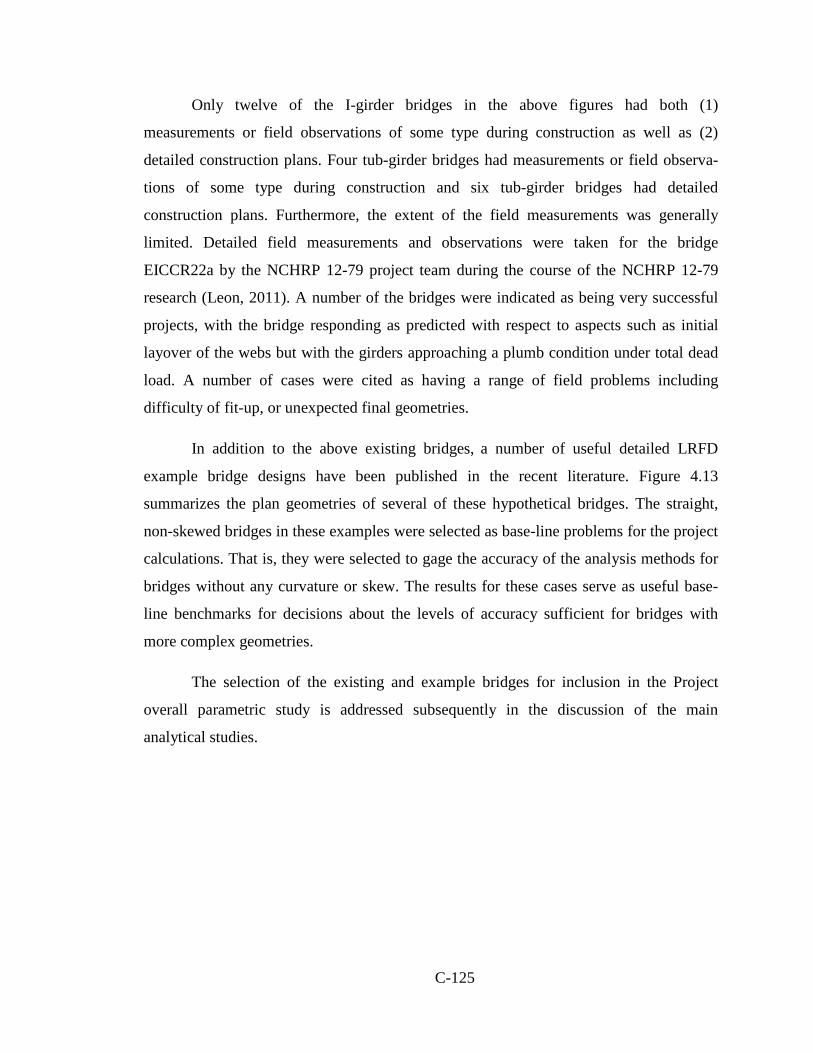
C-125

Only twelve of the I-girder bridges in the above figures had both (1)

measurements or field observations of some type during construction as well as (2)

detailed construction plans. Four tub-girder bridges had measurements or field observa-

tions of some type during construction and six tub-girder bridges had detailed

construction plans. Furthermore, the extent of the field measurements was generally

limited. Detailed field measurements and observations were taken for the bridge

EICCR22a by the NCHRP 12-79 project team during the course of the NCHRP 12-79

research (Leon, 2011). A number of the bridges were indicated as being very successful

projects, with the bridge responding as predicted with respect to aspects such as initial

layover of the webs but with the girders approaching a plumb condition under total dead

load. A number of cases were cited as having a range of field problems including

difficulty of fit-up, or unexpected final geometries.

In addition to the above existing bridges, a number of useful detailed LRFD

example bridge designs have been published in the recent literature. Figure 4.13

summarizes the plan geometries of several of these hypothetical bridges. The straight,

non-skewed bridges in these examples were selected as base-line problems for the project

calculations. That is, they were selected to gage the accuracy of the analysis methods for

bridges without any curvature or skew. The results for these cases serve as useful base-

line benchmarks for decisions about the levels of accuracy sufficient for bridges with

more complex geometries.

The selection of the existing and example bridges for inclusion in the Project

overall parametric study is addressed subsequently in the discussion of the main

analytical studies.

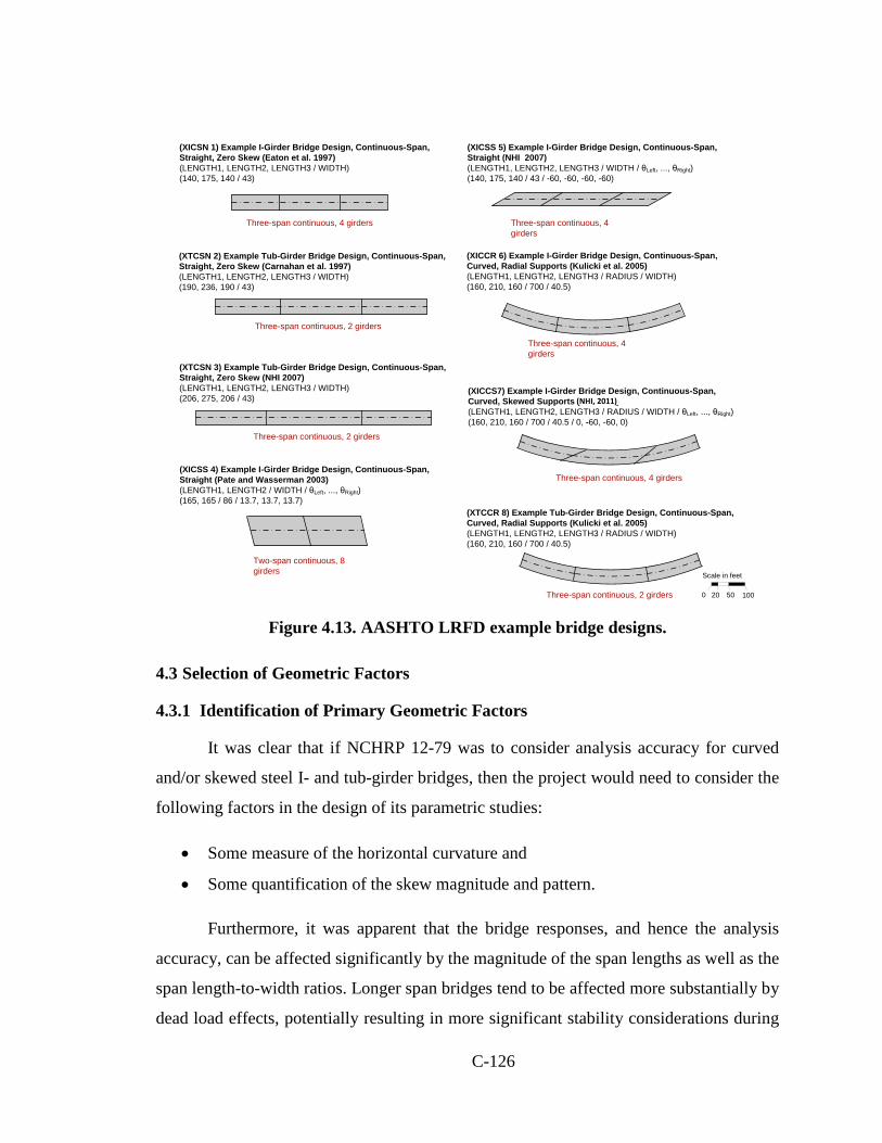
C-126


(XICSN 1) Example I-Girder Bridge Design, Continuous-Span, Straight, Zero Skew (Eaton et al. 1997)(LENGTH1, LENGTH2, LENGTH3 / WIDTH)(140, 175, 140 / 43)


(XTCSN 3) Example Tub-Girder Bridge Design, Continuous-Span, Straight, Zero Skew (NHI 2007)(LENGTH1, LENGTH2, LENGTH3 / WIDTH)(206, 275, 206 / 43)


(XTCSN 2) Example Tub-Girder Bridge Design, Continuous-Span, Straight, Zero Skew (Carnahan et al. 1997)(LENGTH1, LENGTH2, LENGTH3 / WIDTH)(190, 236, 190 / 43)

(XICSS 4) Example I-Girder Bridge Design, Continuous-Span, Straight (Pate and Wasserman 2003)(LENGTH1, LENGTH2 / WIDTH / θLeft, ..., θRight)(165, 165 / 86 / 13.7, 13.7, 13.7)


(XICCR 6) Example I-Girder Bridge Design, Continuous-Span, Curved, Radial Supports (Kulicki et al. 2005)(LENGTH1, LENGTH2, LENGTH3 / RADIUS / WIDTH)(160, 210, 160 / 700 / 40.5)


(XICSS 5) Example I-Girder Bridge Design, Continuous-Span, Straight (NHI 2007)(LENGTH1, LENGTH2, LENGTH3 / WIDTH / θLeft, ..., θRight)(140, 175, 140 / 43 / -60, -60, -60, -60)


(XICCS7) Example I-Girder Bridge Design, Continuous-Span, Curved, Skewed Supports (NHI 2009)(LENGTH1, LENGTH2, LENGTH3 / RADIUS / WIDTH / θLeft, ..., θRight)(160, 210, 160 / 700 / 40.5 / 0, -60, -60, 0)


Scale in feet

0 20 50 100

(XTCCR 8) Example Tub-Girder Bridge Design, Continuous-Span, Curved, Radial Supports (Kulicki et al. 2005)(LENGTH1, LENGTH2, LENGTH3 / RADIUS / WIDTH)(160, 210, 160 / 700 / 40.5)

Three-span continuous, 2 girders Figure 4.13. AASHTO LRFD example bridge designs.

4.3 Selection of Geometric Factors

4.3.1 Identification of Primary Geometric Factors

It was clear that if NCHRP 12-79 was to consider analysis accuracy for curved

and/or skewed steel I- and tub-girder bridges, then the project would need to consider the

following factors in the design of its parametric studies:

• Some measure of the horizontal curvature and

• Some quantification of the skew magnitude and pattern.

Furthermore, it was apparent that the bridge responses, and hence the analysis

accuracy, can be affected significantly by the magnitude of the span lengths as well as the

span length-to-width ratios. Longer span bridges tend to be affected more substantially by

dead load effects, potentially resulting in more significant stability considerations during

(NHI, 2011)

C-127

construction. In addition, beyond a certain span length, I-girder bridges are more likely to

need partial or full-span horizontal flange-level bracing systems to ensure adequate

stability and sufficient resistance to lateral loads during construction. Flange lateral

bracing systems cause portions of the structure to act as “pseudo-box girders,”

fundamentally changing the behavior of the structural system. Furthermore, longer

bridges generally exhibit larger overall deflections. These larger overall deflections can

lead to larger relative deflections at certain locations in the structural system, which can

sometimes be problematic during construction. Longer span bridges often have a smaller

ratio of the girder spacing relative to the girder depths, and typically have larger girder

depth-to-flange-width ratios. These attributes can fundamentally affect various relative

deflections in the structure as well as local and overall behavior and analysis accuracy at

the different stages of construction.

In addition, the bridge span length-to-width ratios can significantly impact the

influence of skew. Skewed bridges with smaller span length-to-width ratios tend to have

more significant load transfer to the bearing lines across the width of the structure, and

hence more significant “nuisance stiffness” effects that need to be addressed in the

design. Furthermore, relatively narrow horizontally curved bridges experience a greater

torsional “overturning component” of the reactions, which tends to increase the vertical

reactions on the girders further from the center of curvature and decrease the vertical

reactions on the girders closer to the center of curvature. In addition, relatively wide

horizontally-curved bridges can have more substantial concerns related to overturning at

intermediate stages of the steel erection, prior to assembly of the girders across the full

width of the bridge cross-section. These spans become more stable as additional girders

are erected and connected by cross-frames across the width of the bridge. Wide

horizontally-curved bridges also can have greater concerns associated with overturning

forces during deck placement.

Lastly, it was apparent that the bridge responses (and the analysis accuracy) can

be significantly affected by whether the spans are simply-supported or continuous.

Simple-span bridges tend to have larger deflections for a given geometry, and potentially

can be more difficult to handle during construction. Although simple-span girders can see

C-128

negative bending during erection (due to lifting or temporary support from holding

cranes, etc.), continuous-spans have more significant negative bending considerations.

Furthermore, particularly in I-girder bridges, continuous-span bridges can have

significant interactions between adjacent spans with respect to both major-axis bending

as well as the overall torsional response.

All of the above factors can have a substantial influence on the many detailed

structural attributes of steel I-girder and tub-girder bridges. Also, there can be significant

interactions between these factors in terms of their influence on the bridge responses, as

well as the accuracy of different bridge analysis methods.

If one considers the many detailed attributes of steel I- and tub-girder bridge

structural systems and their members and components addressed subsequently, the

combinations and permutations of potential bridge designs become endless. Hence, it was

decided that the most practical way of covering the design space of curved and/or skewed

I-girder and tub-girder bridges was to consider a range of practical combinations and

permutations of the following primary factors:

• Span length of the bridge centerline, Ls,

• Deck width normal to the girders, w, (in phased construction projects, w is

determined separately for each bridge unit)

• Horizontal curvature, of which the most appropriate characterization is discussed

below,

• Skew angle of the bearing lines relative to the bridge centerline, θ,

• Skew pattern of the bearing lines, of which the most appropriate characterization

is discussed below, and

• Span type, simple and various types of continuous-spans.

4.3.1.1 Characterization of Horizontal Curvature

The NCHRP 12-79 project team identified the torsion index, IT, discussed in

Section 3.1.4 as a useful measure of the degree of curvature of the bridge spans at an

early stage of the project. This parameter is closely related to the magnitude of the overall

torsion that exists in the bridge (or bridge unit).

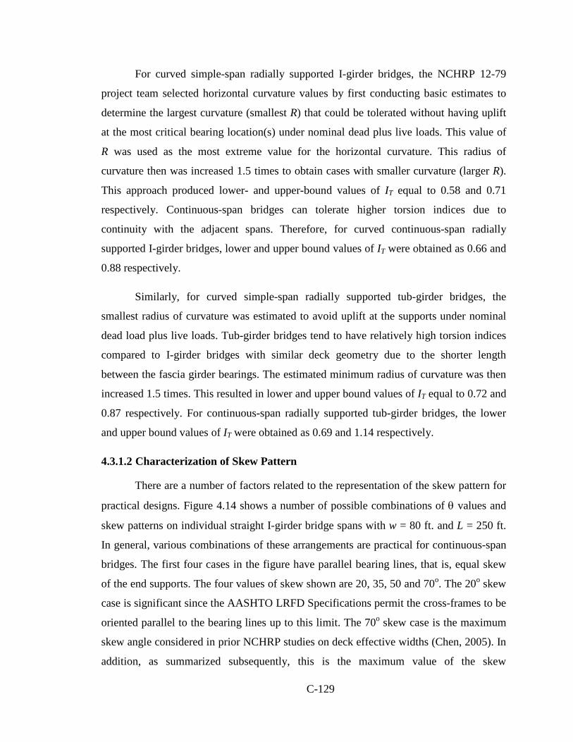
C-129

For curved simple-span radially supported I-girder bridges, the NCHRP 12-79

project team selected horizontal curvature values by first conducting basic estimates to

determine the largest curvature (smallest R) that could be tolerated without having uplift

at the most critical bearing location(s) under nominal dead plus live loads. This value of

R was used as the most extreme value for the horizontal curvature. This radius of

curvature then was increased 1.5 times to obtain cases with smaller curvature (larger R).

This approach produced lower- and upper-bound values of IT equal to 0.58 and 0.71

respectively. Continuous-span bridges can tolerate higher torsion indices due to

continuity with the adjacent spans. Therefore, for curved continuous-span radially

supported I-girder bridges, lower and upper bound values of IT were obtained as 0.66 and

0.88 respectively.

Similarly, for curved simple-span radially supported tub-girder bridges, the

smallest radius of curvature was estimated to avoid uplift at the supports under nominal

dead load plus live loads. Tub-girder bridges tend to have relatively high torsion indices

compared to I-girder bridges with similar deck geometry due to the shorter length

between the fascia girder bearings. The estimated minimum radius of curvature was then

increased 1.5 times. This resulted in lower and upper bound values of IT equal to 0.72 and

0.87 respectively. For continuous-span radially supported tub-girder bridges, the lower

and upper bound values of IT were obtained as 0.69 and 1.14 respectively.

4.3.1.2 Characterization of Skew Pattern

There are a number of factors related to the representation of the skew pattern for

practical designs. Figure 4.14 shows a number of possible combinations of θ values and

skew patterns on individual straight I-girder bridge spans with w = 80 ft. and L = 250 ft.

In general, various combinations of these arrangements are practical for continuous-span

bridges. The first four cases in the figure have parallel bearing lines, that is, equal skew

of the end supports. The four values of skew shown are 20, 35, 50 and 70o. The 20o skew

case is significant since the AASHTO LRFD Specifications permit the cross-frames to be

oriented parallel to the bearing lines up to this limit. The 70o skew case is the maximum

skew angle considered in prior NCHRP studies on deck effective widths (Chen, 2005). In

addition, as summarized subsequently, this is the maximum value of the skew

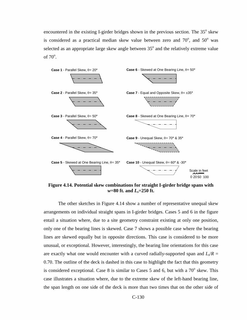
C-130

encountered in the existing I-girder bridges shown in the previous section. The 35o skew

is considered as a practical median skew value between zero and 70o, and 50o was

selected as an appropriate large skew angle between 35o and the relatively extreme value

of 70o.

Case 1 - Parallel Skew, θ= 20°

Scale in feet

0 20 50 100




Case 5 - Skewed at One Bearing Line, θ= 35°


Case 10 - Unequal Skew, θ= 60° & -30°

Case 7 - Equal and Opposite Skew, θ= ±35°


Case 9 - Unequal Skew, θ= 70° & 35°

Figure 4.14. Potential skew combinations for straight I-girder bridge spans with

w=80 ft. and Ls=250 ft.

The other sketches in Figure 4.14 show a number of representative unequal skew

arrangements on individual straight spans in I-girder bridges. Cases 5 and 6 in the figure

entail a situation where, due to a site geometry constraint existing at only one position,

only one of the bearing lines is skewed. Case 7 shows a possible case where the bearing

lines are skewed equally but in opposite directions. This case is considered to be more

unusual, or exceptional. However, interestingly, the bearing line orientations for this case

are exactly what one would encounter with a curved radially-supported span and Ls/R =

0.70. The outline of the deck is dashed in this case to highlight the fact that this geometry

is considered exceptional. Case 8 is similar to Cases 5 and 6, but with a 70o skew. This

case illustrates a situation where, due to the extreme skew of the left-hand bearing line,

the span length on one side of the deck is more than two times that on the other side of

C-131

the deck, i.e., L2/L1 > 2. A value of L2/L1 = 2 was considered to be a practical maximum

limit by the NCHRP 12-79 project team. It should be noted that if the span length of the

centerline were larger, or if the deck width w were smaller for this case, this L2/L1 limit

would not be exceeded. The outline of the deck geometry for Case 8 is shown as a grey

line and the deck plan is shaded white to emphasize that this deck geometry is considered

impractical. The above L2/L1 limit can be satisfied with θ = 70o if the bearing lines are

parallel as in Case 4, or if the bearing lines are unequally skewed such as in Case 9.

Lastly, Case 10 shows an extreme situation of unequal skew in opposite directions for the

two bearing lines. In this case, the bearing lines are oriented at 90o relative to one

another. The project team decided that one would practically never encounter a relative

angle between adjacent bearing lines of more than 90o. This type of bearing arrangement

could occur for example if the span were crossing the corner of a rectangular lot and the

bearing lines had to be placed parallel to the sides of the lot. Note that L2/L1 > 2 for Case

10; however, if the span is larger or the deck width is smaller, the L2/L1 < 2 limit could be

satisfied.

The skew arrangements on straight tub-girder bridges can be similar to those

considered in Figure 4.14. However, tub-girder bridges generally tend to have smaller

skew values, due to the expected sensitivity of these types of bridges to skew effects as

well as the fabrication difficulties and increased cost associated with complex skewed

diaphragm connection details.

Figure 4.15 shows the various possible combinations of horizontal curvature and

approximately + 15 and 30o skew on individual tub-girder bridge spans with Ls = 150 ft.,

w = 30 ft. and R = 400 ft. Again, various combinations of these arrangements are possible

for continuous-span bridges. The skew and horizontal curvature combinations in Figure

4.15 are similar to those shown for the straight bridge spans in Figure 4.14. However,

whereas a number of patterns with positive and negative skew produce the same net

geometry in straight bridges, these positive and negative skew values give different

geometries in similar curved bridges, due to the horizontal curvature. Fourteen total

combinations are shown in Figure 4.15 that need to be considered in general. A large

number of these combinations may be considered as exceptional cases and are drawn

C-132

with dashed lines. Note that for Cases 2, 5 and 9 in Figure 4.15, the magnitudes of the

skew angles are modified slightly to make the bearing lines parallel.

Case 11 θ=30,30

Case 8 θ=-30,-15

Case 4 θ=-30,0

Case 13 θ=-15,30

Case 14 θ=-30,30

Case 9 θ=30,8.5

Case 7 θ=-15,-15

Case 3 θ=-15,0 Case 10 θ=-15,15

Case 2 θ=21.5,0

Case 1 θ=15,0

Case 6 θ=30,-15

Case 5 θ=10.7,-10.7 Case 12 θ=30,-30

Parallel

Parallel Parallel

Figure 4.15. Example potential skew and horizontal curvature combinations for

curved tub-girder bridge spans with w = 30 ft., Ls = 150 ft. and R = 400 ft.

The possible combinations of skew and horizontal curvature for I-girder bridges

are similar to those shown in Figure 4.15, except that as noted previously, somewhat

larger skew values can be accommodated generally in I-girder bridges. However, the

extent of these patterns is limited by:

• A maximum limit on the ratio of the span lengths of the outside and inside edges

of the deck, Lso/Lsi, of 2, and

• A maximum limit on the orientation of adjacent bearing lines of 90o

C-133

similar to the limits discussed previously for the straight skewed bridges. Lastly, for

highly-curved spans, the Project team recognized that the skew angle at the inside edge of

the deck can be substantially larger than that at the deck centerline. This is illustrated by

Figure 4.16. It was decided that it is not practical for the skew angle at the inside edge of

the deck to be greater than 70o in these cases.

Figure 4.16. Highly-curved span with a skew angle of 70° at the inside edge of the

deck and 54.9o at the centerline of the deck, w = 80 ft., Ls = 150 ft., R = 308 ft.

All of the above factors can have a substantial influence on the many detailed

structural attributes of steel I-girder and tub-girder bridges. Also, there can be significant

interactions between these factors in terms of their influence on the bridge responses, as

well as the accuracy of different bridge analysis methods.

4.3.2 Synthesis of Primary Factor Ranges from the Collected Bridges

Upon synthesis of the primary factors from the existing bridges collected by

NCHRP 12-79, the following ranges of these factors were observed:

• Span length, Ls o I-Girder

120 to 254 ft. (straight simple-spans with skewed supports) 90 ft. (curved simple-spans with radial supports) Only one bridge was identified as curved simple-span with radial supports; this was the FHWA Test bridge, EISCR1. 106 to 252 ft. (curved simple-spans with skewed supports) 119 to 445 ft. (straight continuous-spans with zero skew) 73 to 257 ft. (straight continuous-spans with skewed supports) 101 to 334 ft. (curved continuous-spans with radial supports) 50 to 279 ft. (curved continuous-spans with skewed supports)

θright = 54.9o

θmax = 70o

θleft = 27.0o

ParallelScale in feet

0 20 50 100

C-134

o Tub-Girder 139 to 205 ft. (straight simple-spans with skewed supports)

101 to 207 ft. (curved simple-spans with radial supports) 217 ft. (curved simple-spans with skewed supports) Only one bridge was identified as curved simple-span with skewed supports; this was the bridge ETSCS1. 57.5 to 373 ft. (curved continuous-spans with radial supports) 153 to 332 ft. (curved continuous-spans with skewed supports)

• Deck width (per unit in cases involving phased construction), w o I-Girder

24 to 87.5 ft. (spans with skew) 30 to 71 ft. (spans with radial supports, with the exception of the EISCR1 FHWA test bridge, which was 23.5 ft.)

o Tub-Girder 25 to 45 ft. (spans with two tub-girders)

36 ft. to 120 ft. (spans with more than two tub-girders) • Torsion Index, IT

o I-Girder 0.48 to 0.87

o Tub-Girder 0.50 to 1.14 (spans with two tub-girders; an IT larger than 1.0 is possible due to

continuity with adjacent spans) 0.50 to 0.84 (spans with more than two tub-girders)

• Skew angle of the bearing lines relative to a tangent to the bridge centerline, θ o I-Girder

0 to 69.5o (straight bridges) 0 to 64.3o (curved bridges)

o Tub-Girder

0 to 12.8o (spans with two tub-girders, excluding the ETCCS7 bridge, which had CIP concrete end diaphragms and non-typical bearing details) 0 to 38.9o (spans with more than two tub-girders)

• Skew pattern o I-Girder

The bearing lines were parallel in most of the collected I-girder bridges. One straight bridge (EICSS2) has θ = 61.8o & 38o in one span. One curved bridge (EICCS15) has θ = 0o & 49.5o resulting in a 19.8o differ-ence in orientation between the bearing lines in one span. One curved bridge (EICCS5) has θ = 0o & 60.2o resulting in a 72o difference in orientation between the bearing lines in one span.

C-135

o Tub-Girder All the skewed spans have non-parallel bearing lines for the collected bridges that are

composed of two tub-girders. One curved bridge with two tub-girders (ETCCS3) has θ = 0o & 12.8o and a 39.0o difference in orientation between the bearing lines. One curved bridge with two tub-girders (ETCCS7) has θ = 51.8o & 39.5o and a 32.0o difference in orientation between the bearing lines; however, this bridge has cast-in-place (CIP) concrete end diaphragms and non-typical bearing details. Most of the skewed spans with more than two tub-girders have parallel bearing lines. One two-span continuous curved bridge with four tub-girders (ETCCS6), constructed in two phases with two girders in each phase, has θ = 0o & 38.9o and a difference in orientation of 53.8o between the bearing lines in one span. However, no cross-frames or diaphragms are placed between the girders at the interior bearing line on this bridge, and this bridge does not contain any internal intermediate cross-frames or diaphragms.

• Type-of-span o I-Girder

Most of the collected I-girder bridges are continuous-span. Ratio of exterior-to-interior span lengths: 0.56 to 1.25 Ratio of adjacent interior span lengths: 0.63 to 1.0 Ratio of span lengths, 2-span continuous: 0.77 to 1.0

o Tub-Girder Most of the collected tub-girder bridges are continuous-span.

Ratio of exterior-to-interior span lengths: 0.49 to 1.0 Ratio of adjacent interior span lengths: 0.49 to 1.0 Ratio of span lengths, 2-span continuous: 0.69 to 1.0 A fraction of the bridges with more than two tub-girders are simple-span.

The values for several additional “secondary” parameters discussed in the above, but not

selected as primary factors were:

• Span length to deck width ratio, Ls/w (per unit in phased construction jobs) o I-Girder

0.55 to 14.77 (spans with skew) 1.67 to 8.83 (curved spans with radial supports)

o Tub-Girder 2.80 to 8.76 (radially-supported spans with two tub-girders)

4.66 to 10.35 (skewed spans with two tub-girders) 0.83 to 3.83 (skewed spans with more than two tub-girders)

• Subtended angle of the span’s centerline, Ls/R o I-Girder

0.0 to 0.57 radians (32.6o) o Tub-Girder

C-136

0.0 to 0.68 radians (39.0o) (spans with two tub-girders) 0.07 to 0.28 radians (16.0o) (spans with more than two tub-girders)

In addition to the above parameters, several additional key indices that correlate with the

accuracy of different simplified analysis methods were identified during the course of the

NCHRP 12-79 research. These indices are discussed in Chapter 3. The ranges of values

among the collected bridges for these indices are as follows.

• Skew index, IS o I-Girder

0.05 to 1.93 o Tub-Girder

0.08 to 0.77 (spans with two tub-girders) 0.01 to 0.18 (spans with more than two tub-girders) • Connectivity index, IC


o Tub-Girder The connectivity index is not applicable to tub-girder bridges • Girder length index, IL


o Tub-Girder 1.0 to 1.09

4.3.3 Selection of Primary Factor Ranges and Levels

Table 4.1 shows the ranges and levels of the primary factors that were selected for

the main analytical study of NCHRP 12-79. These primary factors are discussed in detail

in the preceding sections.

The first row of Table 4.1 addresses the type of span. This factor is addressed in a

similar fashion for both the I- and tub-girder bridges. Three-span continuous designs with

one balanced end span and one end span of equal length to the main span capture both the

behavior associated with drop-in spans as well as the interactions between balanced and

unbalanced continuous-spans. However, two-span continuous bridges are apt to be more

sensitive to skew effects. Also, the potential combinations of skew arrangements become

large as the number of spans is increased. Many of these combinations would have a

minor effect on the final analysis accuracy assessments though, due to the fact that the

C-137

influence of the skew at a particular bearing line tends to die out as one moves several

spans away from this bearing line. Furthermore, long multi-span curved bridges often

may have only a few skewed bearing lines because of geometry constraints at a particular

location, whereas it may be possible to orient other bearing lines radially. This can be

understood by considering cases such as EICCS1 and EICCS5 in Figure 4.6. In these

structures, one would quickly reach the maximum practical θ value of approximately 70o

if, for instance, all the bearing lines were parallel.

It was desired to study several continuous-span bridges that had significant

unbalanced span lengths. This consideration was addressed by inserting selected existing

bridges into the matrix of parametric study bridges. Also, bridges with more than three

spans were considered by insertion of a number of existing bridges into the overall

parametric study matrix.

The second row of Table 4.1 shows the values selected for the span length. For

both I- and tub-girder bridges, the selected lengths for simple-spans were 150, 225 and

300 ft. and the selected lengths for continuous-spans were 150, 250 and 350 ft. The

maximum span length of Ls = 350 ft. was selected to match the maximum value targeted

by the AASHTO (2010) Specifications. All but one span of one of the existing I-girder

bridges had span lengths smaller than 350 ft., although three of the existing I-girder

bridge units had spans larger than 300 ft. The span larger than 350 ft. is one of the

straight spans of the Ford City bridge (EICCR 11). In current (2012) practice, horizontal

flange lateral bracing systems often are considered for span lengths of 250 ft. or more,

but spans of 250 ft. may be acceptable without flange level lateral bracing systems in

certain cases. A span length of Ls = 150 ft. is a rough lower-bound value at which welded

girders are generally required.

C-138

Table 4.1. Primary factor ranges and levels for the NCHRP 12-79 main analytical study.

Factor I-girder bridges Tub-girder bridges

Type of span

Simple, 2-span continuous, and 3-span continuous with one balanced end span and one end span equal in length to the main center span.

Use the above 3-span continuous bridges as base ICCR & TCCR cases.

Consider both 2- and 3-span continuous bridges for the ICSS and TCSS.

Consider only 2-span continuous cases for the ICCS and TCCS designs.

Consider at least one 2-span continuous bridge with a significant unbalance between the span lengths.

Maximum span length of bridge centerline, Ls

150, 225 & 300 ft. for simple-spans

150, 250 & 350 ft. for continuous-spans

(measured along the curve)

Deck width, w

30 ft. (1 to 2 traffic lanes + shoulders & barriers)

80 ft. (4 to 5 traffic lanes + shoulders & barriers

30 ft. (1 to 2 traffic lanes + shoulders & barriers)

Torsion Index, IT

0.58 to 0.71 for ISCR bridges

0.66 to 0.88 for ICCR bridges

0.72 to 0.87 for TSCR bridges

0.69 to 1.14 for TCCR bridges

Skew angle relative to the bridge centerline, θ

20o, 35o, 50o & 700 but with θ at the inside edge of the

deck < 70o in curved spans

15o & 30o, plus additional sensitivity studies with variations

up to ±15° from zero skew

Skew pattern

Consider the + combinations of skew angles shown in Figure 4.14 (for straight bridges) and Figure 4.15 (for curved bridges), but using θ = 35

& 70o for I-girder bridges and θ = 15 & 30o for tub-girder bridges. Limit the ratio of the span lengths along the edges of the deck, L2/L1, to

a maximum value of 2.0 in all cases.

Limit the difference in orientation of adjacent bearing lines to a maximum of 90o in all cases.

Give preference to typical (i.e., non-exceptional) bridge geometries.

C-139

Of the existing tub-girder bridges, only the two interior spans of the parallel US

119 bridges over KY 1441 and Raccoon Creek in Pike Co., KY (bridge ETCCR 2) have

span lengths greater than 350 ft., although there are two other tub-girder bridges with

spans larger than 300 ft.

The third row of Table 4.1 shows the selected deck widths for the parametric

study bridges. For the I-girder bridge parametric designs, deck widths of 30 ft. and 80 ft.

were selected by the project team. Only 30 ft. deck widths were considered in the new

parametric designs for the tub-girder bridges. This smaller 30 ft. width is representative

of one- to two-lane bridges, whereas the larger 80 ft. width is representative of structures

with four to five lanes. A large number of the existing tub-girder bridges are one to two

lane ramp type structures. Therefore, it was recommended that the Project should focus

predominantly on these types of structures in its studies of tub-girder bridge system

behavior and analysis accuracy. The less common tub-girder bridges having more than

two girders were addressed by including one of these existing bridge cases in the overall

parametric study matrix. However, this bridge involved phased construction, with each of

the phases having two tub girders.

The combinations of Ls from 150 to 350 ft. with w from 30 to 80 ft. give span

length to the bridge width, Ls/w, ranging from 150/80 = 1.88 to 350/30 = 11.7. The

maximum value for this range is slightly larger than the maximum Ls/w of 7.90 and 8.29

for the existing I- and tub-girder bridges. It was believed that these larger values should

be studied to fully address the bridge responses and analysis accuracies for these practical

but more extreme geometry conditions.

The fourth row of Table 4.1 gives the selected ranges and levels for the torsion

index IT. The implications of IT ranging from 0.5 to 1.0 have been discussed in Section

3.1.4. This parameter was used in establishing the horizontal radius of curvature R for the

ISCR/TSCR and ICCR/TCCR designs, given the span length Ls and the deck width w.

The horizontal radius of curvature obtained for the ISCR/TSCR designs was then

employed for other new curved ISCS/TSCS parametric bridge designs. Similarly, the

horizontal radius of curvature obtained for the ICCR/TCCR designs was employed for

the other new curved ICCS/TCCS parametric bridge designs. A maximum limit on Ls/R

C-140

of 1.0 was imposed on the parametric designs. This limit can govern for shorter spans

with wide decks and is somewhat larger than the maximum Ls/R of 0.57 and 0.68 radians

for the collected existing I- and twin tub-girder bridges. Nevertheless, it was believed that

Ls/R = 1.0 is a practical extreme that should be addressed in the parametric study design.

Wide bridges with these larger Ls/R values may require special handling during the steel

erection and/or deck placement.

The fifth row of Table 4.1 shows the selected ranges and levels of the skew angle

θ. As noted previously, AASHTO (2010) allows the cross-frames to be framed parallel to

the bearing lines in I-girder bridges with θ < 20o. Furthermore, it was expected that the

effects of skew may be sufficiently small such that a line girder analysis may work quite

adequately for certain cases at this skew level. A value of 70o is a reasonable maximum

limit for θ in I-girder bridges. This value was the maximum considered in studies of deck

effective widths by Chen (2005), and represents roughly the largest skew angle

encountered in the existing bridges. Smaller skew angles of 15 and 30o were targeted for

the tub-girder parametric study designs. In addition, a range of skew angles of +15o from

zero skew were considered in separate 3D FEA studies (with no separate consideration of

the simplified analysis methods) to understand the influence of skew on the tub-girder

bridge responses in greater detail.

Lastly, the sixth row of Table 4.1 explains the recommended variations of the

skew pattern considered. These variations are understood most easily by viewing the

actual deck plan geometries for various hypothetical new bridge designs. The reader is

referred to Section 4.3.4 for these illustrations.

4.3.4 Selection of the Analytical Study Bridges

The following sub-sections summarize the key characteristics of the I- and tub-

girder bridges selected for the NCHRP 12-79 analytical studies, given the ranges and

levels of the primary factors identified in Section 4.3.3. To arrive at the analytical study

design, the research team first developed a full factorial design matrix involving all the

above factors and levels. This led to more than 500 I-girder bridges and more than 250

tub-girder bridges that would need to be studied. Fortunately, a number of these

C-141

combinations and permutations could be considered impractical or unbuildable.

However, even after the impractical and unbuildable cases were eliminated, the total

number of bridges arrived at in the study design was relatively large. Therefore, some

prioritization of the bridges was necessary within the full range of practical designs. As

noted by Montgomery (2004), “If the experimenter can reasonably assume that certain

high-order interactions are negligible, information on the main effects and low-order

interactions may be obtained by running only a fraction of the complete factorial

experiment. These fractional factorial designs are among the most widely used types of

designs for product and process design and for process improvement.” In the context of

the Project 12-79 analytical study design, this involved the elimination of individual

bridges or groups of bridges where the interaction between the primary factor effects was

expected to be relatively small. Furthermore, a number of bridges in which the

combination of factors led to:

• Exceptional (i.e., particularly unusual) structures, or

• Designs that were very similar in one or more characteristics to other designs

were eliminated.

Once these selections were completed, the library of existing bridges summarized

in Figures 4.1 through 4.12 was searched for bridges that:

• Matched closely with the analytical study design selections, and

• Satisfied the criteria described in Section 4.1.

In a few cases, modifications were made to the analytical study design to include existing

bridges that were particularly good candidates based on the criteria specified in Section

4.1. In addition, several of the Example bridges from Figure 4.13 that matched closely

with the analytical study design selections were selected for inclusion in the analytical

study. The remaining bridges in the study design were targeted as “New” bridges,

indicating that they were to be fully designed by the project team using the AASHTO

LRFD Specifications and current common standards of care.

C-142

The initial design of the suite of bridges arrived at, based on the above process,

involved approximately 100 bridges. The bridges were then subdivided into smaller

suites for execution of the analytical studies. Various milestones were identified at which

the study bridge selections were reevaluated based on what was learned from the

completed studies. The resulting final study targeted 58 I-girder bridges and 18 tub-girder

bridges in total.

The following sections first discuss several base straight, non-skewed study

bridges considered at the beginning of the Project, followed by straight skewed simple

and continuous-span cases, then simple and continuous-span curved bridges with radial

supports, and finally curved and skewed simple- and continuous-span bridges. Each of

these sections includes summary sketches of the bridge deck plans and bearing-line

geometries corresponding to the designs along with a title block for each of the bridges

containing:

1) An identification label, composed of the letter “X” for the “eXample” bridge

designs, followed by the symbols explained at the beginning of Section 4.2,

indicating the bridge category (e.g., ISSS, ICSS, etc.), and ending with the bridge

number for that category. Two additional categories, ICSN and TCSN, are

introduced in Figure 4.17. The “CSN” designation stands for Continuous-span,

Straight, with Non-skewed supports. For example, the first eXample bridge in

Figure 4.17 is labeled “XICSN 1.”

2) An identification label, composed of the letter “E” for the “Existing” bridges,

followed by the above symbols indicating the bridge category, and ending with

the bridge number for that category, e.g., bridge “EISSS 3” in Figure 4.18.

3) An identification label, composed of the letter “N” for the “New” bridge designs,

followed by the above symbols indicating the bridge category, and ending with

the bridge number for that category, e.g., bridge “NISSS 1” in Figure 4.18.

4) A summary of the basic geometry information about the bridge, enclosed in

parentheses. For instance, in Figure 4.18, the basic geometry information

includes:

C-143

• The span length of the bridge centerline,

• The out-to-out width of the bridge deck perpendicular to the bridge centerline

(provided for each unit in phased construction jobs), and

• The skew angle with respect to centerline of the bridge for both bearing lines.

This information is conveyed symbolically in the figure caption as

“(LENGTH/WIDTH/θ1, θ2).” The other categories have similar but different

basic geometry information. This information is summarized symbolically in each

of the figure captions. The skew angle of the bearing lines is represented by the

symbol θ. This angle is taken as zero when a bearing line is perpendicular to the

centerline of the structure, that is, when the bearing line does not have any skew.

All of the figures referenced in the following sub-sections adopt the following

conventions:

• Typical or common geometries are sketched using a solid black outline,

• Geometries considered unusual or exceptional are sketched using a black dashed

outline,

• A few bridge geometries that are considered impractical or unbuildable are

sketched using a solid light-grey outline. (The only cases shown that are

impractical or unbuildable are a few bridges with high skew and relatively small

length-to-width ratios, where if the bridge span was longer or the deck was

narrower, the geometry would indeed be possible.)

• The deck plans for the selected eXample bridges are shaded and cross-hatched,

• The deck plans for the selected Existing bridges are shaded with a textured

background,

• The deck plans for the selected New bridges are shaded with a solid background,

• The deck plans of bridges that were not selected for study are white or unshaded,

• The bridge unit centerlines are indicated by a “dot-dash” line, and

• The different phases in phased construction bridges (i.e., bridges constructed as a

number of separate longitudinal units) are delineated by dashed lines.

C-144

4.3.4.1 Straight Non-skewed Base-Line Comparison Cases (XITSN 1 and XTCSN 3)

The straight non-skewed “base-line” bridges are illustrated in Figure 4.17. The

analysis accuracy results for these cases serve as useful indicators or benchmarks for

decisions about the levels of accuracy sufficient for bridges with more complex

geometries. Both of these bridges are carefully documented example designs.


(XICSN 1) Example I-Girder Bridge Design, Continuous-Span, Straight, Zero Skew (Eaton et al. 1997)(LENGTH1, LENGTH2, LENGTH3 / WIDTH)(140, 175, 140 / 43)


(XTCSN 3) Example Tub-Girder Bridge Design, Continuous-Span, Straight, Zero Skew (NHI 2007)(LENGTH1, LENGTH2, LENGTH3 / WIDTH)(206, 275, 206 / 43)

Scale in feet

0 20 50 100 Figure 4.17. eXample Straight Non-skewed bridges used as base comparison cases,

(LENGTH1, LENGTH2, LENGTH3 / WIDTH).

4.3.4.2 Simple-Span Bridges, Straight, with Skewed Supports (ISSS and TSSS)

Figure 4.18 shows the 60 total combinations and permutations for the ISSS bridges

obtained considering:

• The ten combinations of skew magnitude and pattern for the straight bridges

illustrated previously in Figure 4.14, {(θLeft, θRight ) = (20o,20o), (35o,35o),

(50o,50o), (70o,70o), (35o,0o), (50o,0o), (35o,-35o), (70o,0o), (70o,35o), (60 o,-30 o)},

• The three values for the length Ls (Ls = 150, 225 and 300 ft.), and

• The two values for the deck width w (w = 30 and 80 ft.)

C-145

NIS

SS 1

(150

/30/

20,2

0)N

ISSS

11

(150

/80/

20,2

0)N

ISSS

21

(225

/30/

20,2

0)N

ISSS

31

(225

/80/

20,2

0)N

ISSS

41

(300

/30/

20,2

0)N

ISSS

51

(300

/80/

20,2

0)

NIS

SS 2

(150

/30/

35,3

5)N

ISSS

12

(150

/80/

35,3

5)N

ISSS

22

( 225

/30/

35,3

5)N

ISSS

32

(225

/80/

35,3

5)N

ISSS

42

(300

/30/

35,3

5)

NIS

SS 4

(150

/30/

70,7

0)N

ISSS

24

(225

/30/

70,7

0)N

ISSS

44

(300

/30/

70,7

0)N

ISSS

54

(300

/80/

70,7

0)

NIS

SS 5

(150

/30/

35,0

)N

ISSS

15

(150

/80/

35,0

)N

ISSS

25

(225

/30/

35,0

)N

ISSS

35

(225

/80/

35,0

)N

ISSS

45

(300

/30/

35,0

)

NIS

SS 7

(150

/30/

35,-3

5)N

ISSS

17

(150

/80/

35,-3

5)N

ISSS

27

(225

/30/

35,-3

5)N

ISSS

37

( 225

/80/

28.6

,-28.

6)N

ISSS

47

(300

/30/

35,-3

5)N

ISSS

57

(300

/80/

35,-3

5)

NIS

SS 8

(150

/30/

70,0

)N

ISSS

18

(150

/80/

70,0

)N

ISSS

28

(225

/30/

70,0

)N

ISSS

38

(225

/80/

70,0

)N

ISSS

48

(300

/30/

70,0

)N

ISSS

58

(300

/80/

70,0

)

NIS

SS 9

(150

/30/

70,3

5)N

ISSS

19

(150

/80/

70,3

5)N

ISSS

29

(225

/30/

70,3

5)N

ISSS

39

(225

/80/

70,3

5)N

ISSS

49

(300

/30/

70,3

5)N

ISSS

59

(300

/80/

70,3

5)

NIS

SS 1

0 (1

50/3

0/60

,-30)

NIS

SS 2

0 (1

50/8

0/60

,-30)

NIS

SS 3

0 (2

25/ 3

0/60

,-30)

NIS

SS 4

0 (2

25/8

0/60

,-30)

NIS

SS 5

0 (3

00/3

0/60

,-30)

NIS

SS 6

0 (3

00/8

0/60

,-30)

Perp

endi

cula

rPe

rpen

dicu

lar

L2/L

1 >

2

L2/L

1 >

2

L2/L

1 >

2

L2/L

1 >

2

Sim

ilar t

o N

ISC

R 1

0 L

2/L1 >

2

L2/L

1 >

2

Non

para

llel

Non

para

llel

Non

para

llel

Non

para

llel

35° b

etw

een

supp

orts

NIS

SS 1

3 (1

50/8

0/50

,50)

NIS

SS 2

3 (2

25/3

0/50

,50)

NIS

SS 3

3 (2

25/8

0/50

,50)

NIS

SS 4

3 (3

00/3

0/50

,50)

NIS

SS 5

3 (3

00/8

0/50

,50)

NIS

SS 6

(150

/30/

50,0

)N

ISSS

16

(150

/80/

50,0

)N

ISSS

26

(225

/30/

50,0

)N

ISSS

36

(225

/80/

50,0

)N

ISSS

46

(300

/30/

50,0

)N

ISSS

56

(300

/80/

50,0

)

Non

para

llel

Non

para

llel

Non

para

llel

Non

para

llel

Non

para

llel Sc

ale

in fe

et

020

5010

0

Shad

ing

key:

O

utlin

e ke

y: G

eom

etry

Sele

cted

Ex

istin

gN

ot S

elec

ted

Com

mon

Exce

ptio

nal

Impr

actic

al

NIS

SS 5

2 (3

00/8

0/35

,35)

NIS

SS 5

5 (3

00/8

0/35

,0)

Non

para

llel,

Sim

ilar t

o N

ICSS

25

Sim

ilar t

o N

ICSS

28

EISS

S 3

(133

/36.

1/-4

7.2,

-47.

2)

NIS

SS 1

4 (1

50/8

0/70

,70)

EISS

S 6

(254

/ 50

.8 /

-65.

0, -6

0.5)

EISS

S 5

(123

/43.

8/-5

9.7,

-59.

7)

Figure 4.18. Existing and New I-Girder bridges, Simple-span, Straight with Skewed

Supports, EISSS or NISSS (LENGTH / WIDTH / θLeft, θRight).

C-146

In Figure 4.18, one can observe that the selected ISSS bridges emphasize smaller Ls/w

and larger θ. The influence of the skew is expected to be significant for the bridges in the

3rd and 4th rows. The selected unequal skew cases in the 6th row parallels the selections in

the 3rd row, except for NISSS33 and NISSS36. Bridge NISSS37, in the 7th row, is an

interesting case in that the orientation of its bearing lines is the same as in the curved

design NISCR10 (shown subsequently). The inclusion of this bridge allows for a

comparison of the effects of bearing orientation alone in NISSS37 versus the effects of

horizontal curvature in NISCR10. In addition, several parallel skew cases are considered

in Figure 4.18, with an emphasis on the bridges with larger Ls/w and moderate skew

angle (e.g. NISSS2), as well as a wider bridge with a 20 degrees of skew (NISSS11).

EISSS3 is one of two adjacent simple-span highly-skewed grade separation structures

on SR 10003 (Chicken Road) over US 74 in Robeson County, NC. This bridge was

closely monitored during construction, and field data relating to undesirable girder

layover and bowing of the girder webs has been collected by Morera (2010). The

availability of the field data and the successful construction, but with some concerns

about the state of the girders, made this bridge a worthwhile candidate for study. Figure

4.19 shows several photos of this bridge.

Figure 4.19. EISSS3, Bridge on SR 1003 (Chicken Road) over US74 between SR

1155 and SR 1161, Robeson Co., NC (Morera, 2010).

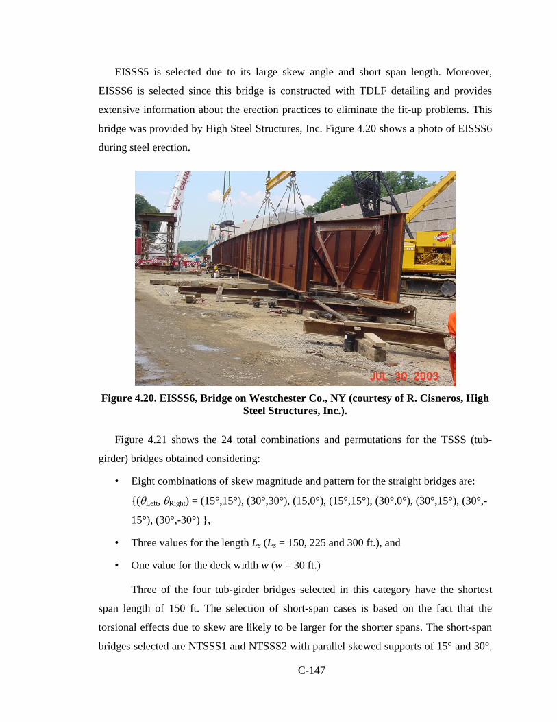
C-147

EISSS5 is selected due to its large skew angle and short span length. Moreover,

EISSS6 is selected since this bridge is constructed with TDLF detailing and provides

extensive information about the erection practices to eliminate the fit-up problems. This

bridge was provided by High Steel Structures, Inc. Figure 4.20 shows a photo of EISSS6

during steel erection.

Figure 4.20. EISSS6, Bridge on Westchester Co., NY (courtesy of R. Cisneros, High

Steel Structures, Inc.).

Figure 4.21 shows the 24 total combinations and permutations for the TSSS (tub-

girder) bridges obtained considering:

• Eight combinations of skew magnitude and pattern for the straight bridges are:

{(θLeft, θRight) = (15°,15°), (30°,30°), (15,0°), (15°,15°), (30°,0°), (30°,15°), (30°,-

15°), (30°,-30°) },

• Three values for the length Ls (Ls = 150, 225 and 300 ft.), and

• One value for the deck width w (w = 30 ft.)

Three of the four tub-girder bridges selected in this category have the shortest

span length of 150 ft. The selection of short-span cases is based on the fact that the

torsional effects due to skew are likely to be larger for the shorter spans. The short-span

bridges selected are NTSSS1 and NTSSS2 with parallel skewed supports of 15° and 30°,

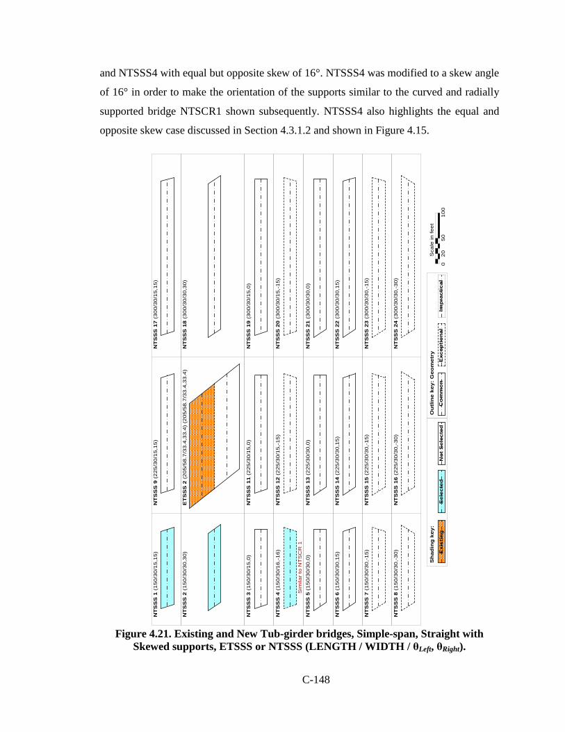
C-148

and NTSSS4 with equal but opposite skew of 16°. NTSSS4 was modified to a skew angle

of 16° in order to make the orientation of the supports similar to the curved and radially

supported bridge NTSCR1 shown subsequently. NTSSS4 also highlights the equal and

opposite skew case discussed in Section 4.3.1.2 and shown in Figure 4.15.

NT

SS

S 1

(1

50

/30

/15

,15

)N

TS

SS

9 (

22

5/3

0/1

5,1

5)

NT

SS

S 1

7 (3

00

/30

/15

,15

)

NT

SS

S 2

(1

50

/30

/30

,30

)E

TS

SS

2 (

20

5/5

8.7

/33

.4,3

3.4

) (2

05

/58

.7/3

3.4

,33

.4)

NT

SS

S 1

8 (3

00

/30

/30

,30

)

NT

SS

S 6

(1

50

/30

/30

,15

)N

TS

SS

14

(22

5/3

0/3

0,1

5)

NT

SS

S 2

2 (3

00

/30

/30

,15

)

NT

SS

S 7

(1

50

/30

/30

,-1

5)

NT

SS

S 1

5 (2

25

/30

/30

,-1

5)

NT

SS

S 2

3 (3

00

/30

/30

,-1

5)

NT

SS

S 4

(1

50

/30

/16

,-1

6)

NT

SS

S 1

2 (2

25

/30

/15

,-1

5)

NT

SS

S 8

(1

50

/30

/30

,-3

0)

NT

SS

S 1

6 (2

25

/30

/30

,-3

0)

NT

SS

S 2

4 (3

00

/30

/30

,-3

0)

NT

SS

S 3

(1

50

/30

/15

,0)

NT

SS

S 1

1 (2

25

/30

/15

,0)

NT

SS

S 1

9 (3

00

/30

/15

,0)

NT

SS

S 5

(1

50

/30

/30

,0)

NT

SS

S 1

3 (2

25

/30

/30

,0)

NT

SS

S 2

1 (3

00

/30

/30

,0)

Sh

adin

g k

ey:

Ou

tlin

e ke

y: G

eom

etry

Exi

stin

gN

ot

Sel

ecte

dC

om

mo

nE

xcep

tio

nal

Imp

ract

ical

Sca

le in

fe

et

02

05

01

00

Sim

ilar

to N

TS

CR

1

NT

SS

S 2

0 (3

00

/30

/15

,-1

5)

Sel

ecte

d

Figure 4.21. Existing and New Tub-girder bridges, Simple-span, Straight with

Skewed supports, ETSSS or NTSSS (LENGTH / WIDTH / θLeft, θRight).

C-149

In addition to the above bridges, the NTSSS10 bridge was selected to study the

influence of an increase in the span length when the skew support angle is kept constant.

The NTSSS10 bridge was replaced by the existing ETSSS2 (Sylvan Bridge). The Sylvan

bridge (Figure 4.22) has a span length of 205 ft. and was constructed in two individual

longitudinal phases with deck widths of 58.7 ft. and parallel skewed supports of 33.4°.

Figure 4.22. ETSSS 2, Sylvan Bridge over Sunset Highway, Multomah Co., OR

(courtesy of Homoz Seradj, Oregon DOT).

4.3.4.3 Continuous-Span Bridges, Straight, with Skewed Supports (ICSS and TCSS)

Figure 4.23 shows four of the six groups of ICSS bridges. The six groups correspond

to the combinations of three span lengths and the two deck widths. Two different widths

30 and 80 ft. were considered for L =150 ft. in Figure 4.23, but only 80 ft. wide bridges

were considered for L = 250 and 350 ft. This is because the effect of skew was expected

to be smaller for the narrower longer-span bridges. Furthermore, for the bridges with L =

250 and 350 ft. and w = 30 ft. are not shown since these combinations and permutations

were found to be exceptional due to their large length-to-width ratios.

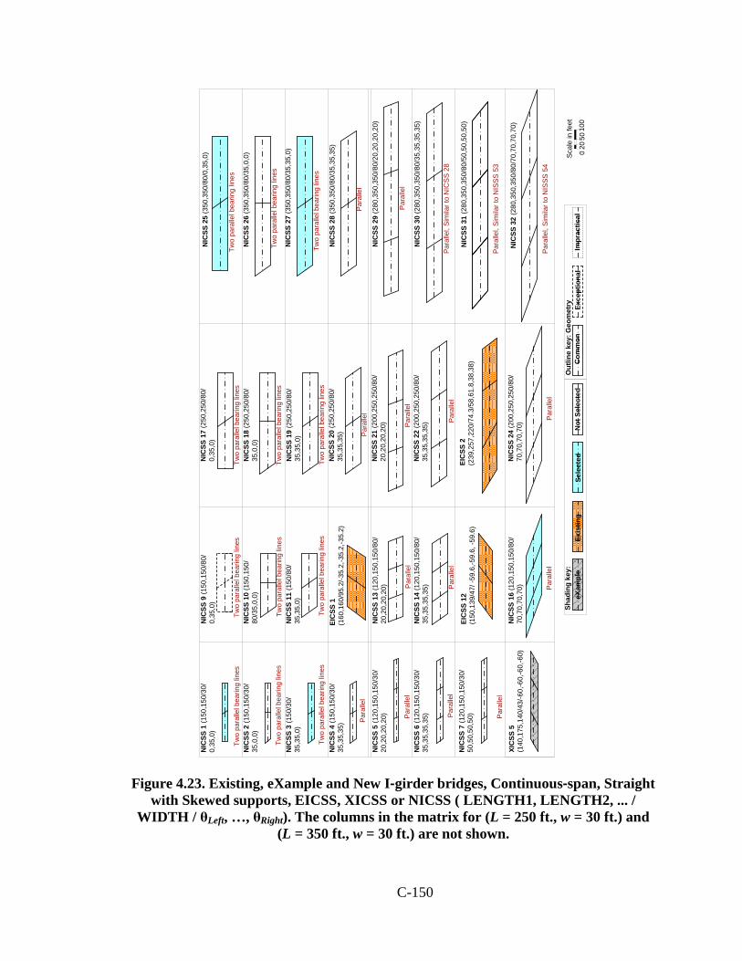
C-150

Para

llel

Two

para

llel b

earin

g lin

esTw

o pa

ralle

l bea

ring

lines

Two

para

llel b

earin

g lin

es

Two

para

llel b

earin

g lin

esTw

o pa

ralle

l bea

ring

lines

Two

para

llel b

earin

g lin

es

Two

para

llel b

earin

g lin

esTw

o pa

ralle

l bea

ring

lines

Two

para

llel b

earin

g lin

es

Para

llel

Para

llel

Para

llel

Para

llel

Para

llel

Para

llel

Para

llel

Para

llel,

Sim

ilar t

o N

ICSS

28

Para

llel

Two

para

llel b

earin

g lin

es

Two

para

llel b

earin

g lin

es

Two

para

llel b

earin

g lin

es

Para

llel

Para

llel

Para

llel

NIC

SS 7

(120

,150

,150

/30/

50,5

0,50

,50)

Scal

e in

feet

020

5010

0

Shad

ing

key:

Out

line

key:

Geo

met

rySe

lect

edEx

istin

geX

ampl

eN

ot S

elec

ted

Com

mon

Exce

ptio

nal

Impr

actic

al

NIC

SS 9

(150

,150

/80/

0,35

,0)

NIC

SS 1

7 (2

50,2

50/8

0/0,

35,0

)N

ICSS

25

(350

,350

/80/

0,35

,0)

NIC

SS 1

0 (1

50,1

50/

80/3

5,0,

0)N

ICSS

18

(250

,250

/80/

35,0

,0)

NIC

SS 2

6 (3

50,3

50/8

0/35

,0,0

)

NIC

SS 2

0 (2

50,2

50/8

0/35

,35,

35)

NIC

SS 2

8 (3

50,3

50/8

0/35

,35,

35)

NIC

SS 1

1 (1

50/8

0/35

,35,

0)N

ICSS

19

(250

,250

/80/

35,3

5,0)

NIC

SS 2

7 (3

50,3

50/8

0/35

,35,

0)

NIC

SS 1

3 (1

20,1

50,1

50/8

0/20

,20,

20,2

0)N

ICSS

21

(200

,250

,250

/80/

20,2

0,20

,20)

NIC

SS 2

9 (2

80,3

50,3

50/8

0/20

,20,

20,2

0)

NIC

SS 2

2 (2

00,2

50,2

50/8

0/35

,35,

35,3

5)N

ICSS

30

(280

,350

,350

/80/

35,3

5,35

,35)

NIC

SS 1

6 (1

20,1

50,1

50/8

0/70

,70,

70,7

0)N

ICSS

32

(280

,350

,350

/80/

70,7

0,70

,70)

NIC

SS 1

(150

,150

/30/

0,35

,0)

NIC

SS 2

(150

,150

/30/

35,0

,0)

NIC

SS 4

(150

,150

/30/

35,3

5,35

)

NIC

SS 3

(150

/30/

35,3

5,0)

NIC

SS 5

(120

,150

,150

/30/

20,2

0,20

,20)

NIC

SS 6

(120

,150

,150

/30/

35,3

5,35

,35)

NIC

SS 3

1 (2

80,3

50,3

50/8

0/50

,50,

50,5

0)

NIC

SS 1

4 (1

20,1

50,1

50/8

0/35

,35,

35,3

5)

NIC

SS 2

4 (2

00,2

50,2

50/8

0/70

,70,

70,7

0)

Para

llel

Para

llel,

Sim

ilar t

o N

ISSS

53

Para

llel,

Sim

ilar t

o N

ISSS

54

EIC

SS 1

(1

60,1

60/9

5.2/

-35.

2,-3

5.2,

-35.

2)

EIC

SS 2

(2

39,2

57,2

20/7

4.3/

58,6

1.8,

38,3

8)

XIC

SS 5

(140

,175

,140

/43/

-60,

-60,

-60,

-60)

EIC

SS 1

2(1

50,1

39/4

7/ -5

9.6,

-59.

6, -5

9.6)

Figure 4.23. Existing, eXample and New I-girder bridges, Continuous-span, Straight with Skewed supports, EICSS, XICSS or NICSS ( LENGTH1, LENGTH2, ... /

WIDTH / θLeft, …, θRight). The columns in the matrix for (L = 250 ft., w = 30 ft.) and (L = 350 ft., w = 30 ft.) are not shown.

C-151

In Figure 4.23, the top four rows of the matrix include four two-span continuous

bridges with unequal skew and one case with parallel skew. Only values of θ = 35o were

considered for these selected cases.

The case with the parallel skew (EICSS1) is a steel overpass on Sunnyside Road

Interchange, (I-15B) over I-15, in Bonneville County, ID. This bridge represents a

successful implementation of total dead load fit detailing, which aims to ensure that the

webs are plumb under the total steel plus concrete dead load. Both field observations and

field data are available for this bridge. Figure 4.24 shows the gap at the sole plate at one

of the bearings of this bridge under the steel dead load. Although daylight is apparent

between the sole plate and the elastomeric bearing pad on one side under the steel dead

load condition, the girders rotated as expected during the deck placement such that full

contact was established with the elastomeric pads. Figure 4.25 shows the lack of fit

between one of the girder connection plates and the bolt holes in a cross-frame during the

steel erection on this bridge. This was expected and intentional due in part to the total

dead load fit of the cross-frames. That is, the holes in the girder connection plates and in

the cross-frame plates had to be aligned. This hole alignment was achieved on the

Sunnyside Road job using drift pins without any other mechanical aid.

Trends in the behavior for other skews were targeted by the ISSS cases in Figure 4.18

and the ICCS cases discussed subsequently (see Figure 4.41). The last four rows of

Figure 4.23 are three-span continuous designs with parallel skew. Two cases with

unequal skew and a narrower deck, NICSS1 and 3, were selected for L = 150 ft. and two

comparable cases but with the wider deck, NICSS25 and 27, were selected for L = 350 ft.

Parallel skews with the extreme skew angles were considered by selecting bridges

XICSS5 and NICSS16, with L = 150 ft. and w = 30 ft. and 80 ft. for the 3-span continu-

ous designs.

The bridge XICSS5 is taken from the NHI Course No.130081A-D (NHI, 2007),

which is an LRFD eXample design developed by Grubb et al. (2007) for the National

Highway Institute. Since detailed design calculations are shown for this structure, it was

selected to serve as an excellent example for the benchmarking.

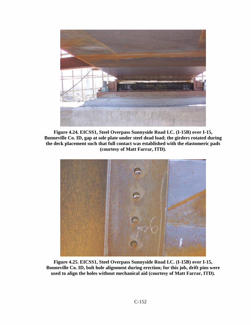
C-152

Figure 4.24. EICSS1, Steel Overpass Sunnyside Road I.C. (I-15B) over I-15,

Bonneville Co. ID, gap at sole plate under steel dead load; the girders rotated during the deck placement such that full contact was established with the elastomeric pads

(courtesy of Matt Farrar, ITD).

Figure 4.25. EICSS1, Steel Overpass Sunnyside Road I.C. (I-15B) over I-15,

Bonneville Co. ID, bolt hole alignment during erection; for this job, drift pins were used to align the holes without mechanical aid (courtesy of Matt Farrar, ITD).

C-153

In addition, several cases involving 3-span continuous designs with parallel skews

were selected due availability of similar Existing bridges in the literature:

• EICSS2 is located at I-235 EB over E. University Ave., Polk County, IA. This

bridge, recommended by Iowa DOT, had difficulty with the installation of cross-

frames during the steel erection. According to Iowa DOT, the fabricator detailed

and fabricated the cross-frames for the final dead load condition, i.e., total dead

load fit. The problem was resolved by requiring the fabricator to supply new

cross-frames that were detailed for steel dead load fit. The bridge has an

interesting combination of a relatively wide deck, and substantial unequal skew of

the bearing lines. Therefore, it represents a potentially useful case where total

dead load fit detailing may be problematic.

• EICSS12 is located at US 82 main lane underpass at 19th stress west bound,

Lubbock County, TX. This bridge is one of several suggested by TxDOT. This

bridge involves a field implementation and evaluation of the use of lean-on cross-

frames to alleviate issues of nuisance stiffness in significantly skewed bridges and

to eliminate cross-frame diagonals within a large portion of the bridge framing.

The design and construction of this bridge are discussed by Helwig et al. (2003).

Field data are reported by Romage (2008). This bridge provided an outstanding

potential opportunity for validation or verification of the refined analysis methods

utilized in the NCHRP research versus available experimental and analytical

results.

Figure 4.26 shows the combinations and permutations for the two and three

continuous-span TCSS (tub-girder) bridges considering:

• Eight combinations of skew magnitude and pattern for the two-span straight

bridges: {(θLeft, θRight) = (0°, 15°,0°), (0°, 0°, 15°), (0°, 15°, 15°), (15°, 15°, 15°),

(0°, 30°, 0°), (0°, 0°, 30°), (0°, 30°, 30°), (30°, 30°, 30°)},

• Two combinations of skew magnitude and pattern for the three-span straight

bridges: {(θLeft, θRight) = (15°, 15°, 15°), (30°, 30°, 30°)},

• Two values for the length Ls (Ls = 150, 250 ft.), Ls = 350 ft. are not shown, and

C-154

NTC

SS 4

(150

,150

/30/

15,1

5,15

)

NTC

SS 1

8 (2

50, 2

50/3

0/30

,30,

30)

NTC

SS 1

4 (2

50,2

50/3

0/15

,15,

15)

NTC

SS 8

(150

,150

/30/

30,3

0,30

)

NTC

SS 1

(150

,150

/30/

0,15

,0)

NTC

SS 1

1 (2

50,2

50/3

0/0,

15,0

)

NTC

SS 5

(150

,150

/30/

0,30

,0)

NTC

SS 1

5 (2

50,2

50/3

0/0,

30,0

)

NTC

SS 2

(150

,150

/30/

0,0,

15)

NTC

SS 6

(150

,150

/30/

0,0,

30)

NTC

SS 1

2 (2

50,2

50/3

0/0,

0,15

)

NTC

SS 1

6 (2

50,2

50/3

0/0,

0,30

)

NTC

SS 9

(120

,150

,150

/30/

15/1

5,15

,15)

NTC

SS 2

0 (2

00,2

50,2

50/3

0/30

/30,

30,3

0)

NTC

SS 1

9 (2

00,2

50,2

50/3

0/15

/15,

15,1

5)

NTC

SS 1

0 (1

20,1

50,1

50/3

0/30

/30,

30,3

0)

NTC

SS 3

(150

,150

/30/

0,15

,15)

NTC

SS 7

(150

,150

/30/

0,30

,30)

NTC

SS 1

3 (2

50,2

50/3

0/0,

15,1

5)

NTC

SS 1

7 (2

50,2

50/3

0/0,

30,3

0)

Shad

ing

key:

Out

line

key:

Geo

met

ry

Sele

cted

Not

Sel

ecte

dC

omm

onEx

cept

iona

lIm

prac

tical

Scal

e in

feet

020

5010

0

Sim

ilar t

o N

TCSS

9

Sim

ilar t

o N

TCSS

10

Figure 4.26. New Tub-girder bridges, Continuous-span, Straight with Skewed supports, NTCSS (LENGTH1, LENGTH2, … / WIDTH / θLeft, …, θRight). The

columns in the matrix for (L = 350 ft., w = 30 ft.) are not shown.

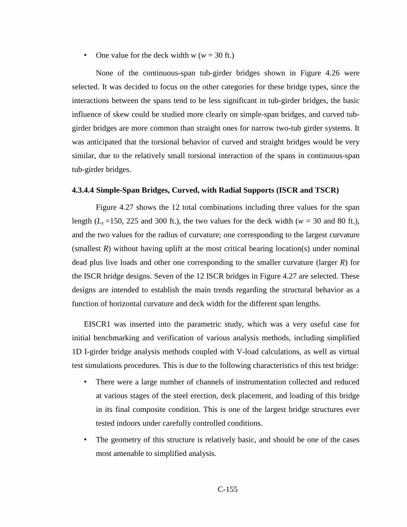
C-155


None of the continuous-span tub-girder bridges shown in Figure 4.26 were

selected. It was decided to focus on the other categories for these bridge types, since the

interactions between the spans tend to be less significant in tub-girder bridges, the basic

influence of skew could be studied more clearly on simple-span bridges, and curved tub-

girder bridges are more common than straight ones for narrow two-tub girder systems. It

was anticipated that the torsional behavior of curved and straight bridges would be very

similar, due to the relatively small torsional interaction of the spans in continuous-span

tub-girder bridges.

4.3.4.4 Simple-Span Bridges, Curved, with Radial Supports (ISCR and TSCR)

Figure 4.27 shows the 12 total combinations including three values for the span

length (Ls =150, 225 and 300 ft.), the two values for the deck width (w = 30 and 80 ft.),

and the two values for the radius of curvature; one corresponding to the largest curvature

(smallest R) without having uplift at the most critical bearing location(s) under nominal

dead plus live loads and other one corresponding to the smaller curvature (larger R) for

the ISCR bridge designs. Seven of the 12 ISCR bridges in Figure 4.27 are selected. These

designs are intended to establish the main trends regarding the structural behavior as a

function of horizontal curvature and deck width for the different span lengths.

EISCR1 was inserted into the parametric study, which was a very useful case for

initial benchmarking and verification of various analysis methods, including simplified

1D I-girder bridge analysis methods coupled with V-load calculations, as well as virtual

test simulations procedures. This is due to the following characteristics of this test bridge:

• There were a large number of channels of instrumentation collected and reduced

at various stages of the steel erection, deck placement, and loading of this bridge

in its final composite condition. This is one of the largest bridge structures ever

tested indoors under carefully controlled conditions.

• The geometry of this structure is relatively basic, and should be one of the cases

most amenable to simplified analysis.

C-156

Shading key: Outline key: GeometrySelectedExisting Not Selected Common Exceptional Impractical

Scale in feet

0 20 50 100

EISCR 1 (90 / 200 / 23.5)

Similar to EICCR 25

NISCR 2 (150/438/30)

NISCR 7 (150/280/80)

NISCR 8 (150/420/80)

NISCR 11 (300/730/80)NISCR 5 (300/1530/30)

NISCR 9 (225/470/80)NISCR 3 (225/930/30)

NISCR 12 (300/1095/80)NISCR 6 (300/2295/30)

NISCR 10 (225/705/80)NISCR 4 (225/1395/30)

IT = 0.71

IT = 0.69

IT = 0.62

IT = 0.58

IT = 0.71

IT = 0.65

IT = 0.59

Figure 4.27. Existing and New I-girder bridges, Simple-span, Curved with Radial

supports, EISCR or NISCR (LENGTH / RADIUS / WIDTH).

• This test bridge was designed at or slightly above a number of maximum limits in

the AASHTO LRFD Specifications. Hence a number of its characteristics are

likely to accentuate the effect of certain analysis and/or design approximations.

Jung (2006) and Jung and White (2008) provide a detailed discussion of the

characteristics and the behavior of this test bridge. These references also provide

substantial prior results from FEA simulation models similar to the types of simulation

models that are employed in the NCHRP research. Figure 4.28 shows a view of the

FHWA test bridge at an intermediate stage of the steel erection, when the first two of the

C-157

three girders in this bridge had been placed on their support bearings and connected

together by cross-frames.

Figure 4.28. EISCR1, FHWA Test Bridge (Jung, 2006, Jung and White, 2008).

Figure 4.29 shows the 6 combinations for the TSCR (tub-girder) bridges obtained

considering:

• Three values for the span length Ls (Ls = 150, 225 and 300 ft.),

• One value for the deck width w (w = 30 ft.), and

• Two values of the curvature radii R for each span length.

NTSCR1 and NTSCR2 (IT = 0.83 and 0.72) were selected to study for the effects

for different curvature at the shorter span length. One bridge, NTSCR5 (IT = 0.87), was

selected to study the effect of larger span length for similar IT.

C-158

Scale in feet

0 20 50 100

Similar to XTCCR8

NTSCR 1 (150/400/30)

NTSCR 2 (150/600/30)

NTSCR 3 (225/820/30)

NTSCR 4 (225/1230/30)

NTSCR 5 (300/1360/30)

NTSCR 6 (300/2040/30)

Shading key: Outline key: Geometry

Selected Not Selected Common Exceptional Impractical

IT = 0.83

IT = 0.72

IT = 0.87

Figure 4.29. New Tub-girder bridges, Simple-span, Curved with Radial supports,

NTSCR (LENGTH / RADIUS / WIDTH).

4.3.4.5 Continuous-Span Bridges, Curved, with Radial Supports (ICCR and TCCR)

Figure 4.30 shows 12 total combinations of Ls (= 150, 250 and 350 ft.), w (= 30

and 80 ft.) and the two conceptual values for the radius of curvature discussed previously

in Section 4.3.1.1, for the ICCR bridges. The first radius of curvature corresponds to the

largest curvature (smallest R) without having uplift at the most critical bearing location(s)

under nominal dead plus live loads and the second corresponds to 1.5 times this R value.

In Figure 4.30, all of the cases with the narrower deck are selected, as shown in the

first column of this parametric study design matrix, except NICCR5. The selection is

mainly driven by the Existing bridge designs. EICCR22a was selected since it has

extensive field observations and measurements, reported by Leon et al. (2011). Figure

4.31 shows a photo of EICCR22a during its steel erection.

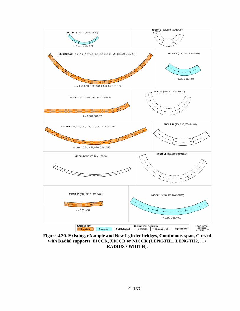
C-159

EICCR 11 (321, 445, 292 / ∞, 511 / 48.2)

Scale in feet

0 20 50 100

Shading key: Outline key: GeometryExisting Selected Not Selected Common Exceptional Impractical

EICCR 4 (222, 260, 210, 162, 256, 190 / 1108, ∞ / 44)

EICCR 15 (210, 271 / 1921 / 48.9)

NICCR 1 (150,150,120/227/30)NICCR 7 (150,150,120/150/80)

NICCR 8 (150,150,120/308/80)

NICCR 9 (250,250,200/250/80)

NICCR 10 (250,250,200/491/80)

NICCR 11 (350,350,280/413/80)

NICCR 12 (350,350,280/909/80)

NICCR 5 (350,350,280/1153/30)

EICCR 22 a (172, 217, 217, 195, 171, 172, 162, 192 / 791,889,746,766 / 43)

IT = 087, 0.87, 0.74

IT = 0.60, 0.63, 0.66, 0.63, 0.60,0.60, 0.59,0.62

IT = 0.50,0.50,0.87

IT = 0.61, 0.64, 0.59, 0.56, 0.64, 0.50

IT = 0.55, 0.58

IT = 0.61, 0.61, 0.58

IT = 0.66, 0.66, 0.61

Figure 4.30. Existing, eXample and New I-girder bridges, Continuous-span, Curved

with Radial supports, EICCR, XICCR or NICCR (LENGTH1, LENGTH2, ... / RADIUS / WIDTH).

C-160

Figure 4.31. EICCR22a, Bridge No. 12 Ramp B over I-40, Robertson Avenue

Project, Davidson Co., TN.

EICCR11, which is the Ford City Bridge, in Ford City, PA, was inserted into the

analytical study since it represents an important model case where due to combinations of

long spans, deep girders with relatively close spacing compared to the girder depths, and

relatively tight curvature, substantial erection challenges had to be addressed in the

erection engineering of the structure. This bridge has been studied thoroughly in prior

work by Chavel and Earls (2006a & b; 2001) as well as by Chang (2006). Hence, it

represented another valuable case that can be used to validate the analysis and design

methods. Figure 4.32 shows an overall photo of the Ford City bridge during its steel

erection. Figure 4.33 emphasizes the overall depth of the girders relative to their

horizontal spacing. Figure 4.34 provides several snapshots during the installation of a key

drop-in segment on this bridge. The circles in these photos are highlighting a come-along

beam that is being used to stabilize the curved girder during lifting. A cable goes to the

lifting beam from each end of the come-along beam.

C-161

Figure 4.32. EICCR11, Ford City Bridge, Ford City, PA (Chavel, 2008).

Figure 4.33. EICCR11, Ford City Bridge, Ford City, PA, girder depth and spacing

(Chavel, 2008).

C-162

Figure 4.34. EICCR11, Ford City Bridge, Ford City, PA, installation of drop-in

segment (Chavel, 2008).

EICCR4 is one of the units of Ramp GG, John F. Kennedy Memorial Highway, I-95

Express Toll Lanes and I-695 Interchange, Baltimore County, MD. High Steel Structures,

Inc. did the fabrication and the steel erection for this bridge. Several members of the

NCHRP 12-79 team visited the job site with the High Steel engineers to observe the

erection of a drop-in segment on the second span from the right hand end of this bridge in

the sketch during August 2007. Figure 4.35 is a photo of the bridge just prior to

installation of this drop-in segment.

EICCR15 is located at SR 6220 A11 over SR 6220 NB and SB, Centre County, PA.

This bridge was studied experimentally and analytically by Shura (2004) and is discussed

by Domalik et al. (2005). Due to its unequal span lengths (ratio of the span lengths of

0.77), this bridge exhibits important torsional interactions between its two spans. The

shorter span actually twists in the direction opposite from the torsional deformation of the

longer span. That is, the downward deflection of girders toward the outside of the curve

C-163

in the longer span corresponds to an upward deflection of the girders toward the inside of

the curve on the shorter span. As a result, this bridge was selected to serve as an

important case for assessment of the sufficiency or limitations of various simplified

analysis methods.

Figure 4.35. EICCR4, Ramp GG John F. Kennedy Memorial Highway, I-95 Express

Toll Lanes and I-695 Interchange, Baltimore Co., MD (courtesy of R. Cisneros, High Steel Structures, Inc.).

In addition, two of the three cases with wider decks and smaller curvature (larger R)

were considered in the second column of the matrix. The wider-deck cases with tighter

curvature in Figure 4.30 were considered to be exceptional designs. The influence of

wide decks with tight curvatures was expected to be captured sufficiently via the

combination of the ISCR and ISCS bridges.

Figure 4.36 is based on the combinations for the TCCR (tub-girder) bridges with

three continuous-spans considering:

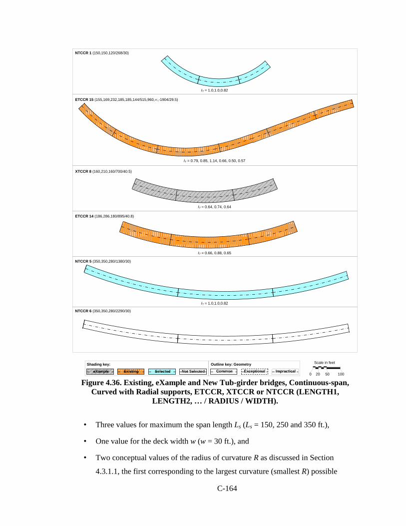
C-164



Scale in feet

0 20 50 100eXample

NTCCR 1 (150,150,120/268/30)

ETCCR 15 (155,169,232,185,185,144/515,960,∞,-1904/29.5)

XTCCR 8 (160,210,160/700/40.5)

ETCCR 14 (186,286,180/895/40.8)

NTCCR 5 (350,350,280/1380/30)

NTCCR 6 (350,350,280/2290/30)

Existing

IT = 1.0,1.0,0.82

IT = 0.79, 0.85, 1.14, 0.66, 0.50, 0.57

IT = 0.64, 0.74, 0.64

IT = 0.66, 0.88, 0.65

IT = 1.0,1.0,0.82

Figure 4.36. Existing, eXample and New Tub-girder bridges, Continuous-span,

Curved with Radial supports, ETCCR, XTCCR or NTCCR (LENGTH1, LENGTH2, … / RADIUS / WIDTH).

• Three values for maximum the span length Ls (Ls = 150, 250 and 350 ft.),

• One value for the deck width w (w = 30 ft.), and

• Two conceptual values of the radius of curvature R as discussed in Section

4.3.1.1, the first corresponding to the largest curvature (smallest R) possible

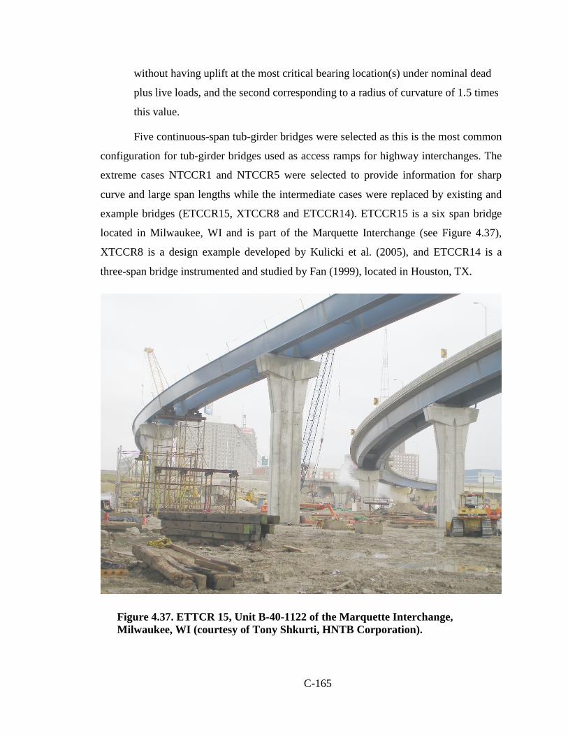
C-165

without having uplift at the most critical bearing location(s) under nominal dead

plus live loads, and the second corresponding to a radius of curvature of 1.5 times

this value.

Five continuous-span tub-girder bridges were selected as this is the most common

configuration for tub-girder bridges used as access ramps for highway interchanges. The

extreme cases NTCCR1 and NTCCR5 were selected to provide information for sharp

curve and large span lengths while the intermediate cases were replaced by existing and

example bridges (ETCCR15, XTCCR8 and ETCCR14). ETCCR15 is a six span bridge

located in Milwaukee, WI and is part of the Marquette Interchange (see Figure 4.37),

XTCCR8 is a design example developed by Kulicki et al. (2005), and ETCCR14 is a

three-span bridge instrumented and studied by Fan (1999), located in Houston, TX.

Figure 4.37. ETTCR 15, Unit B-40-1122 of the Marquette Interchange, Milwaukee, WI (courtesy of Tony Shkurti, HNTB Corporation).

C-166

4.3.4.6 Simple-Span Bridges, Curved, with Skewed Supports (ISCS and TSCS)

Figure 4.38 displays four of the 12 groups of I-girder bridges considering:

• The twelve combinations of skew magnitude.

• The two values for length, Ls = 150 and 300 ft.

• The two values for the deck width w = 30 and 80 ft.

• The four values of radius of curvature R = 438, 280, 420 and 730 ft. which were

selected from ISCR bridges.

Since the effects of skew are generally larger in wider bridges for a given span length,

emphasis was placed on bridges with the wider decks in the design of the ISCS studies.

In addition, none of the bridges with 225 ft. span length are considered in Figure 4.38.

This is because it was expected that the interactions between the effects of the curvature

and skew on I-girder bridges can be captured sufficiently by studying the ISSS, ICSS,

ISCR, ICCR, ISCS and ICCS bridges with Ls = 150 ft.

One case with Ls = 300 ft., the case with the wider deck and tighter curvature, was

included to investigate the interaction effect on a longer-span design where some type of

flange-level lateral bracing system is likely.

In Figure 4.38 one can observe that the bridges in the 2nd and 3rd rows of 1st, 2nd and

3rd columns were selected except NSCS1 and NSCS3 for analytical studies. These

bridges were selected to capture the behavior with respect to the variation in the Ls /w and

Ls /R ratios. NISCS9 was selected to capture the effect of parallel skewed bearings along

with curvature effects.

EISCS3 was inserted into the design matrix. This bridge is SR 8002 Ramp A-1, in

King of Prussia, PA, studied extensively by Chavel and Earls (2003) and Chavel (2008)

in their prior research (see Figure 4.39). Moreover, the third phase of the EISCS4 was

inserted into the study matrix since this phase experienced large differential

displacements with respect to the adjacent units due to its large length-to-width ratio.

C-167

Scale in feet

0 2050 100

Shading key: Outline key: GeometryExisting Selected Not Selected Common Exceptional Impractical

NISCS 3 (150/438/30/-35,0)

NISCS 1 (150/438/30/19.6,0)

NISCS 7 (150/438/30/-35,-35)

NISCS 5 (150/438/30/9.8,-9.8)

NISCS 15 (150/280/80/-35,0)

NISCS 13 (150/280/80/30.7,0)

NISCS 19 (150/280/80/-35,-35)

NISCS 17 (150/280/80/15.3,-15.3)

NISCS 27 (150/420/80/-35,0)

NISCS 31 (150/420/80/-35,-35)

NISCS 25 (150/420/80/35,0)

NISCS 29 (150/420/80/10.2,-10.2)

NISCS 9 (150/438/30/65.2,45.6)

NISCS 21 (150/280/80/53.7,23) NISCS 33 (150/420/80/58.2,37.7)

NISCS 8 (150/438/30/-65.2,-35)

NISCS 20 (150/280/80/-53.7,-35)

NISCS 32 (150/420/80/-58.2,-35)

NISCS 39 (300/730/80/-35,0)

NISCS 41 (300/730/80/11.8,-11.8)

NISCS 45 (300/730/80/62.6,39.1)

NISCS 44 (300/730/80/-62.6,-35)

NISCS 4 (150/438/30/-65.2,0)

NISCS 10 (150/438/30/-35.2,35.2)

NISCS 12 (150/438/30/65.2,-65.2)

NISCS 14 (150/280/80/53.7,0)

NISCS 16 (150/280/80/-53.7,0)

NISCS 22 (150/280/80/-29.7,29.7)

NISCS 24 (150/280/80/53.7,-53.7)

NISCS 26 (150/420/80/58.2,0)

NISCS 28 (150/420/80/-58.2,0)

NISCS 34 (150/420/80/-34.8,34.8)

NISCS 36(150/420/80/58.2,-58.2)

NISCS 37 (300/730/80/35,0)

NISCS 40 (300/730/80/-62.6,0)

NISCS 46 (300/730/80/-33.2,33.2)

NISCS 48 (300/730/80/62.6,-62.6)

NISCS 6 (150/438/30/65.2,-35)

NISCS 18 (150/280/80/53.7,-35) NISCS 30 (150/420/80/58.2,-35)

NISCS 42 (300/730/80/62.6,-35)

NISCS 11 (150/438/30/65.2,65.2)

NISCS 23 (150/280/80/53.7,53.7)

NISCS 35 (150/420/80/58.2,58.2)

NISCS 47 (300/730/80/62.6,62.6)

Parallel

θmin = -70°

Parallel, θmax = 70°

θmax = 70°, both ends

θmin = -70°, θmax = 70°

Perpendicular Perpendicular, Laso/Lasi>2


θmax = 70°

θmin = -70°, Laso/Lasi>2

θmax = 70°, Lasi/Laso>2



Parallel, θmax = 70°

Perpendicular, Laso/Lasi>2

θmin = -70°, θmax = 70°, Lasi/Laso>2 θmin = -70°, θmax = 70°


Parallel, θmax = 70°, Similar to NISCS 38

Perpendicular

θmin = -70°

θmax = 70°

NISCS 38 (300/730/80/62.6,0)

θmax = 70°

Parallel

θmin = -70°

θmax = 70°

Parallel Parallel

θmax = 70°

65.7° between supports


Parallel, Similar to NISCS 13

θmax = 70°, Lasi/Laso>2


Parallel, θmax = 70°,Similar to NISCS 14

θmin = -70°,θmax = 70°, Lasi/Laso>2

86.1° between supports

Parallel, Similar to NISCS 25

EISCS 3 (151/279/35.6/50.8,0)

EISCS 4 (252/2269/27.3/-18.4,-24.7)

Figure 4.38. Existing and New I-girder bridges, Simple-span, Curved with Skewed

supports, EISCS or NISCS (LENGTH / RADIUS / WIDTH / θLeft, θRight). The columns in the matrix for (L = 150 ft., w =30 ft., R = 292 ft.), (L = 225 ft., w =30 ft., R = 930 and 1395 ft.), (L = 225 ft., w =80 ft., R = 470 and 705 ft.), (L = 300 ft., w =30 ft.,

R = 1530 and 2295 ft.) and (L = 300 ft., w =80 ft., R = 1095 ft.) are not shown.

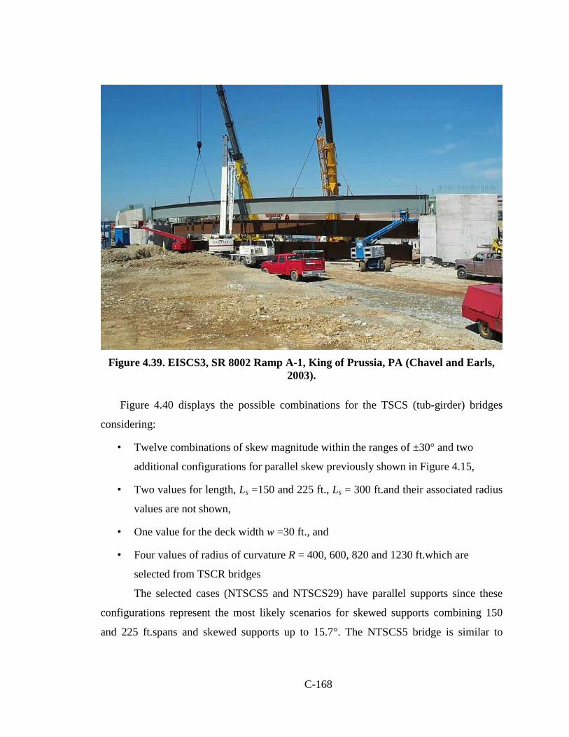
C-168

Figure 4.39. EISCS3, SR 8002 Ramp A-1, King of Prussia, PA (Chavel and Earls,

2003).

Figure 4.40 displays the possible combinations for the TSCS (tub-girder) bridges

considering:

• Twelve combinations of skew magnitude within the ranges of ±30° and two

additional configurations for parallel skew previously shown in Figure 4.15,

• Two values for length, Ls =150 and 225 ft., Ls = 300 ft.and their associated radius

values are not shown,

• One value for the deck width w =30 ft., and

• Four values of radius of curvature R = 400, 600, 820 and 1230 ft.which are

selected from TSCR bridges

The selected cases (NTSCS5 and NTSCS29) have parallel supports since these

configurations represent the most likely scenarios for skewed supports combining 150

and 225 ft.spans and skewed supports up to 15.7°. The NTSCS5 bridge is similar to

C-169

NTSSS4 shown in Figure 4.21, which has an equal and opposite skew angle at its

abutments. The NTSCS29 bridge has skew at only one of its supports.

Scale in feet

0 20 50 100



NTSCS 11 (150/400/30/30,30) NTSCS 39 (225/820/30/30,30)NTSCS 25 (150/600/30/30,30) NTSCS 53 (225/1230/30/30,30)

NTSCS 8 (150/400/30/-30,-15) NTSCS 36 (225/820/30/-30,-15)NTSCS 22 (150/600/30/-30,-15) NTSCS 50 (225/1230/30/-30,-15)

NTSCS 4 (150/400/30/-30,0) NTSCS 32 (225/820/30/-30,0)NTSCS 18 (150/600/30/-30,0) NTSCS 46 (225/1230/30/-30,0)



NTSCS 9 (150/400/30/30,8.5) NTSCS 37 (225/820/30/0.75 /30,14.3)

NTSCS 23 (150/600/30/30,15.7) NTSCS 51 (225/1230/30/30,19.5)

NTSCS 7 (150/400/30/-15,-15) NTSCS 35 (225/820/30/-15,-15)NTSCS 21 (150/600/30/-15,-15) NTSCS 49 (225/1230/30/-15,-15)



NTSCS 2 (150/400/30/21.5,0) NTSCS 30 (225/820/30/30,0)NTSCS 16 (150/600/30/30,0) NTSCS 44 (225/1230/30/30,0)

NTSCS 1 (150/400/30/15,0) NTSCS 29 (225/820/30/15.7,0)NTSCS 15 (150/600/30/14.3,0) NTSCS 43 (225/1230/30/10.5,0)

NTSCS 6 (150/400/30/30,-15) NTSCS 34 (225/820/30/30,-15)NTSCS 20 (150/600/30/30,-15) NTSCS 48 (225/1230/30/30,-15)

NTSCS 5 (150/400/30/10.7,-10.7) NTSCS 33 (225/820/30/7.9,-7.9)NTSCS 19 (150/600/30/7.2,-7.2) NTSCS 47 (225/1230/30/5.2,-5.2)

NTSCS 12 (150/400/30/30,-30) NTSCS 40 (225/820/30/30,-30)NTSCS 26 (150/600/30/30,-30) NTSCS 54 (225/1230/30/30,-30)

Parallel

Parallel

Parallel

Parallel ParallelParallel

Parallel Parallel

Similar to NTCCS 24

Parallel ParallelParallel Parallel

IT = 0.81

IT = 0.84

Figure 4.40. New Tub-girder bridges, Simple-span, Curved with Skewed supports,

NTSCS (LENGTH / RADIUS / WIDTH / θLeft, θRight). The columns in the matrix for (L = 350 ft., w = 30 ft., R = 1390 and 2085 ft.) are not shown.

C-170

4.3.4.7 Continuous-Span Bridges, Curved, with Skewed Supports (ICCS and TCCS)

Figure 4.41 shows six of the 12 possible groups of ICCS bridges. Note that the R

values selected for the ICCR bridges (Figure 4.30) were used also for the subsequent

ICCS designs in Figure 4.41. Rows 1 through 3 of the parametric study design matrix

shown in this figure correspond to different orientations of the bearing lines relative to

the curved geometry, but with the bearing lines parallel (or near parallel in cases where

the skew angle is limited by θ = + 70o at the inside edge of the deck). The bridges in the

fourth row are similar to those in row 1, but with zero skew at the bearing line at the right

hand end of the bridge. Three of the four combinations of deck width and horizontal

curvature for L = 150 ft.are considered in columns 1 through 3 of this matrix. Narrow 250

ft.continuous-spans with the tighter curvature are considered in the fourth column. This

case was included because ramp type structures with roughly 250 ft.span lengths are very

common. The last two columns of Figure 4.41 show 350 ft.two-span continuous bridges

with 80 ft.wide decks and each of the values of horizontal curvature determined

previously. The narrower bridges were not considered for these span lengths, since it was

expected that the influence of skew will be more minor for these bridges. Lastly, all the

150 ft.span bridges in column 1 of the Figure 4.41 test matrix were selected. In addition,

all the 250 and 350 ft.span bridges in columns 4 and 6 were selected except the ones with

perfect symmetry about the center pier (NICCS15 and 23) and NICCS22 since this bridge

is similar to NICCR12. The case with perfect symmetry about the center pier was

believed to be less common for these types of bridge geometry. The two non-exceptional

cases with the wider decks were considered in the third column of this parametric study

design matrix. NICCS11 was not selected since this bridge is similar to NICCR8 in

Figure 4.30.

EICCS 10 was inserted into the design matrix. This is the MN DOT Bridge No.

27998, TH94 between 27th Avenue and Huron Boulevard in Minneapolis, MN. This

bridge has been studied extensively, both experimentally and analytically, by Galambos

et al. (1996). Also, it has been used by Nowak et al. (2006) as part of the calibration of

the AASHTO LRFD Specifications for curved steel bridges. Therefore, this bridge was

C-171

selected to be of particular value in relating the implications of analysis accuracy in the

context of structural reliability calibration and assessment of strengths.

Scal

e in

feet

0 20 5

0 100

Shad

ing

key:

Out

line

key:

Geo

met

ryeX

ampl

eEx

istin

gSe

lect

edN

ot S

elec

ted

Com

mon

Exce

ptio

nal

Impr

actic

alNIC

CS

23 (3

50,3

50/9

09/8

0/0.

65/2

2.1,

0,-

22.1

)N

ICC

S 7

(150

,150

/150

/80/

- 43.

6,0,

43.6

)

Para

llel

Para

llel

Para

llel

Para

llel,

Sim

ilar t

o N

ICC

S 17

Two

para

llel b

earin

g lin

esTw

o pa

ralle

l be

arin

g lin

es, θ

max

= 7

0°

Sam

e as

NIC

CS

5

Two

para

llel

bear

ing

lines

Two

para

llel b

earin

g lin

es

Para

llel,

θmax

= 7

0°

Two

para

llel b

earin

g lin

es

Two

para

llel b

earin

g lin

es

θmin =

-70°

,θm

ax =

70°

Tw

o pa

ralle

l bea

ring

lines

,θm

in =

-70°

, θm

ax =

70°

Para

llel

Para

llel

Two

para

llel b

earin

g lin

es

Para

llel

Two

para

llel b

earin

g lin

es

EIC

CS

10

(145

,150

/286

/33.

4/40

.1,3

4.8,

-10.

4)

EIC

CS

1 (2

04,2

78,2

52,1

85/7

57/4

0.2/

0,0,

32.7

,0,0

)

Two

para

llel b

earin

g lin

es

XIC

CS7

(160

,210

,160

/700

/40.

5/ 0

,-60,

-60,

0)

EIC

CS

27(2

79,2

24,2

36/2

546/

88 /-

53.1

,-59.

4,-6

4.4,

-69.

7)

NIC

CS

2(1

50,1

50/2

27/3

0/38

,0,0

)

NIC

CS

3 (1

50,1

50/2

27/3

0/38

,0,-3

8)

NIC

CS

5 (1

50,1

50/1

50/8

0/43

.6,0

,-43.

6)

NIC

CS

6 (1

50,1

50/1

50/8

0/43

.6,-1

3.8,

0)

NIC

CS

8 (1

50, 1

50/1

50/8

0/43

.6,1

3.8,

-43

.6)

NIC

CS

9 (1

50,1

50/3

08/8

0/56

,28,

0)

NIC

CS

10 (1

50,1

50/3

08/8

0/28

,0,0

)

NIC

CS

11 (1

50,1

50/3

08/8

0/28

,0,-2

8)

NIC

CS

12 (1

50,1

50/

308/

80/0

,28,

0)

NIC

CS

14(2

50,2

50/5

97/3

0/24

.0,0

,0)

NIC

CS

15 (2

50,2

50/5

97/3

0/24

.0,0

,-24.

0)

NIC

CS

13 (2

50,2

50/5

97/3

0/47

.9,2

4.0,

0)N

ICC

S 17

(3

50,3

50/4

13/8

0/58

.1,9

.5,-3

9.0)

NIC

CS

18 (3

50,3

50/4

13/8

0/49

.0,0

,0)

NIC

CS

20

(350

,350

/413

/80/

0,9.

5,-3

9.0)

NIC

CS

19

(350

,350

/413

/80/

49.0

,0,-4

9.0)

NIC

CS

22 (3

50,3

50/9

09/8

0/22

.1,0

,0)

NIC

CS

24 (3

50,3

50/9

09/8

0/0,

22.1

,0)

Figure 4.41. Existing and New I-girder bridges, Continuous-span, Curved with

Skewed supports, EICCS or NICCS (LENGTH1, LENGTH2, ... / RADIUS / WIDTH / θLeft, …, θRight). The columns in the matrix for (L = 150 ft., w =30 ft., R = 438 ft.), (L = 250 ft., w =30 ft., R = 1179 ft.), (L = 250 ft., w =80 ft., R = 250 and 491

ft.), (L = 350 ft., w =30 ft., R = 1153 and 2291 ft.) are not shown.

C-172

EICCS1 was also inserted into the parametric study matrix. This bridge is the I-459 /

US31 Interchange Flyover A in Jefferson County, AL. The construction of this bridge

was observed and thoroughly documented by Osborne (2002). This bridge represents a

successful implementation of total dead load fit detailing on a significantly curved span

with one pier location that is substantially skewed relative to a radial line. Figure 4.42

shows a photo looking along the length of the bridge at the skewed bearing line during

construction. Figure 4.43 shows another snapshot of the steel erection.

Figure 4.42. EICCS1, I-459 / US31 Interchange Flyover A, Jefferson Co. AL

(Osborne, 2002).

Figure 4.44 shows the two-span continuous TCCS (tub-girder) bridges considering:

• Eight combinations of skew magnitude and pattern when only one support is

skewed in the rage of ±30° and two additional configurations when two supports

are skewed to accommodate three parallel support lines,

• Two values for the length Ls (Ls = 150 and 250 ft.), Ls = 350 ft.and their

associated radius values are not shown,

• Two values of the curvature radii R for each span length, and


C-173

Figure 4.43. EICCS1, I-459 / US31 Interchange Flyover A, Jefferson Co. AL

(Osborne, 2002).

In this category several cases fall into the exceptional cases since a 30° skew for

curved bridges distorts the geometry at the support lines causing undesired layouts for a

narrow configuration. Two existing bridges with an intermediate skewed support were

included in this category (ETCCS5a and ETCCS6) and a third case was selected

NTCCS22.

NTCCS22, which has a moderate skew of 20° at one abutment, was selected

because this configuration results in two parallel support lines. ETCCS5a, which is

located at the SR 9A and SR202 interchange in Duval Co. FL, has an intermediate

support that is skewed at 4.8°. These two bridges were targeted to gain insight about the

effect of skew at an intermediate support and at the abutment.

C-174

Sh

adin

g k

ey:

Ou

tlin

e ke

y: G

eom

etry

Exi

stin

gN

ot

Sel

ecte

dC

om

mo

nE

xcep

tio

nal

Imp

ract

ical

Sca

le in

fe

et

02

05

01

00

NT

CC

S 5

(1

50

,15

0/2

68

/30

/30

,0,0

)N

TC

CS

25

(25

0,2

50

/71

3/3

0/3

0,0

,0)

NT

CC

S 1

5 (1

50

,15

0/4

38

/30

/30

,0,0

)N

TC

CS

35

(25

0,2

50

/11

79

/30

/30

,0,0

)

NT

CC

S 6

(1

50

,15

0/2

68

/30

/15

,0,0

)N

TC

CS

26

(25

0,2

50

/71

3/3

0/1

5,0

,0)

NT

CC

S 1

6 (1

50

,15

0/4

38

/30

/15

,0,0

)N

TC

CS

36

(25

0,2

50

/11

79

/30

/15

,0,0

)

NT

CC

S 7

(1

50

,15

0/2

68

/30

/-1

5,0

,0)

NT

CC

S 2

7 (2

50

,25

0/7

13

/30

/-1

5,0

,0)

NT

CC

S 3

7 (2

50

,25

0/1

17

9/3

0/-

15

,0,0

)

NT

CC

S 8

(1

50

,15

0/2

68

/30

/-3

0,0

,0)

NT

CC

S 2

8 (2

50

,25

0/7

13

/30

/-3

0,0

,0)

NT

CC

S 1

8 (1

50

,15

0/4

38

/30

/-3

0,0

,0)

NT

CC

S 3

8 (2

50

,25

0/1

17

9/3

0/-

30

,0,0

)

NT

CC

S 9

(1

50

,15

0/2

68

/30

/0,3

0,0

)N

TC

CS

29

(25

0,2

50

/71

3/3

0/0

,30

,0)

NT

CC

S 1

9 (1

50

,15

0/4

38

/30

/0,3

0,0

)N

TC

CS

39

(25

0,2

50

/11

79

/30

/0,3

0,0

)

NT

CC

S 1

0 (1

50

,15

0/2

68

/30

/0,1

5,0

)N

TC

CS

30

(25

0,2

50

/71

3/3

0/0

,15

,0)

NT

CC

S 4

0 (2

50

,25

0/1

17

9/3

0/0

,15

,0)

NT

CC

S 4

(1

50

,15

0/2

68

/30

/0,3

2.0

,0)

NT

CC

S 2

4 (2

50

,25

0/7

13

/30

/0,2

0.1

,0)

NT

CC

S 1

4 (1

50

,15

0/4

38

/30

/0,1

9.6

,0)

NT

CC

S 3

4 (2

50

,25

0/1

17

9/3

0/0

,12

.2,0

)

NT

CC

S 2

(1

50

,15

0/2

68

/30

/32

.0,0

,0)

NT

CC

S 2

2 (2

50

,25

0/7

13

/30

/20

.1,0

,0)

NT

CC

S 1

2 (1

50

,15

0/4

38

/30

/19

.6,0

,0)

NT

CC

S 3

2 (2

50

,25

0/1

17

9/3

0/1

2.1

,0,0

)

NT

CC

S 3

(1

50

,15

0/2

68

/30

/32

,0,-

32

.0)

NT

CC

S 2

3 (2

50

,25

0/7

13

/30

/20

.1,0

,-2

0.1

)N

TC

CS

13

(15

0,1

50

/43

8/3

0/1

9.6

,0,-

19

.6)

NT

CC

S 3

3 (2

50

,25

0/1

17

9/3

0/1

2.1

,0,-

12

.1)

NT

CC

S 1

(1

50

,15

0/2

68

/30

/64

.1,3

2.0

,0)

NT

CC

S 2

1 (2

50

,25

0/7

13

/30

/40

.2,2

0.1

,0)

NT

CC

S 1

1 (1

50

,15

0/4

38

/30

/39

.2,1

9.6

,0)

NT

CC

S 3

1 (2

50

,25

0/1

17

9/3

0/2

4.3

,12

.1,0

)

Pa

ralle

l

Tw

o p

ara

llel b

ea

rin

g li

ne

s

Tw

o p

ara

llel b

ea

rin

g li

ne

s

Pa

ralle

l

Pa

ralle

l

Tw

o p

ara

llel b

ea

rin

g li

ne

s

Tw

o p

ara

llel b

ea

rin

g li

ne

s

Pa

ralle

l

Pa

ralle

l

Tw

o p

ara

llel b

ea

rin

g li

ne

s

Tw

o p

ara

llel b

ea

rin

g li

ne

s

Pa

ralle

l

Pa

ralle

l

Tw

o p

ara

llel b

ea

rin

g li

ne

s

Tw

o p

ara

llel b

ea

rin

g li

ne

s

Pa

ralle

l

ET

CC

S 6

(1

68

, 1

93

/ 8

01

/ 2

5.3

/ 0

, -3

9.9

, 0

)

(1

82

, 2

20

/ 8

27

/ 2

5.3

/ 0

, -3

8.4

, 0

)

ET

CC

S 5

a (

18

5,1

64

/ 7

65

/ 3

0 /

0,-

4.8

,0)

Sel

ecte

d

Figure 4.44. Existing and New Tub-girder bridges, Continuous-span, Curved with

Skewed supports, ETCCS or NTCCS (LENGTH1, LENGTH2, … / RADIUS / WIDTH / θLeft, …, θRight). The columns in the matrix for (L = 350 ft., w = 30 ft.,

R = 1380 and 2291 ft.) are not shown.

C-175

ETCCS6 is the Magruder Blvd. bridge over I-64 in Hampton, VA. This bridge

was constructed in two phases, with 2 tub-girders each phase, and has a maximum skew

angle of 40° at the interior phase. This bridge does not include any external cross-frames

or diaphragms between the girders at its skewed interior support, and it does not contain

any intermediate external diaphragms between the girders within its spans. Figure 4.45

shows the underside of the completed Magruder Blvd. bridge.

Figure 4.45. ETCCS6, McGruder Blvd. bridge over I-64 in Hampton, VA.

4.3.4.8 Tub-Girder Skew Sensitivity Studies

Skew sensitivity studies were performed for six of the above tub-girder bridges to

assess the impact of skew on the simplified torsional moment estimates. No changes to

the tub-girder bridge original designs were made but minor modifications were made to

accommodate the changes on the framing plan. The bridges and their variations are

NTSSS2 (30°, 15° and 0°), NTSSS4 (16°, 10° and 0°), NTSCS5 (10.7° and 0°),

C-176

NTSCS29 (15.7° and 0°), ETCCS5a (-4.8°, 0°, -10° and 10°) and NTCCS22 (20.1° and

0°). The first angle in the above parentheses corresponds to the original design. The

bridge layouts of the sensitivity studies are shown in Figure 4.46.

NTSSS 2 (150/30/30,30)

NTSSS 4 (150/30/16,-16)

Original Design (16°, -16°)

NTSCS 29 (225/820/30/15.7,0)

NTSCS 5 (150/400/30/10.7,-10.7)

Original Design (10.7°, 10.7°)

Original Design (15.7°, 0°)

NTCCS 22 (250,250/713/30/20.1,0,0)

ETCCS 5 a (185,164 / 765 / 30 / 0,-4.8,0)

Skew (10°, -10°)

Base case (0°, 0°)

Base case (0°, 0°)Skew (15°, 15°)


Original Design (30°, 30°)

Original Design (0°, -4.8°, 0°)

Original Design (20.1°, 0°, 0°)

Base case (0°, 0°, 0°)

Base case (0°,0°, 0°)


Skewed intermediate support (0°, -10°, 0°)

Skewed intermediate support (0°, 10°, 0°)

Figure 4.46. Cases considered in the tub-girder bridge sensitivity studies.

4.3.5 Final Summary of the Parametric Study Bridges

Tables 4.2 and 4.3 provide an overall summary of the number of New, Existing

and eXample bridges developed in the above parametric study design for each of the

major groups of bridges. Eighty-six bridges were selected in total, including 58 I-girder

bridges and 28 tub-girder bridges, or 26 existing bridges and 60 parametric study designs.

C-177

Table 4.2. Overall summary of New, Existing and eXample I-girder bridges.

Description Cases eXample I-girder, Continuous-span, Straight, No skew (Base comparison case) 1

ISSS

(EISSS) Existing, I-girder, Simple-span, Straight, Skewed supports 3 (XISSS) eXample, I-girder, Simple-span, Straight, Skewed supports 0 (NISSS) New, I-girder, Simple-span, Straight, Skewed supports 12

Total: ISSS 15

ICSS

(EICSS) Existing, I-girder, Continuous-span, Straight, Skewed supports 3 (XICSS) eXample, I-girder, Continuous-span, Straight, Skewed supports 1 (NICSS) New, I-girder, Continuous-span, Straight, Skewed supports 5

Total: ICSS 9

ISCR

(EISCR) Existing, I-girder, Simple-span, Curved, Radial supports 1 (XISCR) eXample, I-girder Simple-span, Curved, Radial supports 0 (NISCR) New, I-girder Simple-span, Curved, Radial supports 6

Total: ISCR 7

ICCR

(EICCR) Existing, I-girder, Continuous-span, Curved, Radial supports 4 (XICCR) eXample, I-girder, Continuous-span, Curved Radial supports 0 (NICCR) New, I-girder, Continuous-span, Curved Radial supports 3

Total: ICCR 7

ISCS

(EISCS) Existing, I-girder, Simple-span, Curved, Skewed supports 2 (XISCS) eXample, I-girder, Simple-span, Curved, Skewed supports 0 (NISCS) New, I-girder, Simple-span, Curved, Skewed supports 7

Total: ISCS 9

ICCS

(EICCS) Existing, I-girder, Continuous-span, Curved, Skewed supports 3 (XICCS) eXample, I-girder, Continuous-span, Curved, Skewed supports 1 (NICCS) New, I-girder, Continuous-span, Curved, Skewed supports 6

Total: ICCS 10 Total: Existing I-girder bridges 16 Total: eXample I-girder bridges 3

Total: New I-girder bridges 39 Total: I-girder bridges 58

Appendix E of the NCHRP 12-79 final report provides a concise summary of the most

important considerations for each of the bridges (one-third to one-half page per bridge),

while Appendix K explains the organization of the detailed electronic data for each of the

bridges. Appendix I of the final report provides a more detailed summary of the results

for each of the bridges.

C-178

Table 4.3. Overall summary of New, Existing and eXample tub-girder bridges.

Description Cases eXample Tub-girder, Continuous-span, Straight, No skew (Base comparison case) 1

TSSS

(ETSSS) Existing, Tub-girder, Simple-span, Straight, Skewed supports 1 (XTSSS) eXample, Tub-girder, Simple-span, Straight, Skewed supports 0 (NTSSS) New, Tub-girder, Simple-span, Straight, Skewed supports 3

Total: TSSS 4

TCSS

(ETCSS) Existing, Tub-girder, Continuous-span, Straight, Skewed supports 0 (XTCSS) eXample, Tub-girder, Continuous-span, Straight, Skewed supports 0 (NTCSS) New, Tub-girder, Continuous-span, Straight, Skewed supports 0

Total: TCSS 0

TSCR

(ETSCR) Existing, Tub-girder Simple-span, Curved, Radial supports 0 (XTSCR) eXample, Tub-girder Simple-span, Curved, Radial supports 0 (NTSCR) New, Tub-girder Simple-span, Curved, Radial supports 3

Total: TSCR 3

TCCR

(ETCCR) Existing, Tub-girder, Continuous-span, Curved, Radial supports 2 (XTCCR) eXample, Tub-girder, Continuous-span, Curved, Radial supports 1 (NTCCR) New, Tub-girder, Continuous-span, Curved Radial supports 2

Total: TCCR 5

TSCS

(ETSCS) Existing, Tub-girder, Simple-span, Curved, Skewed supports 0 (XTSCS) eXample, Tub-girder, Simple-span, Curved, Skewed supports 0 (NTSCS) New, Tub-girder, Simple-span, Curved, Skewed supports 2

Total: TSCS 2

TCCS

(ETCCS) Existing, Tub-girder, Continuous-span, Curved, Skewed supports 2 (XTCCS) eXample, Tub-girder, Continuous-span, Curved, Skewed supports 0 (NTCCS) New, Tub-girder, Continuous-span, Curved, Skewed supports 1

Total: TCCS 3 Total: Existing Tub-girder bridges 5 Total: eXample Tub-girder bridges 2

Total: New Tub-girder bridges 11 Total: Additional skew sensitivity studies 10

Total: Tub-girder bridges 28

C-180

5. Assessment of Conventional Simplified Methods of Analysis

NCHRP 12-79 has conducted a wide range of studies on the bridges introduced in

Chapter 4 to determine the ability of the approximate 1D and 2D methods of analysis to capture

the behavior predicted by refined 3D FEA models. The line-girder (1D) analyses of straight I-

and tub-girder bridges, as well as curved tub-girder bridges, were performed using the

STLBRIDGE package (Bridgesoft, Inc., 2010). The line-girder analyses of curved I-girder

bridges were based in the V-load method using the program VANCK (NSBA, 1996). The line-

girder analyses of curved tub-girder bridges were modified using a spreadsheet implementation

of the M/R Method (Tung and Fountain, 1970). In addition, the line-girder analysis results for

skewed tub-girder bridges were modified using the developments described in Sections 2.1.5 and

2.7.1.2. The simplified 2D-grid analyses were conducted using the LARSA 4D (LARSA, 2010)

and MDX (MDX Software, 2011) software systems.

A quantitative assessment of the analysis accuracy was obtained by identifying error

measures that compare the simplified approximate solutions to the 3D second-order elastic FEA

benchmarks. The approach to quantify the error is as follows. First, an error function is defined

as the absolute value of the difference between the FEA representation and the approximate

analysis response, as shown in Figure 5.1. The errors are calculated at the locations along the

length of the girders where the responses are sampled in the approximate method. Next, the error

function is used to calculate the normalized mean error, µe. This index provides an overall

measure of the performance of the approximate models and is calculated as:

𝜇𝑒 = 1

𝑁∙𝑅𝐹𝐸𝐴,𝑚𝑎𝑥∑ 𝑒𝑖𝑁𝑖=1 (5.1)

where N is the total number of sampling points along the girder length used in the simplified

analysis, RFEA,max is the absolute value of the maximum response obtained from the FEA

benchmark, and ei is the absolute value of the error relative to the 3D FEA benchmark solution at

point i. In this equation, the mean error is normalized with respect to the maximum value of the

response obtained from the FEA to avoid a comparison of “small numbers to small numbers.”

For example, the vertical displacements near the supports in a simple-span bridge are relatively

small. The percent error in the response prediction relative to the physical displacement may be

C-181

large at these locations, but the deflections are small compared to the deflections expected near

mid-span. Hence, in Eq. (5.1), the errors are weighted with respect to the maximum value of the

response. In addition, by dividing the error by RFEA,max, the influence of the load magnitude is

removed from the analyses. Given this practice, the mean errors can be compared for different

bridges.

Figure 5.1. Schematic representation of the error function.

5.1 Assessment of I-Girder Bridges

Table 5.1 shows the percent normalized mean errors in the major-axis bending stresses

and vertical displacements obtained for the 58 I-girder bridges studied in the NCHRP 12-79

research. These bridges are divided into six different groups based on their geometry. The first

group corresponds to the curved radially-supported bridges (labeled as “C”) with connectivity

indices IC > 1. As discussed in Section 3.1.3, the connectivity index provides an indication of

when the inaccurate representation of the girder torsional stiffness in conventional 2D-grid

models tends to have a significant impact on the overall error. The second group includes curved

and radial bridges with IC < 1. The straight and skewed structures (labeled as “S”) are subdivided

based on the skew index IS, which differentiates the bridges where skew has a minor influence on

the structural behavior from those where the collateral effects from the skew are more important

(see Section 3.1.2). The groups correspond to IS < 0.30, 0.30 < IS < 0.65, and IS > 0.65. The sixth

group contains the curved and skewed bridges studied in the project (labeled as “C&S”). It is

important to note that the skew and curvature indices, IS and IC should not be used in

combination to estimate the accuracy of the approximate models in a curved and skewed bridge.

C-182

No clear trends in the normalized mean errors were identified as a combined function of IS and IC

with the exception that, as the skew or the horizontal curvature approaches zero, then the error

characteristics should approach the values shown for the “C” and the “S” categories respectively.

Table 5.1 compares the results of the first-order (geometrically linear) 3D FEA, 2D-grid,

and 1D analysis results to the predictions obtained from elastic second-order 3D FEA. In the

table, fb is the major-axis bending stress and Δz is the vertical displacement. A mean error value

is calculated for each response on each girder of the bridges. The values reported in Table 5.1 are

the largest mean errors determined by inspecting the values obtained for each girder in a given

bridge.

Upon inspection of the results in Table 5.1, the following important trends can be

observed:

Second-Order Amplification

The results obtained from the first-order 3D FEA show that the response amplifications

due to second-order effects are negligible in most of the bridges. With the exception of bridges

NISCR5 and EISCS4, the differences between the linear and nonlinear FEA results are less than

10 %. For bridges NISCR5 and EISCS4, the analyses show that these long-and-narrow structures

experience significant global second order amplification. Section 2.9 discusses this behavior in

the context of bridge EISCS4. It should be noted that unless noted otherwise, the benchmark

second-order stresses in Table 5.1 are evaluated at 1.5 times the nominal dead load, correspond-

ing to the AASHTO LRFD Strength IV load combination. However, the benchmark second-

order displacements are evaluated at the nominal (unfactored) dead load level.

It is recommended that the loss of accuracy due to large global second-order amplifica-

tion should be addressed separately from the other factors affecting accuracy. The estimated

global second-order amplification, AFG (Eq. 2.101), is relatively large for the above two bridges.

As noted in Section 2.9, if the AASHTO constructability checks do not pass due to a large AFG,

this should be taken as an indication that a second-order 3D FEA may need to be conducted, or

the design should be changed to avoid the large second-order effects. Therefore, these bridges

are excluded from the subsequent error syntheses.

C-183

Table 5.1. I-girder bridge percent normalized mean errors compared to 3D second-order elastic FEA for major-axis bending stresses (fb) and vertical displacements (∆z).

f b Δz f b Δz f b Δz f b Δz

μe μe μe μe μe μe μe μe

EICCR22a 0 0.98 0.66 1.11 0 0 6 3 4 2 10 6NICCR12 0 0.69 0.66 1.18 1 1 8 7 8 4 9 8EICCR11 0 0.67 0.87 1.17 9 4 11 7 9 3 12 16EICCR4 0 0.68 0.64 1.09 1 1 4 3 6 3 7 5NISCR5a 0 0.58 0.71 1.02 20 9 18 1 15 4 14 19EICCR15 0 0.35 0.58 1.05 3 1 5 3 6 2 12 11EISCR1 0 18.8 0.71 1.09 1 1 8 157 10 147 11 20NISCR7 0 6.70 0.62 1.30 1 1 22 90 17 117 15 13NISCR2 0 4.89 0.69 1.06 3 2 6 38 5 32 6 15NISCR8 0 4.46 0.58 1.19 1 0 11 91 12 97 13 29NICCR1 0 4.13 0.87 1.11 0 0 11 96 7 5 8 10NICCR8 0 3.04 0.61 1.63 0 0 9 57 9 53 7 5NISCR10 0 1.93 0.59 1.11 1 1 12 40 10 37 17 17NISCR11 0 1.08 0.65 1.11 5 2 13 44 6 14 13 16

a NISCR5 is excluded from the error synthesis since this bridge has large second-order amplification. The stresses and displacementsfor this bridge are reported at 1.5 and 1.0 of the TDL respectively.

C (I C > 1)

1D

C (I C < 1)

GroupBridge Name

3D-FEA Linear 2D-Grid - P1 2D-Grid - P2I S I C I T I L

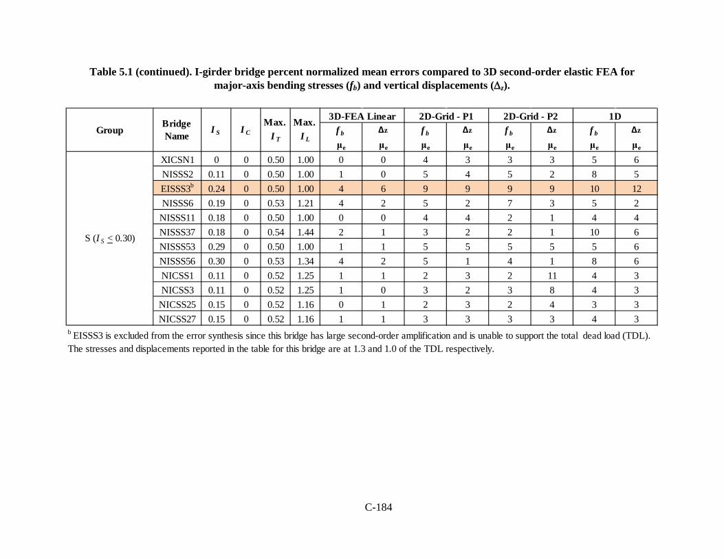
C-184

Table 5.1 (continued). I-girder bridge percent normalized mean errors compared to 3D second-order elastic FEA for major-axis bending stresses (fb) and vertical displacements (∆z).



XICSN1 0 0 0.50 1.00 0 0 4 3 3 3 5 6NISSS2 0.11 0 0.50 1.00 1 0 5 4 5 2 8 5EISSS3b 0.24 0 0.50 1.00 4 6 9 9 9 9 10 12NISSS6 0.19 0 0.53 1.21 4 2 5 2 7 3 5 2

NISSS11 0.18 0 0.50 1.00 0 0 4 4 2 1 4 4NISSS37 0.18 0 0.54 1.44 2 1 3 2 2 1 10 6NISSS53 0.29 0 0.50 1.00 1 1 5 5 5 5 5 6NISSS56 0.30 0 0.53 1.34 4 2 5 1 4 1 8 6NICSS1 0.11 0 0.52 1.25 1 1 2 3 2 11 4 3NICSS3 0.11 0 0.52 1.25 1 0 3 2 3 8 4 3

NICSS25 0.15 0 0.52 1.16 0 1 2 3 2 4 3 3NICSS27 0.15 0 0.52 1.16 1 1 3 3 3 3 4 3

S (I S < 0.30)

GroupBridge Name

3D-FEA Linear 2D-Grid - P1 2D-Grid - P2 1DI S I C

Max. I T

Max. I L

b EISSS3 is excluded from the error synthesis since this bridge has large second-order amplification and is unable to support the total dead load (TDL). The stresses and displacements reported in the table for this bridge are at 1.3 and 1.0 of the TDL respectively.

C-185

Table 5.1 (continued). I-girder bridge percent normalized mean errors compared to 3D second-order elastic FEA for major-axis bending stresses (fb) and vertical displacements (∆z).



NISSS4 0.44 0 0.50 1.00 3 3 9 6 7 6 10 7EISSS5 0.54 0 0.50 1.00 2 2 7 6 4 6 9 8EISSS6 0.43 0 0.50 1.00 3 0 9 5 7 2 6 6

NISSS36 0.40 0 0.55 1.49 3 1 9 2 7 2 8 3XICSS5c 0.53 0 0.50 1.00 1 1 NA NA 16 12 NA NAEICSS1c 0.42 0 0.50 1.00 0 0 NA NA 11 12 NA NAXICSS5 0.53 0 0.50 1.00 1 1 12 8 6 7 16 12EICSS1 0.42 0 0.50 1.00 0 0 4 4 4 6 8 3EICSS2 0.50 0 0.55 1.35 1 0 6 6 6 6 9 8

NISSS13 0.60 0 0.50 1.00 1 1 6 5 5 6 5 5NISSS16 0.59 0 0.58 1.83 2 2 9 6 8 6 9 7EICSS12 0.58 0 0.50 1.00 1 0 7 5 4 3 7 7NISSS14 1.36 0 0.50 1.00 4 0 27 26 26 27 28 27NICSS16 1.69 0 0.50 1.00 1 0 15 12 15 16 15 13NISSS54 0.68 0 0.50 1.00 4 2 17 16 16 13 16 13

1DBridge Name

3D-FEA Linear 2D-Grid - P1 2D-Grid - P2I S I C

Max. I T

Max. I L

S (0.30 0.65)

Group

C-186

Table 5.1 (continued). I-girder bridge percent normalized mean errors compared to 3D second-order elastic FEA for major-axis bending stresses (fb) and vertical displacements (∆z)



EISCS3 0.25 2.99 0.68 0.86 1 1 7 25 5 5 19 38NISCS3 0.11 3.44 0.71 1.18 4 2 10 2 5 1 29 23NISCS9 0.35 3.11 0.63 0.88 2 1 10 36 10 5 24 23NISCS14 0.67 4.46 0.55 0.65 0 0 9 76 7 3 10 15NISCS15 0.36 4.46 0.67 1.88 1 1 19 74 14 12 11 16NISCS37 0.35 1.03 0.35 0.62 1 1 9 42 23 36 37 40NISCS38 0.48 0.94 0.59 0.68 1 0 4 39 4 5 15 18NISCS39 0.17 1.21 0.68 1.32 7 3 13 53 10 2 10 17EISCS4d 0.04 0.55 0.64 1.00 53 52 41 48 43 48 43 50EICCS10 0.16 2.19 0.73 1.07 0 0 10 25 10 19 14 12NICCS2 0.13 3.67 0.87 1.24 0 0 7 36 4 3 9 10NICCS3 0.13 3.30 0.81 0.98 1 0 17 62 5 4 11 13XICCS7 0.36 1.33 0.65 1.51 0 0 12 21 9 9 15 6NICCS9 0.73 3.04 0.58 0.77 0 0 13 73 5 7 8 21NICCS13 0.11 1.05 0.85 0.98 2 1 7 21 3 2 10 13NICCS14 0.04 1.12 0.88 1.04 2 1 6 21 4 3 11 11EICCS1 0.08 0.99 0.80 1.25 1 1 10 20 29 5 30 14EICCS27 0.92 0.17 0.47 0.90 1 0 15 10 17 7 18 11NICCS24 0.09 0.46 0.68 1.18 1 1 6 19 3 1 7 6

2D-Grid - P2 1D

C&S

GroupBridge Name

3D-FEA Linear 2D-Grid - P1I S I C I T I L

d EISCR4 is excluded from the error synthesis since this bridge has large second-order amplification and is unable to support the total dead load (TDL). The stresses and displacements reported in the table for this bridge are at 82 % of the TDL.

C-187

It is recommended that the factor AFG (Eq. 2.101) should be calculated and used in

performing the AASHTO constructability checks for two and three-girder units (or intermediate

stages of the steel erection), as well as for relatively narrow units or intermediate stages with

Ls/wg ratios greater than about five. In addition, in I-girder bridges involving lean-on bracing

systems, the lean-on effects from all the girders being stabilized must be considered. The reader

is referred to Helwig et al. (2005) and Hermann et al. (2005) for presentation of simplified

procedures for checking girder system stability including lean-on effects.

Although the analysis results considered are based on the final constructed geometry of

the bridge for NISCR5, and the final constructed geometry of the bridge unit that experienced

excessive displacements for EISCS4, these results are representative of results that can be

expected for other intermediate stages of the steel erection where the partially completed struc-

ture is composed of only a few girders and/or is relatively narrow compared to the span length.

In addition to global second-order amplification due to stability effects, the potential local

second-order amplification of the flange lateral bending should be checked between the cross-

frame locations in bridge I-girders. Equation 6.10.1.6-4, from AASHTO LRFD Article 6.10.1.6,

serves generally as an accurate to conservative estimate of this local second-order amplification.

In particular, large values of the AF estimated by this equation on fascia girders may indicate a

condition where the flange lateral bending due to overhang eccentric bracket loads and/or

horizontal curvature may lead to excessive torsional rotations that can cause local dips in the

deck elevations between cross-frames. These rotations can be exacerbated by web distortional

deformations in cases where the height of the overhang brackets is significantly less than the

girder web depths. Therefore, local web distortional deformations on fascia girders always

should be checked.

Lastly, the benchmark 3D-FEA model of the “S (IS < 0.30)” bridge EISSS3 is unable to

support the factored total dead load (1.5 x TDL) due to large second-order amplification

associated with the flexibility of the V-type cross-frames without top chords utilized in this

structure. Therefore, EISSS3 is excluded from further consideration in the synthesis of the errors

below. V-type cross-frames without top chords often do not have sufficient stiffness to brace the

I-girders prior to the deck becoming composite. Their effectiveness may often depend on

incidental stiffnesses developed by the formwork or other construction devices serving as top

C-188

chord elements. These incidental stiffnesses can be highly variable and difficult to gage or to

control, and thus the use of V-type cross-frames can result in significant difficulties in the ability

to predict the physical constructed geometry in the field. Therefore, as discussed subsequently in

Chapter 9, V-type cross-frames without top chords should be used with extreme caution.

2D-Grid Solutions

Several observations can be made regarding the 2D-grid solutions from Table 5.1:

• The 2D-grid solutions from Programs P1 and P2 are very similar for the major-axis

bending stresses in all the cases of Table 5.1, with the exception of only three of the

“C&S” bridges, NISCS37, NICCS3, and EICCS1. Program P1 gives significantly better

fb results for NISCS37 and EICCS1, whereas P2 gives much better fb results for NICCS3.

There is no clear reason why the solutions differed significantly for just these three

bridges.

• For all the “C” bridges and for all the “S” bridges, the vertical displacement solutions are

very similar from both 2D-grid programs with the exception of bridges NICCR1 and

NISCR11, where program P2 gives much better results. Similar to the above cases, there

is no clear reason for the larger error exhibited by P1 for just these two bridges.

• For the “S” bridges with IS < 0.30 and 0.30 < IS < 0.65, all of the conventional 2D-grid

solutions for the major-axis bending stresses and vertical displacements are reasonably

good (a more quantitative assessment of the errors as a function of the bridge type is

presented in the next section). However, for the “S” bridges with IS > 0.65, the

conventional 2D-grid solutions give relatively poor predictions for both the major-axis

bending stresses and the displacements. The reason for this behavior is discussed in detail

subsequently in Chapter 6. Basically, due to the poor (highly flexible) girder torsion

model, the conventional 2D-grid solutions are unable to capture the transverse load paths

that develop in skewed bridges with large IS values.

• For the “C” bridges with IC > 1, both the 2D-grid programs P1 and P2 give poor

displacement solutions in the majority of the cases. The only cases of this group where

the results are reasonably accurate are the P2 solutions for bridges NICCR1 and

NISCR11. A key reason for this behavior is explained below.

C-189

• For the “C&S” bridges, the displacement results are reasonably accurate for the 2D-grid

program P2, with the exception of bridges NISCS37 and NICCS10 (after excluding

EISCS4 due to large AFG). However, the 2D-grid program P1 exhibits very large

displacement errors for the majority of the “C&S” bridges. NISCS3 and EICCS27 are the

only bridges that have reasonably accurate displacement predictions from P1. A key

reason for this behavior, as well as for the above poor displacement results for the “C”

bridges with IC > 1, is explained below.

The key reason for the poor displacement results in the last two of the above observations

is the use of multiple elements between the cross-frame locations in modeling the curved girders

in these structures. As noted at the beginning of this chapter, the models in program P1 were

created using four elements between each of the cross-frames for all of the bridges, and the

program P2 models were created with a “high-resolution mesh” for all of the bridges, which

typically means that P2 also uses four elements between each cross-frame member. However, P2

was also set up to include the effect of the composite slab via the Plate-Eccentric Beam approach

in subsequent solutions. The P2 Plate-Eccentric Beam solution is effectively just a 2D-grid

solution prior to the slab being made composite. Unfortunately, program P2 is unable to create a

high-resolution mesh in its Plate-Eccentric Beam solution when a bridge has skew, and hence P2

defaults back to a “low-resolution mesh” in these situations. With a low-resolution mesh in P2,

only one element is utilized between each of the cross-frame members.

Interestingly, contrary to what one might expect, the use of a single element between the

cross-frame locations results in more accurate solutions with the conventional 2D-grid

procedures. The reason for this behavior can be explained in basic terms by considering an

isolated conventional 2D-grid model of an I-section member, subjected to uniform moment

along a circular arc between two cross-frame locations, i.e., equal and opposite end moments

(see Figure 5.2). The vector direction of the moments, by the right-hand rule, is indicated by the

double arrows in the figure. In the common “high-resolution” representation of this curved

member, the arc is modeled with four straight elements, with each of the nodes located along the

arc. Major-axis bending moments perpendicular to the chord between the member ends resolve

into both a major-axis bending and a torsional component within the individual elements. If one

considers the equilibrium at one of the intermediate nodes, major-axis bending in one element is

C-190

generally resolved into both major-axis bending and torsion in the next element. However,

unfortunately, in the conventional methods, the torsional model substantially underestimates the

true stiffness of the I-girder, since only the St. Venant term (GJ/L) is considered. The torsional

stiffness coming from the restraint of warping, related to the cross-section rigidity term ECw, is

neglected. As such, the twisting deformations are grossly over-estimated.

M Mθ1

θ2

M cos θ1

M cos θ1

M cos θ2

M cos θ2

M sin θ1 M sin θ1 M sin θ2M sin θ2

Figure 5.2. Behavior for a chorded representation of a curved I-girder using four straight

elements.

Furthermore, because of the curved geometry (represented in a chorded fashion by the

four elements in Figure 5.2), the small torsional stiffness reduces the overall stiffness of the

approximate model in resisting vertical deflection. The twisting of one element causes not only a

torsional rotation in the next element, but because of the change in orientation of the elements in

the chorded representation of the arc, it causes major-axis bending rotation and corresponding

vertical deflections in the next element. Furthermore, the overall major-axis bending rotational

stiffness that this member provides to the rest of the bridge, about an axis perpendicular to its

chord and at its ends, is reduced by the above effects. This results in an increase in the vertical

deflections at other locations in the bridge.

Interestingly, if a curved I-girder is represented by only one straight element between its

cross-frame locations, the cross-frames are able to resist the components of the moments that

cause twisting of the girder. As a result, the overall model of the bridge structure responds in a

much stiffer fashion. This same behavior is obtained if multiple elements are used between the

cross-frames with the overall geometry represented as a straight chord between the cross-frames.

C-191

(This helps explain why the vertical deflections in straight skewed I-girders are still represented

reasonably well with a high resolution mesh).

Modeling of the girders as straight segments between the cross-frames tends to improve

the results in the conventional 2D-grid analysis of curved bridges, since in effect, this approach

completely neglects the influence of the horizontal curvature between the cross-frames (with the

exception of separate calculations to estimate girder flange lateral bending stresses). Studies

conducted with “C&S” bridges to address this peculiarity demonstrate that the responses

obtained from the P1 models, when the discretization is reduced to one element between every

set of cross-frames, are essentially the same as with the P2 models.

Completely neglecting the horizontal curvature effects between the cross-frames of

course cannot generally produce an accurate model either. Therefore, using a coarse grid of

elements with only one straight element between each cross-frame is not generally recommended

as a proper way to obtain accurate predictions. It should be noted that the “C&S” bridges

NISCS37 and EICCS10 have relatively poor displacement predictions in spite of the fact that the

P2 solutions were based on a single element between each of the cross-frames. Nevertheless, in

many bridges, the girder arcs between the cross-frames are small enough such that a single

element between the cross-frames should be sufficient to accurately represent the overall curved

geometry of the structure (assuming that a more accurate girder torsional stiffness than the

conventional GJ/L is employed, as discussed in Chapter 6). The flange lateral bending stresses

between the cross-frames can still be estimated using “component stress” equations such as Eqs.

(2.13) through (2.17), or by more accurate means as discussed subsequently in Chapter 6.

Chapter 6 discusses modeling practices that can be implemented to improve the

predictions obtained from 2D-grid analyses. The practices discussed in Chapter 6 are based on

the principles of structural mechanics, and do not rely on the discretization level used in the

model. The large errors associated with the more refined discretization are due to the dramatic

under-representation of the girder torsional stiffness in the conventional 2D-grid models, along

with the coupling between twist rotations and vertical displacements in curved members.

C-192

1D Line-Girder Solutions

The 1D line-girder results in Table 5.1 exhibit the following characteristics:

• The solutions are reasonably good for all the “C” bridges with IC < 1. However, for the

“C” bridges with IC > 1, the errors are somewhat larger for several of the bridges,

particularly for the displacements. It should be emphasized that the connectivity index,

IC, relates primarily to the influence of the poor girder torsion model on the overall results

in conventional 2D-grid solutions. However, some correlation of the errors with IC is

evident also for the line-girder analysis solutions.

• For the “S” bridges, the 1D line-girder solutions are comparable in accuracy to the

conventional 2D-grid solutions in all cases. The accuracy is reasonably good using both

the 1D and the conventional 2D grid procedures for the IS < 0.30 and the 0.30 < IS < 0.65

bridges. However, both of these types of solutions show relatively large errors for the

major-axis bending stresses and the vertical displacements for the bridges with IS > 0.65.

Similar to the conventional 2D-grid solutions, 1D line-girder analysis is unable to capture

any information about the transverse load paths in the structure. These load paths tend to

be a significant characteristic of the overall bridge response in bridges with large IS

values. Of course, engineers would not generally expect to capture the transverse load

paths from a 1D line-girder analysis. However, they may expect that these load paths are

captured by a 2D-grid solution.

• For the “C&S” bridges, the errors relative to the 3D FEA benchmarks from the 1D-line

girder analyses are highly variable. There are no clear trends in the data, other than the

fact that the large errors are obviously due to the combination of skew with horizontal

curvature. The V-load method does not have any mechanisms for including the influence

of skew within its estimates, and therefore, one must expect significant errors with

increasing values of skew with this approach. One can observe that the 1D analysis

accuracy tends to be better for some of the bridges that have small IS values. However,

this is not generally the case since, in a curved bridge, the orientation of the skew

(positive or negative) can have a substantial effect on the resulting bridge geometry.

C-193

Staged Deck Placement

For the continuous-span bridges XICSS5 and EICSS1, Table 5.1 shows data both for

analyses where staged deck placement was not considered (generated by building the analysis

models and simply “turning the gravity loads on”) and for analyses where staged deck placement

was considered in the 3D FEA and the conventional 2D-grid solutions. The solutions where the

staged deck placement was considered are highlighted by the shaded rows for XICSS5 and

EICSS1 in Table 5.1. Program P2 was utilized to conduct the 2D-grid solutions for these bridges.

In fact, the Plate Eccentric Beam modeling capabilities of this program were employed to

represent the participation of the composite concrete deck. The deck concrete from previous

stages was assumed to become fully effective in both the 3D FEA and the Plate Eccentric Beam

solutions. Other assumptions are possible regarding the early-age stiffness of the concrete deck;

however, the above assumptions are sufficient to evaluate the accuracy of the Plate Eccentric

Beam solutions versus the 3D FEA benchmarks. In regions of the bridges where the concrete

deck is not fully effective, the Plate Eccentric Beam solution effectively defaults to a conven-

tional 2D-grid solution.

The major-axis bending stress and vertical displacement errors for the above two bridges

are reasonable, but are slightly larger for the analyses considering the staged deck placement.

The scope and number of these studies is not sufficient to draw broad conclusions regarding the

accuracy of the Plate-Eccentric Beam models for general staged deck placement analysis. As

noted at the end of Section 2.10, the primary focus of the NCHRP 12-79 research was on the

overall accuracy of the 1D line-girder and 2D-grid results independent of the participation of the

concrete deck.

C-194

5.1.1 Synthesis of Errors in Major-Axis Bending Stresses and Vertical Displacements for I-Girder Bridges

Table 5.2 shows the number of I-girder bridges within specific ranges of the normalized

mean errors for the major-axis bending stresses and the vertical displacements from Table 5.1.

Both of the 2D-grid programs P1 and P2 are considered, as well as the 1D analysis results. The

selected error ranges are assigned letter grades based on the following criteria:

A: µe < 6 %

B: 6 % < µe < 12 %

C: 12 % < µe < 20 %

D: 20 % < µe < 30 %

F: µe > 30 %

This grading scheme is somewhat arbitrary and was set based on the experience of the NCHRP

12-79 project team. The recommended use of this grading scheme is addressed subsequently.

Depending on the type of response and the consequences of the error, different ranges of error

can be acceptable for different calculations on different jobs. In any case, it is believed that most

engineers would agree that analysis results that do not deviate more than 6 % from a highly

refined benchmark solution are indeed highly accurate. In addition, analysis results where the

errors are larger than 30 % relative to a rigorous benchmark solution might be considered as

highly unreliable.

All of the linear 3D FEA results in the non-shaded rows of Table 5.1 fall within the A

range for the bridges considered with a two minor exceptions, fb for EICCR11 and fb for

NISCS39 which have errors or 9 and 7 % respectively. The differences between the 3D FEA

linear and second-order analysis results in Table 5.1 are due solely to second-order effects.

Bridges EICCR11 and NISCS39 are two of the most extreme geometries considered in the

NCHRP 12-79 project. EICCR11 is the Ford City Bridge, which is a continuous-span four girder

bridge with a 329 ft.curved span, an adjacent 417 ft.straight span, and a 48.3 ft.total deck width.

Therefore, it is not surprising that this bridge would have significant second-order effects. These

effects are detectable using Eq. (2.101) (see Section 2.9). NISCS39 is a wide 300 ft.simple-span

curved bridge with a skew that increases the length of the girder on the outside of the curve.

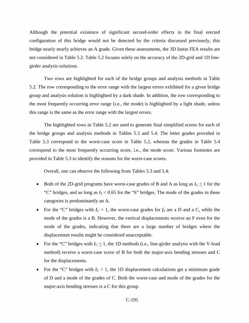
C-195

Although the potential existence of significant second-order effects in the final erected

configuration of this bridge would not be detected by the criteria discussed previously, this

bridge nearly nearly achieves an A grade. Given these assessments, the 3D linear FEA results are

not considered in Table 5.2. Table 5.2 focuses solely on the accuracy of the 2D-grid and 1D line-

girder analysis solutions.

Two rows are highlighted for each of the bridge groups and analysis methods in Table

5.2. The row corresponding to the error range with the largest errors exhibited for a given bridge

group and analysis solution is highlighted by a dark shade. In addition, the row corresponding to

the most frequently occurring error range (i.e., the mode) is highlighted by a light shade, unless

this range is the same as the error range with the largest errors.

The highlighted rows in Table 5.2 are used to generate final simplified scores for each of

the bridge groups and analysis methods in Tables 5.3 and 5.4. The letter grades provided in

Table 5.3 correspond to the worst-case score in Table 5.2, whereas the grades in Table 5.4

correspond to the most frequently occurring score, i.e., the mode score. Various footnotes are

provided in Table 5.3 to identify the reasons for the worst-case scores.

Overall, one can observe the following from Tables 5.3 and 5.4:

• Both of the 2D-grid programs have worst-case grades of B and A as long as IC < 1 for the

“C” bridges, and as long as IS < 0.65 for the “S” bridges. The mode of the grades in these

categories is predominantly an A.

• For the “C” bridges with IC > 1, the worst-case grades for fb are a D and a C, while the

mode of the grades is a B. However, the vertical displacements receive an F even for the

mode of the grades, indicating that there are a large number of bridges where the

displacement results might be considered unacceptable.

• For the “C” bridges with IC < 1, the 1D methods (i.e., line-girder analysis with the V-load

method) receive a worst-case score of B for both the major-axis bending stresses and C

for the displacements.

• For the “C” bridges with IC > 1, the 1D displacement calculations get a minimum grade

of D and a mode of the grades of C. Both the worst-case and mode of the grades for the

major-axis bending stresses is a C for this group.

C-196

Table 5.2. Number of I-girder bridges within specified error ranges for major-axis bending stress and vertical displacement for each of the types of bridges considered.

2D-P1 2D-P2 1D 2D-P1 2D-P2 1DA: < 6% 3 3 0 3 5 2B: 7-12% 2 2 5 2 0 2

C: 13-20% 0 0 0 0 0 1D: 21-30% 0 0 0 0 0 0F: >30% 0 0 0 0 0 0A: < 6% 1 2 1 0 1 1B: 7-12% 5 5 3 0 0 1

C: 13-20% 1 1 4 0 1 5D: 21-30% 1 0 0 0 0 1F: >30% 0 0 0 8 6 0A: < 6% 11 9 8 11 10 11B: 7-12% 0 2 3 0 1 0

C: 13-20% 0 0 0 0 0 0D: 21-30% 0 0 0 0 0 0F: >30% 0 0 0 0 0 0A: < 6% 3 6 2 9 9 4B: 7-12% 7 4 7 1 1 6

C: 13-20% 0 0 1 0 0 0D: 21-30% 0 0 0 0 0 0F: >30% 0 0 0 0 0 0A: < 6% 0 0 0 0 0 0B: 7-12% 0 0 0 1 0 0

C: 13-20% 2 2 2 1 2 2D: 21-30% 1 1 1 1 1 1F: >30% 0 0 0 0 0 0A: < 6% 3 9 0 1 12 2B: 7-12% 11 5 9 1 4 4

C: 13-20% 4 2 5 2 1 7D: 21-30% 0 2 3 5 0 3F: >30% 0 0 1 9 1 2

S (0.30 0.65) 3

C&S (I C > 0.5 & I S > 0.1)

18

C (I C > 1) 8

C (I C < 1) 5

S (I S < 0.30) 11

Major-Axis Bending Stress Vertical DisplacementNumber of Bridges within Error Range

Type of BridgeNumber

of Bridges

Error Range

C-197

Table 5.3. Worst-case I-girder bridge scores for major-axis bending stress and vertical displacement.

2D-P1 2D-P2 1D 2D-P1 2D-P2 1DC (I C < 1) B B B B A Ce

C (I C > 1) Da Ca C F F Df

S (I S < 0.30) A Bb B A Bg AS (0.30 0.65) D D D D D DC&S (I C > 0.5 & I S > 0.1) C D Fd F Fj F

i One bridge with unequal skew, NICSS1, has a mean error of 11 %.j One bridge, NISCS37, has a mean error of 36 %. This is believed to be due to lack of ability of the poor torsional stiffness model in conventional 2D-grid solutions to capture substantial torsional interactions between the girders.

b One bridge with unequal skew, NISSS6, has a mean error of 7 %.

d One bridge, NISCS37, has a mean error of 37 %. The V-load method removes load from the girder on the inside of the curve in this bridge, but the inside girder is the longest because of the skew. The V-load method is not able to capture the corresponding larger bending within the inside girder. e One bridge, EICCR11, has a mean error of 16 %. This larger error is due to torsional interactions between the spans in this continuous-span bridge, which are not captured accurately by the V-Load Method.f One bridge, NISCR8, has a mean error of 29 %. The V-Load Method does not accurately capture the major-axis bending stresses in the interior girders (e.g., Girders 4 and 5) of this wide 9-girder bridgeg One bridge, NICSS3, has a mean error of 8 %, due to over-prediction of the displacements in the first span (having parallel skew) and under-prediction of the displacements in the second span (having unequal skew).

c One bridge with parallel 60o skew, XICSS5, has a mean error of 16 % due to transverse load path (nuisance stiffness) effects.

h One bridge with parallel 60o skew, XICSS5, has a mean error of 8 % due to transverse load path (nuisance stiffness) effects.

a One bridge, NISCR7, has a mean error of 22 % and 17 % for Programs P1 and P2 repectively. This is believed to be due to the combined poor girder torsion model and inaccurate cross-frame stiffness model along with the large width of this bridge. Program P1 has somewhat larger errors than Program P2 because the curved girders were subdivided into multiple elements along each unbraced length in the Program P1 solution.

Type of BridgeWorst Case Scores

Major-Axis Bending Stress Vertical Displacement

C-198

Table 5.4. Mode of I-girder bridge scores for major-axis bending stress and vertical displacement.

• For the “S” bridges with IS > 0.65, both the major-axis bending stresses and the vertical

displacements have a worst-case score of D and a mode of the grades of C in all the

methods.

• For the “C&S” bridges, the major-axis bending stresses received worst-case grades of C

and D with programs P1 and P2 respectively. Furthermore, the 1D analysis major-axis

bending stresses scored a worst-case grade of F due to one bridge exhibiting very poor

results, while most of the bridges scored in the B range. The displacements generally

were very poor for program P1 (due to the discretization of the girder unbraced lengths

into multiple elements), whereas they were usually quite good for program P2, due to the

defaulting of the element discretization to a low-resolution mesh, although one bridge

still fell within the F range with program P2).

It is useful to understand the qualifier indicated on the “C&S” bridges, i.e., “(IC > 0.5 & IS >

0.1)” in Tables 5.3 and 5.4. If a bridge has an IC < 0.5 and an IS > 0.1, it can be considered as a

straight-skewed bridge for the purposes of assessing the expected analysis accuracy. Further-

more, if a bridge has an IC > 0.5 with an IS < 0.1, it can be considered as a curved radially-

supported bridge for these purposes.

2D-P1 2D-P2 1D 2D-P1 2D-P2 1DC (I C < 1) A A B A A BC (I C > 1) B B C F F C

S (I S < 0.30) A A A A A AS (0.30 0.65) C C C C C CC&S (I C > 0.5 & I S > 0.1) B A Ca F A C

a Modified from B to C considering the grade for the C (I C > 1) and S (I S > 0.65) bridges

Type of BridgeMode of Scores

Major-Axis Bending Stress Vertical Displacement

C-199

5.1.2 Generalized I-Girder Bridge Analysis Scores

Table 5.5 provides a synthesis of the analysis scores for the various I-girder bridge

responses from traditional 2D-grid and 1D-line girder methods at large. This table addresses the

accuracy of the calculations for major-axis bending stresses, vertical displacements, cross-frame

forces, flange lateral bending stresses, and girder layovers at the bearings.

Key observations that can be drawn from Table 5.5 are discussed below:

Major-Axis Bending Stresses and Vertical Displacements

For the first two responses in Table 5.5, the major-axis bending stresses and the vertical

displacements, the worst-case and mode letter grades are taken as the lower of the scores for

programs P1 and P2 in Tables 5.3 and 5.4.

Cross-Frame Forces

The accuracy for the third through fifth responses in Table 5.5 can be estimated based on

the grades from the first two responses when considering the “C” bridges. The results for the

third response in these bridge types, the cross-frame forces, are roughly one letter grade less in

accuracy compared to the major-axis bending stresses when evaluated by the traditional 2D-grid

methods. This reduced accuracy is due to the substantial under-representation of the girder

torsional stiffnesses and the crude representation of the cross-frame stiffnesses by prismatic

beam elements in these methods. However, for curved girder bridges the cross-frame forces are

comparable in accuracy to the major-axis bending stresses for the 1D-line girder method (i.e.,

line girder analysis with the V-load method adjustments).

For the straight-skewed bridges with minor skew, i.e., the “S (IS < 0.30)” bridges, the

gravity load cross-frame forces tend to be relatively small; therefore, the corresponding analysis

errors are not of any consequence. However, for straight bridges with larger skew indices, the

major flaws of the 2D-grid methods associated with the poor girder torsion model and the poor

cross-frame models essentially render the cross-frame force estimates as useless. In addition, the

1D-line girder analysis models do not provide any information about the cross-frame forces due

to the skew effects. Therefore, both the traditional 2D-grid and the 1D-line girder analysis

methods get an F for these cases.

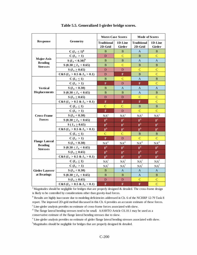
C-200

Table 5.5. Generalized I-girder bridge scores.

Traditional 2D-Grid

1D-Line Girder

Traditional 2D-Grid

1D-Line Girder

C (I C < 1)g B B A BC (I C > 1) D C B C

S (I S < 0.30)h B B A AS (0.30 0.65) D D C CC&S (I C > 0.5 & I S > 0.1) D F B C

C (I C < 1) B C A BC (I C > 1) F D F C

S (I S < 0.30) B A A AS (0.30 0.65) D D C CC&S (I C > 0.5 & I S > 0.1) F F F C

C (I C < 1) C C B BC (I C > 1) F D C C

S (I S < 0.30) NAa NAa NAa NAa

S (0.30 0.65) Fb Fc Fb Fc

C&S (I C > 0.5 & I S > 0.1) Fb Fc Fb Fc

C (I C < 1) C C B BC (I C > 1) F D C C

S (I S < 0.30) NAd NAd NAd NAd

S (0.30 0.65) Fb Fe Fb Fe

C&S (I C > 0.5 & I S > 0.1) Fb Fe Fb Fe

C (I C < 1) NAf NAf NAf NAf

C (I C > 1) NAf NAf NAf NAf

S (I S < 0.30) B A A AS (0.30 0.65) D D C CC&S (I C > 0.5 & I S > 0.1) F F F C

Response GeometryWorst-Case Scores Mode of Scores

Major-Axis Bending Stresses

Vertical Displacements

Cross-Frame Forces

Flange Lateral Bending Stresses

Girder Layover at Bearings

a Magnitudes should be negligible for bridges that are properly designed & detailed. The cross-frame design is likely to be controlled by considerations other than gravity-load forces.b Results are highly inaccurate due to modeling deficiencies addressed in Ch. 6 of the NCHRP 12-79 Task 8 report. The improved 2D-grid method discussed in this Ch. 6 provides an accurate estimate of these forces. c Line-girder analysis provides no estimate of cross-frame forces associated with skew.d The flange lateral bending stresses tend to be small. AASHTO Article C6.10.1 may be used as a conservative estimate of the flange lateral bending stresses due to skew.e Line-girder analysis provides no estimate of girder flange lateral bending stresses associated with skew. f Magnitudes should be negligible for bridges that are properly designed & detailed.

C-201

Table 5.5 (continued). Generalized I-girder bridge scores.

g 15,000( 1)C

cf

IR n m

=+

is the “connectivity index” (see Section 3.1.3 and

Eq. (3.2)), where R is the radius of curvature of the bridge centerline in units of ft., ncf is the number of intermediate cross-frames within the span, and m is a constant equal to 1 for simple-span bridges and 2 for continuous-span bridges.

h tangS

s

wI

Lθ

= is the “skew index” (see Section 3.1.2 and Eq. (3.1)), where

wg is the width of the bridge measured between the centerline of the

fascia girders, θ is the skew angle (equal to zero for zero skew), and Ls is the span length.

Flange Lateral Bending Stresses

For the fourth response in Table 5.5, the flange lateral bending stresses, the accuracies

from the conventional 2D-grid and the 1D-line girder analysis methods for the “C” bridges, are

roughly the same grade as the major-axis bending stresses. This can be understood by

recognizing that the flange lateral bending stresses are generally calculated from Eqs. (2.13)

through (2.16) in these methods (see Sections 2.1.3.1 and 2.1.3.2). Therefore, the estimate of the

maximum flange lateral bending stress from horizontal curvature within the different unbraced

lengths, from Eq. (2.15) or (2.16), is proportional to the estimate of the major-axis bending

stress. Given that the “proportionality factors” multiplying fb in Eq. (2.16) provide a reasonable

(albeit coarse) estimate of the horizontal curvature effects within each of the unbraced lengths,

the accuracy of the flange lateral bending stresses is roughly as good as the accuracy of the

major-axis bending stresses in the “C” bridges.

Unfortunately, for the same reasons as described above for the cross-frame forces, the

estimates of the flange lateral bending stresses in the “S” and “C&S” bridges are unusable when

IS > 0.30. The flange lateral bending stress accuracy for the “C&S” bridges with IS < 0.10 may be

taken roughly as the grade corresponding to its IC value from the “C” bridges.

C-202

Girder Layover at Bearings

As discussed in Section 2.1.4, the girder layovers at skewed bearing lines are closely

related to the girder major-axis bending rotations at the bearings, which are in turn closely tied to

the vertical displacements within the spans. Therefore, the grades for the 2D-grid and the 1D-line

girder estimates of these layovers, the fifth set of responses in Table 5.5, may be taken directly

from the scores for the vertical displacements. Of course, the layover at non-skewed bearing

lines is essentially zero. Therefore, these estimates are Not Applicable (NA) for the “C” bridges.

5.1.3 Assessment Examples for I-girder bridges

Curved I-Girder Bridge: Figure 5.3 shows the plan view of EICCS1, a basic simple-span

bridge with radial supports. It is desired to determine the ability of the approximate analysis

methods to capture the behavior of this structure prior to the slab becoming composite, according

to the scores shown in Table 5.5.

Las = 90 ft./ R = 200 ft./ w = 23.5 ft

Figure 5.3. EICCS1 - Curved and radial simple span I-girder bridge.

This bridge is a relatively simple structure that satisfies the assumptions of the V-load

method derivation. For this bridge, the connectivity index is

IC = 15,000/[(3+1)∙200∙1] = 18.8 > 1.0

According to Table 5.5, the mode grades for the 1D line-girder and 2D-grid models are:

CF3

CF8

C-203

Response Analysis Method 2D-Grid 1D Line-Girder

fb B C Vertical deflections F C Cross-frame forces C C

f C C Girder layovers at bearings NA NA

The mode grades may be considered as the more appropriate characterization of the accuracy of

this bridge because this bridge is “very regular” in its geometry. The worst-case score is likely

the more appropriate one to use when designing a bridge with complicating features such as a

poor span balance, or “less regular” geometry characteristics.

Figures 5.4 through 5.6 show the major-axis bending responses on the outside and inside

fascia girders of the structure. The vertical displacements in Figure 5.4 are shown at the total

noncomposite dead load level (TDL), while fb in Figures 5.5 and 5.6 is shown at 1.5 times TDL

(corresponding to the AASHTO Strengh IV load combination). As shown in Figure 5.4, the

vertical displacements are severely over-predicted by the 2D-grid model. The solution obtained

from a 1D line-girder model is a better representation of the benchmark. By comparing Figures

5.5 and 5.6, it is observed that the approximate methods properly capture fb in the outside girder;

while in the inside girder, the differences are more noticeable. Since the scores are determined

with respect to the girder with the largest errors, which in this case is the inside fascia girder, the

score for fb is B and C for the 2D and 1D methods, respectively.

Figure 5.7 shows the results obtained for the flange lateral bending stresses. In addition,

Table 5.6 shows the cross-frame forces calculated from the 2D-grid and the 3D FEA solutions.

As in the case of the major-axis bending responses, the scores are a good representation of the

predictions obtained with the approximate models. This example shows that the scores are in

agreement with the predictions obtained from the approximate analyses.

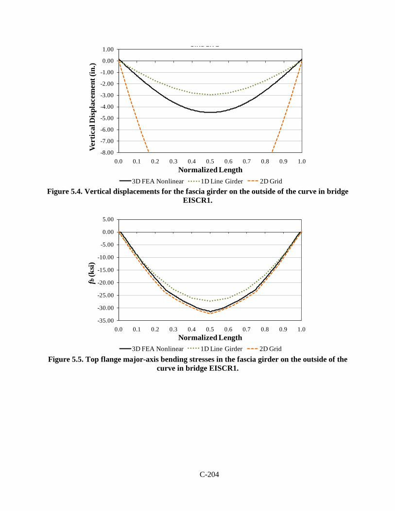
C-204

Figure 5.4. Vertical displacements for the fascia girder on the outside of the curve in bridge

EISCR1.

Figure 5.5. Top flange major-axis bending stresses in the fascia girder on the outside of the

curve in bridge EISCR1.

-8.00

-7.00

-6.00

-5.00

-4.00

-3.00

-2.00

-1.00

0.00

1.00

0.0 0.1 0.2 0.3 0.4 0.5 0.6 0.7 0.8 0.9 1.0

Vert

ical

Dis

plac

emen

t (in

.)

Normalized Length

GIRDER 1

3D FEA Nonlinear 1D Line Girder 2D Grid

-35.00

-30.00

-25.00

-20.00

-15.00

-10.00

-5.00

0.00

5.00

0.0 0.1 0.2 0.3 0.4 0.5 0.6 0.7 0.8 0.9 1.0

fb(k

si)

Normalized Length


C-205

Figure 5.6. Top flange major-axis bending stresses in the fascia girder on the inside of the

curve in bridge EISCR1.

Figure 5.7. Flange lateral bending stresses in the outside fascia girder of bridge EISCR1.

-12.00

-10.00

-8.00

-6.00

-4.00

-2.00

0.00

2.00

0.0 0.1 0.2 0.3 0.4 0.5 0.6 0.7 0.8 0.9 1.0

fb(k

si)

Normalized Length


-30.0

-20.0

-10.0

0.0

10.0

20.0

30.0

40.0

0.0 0.1 0.2 0.3 0.4 0.5 0.6 0.7 0.8 0.9 1.0

f(k

si)

Normalized Length

3D FEA Nonlinear 1D Line Girder-Max2D Grid-Max 3D FEA-Max

C-206

Table 5.6. Cross-frame forces predicted with the 2D-grid and the 3D FEA

Member CF 3 CF8

2D-Grid 3D FEA 2D-Grid 3D

FEA TC 26.6 19.1 24.6 54.5

BC1 -43.1 -46.8 -52.3 -96.6 BC2 -10.1 8.25 3.2 -11.81 D1 23.3 32.7 39.2 49.9 D2 -23.3 -32.3 -39.2 50.2

Skewed I-Girder Bridge: The straight I-girder bridge shown in Figure 5.8, NICSS16, is a

severely skewed structure. It is desired to estimate the accuracy of the predictions obtained from

a line-girder and a 2D-grid analysis for this bridge, according to the scores shown in Table 5.5.

L1 = 120 ft., L2 = 150 ft., L3 = 150 ft./ w = 74 ft./ θ1 = 70 o, θ2 = 70 o, θ3 = 70 o, θ4 = 70 o

Figure 5.8. NICSS 16 - Straight and skewed continuous I-girder bridge.

The skew indices for each span in this structure are 1.69, 1.36, and 1.36, respectively.

These indices are above the 0.65 limit. Hence, it is expected that the skew effects have a

significant contribution to the system response. The following are the mode scores for a bridge

with these characteristics:

Response Analysis Method 2D-Grid 1D Line-Girder

fb C C Vertical deflections C C Cross-frame forces F F

f F F Girder layovers at bearings C C

C-207

As discussed in the previous example, the mode scores may be considered to be the more

appropriate ones here, since the bridge is reasonably “regular,” i.e., no severe span imbalance, no

significant differences in skew angle of the bearing lines, and no significant variations in the

framing of the cross-frames.

Figures 5.9 and 5.10 show the predictions obtained for the girder vertical displacements

and stresses in the structure. For simplicity of the discussions, these responses correspond to no-

load fit detailing of the cross-frames. As shown in Figure 5.9, both analysis methods overpredict

the displacements and stresses in Spans 1 and 3, and slightly underpredict the displacements in

Span 2. Similarly, the major-axis bending stresses shown in Figure 5.10, fb, follow the same

trend. In general, it may be considered that the accuracy of the predictions is reasonable.

Conversely, the responses associated with the flow of transverse forces in the system are

not captured by the approximate methods. As shown in the stress plot, the local f levels are as

high as 43 ksi in Span 3. The cross-frame forces associated with the high f levels are shown in

Figure 5.11. To simplify the observations, they are shown in terms of the cross-frame shear and

bending moments rather than in individual chord and diagonal forces. The figure includes the

responses obtained from the 3D FEA, a traditional grid analysis, and a grid analysis conducted

with the practices recommended in Chapter 6. As shown in the figure, the forces obtained from

the traditional grid model are essentially zero. This is due to the limited representation of the

cross-frames and the girder torsional stiffness in the traditional method. The plots illustrate that,

in this bridge, the physical cross-frame forces are large However, the traditional grid analysis is

not able to capture these forces; hence, it is assigned a grade of F.

C-208

Figure 5.9. Vertical displacement of girder G5 in bridge NICSS16.

Figure 5.10. Top flange stresses in girder G5 of bridge NICSS16.

-5.0

-4.0

-3.0

-2.0

-1.0

0.0

1.0

0.0 0.1 0.2 0.3 0.4 0.5 0.6 0.7 0.8 0.9 1.0

Vert

ical

Dis

plac

emen

t (in

.)

Normalized Length

3D FEA 1D Line Girder 2D Grid Traditional

-50.0

-40.0

-30.0

-20.0

-10.0

0.0

10.0

20.0

30.0

40.0

50.0

0.0 0.1 0.2 0.3 0.4 0.5 0.6 0.7 0.8 0.9 1.0

fb

f

(ksi)

Normalized Length3D FEA-fb 3D FEA-fl 1D Line Girder 2D Grid Traditional

C-209

Figure 5.11. Cross-frame forces in Bay 1 (G1-G2) of NICSS16.

-20.0-15.0-10.0-5.00.05.0

10.015.020.025.030.0

1 2 3 4 5 6 7 8 9 10 11 12 13 14 15 16 17 18 19 20 21

Shea

r For

ce, V

i(k

ips)

Cross-Frame Number

2D Traditional 2D Recommended 3D FEA

i j

-250.0-200.0-150.0-100.0

-50.00.0

50.0100.0150.0200.0

1 2 3 4 5 6 7 8 9 10 11 12 13 14 15 16 17 18 19 20 21

Mom

ent M

i(ki

p-ft

)

Cross-Frame Number


i j

-100.0

-50.0

0.0

50.0

100.0

150.0

200.0

250.0

300.0

1 2 3 4 5 6 7 8 9 10 11 12 13 14 15 16 17 18 19 20 21

Mom

ent M

j(k

ipft

)

Cross-Frame Number


i j

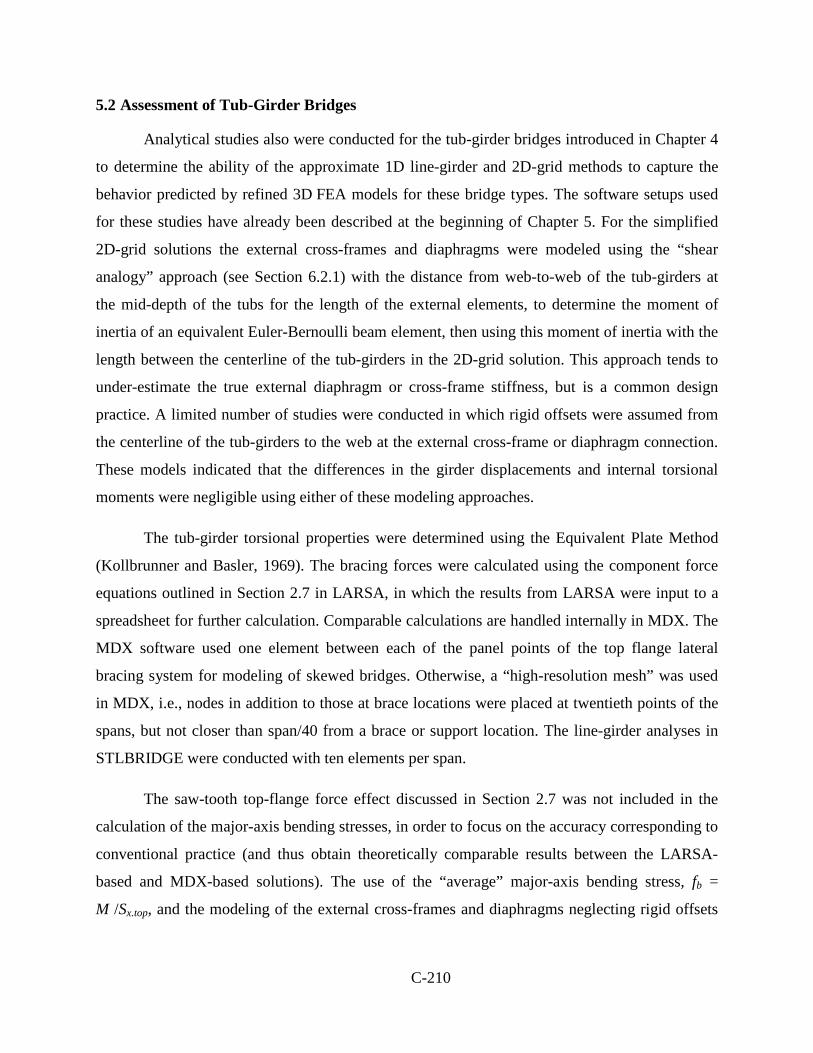
C-210

5.2 Assessment of Tub-Girder Bridges

Analytical studies also were conducted for the tub-girder bridges introduced in Chapter 4

to determine the ability of the approximate 1D line-girder and 2D-grid methods to capture the

behavior predicted by refined 3D FEA models for these bridge types. The software setups used

for these studies have already been described at the beginning of Chapter 5. For the simplified

2D-grid solutions the external cross-frames and diaphragms were modeled using the “shear

analogy” approach (see Section 6.2.1) with the distance from web-to-web of the tub-girders at

the mid-depth of the tubs for the length of the external elements, to determine the moment of

inertia of an equivalent Euler-Bernoulli beam element, then using this moment of inertia with the

length between the centerline of the tub-girders in the 2D-grid solution. This approach tends to

under-estimate the true external diaphragm or cross-frame stiffness, but is a common design

practice. A limited number of studies were conducted in which rigid offsets were assumed from

the centerline of the tub-girders to the web at the external cross-frame or diaphragm connection.

These models indicated that the differences in the girder displacements and internal torsional

moments were negligible using either of these modeling approaches.

The tub-girder torsional properties were determined using the Equivalent Plate Method

(Kollbrunner and Basler, 1969). The bracing forces were calculated using the component force

equations outlined in Section 2.7 in LARSA, in which the results from LARSA were input to a

spreadsheet for further calculation. Comparable calculations are handled internally in MDX. The

MDX software used one element between each of the panel points of the top flange lateral

bracing system for modeling of skewed bridges. Otherwise, a “high-resolution mesh” was used

in MDX, i.e., nodes in addition to those at brace locations were placed at twentieth points of the

spans, but not closer than span/40 from a brace or support location. The line-girder analyses in

STLBRIDGE were conducted with ten elements per span.

The saw-tooth top-flange force effect discussed in Section 2.7 was not included in the

calculation of the major-axis bending stresses, in order to focus on the accuracy corresponding to

conventional practice (and thus obtain theoretically comparable results between the LARSA-

based and MDX-based solutions). The use of the “average” major-axis bending stress, fb =

M /Sx.top, and the modeling of the external cross-frames and diaphragms neglecting rigid offsets

C-211

from the centerline of the tub-girders reflect conventional analysis modeling standards of care in

professional bridge design practice.

In the following, the normalized mean errors from Eq. (5.1) are presented for the major-

axis bending stresses, vertical displacements and girder torsional moments obtained for the 18

tub-girder bridges studied in the NCHRP 12-79 research. However, for the assessment the

analysis accuracy for the top flange lateral bracing (TFLB) and internal cross-frame (CF) axial

forces, the signed errors for the maximum response are reported. In many designs, it is common

to use the same size bracing members along the length of the bridge since this minimizes the

detailing efforts and reduces the possibility of construction errors. As such, the top flange lateral

bracing and cross-frame components are designed for the maximum axial forces found

throughout the length of the bridge. Due to this practice, it is useful to assess the accuracy of the

bracing forces by reporting the signed error for the maximum response for each of the different

types of components. Furthermore, due to some of the subsequent simplified calculations being

substantially conservative, it is useful to reference the signed error to convey that information.

The sign on the error is positive for conservative estimates and unconservative for negative

estimates. The reporting of these errors is grouped by: (1) the top flange lateral bracing

diagonals, (2) the internal cross-frame diagonals, and (3) the combined top flange lateral bracing

struts and internal cross-frame top chords.

Table 5.7 compares the program P1 and P2 2D-grid estimates as well as the1D analysis

estimates for the major-axis bending stresses and vertical displacements to the predictions

obtained from the geometric nonlinear elastic 3D FEA benchmarks. In the table, fb is the major-

axis bending stress, Δz is the vertical displacement and T is the torsional moment. A mean error

is calculated for each response on each girder of the bridges. The values reported by Table 5.7

are the largest mean errors determined by inspecting the values obtained for each girder in a

given bridge. The differences between the linear and geometric nonlinear 3D FEA were

negligible and therefore are not shown. The torsional moments results were not obtained from

program P2 and therefore the accuracy of the results are not evaluated for this case.

C-212

Table 5.7. Tub-girder bridge percent normalized mean errors compared to geometric nonlinear elastic 3D FEA for major-axis bending stresses (fb), vertical displacements (∆z)

and torsional moment (T).

Group Bridge Name

2D-Grid – P1 2D-Grid – P2 1D fb ∆z T fb ∆z fb ∆z T µe µe µe µe µe µe µe µe

C

NTSCR1 7 5 5 12 13 10 6 7 NTSCR2 5 3 6 8 9 8 4 11 NTSCR5 8 6 8 19 10 12 8 11 NTCCR1 5 2 6 8 6 7 4 14 ETCCR15 5 2 20 6 3 7 3 26 XTCCR8 5 3 23 7 3 8 12 27 ETCCR14 6 2 12 36 11 17 8 13 NTCCR5 6 3 3 8 4 6 2 5

S

XTCSN3 3 2 19 5 5 6 6 23 NTSSS1 4 5 31 11 7 5 1 18 NTSSS4 4 1 30 6 5 7 3 53 NTSSS2 8 7 27 19 13 11 5 10 ETSSS2 5 2 28 10 2 9 7 30

C&S

NTSCS5 7 6 3 21 13 12 7 14 NTSCS29 7 7 3 15 11 9 4 9 ETCCS5a 10 6 22 5 5 6 5 29 ETCCS6 6 2 43 22 3 7 2 33

NTCCS22 5 4 3 8 8 6 3 11

In Table 5.7 and in the following discussions, the tub-girder bridges are divided into three

groups based on their geometry: curved radially-supported bridges (labeled as “C”), straight and

skewed structures (labeled as “S”) and curved and skewed bridges (labeled as “C&S”). The

connectivity index, IC, does not apply to tub-girder bridges. This index is primarily a measure of

the loss of accuracy in I-girder bridges due to the poor modeling of the I-girder torsion

properties. For tub-girder bridges, the conventional St. Venant torsion model generally works

well as a characterization of the response of the pseudo-closed section tub-girders. Hence, IC is

not used for characterization of tub-girder bridges in Table 5.7. Furthermore, there is only a weak

correlation between the accuracy of the simplified analysis calculations and the skew index IS for

tub-girder bridges. Therefore, the skew index is not used to characterize tub-girder bridges in

Table 5.7 either. Important differences in the simplified analysis predictions do exist, however,

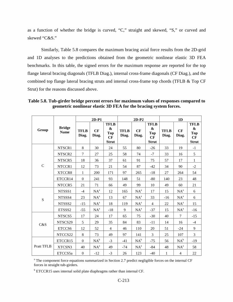
C-213

as a function of whether the bridge is curved, “C,” straight and skewed, “S,” or curved and

skewed “C&S.”

Similarly, Table 5.8 compares the maximum bracing axial force results from the 2D-grid

and 1D analyses to the predictions obtained from the geometric nonlinear elastic 3D FEA

benchmarks. In this table, the signed errors for the maximum response are reported for the top

flange lateral bracing diagonals (TFLB Diag.), internal cross-frame diagonals (CF Diag.), and the

combined top flange lateral bracing struts and internal cross-frame top chords (TFLB & Top CF

Strut) for the reasons discussed above.

Table 5.8. Tub-girder bridge percent errors for maximum values of responses compared to geometric nonlinear elastic 3D FEA for the bracing system forces.

Group Bridge Name

2D-P1 2D-P2 1D

TFLB Diag.

CF Diag.

TFLB &

Top CF

Strut

TFLB Diag.

CF Diag.

TFLB &

Top CF

Strut

TFLB Diag.

CF Diag.

TFLB &

Top CF

Strut

C

NTSCR1 8 30 24 55 80 -26 33 19 -1 NTSCR2 7 27 25 58 74 -7 33 16 5 NTSCR5 18 36 37 61 91 75 57 17 1 NTCCR1 12 73 21 54 87 -42 34 90 -2 XTCCR8 1 200 171 97 265 -18 27 264 54 ETCCR14 0 241 93 148 51 -80 140 23 48 NTCCR5 21 71 66 49 99 10 49 60 21

S

NTSSS1 -4 NAa 12 165 NAa 17 15 NAa 6 NTSSS4 23 NAa 13 67 NAa 33 -16 NAa 6 NTSSS2 -15 NAa 18 119 NAa 4 22 NAa 15 ETSSS2 -55 NAa -18 9 NAa -37 15 NAa -16

C&S

NTSCS5 17 24 17 65 75 -30 40 7 -15 NTSCS29 5 29 35 84 83 -11 14 16 -4 ETCCS6 12 52 4 46 110 20 51 -24 9

NTCCS22 8 73 49 97 141 3 25 107 3

Pratt TFLB ETCCR15 0 NAb -3 -41 NAb -75 56 NAb -19 XTCSN3 40 NAa 49 -74 NAa -84 48 NAa 58 ETCCS5a 0 -12 -3 26 123 -40 1 4 22

a The component force equations summarized in Section 2.7 predict negligible forces on the internal CF forces in straight tub-girders. b ETCCR15 uses internal solid plate diaphragms rather than internal CF.

C-214

An additional group is shown in Table 5.8 corresponding to the bridges that had a Pratt

TFLB system. The simplified analysis methods generally have more difficulty in accurately

predicting the bracing forces for these bridges.

5.2.1 Accuracy of the Vertical Displacements, Major-Axis Bending Stresses and Torsional Moments

Upon inspection of the results corresponding to Table 5.7, the following important trends

can be observed:

Second-Order Amplification

The results obtained from the first-order 3D FEA show that the response amplifications

due to second order effects are negligible for all the tub-girder bridges. Steel tub-girders

generally have as much as 100 to more than 1000 times the torsional stiffness of a comparable I-

girder section. Therefore, when steel tub girders are fabricated with proper internal cross-frames

to restrain their cross-section distortions as well as a proper top flange lateral bracing (TFLB)

system, which acts as an effective top flange plate creating a pseudo-closed cross-section with

the commensurate large torsional stiffness, second-order amplification is rarely of any

significance even during lifting operations and early stages of the steel erection.

2D-Grid Solutions

Based on Table 5.7, several observations can be made regarding the 2D-grid solutions for

the major-axis bending stresses, vertical displacements and torsional moments:

• The 2D-grid solutions from program P1 give better estimates than program P2 for the

major-axis bending stresses and vertical displacements in all the cases in Table 5.7 with

the exception of ETCCS5a. The ETCCS5a bridge uses a Pratt TFLB. The larger errors in

the estimates for this bridge are due to the internal behavior associated with the bracing

system (e.g., the Pratt TFLB system is not symmetric about the centerline of the tub-

girders). Without knowing the details of the internal implementation in program P2, no

conclusions can be drawn to confirm that program P2 has better accuracy for bridges

using Pratt TFLB systems.

• There is no clear distinction in the results for the major-axis bending stresses and vertical

displacements for the different groups “C”, “S” or “C&S”. This means that there is no

C-215

clear effect of curvature or skew on the accuracy of the major-axis bending stresses or

vertical displacements in the simplified tub-girder bridge analysis solutions.

• Only the torsional moments from program P1 were collected. The errors are the largest

for the “S” bridges. However, the groups “C” and “C&S” also have errors that are

comparable to those of the “S” group.

• The torsional moment estimates for bridges ETCCR15 and XTCCR8 exhibit the largest

errors in the “C” group. ETCCR15 has an irregular TFLB layout using Pratt trusses. The

orientation of the TFLB diagonals varies throughout the bridge length. These

characteristics (i.e., the non-symmetry relative to the centerline of the tub-girders and the

variation in the orientations along the length) are believed to induce a behavior difficult

to estimate by simplified 2D and 1D analysis methods. There is no clear reason why the

solutions differed for bridge XTCCR8.

• The torsional results are reasonably accurate for three of the “C&S” bridges. The bridge

ETCCS5a has large errors. This appears to be due again to the use of a Pratt TFLB

system. The bridge ETCCS6 exhibits very large errors in the simplified analysis methods.

The reason for this behavior appears to be the lack of external diaphragms at its inter-

mediate pier.

• The torsional moment estimates for the “S” group exhibit errors larger than group

“C&S”. The “C&S” group bridges have smaller errors even when the independent effects

of skew are expected to be comparable to those on the “S” group. However, the effects of

curvature are large enough to reduce the relative differences. The reason for the reduced

accuracy in the “S” bridges is explained below.

The diaphragm modeling is believed to be an important reason for the lack of accuracy in

the internal torsional moments from the 2D-grid analyses. As noted previously, the 2D-grid

approach used in the NCHRP 12-79 analytical studies tends to under-estimate the cross-frame or

diaphragm stiffnesses. However, it appears that these components behave almost rigidly in many

cases due to the small aspect ratio and the stiffening of the diaphragms. Nevertheless, as noted

previously, a limited number of studies were conducted in which rigid offsets were assumed

from the centerline of the tub-girders to the web at the external cross-frame or diaphragm

connection. These models indicated that the differences in the girder displacements and internal

C-216

torsional moments were negligible using either of these modeling approaches. Therefore, the

results collected in the NCHRP 12-79 research are still inconclusive with respect to this

consideration.

In addition, the internal bracing response appears to influence the accuracy of the

simplified methods in predicting the internal torsional moments. The bridges that are expected to

be subjected to constant internal torsional moments exhibited a slightly nonlinear distribution of

the internal torques. It appears that the variation of the internal torques from a constant value is

related to the TFLB strut lateral forces which follow a similar distribution. The shape also

suggests possible correlation with the girder major-axis bending moment or the strut forces

induced by major-axis bending. It should be noted that constant total internal torques taken by

the full bridge cross-section can be obtained by simple statics in some of these bridges, given the

bridge support reactions. The requirement of constant total internal torque on the full bridge

cross-section is satisfied. However, the individual girders themselves do not exhibit constant

internal torques along their lengths. The reader is referred to Jimenez Chong (2012) for a detailed

assessment of the internal torsion estimates from the simplified methods.

Other errors are attributed to the discretization level of the bridge model; however, these

errors are considered minor compared to the effects discussed above.


The 1D line-girder results in Table 5.7 exhibit the following characteristics:

• The vertical displacements and major-axis bending stress solutions are reasonably good

for all the bridges and are comparable to the corresponding 2D-grid results.

• For the “S” and “C&S” bridges, the 1D line-girder solutions for the vertical

displacements and major-axis bending stresses exhibit better accuracy than the

conventional 2D-grid program P1 solutions in the majority of the cases; however, there is

no clear reason why the line-girder analysis solutions are better for these cases.

• The torsional moment errors from the line-girder analyses are less than or equal to 14 %.

The torsional moment estimates for the ETCCR15, XTCCR8, ETCCS5a and ETCCS6

bridges appear to exhibit larger errors for the same reasons discussed previously

regarding the 2D-grid solution accuracy.

C-217

• Similar to the 2D-gird solutions above, the torsional moment estimates for the “S” group

exhibited errors larger than those from the “C&S” group. The internal bracing behavior is

expected to cause these errors as explained previously; however, an additional reason for

the reduced accuracy in the “S” bridges is explained below.

Additional errors in the line-girder analyses are attributed to the effects of the external

intermediate cross-frames, since the 1D method is unable to capture any information about the

transverse load paths in the bridge system through these components. The external intermediate

cross-frames transfer forces between girders that modify the major-axis bending moments,

torsional moments, and shears in the girders. When skewed external intermediate cross-frames

are used, the cross-frames connect at different relative girder lengths resulting in additional

transferred force between the girders, since the relative vertical displacements that these cross-

frames control are expected to be larger. The effects of external intermediate cross-frames are

again more noticeable in straight bridges since the effect in curved bridges is relatively small

when compared to the overall combined torques from the curvature and skew.

5.2.2 Accuracy of Bracing Forces

2D Grid Solutions

As with the vertical displacements and major-axis bending stresses, the 2D-grid solutions

from program P1 give better estimates than program P2 for the top flange lateral bracing

diagonals forces (TFLB Diag.), internal cross-frame diagonal forces (CF Diag.) and the

combined top flange lateral bracing strut and internal cross-frame top strut (TFLB & Top CF

Strut) for the majority of the cases in Table 5.8. The larger errors in program P2 are attributed to

the coarser discretization used for skewed bridges and the internal process for the evaluation of

the bracing forces. Since the internal process for program P2 is proprietary, there is no

information to confirm the specific differences in the component force calculations between

programs P1 and P2. Therefore, only the results from program P1, which explicitly use the

component force equations, are discussed below.

The following observations can be drawn from the program P1 results in Table 5.8:

• The TFLB diagonal forces directly depend on the major-axis bending and torsional

moments and, consequently, the errors are larger for the “S” group where the torsional

C-218

responses are estimated less accurately. For the “C” and “C&S” bridges, the accuracy is

improved and the estimates are all conservative. The accuracy is affected largely by the

accuracy of the torsional moment estimates. The large negative error for bridge ETSSS2

of -55 % is related to the complex internal forces generated by the interior pier supports

oriented at a significant skew angle in this bridge without any cross-frames or

diaphragms along this bearing line.

• The interior intermediate cross-frame diagonal force estimates show large conservative

errors for the “C” and “C&S” groups. These forces are negligible for the “S” group, and

therefore, these errors are not addressed. The interior intermediate cross-frame diagonal

forces are assumed to depend only on the distortional components of the applied loads

(Fan and Helwig, 2002). The largest distortional contribution is the M/Rh distributed

lateral load which is characterized by the major-axis bending moments. Since the major-

axis bending stresses are captured accurately by the program P2, it is concluded that the

conservative estimates in the above forces are caused by the assumption that the internal

cross-frames provide the only resistance to cross-section distortion (i.e., zero resistance to

cross-section distortion from the girder cross-section itself).

• The combined TFLB & top cross-frame strut force estimates exhibit large conservative

errors for the majority of the bridges, with the exception of the bridges that use a Pratt

TFLB system. These bracing forces depend on a combination of the major-axis bending

moment and torsional moments. The “S” group exhibits smaller errors for these forces.

This result is believed to be related to the reduced accuracy of the torsional moment

estimates for these bridges.

• Additional localized errors are attributed to the interaction of the external intermediate

cross-frames and the internal cross-frames. At the locations that align to the external

intermediate cross-frames there is a transverse load path that the component force

equations do not consider. This effect causes force increases in the adjacent bracing

components.

The bracing force estimates exhibit larger errors than the flange major-axis bending and

vertical displacement estimates for the majority of the cases. However, many of these errors are

conservative. For bridges using Pratt TFLB layouts, the component force equations exhibit a

C-219

poorer performance caused by the interaction between these bracing components and the rest of

the structural system.


The 1D line-girder solutions for the bracing component forces in Table 5.8 exhibit larger

errors than the corresponding responses provided by the program P1 2D-grid solution. These

errors are a consequence of the effects discussed previously in Section 5.2.1. Additional errors

are caused by the discretization level used in the 1D line-girder implementation, which results in

some of the bracing component forces not being calculated based on their actual positions, but

rather based on the closest tenth point.

The following sections synthesize the analysis errors using a grading scheme similar to

the one presented in Section 5.1 for I-girder bridges.

5.2.3 Synthesis of Errors in Major-Axis Bending Stresses and Vertical Displacements for Tub-Girder Bridges

Table 5.9 shows the number of tub-girder bridges within specific ranges of the

normalized mean errors for the major-axis bending stresses and the vertical displacements based

on Table 5.7. Both of the 2D-grid programs P1 and P2 are considered, as well as the 1D analysis

results. The specific selected error ranges are assigned letter grades based on the criteria

described previously for I-girder bridges.

The highlighted rows in Table 5.9 are used to generate simplified scores for each of the

bridge groups and analysis methods in Tables 5.10 and 5.11. The letter grades provided in Table

5.10 correspond to the worst-case scores in Table 5.9, whereas the grades in Table 5.11

correspond to the most frequently occurring score, i.e., the mode score.

Overall, one can observe the following from Tables 5.10 and 5.11:

• For the major-axis bending stresses and vertical displacements, the 2D-grid program P1

and the 1D line-girder analysis get worst-case grades of B and A. The mode of the grades

for these analysis solutions is predominantly an A.

C-220

• For the major-axis bending stresses and vertical displacements, the 2D-grid program P2

gets worst-case grades of F and C. The mode of the grades in these categories is

predominantly a B.

• For the torsional moments, the 2D-grid program P1 and 1D line-girder analysis have

worst-case grades of F. However, the mode of the grades in these categories is a B for the

1D analysis of the “C&S” and “C” bridges and an A for the 2D-grid results. The “S”

bridges have the lowest mode grades in general, D for the 2D-grid P1 solution and F for

the 1D line-girder analysis solution.

Table 5.9. Number of tub-girder bridges within specified error ranges for major-axis bending stress and vertical displacement for each of the types of bridges considered.

Table 5.10. Tub-girder bridge worst-case scores for major-axis bending stress, vertical displacements, and torques.

2D-P1 2D-P2 1D 2D-P1 2D-P2 1D 2D-P1 1DA: ≤ 6% 6 1 1 8 4 5 5 1B: 7-12% 2 5 6 0 3 3 1 3C: 13-20% 0 1 1 0 1 0 1 2D: 21-30% 0 0 0 0 0 0 1 2F: >30% 0 1 0 0 0 0 0 0A: ≤ 6% 4 2 2 4 3 4 0 0B: 7-12% 1 2 3 1 1 1 0 1C: 13-20% 0 1 0 0 1 0 0 1D: 21-30% 0 0 0 0 0 0 3 1F: >30% 0 0 0 0 0 0 2 2A: ≤ 6% 2 1 2 4 2 4 3 0B: 7-12% 3 1 3 1 2 1 0 2C: 13-20% 0 1 0 0 1 0 0 1D: 21-30% 0 2 0 0 0 0 1 1F: >30% 0 0 0 0 0 0 1 1

Number of Bridges within Error RangeGirder Torques

Error range Major-Axis Bending Stress Vertical Displacement

C & S 5

5

C 8

Type of Bridge

S

Number of bridges

2D-P1 2D-P2 1D 2D-P1 2D-P2 1D 2D-P1 1DS B C B B C B F F

C B F C A C B D DC&S B Fa Cb B C B F F

a Modified from D to F based on the score for the C bridgesb Modified from B to C based on the score for the C bridges

Worst-Case ScoresTorqueType of Bridge Major-Axis Bending Stress Vertical Displacement

C-221

Table 5.11. Mode of tub-girder bridge scores for major-axis bending stress, vertical displacements, and torques.

5.2.4 Synthesis of Errors in Bracing Forces for Tub-Girder Bridges

Table 5.12 categorizes the bracing force errors in a manner similar to Table 5.9.

However, in this table, the numbers are collected for both positive (conservative) and for

negative (unconservative) errors. Several of the estimated bracing forces fall into F grades. The

errors are affected significantly by the low accuracy of the torque estimates. However, the

majority of the estimates fall into the conservative categories meaning that the simplified

methods still provide usable estimates for these cases.

5.2.5 Generalized Tub-Girder Bridge Analysis Scores

Tables 5.13 and 5.14 give the generalized analysis scores for the various tub-girder

bridge responses corresponding to the traditional 2D-grid and 1D-line girder methods at large.

Table 5.13 addresses the accuracy of the calculations for major-axis bending stresses, girder

torques, vertical displacements, and girder layovers at the bearings, whereas Table 5.14

addresses the accuracy of the calculations for the top flange lateral bracing, internal cross-frames

and flange lateral bending stresses.

Tables 5.13 and 5.14 are derived by using just the grades from program P1 as being

representative of the true accuracy of 2D-grid methods. Clearly, there was a measurable decrease

in the overall accuracy of the 2D-grid solutions for the tub-girder bridges obtained with program

P2 compared to program P1. Furthermore, the research team had greater control over the

procedures, as well as more detailed information regarding the specifics of the calculations, with

program P1.

2D-P1 2D-P2 1D 2D-P1 2D-P2 1D 2D-P1 1DS A B B A A A D FC A B B A A A A B

C&S B D B A B A A B

TorqueMode of Scores

Type of Bridge Major-Axis Bending Stress Vertical Displacement

C-222

Table 5.12. Number of tub-girder bridges within specified error ranges for the maximum values of the bracing system forces for each of the types of bridges considered.

Type of Bridge

Number of Bridges Error Range

Number of Bridges within Error Range

TFLB Diag.

TFLB & Top CF Strut

CF Diag.

2D-P1

2D-P2

1D

2D-P1

2D-P2 1D 2D-P1 2D-P2 1D

C 7

+F: >30%

0

7

6

4

1

2

5

7

3 +D: 21-30%

1

0

1

3

0

1

2

0

1

+C: 13-20%

1

0

0

0

0

0

0

0

3 +B: 7-12%

3

0

0

0

1

0

0

0

0

+A: ≤ 6%

2

0

0

0

0

2

0

0

0 -A: ≤ 6%

0

0

0

0

0

2

0

0

0

-B: 7-12%

0

0

0

0

1

0

0

0

0 -C: 13-20%

0

0

0

0

1

0

0

0

0

-D: 21-30%

0

0

0

0

1

0

0

0

0 -F: >30%

0

0

0

0

2

0

0

0

0

S 4

+F: >30%

0

3

0

0

1

0

+D: 21-30%

1

0

1

0

0

0

+C: 13-20%

0

0

2

2

1 1

+B: 7-12%

0

1

0

1

0

0

+A: ≤ 6%

0

0

0

0

1

2

-A: ≤ 6%

1

0

0

0

0

0

-B: 7-12%

0

0

0

0

0

0

-C: 13-20%

1

0

1

1

0

1

-D: 21-30%

0

0

0

0

0

0

-F: >30%

1

0

0

0

1

0

C&S 4

+F: >30%

0

4

2

2

0

0

2

4

1 +D: 21-30%

0

0

1

0

0

0

2

0

0

+C: 13-20%

1

0

1

1

1

0

0

0

1 +B: 7-12%

2

0

0

0

0

1

0

0

1

+A: ≤ 6%

1

0

0

1

1

1

0

0

0 -A: ≤ 6%

0

0

0

0

0

1

0

0

0

-B: 7-12%

0

0

0

0

1

0

0

0

0 -C: 13-20%

0

0

0

0

0

1

0

0

0

-D: 21-30%

0

0

0

0

1

0

0

0

1 -F: >30%

0

0

0

0

0

0

0

0

0

Pratt TFLB 3

+F: >30%

1

0

2

1

0

1

+D: 21-30%

0

1

0

0

0

1

+C: 13-20%

0

0

0

0

0

0

+B: 7-12%

0

0

0

0 0

0

+A: ≤ 6%

2

0

1

0

0

0

-A: ≤ 6%

0

0

0

2

0

0

-B: 7-12%

0

0

0

0

0

0

-C: 13-20%

0

0

0

0

0

1

-D: 21-30%

0

0

0

0

0

0

-F: >30% 0 2 0 0 3 0

C-223

Table 5.13. Generalized tub-girder bridge scores for girder major-axis bending stresses, torques, and displacements.

In Tables 5.13 and 5.14, there are several cases where the letter grade for the

“C&S” bridges was lowered from the result derived from Table 5.12 because a grade for

a “C” or an “S” bridge was lower. The table footnotes indicate when these modifications

were made. It should be noted that in Table 5.13, the “C&S” mode scores of A and B for

the prediction of the internal torques by the 2D-grid and the 1D line-girder solutions are

not modified. This is because the torque due curvature is typically much larger than the

torque due to skew, and the contribution of the torque due to curvature tends to be

estimated more accurately in general.

Key observations that can be drawn from Tables 5.13 and 5.14 are as follows:

2D-P1 1D-Line Girder


S B B A BC B C A B

C&S B Cb B BS F F D FC D D A B

C&S F F A BS B B A AC A B A A

C&S B B A AS B B A AC NAa NAa NAa NAa

C&S B B A A

b Modified from B to C based on the score for the C bridges.

Worst-Case Scores Mode of Scores

Major-Axis Bending Stresses

Vertical Displacements

Girder Layover at Bearing Lines

Response Geometry

Girder Torques

a Magnitudes should be negligible where properly designed and detailed diapharagms or cross-frames are present.

C-224

Table 5.14. Generalized tub-girder bridge scores for bracing system forces and flange lateral bending stresses.



S D D D CC D F B F

C&S Da F B F

Pratt TFLB System C F A F

S Fb CC -- --

C&S -- --Pratt TFLB System -- --

S C CC F F

C&S F Fc

Pratt TFLB System F F

S C CC -- A

C&S -- CPratt TFLB System D D

S NAd NAd

C F F

C&S F F

Pratt TFLB System -- Fe

S NAd NAd

C -- --C&S -- D

Pratt TFLB System B --S C CC F F

C&S F Fc

S C CC -- A

C&S -- C

c Modified from a B to an F considering the grade for the C bridges.d For straight-skewed bridges, the internal intermediate cross-frame diagonal forces tend to be negligible.e Modified from an A to an F considering the grade for the C and C&S bridges.

b Large unconsevative error obtained for bridge ETSSS2 due to complex framing. If this bridge is considered as an exceptional case, the worst case unconservative error is -15 % for NTSSS2 (grade = C).

a Modified from a C to a D considerting the grade for the C and the S bridges.

Response Sign of Error GeometryWorst-Case Scores Mode of Scores

TFLB Diagonal Force

TFLB & Top Internal CF Strut

Force

Internal CF Diagonal Force

Positive (Conservative)

Negative (Unconservative)







Top Flange Lateral Bending Stress (Warren TFLB Systems)

C-225

Major-Axis Bending Stresses, Vertical Displacements and Girder Layovers

In these categories the worst-case letter grades are dominated by B grades (see

Table 5.13). The 1D line-girder falls into the C grade for the major-axis bending stresses

in C and “C&S” bridges; however, this should be expected as the complexity of three-

dimensional response is not completely represented in the line-girder analysis model. The

mode grades are dominated by A’s, particularly for the vertical displacements. In

summary the simplified analysis methods show good agreement in the prediction of

major-axis bending stresses, vertical displacement and girder layovers. For tub-girder

bridges the lesser accuracy should be expected from the line-girder analysis since the

interaction between the girders cannot be modeled.

Girder Internal Torques

The 2D-grid and 1D-line girder models represent the bridge in terms of idealized

longitudinal and transverse equivalent beams. However, the torsional behavior is

complex since it involves the interaction of numerous components including the support

diaphragms, external intermediate cross-frames, top flange lateral bracing systems, etc.

Consequently, the lack of modeling accuracy of each of these components adds up and

the worst-case estimates fall to an F grade in curved and/or skewed bridges.

The torque behavior is more difficult to predict accurately as the complexity of

the bridge increases. Uniform spacing of internal bracing and of TFLB system panel

points, reduced interaction between adjacent girders by elimination of intermediate

external bracing, and accurate modeling of support diaphragms generally leads to better

torque estimates. Bridges with complex deck geometry, non-uniform brace spacing,

multiple external intermediate cross-frames between girders, skewed supports, large

eccentric vertical loading, etc., should consider the use of 3D FEA to achieve an accurate

representation of the torsional response.

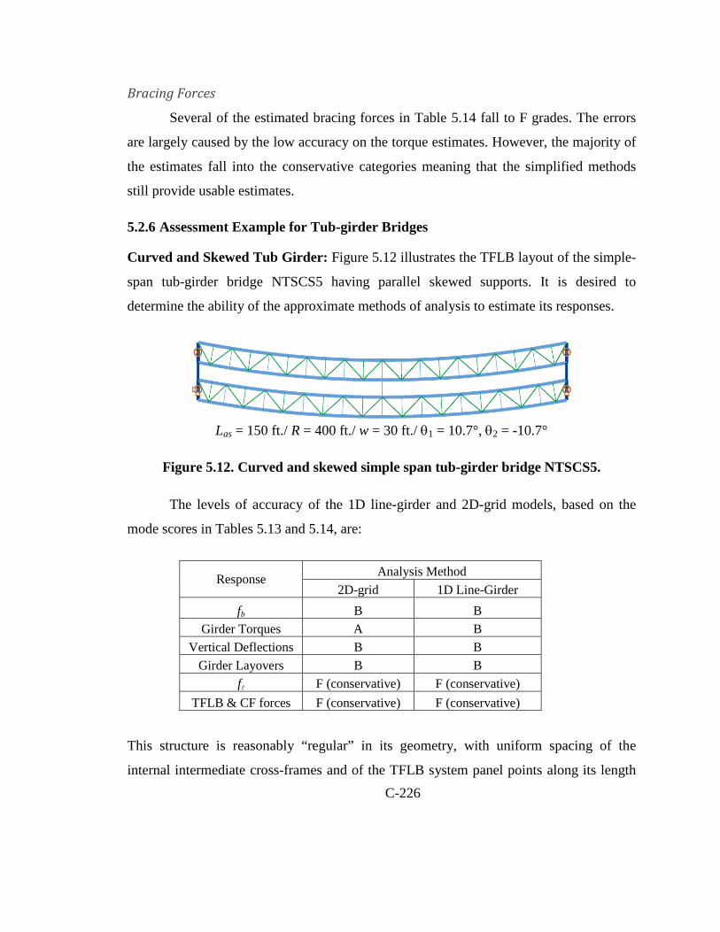
C-226

Bracing Forces

Several of the estimated bracing forces in Table 5.14 fall to F grades. The errors

are largely caused by the low accuracy on the torque estimates. However, the majority of

the estimates fall into the conservative categories meaning that the simplified methods

still provide usable estimates.

5.2.6 Assessment Example for Tub-girder Bridges

Curved and Skewed Tub Girder: Figure 5.12 illustrates the TFLB layout of the simple-

span tub-girder bridge NTSCS5 having parallel skewed supports. It is desired to

determine the ability of the approximate methods of analysis to estimate its responses.

Las = 150 ft./ R = 400 ft./ w = 30 ft./ θ1 = 10.7°, θ2 = -10.7°

Figure 5.12. Curved and skewed simple span tub-girder bridge NTSCS5.

The levels of accuracy of the 1D line-girder and 2D-grid models, based on the

mode scores in Tables 5.13 and 5.14, are:

This structure is reasonably “regular” in its geometry, with uniform spacing of the

internal intermediate cross-frames and of the TFLB system panel points along its length

Response Analysis Method 2D-grid 1D Line-Girder

fb B B Girder Torques A B

Vertical Deflections B B Girder Layovers B B

f F (conservative) F (conservative) TFLB & CF forces F (conservative) F (conservative)

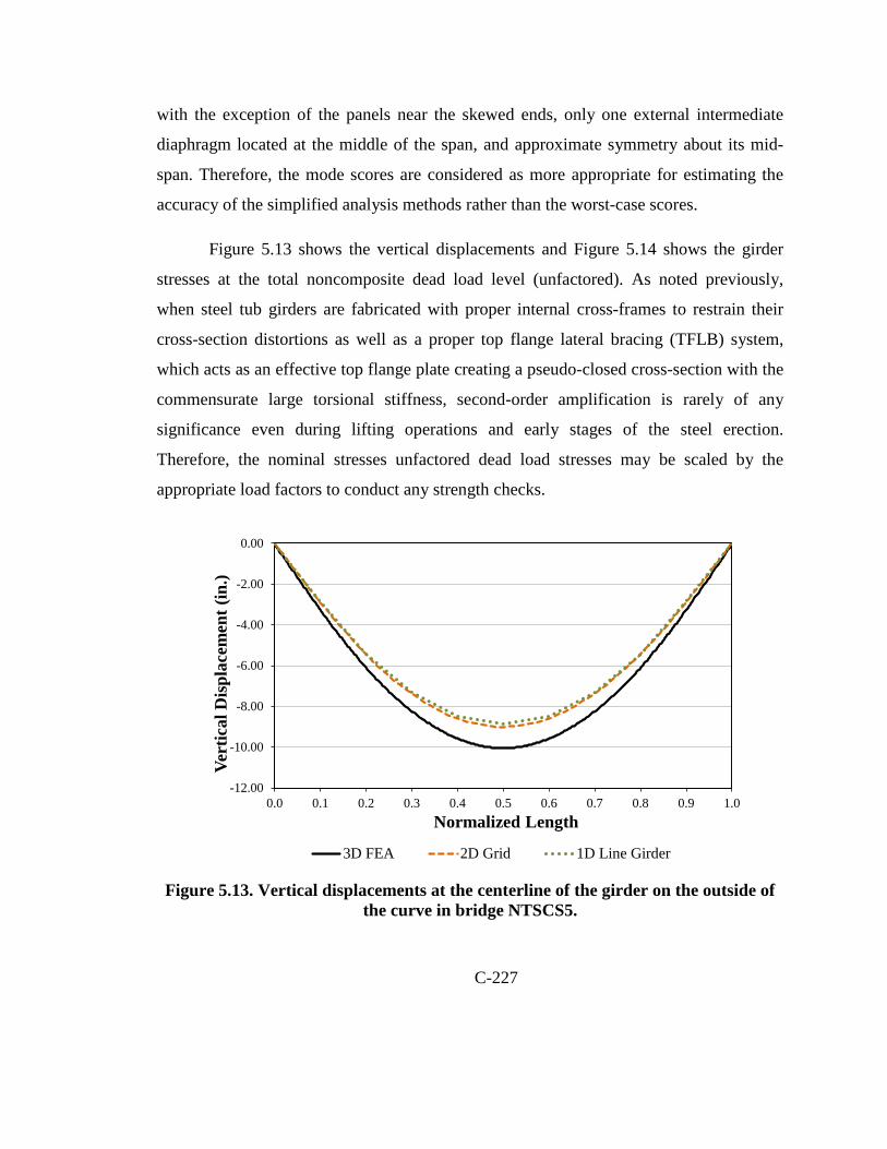
C-227

with the exception of the panels near the skewed ends, only one external intermediate

diaphragm located at the middle of the span, and approximate symmetry about its mid-

span. Therefore, the mode scores are considered as more appropriate for estimating the

accuracy of the simplified analysis methods rather than the worst-case scores.

Figure 5.13 shows the vertical displacements and Figure 5.14 shows the girder

stresses at the total noncomposite dead load level (unfactored). As noted previously,

when steel tub girders are fabricated with proper internal cross-frames to restrain their

cross-section distortions as well as a proper top flange lateral bracing (TFLB) system,

which acts as an effective top flange plate creating a pseudo-closed cross-section with the

commensurate large torsional stiffness, second-order amplification is rarely of any

significance even during lifting operations and early stages of the steel erection.

Therefore, the nominal stresses unfactored dead load stresses may be scaled by the

appropriate load factors to conduct any strength checks.

Figure 5.13. Vertical displacements at the centerline of the girder on the outside of

the curve in bridge NTSCS5.

-12.00

-10.00

-8.00

-6.00

-4.00

-2.00

0.00

0.0 0.1 0.2 0.3 0.4 0.5 0.6 0.7 0.8 0.9 1.0

Vert

ical

Dis

plac

emen

t (in

.)

Normalized Length

3D FEA 2D Grid 1D Line Girder

C-228

Figure 5.14. Flange major-axis and lateral bending stresses on the outside top flange

of the girder on the outside of the curve in bridge NTSCS5.

The top flange lateral bending stresses are estimated conservatively by the 2D-

grid calculations. It should be noted that the 2D-grid curve for these stresses is essentially

just an estimated envelope curve for the maximum flange lateral bending stresses. The

estimated peak flange lateral bending stresses are nearly two times the physical maximum

values, and are not located at the same position as the true peak values. Similar

predictions (not shown) are obtained using the line-girder analysis calculations. Hence,

the grade of F for the top flange lateral bending stresses in Table 5.14 is representative.

The vertical deflections are predicted within a normalized mean error of 6 % by both the

2D-grid and the line-girder analysis in this problem.

Figure 5.15 shows the internal torques predicted in the girder on the outside of the

curve in NTSCS5. It can be observed that the internal torques are predicted very

accurately in this problem, both from the 2D-grid and the 1D line-girder solutions.

Because of the equal and opposite skews at the end bearing lines and the symmetry about

-40.00

-30.00

-20.00

-10.00

0.00

10.00

20.00

30.00

0.0 0.1 0.2 0.3 0.4 0.5 0.6 0.7 0.8 0.9 1.0

fbfl

(ksi)

Normalized Length

3D FEA-fb 2D Grid-fb 1D Line Girder-fb

3D FEA-fl 2D Grid-fl

C-229

the mid-span, the internal torque due to skew is small in this problem. The curvature

effects dominate the total torque. This performance justifies the mode scores of A and B

for prediction of the torques by the simplified analysis solutions. The internal torques are

calculated directly from the structural analysis in the 2D-grid solution. The M/R method

does not provide any estimate of the girder internal torques due to skew. However, as

discussed in Section 2.1.5, the tub-girder internal torques can be estimated reasonably

well for simple, “regular” geometries by considering the major-axis bending responses

from the M/R method along with the assumption that the bearing line diaphragms are

effectively rigid, to calculate the girder relative end twists in each span. The relative end

twists can then be multiplied by the St. Venant torsional stiffness (GJ/L) to obtain an

estimate of the internal torques.

Figure 5.16 shows the axial forces for the TFLB system along the length of the

exterior girder in NTSCS5. To facilitate the visualization of the results the forces are

grouped as positive and negative values, and consecutive results (in every other panel of

the TFLB system) are joined by a line.

Figure 5.15. Internal torques for the girder on the outside of the horizontal curve in

bridge NTSCS5.

C-230

Figure 5.16. Axial forces in the TFLB system diagonals of the girder on the outside of the curve in the NTSCS5 bridge.

One can observe that the overall trends in the predictions from both types of

simplified analysis methods are reasonably good, but that the line-girder analysis results

generally are significantly conservative relative to the 3D FEA benchmarks. This plot

shows that the mode scores of B for the 2D-grid methods are justified, and indicates that

scores better than the mode score (F in this case) are certainly attainable with the line-

girder analysis solutions.

Figure 5.17 shows the predictions from the 2D-grid and 1D line-girder analyses

for the NTSCS5 bridge. Both the 2D-grid and the line-girder analysis predictions appear

to be reasonably good in predicting the overall trends in this case, which may seem to be

at odds with the grade of F for these responses in Table 5.14. However, upon a closer

inspection from Table 5.8, one can observe that the errors in the prediction of the

-250.00

-200.00

-150.00

-100.00

-50.00

0.00

50.00

100.00

150.00

200.00

250.00

0.0 0.1 0.2 0.3 0.4 0.5 0.6 0.7 0.8 0.9 1.0

TFL

B D

iago

nals

Axi

al F

orce

(kip

)

Normalized Length3D FEA-Positive 1D Line Girder-Positive 2D Grid-Positive

3D FEA-Negative 1D Line Girder-Negative 2D Grid-Negative

C-231

maximum forces are + 24 % and +7 % here, whereas these errors are significantly larger

for the other “C&S” bridges.

Figure 5.17. Axial forces in the intermediate internal cross-frame diagonals of the girder on the outside of the horizontal curve in the NTSCS5 bridge.

Figure 5.18 compares the line-girder and 2D-grid analysis results for the axial

forces in the top chord of the intermediate internal cross-frames in the exterior girder of

the NTSCS5 bridge. There are two forces, one on each side of the diagonals, at each

position along the bridge length. The force values at these positions are joined together

by a vertical line, and the values at the adjacent intermediate internal cross-frames are

also connected together by a line to highlight the differences between the two forces. One

can observe that the trends in the maximum force in these components are estimated

reasonable well for this bridge. The maximum force is over-predicted by 17 % in the 2D-

grid solution, whereas this force is predicted quite accurately by the 1D line-girder

analysis solution.

C-232

0.00

5.00

10.00

15.00

20.00

25.00

30.00

35.00

40.00

45.00

0.0 0.1 0.2 0.3 0.4 0.5 0.6 0.7 0.8 0.9 1.0CF

Top

Cho

rd A

xial

For

ce (k

ip)

Normalized Length

3D FEA 1D Line Girder 2D-Grid

Figure 5.18. Axial forces in the top chord of the intermediate internal cross-frames in the exterior girder of the NTSCS5 bridge.

Lastly, Figure 5.19 shows the results for the 2D-grid analysis predictions of the

axial forces in the TFLB struts of the exterior girder for the example bridge. These are the

transverse components in the TFLB system at the locations where there is no

intermediate internal cross-frame. It can be observed that these forces are predicted quite

conservatively by the corresponding component force equations in this case. This is

consistent with the conservative F grade shown for this response for the “C&S” bridges

in Table 5.14.

The reader is referred to Jimenez Chong (2012) for a more comprehensive

summary of example results, similar to the above, from the other tub-girder bridges

studied in the NCHRP 12-79 research.

C-233

Figure 5.19. TFLB strut axial forces in the exterior girder of the NTSCS5 bridge.

C-234

6. Recommended I-Girder Bridge 2D-Grid Analysis Improvements

Chapter 2 provides a broad description of 2D-grid analysis procedures. In the

present chapter, the 2D-grid analysis techniques are studied in more detail. Conventional

methods used in practice to construct a grid model for the analysis and design of steel I-

girder bridges are discussed first to highlight the severe limitations of these approaches.

Next, improved modeling techniques are introduced that can be implemented with

relative ease in 2D-grid analysis software for a better representation of the structural

behavior of I-girder bridges.

6.1 I-Girder Torsional Stiffness for 2D-Grid Analysis

In a thin-walled open-section member, there are two components of torsion

resistance, namely the St. Venant or pure torsion resistance and the flange warping or

non-uniform torsion resistance. Horizontal curvature, support skew, and overhang

eccentric loads subject steel I-girders to torsion. Hence, properly capturing the torsional

properties in a curved and/or skewed steel I-girder bridge is essential to obtain an

accurate prediction of the structure’s performance during construction. Unfortunately, the

conventional approaches commonly used to construct 2D-grid models do not have the

ability to properly represent the torsion properties of I-section girders. Generally, they

only implement the St. Venant torsion component, which results in a substantial

misrepresentation of some of the structural responses of interest during the structure’s

construction.

Consider a beam in cantilever subjected to the external torque, Mz, shown in

Figure 6.1a. Due to the applied torque, the free end of the beam rotates an angle ϕ, and

the flanges displace laterally, where uf = ϕ∙h/2, assuming small rotations, and where h is

the distance between flange centroids. In this member, the total internal torque is equal to

( ) ( ) ( )= +z s wMM z z M z (6.1)

where the first component, Ms, corresponds to the Saint Venant torsion and the second

component, Mw, is the warping torsion. The first component is defined as

C-235

( ) =s GJd

M zdzφ

(6.2)

where G is the steel shear modulus of elasticity and J is the torsion constant of the girder

cross-section. To obtain the warping contribution to the internal torque, one can consider

analyzing the flanges as if they are subjected to lateral bending. The warping torque

along the longitudinal axis of the beam, z, can be decomposed and represented by a force

couple such that Mw(z) = V(z) · h. The forces V(z), which have an opposite sign in each

flange, cause lateral bending of the flanges.

(a) Cantilever beam subject to torque Mz

(b) Decomposition of the warping moment, Mw, in an equivalent force couple

Figure 6.1. Warping torsion in a cantilever beam.

C-236

The governing differential equation for bending in one of the flanges may be used

to determine the flange lateral bending moment, M(z), and the shear force V (z),

( ) ( )( )

2 2

2 2= = -2

ff f

d u z h d zEI EI M z

dz dzφ

(6.3)

( ) ( )3

3= = -2f

dM z h d zV EI

dz dzφ

(6.4)

where E is the modulus of elasticity of the steel, and If is the flange moment of inertia

about the strong axis. Hence, the warping torsion component is

( )3

3= = -w w

d zM V h EC

dzφ

(6.5)

In the above equation, Cw is the warping constant, which is defined as

2

=2w f

hC I (6.6)

The warping constant defined in Eq. (6.6) is valid for doubly-symmetric sections. The

formulae to compute Cw in singly symmetric sections are available in the literature

(Ziemian, 2010). The governing differential equation for a straight I-section girder

subject to torsion is found by substituting Eqs. (6.2) and (6.5) into Eq. (6.1), giving

( )( )3

3= - wz

d d zM z ECG

dzJ

dzφ φ

(6.7)

As shown in Eq. (6.7), the twist angle and the applied torsion moment in an I-section

beam are related through a third order linear differential equation. This equation is not

suitable for implementation using an element with six dofs per node. Hence, an alternate

solution is to ignore the term related to flange warping, and assume that the response is

dominated by St. Venant torsion. With this simplification, the governing differential

equation is reduced to

( ) =z GJd

M zdzφ

(6.8)

C-237

If the applied torque is constant, Eq. (6.8) can be integrated over the beam length (or

bracing points) to obtain a linear relationship between Mz, and ϕ, so that

=z

GJM

Lφ (6.9)

The term GJ/L is the torsional stiffness of the beam ignoring the warping contribution. It

is important to note that the elements used in software packages for modeling of the

girders commonly assume only this contribution to the torsional stiffness.

In box or closed-section members, pure torsion dominates the response, and thus

the warping effects are minor. However, in an I-girder the torsional resistance is

dominated by flange warping. In general, in members with thin-walled open sections, the

effects of warping must be included to properly capture the torsional response. Curved

and skewed steel I-girder bridges are inherently subjected to torsion. Therefore, the

accuracy of the results obtained from the 2D-grid analysis of a curved and/or skewed

bridge can be influenced by the assumptions considered when representing the girder

torsional stiffness.

6.1.1 Modeling of Warping Contributions via Thin-Walled Open-Section (TWOS) 3D-Frame Analysis

A better representation of the I-girder torsion properties is implemented in some

computer programs via an additional warping dof that is provided at each node of the

beam or frame element, as shown in Figure 2.21 (dofs u7 and u14). Various researchers

have developed elements formulated with 14 dofs that include warping deformations. As

discussed in Section 2.6, these types of elements may be referred to as Thin-Walled

Open-Section (TWOS) 3D-Frame elements. These elements generally provide an accu-

rate representation of the physical behavior of non-composite I-girders subjected to

torsion (Yang and McGuire, 1984; Chang, 2006). However, these types of elements must

be applied cautiously for I-girders in their composite condition (Chang, 2006). This is

because these elements do not account for distortional deformation of an I-girder web

into an S shape. When the deck hardens, it provides substantial restraint to both the lat-

eral displacement and the twist of the top flange. However, the bottom flange is still able

to move due to the web out-of-plane flexibility. Hence, the bottom flange lateral displace-

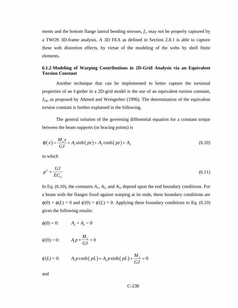
C-238

ments and the bottom flange lateral bending stresses, f, may not be properly captured by

a TWOS 3D-frame analysis. A 3D FEA as defined in Section 2.8.1 is able to capture

these web distortion effects, by virtue of the modeling of the webs by shell finite

elements.

6.1.2 Modeling of Warping Contributions in 2D-Grid Analysis via an Equivalent Torsion Constant

Another technique that can be implemented to better capture the torsional

properties of an I-girder in a 2D-grid model is the use of an equivalent torsion constant,

Jeq, as proposed by Ahmed and Weisgerber (1996). The determination of the equivalent

torsion constant is further explained in the following.

The general solution of the governing differential equation for a constant torque

between the beam supports (or bracing points) is

( ) ( ) ( )1 2 3sinh coshzM zz A pz A pz AGJ

= + + +φ (6.10)

in which

2 =w

GJp

EC (6.11)

In Eq. (6.10), the constants A1, A2, and A3, depend upon the end boundary conditions. For

a beam with the flanges fixed against warping at its ends, these boundary conditions are

ϕ(0) = ϕ(L) = 0 and ϕ'(0) = ϕ'(L) = 0. Applying these boundary conditions to Eq. (6.10)

gives the following results:

ϕ(0) = 0: 2 3+ = 0A A

ϕ'(0) = 0: 1 + = 0zMA p

GJ

ϕ'(L) = 0: ( ) ( )21 cosh sinh 0zMA p pL A p pLGJ

+ + =

and

C-239

1 = - zMA

GJp

( )( )2

cosh 1sinh

z pLMAGJ p pL

−=

( )( )3

cosh 1sinh

z pLMAGJ p pL

−= −

Substituting the constants A1, A2, and A3 in Eq. (6.10), the twist angle in a beam with

warping fixed flanges and subjected to a constant torque is equal to

( ) ( ) ( )( ) ( ) ( )

( )cosh 1 cosh 1

sinh coshsinh sinh

z z z zpL pLM z M M Mz pz pzGJ GJ GJ p pL GJ p pL

− −= − + −φ (6.12)

From the above equation, the relative twist between the beam ends is

( ) ( )( ) ( ) ( )

( )sinh cosh 1 cosh 1

coshsinh sinh

z pL pL pLM L pLGJ p p pL p pL

− −= − + ⋅ −

φ (6.13)

or

zeq

LMGJ

=φ

(6.14)

where Jeq is the equivalent torsion constant for the case where flange warping is fully

fixed at the beam ends, defined as

( ) ( )( ) ( ) ( )

( )

( ) ( )( )

( )

12

1sinh cosh 1 cosh 1

1 coshsinh sinh

cosh 1sinh1

sinh

eq fx fx

pL pL pLJ J pL

pL pL pL pL pL

pLpLJ

pL pL pL

−

−

−

− −= − + ⋅ −

− = − +

(6.15)

With the equivalent torsion constant, Jeq(fx-fx), it is possible to simulate the

torsional stiffness of an I-girder with warping-fixed ends. This equivalent torsion constant

may be substituted into the grid model to capture more properly the girder properties.

C-240

The above derivation can be used to model the torsional rigidity of the interior

girder segments, which are the segments defined between two intermediate cross-frames.

At the girder ends, the flanges typically are free to warp. For the end segments, defined

between the end and the first intermediate cross-frame, the equivalent torsion stiffness

may be determined assuming that the warping boundary conditions are fixed-free at the

segment ends. In this case, the boundary conditions necessary to determine the constants

A1, A2, and A3 are ϕ(0) = ϕ(L) = 0 and ϕ''(0) = ϕ'(L) = 0. Applying these boundary

conditions to Eq. (6.10) gives the following results:

ϕ(0) = 0: 2 3+ = 0A A

ϕ''(0) = 0: 22 = 0A p

ϕ'(L) = 0: ( )1 cosh 0zMA p pLGJ

+ =

and

( )11

coshzMA

GJ p pL= −

32 0A A= =

Substituting these constants in Eq. (6.10), the rotation angle in a beam with free-fixed

warping conditions subject to a constant torque is equal to

( ) ( )( )

sinhcosh

z z pzM z MzGJ GJ p pz

= −φ (6.16)

and

( )( )

sinh1

coshz pLM L

GJ pL pL

= −

φ (6.17)

C-241

Therefore, for an exterior girder segment, the equivalent torsion constant is equal to

( )( )( )

1sinh

1cosheq fr fx

pLJ J

pL pL

−

−

= −

(6.18)

This implementation of the equivalent torsion constant provides a simple method

to approximate the overall torsional stiffness of I-girders. For the analysis of an I-girder

bridge, Jeq is calculated taking L as the distance between cross-frames. Then the torsion

constant J is defined in the program using the calculated value of Jeq. With this technique,

the typical 12-dof frame element available in commercial programs can be used to

construct traditional 2D-grid models that are a closer representation of the physical

structure than models constructed using conventional practices, where the flange warping

contributions are neglected.

Even though the use of the equivalent torsion constant represents a potential

improvement for 2D-grid modeling techniques, there is a limitation that has to be

considered. In reality, warping is not fully fixed at the girder bracing points (i.e., the

relative flange lateral bending rotations are not zero at the cross-frame positions). In a

particular flange segment, which is defined by the distance between bracing points,

warping restraint is provided by the adjacent segments. In reality, at the segment ends,

the flange warping resembles a partially restrained condition. Unfortunately, it is not

practical to provide further guidelines on how to determine the equivalent torsion

coefficient other than assuming fixed-fixed warping for interior girder segments and free-

fixed for the end segments. In general, it is not feasible to capture the girder torsional

stiffness exactly unless the actual flange warping displacements at the nodes of the

analysis model are known. However, the response predictions obtained from analyses of

bridges with challenging geometries and complex bracing systems with equivalent

torsion constants calculated based on fixed-fixed and pinned-fixed warping conditions are

significantly more accurate than the responses obtained from analyses that ignore the

warping contributions (Sanchez, 2011).

C-242

Another factor to consider is the calculation of the equivalent torsion constant for

different girder segments in the structure. The distance between cross-frames varies

depending on how the engineer configures the bracing system in the bridge. As shown in

Figure 6.2, cross-frames may be provided at one or both sides of the girder, and the

distance between them is not necessarily the same. In the figure, Segments 2 and 3 have

different unbraced lengths. Therefore a different equivalent torsion constant must be

determined for each segment. In a skewed bridge, different unbraced lengths are common

near the skewed supports. Therefore, it is necessary to compute a Jeq for each of the

different unbraced lengths.

Figure 6.2. Definition of unbraced length for computation of the effective torsion

constant, Jeq.

6.2 Cross-Frame Element Stiffnesses

In this section, the modeling techniques used to represent the cross-frames in 2D-

grid analyses are studied. First, the conventional practices are presented and analyzed,

emphasizing their accuracy and their limitations to represent the physical behavior of the

cross-frames in the bridge. Next, two-node elements that capture the physical behavior of

the X-type, V-type and inverted V-type cross-frames are developed and implemented in

LARSA 4D (LARSA, 2010), a software system commonly used for design of steel bridges.

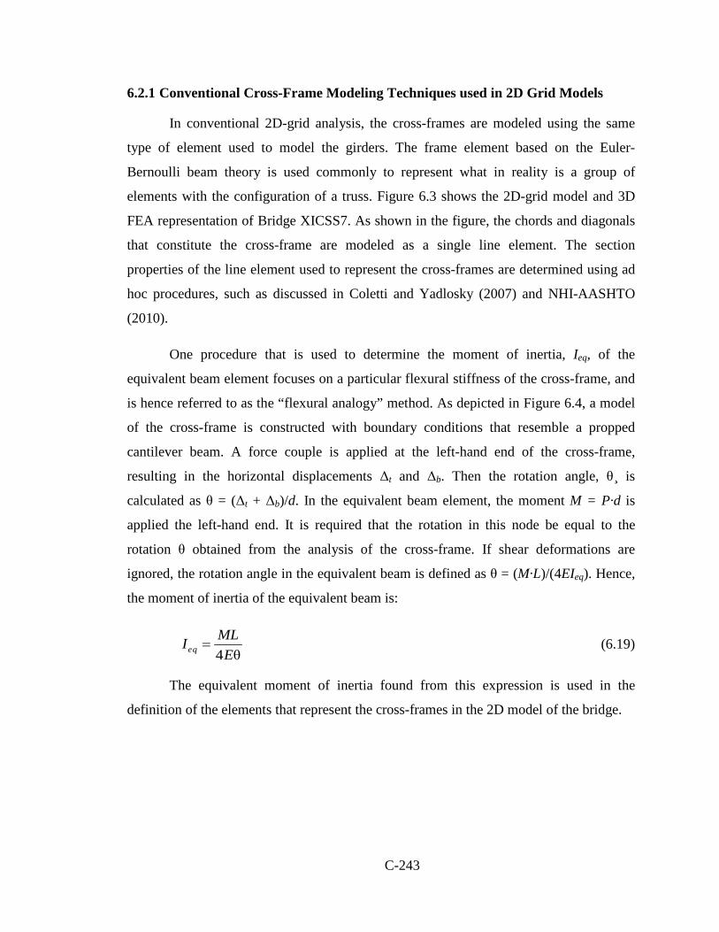
C-243

6.2.1 Conventional Cross-Frame Modeling Techniques used in 2D Grid Models

In conventional 2D-grid analysis, the cross-frames are modeled using the same

type of element used to model the girders. The frame element based on the Euler-

Bernoulli beam theory is used commonly to represent what in reality is a group of

elements with the configuration of a truss. Figure 6.3 shows the 2D-grid model and 3D

FEA representation of Bridge XICSS7. As shown in the figure, the chords and diagonals

that constitute the cross-frame are modeled as a single line element. The section

properties of the line element used to represent the cross-frames are determined using ad

hoc procedures, such as discussed in Coletti and Yadlosky (2007) and NHI-AASHTO

(2010).

One procedure that is used to determine the moment of inertia, Ieq, of the

equivalent beam element focuses on a particular flexural stiffness of the cross-frame, and

is hence referred to as the “flexural analogy” method. As depicted in Figure 6.4, a model

of the cross-frame is constructed with boundary conditions that resemble a propped

cantilever beam. A force couple is applied at the left-hand end of the cross-frame,

resulting in the horizontal displacements Δt and Δb. Then the rotation angle, θ¸ is

calculated as θ = (Δt + Δb)/d. In the equivalent beam element, the moment M = P·d is

applied the left-hand end. It is required that the rotation in this node be equal to the

rotation θ obtained from the analysis of the cross-frame. If shear deformations are

ignored, the rotation angle in the equivalent beam is defined as θ = (M·L)/(4EIeq). Hence,

the moment of inertia of the equivalent beam is:

4 θeqMLIE

= (6.19)

The equivalent moment of inertia found from this expression is used in the

definition of the elements that represent the cross-frames in the 2D model of the bridge.

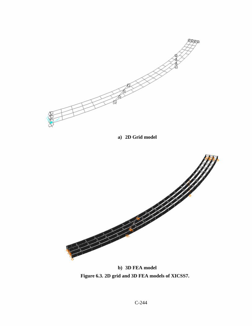
C-244

a) 2D Grid model

b) 3D FEA model

Figure 6.3. 2D grid and 3D FEA models of XICSS7.

C-245

Figure 6.4. Flexural analogy model used in conventional practice to find the moment of

inertia of the equivalent beam (adapted from Coletti and Yadlosky (2007)).

Another approximate procedure used to determine the moment of inertia of the

equivalent beam elements is the “shear analogy” method. As depicted in Figure 6.5, in

this method, the cross-frame is modeled with boundary conditions that allow only the

vertical displacement of one of the ends. The force P is applied at the end that is free to

move and the vertical deflection is captured. In the equivalent beam, the deflection due to

this load is equal to Δ = (PL3)/(12EIeq). Therefore, the moment of inertia used in the 2D-

grid models to represent the cross-frames based on this method is:

3

12eqPLI

E=

∆ (6.20)

These procedures are highly approximate. It is clear that for a cross-frame, two

substantially different equivalent moments of inertia can be obtained, depending on

which model is used. Both the flexural analogy and shear analogy methods only capture a

part of the structural behavior of the cross-frames and are not necessary a realistic

representation of these bridge components.

C-246

Figure 6.5. Shear analogy model used in conventional practice to find the moment of

inertia of the equivalent beam (adapted from Coletti and Yadlosky (2007)).

In many cases, the responses predicted by 2D models constructed using the above

procedures are close to the benchmark solutions obtained from 3D FEA analyses. As

shown in (Sanchez, 2011), even for bridges with complex geometries, the approximate

representation of the cross-frames often does not result in significant differences with

respect to the 3D FEA predictions. In particular, the major-axis bending responses of the

girders obtained from 2D-grid models constructed with these standard practices are often

a close representation of the benchmark solutions. The reason for this incongruence is

that in many cases, the cross-frame in-plane rigidity is much larger than the girder

torsional rigidity of the I-girders.

The response affected the most by modeling the cross-frames with these ad hoc

procedures is the internal forces in the cross-frame elements. In addition, the cross-frame

forces generally have a significant influence on the flange lateral bending responses in I-

girder bridges. To properly capture the flow of the transverse forces that results from

horizontal curvature and support skew and the associated lateral bending response of the

girders, it is necessary to perform the analysis with a more realistic model of the cross-

frames. If the cross-frame forces are not computed accurately, it is not possible to obtain

an accurate prediction of the f stresses, either.

C-247

The practices used to model the cross-frames along with the poor representation

of the torsion stiffness of the I-girders are the most significant limitations of the

traditional methods used to conduct 2D-grid analysis. In the next section, simple two-

node elements that are a more realistic representation of the cross-frame contributions to

the system behavior are developed.

6.2.2 Improved Representation of the Cross-Frames in 2D-Grid Models

In the conventional methods commonly used to model the cross-frames, the

structural properties of these components are not properly captured. It is evident that to

overcome the limitations of the equivalent beam elements used to model the cross-

frames, it is required to capture more efficiently their contributions to the system

response. This can be done by applying the direct stiffness method to a model of the

physical cross-frame and recovering the coefficients that constitute its stiffness matrix.

For this purpose, consider the X-type cross-frame depicted in Figure 6.6a and its line

element representation. For simplicity only the in-plane representation (3-dof per node) in

shown in the figure. If the connection plates are assumed to be rigid, and the rotational

continuity is neglected at the element connections in the plane of the cross-frame, it is

possible to apply unit displacements to each of these dofs to recover the stiffness

coefficients as shown in Figure 6.6b. Since in the cross-frame plane the chords and the

diagonals are simply connected, the coefficients depend exclusively on the axial stiffness

of the cross-frame elements. Note that for the formulation of the stiffness matrix, it is

necessary to consider that the top chord, bottom chord, and the diagonals can have

different cross-sections, i.e., different areas, At, Ab, Ad1, and Ad2, respectively. It is

important to formulate the two-node element considering these characteristics, so it can

handle cases such as cross-frames without top-chords (i.e., At = 0), or with only one

diagonal (i.e., Ad1 or Ad2 = 0). The generality of an element formulated considering

different element cross-sections is also beneficial when modeling bearing line cross-

frames. The top-chord of these cross-frames generally has a larger section than the rest of

the elements since it supports the deck joint.

C-248

Physical Cross-Frame Two-Node Element Representation

a) Reduction of the physical cross-frame to a two-node element

b) Unit displacements for the determination of the stiffness matrix coefficients

Figure 6.6. Determination of the stiffness matrix to represent the X-type cross-frame with a two-node beam element.

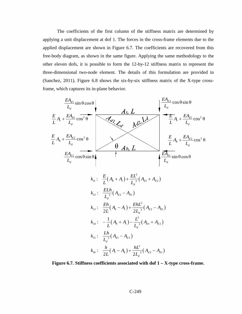
C-249

The coefficients of the first column of the stiffness matrix are determined by

applying a unit displacement at dof 1. The forces in the cross-frame elements due to the

applied displacement are shown in Figure 6.7. The coefficients are recovered from this

free-body diagram, as shown in the same figure. Applying the same methodology to the

other eleven dofs, it is possible to form the 12-by-12 stiffness matrix to represent the

three-dimensional two-node element. The details of this formulation are provided in

(Sanchez, 2011). Figure 6.8 shows the six-by-six stiffness matrix of the X-type cross-

frame, which captures its in-plane behavior.

( ) ( )

( )

( ) ( )

( ) ( )

( )

( ) ( )

3

2

3

1 2

2

11 1 2

12 2 13

2

13 13

2

14 1 2

15 3

2

3 216 1

:

:

:

:

:

:

2 2

1

2 2

b t d dd

d dd

b t d dd

b t d dd

d dd

d dd

t b

E ELk A A AL LELhk AL

Eh EhLk A A AL L

Lk A A AL L

Lhk AL

h hLk A A A

A

A

L

A

A

A

AL

++ +

+ −

−

−

−

−

− +− +

+ −

Figure 6.7. Stiffness coefficients associated with dof 1 – X-type cross-frame.

21 cos θdt

d

EAE AL L

+

2 2cos θdb

d

EAE AL L

+

21 cos θdt

d

EAE AL L

+

2 2cos θdb

d

EAE AL L

+

2 cosθsin θd

d

EAL

1 sin θ cosθd

d

EAL

2 cosθsin θd

d

EAL

1 sin θ cosθd

d

EAL

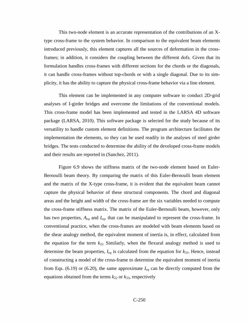
C-250

This two-node element is an accurate representation of the contributions of an X-

type cross-frame to the system behavior. In comparison to the equivalent beam elements

introduced previously, this element captures all the sources of deformation in the cross-

frames; in addition, it considers the coupling between the different dofs. Given that its

formulation handles cross-frames with different sections for the chords or the diagonals,

it can handle cross-frames without top-chords or with a single diagonal. Due to its sim-

plicity, it has the ability to capture the physical cross-frame behavior via a line element.

This element can be implemented in any computer software to conduct 2D-grid

analyses of I-girder bridges and overcome the limitations of the conventional models.

This cross-frame model has been implemented and tested in the LARSA 4D software

package (LARSA, 2010). This software package is selected for the study because of its

versatility to handle custom element definitions. The program architecture facilitates the

implementation the elements, so they can be used readily in the analyses of steel girder

bridges. The tests conducted to determine the ability of the developed cross-frame models

and their results are reported in (Sanchez, 2011).

Figure 6.9 shows the stiffness matrix of the two-node element based on Euler-

Bernoulli beam theory. By comparing the matrix of this Euler-Bernoulli beam element

and the matrix of the X-type cross-frame, it is evident that the equivalent beam cannot

capture the physical behavior of these structural components. The chord and diagonal

areas and the height and width of the cross-frame are the six variables needed to compute

the cross-frame stiffness matrix. The matrix of the Euler-Bernoulli beam, however, only

has two properties, Aeq and Ieq, that can be manipulated to represent the cross-frame. In

conventional practice, when the cross-frames are modeled with beam elements based on

the shear analogy method, the equivalent moment of inertia is, in effect, calculated from

the equation for the term k22. Similarly, when the flexural analogy method is used to

determine the beam properties, Ieq is calculated from the equation for k33. Hence, instead

of constructing a model of the cross-frame to determine the equivalent moment of inertia

from Eqs. (6.19) or (6.20), the same approximate Ieq can be directly computed from the

equations obtained from the terms k22 or k33, respectively

C-251

( ) ( ) ( ) ( ) ( ) ( ) ( ) ( ) ( ) ( )

( ) ( ) ( ) ( ) ( ) ( )

( )

2 2 2 21 2 2 1 1 1 2 13 3 3 3

2 2 2 22 1 1 2 1 2 1 2 1 2 1 23 3

1 12 1 2 23 32 2

3 3 3 3

2 2

2 2

2

L Lh h hL L Lh h hA A A A A Ab t d d d d b t d d b t d d d d d dd d d d d d

A A A A A Ad d d

LA A A A A A A A A A A A A At bL

d d d d d d d d

L L LL L L L L L

Lh h h L Ld

d d d d d d

Ab t

h h h LA A A A A AL L L L L L

h AL

k E

++ + + − − + −− + −

−

+

=

− + − −

− + + − + +

− ( ) ( ) ( ) ( ) ( ) ( ) ( ) ( ) ( )

( ) ( ) ( ) ( ) ( ) ( ) ( )

2 2 2 2 22 1 24 2 42 2 4 2 2 4

1 11 23

2 2 2 2 21 1 2 1 2 1 2 1 23 3 3 3 3 3

2 2 21 2 1 2 1 3332

223

A A A A A A Ad d d d b t d d t b d d d d b thL h L h h L h hL h L h h LA A A A A A A A A A A

L L LL L L L L L

L Lh h hL L LhA A A A A A A A A A AL L LL L

d dd d d d d d

A A A Ab t d d d d t b d d b t d d dLd Ld dLd d

+ + − + +− + + + − − − + +

− + − +− +− + ++ − ( ) ( ) ( )

( ) ( ) ( ) ( ) ( ) ( )

( ) ( ) ( ) ( ) ( ) ( ) ( )

1 22 2

1

22 1 3

2 2 2 21 2 1 2 2 1 1 2 1 23 3 3 3 3 3

2 2 2 2 2 2 21 1 2 1 23

22 2

2 1 22 4 22 2 23 3234

h hLA A AtL L

Lh h h L Lh h h LA A A A A A

A Ad b d dd

A A A A A Ad d d d d d d d d d d dd d d d d d

A A A A Ad d d d

L L L L L L

hb t

hL h L h h L h hL h LA A A A A A A Ad d b d dd d d d

At b tL dL LL L L L L

+ −

− − −

− −

− + + − + +

− + − − + − −+ ++ +− ( ) ( ) ( )4 4

2 2 21 2 1 23 3

h h LA A Ad d b t d dL dA A A

L

+ ++ +

Figure 6.8. Two-node element stiffness matrix, two-dimensional representation of the X-type cross-frame.

( ) ( )0 0 0 0

12 6 12 60 0

6 4 6 20 0

0 0 0 0

12 6 1

3 3:11

3 2 3 2

2 2

3 2 3 2

2

2 60 0

6 22

6 40 0

eq eqeq b t d d

eq eq eq eq

eq eq eq eq

eq eq

eq eq eq eq

eq eq eq

A Ak A A A L L A

L LI I I I

L L L LI I I I

L LL Lk EA A

L LI I I I

L L L LI I I I

L LL L

eq

= + +− − − = − − − −

−

( )

( )( )

( )( ) ( )( )

( )( ) ( )( )

( )( )

( )( )

( )( ) ( )( )

( )( ) ( )( )

1 23: 012 2 1

3: 013 130 216 1

2 3:22 1 22 3 3:23 1 22 2 3 3: 1633 1 2

2

22 2 22: 2 2

3 12

1

2

2

16

83 3: 836 1 2

k Lh L A

k h L A hL L A A

k A hL L A At b

k h L L A

Ad

Ad d d

Ab t d d d

h L A d d d

I Aeq d d d

I Aeq d d d

I h A L Aeq b t d d d

I h A L A

k h L L A

eq b t d d d

k A h L A

k A h L A

+ −

+

= −

= −

= − + −

+ +

+ +

= +

= +

= +

= − +

Figure 6.9. Comparison of the stiffness matrices of the X-type cross-frame and the Euler-Bernoulli beam.

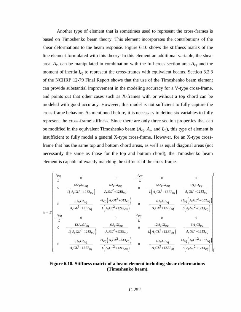
C-252

Another type of element that is sometimes used to represent the cross-frames is

based on Timoshenko beam theory. This element incorporates the contributions of the

shear deformations to the beam response. Figure 6.10 shows the stiffness matrix of the

line element formulated with this theory. In this element an additional variable, the shear

area, Av, can be manipulated in combination with the full cross-section area Aeq and the

moment of inertia Ieq to represent the cross-frames with equivalent beams. Section 3.2.3

of the NCHRP 12-79 Final Report shows that the use of the Timoshenko beam element

can provide substantial improvement in the modeling accuracy for a V-type cross-frame,

and points out that other cases such as X-frames with or without a top chord can be

modeled with good accuracy. However, this model is not sufficient to fully capture the

cross-frame behavior. As mentioned before, it is necessary to define six variables to fully

represent the cross-frame stiffness. Since there are only three section properties that can

be modified in the equivalent Timoshenko beam (Aeq, Av, and Ieq), this type of element is

insufficient to fully model a general X-type cross-frame. However, for an X-type cross-

frame that has the same top and bottom chord areas, as well as equal diagonal areas (not

necessarily the same as those for the top and bottom chord), the Timoshenko beam

element is capable of exactly matching the stiffness of the cross-frame.

( ) ( )( )

( )( )

( )

0 0 0 0

12 6 12 60 0

2 22 212 1212 12

2 24 3 2 66 60 0

2 22 212 1212 12

A A

L LA GI A GI A GI A GIv v v v

A GL EI A GL EIL A GL EI L A GL EIv eq v eqv eq v eq

I A GL EI I A GL EIeq v eq eq v eqA GI A GIv v

A GL EI A GL EIL A GL EI L A GL EIv eq v eq

eq eq

eq eq e

v e

q eq

e

q v eqk E

q eq

eqA

−

−+ ++ +

+ −−

+ ++ +=

−

( ) ( )( )

( )( )

( )

0 0 0 0

12 6 12 60 0

2 22 212 1212 12

2 22 6 4 36 60 0

2 22 212 1212 12

eq

eq eq eq eq

e

A

L LA GI A GI A GI A GIv v v v

A GL EI A GL EIL A GL EI L A GL EIv eq v eqv eq v eq

I A GL EI I A GL EIeq v eq eq v eqA GI A GIv v

A GL EI A GL EIL A GL EI L A GL EIv eq v eqv eq v

q eq

eq

− − −+ ++ +

− +−

+ ++ +

Figure 6.10. Stiffness matrix of a beam element including shear deformations (Timoshenko beam).

C-253

The above discussion shows that neither the Euler-Bernoulli beam nor the

Timoshenko beam have the characteristics required for an exact representation of general

X-type cross-frames. The two approximate methods used in conventional practice (i.e.,

the flexural analogy method and the shear analogy method) yield different cross-frame

properties that capture only one part of the cross-frame behavior. Therefore, the

equivalent beam concept generally is not an accurate representation of the structural

behavior of these components. This section illustrates the development of the two-node

element for the X-type cross-frame. Sanchez (2011) also discusses the development of

the V-type and inverted V-type cross-frames, which are other configurations commonly

used for girder bridges. For these types of cross-frames, the Timoshenko beam element is

not able to capture the exact physical stiffness properties. The most significant errors in

the approximation are for V-type cross-frames without a top chord, where the cross-

frame flexural stiffness is critically dependent upon the characteristics of the bottom

chord and the connection plates in the vicinity of the joint at the cross-frame mid-length.

The two-node equivalent beam elements developed by (Sanchez, 2011) can be

implemented in any computer program used to conduct 2D-grid analyses. In the NCHRP

12-79 research, these elements were implemented in the LARSA 4D program since this

software facilitates the inclusion of user-defined elements. However, the cross-frame

two-node elements can be implemented in other programs that have user-defined

elements, or by software developers, with minor effort.

6.3 Cross-Frame Forces

In 2D-grid models, the primary analysis output is the joint displacements. These

displacements are multiplied by the corresponding element stiffness coefficients to

calculate the joint forces. To obtain the forces in the chords and diagonals of the cross-

frames, the joint forces commonly are decomposed as shown in Figure 6.11. The Vi and

Vj shears are essentially the same; the difference between them is equal to the weight of

the cross-frame. This effect is negligible, so the largest of these forces is typically

selected and equally divided between the top and bottom nodes of the cross-frame

(assuming an X-type cross-frame). In most of the other cross-frame types, a single

diagonal frames into the girders at each end of the cross-frame, and therefore, the shear

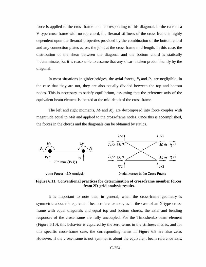
C-254

force is applied to the cross-frame node corresponding to this diagonal. In the case of a

V-type cross-frame with no top chord, the flexural stiffness of the cross-frame is highly

dependent upon the flexural properties provided by the combination of the bottom chord

and any connection plates across the joint at the cross-frame mid-length. In this case, the

distribution of the shear between the diagonal and the bottom chord is statically

indeterminate, but it is reasonable to assume that any shear is taken predominantly by the

diagonal.

In most situations in girder bridges, the axial forces, Pi and Pj, are negligible. In

the case that they are not, they are also equally divided between the top and bottom

nodes. This is necessary to satisfy equilibrium, assuming that the reference axis of the

equivalent beam element is located at the mid-depth of the cross-frame.

The left and right moments, Mi and Mj, are decomposed into force couples with

magnitude equal to M/h and applied to the cross-frame nodes. Once this is accomplished,

the forces in the chords and the diagonals can be obtained by statics.

Figure 6.11. Conventional practices for determination of cross-frame member forces

from 2D-grid analysis results.

It is important to note that, in general, when the cross-frame geometry is

symmetric about the equivalent beam reference axis, as in the case of an X-type cross-

frame with equal diagonals and equal top and bottom chords, the axial and bending

responses of the cross-frame are fully uncoupled. For the Timoshenko beam element

(Figure 6.10), this behavior is captured by the zero terms in the stiffness matrix, and for

this specific cross-frame case, the corresponding terms in Figure 6.8 are also zero.

However, if the cross-frame is not symmetric about the equivalent beam reference axis,

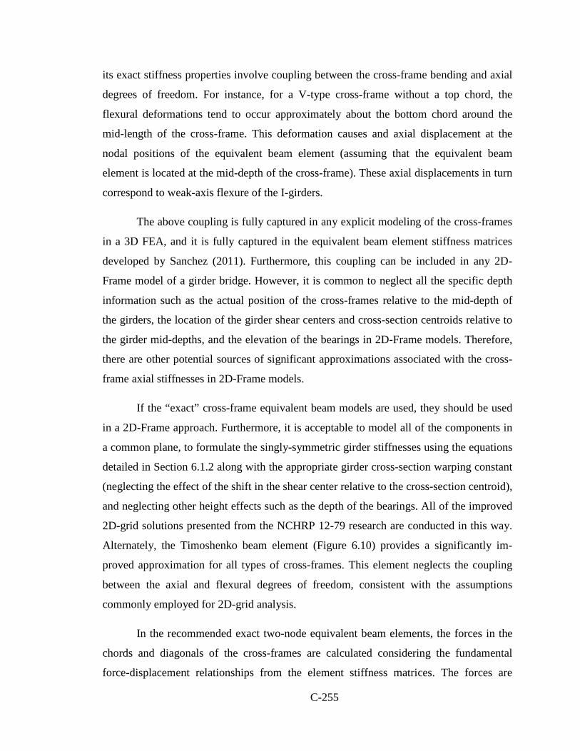
C-255

its exact stiffness properties involve coupling between the cross-frame bending and axial

degrees of freedom. For instance, for a V-type cross-frame without a top chord, the

flexural deformations tend to occur approximately about the bottom chord around the

mid-length of the cross-frame. This deformation causes and axial displacement at the

nodal positions of the equivalent beam element (assuming that the equivalent beam

element is located at the mid-depth of the cross-frame). These axial displacements in turn

correspond to weak-axis flexure of the I-girders.

The above coupling is fully captured in any explicit modeling of the cross-frames

in a 3D FEA, and it is fully captured in the equivalent beam element stiffness matrices

developed by Sanchez (2011). Furthermore, this coupling can be included in any 2D-

Frame model of a girder bridge. However, it is common to neglect all the specific depth

information such as the actual position of the cross-frames relative to the mid-depth of

the girders, the location of the girder shear centers and cross-section centroids relative to

the girder mid-depths, and the elevation of the bearings in 2D-Frame models. Therefore,

there are other potential sources of significant approximations associated with the cross-

frame axial stiffnesses in 2D-Frame models.

If the “exact” cross-frame equivalent beam models are used, they should be used

in a 2D-Frame approach. Furthermore, it is acceptable to model all of the components in

a common plane, to formulate the singly-symmetric girder stiffnesses using the equations

detailed in Section 6.1.2 along with the appropriate girder cross-section warping constant

(neglecting the effect of the shift in the shear center relative to the cross-section centroid),

and neglecting other height effects such as the depth of the bearings. All of the improved

2D-grid solutions presented from the NCHRP 12-79 research are conducted in this way.

Alternately, the Timoshenko beam element (Figure 6.10) provides a significantly im-

proved approximation for all types of cross-frames. This element neglects the coupling

between the axial and flexural degrees of freedom, consistent with the assumptions

commonly employed for 2D-grid analysis.

In the recommended exact two-node equivalent beam elements, the forces in the

chords and diagonals of the cross-frames are calculated considering the fundamental

force-displacement relationships from the element stiffness matrices. The forces are

C-256

computed by recovering the joint displacements to determine the element deformations.

The deformations are then multiplied by the corresponding stiffness coefficients to obtain

the element forces. Applying this criterion, the forces in the chords and the diagonals of

an X-type cross-frame are:

( ) ( )4 1 3 62t

TCE A hF u u u u

L⋅ = − + −

(6.21)

( ) ( )4 1 6 32b

BCE A hF u u u u

L⋅ = − + −

(6.22)

( ) ( ) ( )11 4 1 2 5 3 62 2 2

2d

Dd

E AF L u u h u u Lh u uL⋅

= − + − + + (6.23)

( ) ( ) ( )22 1 4 2 5 3 62 2 2

2d

Dd

E AF L u u h u u Lh u u

L⋅

= − − + − + + (6.24)

where ui is the displacement at dof i. Figure 6.6 shows the dof numbering associated with

the displacements and the orientation of Diagonals 1 and 2. Similar equations for the

computation of the forces in V-type and inverted V-type cross-frames are provided in

(Sanchez, 2011).

6.4 Calculation of I-Girder Flange Lateral Bending Stresses Given Cross-Frame Forces

In a steel I-girder bridge, the flange lateral bending stresses, f , that result from

the horizontal curvature and the skew effects must be considered in the design of the

structure. As required by the AASHTO Bridge Specifications (AASHTO, 2010), these

stresses are combined with the major-axis bending stresses to conduct the strength checks

in the noncomposite and composite structure. However, at present, there is limited

guidance on how to determine the f stresses associated with skew.

In a skewed bridge, the cross-frames induce forces in the I-girders, subjecting

their flanges to lateral bending stresses, f. Currently, the only methods to compute these

cross-frame forces are via refined 3D frame models that explicitly include the warping

stiffness contributions, or via a rigorous 3D FEA. However, with some exceptions, these

C-257

analysis methods are used predominantly for research purposes or for bridges with

particularly complex geometry, since significant effort may be required to construct the

model and post-process the results (many of the emerging software systems provide

substantial reductions in these efforts).

To obtain the flange lateral bending stresses, f , it is necessary to have an accurate

prediction of the cross-frame forces. In the approximate 1D line-girder analysis methods,

the forces in the cross-frames due to the skew are not captured; therefore, it is not feasible

to determine these f stresses with a 1D analysis. Similarly, as shown in the second case

study of Section 5.1.3, due to the poor representation of the cross-frame in-plane

properties and the poor representation of the torsional characteristics of the I-girders, the

2D-grid models developed with conventional techniques often substantially underpredict

the physical cross-frame forces. For these reasons, and in the absence of an alternative

predictor, the AASHTO Bridge Specifications (AASHTO, 2010), Article C6.10.1 pro-

vides the coarse estimates for the flange lateral bending stresses discussed previously in

Chapter 2. Unfortunately, no estimates are provided within the AASHTO Specifications

for the corresponding cross-frame forces.

In this section, a method to estimate the f stresses in straight and skewed bridges

is introduced. Bridge NISSS16 is used to illustrate the calculations. Figure 6.12a shows

the plan view of the bridge. It is intended to capture the flange lateral bending stresses in

the top flange of girder G6. Figure 6.12b shows the free-body diagram of the second

cross-frame in Bay 6, B6-CF2. The cross-frame forces (i.e., FTC, FD1, FD2, and FBC) are

transferred to the girders in the form of nodal forces (A, B, C, and D). The horizontal and

vertical components of the vertical loads are determined by applying the equilibrium

equations at nodes A to D, such that:

C-258

2

2

1

1

2

2

1

1

cos (θ)sin (θ)

cos (θ)sin (θ)

cos (θ)sin (θ)

cos (θ)sin (θ)

x BC D

y D

x TC D

y D

x TC D

y D

x BC D

y D

A F FA FB F FB FC F FC FD F FD F

= − −

= −

= − −

=

= +

=

= +

= −

(6.25)

(a) Plan view of Bridge NISSS16

(b) Forces transferred from cross-frame B6-CF2 to girders G6 and G7

(c) Top flange of girder G6 subject to the horizontal components of the nodal

forces

Figure 6.12. Determination of cross-frame forces as the first step in the calculation of flange lateral bending, top flange of girder G6, NISSS16, at TDL level.

Cx,B5,

CF8 (0.77

)

Cx,B5,

CF7 (-

3.28)

Cx,B5,

CF6 (0.13

)

Cx,B5,

CF5 (10.5

5)

Cx,B5,

CF4 (26.6

7)

Cx,B5,

CF3 (4.16

)

Cx,B5,

CF2 (9.17

)

Bx,B6,

CF9 (0.65

)

Bx,B6,

CF8 (3.28

)

Bx,B6,

CF7 (0.12

)

Bx,B6,

CF6 (-

10.72

Bx,B6,

CF5 (-

25.36

Bx,B6,

CF4 (-

1.83)

Bx,B6,

CF3 (-

8.60)

Bx,B6,

CF2 (-

13.13 Cx,B5,

CF1 (1.77

)

Bx,B6,

CF1 (5.78

)

G1

G9

…

G6

B6-CF2

C-259

where θ is the angle between the chords and the diagonals. Next, the lateral forces Ax and

Bx are converted to statically-equivalent lateral forces at the level of the girder flanges,

based on a girder cross-section free-body diagram. For simplicity of notation, these

converted flange-level forces are referenced using the same symbols in the following.

Given the various flange level forces applied from the cross-frames, the girder

flanges are isolated from the rest of the structure and subjected to the horizontal

components of the nodal forces, as illustrated in Figure 6.12c. Notice that the Cx force

components of the cross-frames in Bay 5 are applied on one side of the flange, while the

Bx components of the Bay 6 cross-frames are applied on the other side. The magnitudes

of the forces acting on the flange under consideration are included in the figure. They are

computed with Eqs. (6.21) to (6.24), by using the cross-frame force estimates obtained

from the improved 2D-grid analysis of this bridge. The 2D-grid model is constructed

following the recommendations discussed in Sections 6.1 and 6.2.

The above nodal lateral forces are the source of the lateral bending in the flange

of girder G6; however, only the forces acting in the region where the cross-frames are

staggered cause large flange lateral bending stresses in bridge NISSS16. As shown in

Figure 6.12c, the forces in the region where the cross-frames are contiguous can be larger

than those where they are staggered, but these lateral forces tend to cancel each other out.

For example, in the intermediate contiguous cross-frame line that is closest to the skewed

support, the forces are 26.67 kips and -25.36 kips, and the resultant is 1.31 kips. Hence,

although the nodal forces are larger than at other locations, the force resultant causes a

minor effect on the flange lateral bending. The cross-frames, and the connections

between the cross-frames and the girders, however, must be designed considering these

forces.

Another important aspect to consider regarding this approximate procedure is that

the nodal lateral forces are not completely balanced in Figure 6.12c. This is because the

girder torsional stiffnesses, upon which the calculation of the cross-frame forces is based,

include a contribution both from the girder warping torsion as well as the girder St.

Venant torsion. As such, a portion of the above forces is transferred (by the interaction of

the flange with the girder web) into the internal St. Venant torsion in the girders. More

C-260

specifically, corresponding small but undetermined distributed lateral forces are trans-

ferred to the flange from the web in Figure 6.12c.

In the case of the flange under consideration, the unbalance calculated by adding

all the lateral forces acting on the flange (including the lateral components of the forces

from the skewed bearing line cross-frames) is -2.58 kips. If the distributed lateral load

transferred from the web is added to the above nodal lateral forces, the flange would be in

equilibrium.

Solutions to this problem include:

(1) Use the girder torsional rotations and displacements along with the detailed open-

section thin-walled beam stiffness model associated with Jeq to directly determine

the flange lateral bending stresses. This results in an imbalance in the flange

lateral bending moments on each side of the intermediate cross-frames (since Jeq

is based the assumption of warping fixity at the cross-frame locations). This

moment imbalance could be re-distributed along the girder flange to determine

accurate flange lateral bending moments. A procedure analogous to elastic

moment distribution could be utilized for this calculation. Although this approach

is a viable one, it is relatively complex. Therefore, it was not pursued in the


(2) Focus on an approximate local calculation in the vicinity of each cross-frame,

utilizing the forces delivered to the flanges from the cross-frames as shown in

Figure 6.12c. Because of its relative simplicity this approach was selected in the


It should be noted that the girder flange lateral bending stresses are calculated directly

and explicitly from the element displacements and stiffnesses in the TWOS 2D-grid and

TWOS 3D-frame solutions. Therefore, these methods provide the best combination of

accuracy and simplicity for the grid or frame element calculation of the flange lateral

bending stresses. However, the disadvantage of this approach is the additional complexity

of the element formulation, and the requirement that an additional warping degree of

freedom has to be included in the global structural analysis.

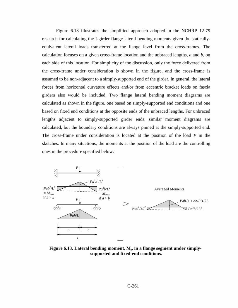
C-261

Figure 6.13 illustrates the simplified approach adopted in the NCHRP 12-79

research for calculating the I-girder flange lateral bending moments given the statically-

equivalent lateral loads transferred at the flange level from the cross-frames. The

calculation focuses on a given cross-frame location and the unbraced lengths, a and b, on

each side of this location. For simplicity of the discussion, only the force delivered from

the cross-frame under consideration is shown in the figure, and the cross-frame is

assumed to be non-adjacent to a simply-supported end of the girder. In general, the lateral

forces from horizontal curvature effects and/or from eccentric bracket loads on fascia

girders also would be included. Two flange lateral bending moment diagrams are

calculated as shown in the figure, one based on simply-supported end conditions and one

based on fixed end conditions at the opposite ends of the unbraced lengths. For unbraced

lengths adjacent to simply-supported girder ends, similar moment diagrams are

calculated, but the boundary conditions are always pinned at the simply-supported end.

The cross-frame under consideration is located at the position of the load P in the

sketches. In many situations, the moments at the position of the load are the controlling

ones in the procedure specified below.

Figure 6.13. Lateral bending moment, M, in a flange segment under simply-

supported and fixed-end conditions.

a b

L

Pab/L

Pa2b/L2Pab2/L2

Pa2b2/L3

= Mmax if a > b

= Mmax if b > a P

P

Pab (1 + ab/L2) /2L

Pa2b/2L2Pab2/2L2

Averaged Moments

C-262

Given the moment diagrams for the above cases, the NCHRP 12-79 research

determined that an accurate to conservative solution for the flange lateral bending

moments and stresses is obtained generally by:

(1) Averaging the above moment diagrams, and

(2) Taking the largest averaged internal moment in each of the unbraced lengths as

the flange lateral bending moment for that length.

This solution is repeated cross-frame location by cross-frame location along the length of

the girders and the largest moment from the two solutions obtained for each unbraced

length is taken as the estimate of the flange lateral bending moment in that unbraced

length. (For the unbraced lengths at girder simply-supported ends, only one solution is

performed.)

The above procedure recognizes that the true flange lateral bending moment is

bounded by the “pinned” and “fixed” moment diagrams (neglecting the small St. Venant

torsional contributions from the interaction with the web) and ensures that the flange

lateral bending moments required for static equilibrium are never underestimated. Also,

the average of the pinned and fixed moment diagrams is analogous to the use of the

approximation qLb2/10 rather than qLb

2/12 when estimating the flange lateral bending

moments due to horizontal curvature, where q is the equivalent flange radial load. In

Figure 6.14 shows the plots of the response predictions obtained using the above

approach and the results obtained from the 3D FEA for the top flange of Girders G3 and

G6. The plots include the responses for fully fixed and simply supported end conditions.

Additionally, a trace that represents the average between these two responses is also

included. As shown in these plots, the estimates obtained with the proposed approach and

using the results derived from the improved 2D-grid model are a reasonable

representation of the benchmark. As expected, the responses predicted by the FEA lay

between the predictions determined assuming fully fixed and pinned ends, and are

accurately estimated by taking the average of the last two predictions.

C-263

Girder G3

Girder G6

Figure 6.14. Flange lateral bending stresses in Bridge NISSS16 at TDL level.

-10.0

-5.0

0.0

5.0

10.0

15.0

20.0

0.00 0.10 0.20 0.30 0.40 0.50 0.60 0.70 0.80 0.90 1.00

f (k

si)

Normalized Length

2D-Pinned 2D-Avg. 2D-Fixed 3D FEA

-15.0

-10.0

-5.0

0.0

5.0

10.0

15.0

0.00 0.10 0.20 0.30 0.40 0.50 0.60 0.70 0.80 0.90 1.00

f (k

si)

Normalized Length

2D-Pinned 2D-Avg. 2D-Fixed 3D FEA

C-264

It should be emphasized that to predict the flange lateral bending stresses using

the proposed method, it is necessary to first have an accurate prediction of the cross-

frame forces. Hence, the results of a 2D-grid analysis conducted with conventional

practices cannot be used for this purpose. The cross-frame forces should be obtained from

an analysis where the recommendations of Sections 6.1 and 6.2 are implemented in the

model.

6.5 . Summary of Proposed Improvements for the Analysis of I-Girder Bridges using 2D-Grid Analysis

The previous sections highlight the characteristics of the 2D-grid models and the

limitations of the conventional techniques to properly represent the behavior of an I-

girder bridge during construction. Essentially, there are two modeling practices that can

considerably affect the accuracy of the analyses. The first practice is related to the

representation of the torsional properties of the I-girders. In computer programs

commonly used for 2D-grid modeling, the torsional resistance of the I-girders is

formulated considering only the pure or St. Venant torsion contributions. The other factor

that can affect the response predictions of a 2D-grid analysis is the model used to

represent the cross-frames. In most of cases, the cross-frames are modeled using an

equivalent beam element, which is based on the Euler-Bernoulli beam theory.

The improved modeling techniques discussed in this chapter can be implemented

with minor effort in design offices. The equivalent torsion constant as a means to

simulate the warping contributions to the girder torsional stiffness is a concept that

requires a simple manipulation of the cross-section properties in the model definition.

This modification, however, can improve the predictions obtained from a grid model of

bridges where the torsional responses have a major role in the structural response, as is

the case of curved and/or skewed bridges.

Similar to the girder torsional properties, a better representation of the cross-

frames can be accomplished by formulating two-node elements that consider all the

stiffness contributions to the system response. The elements developed in the NCHRP

12-79 research were included and tested in the LARSA 4D program since the architecture

of this software allows the inclusion of user defined finite elements. However, the

C-265

element potentially could be implemented in the library of any commercial software used

for bridge engineering.

Finally, it is worth emphasizing on the relevance of an accurate model of cross-

frames and girder torsional stiffness. In many structures, wide fluctuations in cross-frame

stiffness do not have a significant effect in the structural responses. Similarly, in some

cases, the poor torsion model of the girders does not represent a considerable source of

error. The studies conducted in this research show that in straight and skewed bridges

with skew indices below 0.30, torsion induced by skew is minor and the participation of

the cross-frames may be negligible. Hence, bridges of these characteristics are insensitive

to the cross-frame and girder torsional stiffness model. In fact, a line girder analysis may

be sufficient in these cases. However, when the index goes above this limit, due to the

torsion that the girders experience as a result of the transverse load path, the system

becomes more sensitive to the torsion model and changes in the cross-frame stiffness. In

bridges with IS ≥ 0.30, it is important how the torsional girder stiffnesses and the cross-

frame in-plane stiffnesses are represented in the program since they can have a

substantial influence on the system responses.

In curved and skewed bridges it is not clear how the horizontal curvature and the

support skew interact to determine when the structure is sensitive to the cross-frame and

girder torsional stiffness models. For these bridges, the NCHRP 12-79 research shows

that it is difficult to determine limits on when a traditional 2D-grid analysis provides

acceptable results. For these structures it is suggested to implement the approaches

discussed in this chapter to obtain accurate predictions.

C-266

7. Consideration of Locked-In Forces in I-Girder Bridges due to

Cross-Frame Detailing

7.1 Cross-Frame Detailing Methods

Curved and skewed I-girder bridges exhibit significant torsional displacements of the

individual girders and of the overall bridge cross-section. As a result, the girder webs can

be plumb only in one configuration. If the structure is built such that the webs are plumb

in the ideal no-load position, they generally cannot be plumb under the action of the

structure’s steel or total dead load. The deflected geometry resulting from these torsional

displacements can impact the fit up of the members (i.e. come-along and jacking forces),

the erection requirements (crane position and capacities, number of temporary supports

and tie downs), and the bearing cost and type. Furthermore, significant layover (i.e.,

relative lateral deflection of the flanges associated with twisting) can be visually

objectionable. This is particularly the case at piers and abutments.

If the torsional deflections are large enough, then the cross-frames often are detailed

with a lack-of-fit that induces opposing torsional displacements to offset the dead load

torsional rotations. As explained in the AASHTO LRFD Specifications Article C6.7.2

(2010), different types of cross-frame detailing are used to achieve approximately plumb

webs in the theoretically no-load, steel dead load, or total dead load conditions. These

methods are summarized below.

No-Load Fit (NLF): For NLF detailing, the cross-frames are fabricated to fit the girders

in their cambered, plumb, no-load geometry without inducing any locked-in forces (i.e.,

there is no lack-of-fit). Figure 7.1 illustrates the behavior associated with NLF detailing

at a representative intermediate cross-frame in the no-load geometry and under the action

of the dead loads. (Geometric factors such as cross-slope, super-elevation and profile

grade line are not shown in this figure and in the subsequent figures for clarity.) The

cross-frame is assumed to be normal to the girders for purposes of the following

discussion. The girders deflect from their plumb no-load geometry into an out-of-plumb

C-267

position under the action of the dead loads. In Figure 7.1, this twisting of the girders is

driven primarily by the larger vertical deflection of the girder on the right compared to

the one on the left. Since the cross-frame deformation is relatively small within its plane,

the cross-frame induces a twist into the girders due to the differential vertical

displacements.

(a) No-load geometry

(b) Under the action of dead loads

Figure 7.1. Illustration of the behavior associated with No-Load Fit (NLF) detailing at intermediate cross-frames (geometric factors such as cross-slope, super-elevation

and profile grade line are not shown for clarity).

In addition, as explained in Section 2.1.4, the cross-frames at skewed bearing

lines tend to rotate about their own skewed axis and warp (twist) out of their plane.

However, the cross-frame in-plane stiffnesses are again relatively large compared to the

C-268

girder lateral and torsional stiffnesses. Therefore, the girders must lay over at any skewed

bearing line to maintain compatibility with the cross-frames under the dead load rotations

at the bearing line. This is illustrated by Figure 7.2, which is repeated from Figure 2.7 for

ease of reference.

Figure 7.2. Girder top flange deflections and girder rotations at a fixed bearing

location on a skewed bearing line.

The above two sources of girder layover work both jointly and independently.

That is, if the bearing line cross-frames were theoretically taken out, the layovers at the

bearing lines caused by the intermediate cross-frames would be somewhat different (but

generally in the same direction). Similarly, if the bearing line cross-frames were left in

and the intermediate cross-frames taken out, the girder layovers would be different at the

intermediate cross-frame locations, although the direction of the layover tends to be the

same.

Total Dead Load Fit (TDLF): For TDLF detailing, the cross-frames are fabricated to fit

to the girders in their ideal final plumb position under total dead load (that is plumb webs

but with the total dead load vertical deflections subtracted from the initial girder camber).

Figure 7.3 illustrates the behavior associated with TDLF detailing at an intermediate

cross-frame (assumed normal to the girders) before it is connected to girders in the no-

C-269

load geometry, after it is connected to girders in the theoretical no-load position (if the

cross-frames could be connected to the girders without any dead load on the structure),

and under the total dead load. The intermediate cross-frame does not fit-up with the

girder connection points in the no-load geometry since it is fabricated for the final plumb

geometry. Also, as noted above, the cross-frame is relatively stiff in its own plane.

Therefore, the girders, which are relatively flexible, must be twisted in a direction

opposite to their dead load torsional rotations to make the connections to the cross-frame.

However, under the action of the total dead loads, the girder webs rotate back to an

approximately plumb position. The lack-of-fit between the girders and the cross-frame,

due to the differential vertical camber, induces additional locked-in internal stresses and

corresponding deformations in the structure when the girders and cross-frames are forced

together to make their connections.

All of the illustrations of the deflections, rotations and deformations in Figure 7.3

correspond to a generic location within the span. To achieve a web plumb condition

under the total dead load at a skewed bearing line, the opposite of the layover under the

total dead load is applied at this location initially (i.e., due to the initial lack-of-fit). Based

on the assumption that the in-plane cross-frame deformations are relatively small, this is

achieved by fabricating the end cross-frames to fit the final geometry of the girders, but

attaching the cross-frames to the girders in their initial cambered geometry. It is

commonly assumed that the girder end connection plates, which are also the bearing

stiffeners, are vertical in the reference geometry shown in Figure 7.2. Due to the total

dead load camber, the girder end connection plates are rotated by the negative of the total

dead load major-axis bending rotations shown in Figure 7.2 ( –φx ) to achieve the initial

cambered geometry. Correspondingly, if the cross-frames at the bearing line are to be

connected to the girders in the theoretical no-load geometry, the girder top flange must be

laid over by the negative of the dead load layover shown in Figure 7.2 (–∆x). In this work,

the girders are assumed to be fabricated with plumb webs in their initial no-load

geometry. Therefore, the girder top flange in Figure 7.2 must be forced over by –∆x to

make the connection to the bearing line cross-frame in the ideal no-load condition.

C-270

(a) No-load geometry before connecting the cross-frames

(b) No-load geometry after connecting the cross-frames

(c) Under the total dead load

Figure 7.3. Illustration of the behavior associated with Total Dead Load Fit (TDLF) detailing at intermediate cross-frames (geometric factors such as cross-slope, super-

elevation and profile grade line are not shown for clarity).

C-271

When the total dead load has been applied to the structure, the girders “unwind”

under the application of the load such that they come back to an approximately plumb

position in the final constructed configuration. The girders deflect into the approximately

plumb position shown in Figure 7.3(c) at the intermediate cross-frame locations, the

girders rotate approximately back to the plumb reference geometry at the skewed bearing

lines, and the end connection plates (i.e., the bearing stiffeners) rotate approximately back

to the vertical position at the bearings.

Steel Dead Load Fit (SDLF): For SDLF detailing, the cross-frames are fabricated to fit

the girders in their idealized final plumb position under the steel dead load (that is plumb

webs but with the steel dead load vertical deflections subtracted from the initial girder

camber). SDLF detailing is similar to TDLF detailing in that locked-in stresses and

deformations are developed due to a lack-of-fit. However, the lack-of-fit between the

cross-frames and girders in the no-load geometry for SDLF is often smaller than that due

to TDLF. When SDLF is used, the webs rotate back to an approximately plumb position

under the action of the steel dead loads.

7.2 Procedures for Determining Locked-In Forces

As demonstrated in the subsequent sections of this chapter, the locked-in forces in the

bridge system associated with SDLF and TDLF detailing are generally of comparable

magnitude to the corresponding steel or total dead load forces. For example, in a straight-

skewed I-girder bridge constructed with TDLF detailing of the cross-frames, the locked-

in cross-frame forces and girder flange lateral bending stresses are nearly equal and

opposite to the corresponding total dead load values. As such, the final cross-frame forces

and girder flange lateral bending stresses (equal to the sum of the locked-in and total dead

load values) tend to be relatively small. Engineers typically expect this once it is under-

stood that the girders are essentially “reverse twisted” by the initial lack-of-fit associated

with the TDLF detailing, but then they “unwind” back to their plumb geometry under the

total dead loads. Since the girders unwind back to an approximately plumb position under

the total dead load, it is anticipated that the corresponding flange lateral bending stresses

and the cross-frame forces are small.

C-272

When an engineer conducts an accurate 2D-grid analysis using the improvements

discussed in Chapter 6, or an accurate 3D FEA using methods such as those outlined in

Section 2.8.1, one might expect that the corresponding internal cross-frame forces and

girder flange lateral bending stresses are calculated accurately. Unfortunately, if the

cross-frames are detailed for anything other than NLF, the calculated internal distribution

and magnitude of the cross-frame forces and girder flange lateral bending stresses will be

substantially different from the values in the physical bridge. Without the calculation of

the locked-in forces due to the initial lack-of-fit between the cross-frames and the girders,

an accurate 2D-grid or 3D FE analysis captures only the applied dead load effects.

Technically, the inclusion of the lack-of-fit effects from SDLF or TDLF detailing in

analysis is relatively straightforward. Analysis solutions for the locked-in forces

associated with DLF detailing are fundamentally no different than typical lack-of-fit

problems students first solve in undergraduate Strength of Materials; however, the lack-

of-fit due to DLF detailing is generally a 3D geometry problem. One way of capturing the

influence of cross-frame detailing is to construct a full model of any intermediate erection

stage of the bridge with the girders in their initial no-load cambered and plumb positions,

with the cross-frames connected to the girders, and with initial strains introduced into the

cross-frames corresponding to the initial lack-of-fit caused by the cross-frame detailing.

An analysis of this specific stage is then performed by simply including the cross-frame

member initial strains in the analysis and “turning gravity on.”

The initial strains corresponding to the lack-of-fit are introduced to each cross-

frame member. These strains are calculated by using the cross-frame member length in

the final dead load position, which is the fabrication length of the cross-frame members,

(Configuration A) and length between the work points of the girders in the initially-

plumb cambered geometry (Configuration B). Figure 7.4 shows an example intermediate

cross-frame. The differential cambers between the girders often generate large initial

axial strains in the cross-frame members. However, this is not a problem physically, since

the initial strains are just an analytical device to determine the locked-in forces. The

actual strains in the structure are generally much smaller.

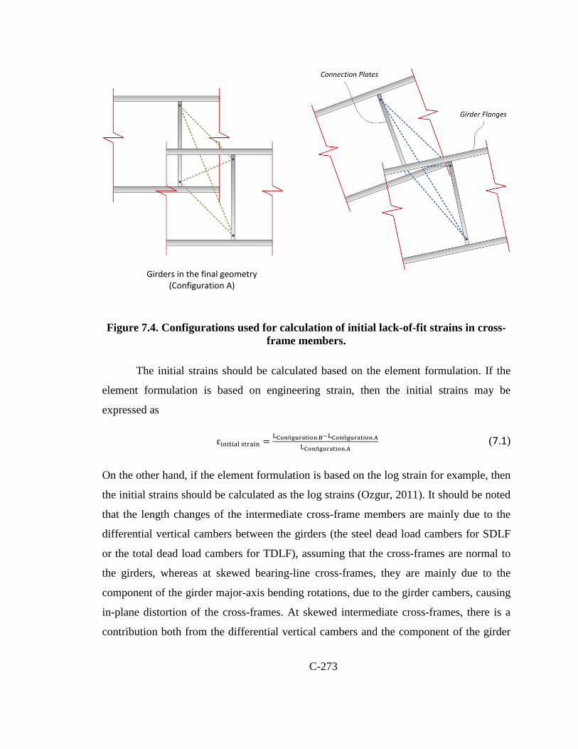
C-273

Figure 7.4. Configurations used for calculation of initial lack-of-fit strains in cross-frame members.

The initial strains should be calculated based on the element formulation. If the

element formulation is based on engineering strain, then the initial strains may be

expressed as

εinitial strain =LCon�iguration.B−LCon�iguration.A

LCon�iguration.A (7.1)

On the other hand, if the element formulation is based on the log strain for example, then

the initial strains should be calculated as the log strains (Ozgur, 2011). It should be noted

that the length changes of the intermediate cross-frame members are mainly due to the

differential vertical cambers between the girders (the steel dead load cambers for SDLF

or the total dead load cambers for TDLF), assuming that the cross-frames are normal to

the girders, whereas at skewed bearing-line cross-frames, they are mainly due to the

component of the girder major-axis bending rotations, due to the girder cambers, causing

in-plane distortion of the cross-frames. At skewed intermediate cross-frames, there is a

contribution both from the differential vertical cambers and the component of the girder

Girders in the final geometry (Configuration A)

Girders “locked” in their initially plumb cambered geometry, cross-frames subjected to initial strains

to connect to the girders (Configuration B)

C-274

major-axis bending rotations (due to the camber) causing in-plane distorton of the cross-

frames.

In 2D-grid analysis models, the cross-frames typically are modeled with single

equivalent beam elements. It is possible to include the initial lack-of-fit effects in the

analysis using the equivalent beam elements presented in Chapter 6 and in Sanchez

(2011), as well as using conventional beam elements. For this purpose, the initial nodal

forces associated with the lack-of-fit between the girders and cross-frames are calculated

by taking the product of the cross-frame equivalent beam element stiffness matrices with

the following equivalent beam element lack-of-fit displacements:

• For intermediate cross-frames that are normal to the girders, the differential total

dead load camber (for TDLF) or the differential steel dead load camber (for

SDLF) (see Figure 7.5).

• For cross-frames on skewed bearing lines, the cross-frame end rotations caused by

the girder total dead load camber rotations (for TDLF) or the steel dead load

camber rotations (for SDLF) (see Figures 7.6 and 7.7).

• For skewed intermediate cross-frames, a combination of the above two effects.

It should be noted that the twisting of the cross-frames has a negligible effect on initial

lack-of-fit forces; therefore, the twisting of the cross-frames can be neglected when

calculating the initial lack-of-fit forces.

Figure 7.5. Imposed differential vertical camber to calculate initial lack-of-fit forces in the plane of an intermediate cross-frame framed normal to the girders.

Equivalent beam element representation of intermediate cross-frame framed normal to the girders.

Differential total dead load camber (for TDLF) orDifferential steel dead load camber (for SDLF)

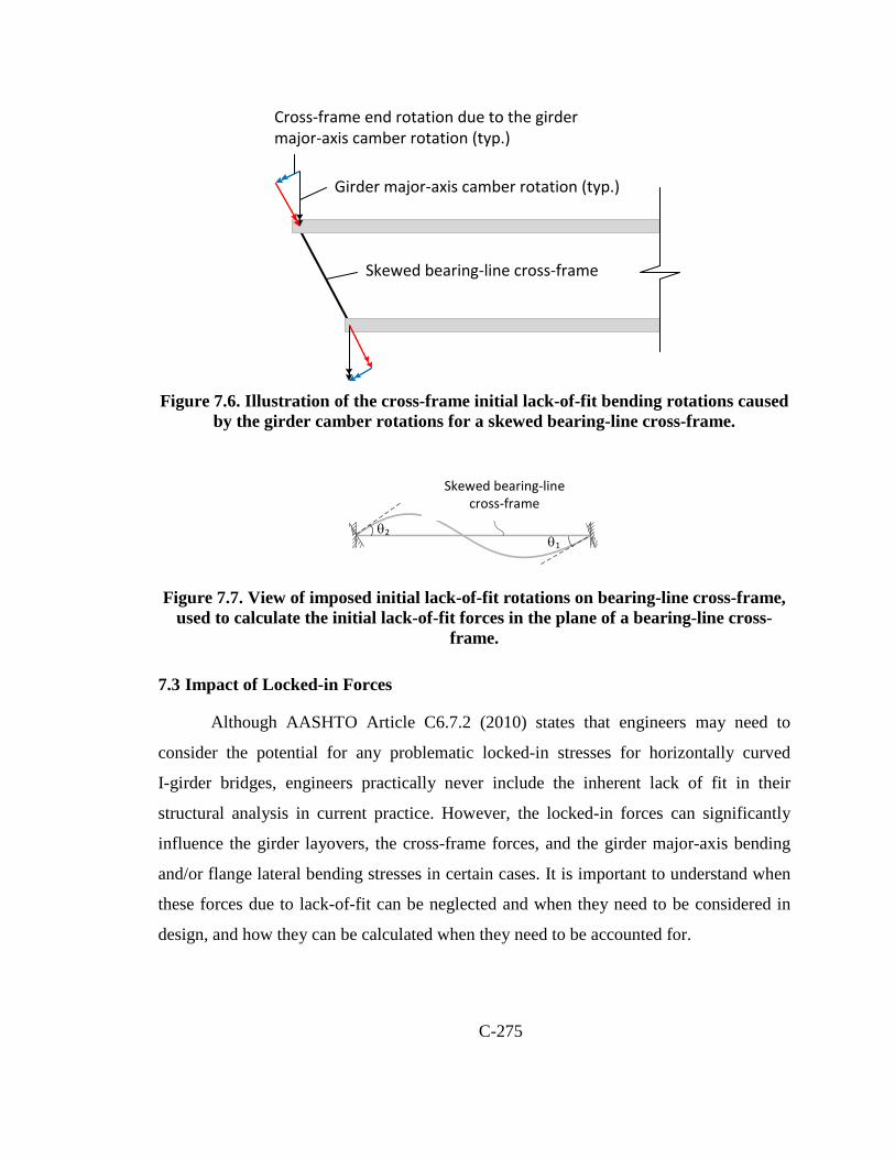
C-275

Figure 7.6. Illustration of the cross-frame initial lack-of-fit bending rotations caused

by the girder camber rotations for a skewed bearing-line cross-frame.

Figure 7.7. View of imposed initial lack-of-fit rotations on bearing-line cross-frame, used to calculate the initial lack-of-fit forces in the plane of a bearing-line cross-

frame.

7.3 Impact of Locked-in Forces

Although AASHTO Article C6.7.2 (2010) states that engineers may need to

consider the potential for any problematic locked-in stresses for horizontally curved

I-girder bridges, engineers practically never include the inherent lack of fit in their

structural analysis in current practice. However, the locked-in forces can significantly

influence the girder layovers, the cross-frame forces, and the girder major-axis bending

and/or flange lateral bending stresses in certain cases. It is important to understand when

these forces due to lack-of-fit can be neglected and when they need to be considered in

design, and how they can be calculated when they need to be accounted for.

Skewed bearing-line cross-frame

Girder major-axis camber rotation (typ.)

Cross-frame end rotation due to the girder major-axis camber rotation (typ.)

Skewed end cross-frame

θ1

θ2

Skewed bearing-line cross-frame

C-276

7.3.1 Girder Layovers

As noted previously, bridge I-girders in curved and/or skewed bridges generally

can be plumb only in one load condition. The cross-frames are relatively stiff within their

planes compared to the torsional stiffness of the I-girders. Therefore, a common

assumption is that the girders can be twisted and forced to fit the cross-frames under any

lack-of-fit. However, twisting of the girders can be difficult in cases where the twist is

coupled significantly with major-axis bending rotations and vertical deflections. This is

often the case for curved girders for example. The ultimate goal with any DLF (Dead

Load Fit, i.e., TDLF or SDLF) detailing is to obtain plumb webs at the targeted load level

by using the rigidity of the cross-frames to impose girder torsional rotations opposite to

the dead load torsional rotations. Within the span, the direction of the torsional rotations

is mainly driven by the differential vertical camber (assuming that the cross-frames are

normal to the girders). At the bearing lines, it is driven mainly by the rotational

compatibility with the bearing line cross-frames and the direction of the girder end

rotations due to the camber. The differential vertical camber between the girders and the

rotational compatibility at the bearing lines associated with the girder camber rotations

are the primary sources of the lack-of-fit for SDLF and TDLF detailing.

Figures 7.8 and 7.9 show a representative set of total dead load girder camber

profiles and the corresponding differential camber between the girders for a straight

I-girder bridge with parallel skew and curved I-girder bridge with radial supports

respectively. In these figures, the sign of the differential camber is positive when the

girder with the larger number has the larger camber. For instance, the differential camber

between girders G2 and G1 at the bottom left corner of the bridge in Figure 7.8(b) is

+3.4, meaning that the camber is 3.4 inches higher in girder G2 at the first intermediate

cross-frame from the bearing line. Conversely, the differential camber between girders

G8 and G9 at the upper right corner of the bridge is -3.4 inches, indicating that the

camber in G8 is 3.4 inches higher than in G9 at the first intermediate cross-frame. The

differential camber between the girders can be either positive or negative depending on

the difference between the girder camber profiles at the cross-frame locations, as

illustrated in Figure 7.10.

C-277

(a) Girder cambers under total dead load

(b) Differential camber between the girders

Figure 7.8. NISSS54, Girder cambers and the differential camber between the girders obtained from FEA vertical deflections.

0

2

4

6

8

10

12

14

16

18

0 50 100 150 200 250 300 350 400 450 500

Gird

er C

ambe

rs (i

n.)

Girder Length (ft)

G1 G2 G3 G4 G5 G6 G7 G8 G9

G1

G9

z (ft)

z = 0

z = 505'

z = 302'

z = 203'

z (ft)

0.92.13.40.0

1.22.02.80.0

0.81.52.22.63.10.0

0.81.52.12.63.00.0

0.00.81.52.12.73.13.40.0

0.10.91.72.32.93.33.73.80.0

-0.30.61.42.12.73.23.63.94.10.0

0.21.01.82.43.03.43.84.14.34.40.0

0.0-4.4-4.2-4.0-3.7-3.4-2.9-2.4-1.7-1.0-0.1

0.00.0

0.00.0

0.00.0

0.0

-4.1-3.9-3.6-3.2-2.7-2.1-1.4-0.60.3-3.8-3.6-3.3-2.8-2.3-1.6-0.80.0

-3.4-3.1-2.7-2.1-1.4-0.70.0-3.0-2.6-2.1-1.5-0.8

-3.1-2.6-2.2-1.5-0.8

-2.8-2.0-1.2-3.4-2.0-0.8

G1

G9Z (ft)

C-278

(a) Girder cambers under total dead load

(b) Differential camber between the girders

Figure 7.9. NISCR2, Girder cambers and the differential camber between the girders obtained from FEA vertical deflections.

0

1

2

3

4

5

6

7

8

0.0 0.2 0.4 0.6 0.8 1.0

Gird

er C

ambe

rs (i

n.)

Normalized Length

G1 G2 G3 G4

G1

G4

0.0

0.0

0.0

0.0

0.0

0.0

-0.8

-0.8

-0.8

-0.8

-0.8

-0.8

-1.4

-1.4

-1.4-1.4

-1.4

-1.4

-1.7-1.7

-1.7-1.7

-1.7-1.7

G1

G4

C-279

(a) Positive differential camber

between the girders

(b) Negative differential camber

between the girders

Figure 7.10. Representative sketch of positive and negative differential camber between the girders (geometric factors such as cross-slope, super-elevation and

profile grade line are not shown for clarity).

For DLF (Dead Load Fit, i.e., TDLF or SDLF) detailing of the intermediate cross-

frames, the girders need to be twisted to connect the cross-frames between them. The

movements at the intermediate cross-frames are illustrated in Figure 7.11 for locations

with positive and negative differential camber between the girders in the no-load geome-

try. In the case of straight bridges with parallel skew orientations, both positive and nega-

tive differential camber are obtained between the girders since the parallel skew orienta-

tion of the bearing lines offsets the camber profiles of the girders as shown in Figure

7.8(a). For instance, the camber profiles for the fascia girders G1 and G9 are the same;

however, the left-hand bearing location for G1 is located at a z coordinate of 203 ft., i.e.,

G1 starts at 203 ft. into the span of G9. The opposite sign of the differential cambers at

each end of the bridge results in a twisting of the girders, due to the lack of fit of the

cross-frames, that is in opposite directions at the two ends. These lack-of-fit twist rota-

tions are in turn opposite in sign relative to the twist rotations of the girders under dead

load.

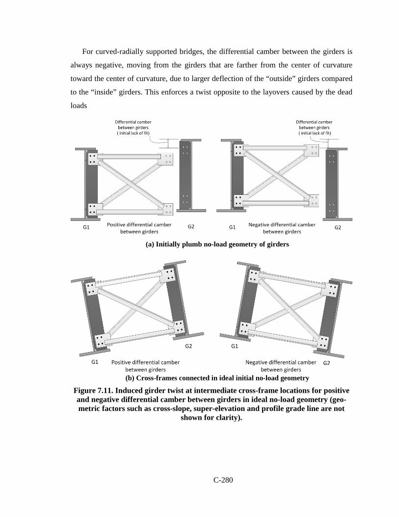
C-280

For curved-radially supported bridges, the differential camber between the girders is

always negative, moving from the girders that are farther from the center of curvature

toward the center of curvature, due to larger deflection of the “outside” girders compared

to the “inside” girders. This enforces a twist opposite to the layovers caused by the dead

loads

(a) Initially plumb no-load geometry of girders

(b) Cross-frames connected in ideal initial no-load geometry

Figure 7.11. Induced girder twist at intermediate cross-frame locations for positive and negative differential camber between girders in ideal no-load geometry (geo-metric factors such as cross-slope, super-elevation and profile grade line are not

shown for clarity).

C-281

The compensating girder layovers generated by DLF detailing are never exactly

equal and opposite to the dead load layovers. (The term “DLF detailing” is used here and

in the following discussions to indicated either SDLF or TDLF detailing.) This is mainly

because:

• The stress state due to the torsional effects of the dead load cannot possibly be

matched exactly by the cross-frame forces induced by the DLF detailing. The

difference between the girder stress state induced by the locked-in forces and the

girder stress state associated with the dead load torsion causes additional

deformations within the structure.

• The girder camber profiles may have been obtained from an analysis that does not

fully capture the true interactions between the girders associated with the three-

dimensional response of the bridge. Furthermore, the SDLF and TDLF detailing

practice of working just with the differential vertical cambers generally neglects

other torsional interactions between the girders and the rest of the structure that

occur via the cross-frames.

As a result, slight deviations from the plumb configuration are observed generally at the

targeted load conditions. However, (Ozgur, 2011) shows that the layover of the girders at

the targeted load conditions tends to be less than a tolerance of ± D /96, where D is the

web depth, regardless of the bridge type and geometry.

Figures 7.12 and 7.13 illustrate the deflected shape of the representative

straight-skewed bridge from Figure 7.8 (NISSS54) under the steel and total dead loads

respectively. Each of these figures shows the magnified deflections associated with each

of the three main types of cross-frame detailing. Similarly, Figures 7.14 and 7.15

illustrate the magnitudes of the girder layovers of this straight-skewed bridge under the

steel and total dead load respectively for each of the types of cross-frame detailing. The

girder layovers are plotted along the length of bridge starting from the left acute corner.

The NISSS54 bridge has a large skew index (IS = 0.68), indicating that the influence of

skew is large on the response of the structure and on the accuracy of the simplified

methods of analysis. The torsional rotations at the bearings due to the total dead load are

more than 0.04 radians in this structure.

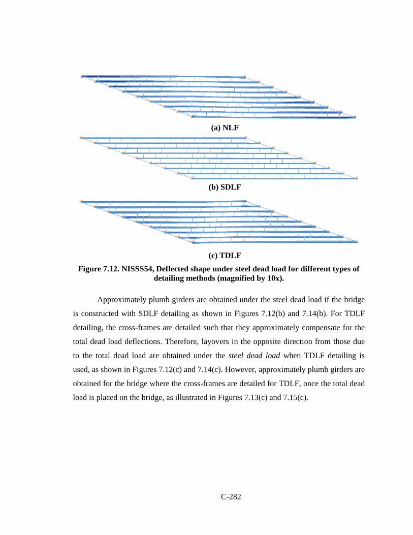
C-282

(a) NLF

(b) SDLF

(c) TDLF

Figure 7.12. NISSS54, Deflected shape under steel dead load for different types of detailing methods (magnified by 10x).

Approximately plumb girders are obtained under the steel dead load if the bridge

is constructed with SDLF detailing as shown in Figures 7.12(b) and 7.14(b). For TDLF

detailing, the cross-frames are detailed such that they approximately compensate for the

total dead load deflections. Therefore, layovers in the opposite direction from those due

to the total dead load are obtained under the steel dead load when TDLF detailing is

used, as shown in Figures 7.12(c) and 7.14(c). However, approximately plumb girders are

obtained for the bridge where the cross-frames are detailed for TDLF, once the total dead

load is placed on the bridge, as illustrated in Figures 7.13(c) and 7.15(c).

C-283

(a) NLF

(b) SDLF

(c) TDLF

Figure 7.13. NISSS54, Deflected shape under total dead load for different types of detailing methods (magnified by 10x).

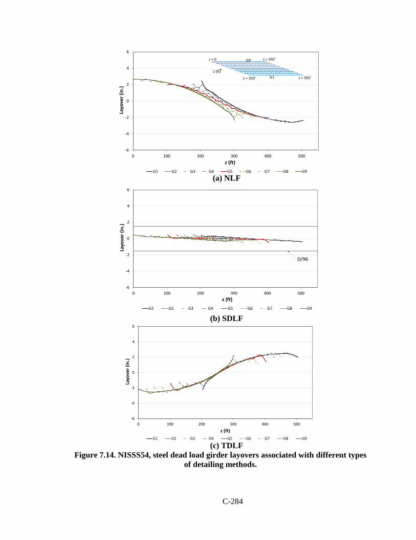
C-284

(a) NLF

(b) SDLF

(c) TDLF

Figure 7.14. NISSS54, steel dead load girder layovers associated with different types of detailing methods.

-6

-4

-2

0

2

4

6

0 100 200 300 400 500

Layo

ver (

in.)

Bridge Length (ft)G1 G2 G3 G4 G5 G6 G7 G8 G9

G1

G9

z (ft)

z = 0

z = 505'

z = 302'

z = 203'

z (ft)

-6

-4

-2

0

2

4

6

0 100 200 300 400 500

Layo

ver (

in.)


D/96

z (ft)

-6

-4

-2

0

2

4

6

0 100 200 300 400 500

Layo

ver (

in.)

z (ft)G1 G2 G3 G4 G5 G6 G7 G8 G9

C-285

(a) NLF

(b) SDLF

(c) TDLF

Figure 7.15. NISSS54, total dead load girder layovers associated with different types of detailing methods.

-6

-4

-2

0

2

4

6

0 100 200 300 400 500

Layo

ver (

in.)


G1

G9

z (ft)

z = 0

z = 505'

z = 302'

z = 203'

z (ft)

-6

-4

-2

0

2

4

6

0 100 200 300 400 500

Layo

ver (

in.)

z (ft)G1 G2 G3 G4 G5 G6 G7 G8 G9

-6

-4

-2

0

2

4

6

0 100 200 300 400 500

Layo

ver (

in.)


D/96

z (ft)

C-286

7.3.2 Cross-Frame Forces

Straight-Skewed I-girder Bridges

In straight-parallel skewed bridges constructed with NLF detailing, relatively

large forces tend to be developed in the cross-frames along the shorter (and stiffer)

diagonal direction between the corners of the structure. Figure 7.16 illustrates this

transverse load path in the NISSS54 bridge by indicating the magnitude of the largest

component force in each of the intermediate cross-frames, normalized by the largest

cross-frame component force. The cross-frames with ratios larger than 0.5, located

between the obtuse corners of the bridge, are highlighted by a different shade.

For straight bridges constructed with TDLF detailing, the locked-in cross-frame

forces are approximately equal and opposite to the total dead load forces in the regions

having the largest transverse stiffness, i.e., in the highlighted region of Figure 7.16.

However, the locked-in forces in the cross-frames tend to be substantially different than

the dead load forces outside of this region.

Large locked-in forces can be developed outside the stiff transverse load paths

depending on the relative lateral stiffness of the adjacent girders and the differential

camber. These “problem” cross-frame locations are typically at intermediate cross-frames

that are at framed too close to the skewed bearing lines.

It should be emphasized that the dead load cross-frame forces from a NLF

analysis are not the opposite of the locked-in forces from a lack-of-fit analysis or

vice-versa. These two sets of forces can be close to being equal and opposite in the

regions of the bridge having the largest transverse stiffness (highlighted in Figure 7.16),

but in other regions, they can be substantially different. This is because stresses and

deformations induced by DLF detailing are not exactly the same as the stresses and

deformations induced by the dead loads.

In the bridge shown in Figure 7.16, the cross-frames in the vicinity of the short

direction between the obtuse corners of the plan tend to have their total dead load forces

mostly relieved by the effects of the TDLF detailing, while the cross-frames in the

C-287

vicinity of the acute corners tend to have their total dead load forces increased relative to

the NLF case. Figures 7.17 and 7.18 show the distribution of the largest total dead load

cross-frame component axial forces in each of the cross-frames throughout the NISSS54

bridge associated with NLF and TDLF detailing cases respectively. The most highly

loaded cross-frame members are highlighted in the darker color, while the more lightly

loaded cross-frame members are shaded light grey. One can observe that the cross-frame

forces along the stiff diagonal direction are significantly reduced by the TDLF detailing,

but they are not zero. In addition, the forces in several of the cross-frame diagonals near

the acute corners are significantly increased.

In straight-skewed bridges constructed with TDLF detailing, cross-frames located

along the stiff transverse load paths may see their largest forces during the steel erection

since the locked-in cross-frame forces are not yet relieved by the dead load forces from

the deck weight. Conversely, straight bridges constructed with SDLF detailing tend to see

the lowest cross-frame forces under the steel dead load.

Curved-Radially Supported I-girder Bridges

The behavior of curved bridges with respect to cross-frame detailing is

significantly different than straight bridges. In curved-radially supported bridges, locked-

in cross-frame forces due to SDLF or TDLF detailing tend to add with the dead load

forces in the cross-frame members, although it should be noted that SDLF detailing

generally results in smaller locked-in forces compared to TDLF detailing. Figures 7.19

and 7.20 illustrate the maximum amplitude of the total dead load component axial forces

in each of the cross-frames for the curved-radially supported bridge considered in Section

7.3.1 (NISCR2). Figure 7.19 shows the results for NLF detailing, whereas Figure 7.20

shows the results for TDLF detailing. The maximum locked-in cross-frame forces occur

in the cross-frames close to the mid-span. This is because the lack-of-fit between the

girders and cross-frames is largest at these locations.

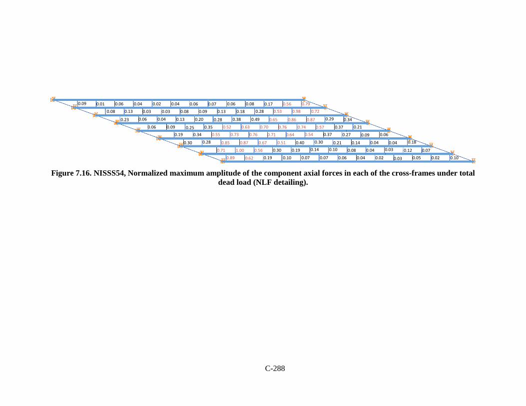
C-288

Figure 7.16. NISSS54, Normalized maximum amplitude of the component axial forces in each of the cross-frames under total

dead load (NLF detailing).

0.190.620.89

0.561.000.71

0.670.870.850.280.30

0.760.730.550.340.19

0.700.630.520.350.250.090.06

0.490.380.280.200.130.040.060.23

0.280.180.130.090.080.030.03

0.09

0.130.08

0.080.060.070.060.040.020.040.060.01

0.100.020.050.030.020.040.060.070.070.10

0.070.120.030.040.080.100.140.190.30

0.180.040.040.140.210.300.400.51

0.060.090.270.370.540.640.71

0.210.370.570.740.76

0.340.290.870.860.65

0.720.980.53

0.790.560.17

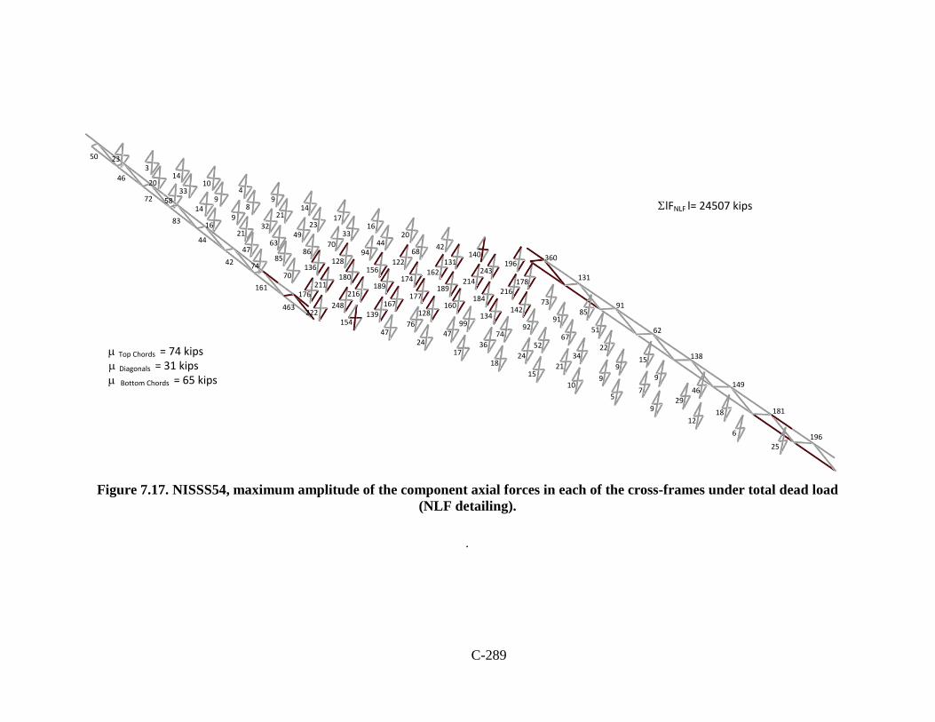
C-289

Figure 7.17. NISSS54, maximum amplitude of the component axial forces in each of the cross-frames under total dead load

(NLF detailing).

.

47154

222463

139248

176161

167216

21170

7442

189180

13685

4744

174156

12886

6321

1683

12294

7049

329

145872

6844

3323

218

933

2046

2016

1714

94

1014

32350

19625

612

95

1015

1817

24

1811829

79

2124

3647

76

14946

99

3452

7499

128

1381522

6792

134160

177

625191

142184

189

9185

73216

214162

131178243

131 360196

14042

ΣlFNLF l= 24507 kips

µ Top Chords = 74 kips

µ Bottom Chords = 65 kips µ Diagonals = 31 kips

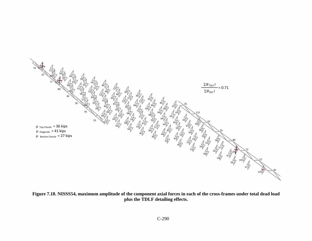
C-290

Figure 7.18. NISSS54, maximum amplitude of the component axial forces in each of the cross-frames under total dead load

plus the TDLF detailing effects.

3436

525568

6344

79

7065

6634

6978

6865

6662

5730

7170

6555

6458

7880

6657

4553

5352

5812577

5137

4448

5155

5472

10467

3030

3746

5459

6056

5713374

81129

57

56

59

58

53

4537

3030

57102

67

55

5451

47

4436

53

72129

57

5252

5245

5767

897855

6355

6470

71

355661

6564

68

5269

3365

6469

1154358

66 3541

3633



ΣlFNLF l

ΣlFTDLF l = 0.71

C-291

Figure 7.19. NISCR2, maximum amplitude of the component axial forces in each of

the cross-frames under total dead load (NLF detailing).

Figure 7.20. NISCR2, maximum amplitude of the component axial forces in each of

the cross-frames under total dead load plus the TDLF detailing effects.

7.3.3 Vertical Displacements

In current practice, the girder camber diagrams are practically always determined

without considering locked-in force effects. However, locked-in forces due to SDLF or

TDLF detailing potentially can have a significant influence on the vertical deflections.

Hence, the physical bridge may exhibit different vertical deflections than assumed in

setting the cambers. This can lead to deviations from the predicted final deck profile and

final girder elevations.


For straight and skewed bridges, the locked-in forces from SDLF or TLDF

detailing tend to have a small effect on the vertical displacements. This is because there is

little to no coupling between the individual girder vertical displacements and the

individual girder twisting for straight I-girders. Figure 7.21 shows total dead load vertical

deflections for the straight-skewed NISSS54 bridge considering each of the types of

cross-frame detailing. It can be observed that there is essentially no difference in the

vertical deflections of the two fascia girders due to the type of cross-frame detailing in

624

4149

4941

243

423

3847

4738

222

312

2024

2420

121

ΣlFNLF l= 1880 kips



430

4756

5647

304

333

5667

6756

323

225

4353

5343

252

ΣlFNLF l

ΣlFTDLF l = 1.40



C-292

this bridge. Both of these girders exhibit approximately 17 inches of vertical deflection at

their mid-span under the total dead load regardless of the method of cross-frame

detailing. The middle girder (Girder 5) has slightly more than 12 inches of vertical

deflection under the total dead load if TDLF detailing is used, whereas it has slightly

more than 11 inches of vertical deflection if NLF detailing is used. These small

differences in the vertical deflections are due to the restraint from the stiff transverse load

path discussed in Section 7.3.2. That is, part of the total dead load tributary to girder G5

is distributed transversely to the bearing lines by the staggered cross-frames framing

between the obtuse corners of the bridge. The development of the forces along this path

causes significant flange lateral bending in girder G5.

The total dead load vertical deflections generally are compensated for by the total

vertical camber in the girders. In current practice, the above differences in the NLF and

TDLF vertical deflections due to the initial lack-of-fit between the girders and cross-

frames are practically never accounted for. One can conclude that the 1 inch difference in

the vertical deflection of Girder 5 is relatively minor. It can be accommodated in the

girder haunch depths when setting the forms for the concrete deck (if the contractor

anticipates the above behavior).

Curved-Radially Supported I-girder Bridges

Conversely, for curved-radially supported bridges, the locked-in forces due to

SDLF or TDLF detailing generally have a significant effect on the vertical displacements

of the girders. This is due to the significant coupling between the major-axis bending and

torsion in curved I-girders. Figure 7.22 shows a representative example from the bridge

NISCR5. The outside girder displacement is reduced by approximately 6 inches due to

the TDLF detailing effects, while the inside girder vertical deflection is reduced by

approximately 4 inches. It should be noted that this bridge is a relatively extreme case

also involving significant global second-order amplification due to the long span and

narrow width of the structure.

C-293

Figure 7.21. NISSS54, Vertical deflections under total dead load associated with

different detailing methods.

-18

-16

-14

-12

-10

-8

-6

-4

-2

0

0.0 0.2 0.4 0.6 0.8 1.0

Vert

ical

Dis

plac

emen

t (in

.)

Normalized Length

GIRDER 1

NLF SDLF TDLF

-18

-16

-14

-12

-10

-8

-6

-4

-2

0

0.0 0.2 0.4 0.6 0.8 1.0

Vert

ical

Dis

plac

emen

t (in

.)

Normalized Length

GIRDER 5

NLF SDLF TDLF

-18

-16

-14

-12

-10

-8

-6

-4

-2

0

0.0 0.2 0.4 0.6 0.8 1.0

Vert

ical

Dis

plac

emen

t (in

.)

Normalized Length

GIRDER 9

NLF SDLF TDLF

G1

G9

Girder G1

Girder G5

Girder G9

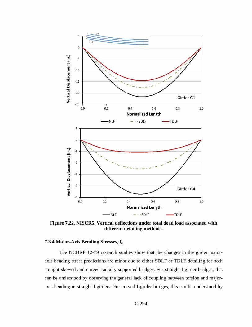
C-294

Figure 7.22. NISCR5, Vertical deflections under total dead load associated with

different detailing methods.

7.3.4 Major-Axis Bending Stresses, fb

The NCHRP 12-79 research studies show that the changes in the girder major-

axis bending stress predictions are minor due to either SDLF or TDLF detailing for both

straight-skewed and curved-radially supported bridges. For straight I-girder bridges, this

can be understood by observing the general lack of coupling between torsion and major-

axis bending in straight I-girders. For curved I-girder bridges, this can be understood by

-25

-20

-15

-10

-5

0

5

0.0 0.2 0.4 0.6 0.8 1.0

Vert

ical

Dis

plac

emen

t (in

.)

Normalized Length

GIRDER 1

NLF SDLF TDLF

-5

-4

-3

-2

-1

0

1

0.0 0.2 0.4 0.6 0.8 1.0

Vert

ical

Dis

plac

emen

t (in

.)

Normalized Length

GIRDER 4

NLF SDLF TDLF

G1

G4

Girder G1

Girder G4

C-295

considering a basic simply-supported curved I-girder with torsionally simply-supported

end conditions subjected to transverse loads as shown in Figure 7.23. The girder torsional

deformations near the end supports have a substantial impact on the mid-span vertical

displacements. However, the girder internal major-axis bending moments and the

corresponding major-axis bending stresses at the mid-span are not affected significantly

by the horizontal curvature.

(a) Undeformed shape

(b) Magnified Deflected shape

Figure 7.23. Illustrative curved girder deformations under dead loads.

7.3.5 Girder Flange Lateral Bending Stresses, f


The girder flange lateral bending stresses under the total dead load are reduced

significantly in straight-skewed bridges due to DLF detailing. If SDLF detailing is used,

the smallest flange lateral bending stresses tend to occur under the steel dead load.

Conversely, if TDLF detailing is used, the smallest flange lateral bending stresses tend to

occur under the total dead load. In these cases the girders largely unwind into their

approximately plumb positions under the corresponding dead load effects.

Engineers sometimes conclude that since the girders were plumb in their no-load

condition, and since they are also plumb in the targeted dead load condition, the girder

flange lateral bending stresses are zero, the cross-frame forces are zero, and the girders

C-296

respond essentially in the manner assumed in a line girder analysis when the bridge is in

the targeted dead load condition. However, it is important to note that the girder flange

lateral bending stresses generally do not completely vanish due to the differences

between the locked-in stresses from the DLF detailing and the stresses related to the

torsion of the girders under the targeted dead load. There are several reasons for this

behavior:

• In particular, local peaks in girder flange lateral bending stresses, as well as cross-

frame forces, can be observed due to “nuisance stiffness effects” at locations such

as intermediate cross-frames that are located too close to skewed bearing lines.

The stresses in the girders due to locked-in force effects do not tend to match the

torsional stresses due to the three-dimensional loading effects in these regions.

• Furthermore, when staggered cross-frames are utilized such as in the NISSS54

bridge, there is substantial flange lateral bending in the interior girders due to the

transverse load transfer effects. The interior girder flanges are loaded “back-and-

forth” in opposing directions by the cross-frames. The corresponding flange

lateral bending in these girders is generally reduced, but it is not completely

nullified by the locked-in force effects.

• Lastly, in the fascia girders, significant flange lateral bending can occur in some

cases due to eccentric overhang bracket loads. These bending effects are of course

not nullified by the locked-in forces from DLF detailing. The NCHRP 12-79

research shows that flange lateral bending stresses in the fascia girders often are

predominantly due to eccentric overhang bracket loads and are not significantly

affected by any of the detailing methods.

In cases with contiguous intermediate cross-frame lines, the total flange lateral bending

stresses associated with DLF detailing are found to be close to zero except in the fascia

girders and at cross-frame locations with nuisance stiffness effects (Ozgur, 2011).

Figure 7.24 shows selected girder major- and minor-axis flange bending stresses

under total dead load for the different types of detailing methods in the NISSS54 bridge.

In this structure, the major-axis bending stresses in the fascia girders are essentially

unaffected by the type of cross-frame detailing. The maximum total dead load flexural

C-297

stress in the top flange of these girders is 30 ksi. The total dead load major-axis bending

stresses in the middle girder (Girder 5) are slightly increased for the TDLF detailing case,

consistent with the larger vertical displacements in Girder 5 for TDLF detailing.

However, the differences in the stresses for the major-axis bending of Girder 5 are

relatively minor. The maximum fb in Girder 5 is approximately 20 ksi under the total

dead load for the TDLF detailing case.

The flange lateral bending stresses are relatively small in the fascia girders for all

the methods of detailing in the NISSS54 bridge, and are predominantly due to eccentric

overhang bracket loads with the exception of the locations near the obtuse corners of the

bridge. At the obtuse corners, relatively large lateral forces are introduced into the fascia

girders from the chords of the first two intermediate cross-frames near the bearing lines.

This causes a “spike” in the flange lateral bending stresses near the ends of the fascia

girders. This spike in f is largest for the NLF detailing case. It is reduced by the locked-in

stresses introduced into the girders in the cases of SDLF and TDLF detailing.

The total dead load lateral bending stresses are significant in Girder 5 regardless

of the method of cross-frame detailing. They are largest for the NLF detailing case,

reaching peak values of nearly 22 ksi near the mid-span. These flange lateral bending

stresses are reduced by the lack-of-fit effects introduced into the girders by SDLF or

TDLF detailing. The resulting maximum total dead load f values are approximately 15

ksi for SDLF detailing and 8 ksi for TDLF detailing. These significant flange lateral

bending stresses in Girder 5 are due to the use of the staggered cross-frames in this bridge

and the “back-and-forth” load transfer effects mentioned previously. Staggered cross-

frames generally are expected to reduce the magnitude of the cross-frame forces that need

to be resisted due to the skew effects, but they introduce “back-and-forth” lateral loads on

the girder flanges in the middle regions of the bridge. These forces are highest near the

mid-span of the middle girders because these locations are in the middle of the stiff

transverse load path first discussed in Section 7.3.2.

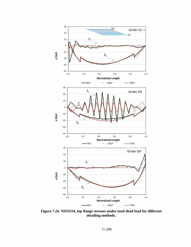
C-298

Figure 7.24. NISSS54, top flange stresses under total dead load for different

detailing methods.

-40

-30

-20

-10

0

10

20

30

0.0 0.2 0.4 0.6 0.8 1.0

σ(k

si)

Normalized Length

GIRDER 1

NLF SDLF TDLF

-40

-30

-20

-10

0

10

20

30

0.0 0.2 0.4 0.6 0.8 1.0

σ(k

si)

Normalized Length

GIRDER 5

NLF SDLF TDLF

-40

-30

-20

-10

0

10

20

30

0.0 0.2 0.4 0.6 0.8 1.0

σ(k

si)

Normalized Length

GIRDER 9

NLF SDLF TDLF

f

fb

f

fb

f

fb

G1

G9

Girder G5

Girder G9

Girder G1

C-299

There is no “spike” in the flange lateral bending stresses in Girder 5 near its ends.

This is because the forces coming into the girder from the intermediate cross-frames near

the support are not as large in Girder 5 as in the exterior fascia girders. The predominant

lateral bending action on Girder 5 is near the middle of the span. Unfortunately, this is

also where the major-axis bending stresses are the highest.

Curved-Radially Supported I-Girder Bridges

For curved-radially supported bridges, the “local” flange lateral bending effects

between the cross-frames due to the horizontal curvature, i.e., the effects associated with

Eq. (2.16), are not influenced by the DLF detailing. However, DLF detailing of curved

bridges induces an overall global lateral bending in the girder flanges in the direction:

• opposite to the overall lateral bending of the girders due to the torsional rotation

of the bridge cross-section,

• opposite to the bending within the girder unbraced lengths between the cross-

frames, and

• in the same direction as the “negative” flange lateral bending stresses due to the

continuity of the curved flanges across the cross-frame locations.

That is, the locked-in forces due to DLF detailing tend to reduce the overall “global”

girder flange lateral bending stresses in curved bridges. Figure 7.25 illustrates this effect

in the NISCR2 bridge. In many curved bridge structures, this overall flange lateral

bending effect is relatively minor. However, in some cases, such as narrow curved bridge

units, this effect can be substantial. These effects are relatively minor in the NISCR2

bridge, although the percentage change in the flange lateral bending stresses on the inside

girder is somewhat large.

C-300

Figure 7.25. NISCR2, Top flange stresses under total dead load for different

detailing methods.

-10

-5

0

5

10

0.0 0.2 0.4 0.6 0.8 1.0

σ(k

si)

Normalized Length

GIRDER 4

NLF SDLF TDLF

-30

-25

-20

-15

-10

-5

0

5

10

0.0 0.2 0.4 0.6 0.8 1.0

σ(k

si)

Normalized Length

GIRDER 1

NLF SDLF TDLF

-20

-15

-10

-5

0

5

10

0.0 0.2 0.4 0.6 0.8 1.0

σ(k

si)

Normalized Length

GIRDER 2

NLF SDLF TDLF

f

fb

f

fb

f

fb

G1

G4

Girder G1

Girder G2

Girder G4

C-301

7.4 Impact of Locked-in Force Effects on Strength

Locked-in force effects tend to be additive with the dead load responses for the

cross-frame forces and the maximum (“negative”) girder flange lateral bending stresses

in curved and radially-supported bridges. The AASHTO LRFD Specifications provide

explicit provisions for checking of strength during construction. Ozgur (2011) observes

that additional locked-in force effects due to DLF detailing do not affect the bridge

system strength significantly assuming that the cross-frames are sized adequately and that

the critical components are the girders. In fact, Ozgur (2011) demonstrates that locked-in

force effects can increase the strength of the curved bridges that are susceptible to overall

second-order effects or significant overall (global) flange lateral bending. One example of

this bridge type is provided in Section 2.9. Unfortunately, DLF detailing of horizontally

curved bridges tends to increase the cross-frame member forces.

Example load-deflection curves from two bridges studied by the NCHRP 12-79

project, NISCR2 and NISCR5, are shown in Figures 7.26 and 7.27 respectively. The

applied load fraction (ALF) is the multiple of the nominal total dead load applied to the

bridge.

NISCR2 is a shorter bridge (150 ft.span) with a 30 ft.deck width that shows

relatively little influence of the type of detailing on the overall bridge capacity. However,

NISCR5 is a more extreme 300 ft.simple-span bridge with a 30 ft.deck width and no

flange-level lateral bracing system. This bridge experiences significant second-order

effects under the total dead load. It is only able to develop 1.34 times the total dead load

before reaching its capacity for the case with NLF detailing. However, with TDLF

detailing, the overall torsional rotations are reduced, thus reducing the second-order

amplification and resulting in a load capacity of 1.54 times the nominal total dead load.

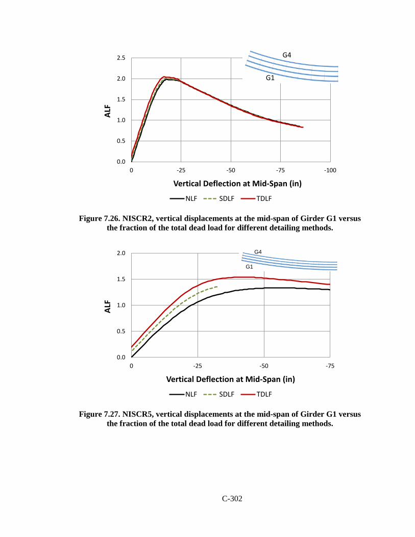
C-302

Figure 7.26. NISCR2, vertical displacements at the mid-span of Girder G1 versus

the fraction of the total dead load for different detailing methods.

Figure 7.27. NISCR5, vertical displacements at the mid-span of Girder G1 versus

the fraction of the total dead load for different detailing methods.

0.0

0.5

1.0

1.5

2.0

2.5

-100-75-50-250

ALF

Vertical Deflection at Mid-Span (in)

NLF SDLF TDLF

G1

G4Girder 1

0.0

0.5

1.0

1.5

2.0

-75-50-250

ALF

Vertical Deflection at Mid-Span (in)

NLF SDLF TDLF

G1

G4

C-303

7.5 Special Cases

7.5.1 Special Cases where a Line Girder Analysis Predicts Accurate Results for Straight-Skewed Bridges

Engineers widely use line-girder analysis solutions to design straight skewed I-girder

bridges. The corresponding analysis predictions impact the responses associated with the

detailing of the cross-frames since the camber profiles are set based on these predictions.

Figure 7.28 shows two sets of total dead load girder camber profiles for the bridge

NISSS54, one based on line-girder analysis and one based on 3D-FEA. The 3D-FEA

solution is conducted assuming NLF detailing, which neglects the small influence of the

SDLF or TDLF cross-frame detailing on the corresponding vertical displacements. It is

obvious that the line-girder analysis solutions are not capable of capturing any

interactions of the individual girders with the NISSS54 bridge system.

In the line-girder analyses, the girders are modeled individually disregarding any

interactions with the other framing. The dead loads applied to the individual girders are

based on their tributary areas, and the interactions between the cross-frames and girders

are neglected. Therefore, the line-girder analyses do not predict any torsion of the girders.

Of course, if the cross-frames are detailed for SDLF or TDLF, and if this detailing works

as intended, then the girders ideally will not be subjected to any torsion under the steel

dead load or the total dead load respectively. Hence, it may be possible that a line-girder

analysis will be sufficient to capture the physical vertical displacements and major-axis

bending stresses with good accuracy for straight skewed bridges, constructed with DLF

detailing, under the load level at which the girder webs are theoretically plumb.

Ozgur (2011) shows that if Total Dead Load Fit (TDLF) detailing is used on straight

skewed I-girder bridges (i.e., the cross-frames are detailed for plumb webs in the final

dead load condition), and if the girder cambers are set based on the results from 1D line-

girder analyses, the locked-in stresses due to the cross-frame detailing come very close to

canceling the stresses due to the torsion of the girders under the total dead load condition.

As such, the physical girder layovers are approximately zero under the total dead load,

and the basic 1D line girder analysis flexural model is sufficient to capture the physical

vertical displacement and major-axis bending stresses with good accuracy. This result is

C-304

essentially independent of the magnitude and pattern of the support skews. Furthermore,

Ozgur (2011) illustrates that the cross-frame forces along the stiff diagonal direction, as

well as the corresponding flange lateral bending stresses, are significantly reduced if the

bridge is constructed with TDLF detailing based on the cambers from line girder analysis.

However, they are not zero. Unfortunately, the line girder analysis does not provide any

predictions for these non-zero flange lateral bending stresses and the cross-frame forces.

(a) Line girder analysis

(b) 3D FEA

Figure 7.28. NISSS54, Girder camber profiles, obtained from different analysis solutions.

0

2

4

6

8

10

12

14

16

18

0 50 100 150 200 250 300 350 400 450 500

Gird

er C

ambe

rs (i

n.)

Girder Length (ft)

G1 G2 G3 G4 G5 G6 G7 G8 G9

G1

G9

z (ft)

z = 0

z = 505'

z = 302'

z = 203'

z (ft)

0

2

4

6

8

10

12

14

16

18

0 50 100 150 200 250 300 350 400 450 500

Gird

er C

ambe

rs (i

n.)

Girder Length (ft)

G1 G2 G3 G4 G5 G6 G7 G8 G9

z (ft)

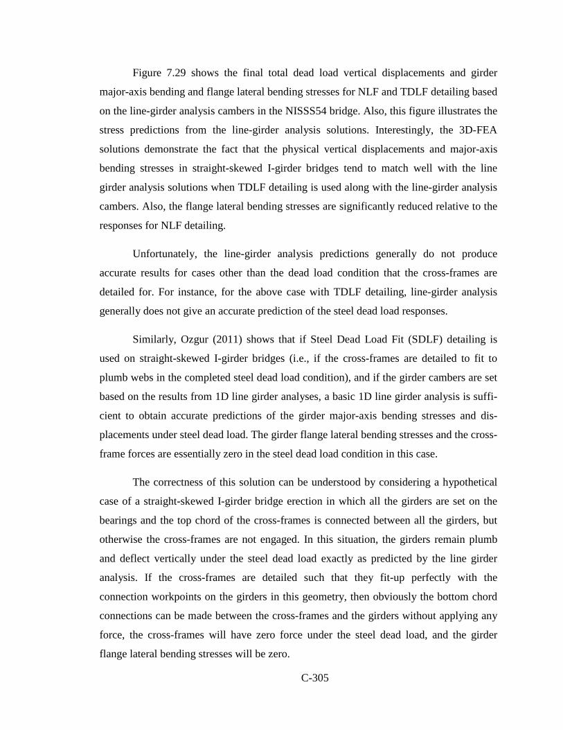
C-305

Figure 7.29 shows the final total dead load vertical displacements and girder

major-axis bending and flange lateral bending stresses for NLF and TDLF detailing based

on the line-girder analysis cambers in the NISSS54 bridge. Also, this figure illustrates the

stress predictions from the line-girder analysis solutions. Interestingly, the 3D-FEA

solutions demonstrate the fact that the physical vertical displacements and major-axis

bending stresses in straight-skewed I-girder bridges tend to match well with the line

girder analysis solutions when TDLF detailing is used along with the line-girder analysis

cambers. Also, the flange lateral bending stresses are significantly reduced relative to the

responses for NLF detailing.

Unfortunately, the line-girder analysis predictions generally do not produce

accurate results for cases other than the dead load condition that the cross-frames are

detailed for. For instance, for the above case with TDLF detailing, line-girder analysis

generally does not give an accurate prediction of the steel dead load responses.

Similarly, Ozgur (2011) shows that if Steel Dead Load Fit (SDLF) detailing is

used on straight-skewed I-girder bridges (i.e., if the cross-frames are detailed to fit to

plumb webs in the completed steel dead load condition), and if the girder cambers are set

based on the results from 1D line girder analyses, a basic 1D line girder analysis is suffi-

cient to obtain accurate predictions of the girder major-axis bending stresses and dis-

placements under steel dead load. The girder flange lateral bending stresses and the cross-

frame forces are essentially zero in the steel dead load condition in this case.

The correctness of this solution can be understood by considering a hypothetical

case of a straight-skewed I-girder bridge erection in which all the girders are set on the

bearings and the top chord of the cross-frames is connected between all the girders, but

otherwise the cross-frames are not engaged. In this situation, the girders remain plumb

and deflect vertically under the steel dead load exactly as predicted by the line girder

analysis. If the cross-frames are detailed such that they fit-up perfectly with the

connection workpoints on the girders in this geometry, then obviously the bottom chord

connections can be made between the cross-frames and the girders without applying any

force, the cross-frames will have zero force under the steel dead load, and the girder

flange lateral bending stresses will be zero.

C-306

(a) Vertical Displacements

(b) Top Flange Stresses

Figure 7.29. NISSS54, total dead load vertical deflections and top flange stresses associated with NLF and TDLF detailing where the cambers are set based on line girder analysis results.

-18

-16

-14

-12

-10

-8

-6

-4

-2

0

0.0 0.1 0.2 0.3 0.4 0.5 0.6 0.7 0.8 0.9 1.0

Vert

ical

Dis

plac

emen

t (in

.)

Normalized Length

GIRDER 1

NLF-FEA TDLF-FEA, LGA Camber NLF-LGA

G1

G9

-18

-16

-14

-12

-10

-8

-6

-4

-2

0

0.0 0.2 0.4 0.6 0.8 1.0

Vert

ical

Dis

plac

emen

t (in

.)

Normalized Length

GIRDER 5


-40

-30

-20

-10

0

10

20

30

0.0 0.2 0.4 0.6 0.8 1.0

σ(k

si)

Normalized Length

GIRDER 1


G1

G9

f

fb

-40

-30

-20

-10

0

10

20

30

0.0 0.2 0.4 0.6 0.8 1.0σ

(ksi

)Normalized Length

GIRDER 5


f

fb

C-307

This solution is achieved via an accurate 2D-grid analysis (satisfying the

recommendations of Chapter 6), or via the above 3D FEA, by including the effect of the

corresponding lack-of-fit between the girders and the cross-frames in the initial no-load

geometry. This lack-of-fit induces cross-frame forces and girder flange lateral bending

stresses that in this ideal case are equal and opposite to the cross-frame forces and girder

flange lateral bending stresses in the three-dimensional structural system under the steel

dead load. Interestingly, if the cambers are obtained as the negative of the vertical

displacements associated with this three-dimensional response (Figure 7.28b), the locked-

in forces will tend to offset the dead-load forces in the cross-frames under the steel dead

load such that the sum of these two effects will be relatively small. However, the

resulting cross-frame forces are not zero, and the corresponding flange lateral bending

stresses are not zero. The cambers determined from the line girder analysis (Figure 7.28a)

are the ones that produce locked-in forces, due to the corresponding initial lack-of-fit,

that perfectly offset the steel dead load cross-frame forces.

7.5.2 Special Cases where Line Girder Analysis with the V-load Approximation Predicts Accurate Results for Curved Radially-Supported Bridges

Line-girder analysis, using the V-load approximation to account for horizontal

curvature effects, is used widely for the analysis and design of curved bridges with radial

supports. In the V-Load analysis, curved girders are modeled as straight girders by using

the girder length along the arc. In addition to dead loads, which are based on the tributary

area of the girders, vertical loads are applied along each span at the connection points of

the cross-frames with girders. The V-load approximations tend to provide good estimates

of the girder stresses and cross-frame forces for simple-span curved radially-supported

bridges. However, variations in flange lateral bending stress predictions can be observed

due to the overall lateral bending of the flanges. Moreover, the vertical displacement

predictions can be off due to the coupling between vertical displacements and torsional

rotations of the girders.

Figure 7.30 shows total dead load girder camber profiles of the NISCR2 bridge,

constructed with NLF detailing based on V-load approximations and 3D-FEA. It can be

C-308

observed from this figure that that the V-load approximations underpredict the vertical

displacements of this bridge.

Ozgur (2011) shows that if Total Dead Load Fit (TDLF) detailing is used on

simply-supported curved I-girder bridges with radial supports (i.e., the bridges are

detailed to have plumb webs in their final dead load condition), and if the girder cambers

are set based on the results from the 1D line-girder analyses with the V-load

approximation, the locked-in stresses due to the cross-frame detailing reduce the overall

(global) flange lateral bending effects. As such, the physical girders are approximately

plumb under total dead load and the flange lateral bending stresses are solely due to

overhang bracket loadings and horizontal curvature effects. That is, the “global” lateral

bending of the flanges due to the overall torsional rotation of the bridge cross-section

(which results in out-of-plumbness of the girder webs along the span) is taken out by the

corresponding locked-in forces. As a result, the basic 1D line-girder analysis flexural

model provides a good representation of the physical vertical displacement and major and

minor axis bending stresses. However, the V-load solutions still do not produce accurate

results for the cross-frame forces, which tend to be increased significantly due to TDLF

detailing. It should be noted that torsional rotation of the bridge cross-section under

general dead load is unavoidable though. Therefore, the V-load analysis does not

necessarily produce accurate results for other dead load conditions in which the webs are

not essentially plumb at the cross-frame locations. In addition, for continuous-span

bridges, other factors enter which can lead to errors in the simplified method. For

instance, the V-load method does not capture the tendency for the vertical reactions at

intermediate supports on the inside of the horizontal curve in a continuous-span bridge to

be somewhat larger due to the transverse load paths provided by the cross-frames.

C-309

(a) Camber based on line girder analysis

(b) Camber based on FEA deflections

Figure 7.30. NISCR2, Total dead load cambers obtained from line girder and finite element analysis solutions.

0

1

2

3

4

5

6

7

8

0.0 0.2 0.4 0.6 0.8 1.0

Gird

er C

ambe

rs (i

n.)

Normalized Length

G1 G2 G3 G4

G1

G4

0

1

2

3

4

5

6

7

8

0.0 0.2 0.4 0.6 0.8 1.0

Gird

er C

ambe

rs (i

n.)

Normalized Length

G1 G2 G3 G4

C-310

Figure 7.31 illustrates the total dead load vertical displacements and girder major-axis

bending and flange lateral bending stresses for NLF and TDLF detailing based on the

cambers from line girder analysis (with V-load adjustments included) in the NISCR2

bridge. Also, Figure 7.31 shows the V-load analysis predictions. The physical vertical

displacements, girder major-axis and flange lateral bending stresses associated with

TDLF detailing are captured accurately by the V-load analysis predictions if the girder

cambers are set based on the V-load analysis solutions.

Similarly, if Steel Dead Load Fit (SDLF) detailing is used on curved I-girder

bridges with radial supports (i.e., the bridges are detailed to have plumb webs in the

completed steel dead load condition) and, if the girder cambers are set based on the

results from 1D line-girder analyses, a basic 1D line-girder analysis (with the V-load

method adjustments) is sufficient to obtain accurate predictions of the girder stresses and

displacements in the steel dead load condition. Unfortunately, in this case, the V-load

analysis generally does not produce accurate results with respect to the physical girder

vertical displacements, major and minor axis bending stresses for other than the steel

dead load condition.

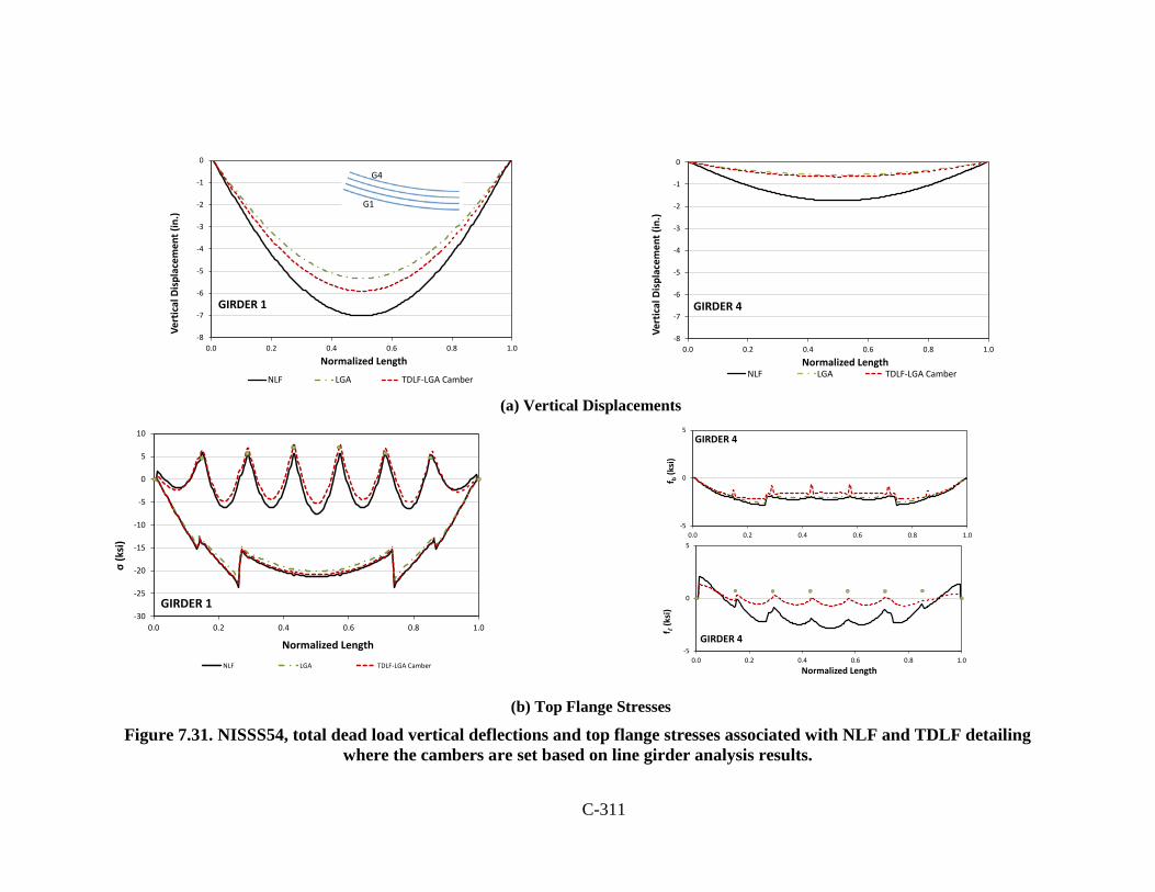
C-311

(a) Vertical Displacements

(b) Top Flange Stresses

Figure 7.31. NISSS54, total dead load vertical deflections and top flange stresses associated with NLF and TDLF detailing where the cambers are set based on line girder analysis results.

-8

-7

-6

-5

-4

-3

-2

-1

0

0.0 0.2 0.4 0.6 0.8 1.0

Vert

ical

Dis

plac

emen

t (in

.)

Normalized Length

GIRDER 1

NLF LGA TDLF-LGA Camber

G1

G4

-8

-7

-6

-5

-4

-3

-2

-1

0

0.0 0.2 0.4 0.6 0.8 1.0

Vert

ical

Dis

plac

emen

t (in

.)

Normalized Length

GIRDER 4


-30

-25

-20

-15

-10

-5

0

5

10

0.0 0.2 0.4 0.6 0.8 1.0

σ(k

si)

Normalized Length

GIRDER 1


-5

0

5

0.0 0.2 0.4 0.6 0.8 1.0

f b(k

si)

Normalized Length

GIRDER 4


-5

0

5

0.0 0.2 0.4 0.6 0.8 1.0f

(ksi

)Normalized Length

GIRDER 4

C-312

7.5.3 Estimating Maximum Dead-Load Fit Cross-Frame Forces and Girder Flange Lateral Bending Stresses Using an Analysis Based on NLF Detailing

In current practice (2012), cross-frame members of straight-skewed bridges are

commonly sized without considering the locked-in forces from SLDF or TDLF detailing

of the cross-frames. However, the physical member-by-member cross-frame forces

corresponding to the sum of the dead load effects plus the locked-in forces from the DLF

detailing can differ substantially from those obtained from an accurate 2D-grid or 3D FE

analysis assuming NLF detailing.

In the previous sections, it is shown that SDLF or TDLF detailing of straight-

skewed bridges tends to develop locked-in cross-frame forces due to the initial lack-of-fit

that are approximately equal and opposite to the dead load stresses in the region having

the largest transverse stiffness, i.e., the shortest diagonal direction across the bridge plan.

However, the locked-in forces in the cross-frames can be substantially different from the

dead load stresses outside this region. Ozgur (2011) shows that the locked-in cross-frame

forces can be relatively large for cross-frames at the vicinity of the skewed bearing lines

outside the short diagonal direction across the bridge plan.

For skewed I-girder bridges, (Ozgur. 2011) provides a minimum ratio of adjacent

unbraced lengths at the first intermediate cross-frame offset from a bearing line such that

large relative lateral stiffness from the adjacent bearing line and large magnitudes of the

differential camber between the girders (and corresponding substantial initial lack-of-fit

vertical displacements) can be alleviated. This ratio is discussed in detail in Chapter 8. If

the minimum ratio of the adjacent unbraced lengths at the first intermediate cross-frame

offset from a bearing line is larger than approximately 0.4, large spikes in the locked-in

cross-frame forces in this cross-frame tend to be eliminated. Furthermore, it is noted that

the maximum cross-frame forces obtained from a 3D FEA assuming NLF detailing are an

accurate to conservative estimate of the maximum cross-frame forces for the physical

bridge using either SDLF or TDLF detailing. Therefore, separate single-size intermediate

and bearing-line cross-frames can be designed conservatively and used throughout the

bridge based on the maximum member forces obtained from an accurate 2D-grid or 3D

C-313

FE analysis neglecting lack-of-fit effects (top chord members designed for the maximum

tension and the maximum compression determined in the top chord at the cross-frames

throughout the bridge, bottom chord members designed similarly, and diagonal members

designed similarly). One cross-frame type can be designed for all the intermediate cross-

frames, and another for the bearing-line cross-frames. In addition, the girder flange lateral

bending stresses tend to be predicted conservatively from an accurate 2D-grid or 3D FE

analysis neglecting lack-of-fit effects given the above caveat.

For curved I-girder bridges, the DLF detailing effects tend to add with the dead

load forces in the cross-frames; therefore, the influence of DLF detailing on the cross-

frame forces, as well as on the girder flange lateral bending stresses at the cross-frames,

generally needs to be included in curved bridges. Fortunately, NLF is often a good option

for curved radially-supported bridges.

For curved and skewed bridges constructed with SDLF or TDLF detailing, the

above effects can go both ways depending on the location within the structure and the

relative magnitudes and directions of the curvature and skew.

Unfortunately, for bridges with larger skew indices, the conservatism of designing

single-size cross-frames in the above fashion can be prohibitive. Since the distribution of

the internal cross-frame forces based on NLF detailing (see Figure 7.17) can be very

different from that obtained based on SDLF or TDLF detailing (see Figure 7.18), the only

alternative if the cross-frames are detailed for SDLF or TDLF is to account for the

corresponding locked-in force effects in the analysis. In addition, note that generally, the

total forces in the steel dead load condition (i.e., the steel dead load forces plus the

locked-in forces) need to be considered. For cases with TDLF detailing, the locked-in

force effects may be significantly larger than the steel dead load effects.

C-314

8. Design and Construction Considerations for Ease of Analysis Via

Improved Behavior

8.1 Limiting the Values of the Bridge Response Indices

The skew effect, torsion, and girder length indices discussed in Chapter 3 can be

used to predict potential difficulties in the early stages of the design of steel girder

bridges. Whenever it is practical, the bridge geometry should be laid out so the indices

are as close to the values of a straight bridge with normal supports, i.e., IS = 0, IT = 0.5,

and IL = 1.0.

Coletti et al. (2010) discuss procedures to reduce the severity of the skew effects

in straight bridges. In all cases, the efforts are aimed at simplifying the structure’s

geometry, which in terms of the proposed indices, is equivalent to reducing the value of

the skew index. As discussed in Section 3.1.2, the possible complications associated to

the skew in both the analysis and the construction of the structure are lessened when IS is

less than 0.30.

Similarly, the torsion index, IT, is a tool that can be used to detect undesired girder

uplift as early as in the preliminary design of a curved and/or skewed bridge (see Section

3.1.4). As discussed in Ozgur (2011), a suggested limit of the torsion index to avoid uplift

under nominal (unfactored) dead plus live load in simple-span I-girder bridges is 0.65. If

IT is above this limit in a given structure, the engineer should anticipate that significant

uplift issues may need to be addressed. Similarly, for simple-span tub-girder bridges with

single bearings on each tub, IT = 0.87 was identified as a limit beyond which bearing

uplift problems are likely. Continuous-span bridges can tolerate larger IT values due to

the continuity with the adjacent spans.

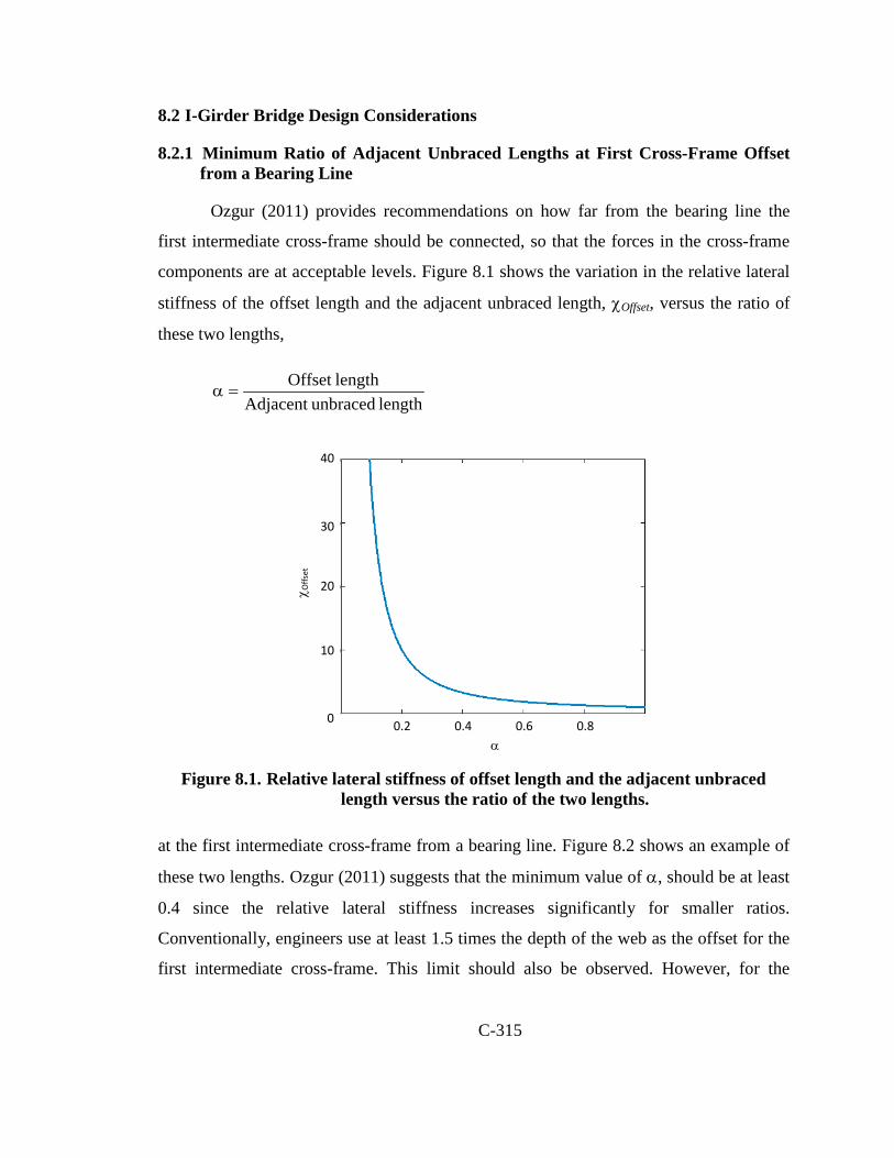
C-315

8.2 I-Girder Bridge Design Considerations

8.2.1 Minimum Ratio of Adjacent Unbraced Lengths at First Cross-Frame Offset from a Bearing Line

Ozgur (2011) provides recommendations on how far from the bearing line the

first intermediate cross-frame should be connected, so that the forces in the cross-frame

components are at acceptable levels. Figure 8.1 shows the variation in the relative lateral

stiffness of the offset length and the adjacent unbraced length, χOffset, versus the ratio of

these two lengths,

length unbracedAdjacent lengthOffset

=α

Figure 8.1. Relative lateral stiffness of offset length and the adjacent unbraced

length versus the ratio of the two lengths.

at the first intermediate cross-frame from a bearing line. Figure 8.2 shows an example of

these two lengths. Ozgur (2011) suggests that the minimum value of α, should be at least

0.4 since the relative lateral stiffness increases significantly for smaller ratios.

Conventionally, engineers use at least 1.5 times the depth of the web as the offset for the

first intermediate cross-frame. This limit should also be observed. However, for the

0

10

20

30

40

0.2 0.4 0.6 0.8

χ Offs

et

α

C-316

bridges with severe skew and long spans, the first intermediate cross-frame should be

offset by a greater length than this conventional distance (i.e., a > 0.4b).

Figure 8.2. Illustration of offset distance and adjacent unbraced length.

8.2.2 Framing of Cross-Frames to Mitigate Skew Effects

The magnitude of the collateral skew effects depends highly on the configuration

of the bracing system. If the cross-frames are laid out so they do not “interfere” with the

rotations that the girders experience at the bearing lines, the flange lateral bending

stresses, and the cross-frame forces are relatively small. Based on this concept, Sanchez

(2011) recommends a scheme that can be implemented in the design of straight I-girder

bridges to mitigate the undesirable effects of skew. The approach is to place the cross-

frames following an orientation similar to the skew. This practice relaxes the large forces

in the cross-frames and the associated girder flange lateral bending stresses that may

result due to skew effects. The basic principle is to connect the girders at the points where

the layovers are similar, so the twists induced by the cross-frames are reduced (Sanchez

(2011) shows that most of the contributions to cross-frame forces and flange lateral

bending come from enforcing layover compatibility). In cases where the skew of the

bearing lines is unequal, the cross-frames can be placed in a “fanned” configuration. With

this layout of the bracing system, the effects of the skew decrease as compared to a

configuration where the cross-frames are connected perpendicular to the girder

longitudinal axis. Figure 8.3 shows an example of this mitigation scheme. The structure

depicted in the figure is Bridge NISSS16. The cross-frame layout shown in Figure 8.3a is

the layout that was considered for the studies of Task 6.

a b

G8

a = offset distance for G8b = adjacent unbraced length for G8

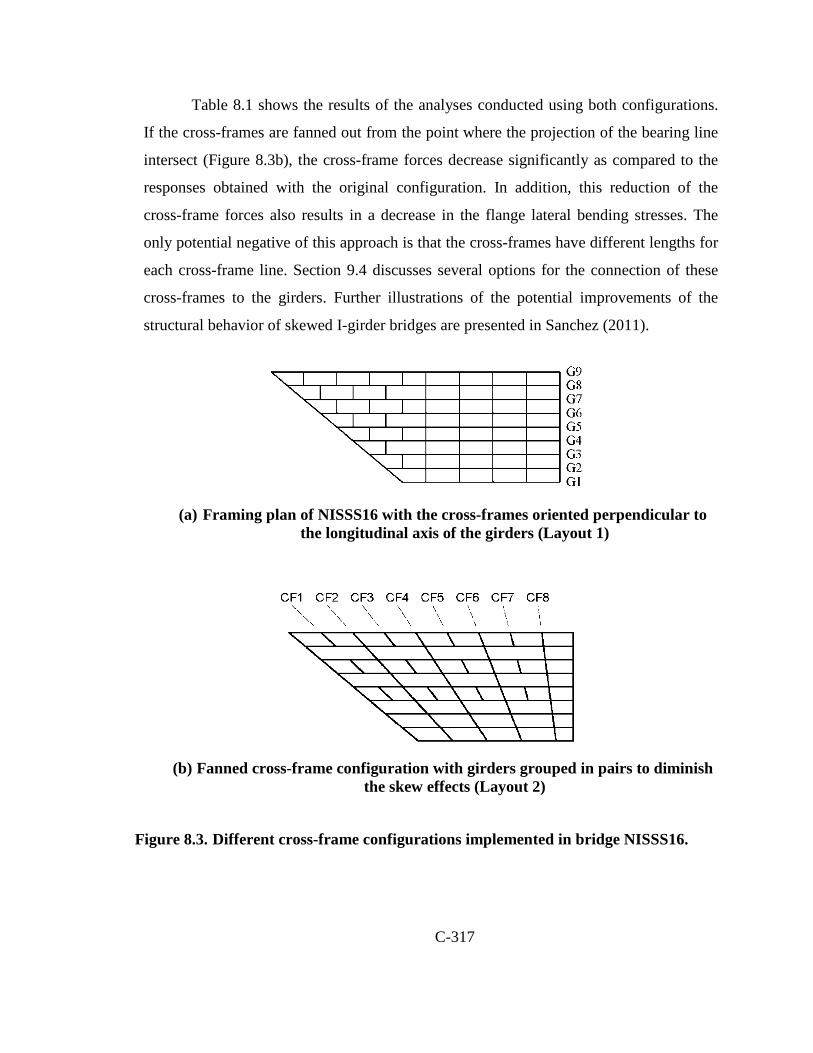
C-317

Table 8.1 shows the results of the analyses conducted using both configurations.

If the cross-frames are fanned out from the point where the projection of the bearing line

intersect (Figure 8.3b), the cross-frame forces decrease significantly as compared to the

responses obtained with the original configuration. In addition, this reduction of the

cross-frame forces also results in a decrease in the flange lateral bending stresses. The

only potential negative of this approach is that the cross-frames have different lengths for

each cross-frame line. Section 9.4 discusses several options for the connection of these

cross-frames to the girders. Further illustrations of the potential improvements of the

structural behavior of skewed I-girder bridges are presented in Sanchez (2011).

(a) Framing plan of NISSS16 with the cross-frames oriented perpendicular to

the longitudinal axis of the girders (Layout 1)

(b) Fanned cross-frame configuration with girders grouped in pairs to diminish

the skew effects (Layout 2)

Figure 8.3. Different cross-frame configurations implemented in bridge NISSS16.

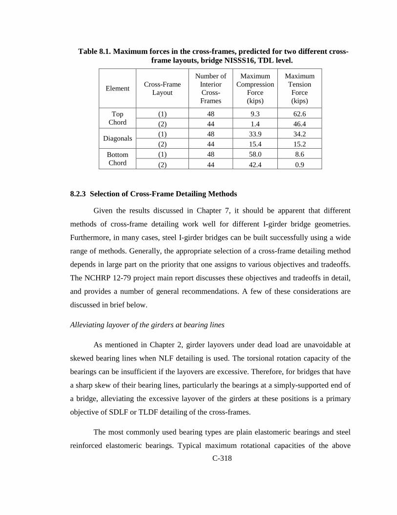
C-318

Table 8.1. Maximum forces in the cross-frames, predicted for two different cross-frame layouts, bridge NISSS16, TDL level.

Element Cross-Frame Layout

Number of Interior Cross-Frames

Maximum Compression

Force (kips)

Maximum Tension Force (kips)

Top Chord

(1) 48 9.3 62.6 (2) 44 1.4 46.4

Diagonals (1) 48 33.9 34.2 (2) 44 15.4 15.2

Bottom Chord

(1) 48 58.0 8.6 (2) 44 42.4 0.9

8.2.3 Selection of Cross-Frame Detailing Methods

Given the results discussed in Chapter 7, it should be apparent that different

methods of cross-frame detailing work well for different I-girder bridge geometries.

Furthermore, in many cases, steel I-girder bridges can be built successfully using a wide

range of methods. Generally, the appropriate selection of a cross-frame detailing method

depends in large part on the priority that one assigns to various objectives and tradeoffs.

The NCHRP 12-79 project main report discusses these objectives and tradeoffs in detail,

and provides a number of general recommendations. A few of these considerations are

discussed in brief below.

Alleviating layover of the girders at bearing lines

As mentioned in Chapter 2, girder layovers under dead load are unavoidable at

skewed bearing lines when NLF detailing is used. The torsional rotation capacity of the

bearings can be insufficient if the layovers are excessive. Therefore, for bridges that have

a sharp skew of their bearing lines, particularly the bearings at a simply-supported end of

a bridge, alleviating the excessive layover of the girders at these positions is a primary

objective of SDLF or TLDF detailing of the cross-frames.

The most commonly used bearing types are plain elastomeric bearings and steel

reinforced elastomeric bearings. Typical maximum rotational capacities of the above

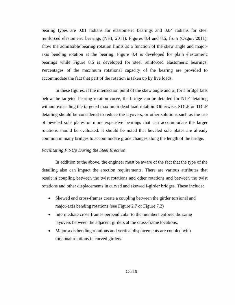
C-319

bearing types are 0.01 radians for elastomeric bearings and 0.04 radians for steel

reinforced elastomeric bearings (NHI, 2011). Figures 8.4 and 8.5, from (Ozgur, 2011),

show the admissible bearing rotation limits as a function of the skew angle and major-

axis bending rotation at the bearing. Figure 8.4 is developed for plain elastomeric

bearings while Figure 8.5 is developed for steel reinforced elastomeric bearings.

Percentages of the maximum rotational capacity of the bearing are provided to

accommodate the fact that part of the rotation is taken up by live loads.

In these figures, if the intersection point of the skew angle and φx for a bridge falls

below the targeted bearing rotation curve, the bridge can be detailed for NLF detailing

without exceeding the targeted maximum dead load rotation. Otherwise, SDLF or TDLF

detailing should be considered to reduce the layovers, or other solutions such as the use

of beveled sole plates or more expensive bearings that can accommodate the larger

rotations should be evaluated. It should be noted that beveled sole plates are already

common in many bridges to accommodate grade changes along the length of the bridge.

Facilitating Fit-Up During the Steel Erection

In addition to the above, the engineer must be aware of the fact that the type of the

detailing also can impact the erection requirements. There are various attributes that

result in coupling between the twist rotations and other rotations and between the twist

rotations and other displacements in curved and skewed I-girder bridges. These include:

• Skewed end cross-frames create a coupling between the girder torsional and

major-axis bending rotations (see Figure 2.7 or Figure 7.2)

• Intermediate cross-frames perpendicular to the members enforce the same

layovers between the adjacent girders at the cross-frame locations.

• Major-axis bending rotations and vertical displacements are coupled with

torsional rotations in curved girders.

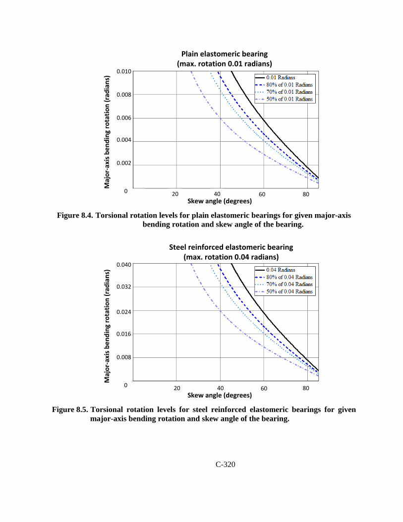
C-320

Figure 8.4. Torsional rotation levels for plain elastomeric bearings for given major-axis

bending rotation and skew angle of the bearing.

Figure 8.5. Torsional rotation levels for steel reinforced elastomeric bearings for given

major-axis bending rotation and skew angle of the bearing.

0.002

0.004

0.006

0.008

0.010

0 20 40 60 80

Maj

or-a

xis b

endi

ng ro

tatio

n (r

adia

ns)

Skew angle (degrees)

Plain elastomeric bearing (max. rotation 0.01 radians)

0.008

0.016

0.024

0.032

0.040

0 20 40 60 80

Maj

or-a

xis b

endi

ng ro

tatio

n (r

adia

ns)

Skew angle (degrees)

Steel reinforced elastomeric bearing (max. rotation 0.04 radians)

C-321

For bridges constructed with NLF detailing, any variation from the no-load geometry due

to dead load deflections requires fit-up forces to assemble the cross-frames in bridges

constructed with NLF. In addition, for bridges constructed with TDLF detailing, fit-up

forces are required at any stage due to lack-of-fit between the cross-frames and girders

(since the total dead load is not yet in place on the girders at the time of the steel

erection). In either case, large fit-up forces can be required if the girders need to be

displaced vertically since the girders generally have large stiffness against major-axis

bending deformations. These cases are more likely to occur at the locations with large

differential vertical displacements between the girders, close spacing between cross-

frames, and deformations for each of the above “coupled interactions” that unfortunately

can be somewhat different from one another. One key location where these factors are

combined is at intermediate cross-frames that are framed close to skewed bearing lines).

SDLF detailing often reduces the incompatibilities between the cross-frames and the

girders close to sharply-skewed bearing lines.

It should be noted that the forces required to assemble the structure during the

erection can depend significantly on the erection procedures. The selected erection

procedure can have a considerable effect on the dead load deflections during erection. For

instance using temporary supports for bridges constructed with NLF detailing or using

the dead load deflections during the erection for bridges constructed with DLF detailing

can reduce any potential large differential vertical displacements. Therefore, fit-up forces

can be reduced based on the selected erection scheme. All these attributes need to be

considered when selecting a particular detailing method.

General Considerations

For straight-skewed bridges, SDLF or TDLF detailing are effective ways to

control the plumbness of the girders, but the minimum ratio of the offset length to the

adjacent unbraced length at the first cross-frame from a bearing line should be taken to be

at least 0.4 to avoid large locked-in cross-frame forces. TDLF detailing is typically a

good option (or the cross-frames can be detailed for an intermediate condition between

TDLF and SDLF) for cases where SDLF detailing does not limit the bearing rotations to

C-322

less than the admissible bearing rotation capacity. It should be noted that in straight-

skewed bridges the fit-up forces tend to be minimal for SDLF detailing and reduced

significantly for TDLF detailing if the steel dead load deflections are used during the

erection of the steel.

For curved-radially supported bridges, NLF detailing is generally an effective

approach since the locked in stresses due to SDLF and TDLF detailing are additive with

the dead load stresses. The fact that the cross-frame forces tend to be smallest with NLF

detailing of these types of bridges (in any dead load condition) is also an indicator that

the fit-up of the steel during the steel erection is easier with NLF detailing. The effect of

the resulting girder layovers on the strength tends to be small (less than approximately 3

%). For cases with three or more girders, the true system capacities tend to be larger than

those implied by the AASHTO LRFD strength calculations regardless of the method of

cross-frame detailing (assuming that the system capacity is governed by the strength of

the girders, i.e., the cross-frames have adequate strength). This is because the girders

generally are able to provide some redistribution of forces to other locations in the bridge

after the first girder limit state is reached.

For I-girder bridges with combined curvature and skew, NLF detailing is effective

for the cases where the bearing rotation limits are not exceeded (see Figures 8.4 and 8.5)

as long as fit-up problems near highly-skewed bearing lines are not exacerbated.

Otherwise, SDLF detailing is often a better option for curved and skewed I-girder

bridges. In the case of SDLF detailing of curved and skewed bridges, the engineer should

consider the locked-in vertical displacements and locked-in force effects in the design.

This is because the locked-in force effects are largely additive with the dead load effects

with respect to the cross-frame forces and the girder maximum (“negative”) flange lateral

bending stresses.

C-323

8.3 Tub-Girder Bridge Design Considerations

8.3.1 Avoid Flange Connections of Diaphragms where Practicable

As discussed previously in Section 2.1.5, the external support diaphragms play an

essential role in the torsional behavior of the system in tub-girder bridges. Also it has

been discussed that the behavior of the diaphragms is based mainly on their in-plane

stiffness while their out-of-plane response is relatively small compared to the system

stiffness.

Previous studies (Helwig et al., 2007) have shown that the flanges of the

diaphragms often do not need to be connected to the tub-girders. The recommended

practice is that the top flange of the diaphragms should not be connected to the top of the

girder as long as the behavior of the diaphragm is dominated by shear. This occurs when

the diaphragm length to depth is less than about 5, a limit that is frequently met by tub-

girder bridge diaphragms. The 3D FEA studies performed for this research agree with the

findings by (Helwig et al., 2007). These recommendations are applicable to full depth

diaphragms only.

8.3.2 Avoid Skewed Intermediate Support Diaphragms

Intermediate support diaphragms connect the tub-girders to distribute the reaction

forces between consecutive girders and restrain the girder cross-section rotations.

However, for continuous span bridges with skewed pier supports, avoiding the external

support diaphragms can be a good design decision. The ETCCS6 (Magruder Blvd

Bridge) shown in Figures 4.44 and 4.45 uses this approach. The plan layout for this

bridge is illustrated in Figure 8.6 where the bearing supports are denoted as crossed

circles. In this figure, it can be observed that the girders are not connected at the skewed

intermediate pier. The omission of the external support diaphragms avoids complex

details at the skewed bearing line, and avoids additional torsional-flexural interactions

from the skew that would have introduced large forces into the bridge. The girders have

sufficient torsional stiffness such that the external support diaphragms may not be

necessary in situations like this. In cases such as this bridge, where there are significant

C-324

span differences between the girders due to the skew, external intermediate cross-frames

or diaphragms perpendicular to the girders within the spans may be useful to control

relative displacements between the girders leading to uneven deck thickness.

Figure 8.6. Plan view of the ETCCS6 bridge (McGruder Boulevard Bridge) showing

intermediate bearing line without external diaphragms.

8.4 Construction Considerations

Forces required to assemble the structure during erection can depend significantly on

the erection procedures (e.g., selection of temporary shoring towers, selection of holding

cranes, etc.) and the sequence of erection, as well as the type of cross-frame detailing,

although the final steel dead load geometry is unique. However, in many cases, the

erection procedures may be driven by the site constraints.

Generally, it is more efficient to erect the girders from the outside of the curve to the

inside of the curve for curved systems. Erecting girders from outside to inside is preferred

since the top flanges of curved girders tend to lay-over in the direction away from the

center of curvature under their dead load. Erecting subsequent girders from the outside

(girders further away from the center of curvature) to the inside (girders closer to the

center of curvature), the self-weight of the components being assembled into the partially

erected structure helps to rotate the previously erected girders back into the desired

geometry. If the girders are erected from inside to outside, large forces may be required

in certain cases to lift the outside girder of the partially erected structure to achieve fit-up

with a new outside girder.

I-girder bridges generally experience 3D deflections during erection, due to torsion,

which can reduce or increase the displacement incompatibilities between connection

points of the structural components. Also, for the given erection stage, displacement

C-325

incompatibilities between connections can be different for different types of cross-frame

detailing.

For NLF detailing, the cross-frames are detailed such that they connect to the

girders in no-load geometry. However, differential displacements between girders can

develop due to dead loads during erection. For I-girder bridges constructed with NLF

detailing, temporary supports (falsework) can be used to control the differential vertical

deflections between adjacent girders by limiting the dead load deflections and stabilizing

the bridge during erection. This is particularly important for I-girder bridges with large

span lengths. Relatively large differential vertical deflections due to dead loads can cause

fit-up problems.

For I-girder bridges with large span-to-width ratios, the girder deflections and

stresses tend to be amplified due to global second-order (stability) effects, as discussed in

Section 2.9. Excessive girder layovers and large differential vertical displacements due to

second-order amplification can lead to fit-up problems or can cause a failure during

erection. However, these problems can be eliminated by the use of temporary supports.

Moreover, significant reduction in the girder stresses and cross-frame forces are observed

for long and narrow I-girder bridge units.

Large differential vertical displacements can be observed between different

parallel bridge units. Figure 8.7 shows a representative bridge NISCS37 where large

differential vertical displacements are observed for a particular erection stage, as shown

in Figure 8.8. Large fit-up forces can be required to connect the different bridge units.

However, temporary supports can reduce the differential vertical displacements between

adjacent girders by limiting the dead load deflections. As a result, fit-up forces required

to connect the cross-frames can be significantly reduced, particularly for bridges

constructed with NLF detailing. Ozgur (2011) shows that that providing temporary

supports across the width of the bridge between the units significantly reduces the large

differential vertical deflections, as illustrated in Figure 8.9 for the bridge NISCS37.

C-326

Steel Dead Load Fit (SDLF) detailing of I-girder bridges tends to minimize the fit-up

forces (and stresses) during the steel erection in straight bridges, unless the bridge is

essentially supported in its no-load condition during the erection. This is because the steel

dead load deflections (and deformations) in the various partially erected units often are

close to the final steel dead load deflections (and deformations). However, in curved

radially-supported bridges, the fit-up forces generally tend to be increased by using SDLF

or TDLF detailing (since the cross-frame forces generally tend to be increased by the

corresponding locked-in forces in these types of bridges).

(i) NISCS37, Possible example of an erection stage.

(ii) NISCS37, Completed steel structure.

Figure 8.7. NISCS37, illustration of long narrow units during construction.

If one provides sufficient temporary supports, holding cranes, etc. such that the

partially erected structure is essentially in a no-load condition, then No-Load Fit (NLF)

detailing minimizes the fit-up forces.

Total Dead Load Fit (TDLF) detailing generally leads to larger fit-up forces since

the steel structure has not yet experienced the concrete dead load, but the cross-frames

are detailed to fit up with the girders once the total dead load cambers are taken out of the

girders.

G1

G4G5

G9

G1

G9

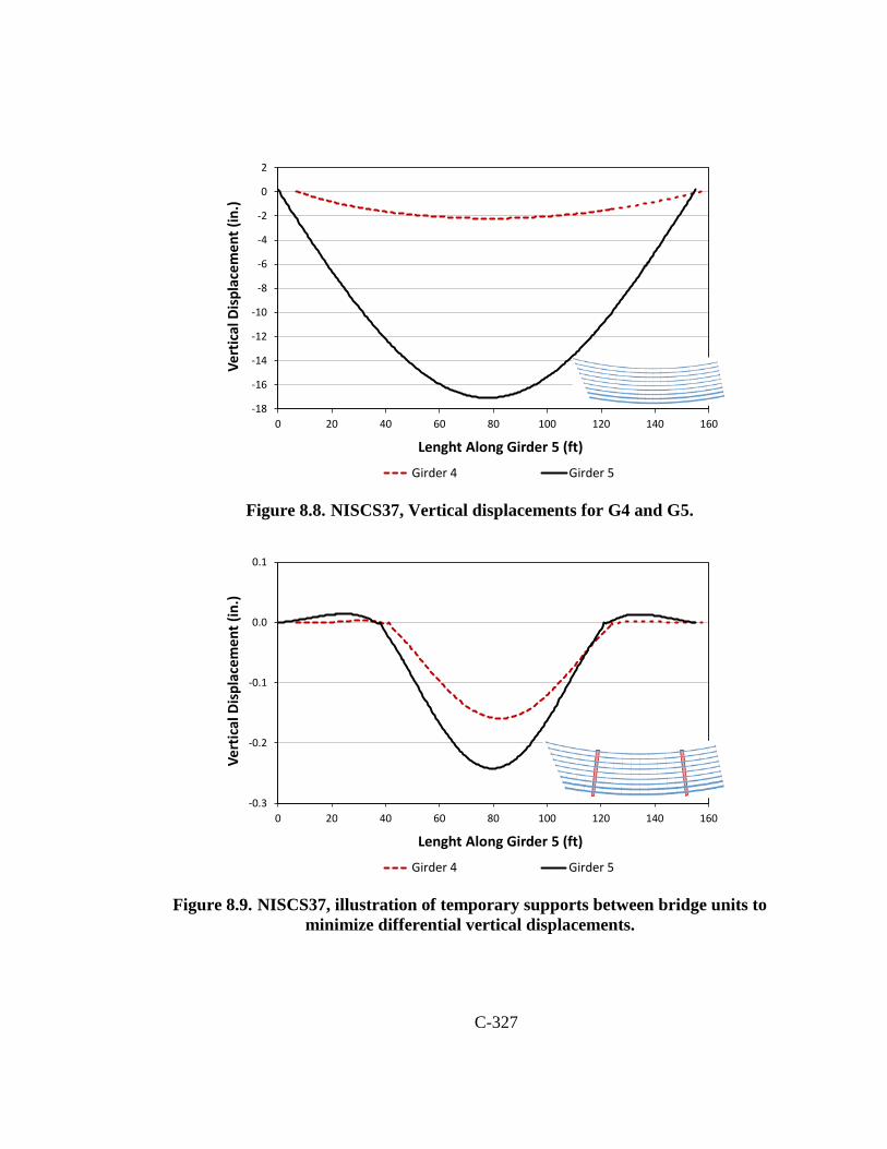
C-327

Figure 8.8. NISCS37, Vertical displacements for G4 and G5.

Figure 8.9. NISCS37, illustration of temporary supports between bridge units to

minimize differential vertical displacements.

-18

-16

-14

-12

-10

-8

-6

-4

-2

0

2

0 20 40 60 80 100 120 140 160

Vert

ical

Dis

plac

emen

t (in

.)

Lenght Along Girder 5 (ft)

Girder 4 Girder 5

-0.3

-0.2

-0.1

0.0

0.1

0 20 40 60 80 100 120 140 160

Vert

ical

Dis

plac

emen

t (in

.)

Lenght Along Girder 5 (ft)

Girder 4 Girder 5

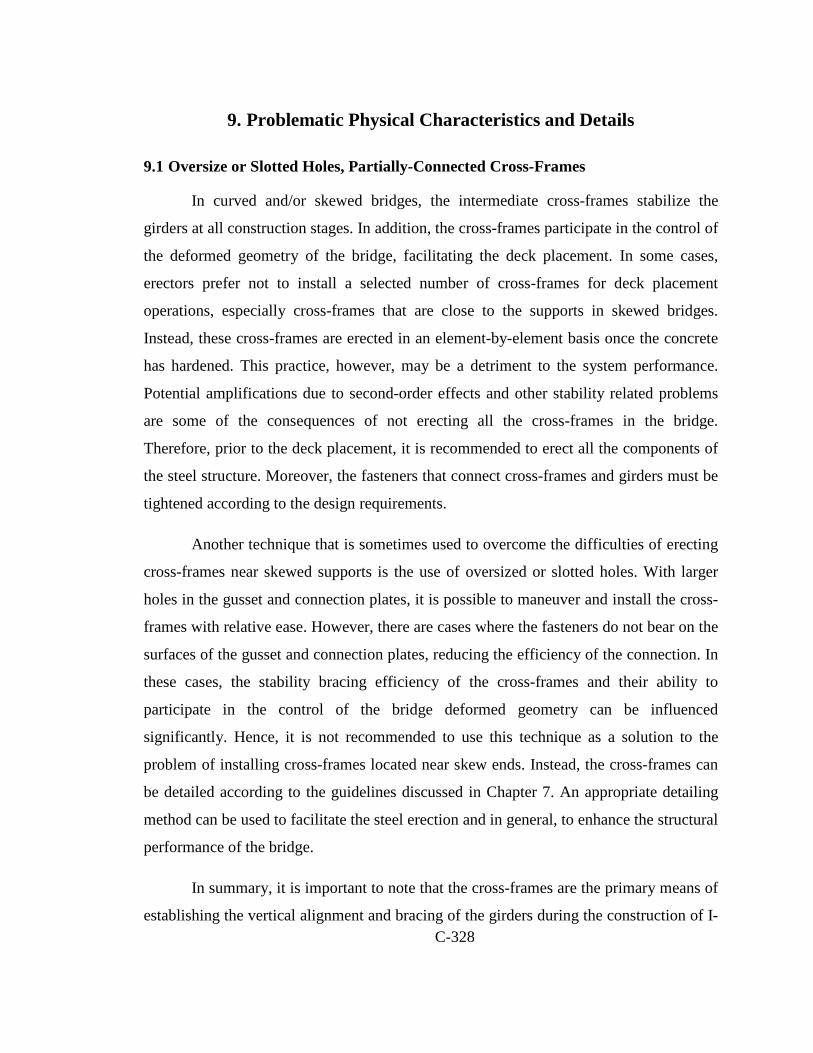
C-328

9. Problematic Physical Characteristics and Details

9.1 Oversize or Slotted Holes, Partially-Connected Cross-Frames

In curved and/or skewed bridges, the intermediate cross-frames stabilize the

girders at all construction stages. In addition, the cross-frames participate in the control of

the deformed geometry of the bridge, facilitating the deck placement. In some cases,

erectors prefer not to install a selected number of cross-frames for deck placement

operations, especially cross-frames that are close to the supports in skewed bridges.

Instead, these cross-frames are erected in an element-by-element basis once the concrete

has hardened. This practice, however, may be a detriment to the system performance.

Potential amplifications due to second-order effects and other stability related problems

are some of the consequences of not erecting all the cross-frames in the bridge.

Therefore, prior to the deck placement, it is recommended to erect all the components of

the steel structure. Moreover, the fasteners that connect cross-frames and girders must be

tightened according to the design requirements.

Another technique that is sometimes used to overcome the difficulties of erecting

cross-frames near skewed supports is the use of oversized or slotted holes. With larger

holes in the gusset and connection plates, it is possible to maneuver and install the cross-

frames with relative ease. However, there are cases where the fasteners do not bear on the

surfaces of the gusset and connection plates, reducing the efficiency of the connection. In

these cases, the stability bracing efficiency of the cross-frames and their ability to

participate in the control of the bridge deformed geometry can be influenced

significantly. Hence, it is not recommended to use this technique as a solution to the

problem of installing cross-frames located near skew ends. Instead, the cross-frames can

be detailed according to the guidelines discussed in Chapter 7. An appropriate detailing

method can be used to facilitate the steel erection and in general, to enhance the structural

performance of the bridge.

In summary, it is important to note that the cross-frames are the primary means of

establishing the vertical alignment and bracing of the girders during the construction of I-

C-329

girder bridges. Leaving out a cross-frame, or providing oversize or slotted holes and

leaving the connections loose amounts to removal of a brace and release of some control

of the geometry.

9.2 Narrow Bridge Units

Under certain circumstances, I-girder bridges can be susceptible to large response

amplifications due to global second-order effects. Contrary to local stability related

problems that involve individual unbraced lengths (see Section 9.3), structures with

relatively large spans-to-width ratios are sensitive to global nonlinear behavior. As

discussed in Section 2.9, these structures may experience excessive displacements that

can compromise the bridge constructability and in some cases, its structural integrity.

Some examples of structures with these characteristics are: widening projects of existing

bridges, pedestrian bridges with twin girders, phased construction, and erection stages

where only a few girders of the bridge are in place.

When the bridge strength is a concern, the equations proposed by Yura et al.

(2008) can be applied to estimate the system buckling load of I-girder bridges. These

equations give a simple approximation of the theoretical load level at which a perfectly

straight system will bifurcate into its buckled configuration. However, the physical bridge

may experience excessive amplification of its lateral-torsional displacements associated

with horizontal curvature, skew, unbalanced construction loads, and dissimilar girders

long before reaching the theoretical buckling load level.

The amplification factor, AFG, can be used to anticipate possible large second-

order amplifications of girder stresses and displacements on a long-and-narrow bridge

unit. To improve the structural performance, it is desirable to limit the value of AFG to

less than approximately 1.25 under the total dead load. If this index is above this limit,

there is a potential for the structure to experience undesired deflections that may affect

the construction process; specifically, the concrete deck placement. It is important to

point out that bridges with AFG ≥ 1.25 do not necessarily need to be redesigned to avoid

global second-order amplification. The construction process can be modified to reduce

this index. For example, the use of temporary shoring towers at mid-span represents a

C-330

significant reduction of AFG. However, it is best for this level of second-order

amplification to be avoided by appropriate consideration at the design stage whenever

possible.

If a bridge has a sufficient number of girders, so that its width is comparable to its

span length, global second order amplifications may be negligible. A decision based on

engineering judgment is required to assess when a bridge structure is vulnerable to global

second-order amplification. The factor AFG is the means to quantify this behavior.

9.3 V-Type Cross-Frames without Top Chords

Cross-frames stabilize the I-girders prior deck hardening. In some cases, V-type

cross-frames without top chords may not be able to perform this function. The flexural

stiffness of this type of cross-frame is substantially smaller than in any other

configuration; therefore, its ability to provide stability bracing needs to be scrutinized

during design. Studies conducted in an existing structure that used this cross-frame

configuration, illustrate the importance of including the top chord. Figure 9.1 shows the

plan view of a bridge located in SR1003 (Chicken Road) bridge over US 74, Robeson

Co., NC. This bridge was instrumented to monitor its behavior during construction. The

field measurements and corresponding original analytical studies are documented in

Morera and Sumner (2009).

L = 133 ft./ w= 30.1 ft./ θ1 = 46.2⁰, θ2 = 46.2⁰

Figure 9.1. EISCS3 bridge layout.

To investigate the influence of the missing top chord on the structural behavior of

this bridge, two cross-frame models are considered in the NCHRP 12-79 research. In the

first analysis, the bridge is modeled to represent the as-built condition, without

C-331

intermediate cross-frame top chords. In the second analysis, the top chords are included.

Figure 9.2 shows a 3D view of both models.

Figure 9.2. Intermediate cross-frame configurations implemented in the analyses.

As observed in the stress and layover plots for the fascia girder, G1, in Figure 9.3,

the flange lateral bending response is affected substantially by the presence of the top

chord. The results from the analysis conducted with the first configuration show that

large lateral displacements may occur in this girder due to the lack of bracing of the top

flange. Similarly, the levels of flange lateral bending stress are very high in the segment

between 0.4 and 0.7 of the girder length. These two responses indicate that if the

incidental contributions from components such as stay-in-place forms, ties between the

girders provided by the contractor, and other devices provided to facilitate the concrete

placement are not considered, the bridge exhibits substantial second order amplifications,

at the TDL level. Sanchez (2011) shows that when the steel structure is properly braced,

the influence of the SIP forms on the system responses during the concrete placement is

negligible.

Configuration 2

Configuration 1

C-332

Figure 9.3. Comparison of stresses and relative lateral displacements for EISCS3 with and without a top chord in the cross-frames (Analysis 1 does not have a top

chord whereas Analysis 2 has a top chord).

9.4 Connections at Skewed Cross-Frame Locations

Bracing systems have a fundamental role on the behavior of curved and skewed I-

girder bridges during construction. In steel bridges, cross-frames are provided to integrate

the structure, transforming the individual girders into a structural system that can support

larger loads than when the girders work separately. For this purpose, cross-frames must

have enough strength and stiffness so they can properly brace the I-girders when the

structure is subjected to the noncomposite loads (Ziemian, 2010).

-40.00

-35.00

-30.00

-25.00

-20.00

-15.00

-10.00

-5.00

0.00

5.00

10.00

0.0 0.1 0.2 0.3 0.4 0.5 0.6 0.7 0.8 0.9 1.0

fb

f

(ksi)

Normalized Lengthfb-Analysis 1 fl-Analysis 1 fb-Analysis 2 fl-Analysis 2

-2.00

-1.00

0.00

1.00

2.00

3.00

4.00

5.00

0.0 0.1 0.2 0.3 0.4 0.5 0.6 0.7 0.8 0.9 1.0

Gir

der L

ayov

er (i

n.)

Normalized Length

Analysis 1 Analysis 2

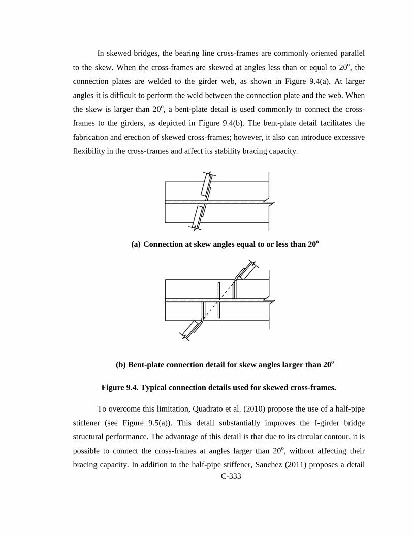
C-333

In skewed bridges, the bearing line cross-frames are commonly oriented parallel

to the skew. When the cross-frames are skewed at angles less than or equal to 20o, the

connection plates are welded to the girder web, as shown in Figure 9.4(a). At larger

angles it is difficult to perform the weld between the connection plate and the web. When

the skew is larger than 20o, a bent-plate detail is used commonly to connect the cross-

frames to the girders, as depicted in Figure 9.4(b). The bent-plate detail facilitates the

fabrication and erection of skewed cross-frames; however, it also can introduce excessive

flexibility in the cross-frames and affect its stability bracing capacity.

(a) Connection at skew angles equal to or less than 20o

(b) Bent-plate connection detail for skew angles larger than 20o

Figure 9.4. Typical connection details used for skewed cross-frames.

To overcome this limitation, Quadrato et al. (2010) propose the use of a half-pipe

stiffener (see Figure 9.5(a)). This detail substantially improves the I-girder bridge

structural performance. The advantage of this detail is that due to its circular contour, it is

possible to connect the cross-frames at angles larger than 20o, without affecting their

bracing capacity. In addition to the half-pipe stiffener, Sanchez (2011) proposes a detail

C-334

that can be implemented to stiffen the bent-plates. As shown in Figure 9.5(b), the bent-

plate can be reinforced to reduce its flexibility by providing stiffeners near the top and

bottom flange. Also, a stiffener at the web mid-depth could be provided to increase the

rigidity of the bent plate.

(a) Half-pipe stiffener (adapted from Quadrato et al. (2010))

(b) Stiffened bent-plate

Figure 9.5. Improved connection details used for skewed cross-frames.

The improved details shown in Figure 9.5 may be used in combination with the

recommendations provided in Section 8.2.2 to mitigate the undesired effects of skew. As

discussed in that section, “fanned” configurations can be used in the design of straight I-

girder bridges, to layout the intermediate cross-frames and reduce the cross-frame forces

and the flange lateral bending stresses.

C-335

9.5 Long-Span I-Girder Bridges without Top Flange Lateral Bracing Systems

In many bridges, the second-order effects are expected to be quite small.

However, second-order amplification due to global flange lateral bending can be large for

individual curved I-girders or for a small number of girders with close spacing relative to

the span length. Additionally, second-order amplification and global flange lateral

bending effects can be more critical for longer spans without flange level lateral bracing

since the stresses are more dominated by dead loads in longer spans. For long-span I-

girder bridges without flange level lateral bracing, the overall bridge system can exhibit

second-order global lateral deflections without significant twisting of the girders.

Figure 9.6 shows the undeflected and deflected geometry (magnified by 20x) of

the bridge NISCR11 under total dead load from the NCHRP project studies. The bridge is

80ft wide and has a 300 ft.span length. However, it does not have a flange-level lateral

bracing system. Figure 9.7 shows the magnitudes of the total dead load deflections of

girder G1 from first- and second-order analyses. Also, Figure 9.8 shows the girder

layovers under total dead load. Although the bridge NISCR11 has nine girders, overall

flange lateral bending of the flanges is observed due to lack of flange-level lateral bracing

system (see Figures 9.9 and 9.10). Figure 9.11 demonstrates the top flange stresses for the

outside girder under total dead load. It should be noted from Figure 9.11 that the girder

flange lateral bending stresses are amplified due to the global flange lateral bending

effects. This example illustrates that as the span length become relatively large, I-girder

bridges without a flange-level lateral bracing system can exhibit significant overall

(global) second-order effects during the deck placement, even when the bridge cross-

section has a relatively large number of girders.

It is suggested from the NCHRP 12-79 studies that I-girder bridges with spans

longer than 200 ft.should be checked for global stability under potential critical stages of

construction unless a flange level lateral bracing system is employed. Flange level lateral

bracing systems are useful to control the geometry since they cause portions of the

structure to act as pseudo-box girders such that large response amplifications due to

global second-order effects can be eliminated.

C-336

(a) Undeflected Geometry

(b) Deflected Geometry

Figure 9.6. NISCR11, undeflected and deflected geometry under total dead load (Magnified by 20x).

Figure 9.7. NISCR11, total dead load vertical displacements from first- and second-

order analyses.

-40

-35

-30

-25

-20

-15

-10

-5

0

5

0.0 0.2 0.4 0.6 0.8 1.0

Vert

ical

Dis

plac

emen

t (in

.)

Normalized LengthG1-Linear G1-Nonlinear

G9-Linear G9-Nonlinear

G1

G9

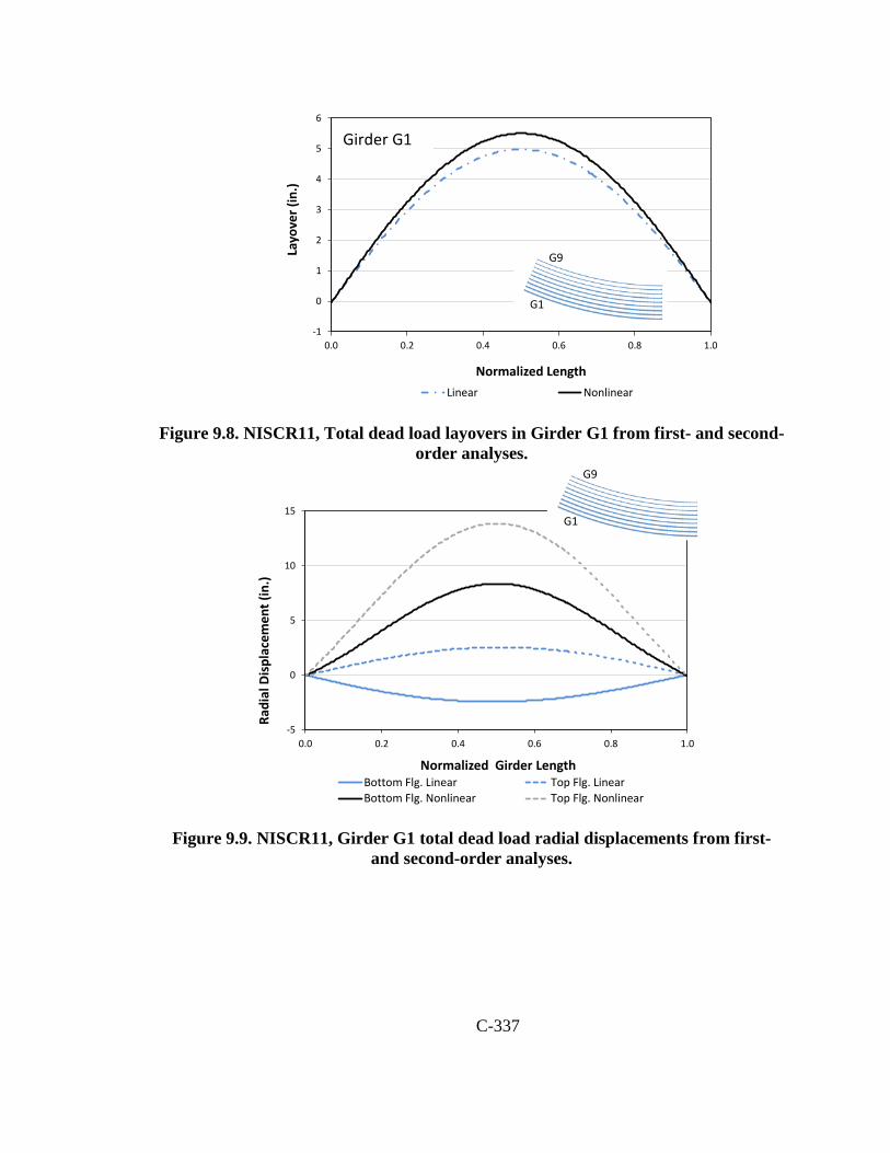
C-337

Figure 9.8. NISCR11, Total dead load layovers in Girder G1 from first- and second-

order analyses.

Figure 9.9. NISCR11, Girder G1 total dead load radial displacements from first- and second-order analyses.

-1

0

1

2

3

4

5

6

0.0 0.2 0.4 0.6 0.8 1.0

Layo

ver (

in.)

Normalized Length

GIRDER 1

Linear Nonlinear

G1

G9

-5

0

5

10

15

0.0 0.2 0.4 0.6 0.8 1.0

Radi

al D

ispl

acem

ent (

in.)

Normalized Girder Length

GIRDER 1

Bottom Flg. Linear Top Flg. LinearBottom Flg. Nonlinear Top Flg. Nonlinear

G1

G9

Girder G1

Girder G1

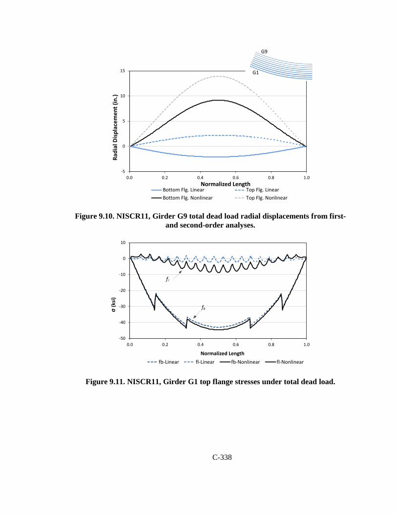
C-338

Figure 9.10. NISCR11, Girder G9 total dead load radial displacements from first- and second-order analyses.

Figure 9.11. NISCR11, Girder G1 top flange stresses under total dead load.

-5

0

5

10

15

0.0 0.2 0.4 0.6 0.8 1.0

Radi

al D

ispl

acem

ent (

in.)

Normalized Length

GIRDER 9

Bottom Flg. Linear Top Flg. LinearBottom Flg. Nonlinear Top Flg. Nonlinear

G1

G9

-50

-40

-30

-20

-10

0

10

0.0 0.2 0.4 0.6 0.8 1.0

σ(k

si)

Normalized Lengthfb-Linear fl-Linear fb-Nonlinear fl-Nonlinear

fb

f

Girder G9

C-339

9.6 Partial Depth End Diaphragms (Tub-Girder Bridges)

Partial depth end diaphragms have been used in some of the existing bridges

collected but not selected for the analytical studies in NCHRP 12-79. This type of detail

should be avoided because it changes the local and global behavior (Helwig et al., 2007).

At the local level, the top flange lateral bracing system will lose continuity close to the

end diaphragm meaning that the force is redistributed through a different load path to

reach the end of the girder. Also, the end panel will experience more deformation with

respect to the adjacent panels, having a direct impact in the adjacent elements that control

the cross section distortion, such as the internal cross-frames.

The global consequences include a significant increase of the girder deflections

and rotations. If both ends of a span experience twist rotations due to diaphragm

deformations, the entire span experiences these rotations (essentially as an overall rigid-

body rotation of the entire span). Furthermore, significant diaphragm flexibility conflicts

with the rigid diaphragm simplification discussed in Section 2.1.5.

9.7 Non-Collinear External Intermediate Cross-frames or Diaphragms in Tub-Girder Bridges

When tub-girder bridges require external intermediate cross-frames or support

diaphragms for relative displacement control between the girders or the distribution of

reactions to the supports, the internal and external components should be collinear to

avoid undesired behavior at the connection locations. Figure 9.12a shows a sketch where

the external cross-frame is skewed but the corresponding internal cross-frames are not

collinear. In this case, the upper corners of the external cross-frame are aligned with the

corresponding elements of the internal components at the connecting points A and B in

the figure. However, the bottom corner of the cross-frame at C has an offset along the

girder axis. The sloped webs cause the points C and D to be offset from the bottom

corners of the internal cross-frames. This detail could lead to undesired local stresses as

the load path between the cross-frames at the lower part of the girder would be

interrupted.

C-340

One way to avoid this detail is to make the internal and external cross-frames or

diaphragms collinear as shown in Figure 9.12b. This detail keeps the main cross-frame

forces all in one plane.

Offset at bottom flange

Plan view(a) Non-collinear external CF

A BC

DA B

CD

Cross Section

A B

C D

Plan view(b) Collinear external CF

Figure 9.12. Detail of non-collinear and collinear external diaphragms in tub-girder

bridges.

9.8 Use of Twin Bearings on Tub-Girders

One possible solution for the tub-girder bearing design is to provide more contact

points so that the load taken by each bearing is reduced, thus potentially reducing the

associated costs of the bearings. In the case of tub-girder bridges, it is possible to use

more than one support bearing at each girder due to the width available at the bottom

flange. In straight non-skewed bridges twin bearings are able to share the load equally.

However, the reactions on these types of bearings can be very different from one another

in curved and/or skewed configurations.

In curved and/or skewed cases, an ideal twin bearing system would transfer a

major portion of the girder end torque to the support directly rather than through shear

force transfer in the external diaphragms. However, it is common to see uplift at one of

the twin supports while the other takes the entire vertical load, potentially exceeding the

bearing design force.

C-341

In summary, the use of twin bearing on tub-girders creates a situation where the

bearing reactions can be sensitive to minor effects potentially causing uplift, and in

general, should be avoided for other than straight bridges.

C-342

10. Analysis Pitfalls

Chapter 2 provides a detailed description of the analysis methods used in the

design of steel girder bridges. Sections 2.1 to 2.8 discuss the characteristics of the 1D,

2D, and 3D models, highlighting their virtues and limitations. In addition, the discussions

in Sections 2.12 and 2.13 focus on the structural responses that 1D and 2D models are not

able to capture due to the assumptions and simplifications used in the analyses. In this

chapter, the analysis methods are revisited to discuss additional aspects that need to be

considered when predicting the behavior of steel girder bridges during construction. The

following sections discuss practices to avoid when modeling a bridge structure with a

given analysis method. In particular, the pitfalls associated with the different analysis

methods, which can result in misleading predictions of the structural responses, are

presented.

10.1 Line Girder Analysis

• Global second-order amplifications cannot be captured. In general, this analysis

method should not be used in cases where the global amplification factor, AFG, is

greater than 1.25 (see Sections 2.9 and 3.1.1).

• With this analysis method, accurate dead load stresses and vertical deflections are

obtained in straight-skewed I-girder bridges only when analyzing the dead load

condition corresponding to the type of cross-frame detailing. The dead load cross-

frame forces and girder flange lateral bending stresses tend to be small in these

conditions. However, significantly larger cross-frame forces and flange lateral

bending stresses can be encountered at other erection stages.

• Girder cambers predicted by line-girder models may be inaccurate in straight and

skewed bridges with large cross-frame forces. Specifically, if the skew index, IS, is

greater than 0.65 (see Sections 3.1.2 and 5.1), the displacements predicted by a line-

girder analysis may not be reliable since they do not capture the significant transverse

load paths and the correspondingly large forces transferred through the cross-frames.

C-343

• In straight and skewed bridges, interactions between the girders via cross-frames

and/or diaphragms and/or via the slab generally cannot be captured. If the skew

index, IS, is greater than 0.30, the cross-frame forces and the flange lateral bending

stress levels may be significant. In these cases, the results obtained from a line-girder

model may be insufficient to predict all the structural responses required to make a

complete assessment of the structural behavior.

• Line girder analysis cannot generally account for the influence of a flange level

bracing system, and the interaction of the I-girders with this system.

• With this analysis method, the additional vertical deflections in curved I-girders due

to substantial coupling between bending and torsion cannot be captured.

• In line-girder analysis, the effects of two bearings under a single tub-girder cannot be

directly analyzed. There are cases where the rotations in a tub-girder are sufficiently

large to cause uplift at one of the bearings.

• Line-girder analysis is unable to capture the continuity effects associated to the

torsional response in continuous-span I-girder bridges.

• Line-girder analysis cannot capture any lateral or radial movement of the structure.

• A 1D analysis is unable to capture dead-load-fit detailing effects since this analysis

type does not consider the contributions of cross-frames.

10.2 2D-Grid Analysis

• Global second-order amplifications cannot be captured. In general, it is suggested that

this analysis method should not be used in cases where the global amplification

factor, AFG, is greater than 1.25 (see Sections 2.9 and 3.1.1).

• 2D-grid models do not include any depth information in the analysis. Hence,

structural responses where the depth information is necessary to obtain accurate

predictions cannot be properly captured by this analysis method. Some of the bridge

depth attributes generally include:

o Cross-frame chord depths and positions with respect to the centroid of the

girders,

o Differences between centroidal and shear center axes,

C-344

o Eccentricity between the location of bearings and the girder centroids, and

o Coupling between axial and bending deformations in cross-frames.

o Flange-level lateral bracing systems in I-girder bridges and the interaction of

these systems with the girders.

• Conventional 2D-grid girder torsion models significantly underestimate the girder

torsional stiffnesses, often resulting in an underestimation of cross-frame forces in I-

girder bridges. This limitation also can result in a significant over-prediction of the

vertical displacements and girder layovers in curved I-girder bridges.

• Conventional 2D-grid cross-frame models cannot represent the physical responses of

the cross-frames. This effect can be important in situations such as wide bridges, or

bridges containing substantial nuisance stiffness effects causing large cross-frame

forces. In straight and skewed I-girder bridges where the skew index, IS, is greater

than 0.30, the cross-frames should be modeled following the recommendations of

Chapter 6 to obtain an accurate prediction of the cross-frame forces and of the overall

system behavior.

• The response predictions in curved I-girder bridges are sensitive to the level of

discretization used in the model. In general, the solutions obtained from a

conventional 2D-grid analysis conducted with a refined mesh are less accurate than

those obtained from a model with a relatively coarse mesh. This, however, does not

necessarily mean that a model with a coarse mesh is the best option to analyze a

curved I-girder bridge. The recommendations provided in Chapter 6, which are based

on principles of structural mechanics, can be implemented in a 2D-grid analysis to

obtain accurate responses, and do not depend on secondary factors such as the level

of mesh refinement.

• Conventional 2D-grid models cannot represent the torsional response of I-girders;

therefore, they cannot properly predict the responses when the structure has a

minimum number of restraints, for example, during lifting.

• Conventional 2D-grid models are not able to capture dead-load-fit cross-frame forces.

A more accurate representation of the torsional stiffness and the cross-frame model,

C-345

as the discussed in Chapter 6, is required to properly capture the effects of DLF

detailing.

10.3 3D-Frame Analysis

• For I-girder bridges, any 3D-frame models that are not a Thin-Walled Open-Section

(TWOS) model tend to significantly underpredict the actual girder torsional

stiffnesses. Hence, the 3D-Frame models conducted with a poor representation of

girder torsional stiffness have essentially the same limitations as the 2D-grid models

discussed in the previous section.

• If TWOS 3D-frame elements are tied to a deck model via rigid links, the bottom

flange lateral bending displacements can be substantially over-constrained and under-

estimated.

10.4 3D Finite Element Analysis

• 3D FEA solutions are generally more sensitive to specific physical details of the

structure and to assumptions about the detailed responses. The modeling techniques

and methods used to represent the physical characteristics of the structure should be

carefully studied before applying them for design purposes. For example, there are

several options to model the offset existing between the top flange of the steel girders

and the concrete deck centroids. One option is to provide rigid beam elements to

simulate this offset. Another option is to include multi-point constraints. The second

is not only the most efficient technique in terms of computational resources, but also

eliminates any numerical problems that may result from including overly stiff

elements in the model.

• Various contributions to flexibility, which may be included implicitly in simpler

models, have to be modeled explicitly, with sufficient mesh refinement, to properly

capture the effects.

• Large horizontal reactions due to the transverse restraint from guided or fixed

bearings may not be present in the physical structure, due to local damage.

C-346

• Eigenvalue buckling analysis using 3D FEA generally produces a large number of

web buckling modes. Therefore, other types of models are necessary to assess the

girder or system overall stability.

• Various contributions to stiffness must be modeled in greater detail in 3D FEA

models. For example, connection plates must be modeled properly to avoid false web

distortional bending at the cross-frame connections.

• Insufficient refinement of the FEA mesh or discretization of the FEA. For instance, if

solid elements are used to model plates, typically more than one element is needed

through the thickness. In general the engineer should check convergence of the FEA

solution for the key structural responses

• Detailed “incidental” contributions to stiffness, such as the contributions of stay-in-

place metal deck forms (which are sensitive to construction practices), are difficult to

include in the analysis.

• The orientation of guided or fixed bearings must represent the physical restraints

given by the bearings. However, this is a consideration only after the connections to

the bearings have been completed and the bearings have been unblocked, etc. In

many situations, this is at the end of the steel erection but prior to the placement of

the deck concrete.

• Efficient or time productive 3D FEA depends critically on the availability of

sophisticated analysis processing capabilities for creation of the models and for

synthesis of results; commercial capabilities provided by professional software are

becoming increasingly more powerful.

• Locked-in-forces generally need to be included in the 3D FEA of curved I-girder

bridges constructed with SDLF or TLDF detailing. They also need to be included in

straight-skewed I-girder bridges with large skew indices, to obtain an accurate

calculation distribution and magnitude of the cross-frame forces that is not overly

conservative.

C-347

10.5 All Analysis Methods

• Sources of potential flexibility must be recognized, for example:

o Flexibility of bent-plates at the connections of skewed cross-frames,

o Bending of webs due to partial height overhang brackets, and

o Flexibility of straddle bents, and

o Sources of flexibility associated within the substructure.

If it is deemed that these flexibility contributions may have a significant influence on

the structural performance, one can generally obtain the best resolution in accounting

for their effects by conducting a 3D FEA.

• The engineer must be wary of significant second-order effects in cases such as narrow

bridge units, long-span bridges without top-flange lateral bracing systems, and

bridges with V-type cross-frames without top chords. Only a nonlinear 3D FEA can

capture properly the behavior of structures with these characteristics.

• A good practice always is to check that the sum of reactions is equal to the total

applied loads. This includes checking of negative vertical reactions in 2D and 3D

models since they are an indication of girder uplift. In 1D analyses, the torsion index,

IT, discussed in Chapter 3 can be used as an indicator of potential girder uplift that

may occur due to curvature and/or skew effects.

• Another possible pitfall that is not completely related to the analysis methods, but

must be considered when assessing the constructability of a steel girder bridge is the

consideration of all critical stages in the partially erected structure. The engineer

generally must recognize and analyze specific stages where the structural stability or

the control of the deformations in the structure is a concern. The global stability

amplifier AFG discussed in Sections 2.9 and 3.1.1 provides some insight with respect

to these considerations.

C-348

11. Summary

This chapter provides a summary of the salient guidelines for analysis of curved

and/or skewed steel I- and tub-girder bridges, and factors that influence the analysis

needs. The chapter is organized into several sections addressing common questions often

faced by steel bridge designers and construction engineers.

11.1 When is a Line-Girder Analysis Not Sufficient?

The following are a synthesis of cases when a line-girder analysis is not

sufficient:

• Bridges or bridge units where the global amplification of the responses, AFG, is

larger than 1.25 under the nominal (unfactored) total dead load. The global

amplification factor AFG may be estimated as

max

1

1G

G

crG

AF MM

=−

(2.101)

where MmaxG is the maximum total moment supported by the bridge unit for the

loading under consideration, equal to the sum of all the girder moments, and 2

2crG b ye xs

sEM C I IL

π= (2.102)

is the elastic global buckling moment of the bridge unit (Yura et al., 2008). In Eq.

(2.102), Cb is the moment gradient modification factor applied to the full bridge

cross-section moment diagram, s is the spacing between the two outside girders of

the unit, E is the modulus of elasticity of steel,

Iye = Iyc + (b/c)Iyt (2.103)

is the effective moment of inertia of the individual I-girders about their weak axis,

where Iyc and Iyt are the moments of inertia of the compression and tension flanges

about the weak-axis of the girder cross-section respectively, b and c are the

distances from the mid-thickness of the tension and compression flanges to the

C-349

centroidal axis of the cross-section, and Ix is the moment of inertia of the

individual girders about their major-axis of bending.

Long and/or narrow I-girder bridge units with two or three I-girders can easily

violate this limit. Tub-girder bridge units fabricated with proper internal cross-

frames to restrain their cross-section distortions as well as a proper top flange

lateral bracing (TFLB) system, which acts as an effective top flange plate creating

a pseudo-closed cross-section with the commensurate large torsional stiffness,

would rarely violate this limit.

• I-girder bridges or bridge units employing a flange level lateral bracing system.

Line-girder analysis generally is not capable of accurately modeling the overall

interaction of the girders as a pseudo-box structural system.

• Curved and/or skewed I-girder bridges detailed for NLF, where the tolerable error

in any of the response quantities is smaller than that associated with the applicable

score provided in Table 5.5. The tolerable error is largely a matter of the

engineer’s judgment and is generally a function of the magnitude of the

construction stresses and displacements as well as various job conditions. The

construction stresses and displacements are in turn largely influenced by the

bridge span lengths.

• Curved and/or skewed tub-girder bridges, where the tolerable conservative or

unconservative error in any of the response quantities is smaller than that

associated with the scores provided in Tables 5.13 an 5.14. The tolerable error is

largely a matter of the engineer’s judgment and is generally a function of the

magnitude of the construction stresses and displacements as well as various job

conditions. The construction stresses and displacements are in turn largely

influenced by the bridge span lengths.

• Straight I-girder bridges with a skew index IS > 0.30, detailed for SDLF or TDLF.

The skew index is defined as

s

gS L

wI

θ=

tan (3.1)

C-350

where wg is the width of the bridge measured between the centerline of the fascia

girders, θ is the skew angle (equal to zero for zero skew), and Ls is the span

length.

The I-girder major-axis bending stresses and vertical deflections can be estimated

with good accuracy for the total dead load condition if TDLF detailing is used, or

for the steel dead load condition, if SDLF detailing is used. However, the cross-

frame forces and the girder flange lateral bending stresses may be relatively large

in the targeted DLF condition, and generally may not be neglected.

• Curved radially-supported I-girder bridges constructed with SDLF or TDLF

detailing. For these types of I-girder bridges, the I-girder major-axis bending,

flange lateral bending stresses and vertical deflections can be estimated with good

accuracy for the total dead load condition if TDLF detailing is used, or for the

steel dead load condition, if SDLF detailing is used (assuming adjustment based

on the V-Load method). However, a line-girder analysis conducted with the V-

load method does not address the locked-in forces generated in the cross-frames

under the targeted dead load condition. Therefore, a line-girder (V-Load) analysis

is not sufficient to estimate the cross-frame forces in this case. Note that NLF

detailing is often a good choice for curved radially-supported bridges.

• Curved and skewed I-girder bridges, detailed for SDLF or TDLF. For these types

of bridges, the applicability of the V-Load method tends to break down.

11.2 When is a Traditional 2D-Grid Analysis Not Sufficient?


larger than 1.25 under the nominal (unfactored) total dead load. Long and/or

narrow I-girder bridge units with two or three I-girders can easily violate this

limit. Practical tub-girder bridge units would rarely violate this limit.


2D-grid analysis generally is not capable of accurately modeling the overall


C-351

• Curved and/or skewed I-girder and tub-girder bridges, where the tolerable error in

any of the response quantities is smaller than that associated with the score

provided in Tables 5.5 or Tables 5.13 and 5.14 respectively. The tolerable error is

largely a matter of the engineer’s judgment and is generally a function of the

magnitude of the construction stresses and displacements as well as various job

conditions. The construction stresses and displacements are in turn largely

influenced by the bridge span lengths.

11.3 When is the Improved 2D-Grid Analysis Method Not Sufficient?


larger than 1.25 under the nominal (unfactored) total dead load. Long and/or

narrow I-girder bridge units with two or three I-girders can easily violate this

limit. Practical tub-girder bridge units would rarely violate this limit.


Line-girder analysis generally is not capable of accurately modeling the overall


• Situations where a single I-girder is being analyzed.

• Cases with two or more I-girders connected together but where the connectivity

index IC is greater than or equal to 20. The connectivity index is defined as

15,000( 1)C

cf

IR n m

=+

(3.2)

where R is the radius of curvature of the bridge centerline in units of ft., ncf is the

number of intermediate cross-frames within the span, and m is a constant equal to

1 for simple-span bridges and 2 for continuous-span bridges.

11.4 When does 3D FEA provide the most benefits?

• If the estimated global second-order (stability) effects are significant under any

construction configuration, based on AFG, it is advisable to revise the

configuration, or if that is not feasible, perform a second-order 3D FEA of the

C-352

configuration to better ascertain the physical response. The existence of

significant second-order effects indicates that the structure is sensitive to minor

variations in its stiffness as well as its loadings. In these circumstances, the higher

resolution possible with a well-conceived 3D FEA model can be beneficial and

the construction operations should be monitored closely to ensure that the

assumed conditions are in place. Although a quality second-order Thin-Walled

Open Section (TWOS) 3D Frame model can provide comparable solutions, the

3D FEA modeling approaches discussed in this report are more general and more

commonly available. Either of these approaches can be useful for analysis of I-

girder stability and second-order deflections and stresses under lifting and early

stages of erection.

• In cases where the effects of holding cranes, tie-downs and other rigging need to

be assessed, 3D FEA provides the most direct ability to explicitly model the

specific boundary conditions. This type of solution may be important in some

situations for estimating stresses and deflections regardless of whether second-

order effects are significant or not.

• 3D FEA provides the highest resolution for modeling of interactions between a

composite slab and the steel I- or tub-girders, including the ability to account for

web distortional flexibility, which is an important attribute of the torsional

response of composite I-girders. 3D FEA also provides the highest resolution for

representation of staged concrete deck placement effects.

• 3D FEA provides the most reliable characterization of the complex interactions

between bridge tub-girders and their bracing systems. The various interactions of

the diaphragms, cross-frames, and top-flange lateral bracing with the separate tub-

girder flanges and webs are difficult to capture using line element (3D frame or

2D grid) models.

• Similarly, I-girder bridge systems with flange-level lateral bracing systems tend to

act as pseudo-box structures. In situations where the participation of flange-level

lateral bracing is expected to be an important part of the dead load response,

direct modeling of the structure by 3D FEA is essential.

C-353

• In cases of larger horizontal curvatures and/or skews, where the tolerable error in

any of the response quantities is smaller than that associated with the score

provided for the simpler methods in Tables 5.5, 5.13 and 5.14 as applicable, 3D

FEA provides the best accuracy for a given set of anticipated or idealized

construction conditions.

• 3D FEA provides the highest resolution for analysis of SDLF and TDLF detailing

effects.

11.5 When Should the Engineer Analyze for Lack-of-Fit Effects due to SLDF or TDLF Detailing?

Curved I-girder bridges constructed using SDLF or TDLF detailing (referred to

generally as DLF detailing) always should be analyzed for locked-in force effects. This is

because:

• DLF detailing can have a significant impact on the vertical displacements in

curved I-girder bridges.

• DLF detailing tends to increase the cross-frame forces in curved I-girder bridges.

• DLF detailing tends to increase the “negative” lateral bending stresses in curved I-

girder flanges, i.e., the stresses at the cross-frames, which act like continuous-span

beam supports resisting the flange lateral bending.

However, it should be noted that the results of the NCHRP 12-79 studies indicate that

NLF detailing is often a good choice for curved radially-supported I-girder bridges.

In addition, in general, lack-of-fit effects need to be included in an accurate 2D-

grid or 3D FE analysis to obtain an accurate representation of the physical distribution

and magnitude of the cross-frame forces within a straight-skewed I-girder bridge

constructed with SDLF or TDLF detailing. As discussed in Section 7.5.3, the cross-frame

forces and girder flange lateral bending stresses can be estimated accurately to

conservatively, to design a single-size intermediate cross-frame and a separate single size

bearing line cross-frame for use throughout a bridge, using an analysis that neglects the

lack-of-fit effects. However, for bridges with larger skew indices, the conservatism may

C-354

be prohibitive. If the single-size cross-frames are judged to be excessively large, an

analysis that includes the influence of the lack-of-fit effects generally will produce much

more economical results.

11.6 When Should Global Stability Effects Be Considered?

Global stability effects should be considered via a 3D FEA for any construction

configuration involving concrete deck placement where AFG from Eq. (2.101) is greater

than 1.25. In addition, I-girder bridges with spans longer than 200 ft.should be checked

for global stability under potential critical stages of construction unless a flange level

lateral bracing system is employed. In some longer span I-girder bridges without flange

level lateral bracing, the overall bridge system can exhibit overall second-order global

lateral deflections even with a large number of girders in the bridge cross-section (see the

discussion of bridge NISCR11 in Section 9.5). If AFG from Eq. (2.101) is less than 1.10,

it is recommended that the influence of global second-order effects may be neglected.

For intermediate steel erection stages, larger values of AFG should be acceptable

as long as the amplified stresses are sufficiently low. The AASHTO Article 6.10.3

yielding and one-third rule strength checks are expected to provide sufficient

constructability limits in these cases, without the need to directly assess the structure’s

amplified deflections. It is important to note that in typical intermediate erection stages,

the girder stresses are well below the AASHTO constructability limits.

11.7 When Should No-Load Fit Cross-Frame Detailing Be Avoided?

• No-Load Fit (NLF) cross-frame detailing should generally be avoided when the

bridge experiences layovers at skewed bearings that are larger than the remaining

tolerance once the live load rotations are deducted from the bearing torsional

rotation capacity.

• At highly-skewed bearing lines in straight or horizontally-curved bridges, NLF

detailing can lead to increased fit-up difficulty in the vicinity of the supports.

Therefore, for longer-span bridges with highly-skewed bearing lines, NLF should

generally be avoided.

C-355

11.8 When Should SDLF or TDLF Cross-Frame Detailing Be Avoided?

• The results of the NCHRP 12-79 research suggest that SDLF and TDLF detailing

should be avoided in sharply-curved radially-supported bridges unless the girder

layovers within the spans are larger than a tolerable value based on the visual

appearance of the deflected structure. (Even in this case, the addition of a flange-

level lateral bracing system should be considered to stiffen the structure rather

than using SDLF or TDLF detailing to control the layover within the spans.) This

is because these methods of detailing increase the cross-frame forces and the

“negative” flange lateral bending stresses as discussed in Section 11.5. In addi-

tion, due to the significant torsional-flexural coupling in horizontally-curved I-

girders, and due to the fact that in many bridges, the concrete dead load is

substantially larger than the steel dead load, Total Dead Load Fit (TDLF)

detailing can potentially lead to large fit-up forces (since the girders may need to

be displaced vertically as well as twisted to achieve fit-up). This problem tends to

be exacerbated for longer span lengths.

• For curved and skewed bridges, the analytical results of the NCHRP 12-79

research suggest that SDLF and TDLF detailing should be avoided whenever they

are not needed to satisfy bearing twist rotation tolerances, and as long as fit-up of

the girders at highly skewed bearing lines. If DLF detailing is needed to control

the girder layovers and/or reduce fit-up concerns at the bearing lines, SDLF

detailing should be considered first. If this is not sufficient to satisfy the bearing

twist rotation tolerances, the minimum level of DLF detailing between SDLF and

TDLF should be used. This approach balances the use of DLF detailing to control

the bearing rotations with the importance of limiting the fit-up forces in the

structure. As with the above case, longer spans tend to exacerbate fit-up problems.

One can observe from these considerations that SDLF detailing may often be a

good “middle of the road” option on these types of bridges.

C-356

11.9 When Should No-Load Fit Cross-Frame Detailing be Used?

• The NCHRP 12-79 analytical results indicate the NLF detailing of the cross-

frames is commonly a good option for horizontally-curved radially-supported

bridges, since this type of detailing tends to minimize the cross-frame forces and

corresponding maximum (“negative”) girder flange lateral bending stresses due to

horizontal curvature effects. However, the experience of some fabricators and

erectors is that curved radially-supported bridges are easier to fit-up under

unshored SDL erection conditions if SDLF detailing is used. The use of SDLF

detailing on curved radially-supported I-girder bridges is a common practice in

the industry, although bridges of this type have been detailed and constructed

without difficulty using NLF detailing. It is recommended that the expanded use

of NLF detailing should be explored and monitored on selected projects to further

validate the NCHRP 12-79 findings.

• NLF detailing tends to minimize fit-up forces in the rare situation where the

girders and cross-frames may need to be assembled in a shored configuration

approximating the theoretical no-load condition. However, erection under other

shored or unshored conditions is practically always achievable for straight-

skewed bridges.

11.10 When Should Steel Dead Load Fit Cross-Frame Detailing be Used?

• The NCHRP 12-79 analytical results indicate that SDLF cross-frame detailing is a

good option for minimizing fit-up forces in the vicinity of sharply-skewed bearing

lines during steel erection under unshored or partially-shored conditions.

Therefore, particularly for longer spans with a combination of sharp skew of the

bearing lines along with horizontal curvature, SDLF detailing is typically a good

choice.

C-357

11.11 When Should Total Dead Load Fit Cross-Frame Detailing be Used?

• For straight-skewed I-girder bridges, the coupling between the girder torsional

response and the girder major-axis bending response is smaller than in curved I-

girder bridges. In this case, the use of TDLF detailing gives a bridge in which the

webs are approximately plumb under total dead load. Of course, since skewed

bridges twist under the application of any vertical loads, the webs will not be

plumb under any other loading condition (e.g., they will rotate out-of-plumb

under any live load).

• For longer span bridges with large skew, one can have significant differential

vertical cambers between adjacent girders. TDLF detailing may still be a viable

option for many of these cases, but fit-up of the structural steel during the erection

may need to be evaluated. In these situations, the girders may need to be displaced

vertically as well as twisted to achieve fit-up. The fit-up can be facilitated by

using the girder steel dead load deflections, i.e., allowing the girders to deflect

under their self-weight, and detailing the cross-frames for SDLF.

C-358

12. References

AASHTO (2010). AASHTO LRFD Bridge Design Specifications, 5th Edition,

American Association of State Highway and Transportation Officials, Washington,

DC.

AASHTO – NSBA (2011). “G13.1-2010, Guidelines for the Analysis of Steel Girder

Bridges,” AASHTO – NSBA Steel Bridge Collaboration.

Best Center (2011). “Descus I, Design and Analysis of Curved I-Girder Bridge

System” http://best.umd.edu/software/descus-i/

Best Center (2011). “Descus II, Design and Analysis of Curved I-Girder Bridge

System” http://best.umd.edu/software/descus-ii/

Bridgesoft, Inc. (2010). “STLBRIDGE, Continuous Steel Bridge Design”

http://bridgesoftinc.com/

Chang C.-J. (2006). “Construction Simulation of Curved Steel I-Girder Bridges,”

Doctoral Dissertation, School of Civil and Environmental Engineering, Georgia

Institute of Technology, Atlanta, GA, 340 pp.

Chang, C.-J., and White, D.W. (2006). “Construction Simulation of Curved I-Girder

Bridge Systems,” Annual Proceedings, Structural Stability Research Council, San

Antonio, TX, 93-114.

Chen, B. (2005). “Top-Flange Lateral Bracing Systems for Trapezoidal Steel Box-

Girder Bridges,” Doctoral Dissertation, Department of Civil, Architectural, and

Environmental Engineering, University of Texas at Austin, Austin, TX, pp. 134.

Choo, T-W., Linzell, D.G., Lee J.I., Swanson, J.A. (2005). “Response of a

Continuous, Skewed, Steel Bridge, during Deck Placement, Journal of

Constructional Steel Research, Elsevier Ltd., pp. 567-586.

http://best.umd.edu/software/descus-i/

http://best.umd.edu/software/descus-ii

http://bridgesoftinc.com/

C-359

Coletti, D., and Yadlosky, J. (2007). “Analysis of Steel Girder Bridges – New

Challenges,” Proceedings, World Steel Bridge Symposium, National Steel Bridge

Alliance, New Orleans, LA, 21 pp.

Coletti, D.A., Chavel, B.W., and Gatti, W.J. (2009), “The Problems of Skew,”

Proceedings, World Steel Bridge Symposium, National Steel Bridge Alliance, San

Antonio, TX.

Essa, H.S. and Kennedy, D.J.L. (1993). “Distortional Buckling of Steel Beams,”

Structural Engineering Report No. 185, Department of Civil Engineering, University

of Alberta, Edmonton, Alberta, Canada, pp.356.

Fan, Z.F. and Helwig, T. (1999). “Behavior of Steel Box Girders with Top Flange

Bracing”, Journal of Structural Engineering, August 1999, ASCE, pp. 829-837.

Fan, Z.F. and Helwig, T. () “Brace Forces Due to Box Girder Distortion,” ASCE

Journal of Structural Engineering, V. 128, No. 6, June 2002, pp. 710-718.

Fan, Z.F. (1999). “Field and Computational Studies of Steel Trapezoidal Box Girder

Bridges,” Doctoral dissertation, Civil and Environmental Engineering Department,

University of Houston, 300 pp.

Farris, J.F. (2008). “Behavior of Horizontally Curved I-Girder Bridges during

Construction,” M.S. Thesis, Department of Civil, Architectural, and Environmental

Engineering, University of Texas at Austin, Austin, TX, pp. 152.

Fisher, S. (2006). “Development of a Simplified Procedure to Predict Dead Load

Deflections of Skewed and Non-Skewed Steel Plate Girder Bridges,” M.S. Thesis,

School of Civil Engineering, North Carolina State University, Raleigh, NC, 360 pp.

Grubb, M. (1984). “Horizontally Curved I-Girder Bridge Analysis: V-Load Method”

Transportation Research Record, No. 289, 1984, pp. 26-36.

Helwig, T., Yura, J., Herman, R., Williamson, E. and Li, D. (2007). “Design

Guidelines for Steel Trapezoidal Box Girder Systems,” Technical Report No.

C-360

FHWA/TX-07/0-4307-1. Center for Transportation Research, University of Texas at

Austin, TX, 84 pp.

Helwig, T., Herman, R. and Zhou, C. (2005). “Lean-On Bracing for Steel Bridge

Girders with Skewed Supports,” Proceedings of the Annual Technical Session and

Meeting, Montreal, Quebec, Structural Stability Research Council, Univ. of Missouri

- Rolla, Rolla, MO, 295-306.

Herman, R., Helwig, T., Holt, J., Medlock, R., Romage, M. and Zhou, C. (2005).

“Lean-On Cross-Frame Bracing for Steel Girders with Skewed Supports,” Time for

Steel, Steel for Time, Proceedings, 2005 World Steel Bridge Symposium, National

Steel Bridge Alliance, 10 pp.

Huang, W.-H. (1996). “Curved I-Girder Systems,” Ph.D. dissertation, Department of

Civil and Environmental Engineering, University of Minnesota, Minneapolis, MN.

Jimenez Chong, J.M. (2012). “Construction Engineering of Steel Tub-Girder Bridge

Systems for Skew Effects,” Ph.D. Dissertation, School of Civil and Environmental

Engineering, Georgia Institute of Technology, Atlanta, GA, 276 pp.

Kim Roddis, W.M., Kulseth, P., and Liu, Z. (2005). “TAEG 2.0: Torsional Analysis

for Exterior Girders,” Kansas Department of Transportation, KS, 81 pp.

Kollbrunner, C. and Basler, K. (1966), “Torsion in Structures”, Springer-Verlag, New

York.

Kulicki, J. M., Wassef, W. G., Smith, C., Johns, K. (2005) “AASHTO-LRFD Design

Example Horizontally Curved Steel Box Girder Bridge,” NCHRP Project No.

NCHRP 12-52, National Cooperative Highway Research Program, Transportation

Research Board, National Research Council, 148 pp.

Leon, R., White, D., Dykas, J., Bhuiyan, M., Ozgur, C., Jimenez, J., Sanchez, A.,

(2011) “Field Monitoring and Computational Studies of a Horizontally Curved Steel

Girder Bridge During Construction,” Report to Tennessee Department of

C-361

Transportation, School of Civil and Environmental Engineering, Georgia Institute of

Technology, Atlanta, GA, September (to appear).

Norton, E.K., Linzell, D.G., Laman, J.A. (2003). “Examination of Response of a

Skewed Steel Bridge Superstructure during Deck Placement,” Journal of the

Transportation Research Board, 1845, pp. 66-75.

LARSA (2010). “LARSA 4D, The Complete Software for Bridge Engineering,”

http://www.larsa4d.com/products/larsa4d.aspx

Li, D. (2004). “Behavior of Trapezoidal Box Girders with Skewed Supports”,

Doctoral dissertation, Department of Civil and Environmental Engineering,

University of Houston, Houston, TX, 251 pp.

MDX (2011). “MDX Software, The Proven Steels Bridge Design Solution”

http://www.mdxsoftware.com/

NHI (2007). “Load and Resistance Factor Design (LRFD) for Highway Bridge

Superstructures,” Design Manual, NHI Course No. 130081, 130081A-130081D,

Publication No. FHWA-NHI-07-035, National Highway Institute, Federal Highway

Administration, 1982 pp.

NHI (2011). “Analysis and Design of Skewed and Curved Steel Bridges with LRFD,

Reference Manual”, NHI Course No. 130095, Publication No. FHWA-NHI-10-087,

National Highway Institute, Federal Highway Administration, 1476pp.

NSBA (1996). “V-Load Analysis and check (VANCK), User Manual, Version 1.0,”

National Steel Bridge Alliance and American Institute of Steel Construction.

Ohio DOT Seminar (2008). “Ohio DOT Seminar, Overview of New Practices and

Policies,” Ohio Department of Transportation, OH. http://www.dot.state.oh.us/

Ozgur, C. (2011), “Influence of Cross-Frame Detailing on Curved and/or Skewed

Steel I-Girder Bridges,” Ph.D. Dissertation, School of Civil and Environmental

Engineering, Georgia Institute of Technology, Atlanta, GA

http://www.larsa4d.com/products/larsa4d.aspx

http://www.mdxsoftware.com/

http://www.dot.state.oh.us/

C-362

Ozgur, C. and White, D.W. (2007). “Behavior and Analysis of a Curved and Skewed

I-Girder Bridge,” Proceedings, World Steel Bridge Symposium, National Steel

Bridge Alliance, Chicago, IL, 18 pp

Poellot, W. (1987). “Computer-Aided Design of Horizontally Curved Girders by the

V-Load Method.” Engineering Journal, AISC, Vol. 24, No. 1, First Quarter 1987, pp.

42-50.

Quadrato, C., Battistini, A., Frank, K, Helwig, T., and Engelhardt, M. (2010).

“Improved Cross-Frame Connection Details for Steel Bridges with Skewed

Supports,” Transportation Research Record, No. 2200, 2010, pp. 29-35.

Richardson, G. and Associates (1963). “Analysis and Design of Horizontally Curved

Steel Bridge Girders,” United States Steel Structural Report, ADUSS 88-6003-01

Sanchez, T.A. (2011), “Influence of Bracing Systems on the Behavior of Steel

Curved and/or Skewed I-Girder Bridges during Construction,” Ph.D. Dissertation,

School of Civil and Environmental Engineering, Georgia Institute of Technology,

Atlanta, GA

Shah, D.M. (2007), “Effective Flange Width Evaluation for Prestressed Concrete

Bulb-Tee Girder Bridges,” M.S. Thesis, Department of Civil Engineering, The State

University of Buffalo, NY, 131 pp.

Simulia (2010). “Abaqus, Realistic Simulations” http://www.simulia.com

Stith, J.C. (2010). “Predicting the Behavior of Horizontally Curved I-Girders during

Construction.” Doctoral Dissertation, Department of Civil, Architectural, and

Environmental Engineering, University of Texas at Austin, Austin, TX, pp. 330.

Topkaya, C., and Williamson, E. (2003). “Development of Computational Software

for Analysis of Curved Girders under Construction Loads,” Computers and

Structures, May 2003, Elsevier Ltd., pp. 2087-2098.

http://www.simulia.com/

C-363

Topkaya, C., Williamson, E., and Frank, K. (2004a). “Behavior of Curved Steel

Trapezoidal Box-Girders during Construction.” Engineering Structures, Elsevier,

26(6), 721-733.

Topkaya, C., Yura, J., and Williamson, E. (2004b). “Composite Shear Stud Strength

at Early Concrete Ages,” Journal of Structural Engineering, ASCE, pp. 952-959.

Tung, D. and Fountain, R. (1970). “Approximate Torsional Analysis of Curved Box

Girders by the M/R-Method,” AISC Engineering Journal, July 1970, AISC, pp. 65-

74.

United States Steel Corporation (1965), “Highway Structures Design Book,” ADUSS

88-1895-01, Vol. 1.White, D.W., Zureick, A.H., Phoawanich, N.P. and Jung, S.K.

(2001). “Development of Unified Equations for Design of Curved and Straight Steel

Bridge I Girders,” Final Report to AISI, PSI Inc. and FHWA, October, 547 pp.

Yang, Y.B. and McGuire, W. (1984). “A procedure for analyzing space frames with

partial warping restraint”, International Journal for Numerical Methods in

Engineering. 20 (1984) 1377–1389.

Yura, J., Helwig, T., Herman, R. and Zhou, C. (2008). “Global Lateral Buckling of I-

Shaped Girder Systems,” Journal of Structural Engineering, 134(9), 1487-1494.

Ziemian, R. (2010). Guide to Stability Design Criteria for Metal Structures, 6th

Edition, Wiley, New Jersey.

evaluation of analytical methods for construction

Documents