evaluation of a capacitance water level recorder and calibration ... · the principle of...

Center for Urban Environmental Research and Education University of Maryland, Baltimore County

Evaluation of a Capacitance Water Level Recorder and Calibration Methods in an Urban Environment

CUERE Technical Memo 2009/003 September 2009

Philip Larson and Christiane Runyan

Evaluation of a Capacitance Water Level Recorder and Calibration Methods in an Urban Environment CUERE Technical Memo 2009/003 September 2009 Philip Larson and Christiane Runyan University of Maryland, Baltimore County Center for Urban Environmental Research and Education 1000 Hilltop Circle, Technology Research Center Baltimore, Maryland 21250 This work was carried out under support of NOAA Grant # NA07OAR4170518, C. Welty, PI. This document is available in pdf format for download from http://www.umbc.edu/cuere/BaltimoreWTB/. Please cite this publication as: Larson, P. and Runyan, C. September 2009. Evaluation of a Capacitance Water Level Recorder

and Calibration Methods in an Urban Environment. UMBC/CUERE Technical Memo 2009/003. University of Maryland Baltimore County, Center for Urban Environmental Research and Education, Baltimore, MD.

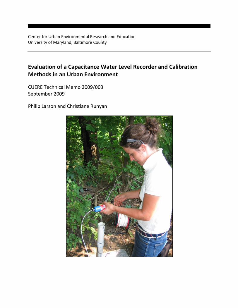
ON THE COVER Christiane Runyan maintaining an Odyssey capacitance water level recorder at Site 7, October 9, 2008. Photograph by Stuart Schwartz.

http://www.umbc.edu/cuere/BaltimoreWTB/

i

Table of Contents

Page Figures iii Tables iv Appendices v 1. Introduction 1

1.1 Background 1

1.2 Capacitance and Principles of Operation 1

1.3 Field Observations leading to this work 2

2. Sources of Error 3

2.1 Calibration 3

2.1.1 Methods 3

2.1.1.1 Bucket Method 3

2.1.1.2 PVC Pipe Method 4

2.1.1.2.1 Two Point Calibration 4

2.1.1.2.2 Multiple Point Calibration 5

2.1.1.2.3 Methods Used to Obtain Calibration Curves 5

2.1.1.2.4 Measurement Error 5

2.1.1.2.5 Native Groundwater Lab Calibration 8

2.1.1.2.6 Native Groundwater Field Calibration 8

2.1.2 Results 8



2.1.2.2.1 Two-Point Calibration 10

2.1.2.2.2 Multiple Point Calibration 10

2.1.2.2.3 Native Groundwater Lab Calibration 10

2.1.2.2.4 Native Groundwater Field Calibration 10

2.1.3 Discussion 11



2.1.3.3 Native Groundwater Lab Calibration 11

2.1.3.4 Native Groundwater Field Calibration 12

2.2 Calibration Precision, Linearity and Curvature 12

2.2.1 Methods 12

ii

2.2.2 Results 12

2.2.3 Discussion 15

2.3 Electrical Conductivity 16

2.3.1 Methods 16

2.3.2 Results 17

2.3.3 Discussion 19

2.4 Temperature 20

2.4.1 Methods 20

2.4.2 Results 20

2.4.3 Discussion 20

2.5 Film 23

2.5.1 Background 23

2.5.2 Methods 23

2.5.3 Results 23

2.5.4 Discussion 24

2.6 Physical Interferences 25

2.6.1 Methods 25

2.6.2 Results 25

2.6.3 Discussion 25

2.7 Other Sources of Error 25

2.7.1 Sensor Drift 25

2.7.1.1 Methods 25

2.7.1.2 Results 26

2.7.1.3 Discussion 26

2.7.2 Experimental Error 26

3. Summary, Conclusions, Recommendations 27

4. References 28

iii

Figures

Page Figure 1. Odyssey Capacitance Water Level Probe. 1

Figure 2. Schematic of a parallel plate capacitor with a dielectric (orange) between its two plates (grey lines). 1

Figure 3. Two-Point Fitting Error at Site 9. 13 Figure 4. Two-Point Fitting Error at Site 10. 14 Figure 5. Two-Point Fitting Error at Site 1. 14 Figure 6. Two-Point Fitting Error at Site 30. 15 Figure 7. Effect of electrical conductivity on raw value at three different depths

(Site 20 probe; S/N 33829). 17 Figure 8. The nonlinear fitting error at 1061 mm DTW in six different

conductivities shows that the Raw-DTW relationship becomes asymptotically more linear as conductivity increases. The low error at 510 μS/cm is likely a measurement error during the laboratory testing. □ is the estimated value at 510 μS/cm. 19

Figure 9. Effect of water temperature on capacitance probe raw value at two

water constant water levels (Site 9 probe; S/N 33830). 20 Figure 10. Groundwater temperatures at three capacitance-probe sites show

shallow groundwater is buffered from daily air temperatures. 21 Figure 11. Estimated DTW error range attributable to four error sources. 21 Figure 12. Calibration curves of Site 30 capacitance probe with and without film. 24 Figure 13. The sensor element of an Odyssey probe retains its coiled memory

and any additional kinks that could cause measurement error if in contact with the well casing. 25

iv

Tables

Page Table 1. Water level measurement discrepancy observed when using Bucket Method

calibration. Negative values indicate a capacitance probe reading at a smaller DTW than the e-tape reading. 2

Table 2. Calibration parameters for all calibrations performed on all probes. 6,7 Table 3. The minimum, maximum and median of the absolute median method error

for each calibration performed with the listed method. 8 Table 4. Measurement error of the Bucket calibration and the top two non-bucket

method calibrations for each site (excluding NGF calibrations). 9 Table 5. Range in electrical conductivity observed at each field site (May, 2009) and

associated sensed DTW error (Variation is estimated from Table 6 assuming a calibration slope of 2). 17

Table 6. Conductivity effects on probe raw values and their propagated effects on

calibration curve DTW. 18 Table 7. Temperature effects on Odyssey raw values and their propagated effects on

the calibration curve DTW values. 22 Table 8. Effects of film accumulation on probe performance. 23 Table 9. Effect of physical contact between the sensor element and various materials.

The DTW less than no-contact-DTW was approximated using a calibration slope of 2. 26

v

Appendices

Page Appendix A. Calibration and Curve Fitting 29

1

Figure 2. Odyssey capacitance water level probe.

Figure 3. Schematic of a parallel plate capacitor with a dielectric (orange) between its two plates (grey lines).

1. Introduction 1.1 Background Seven shallow wells were augered during the summer of 2007 and one during the summer of 2008 for the purpose of observing shallow groundwater levels in the riparian zone of DR3, DR4 and DR5 tributaries of the Dead Run subwatershed of the Gwynns Falls in Baltimore County, Maryland. A 2-m (7.7 ft, end-to-end) capacitance water level probe (Odyssey by Dataflow Systems Pty Ltd, Christchurch, New Zealand, http://www.odysseydatarecording.com, Figure 1) was installed in each shallow well. Including above ground casing, the average casing depth of the shallow wells was 8.4 feet.

Prior to deployment, each of the Odyssey capacitance probes (hereinafter referred to as capacitance probes) was calibrated in the lab using the “Bucket Method”, which is described in further detail in Section 2.1.1. Considerations during installation design included central placement of the capacitance probe within the well to avoid contact between the probe and the PVC casing, and vertical placement within the casing so the counterweight hung 0.3 ft above the bottom of the casing. Installation of the capacitance probes occurred during the second and third weeks of June 2008. At the time of deployment, a water level measurement was made at each site using an electronic water level measurement device, often referred to as an electronic tape or e-tape (Model 101 Water Level Meter, Solinst Canada, LTD.). The capacitance probes were installed to measure depth to water (DTW) below the probe’s O-ring seat at a 10-minute interval. Site maintenance was scheduled for a six-week interval. Site maintenance included measurement of the water level using the e-tape and downloading data collected over the six-week interval. 1.2 Capacitance and Principles of Operation Capacitance is the amount of charge that can be stored on a surface before the charge is able to overcome a less conductive material (dielectric) in an electrical circuit to jump the stored charge across the material to a second surface that will complete the circuit (Figure 2). Capacitance is defined as: C = εrε0 (A/d) (1) where C is capacitance [Farad], A is the area of each plate [m2], εr is the dielectric constant of the material between plates [dimensionless], ε0 is the dielectric constant of the vacuum of free space [Farad m-¹], and

2

Table 1. Water level measurement discrepancy observed when using Bucket Method calibration. Negative values indicate a capacitance probe reading at a smaller DTW than the e-tape reading.

Location Minimum

(mm) Median

(mm) Maximum

(mm)

Site 1 -40 -3 79

Site 7 -445 -285 -225

Site 8 -107 -19 99

Site 9 -191 -114 -107

Site 10 -25 12 27

Site 16 -56 -37 11

Site 20 -65 -43 -19

Site 30 -73 -21 12

d is the separation distance [m] between the plates. The relationships of these variables to capacitance are described here to aid the reader in understanding the basis of the capacitance probe’s operation. As the size of the plate increases, the amount of stored charge also increases, which results in increased capacitance. When a charge develops on the plates, the molecules of the dielectric material become polarized thereby decreasing the electric field surrounding the plates and increasing capacitance by allowing a larger positive (+) charge on the first plate to exist next to a larger negative (-) charge on the second plate. The relationship between distance separating the two plates and capacitance is inverse, such that an increased distance between plates results in decreased capacitance (Serway and Jewett, 2002). The principle of capacitance can be used to indirectly determine DTW, because the probe’s Teflon-covered element acts as the first capacitor plate, water acts as the second capacitor plate (connected to the electrical circuit through the counterweight and a second element beneath the Teflon) and the Teflon is the dielectric between the plates. The two elements and the Teflon dielectric are collectively referred to as the sensor element. The area of the first plate, distance between plates and the Teflon’s dielectric properties are constant, whereas the area of the second plate is proportional to water level and capacitance (Dataflow Systems 2008a). The capacitance probe outputs a unit of measure termed “raw value” that is proportional to capacitance and therefore increases as DTW decreases. 1.3 Field Observations Leading to this Work Following the second site visit, a difference between capacitance probe-sensed DTW and electronic tape-measured DTW was observed (Table 1). The manufacturer specifies that properly maintained probes have a resolution of 0.8 mm and can achieve ±5 mm accuracy (Dataflow Systems 2008c). The discrepancy between capacitance probe and measured DTW was variable between sites and in most cases the error exceeded the resolution ± the accuracy. This prompted an investigation to determine the sources of error. Six to eight weeks following installation of the capacitance probes, a rusty-orange film was observed to be coating the submerged Teflon dielectric of the capacitance probes at five out of eight sites. (The three sites where film was not observed were Sites 8, 9 and 20.) The absence of film at Site 8 was hypothesized as being due to its high average DTW, because the sensor element was not submerged and therefore would not allow film accumulation to occur. During site visits following the discovery of film accumulation on the sensor elements, film was cleaned

3

from the capacitance probes in accordance with the manufacturer’s specified procedure to use either a paper towel and DI water or a mild solution of detergent and DI water. 2. Sources of Error In order to determine the source of error between measured and sensed DTW, we examined the effects of water conductivity, water temperature, calibration method, curve fitting and physical interferences. 2.1 Calibration 2.1.1 Methods 2.1.1.1 Bucket Method The capacitance probes were originally calibrated in a bucket, as shown in the version of the

Odyssey manual shipped with the probes on March 22, 2008 (Dataflow Systems 2008a), filled

with deionized (DI) water (< 2 microSiemens (µS)/cm) at room temperature (≈20 ˚C) to obtain a

raw value proportional to capacitance at both a low and high water level on the sensor

element. This method, which we refer to as the “Bucket Method” consists of the following

steps:

Mark two points on the surface of the cleaned Teflon sensor element with a waterproof pen, one ≈2100 mm down from the O-ring seat and the second ≈320 mm down from the O-ring seat.

Using the supplied data cable, connect the capacitance probe to the communications (COM) port on the computer. Next, start the Odyssey data program and select “probe trace” (data streaming) mode.

Submerge the probe into a 5 gallon bucket filled with about 4 gallons of DI water up to the first point (2100 mm) and record the number on the screen once a constant value has been reached.

Continue to submerge the sensor element until the meniscus of the next point (320 mm) is reached. It is necessary to coil the sensor element in order to achieve full submersion, however, the sensor can be damaged if the coiled diameter is less than 100mm (Dataflow Systems 2008a).

Hold the blue datalogger enclosure stable at this point and record the raw value on the screen once a constant value has been reached (this will be the first number entered into the uncalibrated data value column, while the first recorded value will be the second entered value).

The two-point linear calibration formula is determined from the following equations:

Calibrated Water Level (WL) Value = ((Raw Value) – (Offset))/(Slope) (2) Slope = (High Raw WL – Low WL Raw)/(High Measured DTW – Low Measured DTW) (3)

4

Offset = (High Raw WL)-(High Measured DTW * Slope) (4)

The measurement error for the bucket method is calculated by obtaining the difference between bucket-calibrated DTW and the DTW obtained from the e-tape. The number of DTW measurements and therefore the number of times the measurement error was calculated was different for each site, but varied between 10 and 19 DTW measurements. Statistical analysis of the absolute measurement error using the average, median, standard deviation, sum of the squared errors (SSE) and minimum and maximum errors were computed to compare measurement errors and to determine the optimal calibration method. The sum of the squared errors was used to rank the calibrations for each site. The method’s accuracy can be defined by the median of the median measurement errors, which can also be used to rank the methods. The measurement error is defined as

Measurement error = (calibration DTW) – (field-measured DTW) (5) The effect of calibrating the probe coiled and in contact with the bucket was compared to calibrating the probe uncoiled and hanging freely in a well casing by computing the difference between the calibration DTW values. A Bucket Method calibration was performed and the raw value corresponding to a DTW of 320 mm was recorded for multiple configurations of the coiled sensor element in contact with the bucket. The raw value at 320 mm DTW was also recorded for a probe coiled into 200 mm diameter loops and tied and suspended with PVC ribbon in water but without contacting the bucket. A probe hanging in a well casing in the lab was calibrated in DI water using the PVC Pipe Two-Point Method. 2.1.1.2 PVC Pipe Method 2.1.1.2.1 Two-Point Calibration Two Bucket Method calibration error sources were hypothesized to be: (1) calibrating probes in DI water and (2) the dielectric being in contact with a surface (the side of the bucket) other than that of water. This prompted re-calibration of the probes using the method referred to as the PVC pipe two-point method, which is the manufacturer’s sole calibration method in a revised product manual received December 12, 2008 (Dataflow Systems 2008b). The conductivity of the calibration water was not specified in that manual but was chosen during our calibrations. The PVC Pipe Method consists of the following steps:

Mark two points on a clean surface of the Teflon sensor element with a waterproof pen, one 320 mm down from the O-ring seat and the second 2100 mm down from the O-ring seat.

Using the supplied data cable, connect the capacitance probe to the computer’s COM port, start the Odyssey data program and select “probe trace” mode.

Secure a seven-foot PVC pipe with a diameter of at least 2 inches and a cap on its lower end next to a six-foot shelf in the lab with cable ties to ensure that movement during the tests is minimized. Fill the pipe with water similar in conductivity to the probe’s

5

native groundwater to a level approximately 1 inch below the top of the casing. Suspend the probe using a clamp and ring stand on the shelf, submerge the probe to the 320 mm mark and record the raw value. Make sure the counterweight or the sensor element is not touching the pipe.

Follow the same procedure described in the previous step to obtain the raw value for the 2100 mm point, except using a ten-inch long PVC pipe.

The two-point linear calibration formula uses the same formulas as the bucket method.

Measurement error for the PVC Pipe Two-Point method was calculated using Equation 5.

2.1.1.2.2 Multiple Point Calibration The Odyssey probe manual states that the probe is a linear measuring device but that very low conductivity water may result in a nonlinear calibration (Dataflow Systems 2008a). Large measurement errors and the possibility of a nonlinear raw-DTW relationship prompted calibration using the PVC Pipe Multiple Point Method and quantification of nonlinear calibration error. The PVC Multiple Point Method expands on the PVC Pipe Two-Point Method to include collecting raw values along the length of the probe by way of the following steps:

Secure a seven-foot PVC pipe in the lab next to a shelf with cable ties to ensure that movement during the tests is minimized.

Fill the PVC pipe with water of a known conductivity and secure the capacitance probe so it will not move throughout the duration of the test.

Connect the capacitance probe to the Odyssey program and enter “probe trace” mode. The stabilized raw value should be entered into a spreadsheet.

Following each measurement, obtain a water level measurement to the nearest 0.01 ft from the O-ring seat to the water level using an e-tape.

Use a siphon to remove water from the PVC pipe to obtain a minimum of 10 evenly distributed measurements over the length of the sensor element. Two of these ten measurements should be the two points obtained in the PVC Two-Point Method.

2.1.1.2.3 Methods Used to Obtain Calibration Curves Least squares linear regression and a least squares polynomial regression were used to obtain calibration curves for calibrations conducted using the PVC Multiple Point Method. 2.1.1.2.4 Measurement Error The measurement error for the PVC Multiple Point Method was calculated for the linear and polynomial regression using the same process as the PVC Two-Point measurement error.

6

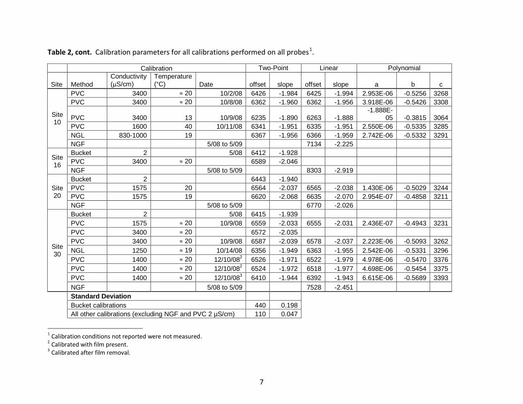
Table 2. Calibration parameters for all calibrations performed on all probes1.

Calibration Two-Point Linear Polynomial

Site Method

Conductivity (μS/cm)

Temperature (°C) Date offset slope offset slope a b c

Site 1

Bucket 2 5/08 6358 -1.874

PVC 870 ≈ 20 12/12/082 6498 -1.963 6493 -1.983 6.055E-06 -0.5565 3380

PVC 870 ≈ 20 12/12/083 6480 -1.975 6462 -1.972 5.512E-06 -0.5524 3360

PVC 870 ≈ 20 12/12/083 6471 -1.967 6464 -1.972 4.866E-06 -0.5480 3355

NGF 5/08 to 5/09 6900 -2.092

Site 7

Bucket 2 5/08 5247 -1.407

PVC 2 4/16/09 2731 -0.2168

PVC 765 ≈ 20 6528 -2.013

PVC 3400 ≈ 20 6564 -2.037

PVC 3400 ≈ 20 10/18/08 6562 -2.044 6559 -2.041 -4.196E-07 -0.4866 3208

NGF 5/08 to 5/09 7072 -2.137

Site 8

Bucket 2 5/08 6419 -1.935

NGF 5/08 to 5/09 6820 -1.997

Site 9

Bucket 2 5/08 5771 -1.638

PVC 2 9/30/08 3625 -0.6162

PVC 320 ≈ 20 9/29/08 6411 -1.955 6437 -1.955 -1.052E-05 -0.4246 3133

PVC 765 ≈ 20 9/30/08 6568 -2.035 6568 -2.026 -3.349E-06 -0.4654 3189

PVC 1575 ≈ 20 10/2/08 6589 -2.045 6574 -2.058 5.946E-06 -0.5335 3285

PVC 1575 19.5 10/12/08 6536 -2.027 6543 -2.022 -5.030E-06 -0.4534 3161

PVC 3400 ≈ 20 10/2/08 6605 -2.051 6610 -2.051 -1.194E-06 -0.4778 3205

NGL 855-1163 12.8 10/12/08 6669 -2.066 6622 -2.045 1.376E-06 -0.5000 3258

NGL 820 18 10/13/08 6703 -2.073 6666 -2.057 3.042E-06 -0.5104 3284

NGF 5/08 to 5/09 7341 -2.379

Site 10

Bucket 2 5/08 6406 -1.944

PVC 765 ≈ 20 9/28/08 6370 -1.959 6368 -1.951 -2.011E-06 -0.4965 3235

PVC 1575 ≈ 20 10/2/08 6394 -1.970 6394 -1.989 5.274E-06 -0.5446 3291

1 Calibration conditions not reported were not measured.

2 Calibrated with film present. 3 Calibrated after film removal.

7

Table 2, cont. Calibration parameters for all calibrations performed on all probes1.

Calibration Two-Point Linear Polynomial

Site Method


Temperature (°C) Date offset slope offset slope a b c

Site 10

PVC 3400 ≈ 20 10/2/08 6426 -1.984 6425 -1.994 2.953E-06 -0.5256 3268

PVC 3400 ≈ 20 10/8/08 6362 -1.960 6362 -1.956 3.918E-06 -0.5426 3308

PVC 3400 13 10/9/08 6235 -1.890 6263 -1.888 -1.888E-

05 -0.3815 3064

PVC 1600 40 10/11/08 6341 -1.951 6335 -1.951 2.550E-06 -0.5335 3285

NGL 830-1000 19 6367 -1.956 6366 -1.959 2.742E-06 -0.5332 3291

NGF 5/08 to 5/09 7134 -2.225

Site 16

Bucket 2 5/08 6412 -1.928

PVC 3400 ≈ 20 6589 -2.046

NGF 5/08 to 5/09 8303 -2.919

Site 20

Bucket 2 6443 -1.940

PVC 1575 20 6564 -2.037 6565 -2.038 1.430E-06 -0.5029 3244

PVC 1575 19 6620 -2.068 6635 -2.070 2.954E-07 -0.4858 3211

NGF 5/08 to 5/09 6770 -2.026

Site 30

Bucket 2 5/08 6415 -1.939

PVC 1575 ≈ 20 10/9/08 6559 -2.033 6555 -2.031 2.436E-07 -0.4943 3231

PVC 3400 ≈ 20 6572 -2.035

PVC 3400 ≈ 20 10/9/08 6587 -2.039 6578 -2.037 2.223E-06 -0.5093 3262

NGL 1250 ≈ 19 10/14/08 6356 -1.949 6363 -1.955 2.542E-06 -0.5331 3296

PVC 1400 ≈ 20 12/10/082 6526 -1.971 6522 -1.979 4.978E-06 -0.5470 3376

PVC 1400 ≈ 20 12/10/082 6524 -1.972 6518 -1.977 4.698E-06 -0.5454 3375

PVC 1400 ≈ 20 12/10/083 6410 -1.944 6392 -1.943 6.615E-06 -0.5689 3393

NGF 5/08 to 5/09 7528 -2.451

Standard Deviation

Bucket calibrations 440 0.198

All other calibrations (excluding NGF and PVC 2 µS/cm) 110 0.047



8

Table 3. The minimum, maximum and median of the absolute median method error for each calibration performed with the listed method.

Method error (mm) Bucket PVC 2pt

PVC linear

PVC poly

NGL 2pt

NGL linear

NGL poly

NGF linear

Minimum median 11 12 12 11 6 4 30 59

Median median 29 27 29 66 14 19 44 92

Maximum median 288 81 80 195 58 59 96 233

2.1.1.2.5 Native Groundwater Lab Calibration Three sensors were calibrated with groundwater obtained from their respective field sites (Sites 9, 30, and 10) to examine the effect of groundwater chemistry on probe performance. Groundwater was pumped from the wells using an ISCO 6712 and was brought back to the lab for use in a PVC Multiple-Point calibration. Native Groundwater Lab (NGL) calibration curves were developed and measurement error was calculated using the same methods as the PVC Multiple Point method. 2.1.1.2.6 Native Groundwater Field Calibration The Native Groundwater Field (NGF) calibration method uses a linear regression between raw value and DTW data collected during the field maintenance procedure. An e-tape was used to measure DTW to the nearest 0.01 ft from a consistent measurement point on the well casing. The last raw value logged before maintenance and the first raw value logged after maintenance were assumed to be representative of the raw value at the time of measured DTW. This was typically less than 30 minutes. Pre- and post-maintenance raw values were used as discrete data points to compute the NGF calibration curve. Measurement error was calculated using Equation 5. 2.1.2 Results 2.1.2.1 Bucket Method A list of all calibrations performed on each probe along with the calibration curve parameters are listed in Table 2. Error statistics are summarized in Table 3. The median (x)̃ Bucket Method error of all the sites varied from 11 to 288 mm. The minimum median and median median of all Bucket Method errors was nearly equal to that of the PVC Two-Point Method. The largest median bucket error was 288 mm and occurred at Site 7. This was the second largest median error among all the calibration methods, which included PVC two-point, PVC linear, PVC polynomial, NGL and NGF measurement errors. Various configurations of the sensor element coiled in the bucket ranged from 5200 to 5750 raw value. Calibrations developed from the maximum and minimum raw value of this range would differ in their sensed DTW by 325 mm. A coiled suspended sensor element measured a consistent raw value of 5700. Calibrating probes hanging in a well casing resulted in measurement errors larger than 900 mm and is much different compared to the largest Bucket Method error of -445 mm (Table 1).

9

Table 4. Measurement error of the Bucket calibration and the top two non-bucket method calibrations for each site (excluding NGF calibrations)1.

Site and average conductivity

Calibration Method

Conductivity

(μS/cm)

Temperature

(°C) Date

Maximum Error (mm)

Minimum Error (mm)

Average Error (mm)

Median Error (mm)

Rank (lowest error)

Site 1 (840 µS/cm)

Bucket two-point 2 μS/cm 5/08 79 -40 2 -3 1 of 13

PVC two-point 870 µS/cm ≈20°C 12/12/083 72 -59 -7 -8 2 of 13

PVC two-point 870 µS/cm ≈20°C 12/12/083 77 -60 -7 -7 3 of 13

Site 7 (3482 µS/cm)

Bucket two-point 2 μS/cm 5/08 -225 -445 -308 -285 5 of 7

PVC two-point 765 μS/cm ≈20°C 2 -10 -164 -78 -66 1 of 7

PVC two-point 3400 μS/cm ≈20°C 3 -10 -164 -79 -68 2 of 7

Site 8 (1387 µS/cm) Bucket two-point 2 μS/cm 5/08 99 -107 -32 -19 1 of 1

Site 9 (861 µS/cm)


ISGL two-point 820 μS/cm 18°C 10/13/08 8 -16 -1 1 1 of 25

ISGL linear 820 μS/cm 18°C 10/13/08 3 -21 -6 -4 2 of 25


Bucket two-point 2 μS/cm 5/08 27 -25 11 12 2 of 24

PVC polynomial 765 μS/cm ≈20°C 9/28/08 24 -30 7 9 1 of 24

PVC two-point 3400 μS/cm ≈20°C 10/2/08 2 -50 -14 -12 3 of 24


Bucket two-point 2 μS/cm 5/08 11 -56 -32 -37 2 of 2

PVC two-point 3400 μS/cm ≈20°C 13 -59 -26 -23 1 of 2



PVC linear 1575 µS/cm 19°C 10/11/08 -8 -50 -26 -28 1 of 9

PVC polynomial 1575 µS/cm 19°C 10/11/08 -16 -54 -32 -34 2 of 9


Bucket two-point 2 μS/cm 5/08 12 -73 -24 -21 9 of 22

PVC linear 1400 µS/cm ≈20°C 12/10/082 37 -50 0 2 1 of 22

PVC linear 1400 µS/cm ≈20°C 12/10/082 37 -50 1 3 2 of 22



10

2.1.2.2 PVC Pipe Method 2.1.2.2.1 Two-Point Calibration Not all PVC Two-Point calibrations at each site had a lower measurement error than the site’s Bucket Method calibration. The PVC Two-Point was the best calibration at Sites 7 and 16, and in comparison to other calibration methods was the third most accurate (x ̃= 27 mm) (Table 4 and Table 3). It should be noted that more PVC Two-Point Method calibrations were performed than any other method because they are the quickest and simplest calibration method (Table 2). The PVC Two-Point calibration with the largest error was 92 mm, occurring at Site 7. 2.1.2.2.2 Multiple Point Calibration At Sites 20 and 30, the PVC Multiple Point Method using a linear regression had the lowest measurement error and in comparison to other calibration methods was the fourth most accurate (x ̃= 29 mm) (Table 4). The overall accuracy of the PVC linear regression was nearly equal to the Two-Point method (Table 3). Visual inspection of the PVC Multiple Point calibrations indicated a nonlinear relationship between raw value and depth to water that is examined in more detail in Section 2.2. The Multiple Point Method obtained the lowest error at Site 10 using a polynomial regression. The polynomial measurement error ranked sixth in comparison to other calibration methods and had twice the error of the other PVC methods (Table 3). 2.1.2.2.3 Native Groundwater Lab Calibration The NGL Method was performed for Sites 9, 10, and 30 using a two-point fit, linear regression and polynomial regression. This method resulted in the lowest measurement error of all the calibrations at Site 9 but greater error than the majority of PVC calibrations at Site 10 and the PVC and Bucket calibrations at Site 30. The NGL two-point calibration had the lowest measurement error in comparison to other calibration methods (x ̃= 14 mm) (Table 3). The most accurate individual calibration was obtained by an NGL linear regression at Site 9 with a median measurement error of 4 mm (Table 4). The NGL calibration slope and offset of the raw-DTW relationship differed from PVC calibrations using the same probe and a similar conductivity DI-KCl solution. Two of the three NGL calibrations had a more negative slope and a higher offset than PVC calibrations of approximately equal conductivity (Table 2). At Site 9, the raw-DTW relationship of NGL calibrations had convex curvature to the origin whereas five out of the six PVC calibrations had concave curvature (Figure 3). 2.1.2.2.4 Native Groundwater Field Calibration The NGF method was used to develop calibrations for all eight sites and consistently had higher measurement errors than other calibration methods. The NGF calibration uses raw-DTW data from the bottom 3.5 feet or less of the sensor element owing to the limited range of water levels in the riparian wells.

11

2.1.3 Discussion 2.1.3.1 Bucket Method Bucket-derived calibration curves varied in their predictive DTW capabilities when applied to raw field values. The measurement error was not consistent across capacitance probes in underprediction, overprediction or magnitude. The large range in raw values obtained from a coiled probe in a water-filled bucket shows that probes are affected by contact with the bucket and that this technique produces inconsistent calibrations. In comparison to the bucket method, the PVC Pipe Methods are assumed to be superior calibration methods because they better emulate field conditions with respect to probe position and water conductivity. The large difference in measurement errors between the PVC Two-Point Method and Bucket Method calibrations in 2 µS/cm water shows that the sensor element’s position during the Bucket Method calibration creates an inaccurate calibration and therefore is not a recommended calibration method. However, some bucket method calibrations are unexplainably, perhaps coincidentally, comparable in accuracy to the PVC pipe method. 2.1.3.2 PVC Pipe Method Similar to the Bucket Method, none of the four types of PVC Pipe calibration methods, which includes the Two-Point, Multiple Point and NGL or NGF, obtained a consistent measurement error. For 72 out of 121 or 60% of PVC Pipe calibrations, this error was larger than the Bucket Method error despite the method being more similar to field-deployed conditions. However, PVC Pipe calibrations can be characterized as being most consistent because they have a smaller standard deviation for calibration parameters (Table 2). Since PVC and NGL polynomial calibrations did not consistently obtain a measurement error lower than the two-point or linear calibrations, we suspect that polynomial calibrations define the raw-DTW relationship accurately for only a small range of environmental conditions. Two-point calibrations obtain a lower median measurement error and are better than polynomial calibrations when environmental conditions vary. We examine and discuss the significance of curve fitting in Section 2.2. 2.1.3.3 Native Groundwater Lab Calibration The differences between NGL slope and offset contradict our results from Section 2.3 and 2.4 that show that calibration slope and offset increase as conductivity increases and decrease as temperature increases from 13 to 18°C. Slope and offset are expected to increase as conductivity increases. These observations suggest that groundwater properties in addition to conductivity and temperature can influence the raw value and the performance of the probe. Calibration curvature, slope and offset are discussed in further detail in Section 2.2. Despite the NGL method obtaining the most accurate calibration, its measurement error is larger than the probe’s specified accuracy. Our confidence in the accuracy of the NGL method is limited because it was executed only three times compared to the PVC Two-Point Method’s 28 times. More calibrations using the NGL method could provide a better understanding of its

12

accuracy. Nonetheless, we believe that calibrating the probes using native groundwater provides the most accurate calibration but that the accuracy of the probes is limited by external variables discussed later. 2.1.3.4 Native Groundwater Field Calibration The NGF is not a recommended calibration method due to its high measurement error. It may prove to be more useful if e-tape measurements were obtained over a greater range of DTW thereby better defining the raw value-DTW relationship. 2.2 Calibration Precision, Linearity and Curvature 2.2.1 Methods The precision of the PVC Two-Point calibration method was determined by comparing sensed DTW values for calibrations performed under nearly identical conductivity and temperature conditions. The difference between each calibration’s sensed DTW was computed for a high (2150), medium (3500) and low (6200) DTW (raw value). (High capacitance is associated with low DTW (high water table)). The Odyssey manual states that calibrations should result in an offset within 20 raw values of the offset from other calibrations obtained with the probe (Dataflow Systems 2008a). Differences between offset values from PVC Pipe Two-Point calibrations above 2 μS/cm, excluding film and native groundwater calibrations, were computed for each probe. The conductivity and temperature of calibration water were not measured before the start of most calibrations but these properties were sometimes measured and recorded at the beginning of the test day. Calibrations performed at assumed equal conductivities and immediately following one another are termed replicate and duplicate calibrations, respectively. The capacitance probe is a nonlinear measuring device in low conductivity water as mentioned in previous sections and alluded to in the Odyssey manual (Dataflow Systems 2008a). The measurement error due to using a Two-Point calibration for low conductivity water was determined by computing its nonlinear fitting error. Curvature (a positive two-point fitting error represents a raw-DTW relationship that is concave with respect to the origin), distribution of error along the length of the probe, and linearity of the raw-DTW relationship were examined visually over a range of conductivities, temperature and water chemistry using the two-point fitting error. We considered calibrations with two-point fitting errors less than ± 5 mm to be linear. The nonlinear and two-point fitting errors were calculated for all PVC Multiple Point and NGL calibrations using the following formulas: Nonlinear Fitting Error (mm) = (Two-Point DTW) – (Polynomial DTW) (6) Two-Point Fitting Error (mm) = (Measured DTW when calibrating) – (Two-Point DTW) (7) 2.2.2 Results Raw-DTW relationships and their calibration curve parameters obtained over a range of conditions were often not reproducible and exhibited differences in the slope and offset, linearity and curvature of the raw-DTW relationship. Calibrations conducted in higher

13

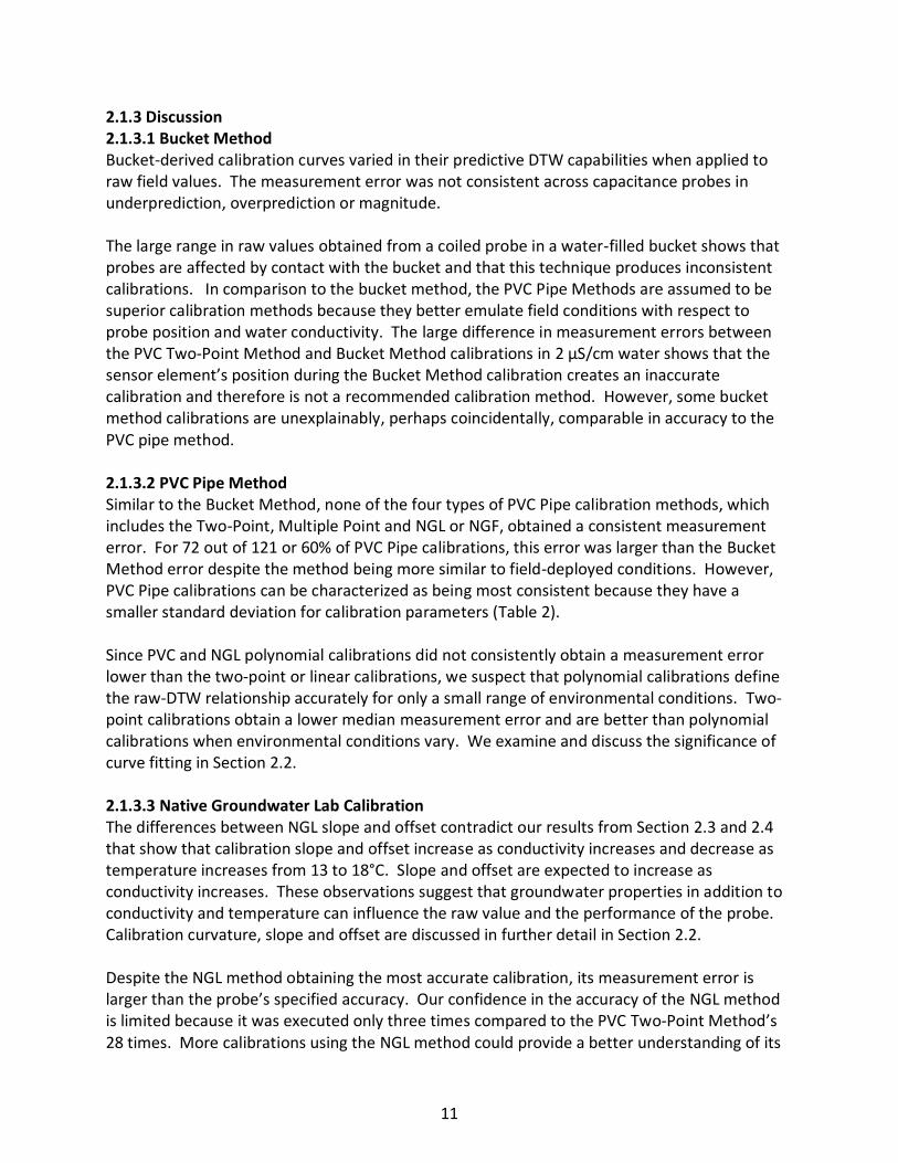
conductivity water usually resulted in greater sensed DTW values (evidenced by the greater slope and offset) than lower conductivity calibrations, although a few calibrations had a lower slope and offset (Table 2). Differences in the slope and offset of replicate calibrations (n = 4 sets of 2) resulted in a difference of sensed DTW from 1 to 30 mm (x ̃= 6 mm). These differences increase as DTW decreases. Duplicates (n = 3 sets of 2) differed in sensed DTW from 0 to 24 mm (x ̃= 2). Two duplicates and one replicate differed by less than or equal to the manufacturer’s specified ±5 mm probe accuracy. The largest difference between probes’ calibration offsets ranged from 28 to 63 raw values. Some replicate and duplicate calibration offsets also deviated by more than 20 raw values and differed by 2 to 63 for the former and by 2 to 55 raw values for the latter (Table 2). The shape of the raw-DTW relationship varied in concave or convex curvature and in location of greatest error along the probe (distribution of error ranged from left to normal to right skew). At Site 9, NGL calibrations are examples of calibrations with left skew and convex curvature (Figure 3). All but one PVC Pipe calibration at Site 9 had a normal distribution of error and concave curvature. The majority of calibrations at Site 10 have right skew and convex curvature (Figure 4). Calibrations with film accumulation have right skew, corresponding to the location of the film accumulation on the sensor element (Figure 5 and Figure 6). Due to this nonlinearity, using a polynomial fit for all of the PVC Multiple Point calibrations listed in Table 2 instead of a Two-Point calibration reduced a maximum nonlinear error of 53 mm and median maximum error of 11 mm. Linear regression curves reduce less error than polynomial curves but still have a lower SSE than two-point curves. Also, a small amount of

Figure 3. Two-Point Fitting Error at Site 9.

-1650

-1500

-1350

-1200

-1050

-900

-750

-600

-450

-300

-150

0

150

300

450

600

750

900

1050

-60

-50

-40

-30

-20

-10

0

10

20

30

40

0 500 1000 1500 2000

Two

-Po

int

Fitt

ing

erro

r fo

r P

VC

2μ

S/cm

(mm

)

Two

-Po

int

Fitt

ing

Erro

r (m

m)

Measured DTW (mm)

PVC, 320 μS/cm, ≈20°C, 9/29/09PVC, 765 μS/cm, ≈20°C, 9/30/08PVC, 1575 μS/cm, 19.5°C, 10/12/08PVC, 1575 μS/cm, ≈20°C, 10/2/08PVC, 3400 μS/cm, ≈20°C, 10/2/08NGL, 855-1163 μS/cm, 12.8°C, 10/12/08NGL, 820 μS/cm, 18°C, 10/13/08PVC, 2 μS/cm, 5/08

14

Figure 4. Two-Point fitting error at Site 10.

-30

-20

-10

0

10

20

30

40

50

60

70

0 500 1000 1500 2000 2500

Two

-Po

int F

itti

ng

Erro

r (m

m)

Measured DTW (mm)

PVC, 765 μS/cm, ≈20°C, 9/28/08PVC, 1575 μS/cm, ≈20°C, 10/2/08PVC, 3400 μS/cm, ≈20°C, 10/2/08PVC, 3400 μS/cm, 13°C, 10/9/08PVC, 3400 μS/cm, ≈20°C, 10/8/08PVC, 1600 μS/cm, 40°C, 10/11/08NGL, 830-1000 μS/cm, 19°C, 10/14/08


-50

-40

-30

-20

-10

0

10

20

30

40

50

0 500 1000 1500 2000 2500

Two

-Po

int F

itti

ng

Erro

r (m

m)

Measured DTW (mm)

PVC (with film), 870 µS/cm, 12/12/08

PVC (without film), 870 µS/cm, 12/12/08


15


-50

-40

-30

-20

-10

0

10

20

30

40

50

0 500 1000 1500 2000 2500

Two

-Po

int F

itti

n E

rro

r (

mm

)

Measured DTW (mm)

PVC, 1575 μS/cm, ≈20°C, 10/9/08

PVC, 3400 μS/cm, ≈20°C, 10/9/08

ISGL, 1250 μS/cm, ≈19°C, 10/14/08




evidence supports the use of a polynomial curve if the groundwater temperature remains near 13°C, as one of the two calibrations performed near 13°C is much less linear than at 20°C (Figure 4). Twenty-one out of twenty-five or 84% of the PVC Multiple Point calibrations had nonlinear errors larger than 5 mm. Two of the five calibrations at the highest calibration conductivity, 3400 µS/cm, had nonlinear errors less than 5 mm; however, no PVC Multiple Point calibrations were performed using water above 3400 µS/cm. Results from Section 2.3 show calibrations above 2100 µS/cm have less than 5 mm nonlinear fitting error. 2.2.3 Discussion Replicate calibrations differing in sensed DTW by more than 5 mm and in offset values by more than 20 raw values show that calibrations are not reproducible to the precision stated by the manufacturer. The precision of the Two-Point Method diminishes the accuracy of the probes and increases their measurement error to ± 24 mm. Since some replicate calibrations and two of the three duplicates differed by less than 5 mm in sensed DTW, additional duplicate calibrations should be performed to determine if 24 mm is the maximum difference between duplicate calibrations. Replicate calibrations verify a similar but slightly larger measurement error of ± 30 mm; however, these results are not reliable since the conductivity of the calibration water could have changed between replicates. Calibration water was stored over a two week period in uncovered five gallon buckets. Evaporation or particle deposition could have caused the conductivity of the water to change. However, a 30 mm difference between

16

calibrations corresponds to an 800 µS/cm difference in calibration water that was unlikely to occur from open storage. The distribution of the fitting error indicates the DTW where the probe will be least accurate if using a two-point fit. The location of greatest error and the importance of using the PVC Multiple Point method and a polynomial fit depend upon water chemistry, conductivity and temperature. More NGL calibrations are needed to determine whether the distribution of error in native groundwater, like that observed in Figure 3, are consistently different from DI-KCl calibrations. Recording the raw value at a third water level in the temperature test discussed in Section 2.4 is needed in order to determine the effect of temperature on linearity. From analysis conducted to date, conductivity appears to be the best indicator for determining whether a polynomial calibration is necessary. Based on our data, a polynomial regression should be used if conductivity is below 2100 µS/cm in order to obtain ± 5 mm accuracy. The improved accuracy of using a polynomial fit was only observed in the lab under a constant conductivity and was not found to be applicable in the field due to variable groundwater conductivity. 2.3 Electrical Conductivity 2.3.1 Methods The capacitance probe manual does not recommend any specifications regarding the chemistry of the calibration water nor does it specify the conductivity that may yield a nonlinear calibration (Dataflow Systems 2008b). To test for conductivity effects, capacitance probes were PVC Pipe-calibrated in water having conductivities of 320 (tap water), and KCl solutions of 765, 1575, 1600 and 3400 µS/cm. These values were chosen to correlate with the conductivity range of groundwater across sites at the time this work was completed (October 2008). As of May 2009, groundwater conductivity range was 175 to 6250 µS/cm across sites (Table 5). The tests for some probes were conducted for the purpose of obtaining a PVC Two -Point Method calibration, while others were conducted using the PVC Multiple Point Method for the purpose of creating or comparing between a two-point, linear or polynomial regression curve. All conductivity values were measured using a conductivity meter (Model DA-1 LaMotte Co., Chestertown, MD). To test solely for conductivity effects on raw value and to emulate the effect of changes in groundwater conductivity on sensed DTW, raw values were recorded at a constant water level while potassium chloride (KCl) was incrementally mixed into the water over a range in conductivities from 135 to 10000 µS/cm to bracket the range of field values measured in October 2008. This was performed with the sensor element submerged at: 15% (1878 mm), 55% (1061 mm) and 91% (326 mm) of its length (DTW). A two-point curve was developed using data collected at depths 1878 and 326 mm for each incremental increase between 135 and 10000 µS/cm. For each of these curves, sensed DTW values were computed for selected raw values between 2150 and 6200, which correspond approximately to the smallest and largest raw value that a two-meter capacitance probe can record. To quantify conductivity’s nonlinear effect, the difference was determined between the raw value recorded by the probe at the 1061 mm depth and the raw value back-calculated from a sensed DTW of 1061 mm using the two-point calibration curve for selected conductivities

17

Table 5. Range in electrical conductivity observed at each field site (May, 2009) and associated sensed DTW error (Variation is estimated from Table 6 assuming a calibration slope of 2).

Site Odyssey S/N

Minimum E.C. (µS/cm)

Maximum E.C. (µS/cm)

Sensed DTW (mm) variation due to range of groundwater conductivity

Site 1 33834 530 840 29

Site 7 33835 795 6250 40

Site 8 33833 590 1600 40

Site 9 33830 705 1000 15

Site 10 33828 670 1200 24

Site 16 33831 210 620 153

Site 20 33829 175 1950 240

Site 30 33832 920 3200 63

Figure 7. Effect of electrical conductivity on raw value at three different depths (Site 20 probe; S/N 33829).

2500

3000

3500

4000

4500

5000

5500

6000

0 2000 4000 6000 8000 10000

Raw

Va

lue


Raw value at 326mm DTW



between 135 and 10000 μS/cm (Equation 8). This difference in raw value was divided by the calibration slope to determine the difference in sensed DTW and the nonlinear error attributable to conductivity. Although calculated differently, this difference is comparable to the Two-Point Fitting Error and we distinguish these errors only by their equation. Two-Point Fitting Error (mm) = (Measured raw value when calibrating) – (Raw value back-calculated from 1061 mm using Two-Point calibration) / Slope (8)

2.3.2 Results The relationship between conductivity and raw value for three DTWs is presented in Figure 7. This figure shows that the raw value increases asymptotically with conductivity and that this effect varies with DTW. This indicates that probes are less sensitive in the upper range of conductivity, where small changes in raw value result from large changes in conductivity and the slope of the Raw Value-Conductivity relationship is near zero, compared to the lower range of conductivity where the slope of the Raw-Conductivity relationship is greater than zero. This behavior implies that probes used in high conductivity water can achieve ±5 mm accuracy over a larger range in

18

Table 6. Conductivity effects on probe raw values and their propagated effects on calibration curve DTW.

Conductivity Effects on Site 20 probe Site 20 probe raw values

2150 2739 3000 3500 4000 5000 5830 6200

E.C. (µS/cm)

Raw value 1878 mm

Raw value 326 mm Offset Slope Calibration Curve DTW (mm)

135 2735 5286 5822 -1.644 2234 1876 1717 1413 1108 500 -5 -230

205 2735 5521 6106 -1.795 2204 1876 1730 1452 1173 616 154 -52

310 2736 5690 6310 -1.903 2186 1876 1739 1477 1214 689 252 58

420 2738 5769 6406 -1.953 2179 1877 1744 1488 1232 720 295 105

510 2737 5803 6447 -1.976 2175 1877 1745 1492 1239 732 312 125

700 2738 5843 6495 -2.001 2172 1878 1747 1497 1247 747 332 148

805 2738 5862 6518 -2.013 2170 1878 1748 1499 1251 754 342 158

900 2738 5872 6530 -2.019 2169 1878 1748 1501 1253 758 347 164

1250 2738 5886 6547 -2.028 2168 1878 1749 1502 1256 763 354 171

1750 2739 5905 6570 -2.040 2167 1878 1750 1505 1260 770 363 181

2350 2739 5919 6587 -2.049 2165 1878 1751 1507 1263 775 369 189

3100 2741 5931 6601 -2.055 2166 1879 1752 1509 1265 779 375 195

4150 2741 5938 6610 -2.060 2165 1879 1752 1510 1267 781 378 199

5100 2741 5944 6617 -2.064 2164 1879 1753 1510 1268 783 381 202

6000 2741 5937 6608 -2.059 2165 1879 1752 1509 1267 781 378 198

7050 2741 5947 6620 -2.066 2164 1879 1753 1511 1269 784 383 204

8300 2741 5944 6617 -2.064 2164 1879 1753 1510 1268 783 381 202

10000 2741 5948 6622 -2.066 2164 1879 1753 1511 1269 785 383 204

Mean 2739 5830

6000-205 µS/cm DTW -39 3 22 58 93 165 224 251

10000-135 µS/cm DTW -70 3 36 98 160 285 388 434

19

Figure 8. The nonlinear fitting error at 1061 mm DTW in six different conductivities shows that the Raw-DTW relationship becomes asymptotically more linear as conductivity increases. The low error at 510 μS/cm is likely a measurement error during the laboratory testing. □ is the estimated value at 510 μS/cm.

0

20

40

60

80

100

120

0 2000 4000 6000 8000 10000

No

nli

near

Fit

tin

g E

rro

r (

mm

)


Nonlinear fitting error

Estimated error

5 mm of error

conductivity than probes used in lower conductivity water. This figure also suggests that it is important to calibrate probes in water with conductivity equal to the groundwater conductivity of the field site. Table 6 can be used to compute the range in conductivity over which a probe calibrated at a particular conductivity is able to achieve ±5 mm accuracy. Table 6 also shows that the greatest difference in sensed DTW occurs at larger raw values due to differences in calibration slope. At the site with the largest range in conductivity, Site 20, the error attributable to conductivity was approximately 240 mm (Table 5). The asymptotes observed at the three depths in Figure 7 do not span an equal

range in raw values. The raw-DTW relationship becomes more linear as conductivity increases, which can be verified by plotting the Two-Point Fitting Error against conductivity (Figure 8). A best-fit line estimates this error to be less than 5 mm for probes used in water above 2100 μS/cm. 2.3.3 Discussion Results from our tests indicate that probe accuracy is diminished when used in low conductivity water. The effect of conductivity on raw value, and therefore calibration parameters and sensed DTW, requires probes to be calibrated in water with a conductivity similar to the conductivity of the water in which the probe will be used. We suggest these probes only be used in water higher in conductivity than 4150 μS/cm, assuming that the change in raw value resulting from changes in conductivity above 10000 μS/cm is negligible. Whether variable or constant, groundwater conductivity below 2100 μS/cm created a measurement error larger than 5 mm owing to a nonlinear raw-DTW relationship. The diminished accuracy due to a nonlinear raw-DTW can be restored to ± 5 mm by using a polynomial calibration as discussed in Section 2.2. The probe’s inaccuracy due to low and variable conductivity could be minimized if the groundwater conductivity is known at the time of each capacitance water level measurement and used to apply a calibration curve specific to the conductivity.

20

Figure 9. Effect of water temperature on capacitance probe raw value at two water constant water levels (Site 9 probe; S/N 33830).

2229

2230

2231

2232

2233

2234

2235

2236

2237

2238

5812

5814

5816

5818

5820

5822

5824

5826

5828

5830

5832

0 5 10 15 20

Raw

Dat

a at

213

4 m

m

Raw

dat

a at

408

mm

Temperature (°C)

408 DTW (mm)

2134 DTW (mm)

2.4 Temperature 2.4.1 Methods The effects of temperature on raw values were measured by placing a probe at two constant water levels (2134 mm and 408 mm) and recording the change in raw values as water temperature changed. The water was refrigerated until it reached a temperature of 3°C. Site-specific conductivities or native groundwater (when available) were used to control for the effect of conductivity on the test. Raw values collected in this test were used with Equations 2, 3, and 4 to create a two-point linear calibration curve. Calibrations were developed for ten different temperatures ranging from 7°C to 18°C in order to compare the sensed DTW values across these ten temperatures. 2.4.2 Results Results from this test indicate that raw values increased as temperature approached 13°C and decreased as temperature diverged from 13°C, with the change in raw value being twice as large when the probe is mostly submerged (Figure 9). The largest sensed DTW error when applying the calibration curve developed in 13°C water to raw values obtained at 7°C or 18°C resulted in underestimating DTW by a maximum of 7 or 6 mm, respectively (Table 7). Shallow groundwater temperatures measured in October and November 2008 were within 5°C of temperatures in deep groundwater wells nearby, but were also within 8°C of the mean daily air temperature (Figure 10). 2.4.3 Discussion The diurnal and annual range of shallow groundwater temperature in the Dead Run subwatershed is important to consider when determining the effects of temperature on capacitance probe DTW error. If changes in groundwater temperature are between 7 and 18 ˚C, we consider a 7 mm error in sensed DTW due to temperature to be insignificant with respect to the magnitude of other error sources (Figure 11). Daily fluctuations in shallow groundwater temperature are minimal and therefore not considered to contribute to DTW error. A year of shallow groundwater temperature data is needed to determine whether

21

shallow groundwater temperature exceeds the 7 to 18°C range and could possibly affect a probe’s sensed DTW. This test should be repeated and improved to include measuring raw value at three depths on the sensor element and over a larger range in temperatures.

Figure 10. Groundwater temperatures at three capacitance-probe sites show shallow groundwater is buffered from daily air temperatures.

Figure 11. Estimated DTW error range attributable to four error sources.

0

50

100

150

200

250

300

350

Film (3 weeks of accumulation)

Conductivity (175 to 6250 μS/cm)

Temperature (±6°

from 13°C)Nonlinear fitting

error (for calibrations 320 to

3400 μS/cm)

Mea

sure

men

t Er

ror

(mm

)

22

Table 7. Temperature effects on Odyssey raw values and their propagated effects on the calibration curve DTW values.

Temperature Effects on Site 9 Probe Site 9 Probe Raw Values

2150 2233 3000 3500 4000 5000 5822 6200

Avg. Water Temp (°C)

Raw Value at 2134 mm

Raw value at 408 mm Offset Slope Calibration Curve DTW (mm)

7.2 2230 5816 6664 -2.078 2173 2133 1763 1523 1282 800.8 404.6 223.2

8.3 2234 5818 6665 -2.076 2174 2134 1765 1524 1284 801.9 405.6 224.0

9.3 2234 5821 6669 -2.078 2174 2134 1765 1525 1284 803.1 407.0 225.6

10.4 2235 5823 6671 -2.079 2175 2135 1766 1525 1285 803.9 408.0 226.6

11.6 2234 5828 6678 -2.082 2174 2134 1766 1526 1286 805.6 410.4 229.3

12.9 2234 5830 6680 -2.083 2174 2134 1766 1526 1286 806.4 411.4 230.4

14.7 2233 5828 6678 -2.083 2174 2134 1766 1526 1286 805.5 410.4 229.4

17.1 2232 5820 6668 -2.079 2173 2134 1765 1524 1284 802.5 406.6 225.2

18.3 2232 5819 6667 -2.078 2173 2134 1764 1524 1283 802.1 406.1 224.7

12.9°C-18.3°C

DTW (mm) 1 1 2 2 3 4.3 5.3 5.7

12.9°C-7.2°C DTW (mm) 2 2 3 4 4 5.6 6.7 7.2

23

Table 8. Effects of film accumulation on probe performance.

Status of probe

Field measurements showing underprediction in sensed DTW (%)

Probe cleanings resulting in lower measurement error (%)

Median decrease in measurement error after cleaning (mm)

Film present 82 71 15

No film present 75 50 10

2.5 Film 2.5.1 Background The orange film coating the sensor element was found to affect sensed water level, but the magnitude of effect was inconsistent across sites. Although the growth rate of film is unknown, it has been observed to vary by site and season and has the potential to cover the sensor element within a three-week period. 2.5.2 Methods A PVC Multiple Point calibration was conducted on two probes (Sites 1 and 30) to examine the effect of three weeks of film accumulation on sensed DTW. The Odyssey manual warns that sediment deposits and nonwetting deposits on the sensor element cause a higher and lower DTW, respectively, than the actual DTW. The manual also states that frequent probe cleaning is necessary for accurate measurements (Dataflow Systems 2008a). Following completion of the calibration with film on the sensor element, the film was removed and the calibration repeated. In addition to conducting lab tests, data collected during field maintenance from each site were used to compare measurement error (Equation 5) for sensed DTW before and after the sensor element was cleaned and capacitance probe relaunched. These sensed DTW values were generated for each probe using the best calibration listed in Table 4 from raw values logged before and after the maintenance procedure including film removal described in Section 1.1 and 1.3. 2.5.3 Results Results from the film test indicate that film on the sensor element increases calibration slope and offset compared to probes without film (Table 2 and Figure 12). A higher slope and offset

implies that the probes recorded a higher raw value when covered with film. Probes therefore underestimate sensed DTW if they are calibrated clean and then allowed to become covered with film. Probes tested from Site 1 and Site 30 would underestimate sensed DTW by as much as 20 mm and 57 mm, respectively, if not cleaned. Cleaning probes with or without film accumulation usually resulted in a decrease in measurement error (Table 8). Although these calibrations typically underestimate DTW as seen in Table 4, this underprediction increased when film accumulated on the sensor element. Cleaning decreased measurement error for probes with film an average (median) of 15 mm and 10 mm for probes without film.

24

Figure 12. Calibration curves of Site 30 capacitance probe with and without film.

2000

2500

3000

3500

4000

4500

5000

5500

6000

0 500 1000 1500 2000 2500

Raw

Val

ue

Measured DTW (mm)



y = -1.971x + 6526

y = -1.944x + 6410

2.5.4 Discussion Based on the principle of capacitance (Equation 1), the film on the element could possibly affect sensed water by changing the (1) distance between the plates, (2) dielectric constant, or (3) plate area. For instance,

thick film accumulation could increase separation between plates thereby decreasing capacitance and sensed water level;

film with a lower dielectric constant than Teflon could decrease capacitance;

film with a higher dielectric constant than Teflon could increase capacitance; and if film existed above the actual water level caused by buildup during high water levels, it

could draw water up the sensor element through capillary action resulting in increased plate area and capacitance.

Our results suggest that film is acting in a way described by the third or fourth point above. Sensed DTW also increased at sites without film; this behavior implies that removing the probe from the well, cleaning the probe, downloading the data and restarting the recorder may also affect sensed DTW. However, the magnitude of increase was greater at sites involving film removal (Table 8). The inconsistent magnitude of film error shown to be 15, 20 or 57 mm between sites is likely due to differences in film accumulation rates. Similar to the changes in conductivity and temperature, the variable presence and accumulation of film makes calibration to these variable conditions difficult and therefore reduces the probe’s accuracy. If the capacitance probes are deployed in a location where

25

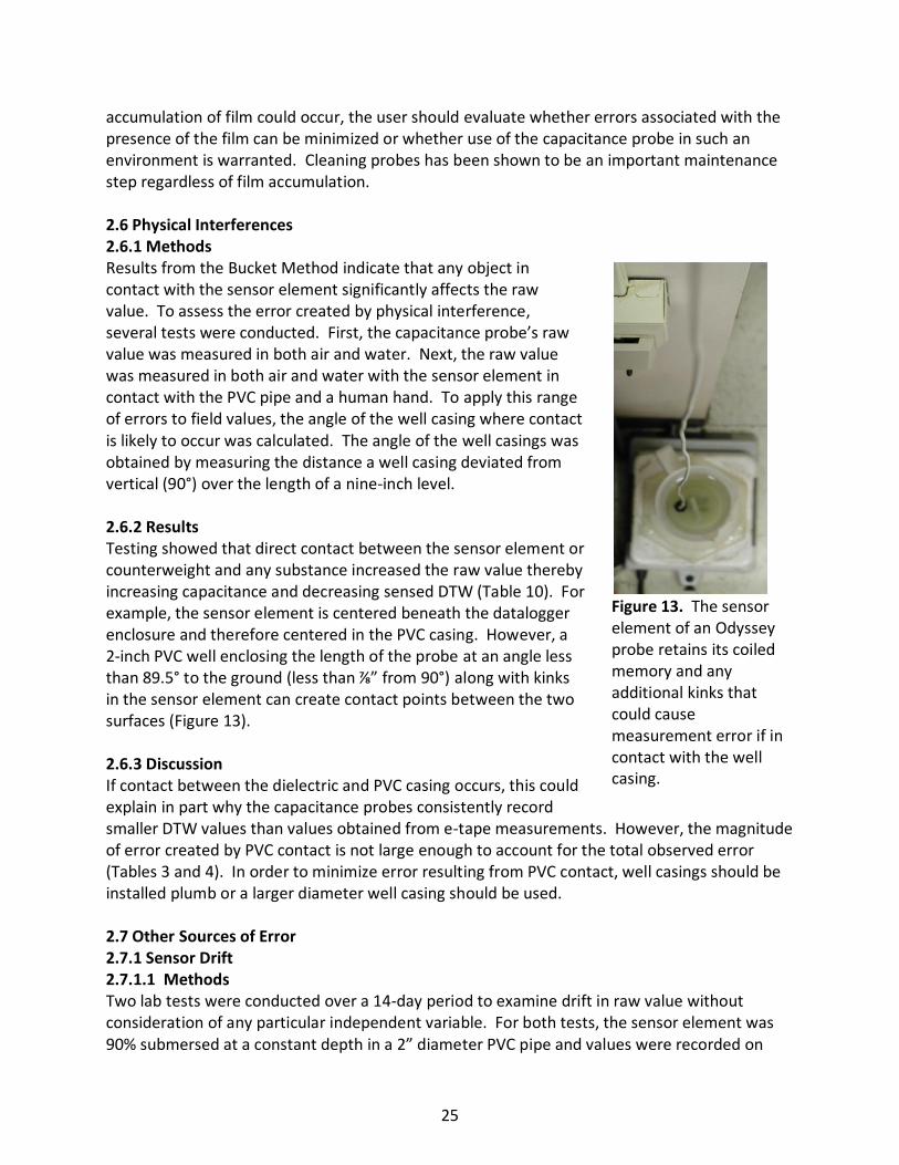
Figure 13. The sensor element of an Odyssey probe retains its coiled memory and any additional kinks that could cause measurement error if in contact with the well casing.

accumulation of film could occur, the user should evaluate whether errors associated with the presence of the film can be minimized or whether use of the capacitance probe in such an environment is warranted. Cleaning probes has been shown to be an important maintenance step regardless of film accumulation. 2.6 Physical Interferences 2.6.1 Methods Results from the Bucket Method indicate that any object in contact with the sensor element significantly affects the raw value. To assess the error created by physical interference, several tests were conducted. First, the capacitance probe’s raw value was measured in both air and water. Next, the raw value was measured in both air and water with the sensor element in contact with the PVC pipe and a human hand. To apply this range of errors to field values, the angle of the well casing where contact is likely to occur was calculated. The angle of the well casings was obtained by measuring the distance a well casing deviated from vertical (90°) over the length of a nine-inch level. 2.6.2 Results Testing showed that direct contact between the sensor element or counterweight and any substance increased the raw value thereby increasing capacitance and decreasing sensed DTW (Table 10). For example, the sensor element is centered beneath the datalogger enclosure and therefore centered in the PVC casing. However, a 2-inch PVC well enclosing the length of the probe at an angle less than 89.5° to the ground (less than ⅞” from 90°) along with kinks in the sensor element can create contact points between the two surfaces (Figure 13). 2.6.3 Discussion If contact between the dielectric and PVC casing occurs, this could explain in part why the capacitance probes consistently record smaller DTW values than values obtained from e-tape measurements. However, the magnitude of error created by PVC contact is not large enough to account for the total observed error (Tables 3 and 4). In order to minimize error resulting from PVC contact, well casings should be installed plumb or a larger diameter well casing should be used. 2.7 Other Sources of Error 2.7.1 Sensor Drift 2.7.1.1 Methods Two lab tests were conducted over a 14-day period to examine drift in raw value without consideration of any particular independent variable. For both tests, the sensor element was 90% submersed at a constant depth in a 2” diameter PVC pipe and values were recorded on

26

Table 9. Effect of physical contact between the sensor element and various materials. The DTW less than no-contact-DTW was approximated using a calibration slope of 2.

Contact between probe and various materials

Raw Value

Raw value greater than Raw value for no contact

DTW (mm) less than DTW for no contact

No Contact - Probe freely suspended in air 2112 0 0

Edge of counter weight contacting PVC 2123 9 5

Tip of counter weight and one point of sensor element on PVC 2135 23 22

One hand gripping counter weight 2131 19 10

One hand gripping element 2155 43 22

Two hands gripping element 2172 60 30

No Contact – Probe suspended in 765 μS/cm water 5307 0 0

Probe in 765 μS/cm water with an unknown number of contact points with PVC 5323 16 8

either 3-minute or 10-minute intervals. No test for drift in the probe’s internal clock was attempted. Measurement error was evaluated in order to indentify a negative or positive trending error since the probes’ deployment in June 2008. 2.7.1.2 Results For both trials, the observed decrease in sensed DTW was equal to the change in measured DTW due to evaporation. The results indicate that once the capacitance probe was stable, the probe did not drift and did not contribute error to the sensed DTW measurement. As of June 2009, no trend was observed in measurement error. 2.7.1.3 Discussion Frequent re-calibration of the probes would be necessary if sensor drift was observed; however, based on our laboratory tests and field observations, drift does not seem to be a significant factor affecting probe performance.

2.7.2 Experimental Error There are several sources of experimental error that may have been present during lab experiments that were not accounted for in DTW measurements. These sources of error include:

Raw values obtained using Odyssey software in trace mode (raw value every ≈2 seconds) were often unstable despite recording at a constant water level.

27

Instability of raw value output was often exacerbated at the extreme range of tested conditions.

Raw value readings were affected by whether the laptop computer was powered by battery or AC.

Accuracy of DTW measurements was limited both by e-tape precision (3.05 mm or 0.01 ft), although an attempt was made to measure within 1.52 mm (0.005 ft), and the 10 ml of water displaced by the weighted tape, which equates to a 5mm increase in water level inside a 2-in PVC pipe.

Physical contact between the PVC pipe and sensor element in lab calibrations could cause changes in the slope, offset, calibration curve and linearity of the Raw-DTW relationship. The sensor element was centered in the PVC pipe, but visually checking for physical contact was sometimes neglected. Movement of the pipe and sensor element during the calibration created errors.

Changes in chemistry of calibration water in uncovered buckets due to evaporation or atmospheric deposition over a two-week period.

3. Summary, Conclusions and Recommendations The Odyssey capacitance water level probe manufactured by Dataflow Systems Pty Ltd, Christchurch, New Zealand employs a commonly-applied relationship between electrical capacitance and water level. We found that water levels measured using the probe had a median measurement error that ranged from 11 to 288 mm using the bucket calibration method and 12 to 81 mm using the PVC pipe calibration method, per manufacturer’s suggested calibration and maintenance procedures. Tests conducted to date analyzing the effects of physical interferences, temperature, electrical conductivity, contact with the PVC casing, film, calibration method and calibration curve fitting on capacitance probe operation have revealed several of the most probable variables likely to affect sensed water level. Variables found to most significantly affect capacitance probe performance were: calibration method, variable water conductivity, and accumulation of film on the sensor element. Probes have poor accuracy in low conductivity water and we do not recommend their use below 4150 µS/cm. If used below 4150 µS/cm, we found that probes require a polynomial calibration in order to obtain a ± 5 mm accuracy, because the raw-DTW relationship becomes nonlinear as conductivity decreases. Possible additional error sources included a 5-mm rise in water level caused by e-tape displacement of water during manual e-tape measurements, and probe contact with PVC caused by an out-of-plumb casing. Based upon test results, we surmise that in order to reduce error and uncertainty by the greatest amount, the following should be used: frequent cleaning of capacitance probes, calibration in a PVC pipe using native groundwater, and frequent site visits to obtain manual water level measurements. We note that the latest version of the Odyssey manual does not contain instructions for using a bucket to calibrate a probe (Dataflow Systems 2008b).

28

References Dataflow Systems Pty Ltd. 2008a. PC Software and Technical Handbook for Odyssey Data Recorders. Christchurch, New Zealand, pp. 29-40. Received 22 Mar 2008. Dataflow Systems Pty Ltd. 2008b. Odyssey Water Level Capacitive Probe Handbook. Christchurch, New Zealand. Received 18 Dec 2008. Dataflow Systems Pty Ltd. Odyssey_productsview. 2008c. http://www.odysseydatarecording.com/odyssey_productsview.php?key=1, Accessed May 2008. Serway R.A., 2002. Jewett J.W., Principles of Physics: A Calculus-Based Text. 3rd ed. Brooks/Cole, United States.

http://www.odysseydatarecording.com/odyssey_productsview.php?key=1

29

Figure A1. Two-Point Fitting Error at Site 7.

-50

-40

-30

-20

-10

0

10

20

30

40

50

0 500 1000 1500 2000 2500

Two

-Po

int F

itti

ng

Erro

r (m

m)

Measured DTW (mm)

PVC, 3400 μS/cm, ≈20°C, 10/18/08

Figure A2. Two-Point Fitting Error at Site 20.

-50

-40

-30

-20

-10

0

10

20

30

40

50

0 500 1000 1500 2000 2500

Two

-Po

int F

itti

ng

Erro

r (m

m)

Measured DTW (mm)

PVC, 1575 µS/cm, 20°C, 10/11/08

PVC, 1575 µS/cm, 19°C, 10/11/08

Appendix A Calibration and Curve Fitting

evaluation of a capacitance water level recorder and calibration ... · the principle of...

Documents