evaluation and optimization of execution plans for...

IN DEGREE PROJECT COMPUTER SCIENCE AND ENGINEERING,SECOND CYCLE, 30 CREDITS

, STOCKHOLM SWEDEN 2016

Evaluation and Optimization of Execution Plans for Fixpoint Iterative Algorithms in Large-Scale Graph Processing

RICCARDO DIOMEDI

KTH ROYAL INSTITUTE OF TECHNOLOGYSCHOOL OF INFORMATION AND COMMUNICATION TECHNOLOGY

Abstract

In large-scale graph processing, a fixpoint iterative algo-rithm is a set of operations where iterative computation isthe core. The aim, in fact, is to perform repetitive opera-tions refining a set of parameter values, until a fixed pointis reached. To describe fixpoint iterative algorithms, tem-plate execution plans have been developed. In an iterativealgorithm an execution plan is a set of dataflow operatorsdescribing the way in which parameters have to be pro-cessed in order to implement such algorithms.

In the Bulk iterative execution plan all the parametersare recomputed for each iteration. Dependency plan cal-culates dependencies among vertices of a graph in order toiteratively update fewer parameters during each step. Todo that it performs an extra pre-processing phase. Thisphase, however, is a demanding task especially in the firstiterations where the amount of data is considerable.

We describe two methods in order to address the pre-processing step of the Dependency plan. The first one ex-ploits an optimizer which allows switching the plan duringruntime, based on a cost model. We develop three costmodels taking into account various features characterisingthe plan cost. The second method introduces optimizationsthat bypass the pre-processing phase. All the implementa-tions are based on caching parameters values and so theyare memory greedy.

The experiments show that, while alternative imple-mentation of Dependency plan does not give expected re-sults in terms of per-iteration time, cost models are ableto refine the existing basic cost model increasing accuracy.Furthermore, we demonstrate that switching plan duringruntime is a successful strategy to decrease the whole exe-cution time and improve performance.

Referat

Fixpunkt iterativa algoritmer är ett typiskt exempel påstorskalig bearbetning av grafer, där iterativa beräkning-ar är kärnan. Dess mål är att utföra upprepade operationeroch förbättra en uppsättning parametrars värde tills detatt en fast punkt nåtts. För att modellera fixpunkt itera-tiva algoritmer har exekveringsplansmallar utvecklats. Enexekveringsplan är en uppsättning av dataflödesoperatorersom beskriver sättet på vilket arametrarna

I den iterativa exekveringsplanen Bulk räknas alla pa-rametrar om för varje iteration. Exekveringsplanen Depen-dency beräknar beroenden mellan hörn i en graf för attiterativt uppdatera färre parametrar under varje steg. Föratt göra detta genomför den en extra förbehandlingsfas.Denna fas är dock krävande, i synnerhet under de förstaiterationerna där mängden data är betydande.

Vi beskriver två metoder för att adressera förbehand-lingssteget i exekveringsplanen Dependency. Den första ut-nyttjar en optimerare som tillåter exekveringsplansbyte un-der körning, baserat på en kostnadsmodell. Vi utvecklar trekostnadsmodeller som tar hänsyn till olika funktioner somkännetecknar planens kostnad. Den andra metoden intro-ducerar optimeringar som kringgår förbehandlingssteget.Alla implementationer baseras på cachning av parametrarsvärde samt minnesgirighet.

Experimenten visar att även om den alternativa imple-mentationen av Dependency-planen inte ger förväntade re-sultat sett till per-iteration tid, kan kostnadsmodeller förfi-na existerande grundkostnadsmodellens känslighet. Vidarevisar vi att ett planbyte under körning är en framgångs-rik strategi för att minska hela exekveringstiden samt ökarestandan.

Contents

List of Figures iii

List of Tables v

1 Introduction 11.1 Background . . . . . . . . . . . . . . . . . . . . . . . . . . . . . . . . 21.2 Notation . . . . . . . . . . . . . . . . . . . . . . . . . . . . . . . . . . 41.3 Problem Statement . . . . . . . . . . . . . . . . . . . . . . . . . . . . 41.4 Goal . . . . . . . . . . . . . . . . . . . . . . . . . . . . . . . . . . . . 61.5 Methodology . . . . . . . . . . . . . . . . . . . . . . . . . . . . . . . 71.6 Related Works . . . . . . . . . . . . . . . . . . . . . . . . . . . . . . 71.7 Outline . . . . . . . . . . . . . . . . . . . . . . . . . . . . . . . . . . 9

2 Theoretical Background 112.1 Apache Flink and Iterate operators . . . . . . . . . . . . . . . . . . . 112.2 Iterative Execution Plans . . . . . . . . . . . . . . . . . . . . . . . . 132.3 Connected Components in Apache Flink . . . . . . . . . . . . . . . . 16

3 Methods and Implementations 193.1 Cost Model . . . . . . . . . . . . . . . . . . . . . . . . . . . . . . . . 19

3.1.1 Legend . . . . . . . . . . . . . . . . . . . . . . . . . . . . . . 203.1.2 Basic Cost Model . . . . . . . . . . . . . . . . . . . . . . . . . 203.1.3 Cost Model with Shipping Strategies . . . . . . . . . . . . . . 213.1.4 Cost Model with Rebuilding Solution . . . . . . . . . . . . . 253.1.5 Cost Model with Cost Operation Discrimination . . . . . . . 26

3.2 Alternative Dependency Plans . . . . . . . . . . . . . . . . . . . . . 283.2.1 Alternative Dependency plan with cached neighbors’ values . 283.2.2 Alternative Dependency plan with cached neighbors . . . . . 293.2.3 Alternative Dependency with per-partition HashMap . . . . . 30

4 Results 354.1 Execution Environment Settings . . . . . . . . . . . . . . . . . . . . 354.2 Applications and Datasets . . . . . . . . . . . . . . . . . . . . . . . . 35

4.2.1 Connected Components (CC) . . . . . . . . . . . . . . . . . . 36

i

4.2.2 PageRank (PR) . . . . . . . . . . . . . . . . . . . . . . . . . . 364.2.3 Label Propagation (LP) . . . . . . . . . . . . . . . . . . . . . 364.2.4 Community Detection (CD) . . . . . . . . . . . . . . . . . . . 37

4.3 Tests Setting . . . . . . . . . . . . . . . . . . . . . . . . . . . . . . . 374.4 Tests Results . . . . . . . . . . . . . . . . . . . . . . . . . . . . . . . 38

4.4.1 Alternative Dependency plan tests . . . . . . . . . . . . . . . 384.4.2 Cost Model tests . . . . . . . . . . . . . . . . . . . . . . . . . 48

4.5 Discussion . . . . . . . . . . . . . . . . . . . . . . . . . . . . . . . . . 51

5 Conclusion and Future Work 53

Bibliography 55

List of Figures

1.1 Distributed Execution of Apache Flink . . . . . . . . . . . . . . . . . . . 41.2 Dependency Plan emphasizing the pre-processing phase . . . . . . . . . 51.3 Connected Components algorithm applied to the LiveJournal dataset

with three di�erent plans emphasizing the di�erent execution time amongBulk and Dependency . . . . . . . . . . . . . . . . . . . . . . . . . . . . 6

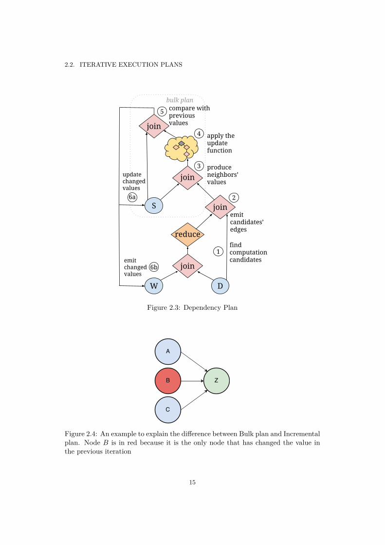
2.1 Flink’s Stack . . . . . . . . . . . . . . . . . . . . . . . . . . . . . . . . . 122.2 Bulk Plan . . . . . . . . . . . . . . . . . . . . . . . . . . . . . . . . . . . 142.3 Dependency Plan . . . . . . . . . . . . . . . . . . . . . . . . . . . . . . . 152.4 An example to explain the di�erence between Bulk plan and Incremental

plan. Node B is in red because it is the only node that has changed thevalue in the previous iteration . . . . . . . . . . . . . . . . . . . . . . . . 15

2.5 Incremental/Delta Plan . . . . . . . . . . . . . . . . . . . . . . . . . . . 162.6 Connected Components example . . . . . . . . . . . . . . . . . . . . . . 17

3.1 Cost Models Switching . . . . . . . . . . . . . . . . . . . . . . . . . . . . 223.2 Bulk plan with shipping strategies highlighted . . . . . . . . . . . . . . . 223.3 Plan-switching never occurs if D Ø 2S . . . . . . . . . . . . . . . . . . . 273.4 Node with cached values, only the changed in-neighbors send again their

values . . . . . . . . . . . . . . . . . . . . . . . . . . . . . . . . . . . . . 283.5 Comparison between the first implementation with the join and the sec-

ond with HashSet . . . . . . . . . . . . . . . . . . . . . . . . . . . . . . 303.6 Join - Reduce Dataflow and per-partition HashMap . . . . . . . . . . . 313.7 Example of Join - Reduce Dataflow with per-partition HashMap . . . . 32

4.1 Connected Components algorithm, LiveJournal . . . . . . . . . . . . . . 394.2 Community Detection algorithm, Orkut . . . . . . . . . . . . . . . . . . 404.3 Per-iteration time of updating hashmaps implementation on LiveJournal

dataset in Connected Components algorithm . . . . . . . . . . . . . . . 414.4 PageRank algorithm, LiveJournal . . . . . . . . . . . . . . . . . . . . . . 424.5 Label Propagation algorithm, LiveJournal . . . . . . . . . . . . . . . . . 434.6 Community Detection algorithm, LiveJournal . . . . . . . . . . . . . . . 444.7 Connected Components algorithm, Orkut . . . . . . . . . . . . . . . . . 454.8 PageRank algorithm, Orkut . . . . . . . . . . . . . . . . . . . . . . . . . 46

iii

4.9 Label Propagation algorithm, Orkut . . . . . . . . . . . . . . . . . . . . 474.11 Cost Models on LiveJournal dataset . . . . . . . . . . . . . . . . . . . . 484.10 Per-iteration time of PageRank algorithm . . . . . . . . . . . . . . . . . 494.12 Cost Models on Orkut dataset . . . . . . . . . . . . . . . . . . . . . . . 504.13 CC algorithm, Orkut dataset . . . . . . . . . . . . . . . . . . . . . . . . 51

List of Tables

4.1 Total iterations and crossing-point for LiveJournal dataset . . . . . . . . 494.2 Total iterations and crossing-point for Orkut dataset . . . . . . . . . . . 50

v

Glossary

CC Connected Components. 2, 6, 7, 13, 16, 17, 35, 36, 38, 41, 48, 50, 51

CD Community Detection. 35, 37, 38, 48, 50

DAG Directed Acyclic Graph. 3, 8, 33

HDFS Hadoop Distributed File System. 12, 13

JVM Java Virtual Machine. 3, 11

LP Label Propagation. 13, 35, 36, 48, 50

ML Machine Learning. 2

PR PageRank. 7, 13, 35, 36, 48, 51

UDF User-Defined Function. 2–4, 7, 8, 14, 16, 23, 24, 29, 32

vii

Chapter 1

Introduction

In graph theory, graphs are mathematical data structures used to model the rela-tions among objects. A graph is composed of vertices or nodes connected by edgesor arcs. Finding the shortest path to get from one city to another, ranking webpages, or even analyzing friendship links among users of social networks, are justsome use-cases easily modeled with graphs.

For decades, graph processing and analysis have been a useful tool not only incomputer science but also in other domains[1, 3]. Nowadays, with the growth ofgraphs’ size formed by billion or even trillion of nodes and edges, processing graph-structured data has become challenging. Furthermore, processing a large graphpresents some drawbacks such as poor locality of memory access, high data accessto computation ratio and irregular degree of parallelism during the execution[15].Large-scale graph processing is a term used to refer to processing a large amountof graph-structured data, too large to be processed in a single machine.

For this reason, there has been a rise in the use of large-scale graph systemsand general-purpose distributed systems recently, as both of them are able tohandle enormous graphs, deploying state-of-the-art distributed graph process-ing models[10, 9, 14].

In fact, it is common to partition and then distribute graph-structured dataamong multiple machines, instead of processing in a single one[15]. There aremany reasons for adopting such an approach. First of all, in some cases, if theamount of data is huge, they don’t fit within a single machine so it is preferable tosplit them across multiple machines. Furthermore, processing data in a distributedenvironment allows to exploit better process parallelism and, whether the degreeof parallelism of the program changes over the execution time, this environmentturns out to be more flexible[15]. Moreover, having multiple small commodity ma-chines is often cheaper than having just one with high memory capacity and a fastprocessor[15].

1

CHAPTER 1. INTRODUCTION

1.1 BackgroundIn the past years, high-level data-parallel frameworks have been largely exploited inorder to process and analyze data-intensive applications. One of the most famousand used for this purpose is MapReduce[4].

A type of data-intensive applications is the iterative applications which repeat-edly execute a set of operations. Typical examples are value propagation algo-rithms like Connected Components (CC) or Machine Learning (ML) algorithmslike Random Forest or Alternating Least Square. However, MapReduce frameworkperforms poorly with iterative applications because of the ine�ciency to performiterative operations[14]. Hence, programming abstractions like Grapx and Pregelhave been developed, which are able to handle these applications with large datasize[5, 16, 14].

An iteration-based algorithm is composed of several operations performed untila final condition is met. Well-known iterative-based algorithms are fixpoint iter-ative algorithms where input parameter values are refined in each iteration, andthe whole execution terminates when a convergence condition is met. The conver-gence condition in fixpoint iterative algorithms is often defined by the number ofconverged parameters. In particular, when all the parameters converge to a fixpoint,the execution terminates.

The parameters of a fixpoint iterative algorithm applied to a graph problem arethe vertices of the graph. In detail, in a fixpoint iterative graph algorithm, we definetwo input sets: the Solution set and Dependency set. The Solution set contains allthe nodes of a graph with related values, while the Dependency set contains all theedges of the graph. At the end of the execution, the Solution set indicates the finalsolution of the fixpoint algorithm, i.e. all the vertices with converged values. Weoften name the Solution set as Parameter set because it contains the parameters ofthe problem. In a fixpoint iterative graph algorithm, refining the parameter valuesmeans refining the value of each vertex until a fixpoint is reached.

In order to modify the value of the vertices and reach the fixpoint, an iterativeexecution plan has to be defined. An iterative execution plan is a set of dataflowoperators describing the way in which vertices have to be processed in order toimplement a fixpoint graph algorithm. Each plan is composed of two parts: aconstant part that is the same for each fixpoint algorithm, and a variable partdefined by the User-Defined Function (UDF), i.e. a function defined by the userthat implements the purpose of a fixpoint algorithm.

The execution plans di�er according to the operations involved into the dataflowand consequently, to the implemented logic. In this work, we always refer to fourspecific plans, deeply analyzed in Section 2.2. The four plans are:

• Bulk plan: the logic of this plan is to update all the nodes’ values in eachiteration.

• Dependency plan: it updates only those vertices that need to be recomputed,by filtering the Dependency set. Vertices that need to be recomputed are all

2

1.1. BACKGROUND

those that have not yet reached the fixed value.

• Incremental and Delta plans: these two plans have the same logic of Depen-dency plan but they can be applied with some constraints[11].

Incremental and Delta plans usually outperform the other two but they cannot beapplied with all the fixpoint graph algorithms because of the constraints. In thatcase, only Bulk and Dependency plan can be used. Since more than one plan can beused to solve a fixpoint iterative algorithm, choosing a suitable one is an essentialtask for both computational time and computational resources of the system.

The platform that has been used is Apache Flink[6], an open source platform fordistributed stream and batch data processing. It gives the possibility to manipulateand process data applying map, reduce, join and many other operators. The mostimportant feature that makes this platform suitable for fixpoint iterative algorithmsis that it natively supports iterative applications.

In general, input datasets are used to feed the platform and then transformed byoperators: in particular, the output of an operator is the input of another one. Theset of all operators is commonly represented as a Directed Acyclic Graph (DAG),that indicates the execution plan of the system.

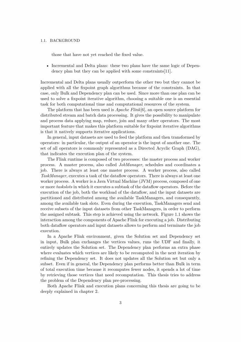
The Flink runtime is composed of two processes: the master process and workerprocess. A master process, also called JobManager, schedules and coordinates ajob. There is always at least one master process. A worker process, also calledTaskManager, executes a task of the dataflow operators. There is always at least oneworker process. A worker is a Java Virtual Machine (JVM) process, composed of oneor more taskslots in which it executes a subtask of the dataflow operators. Before theexecution of the job, both the workload of the dataflow, and the input datasets arepartitioned and distributed among the available TaskManagers, and consequently,among the available task slots. Even during the execution, TaskManagers send andreceive subsets of the input datasets from other TaskManagers, in order to performthe assigned subtask. This step is achieved using the network. Figure 1.1 shows theinteraction among the components of Apache Flink for executing a job. Distributingboth dataflow operators and input datasets allows to perform and terminate the jobexecution.

In a Apache Flink environment, given the Solution set and Dependency setin input, Bulk plan exchanges the vertices values, runs the UDF and finally, itentirely updates the Solution set. The Dependency plan performs an extra phasewhere evaluates which vertices are likely to be recomputed in the next iteration byrefining the Dependency set. It does not updates all the Solution set but only asubset. Even if in general, the Dependency plan performs better than Bulk in termof total execution time because it recomputes fewer nodes, it spends a lot of timeby retrieving those vertices that need recomputation. This thesis tries to addressthe problem of the Dependency plan pre-processing.

Both Apache Flink and execution plans concerning this thesis are going to bedeeply explained in chapter 2.

3


Figure 1.1: Distributed Execution of Apache Flink

1.2 NotationA fixpoint iterative graph problem can be defined by the following constructs:

• V ertex/Node set © Parameter set. Set of the nodes of a graph where eachnode is identified by a unique ID and a value related to the node itself. Arecord in this set is represented as following: (vertexID, vertexV alue). Wealso use another notation for the Parameter set that is, Solution set.

• Edge set © Dependency set. Set of all edges of a graph highlighting therelationships among nodes. Each entry is composed of a source ID, a targetID and possibly a value related to the edge. A record of this set is representedby: (sourceID, targetID, edgeV alue)

• UDF © step function. A function defined by the user and tailored for thespecific algorithm. It describes how a vertex value is updated according to itsneighbors’ values.

1.3 Problem StatementWhile Bulk and Dependency plans can always be used to implement a fixpointgraph algorithm, Incremental, and Delta plans cannot because of their constraintson the UDF. In detail, in order to apply either the Incremental or the Delta plan,the UDF of the fixpoint algorithm must be idempotent and weakly monotonic (seeSection 2.2).

4

1.3. PROBLEM STATEMENT

:

EXON�SODQ

'

6

MRLQ

MRLQ

MRLQ

MRLQ

UHGXFH

�

HPLW�FDQGLGDWHVÉ�HGJHV

�

SURGXFHQHLJKERUVÉ�YDOXHV

�

DSSO\�WKH�XSGDWH�IXQFWLRQ

�

FRPSDUH�ZLWKSUHYLRXVYDOXHV

�

XSGDWH�FKDQJHG�YDOXHV

�D

�EHPLW�FKDQJHG�YDOXHV

ILQG�FRPSXWDWLRQ�FDQGLGDWHV

Figure 1.2: Dependency Plan emphasizing the pre-processing phase

In order to update fewer nodes in each iteration, the Dependency plan performsan extra phase called pre-processing in which it calculates nodes that need to beupdated and filters the Dependency set. Since not all the nodes of a graph changevalue in an iteration, it is possible to consider in the computation only a smallernumber of nodes that need recomputation. The value of a vertex might not changesince the last iteration for two reasons:

• no one of its neighbor vertices has modified their value;

• the new value is equal to the old one.

While Bulk plan considers all the nodes and all the edges in the computation, De-pendency plan is able to calculate those nodes that need to be recomputed, and thusexcludes converged nodes from computation. However calculating those nodes needsadditional operations. For this reason, Dependency dataflow is composed of moreoperations than the Bulk plan. Even if in general, Dependency plan outperformsBulk because it recomputes fewer parameters, sometimes the number of parametersis so high that this plan spends a lot of time to perform these extra tasks. To sumup, in order to calculate fewer nodes at each iteration, the Dependency plan mustperform more operations than Bulk.

So, we can state that the pre-processing phase is a drawback for the Dependencyplan especially when the size of the datasets involved in the computation are high.Figure 1.2, taken from [11], highlights the demanding pre-processing phase thatrepresents the weak point of the Dependency plan.

5

Riccardo Diomedi


Figure 1.3: Connected Components algorithm applied to the LiveJournal datasetwith three di�erent plans emphasizing the di�erent execution time among Bulk andDependency

Other remarkable problems that we have to deal with even during the imple-mentation phase are both network and memory overhead. Exchanging data amongthe machines of the system, especially when data needs to be partitioned, requiresa lot of e�ort because network communication is such a bottleneck for the system.We face memory overhead instead when the amount of input data is really high. Inthat case, the main risk is that the system has no more available memory and so ithas to store some data on the disk decreasing the system performance.

Overall, the question is: considering all the constraints that we have to face inthis environment, is it possible to reduce the total execution time, especially of theDependency plan, and so increase the performance of the system?

1.4 GoalFigure 1.3, also taken from [11], shows the iteration time of three di�erent plans,applying CC algorithm on the LiveJournal dataset[22]: Bulk, Dependency, andIncremental plan. Without considering the Incremental plan, what stands out isthe clear di�erence in terms of time between Bulk and Dependency in the first fewiterations.

The goal of the thesis project is to reduce the total execution time of a fixpointalgorithm when Incremental and Delta plans cannot be used. In other words, re-

6

1.5. METHODOLOGY

ducing the execution time by using either Bulk or Dependency plans. We wantto accomplish the goal by either avoiding to execute Dependency plan in the firstiterations using instead the Bulk plan, or trying to bypass the pre-processing phaseof the Dependency exploiting some strategies. Overall, we want to push forward theperformance of the system decreasing the whole execution time and consequentlysave resources.

1.5 MethodologyRegarding the methods that we want to apply in order to reach our goal, a possiblestrategy would be to quantitatively evaluate the cost of both Bulk and Dependencyplans taking into account the main factors a�ecting the iteration execution timeand decide then which one to perform in the next iteration. Basically, the intentionis to study the cost factors for each plan and then develop a cost-based optimizerwhich is able to automatically select and switch plans. This method should lead toa more e�cient total execution time by avoiding redundant computations.

Furthermore, as the Dependency plan outperforms the Bulk from a certain iter-ation onward, another approach might be to modify the Dependency plan bypassingthe pre-processing phase. Successively, results coming both from alternative Depen-dency plan and the standard one are then formally and experimentally comparedin order to assess if a reduction of the iteration execution time can be achieved.

Using both methods and mixing the two strategies could head to the goal.

1.6 Related WorksExcluding the literature[11], which is the basis of this work, there are no worksdirectly linked to an in-depth study of execution plan cost for fixpoint iterativegraph algorithms in a distributed batch data processing environment.

Starting from literature[11], four execution plans for large-scale graphs process-ing are shown: Bulk plan, Dependency plan, Incremental plan and Delta plan.While the first two can be adopted in every case, the last two are applied underspecific constraints, explained in Section 2.2. The execution model and the maindi�erences between plans have been highlighted implementing some of the mostwell-known fixpoint iterative graph algorithms, such as PageRank (PR) and CC,and showing that the Incremental and Delta plan, whether they can be applied,outperform the other two.

Pregel is one of the most popular high-level frameworks for large-scale graphprocessing[16]. This framework consists of a sequence of iterations called superstepwhere, in parallel, vertices receive messages sent from in-neighbors in the previousstep, run a UDF and forward messages to the out-neighbors. In this literaturea vertex-centric approach is used, i.e. the focus is on the local computation ofthe vertex and is independent of other vertex computation. If a vertex does notreceive a message in a superstep, it is automatically disabled. A deactivated node

7


can be reactivated only if it receives a message from another node. The iterationterminates when all nodes are deactivated and there are no more messages in transit.Pregel implements the Incremental plan by default because only the nodes that havereceived at least one message from an in-neighbor are considered active.

The model of computation used in this literature and the one adopted in thethesis are similar. Abstractly, the message passing model of Pregel is a notablereference for our model of computation in which the nodes of the graph firstlyexchange values among them and then execute the UDF function.

Message passing among di�erent machines constitutes a large overhead. If forinstance, the sum of the values of the received messages is the important informationfor computation, then we can combine messages directed to a target node in a singleone before sending, in order to decrease the communication overhead. This taskis performed by combiners. Aggregators are another feature of this framework andmay be a valid reference for our work because they are able to perform statisticson the graph and evaluate the distribution. Aggregators are also implemented inApache Flink[6].

Several systems have been developed using Delta plan execution, a noteworthyone is REX[18]. REX is a good reference because it develops a system for recursivedelta-based data-centric computation. In this literature, the Delta plan is imple-mented through the user-defined annotations where delta, i.e. di�erence betweenthe last change and the old one, is seen as a tuple with annotation. An annotationtells the operator which operations such as inserting, deleting, replacement or UDF,have to be performed on that tuple. Operators keep unchanged nodes state andmodify records only according to the delta.

REX optimizer takes into account network, disk and CPU costs as well as di�er-ent interleaving of joins and UDF where predicates that are cheaper or discard morerecords should perform first. Furthermore, in deterministic functions, the constantparts should be cached in order to reuse data with lower overhead. Regarding therecursive computation, since it is composed of a base case and a recursive one, theoptimizer first estimates the base case cost and obtains the optimal plan for it, thenconsiders it as an input of the recursive case and retrieves again the optimal plan.This is repeated at each iteration considering the previous plan as an input andcosts are calculated accordingly. In the end, the optimal plan is chosen.

Literature [5] explains a method to integrate Bulk and Incremental iterationswith parallel dataflow. Parallel dataflow is a programming paradigm which modelsa program with a DAG of operators, a source, and a sink. This implementationimproves the exploitation of sparse computational dependencies present in manyiterative algorithms. Sparse Computational Dependencies means that, taking agraph as input, the change of a vertex a�ects its neighbors only.

While Bulk plan is equally implemented to the related work[11], the Incrementalone is developed di�erently, despite being conceptually similar. Further details ofall execution plans are showed in Section 2.2.

To implement an alternative Dependency execution plan, we were inspired bythe way this paper implements the Incremental execution plan.

8

1.7. OUTLINE

The optimizer estimates the cost of the iterative part and non-iterative part inorder to pick a plan. Since it is not possible to know a priori how many times we needto compute the iterative part, the optimizer chooses the iteration plan dependingon the cost of the first iteration. Moreover, a second optimization is cashing theconstant iteration parts. In other words, all the parts that remain constant can bestored in a hash table or B+ tree in such a way to avoid every time the overheadto redo it.

1.7 OutlineThe thesis starts o� with an overview of the theoretical background related to thetopic in Section 2. The theoretical background is then followed by Section 3 wherean in-depth analysis of di�erent implementation methods is shown with particularattention to the studied cost models. In Section 4 the experimental results of theimplemented methods are presented, followed by a discussion. Lastly, in Section 5a conclusion is drawn and future work are described.

9

Chapter 2

Theoretical Background

2.1 Apache Flink and Iterate operators"Apache Flink is an open source platform for distributed stream andbatch data processing. Flink’s core is a streaming dataflow engine thatprovides data distribution, communication, and fault tolerance for dis-tributed computations over data streams. Flink also builds batch pro-cessing on top of the streaming engine, overlaying native iteration sup-port, managed memory, and program optimization.[7]"

Born as an academic project named Stratopshere[2], Apache Flink platform isnow widely exploited for distributed big data analysis and processing. One of themost important features that makes it suitable for iterative application is its nativesupport for iterations. Similar platforms are Apache Hadoop[24], a framework thatallows for the distributed processing of large datasets across clusters of computersusing simple programming models such as MapReduce[4]; and Apache Spark[17],another engine for large-scale data processing.

Figure 2.1 is an overview of Flink’s stack[6]. The core of Flink is a DistributedStreaming Dataflow, on top of which there are two APIs both for batch and forstreaming processing, respectively: DataSet API and DataStream API. Once aFlink program is written employing all the operations that the platform provides,it is then parsed and a first rough plan is drawn. The first plan does not containany information regarding the strategy adopted by the system for partitioning thedatasets and the specific type of needed operations. This naive plan is then opti-mized by the Optimizer of the system. The purpose of the Optimizer is to evaluateall the transformations that need to be done on the input datasets and consequently,to choose the most appropriate type of operator for each operation, and the mostappropriate partitioning strategy for each operator.

Flink programs can be written either in Java or in Scala and then deployedin di�erent environments: in a Local environment, running a JVM, otherwise ei-ther in a Cluster environment like YARN[23] or in Cloud exploiting, for instance,OpenStack platform[20].

11

CHAPTER 2. THEORETICAL BACKGROUND

Figure 2.1: Flink’s Stack

Deepening in the implementation of a Flink program, an input dataset can becreated by loading a file from di�erent sources: either from a local file system orfrom a distributed file system like Hadoop Distributed File System (HDFS). Theinput datasets can be even created within a Flink program. According to the resultthat we want to retrieve and the algorithm that we implement, the datasets arethen manipulated and transformed by operators provided by Flink. Listing someof them, we have[8]:

• Map and FlatMap operator: it allows to map a dataset into another one, evenwith di�erent fields. An example might be to take a record composed by twointeger values, and return a di�erent record with just a single value that isthe sum of the previous two.

• Group By –> Aggregate operator: it allows to group a dataset on a given keyand then perform an aggregation operation such as: selecting the Max/Minand Sum.

• Group By –> Reduce operator: it allows to group a dataset on a given key andthen perform on each group a reduce function. The constraint of the Reduceis that if the input type is I also the output type must be I.

• Group By –> Combine operator: it allows to group a dataset on a given keyand then perform on each group a combine function. Here the type constraintof the Reduce is not considered.

12

2.2. ITERATIVE EXECUTION PLANS

• Distinct operator: it allows to eliminate duplicates within a single dataset.

• Project operator: it allows to eliminate one or more fields of a dataset.

• Join operator: it allows to literally join two or more datasets together andpotentially apply an operation on the intermediate result such as consideringonly some fields as the final result.

• coGroup operator: it jointly processes two or more datasets. The utility of thisfunction over the join is that the user can separately iterate over the elementsof both joined datasets.

Once the dataset is transformed, the relative result is returned via a sink thatmay be a raw file, a text file, a standard output like error stream or output stream,or a distributed file system like HDFS.

Apache Flink provides a useful tool in order to perform iterative algorithms:the iterative operator. In the iterative operator the user can define a step functionrepeatedly performed in each iteration until a convergence condition is reached.Two alternative iterative operators are provided: Iterate and Delta Iterate. In theIterate operator, the Solution set is entirely updated with the calculated partialsolution at the end of each iteration. In the Delta operator, not only the Solutionset but also a Working set is defined and filled with those parameters that havechanged their value according to the step function. Iteratively, while the Workingset is entirely updated with the new updated parameters, in the Solution set, onlythose parameters that changed their value are substituted.

The execution terminates when a convergence condition is fulfilled. Usually,the convergence condition is the maximum number of iterations. Flink also givesthe possibility to define a tailored convergence condition that it is verified beforestarting a new iteration. However, this is possible only in the Iterate operator.

The final result is represented by the last partial solution in the case of theIterate operator and by the solution set state after the last iteration in Delta Iterateoperator.

2.2 Iterative Execution PlansThere are four iterative execution plans analyzed in the literature [11]: Bulk Plan,Dependency Plan, Incremental Plan and Delta Plan. An execution plan is a set ofdataflow operators describing the way in which parameters have to be processed inorder to implement fixpoint iterative algorithms such as CC, PR, or Label Propa-gation (LP). In this section, we describe both the dataflow shaping each plan andthe main operating principles.

Starting from the Bulk, we can define this plan as the simplest one. Figure 2.2shows its mode of operation. The plan joins two input datasets: the Solution setS and the Dependency set D, in order to produce neighbors’ values and exchangethose values among the vertices. After joining, the intermediate result is then used

13


FRPSDUH�ZLWK�SUHYLRXV�YDOXHV

6 '

MRLQ

MRLQ

�

�

XSGDWHDOO�YDOXHV


�


�

Figure 2.2: Bulk Plan

to feed the UDF or step function that performs a specific task according to thepurpose of the algorithm. The last step is to compare the new partial solution withthe old one updating the Solution set with the new values. In fact, the most relevantfeature of this plan is that the Solution set is entirely updated at the end of eachiteration: so even those vertices that have not been modified are renewed.

The second plan under focus is the Dependency execution plan. The Dependencyplan can be seen as an optimization of the Bulk. In the Bulk plan, although thevalues of some vertices are not changed, all of them are updated anyway. In fact,all the vertices are updated even if their values are not changed. The value of avertex might not change since the last iteration for two reasons. Either no one ofits neighbor vertices has modified their value or the new value is equal to the oldone. Therefore, the Dependency plan avoids recomputing those vertices.

What stands out from Figure 2.3 is that the Dependency plan is a Bulk planwith a pre-processing phase at the bottom. The purpose of the pre-processing isto find candidates for recomputation, depending on the Working set: a subset ofthe Solution set containing updated vertices in the previous iteration. Doing thatthe Dependency set is shrunk by removing all those edges connected to alreadycomputed vertices. As a result, fewer vertices will be involved in the computation.Both Bulk and Dependency are the two plans that we have mainly studied in thisthesis work.

Regarding the Incremental plan and Delta plan, only the first one is shown andthen we introduce the minor di�erences with the second. The Incremental planis really similar to the Bulk but, instead of calculate neighbors’ values using theSolution set in the first join, it involves the Working set in order to perform thisoperation.

We can explain the result of substituting the Solution set with the Working setby using Figure 2.4. If we join the Solution set with the Dependency set, the result

14

2.2. ITERATIVE EXECUTION PLANS

:

EXON�SODQ

'

6

MRLQ

MRLQ

MRLQ

MRLQ

UHGXFH

�

HPLW�FDQGLGDWHVÉ�HGJHV

�


�


�

FRPSDUH�ZLWKSUHYLRXVYDOXHV

�


�D


ILQG�FRPSXWDWLRQ�FDQGLGDWHV

Figure 2.3: Dependency Plan

Figure 2.4: An example to explain the di�erence between Bulk plan and Incrementalplan. Node B is in red because it is the only node that has changed the value inthe previous iteration

15


':

6

MRLQ

MRLQ


�


�

FRPSDUH�ZLWK�SUHYLRXV�YDOXHV�


�D


Figure 2.5: Incremental/Delta Plan

is that, in the case in Figure 2.4, all the in-neighbors of node Z send their valuesto Z, even if only node B has changed the value. This is what happens in the Bulkplan. Note that node B is colored with red to indicate that it is the only node thathas changed the value in the previous iteration. In the Incremental plan instead,only B sends its value to Z. In this way, node Z will receive only a value from Bin the current iteration.

However, this plan has some constraints: the UDF that we apply must be idem-potent[26] and weakly monotonic[27]. Figure 2.5 illustrates the dataflow of this plan.The di�erence between Incremental and Delta plan is that while in the Incremental,the updated vertices send the total value to their neighbors, in Delta plan only thedelta, i.e. the di�erence between the new and the old value, has to be sent. As aconsequence, the amount of exchanged data is usually smaller.

2.3 Connected Components in Apache Flink

To give an idea of how Flink can implement a fixpoint iterative graph algorithm, weshow the implementation of the CC algorithm. The objective of this algorithm is tofind the number of Connected Components of a graph. A Connected Componentis a subgraph composed by all those nodes connected by a path. This goal can beaccomplished by scattering the initial value of each node in the graph until all haveconverged. The initial value of a node might be a random value or the ID number ofthe node itself. In many cases, the minimum value is propagated so each node hasto decide on it. Collecting the minimum flooded values, the connected componentsnumber can be finally obtained. Figure 2.6 shows the execution of this algorithmcomposed by two phases:

1. Active nodes of the graph send their values to their neighbors;

16

2.3. CONNECTED COMPONENTS IN APACHE FLINK

Figure 2.6: Connected Components example

2. Each vertex decides on a value according to the step function (in the figure,the minimum value).

With regard to the code, two dataset structures are firstly created: one forvertices and one for edges. DataSet is a Flink structure that models the set of itemsof the same type. The Tuple is a type of Flink Java API that specifies the itemfields. For the CC algorithm, the vertices Dataset is defined as follows:

DataSet<Tuple2<K, V>> v e r t i c e s ;

Each vertex item is composed by a key K and a value V that symbolizes respectively:the ID and the Connected Components value of the node.The edges Dataset instead is defined like:

DataSet<Tuple3<K, K, E>> edges ;

In this set, the first two fields are respectively the ID of source node and targetnode and this pair represents an edge, while the third one is the value associatedwith the edge. In the specific case of Connected Components, the third value is nullbecause the value of an edge is not involved in the process.

If we want to implement the algorithm using Bulk plan, we should define theIterate operator as follows:

I t e ra t iveDataSet <Tuple2<K, V>> i t e r a t i o n = v e r t i c e s . i t e r a t e (

maxIte rat ions ) ;

// . . .

// d e f i n e s t e p func t i on

// . . .

i t e r a t i o n . c loseWith ( parametersWithNewValues ) ;

The closeWith function of the Iterate operator represents the last operation wherethe Solution set is updated with a new partial solution previously calculated. Ev-erything defined within the operator is repeatedly performed until the convergence

17


condition is fulfilled. By default, the convergence condition is the maximum numberof iterations defined in the iterate function.

The first task that needs to be done is the exchange of the value among graphnodes. Vertices and edges set are then joined together to perform this task.DataSet<Tuple4<K, K, V, E>> parametersWithNeighborValues = i t e r a t i o n .

j o i n ( edges ) . where (0 ) . equalTo (0 ) . with (new ProjectStepFunct ionInput ( )

) ;

The result of the joined, called parametersWithNeighborValues, is then projectedin order to take into account only some fields. It can be seen as the set of valuesreceived by each single node of the graph. Next, step function is called and fed withthe intermediate result:DataSet<Tuple2<K, V>> parametersWithNewValues =

parametersWithNeighborValues . groupBy (0) . aggregate ( Aggregat ions .MIN,

2) . p r o j e c t (0 , 2) ;

The result of the step function is the vertices set with updated values. CloseWithfunction performs the last step to rebuilding the Solution set with the new computedvalue.

18

Chapter 3

Methods and Implementations

In order to solve the stated problem in Section 1.3 and accomplish the goal, we havedeveloped two methods. The first one determines the factors that a�ect the cost ofa plan in terms of time and builds a cost model that allows an optimizer to selecta plan with lower cost. This method requires an in-depth study of cost factors foreach iterative execution plan and the development of a cost-based optimizer thatautomatically decides the suitable plan. Actually, the plan-switching operation isperformed by imposing a convergence condition for the Bulk plan (see Section 2.2).In fact, since the Bulk always outperforms the Dependency in early iterations, theidea is to start to execute a job using Bulk and define a convergence condition whichallows the comparison between the two plans cost models. When the cost of theDependency becomes smaller than Bulk, then switch the plan.

The second method tries to optimize the Dependency plan bypassing the pre-processing phase. This phase is the heaviest part of the plan, especially when theamount of data is really high. A possible solution is to cache neighbors’ valueswithout the need to exchange them every time when it is not necessary. Even-tually, we formally and experimentally evaluate the alternative implementation ofDependency execution plan with the standard Dependency.

3.1 Cost ModelA cost model gathers the main features of a plan by defining a formula. Calculatingthe cost of a plan means then applying a formula that gives as output a numberindicating the value of the execution plan. This retrieved plan value is strictlyrelated to the total execution time of a single iteration of the plan itself. Thus, theidea is to calculate the cost of both Bulk and Dependency plan at the beginning ofeach iteration, and then choose at runtime which one has a lower cost.

We build the model in a modular way, i.e. we add as many terms in the formulaas the number of involved operations in the dataflow of the execution plan. Toevaluate the cost of an operation, we consider both the cost of the operator and thesize of the datasets used to perform that operation. Only the Dependency plan must

19

CHAPTER 3. METHODS AND IMPLEMENTATIONS

be recalculated because the cost of the Bulk plan never changes during iterations.The reason is that Bulk plan works with the same datasets and operations in eachiteration, so its cost model does not need to be recomputed every time. Moreover,what is important is not the real cost of a plan but rather understanding which ofthe two is the cheaper.

Starting from the basic cost model discussed in [11], we have studied factors thatmay a�ect the cost of a plan. The system gives di�erent performances dependingon the plan that we are running. Hence, changing the plan-switching point modifiesthe total execution time of the algorithm.

In the following part, we are going to highlight all the models, item by item,mainly focusing on advantages and drawbacks.

3.1.1 LegendShown below, a list of all the symbols that we use in the formulas of the cost models.

• Cj

: Join Cost

• Cr

: Reduce Cost

• cp

: Shipping Cost

• cb

: Rebuilding Cost

• S: Solution set

• D: Dependency set

• W : Working set, #updated nodes

• Z: Candidates set, #candidate nodes

• ⁄k

: #updatedNodes

Solutionset

, 0 Æ ⁄k

Æ 1

• µk

: #candidateNodes

Solutionset

, 0 Æ µk

Æ 1

3.1.2 Basic Cost ModelThe Basic Cost Model is described in the draft of [11]. This model approximatesthe cost of the two plans with the size of the inputs datasets. In fact, it is assumedthat the cost of an operation is independent of its type, and it only depends on thesize of the involved datasets. In addition, the computation cost of each operatorcan be considered irrelevant if compared to the network and memory overhead.

Considering only the size of the datasets, the cost of the Bulk plan is alwaysthe same over iterations, while, the cost of the Dependency changes because ofthe Working set and the Candidates set, i.e. the set containing re-computationcandidates. In fact, the Working set usually becomes smaller as iterations progressand so the cost of the Dependency plan accordingly decreases.

20

3.1. COST MODEL

We assume that at the k ≠ th iteration, the Working set contains ⁄k

ú S nodes,while Candidates set contains µ

k

ú S nodes. Since both the Working set and theCandidate set are subsets of the Solution set, ⁄

k

and µk

factors are between 0 and 1.The Candidates set is strongly related to the Working set because re-computationcandidates, i.e. all those nodes that are recomputed during the current iteration,are retrieved from the elements of the Working set.Following, the cost models of both plans:

BulkCost: Cj

(S + D) + Cr

D + Cj

2S = 3Cj

S + (Cj

+ Cr

)DDepCost: C

j

(⁄k

S +D)+Cr

⁄k

D +Cj

(D +µk

S)+Cj

(S +µk

D)+Cr

µk

D +Cj

(S +µ

k

S) = Cj

(⁄k

+ 2µk

+ 2)S + [Cj

(µk

+ 2) + Cr

(µk

+ ⁄k

)]D

The aim is to satisfy this formula:

DepCost Æ BulkCost

which means:

Cj

(⁄k

+ 2µk

+ 2)S + [Cj

(µk

+ 2) + Cr

(µk

+ ⁄k

)]D Æ 3Cj

S + (Cj

+ Cr

)D (3.1)

As already discussed, we assume Cj

= Cr

, and considering only the size of thedatasets, C

j

= Cr

= 1.The formula becomes:

(⁄k

+ 2µk

+ 2)(S + D) Æ 3S + 2D ∆ (⁄k

+ 2µk

)(S + D) Æ S

Another assumption made in this model is to consider ⁄k

equal to µk

, which meansto consider the size of the Working set equal to the size of the Candidates set.Applying ⁄

k

= µk

, the formula becomes:

3⁄k

(S + D) Æ S ∆ 3⁄k

Æ S

S + D(3.2)

Plot in Figure 3.1 displays the trend of the Bulk and Dependency costs respect to⁄

k

. The same plot shows the switching point between the two costs.

3.1.3 Cost Model with Shipping StrategiesThe next step is to consider the shipping strategies adopted by each plan. A shippingstrategy is how the platform decides to distribute one or more datasets across allthe parallel instances of the system in order to perform a distributed operation. In ascenario where the size of the datasets is extremely large, distributing the workloadand shipping data become key tasks. Regarding the cost of shipping, both the e�ortto partition the data and the overhead to distribute them need to be considered.

Figure 3.2 shows an example of how the system, specifically Apache Flink, selectsthe most suitable shipping strategies for the Bulk execution plan. Even if many

21


Figure 3.1: Cost Models Switching

Figure 3.2: Bulk plan with shipping strategies highlighted

shipping strategies can be used to partition data, in our specific case, only theforward strategy and hash partition have been used. The forward strategy indicatesthat a dataset does not need to be distributed because it is already partitionedacross the nodes, while hash partition exploits a hash function based on a key toperform this task.

According to the performed operation, the shipping strategy is then picked. Inour case, the two operations that influence the choice of the shipping strategies arethe join and the reduce operators.

In a distributed environment, the way we perform the join operation strongly de-pends on the considered datasets and, consequently, this a�ects the total cost. Fromliterature [21], the most appropriate types of join for parallelization are natural-join

22

3.1. COST MODEL

and equi-join.In order to perform a distributed join, the two datasets have to be partitioned on

the join attribute, i.e. the attribute on which datasets are going to be merged, thus,parallelizing the entire operation. Thanks to the partition result indeed, a singlenode is able to perform the local join in a subset of the input datasets, without theinconvenience of missing data.

Regarding the equi-join, there are three types of such operations, depending onhow the involved datasets are partitioned.

• Co-located join: both datasets are partitioned on the join key using a hashfunction. The cost only depends on the locally performed join.

• Directed join: only one of the two datasets is partitioned on the join at-tribute and therefore even the second dataset must be partitioned on thesame attribute. The cost of this operation is clearly higher than the previousone and is equal to the cost of partitioning the not-partitioned dataset, plusshipping the data over the network and finally the local cost of such operation.The cost of partitioning and shipping can be approximated to the number ofblocks forming the dataset.

• Repartition join: neither of the two datasets is partitioned on the joinattribute, so both must be partitioned. The cost is twice the partitioning andshipping since two datasets are involved, plus the local execution of the join.

Another possible solution to merge two datasets is the Broadcast join. One ofthe two datasets is already partitioned on the join attribute, but instead of runningthe partitioning of the other one, it is entirely sent to all nodes. In brief, the firstdataset is already partitioned on di�erent nodes, the second is sent to all. Thistechnique is often used when the size of one of the two datasets is much smallerthan the other.

Regarding the shipping strategy adopted to execute a reduce function, this de-pends both on how the dataset is distributed among nodes and on the specific typeof reduce operation. The reduce function involves just a dataset that could be ei-ther an input dataset or the intermediate result of another operation. Often, if thedataset needs to be partitioned, a first instance of the reduce function is locallyapplied. Then, the dataset is distributed and finally a second instance is applied.

An example is eliminating the duplicates in a dataset. In this case, the removalfunction is first applied before partitioning. The dataset is then partitioned anddistributed by the shipping strategy on a key likely to be the same of the reducefunction, and eventually the reduce function is applied again. Note that, performingthe reduce function before distributing data, decreases data tra�c over the network.For instance, the first reduce function of the Dependency plan operates in this way,removing duplicates of the intermediate result given by the join between Workingset and Dependency set.

The UDF is a reduce function di�erent from the first reduce of the Dependency,briefly explained in the sentence above. It is impossible to know a priori the shipping

23


strategy adopted by the system to execute the UDF. The reason why is that whilethe first reduce of the Dependency never changes from an algorithm to anotherbecause it is independent of it, the UDF is tailored to the algorithm itself and so itchanges every time. But, we do not need to know the exact value of the plan cost,rather which is the best moment to swap it whereby to decrease the entire executiontime of the program. Thus, the problem does not exist since the UDF is applied inthe same way both to Bulk and Dependency plans. In general, evaluating the costof a reduce function is taking into account the cost of partitioning, shipping, andlocal computation.

As in the Basic Cost Model, the cost of the shipping strategy has been weighedaccording to the size of the involved datasets. Taking as reference the book [21],the cost of partitioning and shipping is based on the size and number of blocksconstituting the dataset. Clearly, considering into the model the number of blocksof a dataset would be inappropriate because this value would change dependentlyfrom the hardware specification of the platform. For this reason, this value has beenapproximated with the size of the datasets. Starting from equation (3.1), Bulk plancost and Dependency plan cost become:

BulkCost: cp

S + cp

D + Cj

(S + D) + cp

D + Cr

D + cp

(2S) + Cj

2S = 3cp

S +2c

p

D + 3Cj

S + (Cj

+ Cr

)DDepCost: c

p

(⁄k

S) + cp

D + Cj

(⁄k

S + D) + cp

(⁄k

D) + Cr

⁄k

D + cp

D + cp

(µk

S) +C

j

(D + µk

S) + cp

S + cp

(µk

D) + Cj

(S + µk

D) + cp

(µk

D) + Cr

µk

D + cp

S + cp

(µk

S) +C

j

(S + µk

S) =c

p

[(⁄k

+ 2µk

+ 2)(S + D)] + Cj

(⁄k

+ 2µk

+ 2)S + [Cj

(µk

+ 2) + Cr

(µk

+ ⁄k

)]D

where cp

1 is the cost of the shipping strategy. In cp

both partitioning datasetand shipping over the network costs are included.As figure 3.2 displays, only the Dependency set is partitioned and shipped amongthe available nodes, and this is true also for Dependency plan. So both cost modelsturn into:

BulkCost: 2cp

D + 3Cj

S + (Cj

+ Cr

)DDepCost: c

p

(⁄k

+ 2µk

+ 2)D + Cj

(⁄k

+ 2µk

+ 2)S + [Cj

(µk

+ 2) + Cr

(µk

+ ⁄k

)]D

Again we want to know when:

DepCost Æ BulkCost

and so when:

cp

(⁄k

+ 2µk

)D + Cj

(⁄k

+ 2µk

)S + [Cj

(µk

+ 1) + Cr

(µk

+ ⁄k

)]D Æ Cj

S + Cr

D

Assuming Cj

= Cr

= 1 and even cp

= 1:

(⁄k

+ 2µk

)D + (⁄k

+ 2µk

)S + (µk

+ 1 + µk

+ ⁄k

)D Æ S + D ∆1We used lower case for shipping strategy cost and upper case for operator cost.

24

3.1. COST MODEL

(⁄k

+ 2µk

)S + (2⁄k

+ 4µk

)D Æ S ∆ (⁄k

+ 2µk

)(S + 2D) Æ S

and with ⁄k

= µk

finally we have:

3⁄k

Æ S

S + 2D

Nevertheless, the system optimizer caches the result of some operations withoutthe need to calculate it again. So, because of caching values, some of the terms re-lated to the shipping cost in the previous formula are redundant. Bearing in mindthis optimization, the cost models of both plans become:

BulkCost: cp

D + 3Cj

S + (Cj

+ Cr

)DDepCost: c

p

(⁄k

+ 2µk

)D + Cj

(⁄k

+ 2µk

+ 2)S + [Cj

(µk

+ 2) + Cr

(µk

+ ⁄k

)]D

Arguing again the same hypothesis, the final formula is:

(2D + S)(⁄k

+ 2µk

) Æ (S + D) ∆ (⁄k

+ 2µk

) Æ (S + D)S + 2D

Comparing this model with the Basic Cost Model (see formula (3.2)), it can benoticed that the Dependency plan su�ers from the shipping strategies more thanBulk. This is understandable because, in the pre-processing phase of Dependencyplan, many manipulations on datasets are performed, particularly on Dependencyset, and this certainly leads to a higher cost.

3.1.4 Cost Model with Rebuilding SolutionRebuilding the solution at the end of each iteration has been another executionstrategy taken into consideration during the study of the model. While for theBulk plan, at the end of each step, the Solution set must be rebuilt from scratchmodifying even those nodes that do not need recomputation, for Dependency, bothWorking set and Solution set are updated with a number of nodes that changesiteration by iteration. This number is always less or at most equal to the totalnumber of graph nodes.

Starting from equation (3.1) and using the term cb

2 to indicate the cost ofrebuilding solution, we have:

Cj

(⁄k

+2µk

+2)S +[Cj

(µk

+2)+Cr

(µk

+⁄k

)]D +2Wcb

Æ 3Cj

S +(Cj

+Cr

)D +Scb

(3.3)where W = ⁄

k+1S

Estimating the number of nodes used to rebuild the next Working set is a ratherdi�cult task because it would require the calculation of the whole step. For thisreason, we are going to consider W = ⁄

k+1S as W = ⁄k

S, aware that this is an2We used lower case for rebuilding cost and upper case for operator cost.

25


overestimation.Simplifying the formula assuming again C

j

= Cr

= 1, cb

= 1, and ⁄k

= µk

, itbecomes:

(3⁄k

+ 2µk

)S + (⁄k

+ 2µk

)D Æ 2S ∆ 5⁄k

S + 3⁄k

D Æ 2S

and so:⁄

k

Æ 2S

5S + 3D

Reflecting on the fact that the system faces a considerable work by reconstructingthe whole Solution set, another attempt has been to double only the cost of therebuilding, so having C

j

= Cr

= 1 and cb

= 2. Using equation (3.3) with thishypothesis, it becomes:

(5⁄k

+ 2µk

)S + (⁄k

+ 2µk

)D Æ 3S ∆ 7⁄k

S + 3⁄k

D Æ 3S

and so:⁄

k

Æ 3S

7S + 3D

NOTE: We tried to estimate W = ⁄k+1S, saving the size of W in the previous

iteration and then calculating the relation with the new one. Basically, we calculatethe relationship between the old and the new value in such a way:

” = Wk≠1

Wk

then we use this value in order to estimate the size of the next working set:

Wk+1 = W

k

”

3.1.5 Cost Model with Cost Operation DiscriminationRegardless of the specific operation type, the first idea has been to increase the costof the join, doubling it. We have made this test by keeping in mind that the costof a join is usually higher than other operations. Taking C

r

= 1 and Cj

= 2, theresult is the following:

BulkCost: 3D + 6SDepCost: D(⁄

k

+ 3µk

+ 4) + 2S(⁄k

+ 2µk

+ 2)

Thus:

D(⁄k

+3µk

+4)+2S(⁄k

+2µk

+2) Æ 3D+6S ∆ (⁄k

+3µk

)D+2S(⁄k

+2µk

) Æ 2S≠D

26

3.1. COST MODEL

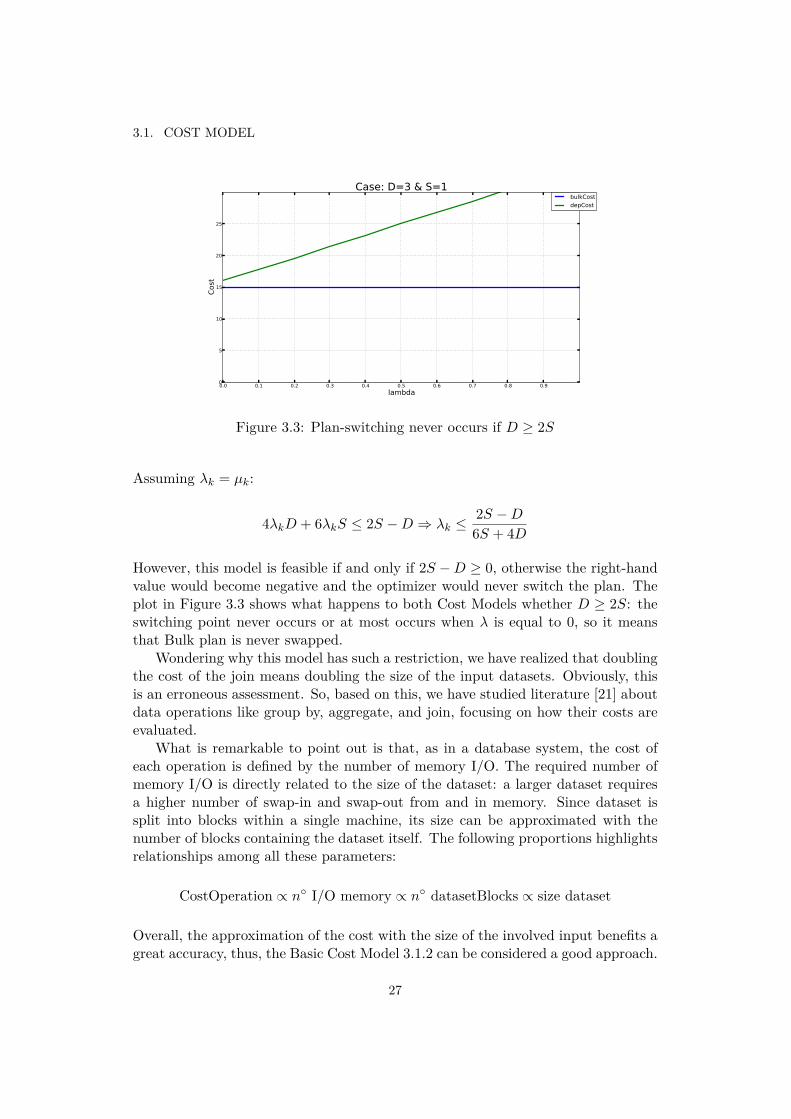
Figure 3.3: Plan-switching never occurs if D Ø 2S

Assuming ⁄k

= µk

:

4⁄k

D + 6⁄k

S Æ 2S ≠ D ∆ ⁄k

Æ 2S ≠ D

6S + 4D

However, this model is feasible if and only if 2S ≠ D Ø 0, otherwise the right-handvalue would become negative and the optimizer would never switch the plan. Theplot in Figure 3.3 shows what happens to both Cost Models whether D Ø 2S: theswitching point never occurs or at most occurs when ⁄ is equal to 0, so it meansthat Bulk plan is never swapped.

Wondering why this model has such a restriction, we have realized that doublingthe cost of the join means doubling the size of the input datasets. Obviously, thisis an erroneous assessment. So, based on this, we have studied literature [21] aboutdata operations like group by, aggregate, and join, focusing on how their costs areevaluated.

What is remarkable to point out is that, as in a database system, the cost ofeach operation is defined by the number of memory I/O. The required number ofmemory I/O is directly related to the size of the dataset: a larger dataset requiresa higher number of swap-in and swap-out from and in memory. Since dataset issplit into blocks within a single machine, its size can be approximated with thenumber of blocks containing the dataset itself. The following proportions highlightsrelationships among all these parameters:

CostOperation Ã n¶ I/O memory Ã n¶ datasetBlocks Ã size dataset

Overall, the approximation of the cost with the size of the involved input benefits agreat accuracy, thus, the Basic Cost Model 3.1.2 can be considered a good approach.

27


Figure 3.4: Node with cached values, only the changed in-neighbors send again theirvalues

3.2 Alternative Dependency PlansThe alternative method to the Cost Model introduces optimizations in order to by-pass the demanding pre-processing phase of the Dependency plan. In fact, the firsttwo join operations, involving Working set W , Candidates set Z and Dependencyset D, and the function used to remove duplicates, represent a critical part of thisplan, especially at the beginning where the sizes of the Working and Candidate setsare large because fewer nodes have reached the fixpoint value. But one of the mainfactors that decrease the performance of the system is the network communicationoverhead caused by the communication among nodes and the exchange of a greatamount of data.

We tried to tackle this problem presenting two memory greedy solutions thatavoid the massive usage of the network, and a third one where we exploit the wayin which parameters are partitioned among the task slots of the system, by cachingthem. In this case, monitoring the memory utilization is an important operation toperform.

3.2.1 Alternative Dependency plan with cached neighbors’ values

The logic of the Dependency plan (see Section 2.2) states that if at least one in-neighbor of a vertex changes value, all the in-neighbors of that vertex must sendtheir values. Focusing again on Figure 2.4, since node B has changed its value, evennode A and node C have to send again their values to Z. If none of the in-neighborsof node Z have been modified, it does not need to be recomputed. Therefore, theDependency execution plan asserts that if a vertex must be recomputed, it needsall the values of its in-neighbors in order to retrieve correct results at the end.

The first optimization caches the value of each in-neighbor for each node of thegraph so that unchanged nodes do not need to send the values. As Figure 3.4 shows,node Z has cached the values of its in-neighbors, and in each iteration, if one of theneighbors of Z is changed, it sends its new value. Note that the nodes that have not

28

3.2. ALTERNATIVE DEPENDENCY PLANS

changed their value during the last iteration do not send any value. From the samefigure, only B sends its value in the next iteration because it is the only node thathas been modified. Since the UDF is calculated based on the cached values, eachvertex must keep up-to-date the structure used to cache those values. Otherwise,the UDF is fed with erroneous data.

This solution has been realized adding in the Solution set an extra field repre-sented by a HashMap structure where in-neighbors’ values are stored. Thus, each en-try of the Solution set is composed of: (vertexID, vertexV alue, cachingHashMap).The HashMap of each node is composed of as many entries as the number of in-neighbors of that vertex, and each entry of the HashMap is the pair (key, value)where key and value are respectively the ID and the value of an in-neighbor.

However, this implementation su�ers from some drawbacks.First of all memory overhead: caching all those values leads to a higher memoryusage and the worst possible scenario may be the lack of main memory that forcesthe system to store some data on the disk. This operation decreases the systemperformance.

A second drawback is keeping up-to-date the HashMap of each node. In fact, ineach iteration, if a vertex sends the new value to its out-neighbors, all those verticeshave to modify the HashMap by updating the corresponding entry. For instance,in Figure 3.4 when node Z receives the new value from node B, it has to updatethe entry into the HashMap related to it. This is a required operation becausekeeping up-to-date the structure that caches the in-neighbors’ values is importantto correctly calculate the final result.

In addition to memory overhead, there is also the network overhead. TheHashMap in the Solution set constitutes a remarkable load for the system, par-ticularly when it has to rebuild the solution at the end of each iteration. In fact,the Solution set has to be sent over the network in order to perform this operationthat represents a bottleneck for the system performance.

3.2.2 Alternative Dependency plan with cached neighborsThe second optimization is not so di�erent from the execution plan of the stan-dard Dependency. In fact, instead of retrieving candidates joining the Working setwith the Dependency set, as usual, a HashSet has been used for each node con-taining all the out-neighbors and retrieve candidates through it. Like the previousimplementation, the HashSet has been put as an extra field in the Solution set.

Figure 3.5 shows the first part of the Dependency plan before and after the op-timization. With the new implementation, the join can be replaced with a FlatMapfunction in which the HashSet of each node of the Working set is iterated.

Actually, this optimization is already made by the system optimizer and so theremight not be so many di�erences between this solution and the optimized standardDependency plan. Moreover, this solution is also penalized from network overheaddue to the need to move the Solution set over the network as explained in Section3.2.1.

29


Figure 3.5: Comparison between the first implementation with the join and thesecond with HashSet

3.2.3 Alternative Dependency with per-partition HashMap

The concept is the same of the optimization shown in Section 3.2.1, i.e. caching thevalues of the in-neighbors of each vertex, but it has been implemented in a di�erentway. In fact, instead of instantiating the HashMap in the Solution set, we put thisstructure in each parallel instance of the system.

This solution executes the same dataflow operations of the Incremental plan,but it implements the same logic of the Dependency execution plan. Figure 3.6highlights the mode of operation.

Regarding the logical execution plan, the first operation is a join that allowsretrieving the parameters’ values, merging the Working and the Dependency sets.Abstractly, this operation may be seen as a message passing phase where onlythose parameters that are changed in the last iteration, send their value to theout-neighbors.

The second operation is a reduce function applied on the intermediate resultof the join, grouping on the ID field of the parameters. In the reduce function,neighbors’ values are cached in a HashMap data structure. In fact, a Hashmapfor each parallel instance of the system is instantiated and filled during the firstiteration, and each entry of this data structure is made by the parameter ID and itsneighbors’ values. Then, thanks to the partition strategy, the values for a specificvertex always end up in the same partition/instance of the system.

30


Figure 3.6: Join - Reduce Dataflow and per-partition HashMap

Since in this case the Hashmap is not defined for each vertex but for eachpartition, it has a slightly di�erent structure compared to the solution in Section3.2.1. Each entry of the HashMap instantiated in each partition is composed of a keyrepresenting the ID of a vertex and a value that is another HashMap containing thevalues of the in-neighbors of this vertex. The reason to have two nested HashMapis because, in each partition, we need to store the in-neighbors’ values of more thanone vertex.

Giving an example of how the reduce function operates, we consider a graphcomposed of four nodes: 1, 2, 3 and 4, like in Figure 3.7. Since the system relieson two instances, the execution of the program can be parallelized by a factor of 2.Moreover, while nodes 1 and 2 are processed within the first partition and so theneighbors’ values of these nodes are cached in the HashMap of this partition, theneighbors’ values of nodes 3 and 4 are cached in the second one. If a vertex changesvalue, the first join emits as many records as the number of its out-neighbors. So, iffor instance, node 3 has changed its value and node 1, 2 and 4 are its out-neighbors,only two records end up in the first partition. These records represent the twomessages sent by node 3 to node 1 and 2. The HashMaps of both partitions arethen updated with newly received records in order to always keep it up-to-date.

31


Figure 3.7: Example of Join - Reduce Dataflow with per-partition HashMap

Starting from the values cached into the Hashmap, the UDF is then locallyperformed to the reduce function and eventually a comparison between the newand the old values of the parameters is made by a second join in order to retrievethe updated vertices. Finally, the Solution set and the Working set are updated.

This optimization reduces the network overhead exploiting the computationalcapacity of each single machine.

Alternative Dependency with per-partition HashMap Cost Model

After implementing the optimized Dependency plan of Section 3.2.3, we evaluateand design a Cost Model for it as we have done in Section 3.1. In this case, however,we have to consider the memory overhead and computational complexity of the planoperations. In fact, while in the execution plans showed in [11] the datasets aremainly manipulated by distributed operations, in this solution, local computationis largely exploited. Instead of performing the step function through distributedjoin and aggregate operators, for instance, this is performed using data structuresfrom the Collection library such as Map, List and so on. As a result, this solutionis memory and computationally expensive, since a single machine has to locallyexecute many operations.

The following Cost Model has been designed without considering the memory,

32


assuming so an infinite quantity of it. In other words, only the logical plan has beentaken into account, i.e. the DAG of the plan. Thus, we have:

AltDepCost : (⁄k

S + D)Cj

+ ⁄k

DCr

+ (µk

S + S)Cj

(3.4)

Clearly, this cost model is a rough approximation of the real plan cost, but it is animportant starting point for more accurate analysis.

Now, as we did before, we want to know when:

AltDepCost Æ BulkCost

thus, when:

(⁄k

S + D)Cj

+ ⁄k

DCr

+ (µk

S + S)Cj

Æ 3Cj

S + (Cj

+ Cr

)D

Always assuming that Cj

= Cr

= 1 and ⁄k

= µk

, eventually we have:

⁄k

(2S + D) Æ 2S + D ∆ ⁄k

Æ 1

According to this model then, Bulk plan should never be used because ⁄k

isnever greater than 1. This makes sense because alternative Dependency has thesame logical plan of the Incremental and, as we have explained in Section 2.2,Incremental plan always outperforms Bulk.

However, with this dataflow the part related to the memory usage has not beenconsidered, i.e. all the operations in reduce function where hashmap is involved.Therefore, also the e�ort to handle this data structure has to be taken into accounttracking the time of that specific part of the implementation.

Nevertheless, measuring time complexity of operations performed within thereduce function is not an easy task. Trying to figure it out and evaluate such com-plexity with numbers might lead to a complex and unfeasible model. In addition,calculating such complex model might be ine�ective and can waste a lot of time.So the goal is trying to keep it as simple as possible.

Because of that, an extra term representing the memory usage is added, withoutthe need to calculate it with a complex formula. The value of this term is likelyhigh in the first iterations, but then, decrementing the data to deal with, it becomessmaller. The formula (3.4) therefore, becomes:

AltDepCost: (⁄k

S + D)Cj

+ ⁄k

DCr

+ (µk

S + S)Cj

+ mk

where with mk

we indicate the cost of caching operations at k ≠ th iteration.However, estimating such term and understanding how it behaves according to

other factors is not easy. For sure it is influenced by the size of the datasets and theavailable memory of the system. Hence, it is complicated to value this parameterindependently from the hardware. In fact, the more available memory you have,the more the alternative Dependency plan should outperform.

33

Chapter 4

Results

4.1 Execution Environment Settings

We have used two machines: sky2 (master and slave) and sky4 (slave) consisting of12 cores and 46 GB of memory each. The tests have been run in an environmentwith 16 CPUs and 72 GB of main memory in total. Each machine runs LinuxUbuntu 14.04.3 LTS and has 1.8.0 66 version Java(TM) SE Runtime Environmentinstalled.

A distributed file system has been deployed as well. In particular, 2.7.2 versionHadoop HDFS has been installed on both nodes: while in sky2 (master and slave)both namenode and datanode run, in sky4 (slave) only the datanode runs.

4.2 Applications and Datasets

By using our implementation, we have tested four fixpoint iterative algorithms:CC, PR, LP and Community Detection (CD). These four algorithms are going tobe explained the following subsection. (see subsections 4.2.1, 4.2.2, 4.2.3, 4.2.4)While the first two algorithms can be executed faster with Incremental and Deltaplan respectively, the last two do not, because they do not satisfy the constraintsof Incremental and Delta plan explained in Section 2.2.

For each of such algorithms, we have used Bulk, Dependency, and alternativeDependency plan. Furthermore, the input datasets for the tests have been takenboth from Stanford Network Analysis Project (SNAP)[22] and from Koblenz Net-work Collection[12], and are:

• LiveJournal: dataset with around 4 million nodes and 34 million edges.

• Orkut: dataset with 3 million nodes and 117 million edges.

35

CHAPTER 4. RESULTS

4.2.1 Connected Components (CC)CC algorithm aims to find the Connected Components of an undirected graph inwhich any pairs of vertices of a Connected Component are connected by a path.This result might be accomplished by flooding the graph with the initial valueof each vertex and then decide on the minimum value. In the end, the numberof di�erent minimum values represents the number of Connected Components ofthat graph. Thus, in each iteration, a vertex sends its value to the out-neighborsand meanwhile receives values from its in-neighbors. It then chooses the minimumamong all the received numbers and its own. When no vertex changes value, thealgorithm terminates.

4.2.2 PageRank (PR)PR is an iterative algorithm used to rank web pages according to the number ofreferences[19]. At the beginning, each vertex is initialized with a fixed value. Ineach iteration, a vertex receives neighbors’ values and it then applies the followingformula:

Pr

(y) = (1 ≠ d) + d(Nÿ

i=1

Pr

(xi

)C(x

i

) )

where:

• Pr

(y): PageRank of the studied page y.

• d: dump factor that is usually equal to 0.15.

• Pr

(xi

): PageRank of i-th page.

• C(xi

): number of links of i-th page.

PageRank of page y is determined by the sum of the ratio between the PageRankand the number of links of pages x

i

.At the end of the iteration, if the value of the page has changed for a delta

higher than a threshold, then the vertex/page remains active.

4.2.3 Label Propagation (LP)In LP algorithm, a graph has to unanimously decide on a label with the highestfrequency in order to find communities[28].

At the beginning, each node of a graph picks one label in a finite set of labels.In each iteration, a vertex gathers the labels of its neighbors and counts the numberof each one. Then it selects that with the highest frequency. In the case of a draw,i.e. two labels with the same highest number, a vertex chooses the label with thehigher value since labels are represented by numbers.

36

4.3. TESTS SETTING

4.2.4 Community Detection (CD)The goal of CD is to detect nodes communities within a graph based on labelmechanism[13].

At the beginning, while each node is initialized with a tuple of values representingrespectively the label of that node and its score, each edge is initialized with arandomly selected weight. Note that we initialize the edges with random valuesbecause our input graphs have no weights. In each iteration, a vertex gathers tuplesof its neighbors and according to the neighbor’s label score and the edge weight,it calculates a new score for each received label. After selecting the label with thehighest score, it then filters the previously received tuples with this label. In otherwords, among all the neighbors with label equal to the newly computed one, thevertex selects that with the highest score. If the new label of a vertex is equal to theprevious one, the score is updated with the selected higher neighbor’s score label,otherwise, the new label is adopted and its corresponding score is decreased with anumber depending on a fixed number and the number of iterations. Note that, thefixed number must be specified at the beginning of the algorithm and is equal to0.5 by default. The use of the delta value becomes very important in the algorithmbecause it tends to prevent the formation of monster community, thereby increasingthe reliability and the e�ciency of the algorithm[13].

4.3 Tests SettingTwo batches of tests have been run: the first to test the alternative implementationof Dependency plan, while the second to test Cost Models.

Regarding the first batch of tests, we have decided to test only the AlternativeDependency plan with per-partition HashMap (see Section 3.2.3), because the othersolutions waste a lot of time in rebuilding the solution due to the presence in theSolution set of the HashMap or HashSet. In addition, it is useless to execute thesolution explained in Section 3.2.2 because it is actually an optimization of theDependency plan already made by the Optimizer of the system. The aim anywayis to analyze the behavior of the alternative implementation of Dependency planwith respect to both Bulk plan and standard Dependency plan. In particular, whatwe want to find out is the per-iteration execution time for each execution plan. Todo that, we have tested every execution plan: Bulk, Dependency, and alternativeDependency, three times for each of the implemented algorithms. So overall, sincewe have four di�erent algorithms, we run 36 tests. All these tests have been run inorder to have as reliable results as possible.

Regarding the batch test of the Cost Model, the aim is to understand whetherconsidering more features such as the Rebuilding Solution, might bring better resultsin terms of total execution time. The body of this test is to run for each involveddataset and for each implemented algorithm, both Basic Cost Model and Cost Modelwith Rebuilding Solution, three times. We have decided to run Basic Cost Modeland Cost Model with Rebuilding Solution because the Basic one tends to switch

37

CHAPTER 4. RESULTS

plan from Bulk to Dependency later than the exact switching point. Since CostModel with Rebuilding Solution tends to penalize more Bulk and thus performsmore iterations with Dependency plan, as explained in Sections 3.1.3 and 3.1.4, itmight give better result in term of time.

There is, however, another possible batch test that could be done, i.e. testinga custom Cost Model where, instead of swapping Bulk plan with the standard De-pendency, using the alternative Dependency plan of Section 3.2.3. In fact, what weexpect is that the alternative plan should perform better especially in the last iter-ations because it processes fewer data. Nevertheless, alternative Dependency planalways performs worse than Dependency and sometimes even than Bulk consideringthe whole execution time.

However, before running this specific test, we need to verify whether and whenthe alternative Dependency plan outperforms either Dependency or Bulk plan.

4.4 Tests Results

4.4.1 Alternative Dependency plan tests

We have analyzed alternative Dependency plan together with Bulk and standardDependency on LiveJournal and Orkut datasets.

Despite, we have had good expectations from this implementation, it has notgiven however valuable results. In fact, we have thought that after the demandingwork at the beginning, it might result better than other plans. In addition, mineddata have highlighted a really weird behavior of the implementation itself. Thus,we have run some tests in order to debug it.

Figure 4.1a and figure 4.2a show the per-iteration execution time of Bulk (bulk),Dependency (dep) and alternative Dependency (dep_inc), in CD algorithm appliedto LiveJournal dataset and in CC algorithm applied to Orkut dataset. The alterna-tive Dependency tends to remarkably fluctuate between two values, from iterationto iteration.

As Figures 4.2b and 4.2a illustrate, the per-iteration time execution trend ofDependency plan, after slightly rising in iteration 14 and 15, it then starts to dropat iteration 15. Likewise, the number of updated elements, experienced a decreaseuntil iteration 10, it then goes up around iteration 14 and finally drops again.In particular, decreasing the number of elements, the per-iteration execution timesimilarly decreases. This is a clear evidence that the method that we have used tomeasure time is reliable and almost precise.

Trying to give a rational explanation of such strange results, we have started totest the implementation, debugging it. Following we are going to list all the debugthat we have made in order to solve this problem.

1. Since our implementation is memory greedy and easily susceptible from mem-ory usage, we have made sure that no one else was using the machine.

38

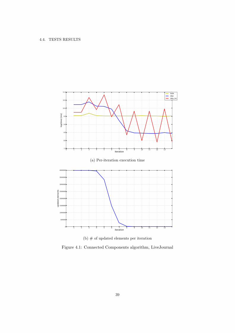
4.4. TESTS RESULTS

(a) Per-iteration execution time

(b) # of updated elements per iteration

Figure 4.1: Connected Components algorithm, LiveJournal

39

CHAPTER 4. RESULTS



Figure 4.2: Community Detection algorithm, Orkut

40

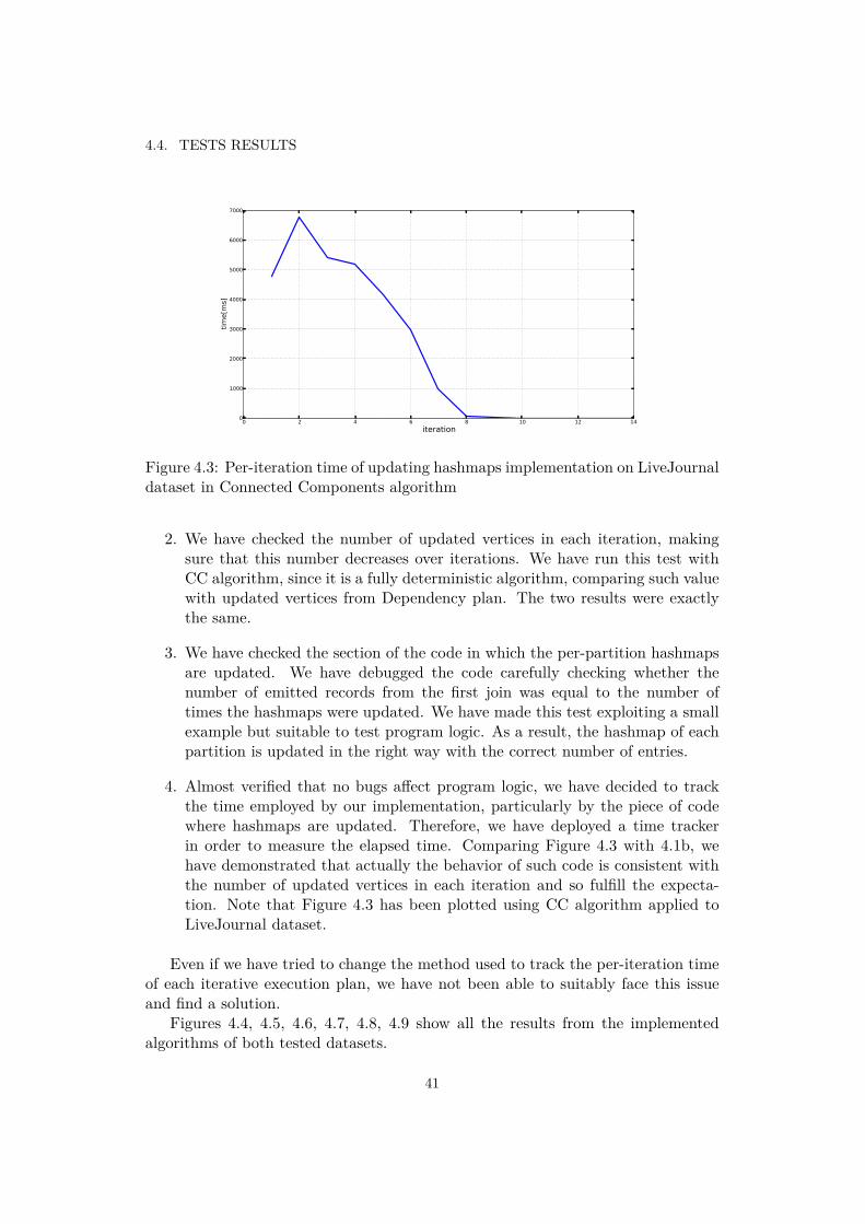
4.4. TESTS RESULTS

Figure 4.3: Per-iteration time of updating hashmaps implementation on LiveJournaldataset in Connected Components algorithm

2. We have checked the number of updated vertices in each iteration, makingsure that this number decreases over iterations. We have run this test withCC algorithm, since it is a fully deterministic algorithm, comparing such valuewith updated vertices from Dependency plan. The two results were exactlythe same.

3. We have checked the section of the code in which the per-partition hashmapsare updated. We have debugged the code carefully checking whether thenumber of emitted records from the first join was equal to the number oftimes the hashmaps were updated. We have made this test exploiting a smallexample but suitable to test program logic. As a result, the hashmap of eachpartition is updated in the right way with the correct number of entries.

4. Almost verified that no bugs a�ect program logic, we have decided to trackthe time employed by our implementation, particularly by the piece of codewhere hashmaps are updated. Therefore, we have deployed a time trackerin order to measure the elapsed time. Comparing Figure 4.3 with 4.1b, wehave demonstrated that actually the behavior of such code is consistent withthe number of updated vertices in each iteration and so fulfill the expecta-tion. Note that Figure 4.3 has been plotted using CC algorithm applied toLiveJournal dataset.

Even if we have tried to change the method used to track the per-iteration timeof each iterative execution plan, we have not been able to suitably face this issueand find a solution.

Figures 4.4, 4.5, 4.6, 4.7, 4.8, 4.9 show all the results from the implementedalgorithms of both tested datasets.

41

CHAPTER 4. RESULTS



Figure 4.4: PageRank algorithm, LiveJournal

42

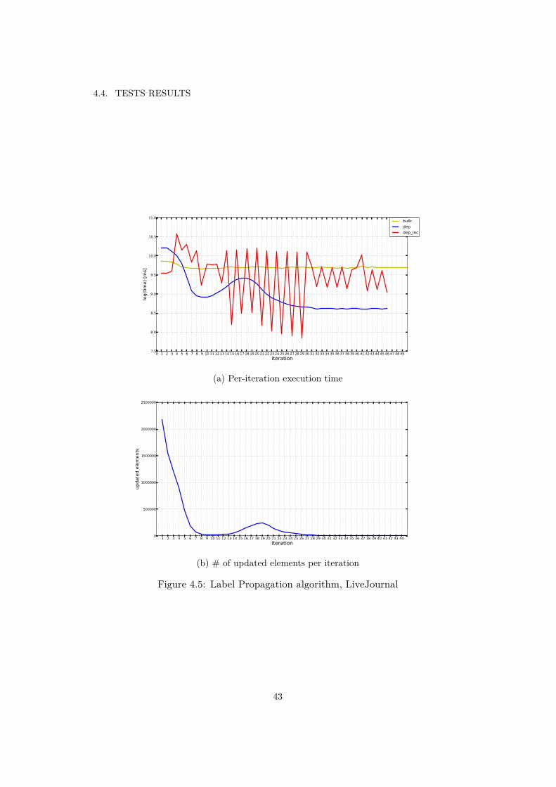
4.4. TESTS RESULTS



Figure 4.5: Label Propagation algorithm, LiveJournal

43

CHAPTER 4. RESULTS



Figure 4.6: Community Detection algorithm, LiveJournal

44

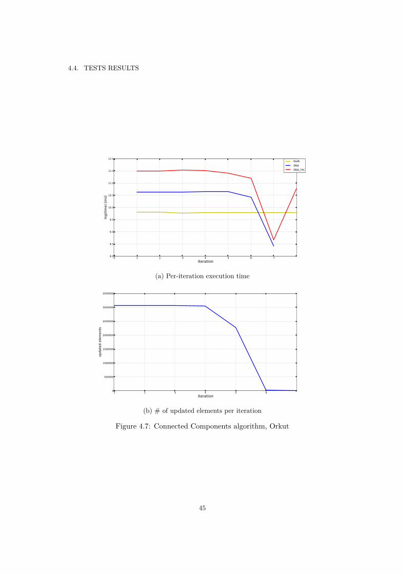
4.4. TESTS RESULTS



Figure 4.7: Connected Components algorithm, Orkut

45

CHAPTER 4. RESULTS



Figure 4.8: PageRank algorithm, Orkut

46

4.4. TESTS RESULTS



Figure 4.9: Label Propagation algorithm, Orkut

47

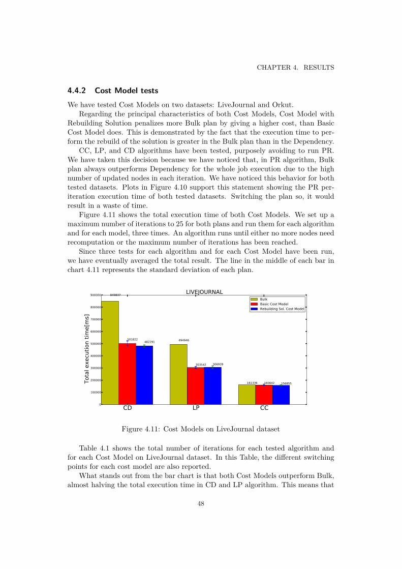
CHAPTER 4. RESULTS

4.4.2 Cost Model testsWe have tested Cost Models on two datasets: LiveJournal and Orkut.

Regarding the principal characteristics of both Cost Models, Cost Model withRebuilding Solution penalizes more Bulk plan by giving a higher cost, than BasicCost Model does. This is demonstrated by the fact that the execution time to per-form the rebuild of the solution is greater in the Bulk plan than in the Dependency.

CC, LP, and CD algorithms have been tested, purposely avoiding to run PR.We have taken this decision because we have noticed that, in PR algorithm, Bulkplan always outperforms Dependency for the whole job execution due to the highnumber of updated nodes in each iteration. We have noticed this behavior for bothtested datasets. Plots in Figure 4.10 support this statement showing the PR per-iteration execution time of both tested datasets. Switching the plan so, it wouldresult in a waste of time.

Figure 4.11 shows the total execution time of both Cost Models. We set up amaximum number of iterations to 25 for both plans and run them for each algorithmand for each model, three times. An algorithm runs until either no more nodes needrecomputation or the maximum number of iterations has been reached.

Since three tests for each algorithm and for each Cost Model have been run,we have eventually averaged the total result. The line in the middle of each bar inchart 4.11 represents the standard deviation of each plan.

Figure 4.11: Cost Models on LiveJournal dataset

Table 4.1 shows the total number of iterations for each tested algorithm andfor each Cost Model on LiveJournal dataset. In this Table, the di�erent switchingpoints for each cost model are also reported.

What stands out from the bar chart is that both Cost Models outperform Bulk,almost halving the total execution time in CD and LP algorithm. This means that

48

4.4. TESTS RESULTS

(a) LiveJournal

(b) Orkut

Figure 4.10: Per-iteration time of PageRank algorithm

LiveJournal CC LP CDTot. It. Switch-It Tot. It. Switch-It Tot. It. Switch-It

Basic C.M. 14 8 32 12 36 11C.M. with R.B. 14 8 36 10 36 10

Table 4.1: Total iterations and crossing-point for LiveJournal dataset

49

CHAPTER 4. RESULTS

Orkut CC LP CDTot. It. Switch-It Tot. It. Switch-It Tot. It. Switch-It

Basic C.M. 7 no 21 15 19 17C.M. with R.B. 7 6 20 14 19 17

Table 4.2: Total iterations and crossing-point for Orkut dataset

switching plans results in better performance and so it saves time.Except for LP, where the two Cost Models have performed a di�erent number

of iterations, both in CC and in CD, Cost Model with Rebuilding Solution havebrought a slight improvement.

Regarding CC algorithm, since both models switch the plans in the same itera-tion, we can consider the total execution times essentially equal.

The reason for such di�erence in LP is likely due to the comparison instructionssuch as choosing the maximum or minimum between two values. In that case, if thecomparing values are equal, it happens that di�erent runs provide di�erent results.This a�ects the total number of iterations and thus the total execution time of thejob. Nevertheless, the benefit of both Cost Models in LP algorithm is remarkable.

Figure 4.12: Cost Models on Orkut dataset

Bar chart 4.12 displays the execution time of Bulk plan and both Cost Modelson Orkut dataset.

With this dataset, Cost Model with Rebuilding Solution performs slightly worsethan Basic one. This is likely due to the number of dependencies within the Orkutgraph. In this situation, Dependency plan performs worse than Bulk because of thedemanding pre-processing phase, so it is more beneficial to execute more iterationsusing Bulk plan rather than Dependency.

50

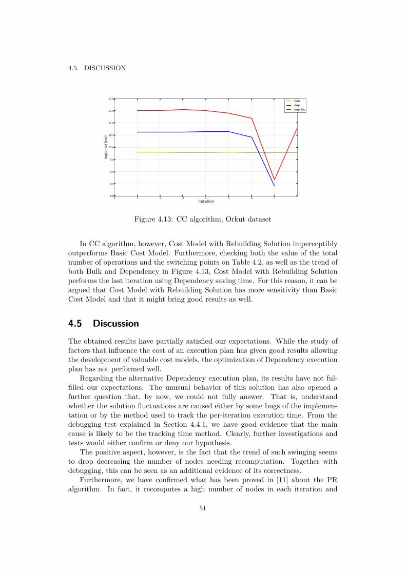
4.5. DISCUSSION

Figure 4.13: CC algorithm, Orkut dataset

In CC algorithm, however, Cost Model with Rebuilding Solution imperceptiblyoutperforms Basic Cost Model. Furthermore, checking both the value of the totalnumber of operations and the switching points on Table 4.2, as well as the trend ofboth Bulk and Dependency in Figure 4.13, Cost Model with Rebuilding Solutionperforms the last iteration using Dependency saving time. For this reason, it can beargued that Cost Model with Rebuilding Solution has more sensitivity than BasicCost Model and that it might bring good results as well.

4.5 DiscussionThe obtained results have partially satisfied our expectations. While the study offactors that influence the cost of an execution plan has given good results allowingthe development of valuable cost models, the optimization of Dependency executionplan has not performed well.

Regarding the alternative Dependency execution plan, its results have not ful-filled our expectations. The unusual behavior of this solution has also opened afurther question that, by now, we could not fully answer. That is, understandwhether the solution fluctuations are caused either by some bugs of the implemen-tation or by the method used to track the per-iteration execution time. From thedebugging test explained in Section 4.4.1, we have good evidence that the maincause is likely to be the tracking time method. Clearly, further investigations andtests would either confirm or deny our hypothesis.

The positive aspect, however, is the fact that the trend of such swinging seemsto drop decreasing the number of nodes needing recomputation. Together withdebugging, this can be seen as an additional evidence of its correctness.

Furthermore, we have confirmed what has been proved in [11] about the PRalgorithm. In fact, it recomputes a high number of nodes in each iteration and

51

CHAPTER 4. RESULTS

therefore it tends to not converge. For this reason, using a plan di�erent fromBulk always gives worse results. Such reasoning can hold without considering bothIncremental and Delta plan.

In the other hand, the study of di�erent Cost Models has revealed interesting as-pects about iterative execution plans cost. First of all, we have verified the accuracyand reliability of Basic Cost Model through an in-depth study of distributive oper-ations like join, group by and so on. Secondly, we have shown that some physicalfeatures, such as Rebuilding Solution, refine Basic Cost Model giving more sensi-tivity. Indeed, the detailed study has been helpful in order to understand how thesystem behaves according to such features and how they a�ect the whole executiontime of a plan.

52

Chapter 5

Conclusion and Future Work

In this work, we have talked about large-scale graph processing and fixpoint iterativealgorithms, explaining both the purpose and the way they work.

After briefly explaining the platform that we have used, we have shown anoverview of the already implemented plans, highlighting both advantages and dis-advantages of each of them.

We have claimed the problem that a�ects Dependency plan and then describedtwo methods in order to solve it. The first one is to study and develop a cost modelin order to evaluate both Bulk and Dependency and then choose during runtime thecheapest plan. The other one is to optimize standard Dependency plan bypassingthe heavy pre-processing phase.

We have finally run two batches of tests trying to bring to light fundamentalaspects of our solution in relation with the others. Even if we have retrieved un-expected results, we have given a contribution to fixpoint iterative algorithms byincreasing the knowledge and verifying, for instance, the correctness of Basic CostModel.

Regarding the future work, a helpful one is deeply analyzing the alternativeDependency plan solution, understanding which are the real factors a�ecting its be-havior. In our opinion, since the execution is partitioned and distributed among ma-chines, tracking the time is not a simple task and sometimes time tracking methoddoes not give accurate results. So, evaluating it might be a starting point.

Then, another future work might be studying the term in Section 3.2.3 related tothe caching operation. In particular, understand how this term behaves according toother memory factors, such as the size of the involved graph. Certainly, it results tobe useful if and only if we demonstrate that optimized Dependency plan outperformsstandard Dependency after some iterations.

Furthermore, we would like to analyze the relationship between ⁄k

and µk

ac-cording to di�erent graphs with di�erent features like cluster coe�cient, etc. We aresure that retrieving the correct number for both ⁄

k

and µk

leads to a more accurateevaluation of the already implemented cost models. For instance, two graphs withthe same number of vertices, but di�erent edges, they have a remarkable di�erence

53

CHAPTER 5. CONCLUSION AND FUTURE WORK

on the number of dependencies and so on the ⁄k

/µk

relationship.Further work may be to exploit other methodologies and data structures in order

to cache neighbors, developing then a di�erent Dependency execution plan. Forexample, BloomFilter [25] can be used in order to estimate the number of candidates.

54

Bibliography

[1] Tero Aittokallio and Benno Schwikowski. Graph-based methods for analysingnetworks in cell biology. Briefings in bioinformatics, 7(3):243–255, 2006.

[2] Alexander Alexandrov, Rico Bergmann, Stephan Ewen, Johann-ChristophFreytag, Fabian Hueske, Arvid Heise, Odej Kao, Marcus Leich, Ulf Leser,Volker Markl, et al. The stratosphere platform for big data analytics. TheVLDB Journal, 23(6):939–964, 2014.

[3] Alexandru T Balaban. Applications of graph theory in chemistry. Journal ofchemical information and computer sciences, 25(3):334–343, 1985.

[4] Je�rey Dean and Sanjay Ghemawat. Mapreduce: simplified data processingon large clusters. Communications of the ACM, 51(1):107–113, 2008.

[5] Stephan Ewen, Kostas Tzoumas, Moritz Kaufmann, and Volker Markl.Spinning fast iterative data flows. Proceedings of the VLDB Endowment,5(11):1268–1279, 2012.

[6] The Apache Software Foundation. Apache Flink an open source platform fordistributed stream and batch data processing., 2014-2015. [Online; accessed15-June-2016].

[7] The Apache Software Foundation. Apache Flink overview, 2014-2015. [Online;accessed 15-June-2016].

[8] The Apache Software Foundation. Dataset transformations, 2014-2015. [On-line; accessed 15-June-2016].

[9] Joseph E Gonzalez, Yucheng Low, Haijie Gu, Danny Bickson, and CarlosGuestrin. Powergraph: Distributed graph-parallel computation on naturalgraphs. In Presented as part of the 10th USENIX Symposium on OperatingSystems Design and Implementation (OSDI 12), pages 17–30, 2012.

[10] Joseph E Gonzalez, Reynold S Xin, Ankur Dave, Daniel Crankshaw, Michael JFranklin, and Ion Stoica. Graphx: Graph processing in a distributed dataflowframework. In 11th USENIX Symposium on Operating Systems Design andImplementation (OSDI 14), pages 599–613, 2014.

55

BIBLIOGRAPHY

[11] Vasiliki Kalavri, Stephan Ewen, Kostas Tzoumas, Vladimir Vlassov, VolkerMarkl, and Seif Haridi. Asymmetry in large-scale graph analysis, explained.In Proceedings of Workshop on GRAph Data management Experiences andSystems, pages 1–7. ACM, 2014.

[12] UniversitÃ¤t Koblenz Landau. The koblenz network collection. http:

//konect.uni-koblenz.de/. Accessed: 2016-05.

[13] Ian XY Leung, Pan Hui, Pietro Lio, and Jon Crowcroft. Towards real-timecommunity detection in large networks. Physical Review E, 79(6):066107, 2009.

[14] Yucheng Low, Danny Bickson, Joseph Gonzalez, Carlos Guestrin, Aapo Kyrola,and Joseph M Hellerstein. Distributed graphlab: a framework for machinelearning and data mining in the cloud. Proceedings of the VLDB Endowment,5(8):716–727, 2012.

[15] Andrew Lumsdaine, Douglas Gregor, Bruce Hendrickson, and Jonathan Berry.Challenges in parallel graph processing. Parallel Processing Letters, 17(01):5–20, 2007.

[16] Grzegorz Malewicz, Matthew H Austern, Aart JC Bik, James C Dehnert, IlanHorn, Naty Leiser, and Grzegorz Czajkowski. Pregel: a system for large-scalegraph processing. In Proceedings of the 2010 ACM SIGMOD InternationalConference on Management of data, pages 135–146. ACM, 2010.

[17] Xiangrui Meng, Joseph Bradley, Burak Yavuz, Evan Sparks, ShivaramVenkataraman, Davies Liu, Jeremy Freeman, DB Tsai, Manish Amde, SeanOwen, et al. Mllib: Machine learning in apache spark. arXiv preprintarXiv:1505.06807, 2015.

[18] Svilen R Mihaylov, Zachary G Ives, and Sudipto Guha. Rex: recursive,delta-based data-centric computation. Proceedings of the VLDB Endowment,5(11):1280–1291, 2012.

[19] Lawrence Page, Sergey Brin, Rajeev Motwani, and Terry Winograd. The pager-ank citation ranking: bringing order to the web. 1999.

[20] Omar Sefraoui, Mohammed Aissaoui, and Mohsine Eleuldj. Openstack: to-ward an open-source solution for cloud computing. International Journal ofComputer Applications, 55(3), 2012.

[21] Je�rey D Ullman and J Widom. Database systems: The complete book, 2000.

[22] Stanford University. Stanford large network dataset collection. http://snap.

stanford.edu/data/. Accessed: 2016-05.

56

http://konect.uni-koblenz.de/

http://konect.uni-koblenz.de/

http://snap.stanford.edu/data/

http://snap.stanford.edu/data/

BIBLIOGRAPHY

[23] Vinod Kumar Vavilapalli, Arun C Murthy, Chris Douglas, Sharad Agarwal,Mahadev Konar, Robert Evans, Thomas Graves, Jason Lowe, Hitesh Shah,Siddharth Seth, et al. Apache hadoop yarn: Yet another resource negotiator.In Proceedings of the 4th annual Symposium on Cloud Computing, page 5.ACM, 2013.

[24] Tom White. Hadoop: The definitive guide. " O’Reilly Media, Inc.", 2012.

[25] Wikipedia. Bloom filter — wikipedia, the free encyclopedia, 2016. [Online;accessed 15-June-2016].

[26] Wikipedia. Idempotence — wikipedia, the free encyclopedia, 2016. [Online;accessed 16-June-2016].

[27] Wikipedia. Monotonic function — wikipedia, the free encyclopedia, 2016. [On-line; accessed 16-June-2016].

[28] Xiaojin Zhu and Zoubin Ghahramani. Learning from labeled and unlabeleddata with label propagation. Technical report, Citeseer, 2002.

57

TRITA ICT-EX-2016:64

www.kth.se

evaluation and optimization of execution plans for...

Documents