evaluating the representation of precipitation in the ... · pdf fileobserved reflectivity of...
TRANSCRIPT

Evaluating the representation of precipitation in the COSMO model for Belgium
Tim Böhmea, Nicole van Lipziga, Laurent Delobbeb, Axel Seifert c
a Physical and regional geography group, Katholieke Universiteit Leuven, Belgium (KUL)
b Royal Meteorological Institute of Belgium (KMI)
C Deutscher Wetterdienst (DWD)
COSMO user seminar 2009 – Langen – 10 March 2009

Introduction Model setup Observations Results Outlook
QUEST-B: Focus on BelgiumThis presentation:Can the radar observations help to show a model progress from 3-21 to 4-3?
Preliminary results of three case studiesCOSMO user seminar 2009 – Langen – 10 March 2009
QUEST (Quantitative Evaluation of Regional Precipitation Forecast Using Multi-Dimensional Remote Sensing Observations)
Team (Susanne Crewell):- Institute for Geophysics and Meteorology, Universität zu Köln- Institute for Space Sciences, Freie Universität Berlin- Institute of Atmospheric Physics, DLR- Physical and Regional Geography Research Group, KU Leuven- Deutscher Wetterdienst, DWD- Meteorological Institute, Universität Hamburg

Region of interest:
COSMO user seminar 2009 – Langen – 10 March 2009
Introduction Model setup Observations Results Outlook

Topography of region of interest:
Topographical height in m:800 m0 m 300 m
COSMO user seminar 2009 – Langen – 10 March 2009
Introduction Model setup Observations Results Outlook

Atmospheric model• COSMO-DE model (Δx = 2.8 km), forcing with COSMO-EU• version 4-3, version 3-21 (on basis of 4-3)• in case studies comparison to changes in
gscp-routine and postprocessingchanges: (version 3-21 in brackets)- Intercept parameter for snow (equation of Field, 2005):
isnow_n0temp = 2 (0)- Factor in the terminal velocity for snow:
zv0s = 20.0 (4.90)zv1s = 0.50 (0.25)
- Formfactor in the mass-size relation of snow particles:zams = 0.069 (0.038)
- Change in parameter for sticking effect zeff = max. 0.2 (0.5)
COSMO user seminar 2009 – Langen – 10 March 2009
Introduction Model setup Observations Results Outlook

Atmospheric model COSMO 4-3:
Parts of the hydrological cycle in the model, which are affected by changes:
COSMO user seminar 2009 – Langen – 10 March 2009
Formfactor of mass-size relation of snow particles
Factor in the terminal velocity for snow
Intercept parameter using temperature-dependent moment relations (eq. Field et al. 2005)
Rain Snow
Precipitation and evapotranspiration at ground level
Cloud ice
Cloud water
Water vapour
Parameter for sticking effect
sedimentation
Conversion rates qi, qs, qg
Introduction Model setup Observations Results Outlook

C-band Doppler Radar (f = 5.6 GHz, λ = 5.4 cm)- Scans at 10 elevation angles each 15 minutes
(0.5 – 17.5°)- Horizontal resolution is 500 m in range and 1°
in azimuth- Use of volume data and Pseudo CAPPI data
- Actual 2 radars in Belgium: Wideumont (KMI)Zaventem (Belgo Control)
Satellite data (MSG, MODIS, CLOUDSAT)GPS dataSynoptical weather stations
Comparison to observations
COSMO user seminar 2009 – Langen – 10 March 2009
Introduction Model setup Observations Results Outlook

Kick-Off-Treffen PQP – Bonn – 10 / 11 April 2008
Introduction Model setup Observations Results Outlook

Radar data: Volume data and Pseudo CAPPI data
Volume data: 3D data-set from all radar beam datamaximum value in the column
Pseudo CAPPI data: Pseudo Constant Altitude Plan-Position Indicator product
COSMO user seminar 2009 – Langen – 10 March 2009
Volume data Pseudo CAPPI data
2006: W W + Z
2007: W + Z
NOW:
Introduction Model setup Observations Results Outlook

Radar data: Volume data and Pseudo CAPPI data
Volume data: 3D data-set from all radar beam datamaximum value in the column
Pseudo CAPPI data: Pseudo Constant Altitude Plan-Position Indicator product
COSMO user seminar 2009 – Langen – 10 March 2009
Volume data Pseudo CAPPI data
2006: W + Z W + Z
2007: W + Z W + Z
SOON:
Introduction Model setup Observations Results Outlook

Pseudo CAPPI::
COSMO user seminar 2009 – Langen – 10 March 2009
Radar beam of different elevations
Pseudo CAPPI represents reflectivity values at a given altitude above sea level(interpolating between reflectivity data from different elevations)
Radar of Wideumont: Pseudo CAPPI height = 1500 m
Introduction Model setup Observations Results Outlook

COSMO user seminar 2009 – Langen – 10 March 2009
Comparison Radar volume data (column maximum) and CAPPI data:
180 km radius
3 %
Introduction Model setup Observations Results Outlook
CAPPI data / 0.83
CAPPI data
Volume data(column maximum)
Histogram of the reflectivity distribution in dBZ classes
Total Z > 0 dBZ: 65,2% for volume data53,7% for CAPPI data

Stratiform precipitation case
23/11/2006
2 Convective cases
22/06/2007 23/06/2007
Case studies I:
COSMO user seminar 2009 – Langen – 10 March 2009
Introduction Model setup Observations Results Outlook

Case studies II: 23/11/2006
COSMO user seminar 2009 – Langen – 10 March 2009
In the morning:passing of a warm front
In the afternoon:passing of a cold front
500 hPa12 UTC
00 UTC
Introduction Model setup Observations Results Outlook

Case studies II: 23/11/2006
Observed reflectivity of warm front 04-07 UTC and cold front 12-15 UTC (radar CAPPI):
COSMO user seminar 2009 – Langen – 10 March 2009
warm front
cold front
04 UTC 05 UTC 06 UTC 07 UTC
12 UTC 13 UTC 14 UTC 15 UTC
Introduction Model setup Observations Results Outlook

Case studies II: 23/11/2006
Modelled reflectivity of the warm front 04-07 UTC and cold front 12-15 UTC (4-3):
COSMO user seminar 2009 – Langen – 10 March 2009
cold front
warm front
04 UTC
12 UTC
05 UTC 06 UTC 07 UTC
13 UTC 14 UTC 15 UTC
Introduction Model setup Observations Results Outlook

Case studies II: 23/11/2006
Modelled reflectivity of the warm front 04-07 UTC and cold front 12-15 UTC (3-21):
COSMO user seminar 2009 – Langen – 10 March 2009
cold front
warm front
04 UTC
12 UTC
05 UTC 06 UTC 07 UTC
13 UTC 14 UTC 15 UTC
Introduction Model setup Observations Results Outlook

COSMO user seminar 2009 – Langen – 10 March 2009
Comparison of numbers with Z > 0 dBZ:
Vol.-Radar M 4-3 M 3-21
R = 180 km
R = 100 km
R = 180 km
R = 100 km
65% 68% 87%
75% 77% 89%
100% 105% 134%
100% 103% 119%
basi
s: to
tal a
mou
nt
of p
oint
sba
sis:
num
ber i
n V
ol.-r
adar
Introduction Model setup Observations Results Outlook

Case studies II: 22/06/2007In the morning and afternoon:passing of a convergence line
COSMO user seminar 2009 – Langen – 10 March 2009
500 hPa geopotential12 UTC
Fronts + surface pressure00 UTC
Introduction Model setup Observations Results Outlook

Case studies II: 22/06/2007
Observed reflectivity of the convergence line 12-19 UTC (radar CAPPI data):
COSMO user seminar 2009 – Langen – 10 March 2009
convergence line
12 UTC
16 UTC
13 UTC
17 UTC 18 UTC
14 UTC
19 UTC
15 UTC
Introduction Model setup Observations Results Outlook
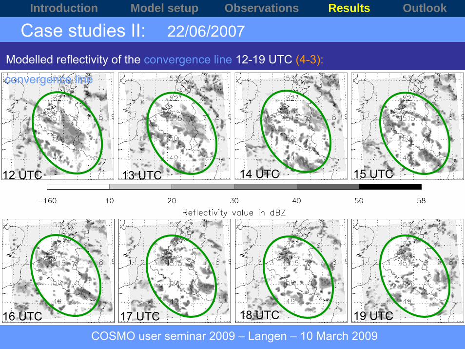
Case studies II: 22/06/2007
Modelled reflectivity of the convergence line 12-19 UTC (4-3):
COSMO user seminar 2009 – Langen – 10 March 2009
convergence line
12 UTC
16 UTC
13 UTC
18 UTC
14 UTC
17 UTC 19 UTC
15 UTC
Introduction Model setup Observations Results Outlook

Case studies II: 22/06/2007
Modelled reflectivity of the convergence line 12-19 UTC (3-21):
COSMO user seminar 2009 – Langen – 10 March 2009
convergence line
12 UTC
16 UTC
13 UTC
18 UTC
14 UTC
17 UTC 19 UTC
15 UTC
Introduction Model setup Observations Results Outlook

Case studies II: 23/06/2007 In the morning and afternoon:convection
COSMO user seminar 2009 – Langen – 10 March 2009
500 hPa geopotential12 UTC
Fronts + surface pressure00 UTC
Introduction Model setup Observations Results Outlook

Case studies II: 23/06/2007
Observed reflectivity of convection 08-15 UTC (radar CAPPI data):
COSMO user seminar 2009 – Langen – 10 March 2009
convection
08 UTC
12 UTC 13 UTC 14 UTC
10 UTC
15 UTC
11 UTC09 UTC
Introduction Model setup Observations Results Outlook

Case studies II: 23/06/2007
Modelled reflectivity of convection 08-15 UTC (4-3):
COSMO user seminar 2009 – Langen – 10 March 2009
convection
12 UTC
08 UTC
13 UTC 14 UTC
10 UTC
15 UTC
11 UTC09 UTC
Introduction Model setup Observations Results Outlook

Case studies II: 23/06/2007
Modelled reflectivity of convection 08-15 UTC (3-21):
COSMO user seminar 2009 – Langen – 10 March 2009
convection
12 UTC
08 UTC
13 UTC 14 UTC
10 UTC
15 UTC
11 UTC09 UTC
Introduction Model setup Observations Results Outlook
COSMO user seminar 2009 – Langen – 10 March 2009
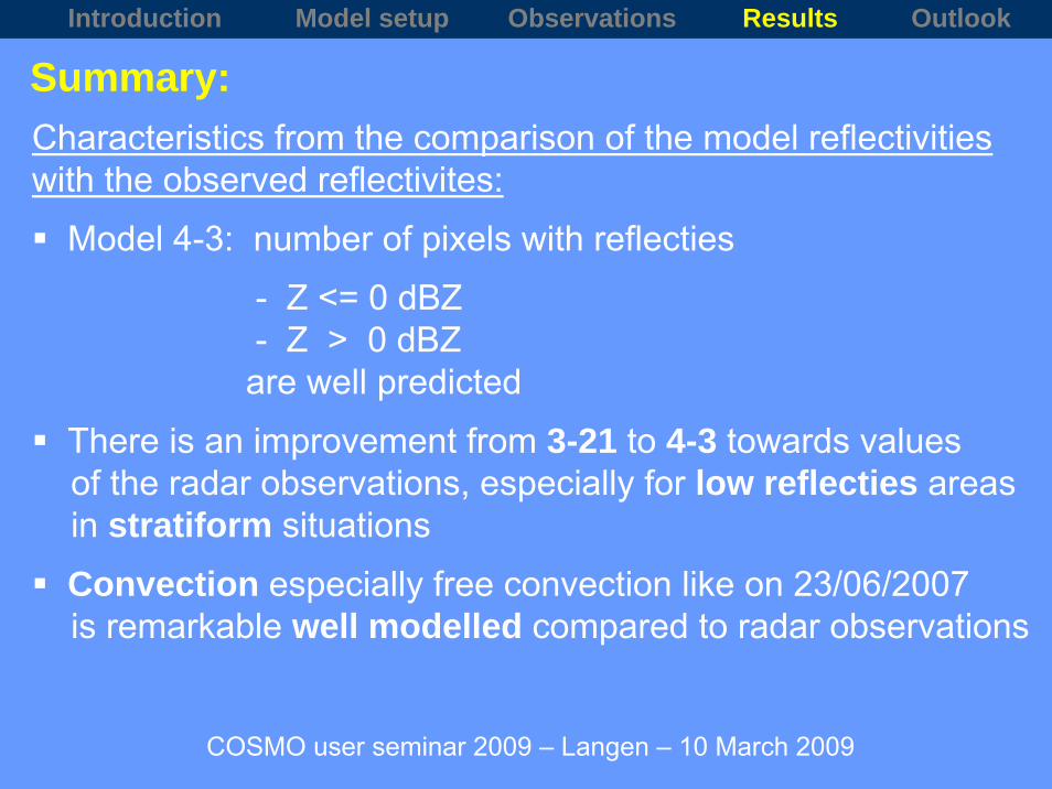
Characteristics from the comparison of the model reflectivities with the observed reflectivites:
Model 4-3: number of pixels with reflecties
- Z <= 0 dBZ - Z > 0 dBZ are well predicted
There is an improvement from 3-21 to 4-3 towards values of the radar observations, especially for low reflecties areas in stratiform situations
Convection especially free convection like on 23/06/2007 is remarkable well modelled compared to radar observations
Summary:Introduction Model setup Observations Results Outlook
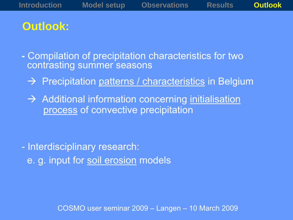
- Compilation of precipitation characteristics for two contrasting summer seasons
Precipitation patterns / characteristics in Belgium
Additional information concerning initialisationprocess of convective precipitation
- Interdisciplinary research:e. g. input for soil erosion models
COSMO user seminar 2009 – Langen – 10 March 2009
Outlook:
Introduction Model setup Observations Results Outlook

Thank you for your attention !!
COSMO user seminar 2009 – Langen – 10 March 2009


Comparison of volume and pseudo CAPPI radar data
Principal characteristics using the 23/11/2006 data set (stratiform precipitation)
COSMO user seminar 2009 – Langen – 10 March 2009
Introduction Model setup Observations Results Outlook

COSMO user seminar 2009 – Langen – 10 March 2009
Radiosonde ascent: Essen, 23/06/2007, 12 UTC:
Introduction Model setup Observations Results Outlook
COSMO user seminar 2009 – Langen – 10 March 2009
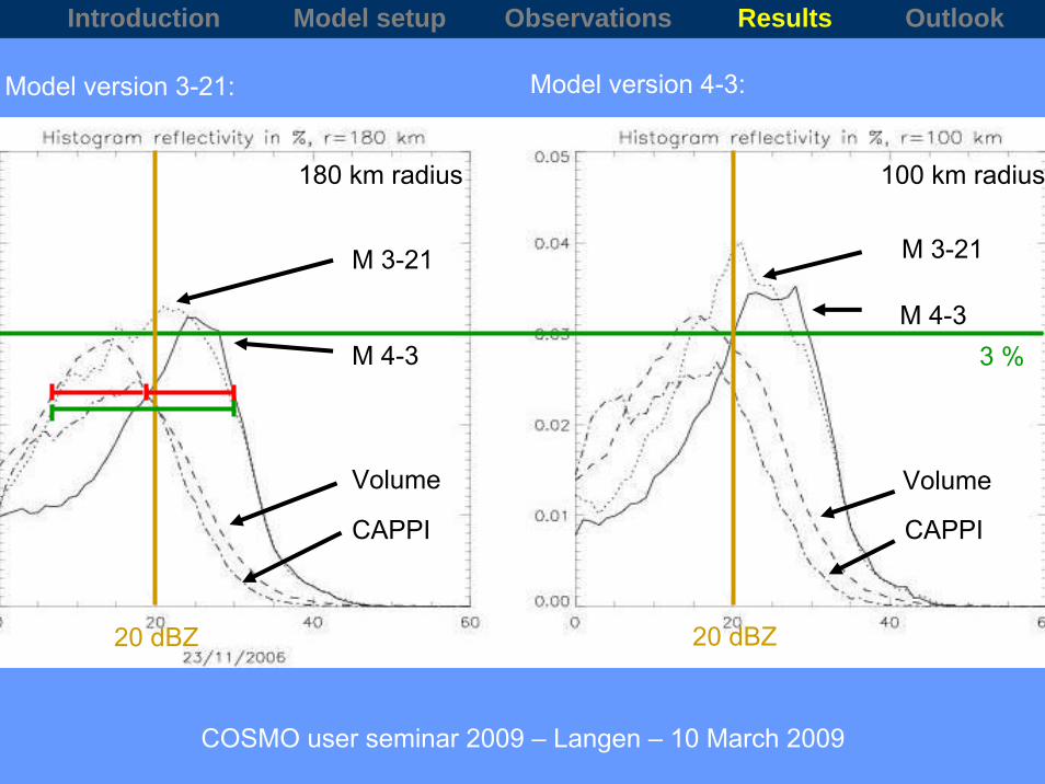
Model version 3-21: Model version 4-3:
180 km radius 100 km radius
20 dBZ 20 dBZ
3 %
M 3-21
M 4-3
Volume
CAPPI
Volume
CAPPI
M 4-3
M 3-21
Introduction Model setup Observations Results Outlook

Data set C-band Doppler Radar:- Volume data and Pseudo CAPPI data
For 2006: Volume data available for WideumontPseudo CAPPI data available for Wideumont
and for ZaventemFor 2007: Volume data in process for Wideumont
Pseudo CAPPI data available for Wideumontand for Zaventem
Volume data: 3D data-set from all radar beam dataPseudo CAPPI data: Pseudo Constant Altitude Plan-
Position Indicator product
Radar data
Introduction Phase I Phase II Summary
COSMO user seminar 2009 – Langen – 10 March 2009
!
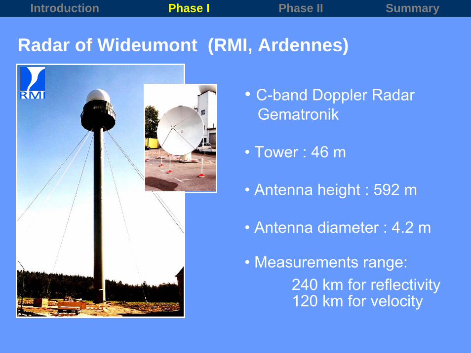
Radar of Wideumont (RMI, Ardennes)
• C-band Doppler Radar Gematronik
• Tower : 46 m
• Antenna height : 592 m
• Antenna diameter : 4.2 m
• Measurements range: 240 km for reflectivity 120 km for velocity
Introduction Phase I Phase II Summary

Radar of Zaventem (BELGOCONTROL, Brussels)
• C-band Doppler Radar Radtec / Sigmet
• Antenna diameter : 4.2 m
• Measurements range:
240 km for reflectivity 120 km for velocity
Introduction Phase I Phase II Summary

Soil erosion in Flanders(Belgium)(Verstraeten et al., 2003)
Orography of Belgium
Introduction Phase I Phase II Summary

~ 250 rain gauge stations in Belgium:
Introduction Phase I Phase II Summary

Introduction Phase I Phase II Summary
COSMO user seminar 2009 – Langen – 10 March 2009
Model version 3-21: Model version 4-3:180 km radius 180 km radius100 km radius 100 km radius
180 km radius 180 km radius100 km radius 100 km radius
20 dBZ 20 dBZ 20 dBZ 20 dBZ
4 %

COSMO user seminar 2009 – Langen – 10 March 2009
Radar volume data: Radar pseudo CAPPI data:180 km radius 180 km radius100 km radius 100 km radius
180 km radius 180 km radius100 km radius 100 km radius
4 %
20 dBZ20 dBZ20 dBZ20 dBZ
Introduction Model setup Observations Results Outlook

COSMO user seminar 2009 – Langen – 10 March 2009
Can these differences be explained by changes in thehydrometeores (e. g. specific snow value) ?
Question:
Next step!!
Introduction Model setup Observations Results Outlook