evaluating the effects of spalling on the capacity of
TRANSCRIPT

Evaluating the Effects of Spalling on the
Capacity of Reinforced Concrete Bridge
Girders
by
Jeffrey Luckai
A thesis
presented to the University of Waterloo
in fulfillment of the
thesis requirement for the degree of
Master of Applied Science
in
Civil Engineering
Waterloo, Ontario, Canada, 2011
©Jeffrey Luckai 2011

ii
Author’s Declaration
I hereby declare that I am the sole author of this thesis. This is a true copy of the thesis,
including any required final revisions, as accepted by my examiners. I understand that my
thesis may be made electronically available to the public.

iii
Abstract
Corrosion of the reinforcing steel is a primary deterioration mechanism for reinforced
concrete bridges. Heavy use of de-icing salts is believed to be a major contributor in Ontario
to severe girder soffit spalling in certain cases. This thesis develops an assessment
methodology to evaluate spalled bridges based on ultimate limit states. Specifically, a
deterministic program is developed for assessment. It is subsequently compared to laboratory
test results and used as a basis for a probabilistic reliability study.
A modified area concept is proposed in this thesis to consider the effects of exposing
reinforcement at various locations along the girder length. A multipoint analysis program,
BEST (Bridge Evaluation Strength Tool), is developed that employs this concept, along with
graphical spalling surveys and structural drawings, to evaluate reinforced concrete bridge
girders. The program is adapted for a full bridge analysis and to consider the other effects of
corrosion, such as bar section loss and bond deterioration.
A case study bridge is evaluated to show that the BEST program offers a viable tool for the
rapid assessment of spalled bridge girders and to facilitate the prioritization of rehabilitation
projects. This evaluation indicates that the spatial distribution of the spalling along a girder,
relative to bar splices and laps, has the most significant influence on structural capacity.
Single girders show strength deficiencies in flexure and shear due to spalling. In general, the
consideration of system effects improves the predicted bridge condition, while considering
section loss and bond deterioration has the opposite effect.
Laboratory work is used to validate the proposed model and identify a number of areas for
future research. The laboratory test results also suggest that the current repair methods are
effective in restoring bond and strength.
In order to further explore potential uses for the BEST program, modifications are made so
that it can be used to perform reliability analyses using Monte-Carlo simulation techniques.

iv
A simplified approach for estimating the reliability index as a function of the deterministic
resistance ratio is proposed based on the reliability analysis results.

v
Acknowledgements
I would like to thank the following parties for their contributions to this work:
Dr. Scott Walbridge and Dr. Maria Anna Polak, co-supervisors of this thesis,
Wade Young, Randy Yu and Andy Turnbull of the Ministry of Transportation of
Ontario for their feedback and support,
Lindsay, Nneka, Nizar, and Lawrence, as well as, Doug Hirst, Robert Sluban and
Richard Morrison for the laboratory assistance,
Sika Canada and HOGG Fuel & Supply Ltd. for material donations, and
my family, friends and colleagues at UW for their support.

vi
Dedication
To My Parents
vii
Table of Contents
Author‘s Declaration ................................................................................................................. ii
Abstract .................................................................................................................................... iii
Acknowledgements ................................................................................................................... v
Dedication ................................................................................................................................ vi
Table of Contents .................................................................................................................... vii
List of Figures .......................................................................................................................... xi
List of Tables .......................................................................................................................... xv
Chapter 1 Introduction .............................................................................................................. 1
1.1 General ............................................................................................................................ 1
1.2 Research Objectives ........................................................................................................ 3
1.3 Scope ............................................................................................................................... 4
1.4 Thesis Organization......................................................................................................... 5
Chapter 2 Background and Literature Review.......................................................................... 6
2.1 Deterioration of Concrete Bridges .................................................................................. 6
2.1.1 Corrosion .................................................................................................................. 6
2.1.2 Corrosion Accelerators/Instigators ........................................................................... 8
2.1.3 Damage Manifestation ............................................................................................ 10
2.1.4 Phases of Corrosion in Concrete Structures ........................................................... 12
2.2 Impacts of Deterioration on Structural Performance .................................................... 16
2.2.1 Reinforcing Steel Deterioration .............................................................................. 16
2.2.2 Concrete/Steel Bond Loss ...................................................................................... 21
2.2.3 Composite Action ................................................................................................... 27
2.3 Summary ....................................................................................................................... 31
Chapter 3 Structural Strength Assessment .............................................................................. 33
3.1 Introduction ................................................................................................................... 33
3.2 Case Study Structure ..................................................................................................... 33
3.2.1 Background ............................................................................................................. 34
3.2.2 Deterioration ........................................................................................................... 35
viii
3.2.3 Available Resources ............................................................................................... 36
3.2.4 Structural Analysis ................................................................................................. 38
3.3 Modified Strength Concept ........................................................................................... 40
3.3.1 CSA Development Length ...................................................................................... 41
3.3.2 Modified Area Concept .......................................................................................... 42
3.4 Modified Moment Resistance ....................................................................................... 43
3.4.1 CSA Moment Capacity ........................................................................................... 44
3.4.2 Modified Moment Capacity .................................................................................... 45
3.5 Modified Shear Resistance ............................................................................................ 47
3.5.1 CSA Shear Capacity ............................................................................................... 48
3.5.2 Modified Shear Capacity based on CSA Simplified Method ................................. 49
3.5.3 Modified Shear Capacity based on CSA General Method ..................................... 51
3.6 Reliability Analysis ....................................................................................................... 52
3.6.1 CSA Target Reliability Index ................................................................................. 52
3.6.2 CSA Reliability Evaluation .................................................................................... 55
3.6.3 Reliability of Deteriorated Bridge .......................................................................... 57
3.6.4 Full Bridge Reliability ............................................................................................ 58
Chapter 4 Deterministic Analysis and Results........................................................................ 61
4.1 Introduction ................................................................................................................... 61
4.2 Single Girder Matlab Program ...................................................................................... 61
4.2.1 Modified Area......................................................................................................... 61
4.2.2 Moment Resistance................................................................................................. 64
4.2.3 Simplified Method Shear Resistance ...................................................................... 66
4.2.4 Shear Resistance General Method .......................................................................... 69
4.2.5 Reliability Index ..................................................................................................... 71
4.3 Full Bridge Analysis Program ....................................................................................... 72
4.4 Sensitivity Analysis ....................................................................................................... 77
4.4.1 Variation of f‘c ....................................................................................................... 77
4.4.2 Future Deterioration Estimate ................................................................................ 79
4.5 Corrosion Section Loss Model ...................................................................................... 79
ix
4.5.1 Corrosion Model Input ........................................................................................... 80
4.5.2 Corrosion Model Output ......................................................................................... 81
4.6 Bond Deterioration Model ............................................................................................ 82
4.6.1 Program Applications ............................................................................................. 85
4.6.2 Program Limitations ............................................................................................... 87
Chapter 5 Experimental Program and Results ........................................................................ 88
5.1 Introduction ................................................................................................................... 88
5.2 Test Program ................................................................................................................. 88
5.2.1 Test Specimens ....................................................................................................... 90
5.2.2 Material Properties ................................................................................................. 90
5.2.3 Deterioration ........................................................................................................... 91
5.2.4 Instrumentation ....................................................................................................... 92
5.2.5 Rehabilitation.......................................................................................................... 92
5.3 Test Results and Discussion .......................................................................................... 94
5.3.1 Reference Beam ...................................................................................................... 94
5.3.2 Spalling Series ........................................................................................................ 95
5.3.3 Rehabilitation Series ............................................................................................... 99
5.4 Summary ..................................................................................................................... 101
Chapter 6 Reliability Analysis .............................................................................................. 103
6.1 Introduction ................................................................................................................. 103
6.2 Probabilistic Analysis Methods ................................................................................... 103
6.3 Statistical Modelling of Input Parameters ................................................................... 106
6.3.1 Statistical Resistance Modelling ........................................................................... 107
6.3.2 Statistical Solicitation (i.e. Load) Modelling........................................................ 111
6.4 Reliability Index Results ............................................................................................. 112
6.4.1 Single Girder: Flexure .......................................................................................... 112
6.4.2 Single Girder: Shear Simplified Method .............................................................. 114
6.4.3 Single Girder: Shear General Method .................................................................. 117
6.4.4 Single Girder: Total Reliability ............................................................................ 118
Chapter 7 Conclusions and Recommendations ..................................................................... 121

x
7.1 Conclusions ................................................................................................................. 121
7.1.1 Deterministic Analysis ......................................................................................... 121
7.1.2 Laboratory Work .................................................................................................. 122
7.1.3 Reliability Analysis .............................................................................................. 123
7.2 Recommendations for Future Work ............................................................................ 123
7.2.1 Further Development of BEST Computer Program ............................................. 123
7.2.2 Extension of Laboratory Studies .......................................................................... 124
7.2.3 Further Investigation of Rehabilitation Methods.................................................. 125
7.2.4 Improvements in Corrosion Measurement ........................................................... 126
7.2.5 Effect of Corrosion on Other Components ........................................................... 127
Bibliography ......................................................................................................................... 129
Appendix A ........................................................................................................................... 136
Appendix B ........................................................................................................................... 155
Appendix C ........................................................................................................................... 172
Appendix D ........................................................................................................................... 179

xi
List of Figures
Figure 2-1: Schematic of micro-cell corrosion (Hansson et al. 2006). ..................................... 7
Figure 2-2: Schematic of macro-cell corrosion (Hansson et al. 2006). .................................... 8
Figure 2-3: Rust expansion and resulting: (a) Inclined fracture plane; (b) Parallel fracture
plane (Li et al. 2007). .............................................................................................................. 10
Figure 2-4: Mapping of corrosion cracking on specimens by Rodriguez et al. (1997). ........ 11
Figure 2-5: Bridge girder spalling and delamination (MTO). ................................................ 11
Figure 2-6: Residual section loss for the (a) Uniform and (b) Localized corrosion
(CONTECVET 2001). ............................................................................................................ 12
Figure 2-7: Phases of corrosion in concrete structures (CONTECVET 2001). ...................... 12
Figure 2-8: Effects of reinforcement corrosion on residual structural capacity (Cairns et al.
2005a). .................................................................................................................................... 16
Figure 2-9: Empirical models for residual yield strength of corroded bars. ........................... 18
Figure 2-10: Empirical models for residual ultimate strength of corroded bars. .................... 20
Figure 2-11: Empirical models for residual ultimate elongation of corroded bars. ................ 20
Figure 2-12: Bond strength with corrosion. (a) Pullout and (b) Flexure test results (Bhargava
et al. 2007). ............................................................................................................................. 22
Figure 2-13: (a) Forces acting on rib and (b) Resolution of radial bursting forces (Cairns and
Abdullah 1996 as cited by Bhargava et al. 2007). .................................................................. 24
Figure 2-14: Bond failure modes of ribbed reinforcing bars by (Cairns and Abdullah 1996).
................................................................................................................................................. 24
Figure 2-15: Empirical models for steel-concrete bond deterioration. ................................... 26
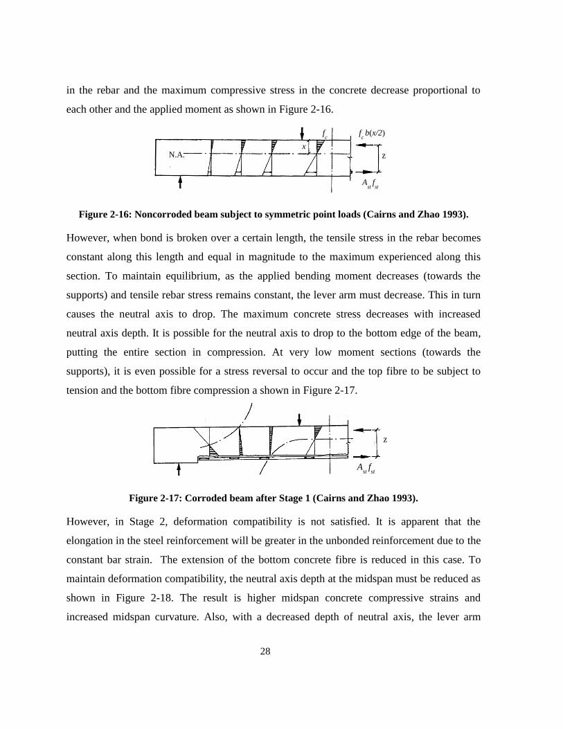
Figure 2-16: Noncorroded beam subject to symmetric point loads (Cairns and Zhao 1993). 28
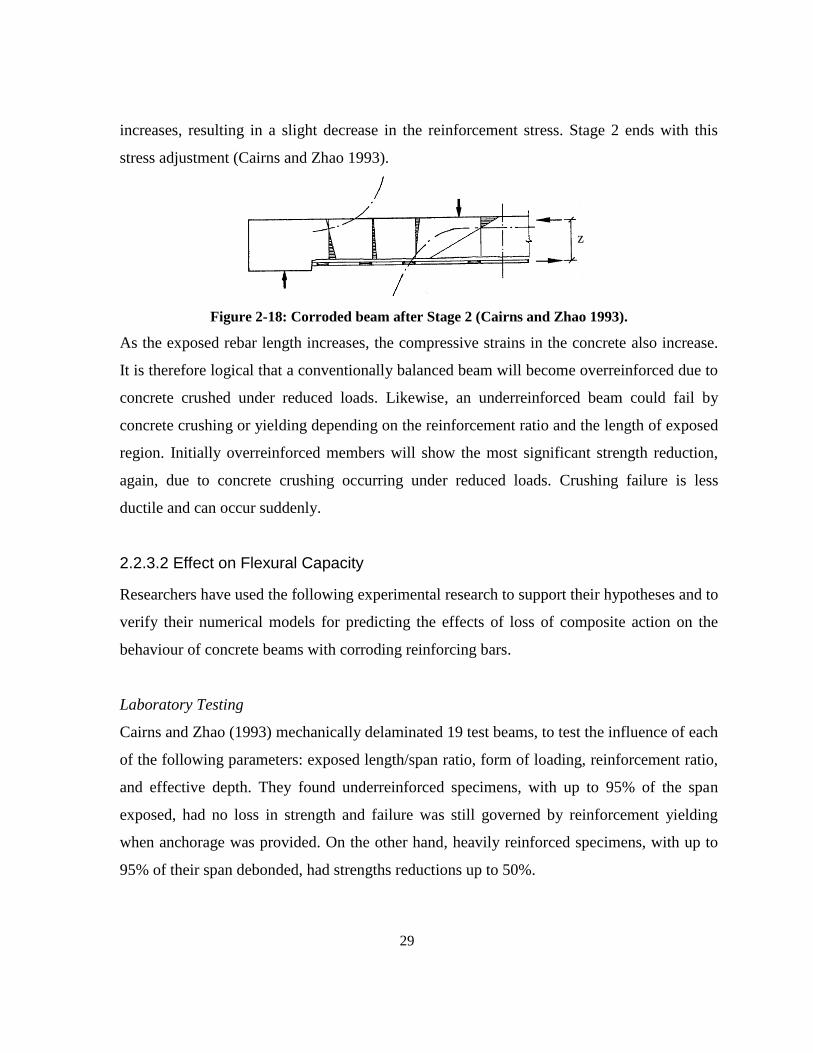
Figure 2-17: Corroded beam after Stage 1 (Cairns and Zhao 1993). ...................................... 28
Figure 2-18: Corroded beam after Stage 2 (Cairns and Zhao 1993). ...................................... 29
Figure 3-1: Case study structure (a) Cross section, and (b) Elevation. ................................... 34
Figure 3-2: Girder spalling and delamination. ........................................................................ 36
Figure 3-3: Spalling survey sample (August 2009). ............................................................... 37
Figure 3-4: Scaling operation (MTO). .................................................................................... 37
Figure 3-5: Spalling/reinforcement superposition. ................................................................. 38

xii
Figure 3-6: SAP2000 model. .................................................................................................. 39
Figure 3-7: Live load (unfactored) moment envelope. ........................................................... 39
Figure 3-8: Live load (unfactored) shear envelope. ................................................................ 40
Figure 3-9: Modified area concept. ......................................................................................... 42
Figure 3-10: Rectangular stress block theory for flexural design of an RC member. ............ 44
Figure 3-11: Moment resistance of unspalled and spalled bars. ............................................. 46
Figure 3-12: Basic shear resisting mechanism assumed by Bentz (2006). ............................. 47
Figure 3-13: Relationship between risk and reliability (CAN/CSA S6-06). .......................... 53
Figure 3-14: Load factors for various target reliability indices. ............................................. 56
Figure 3-15: Slab strength evaluation. .................................................................................... 59
Figure 3-16: Girder grouping for full structure analysis. ........................................................ 60
Figure 4-1: Algorithm for the computation of the modified area. .......................................... 62
Figure 4-2: Reinforcement plan-spalling survey superposition for program input. ............... 63
Figure 4-3: Algorithm for the computation of flexural capacity using the modified area
concept. ................................................................................................................................... 64
Figure 4-4: Flexural evaluation of Girder 2. ........................................................................... 66
Figure 4-5: Algorithm for the computation of the shear capacity using the Simplified Shear
Method. ................................................................................................................................... 67
Figure 4-6: Shear evaluation of Girder 2: Simplified Method. ............................................... 68
Figure 4-7: Algorithm for the computation of the shear capacity using the General Shear
Method. ................................................................................................................................... 69
Figure 4-8: Shear evaluation of Girder 2: General Method. ................................................... 70
Figure 4-9: Effect of the loss of anchorage on Girder 2 of the case study structure. ............. 71
Figure 4-10: Approximate reliability index of Girder 2. ........................................................ 72
Figure 4-11: Algorithm and file organization for multi-girder analysis. ................................ 73
Figure 4-12: Spalled moment resistance for each girder in the bridge. .................................. 74
Figure 4-13: Minimum spalled girder resistance for (a) Flexure, (b) Simplified Shear and (c)
General Shear Methods. .......................................................................................................... 75
Figure 4-14: Full bridge case study structure analysis using girder grouping presented as
resistance ratio. ....................................................................................................................... 76
xiii
Figure 4-15: Full bridge approximate reliability. ................................................................... 77
Figure 4-16: Spalling scale-up analysis. ................................................................................. 79
Figure 4-17: Selected empirical model for residual yield strength of corroded bars.............. 80
Figure 4-18: Full bridge resistance ratio with section loss model. ......................................... 81
Figure 4-19: Full bridge reliability with section loss model. .................................................. 82
Figure 4-20: Selected empirical relationship for steel deterioration. ...................................... 83
Figure 4-21: Full bridge resistance ratio with section loss and bond deterioration. ............... 84
Figure 4-22: Full bridge reliability with section loss and bond deterioration. ........................ 85
Figure 4-23: Moment and shear envelopes for a 3-span continuous girder. ........................... 86
Figure 5-1: Typical test specimen (a) Cross section and (b) Elevation. ................................. 90
Figure 5-2: Cast-in foam blocks for spalling simulation. ....................................................... 91
Figure 5-3: Surface roughened by needle peener and strain gauge installation. .................... 91
Figure 5-4: SikaTop 123 application. ..................................................................................... 92
Figure 5-5: Sikacrete-08 SCC application. ............................................................................. 93
Figure 5-6: Beam 6 intact section cracking. ........................................................................... 98
Figure 5-7: Spalling Series load-deflection curves for (a) Spalling configurations and (b)
Arch action. ............................................................................................................................. 99
Figure 5-8: Rehabilitation Series load-deflection curves for (a) Sikacrete, FRP and (b) SCC
repairs. ................................................................................................................................... 101
Figure 6-1: Probability density for G. ................................................................................... 104
Figure 6-2: Probabilistic variables for bridge resistance. ..................................................... 106
Figure 6-3: Probabilistic variables for bridge solicitation. ................................................... 106
Figure 6-4: Flexural reliability index. ................................................................................... 112
Figure 6-5: Reliability Index determined by MCS analysis at critical section. .................... 113
Figure 6-6: MCS vs. approximate reliability analysis for flexure. ....................................... 114
Figure 6-7: Probability of failure for shear (Simplified Method) using MCS. ..................... 115
Figure 6-8: Reliability Index for shear (Simplified Method) using MCS. ........................... 115
Figure 6-9: Full vs. approximate reliability analysis for Simplified Shear Method. ............ 116
Figure 6-10: Shear (General Method) reliability index. ....................................................... 117
Figure 6-11: Resistance ratio and reliability index for flexure and shear. ............................ 119

xiv
Figure 6-12: Resistance ratio and reliability index for both analyses. .................................. 119
Figure 7-1: Specimen design for intact length (X) analysis. ................................................. 125
Figure 7-2: Test specimen for partial spalling evaluation. ................................................... 125
Figure 7-3: Proposed detail for splice repair evaluation. ...................................................... 126
Figure 7-4: Concept for reinforcement corrosion pit gauge. ................................................ 127
Figure 7-5: Corrosion cracking, surface staining and section loss. ...................................... 127
Figure 7-6: Severe slab spalling (MTO). .............................................................................. 128

xv
List of Tables
Table 2.1: Input for bond degradation model comparison. ..................................................... 26
Table 3.1: System behaviour (CAN/CSA S6-06). .................................................................. 53
Table 3.2: Element behaviour (CAN/CSA S6-06). ................................................................ 53
Table 3.3: Inspection level (CAN/CSA S6-06). ..................................................................... 54
Table 3.4: Target reliability index, β, for normal traffic and for PA, PB, and PS traffic
(CAN/CSA S6-06). ................................................................................................................. 54
Table 3.5: Reliability index factors for the case study structure. ............................................ 55
Table 3.6: Dead load components for evaluation (CAN/CSA S6-06). ................................... 55
Table 3.7: Maximum dead load factors, D (CAN/CSA S6-06). ........................................... 55
Table 3.8: Live load factors, L, for normal traffic (evaluation levels 1, 2, and 3) for all types
of analysis (CAN/CSA S6-06). ............................................................................................... 56
Table 4.1: Variation of fc’ results. .......................................................................................... 78
Table 5.1: Test matrix. ............................................................................................................ 89
Table 5.2: Strength approximations of Beam 1. ..................................................................... 94
Table 5.3: Strength approximation for spalling series beams. ................................................ 95
Table 5.4: Test specimen crack patterns. ................................................................................ 97
Table 5.5: Rehabilitation series test results........................................................................... 100
Table 6.1: Relationship between probability of failure and reliability index (CAN/CSA S6).
............................................................................................................................................... 105
Table 6.2: Acceptable degree of risk in society (MacGregor 1976). .................................... 105
Table 6.3: Bias Factors for probabilistic analysis. ................................................................ 107
Table 6.4: Critical section in flexure reliability: Analysis summary. ................................... 113
Table 6.5: Critical section in shear (Simplified Method) reliability: Analysis summary. .... 116
Table 6.6: Critical section in shear (General Method) reliability analysis summary. .......... 117

1
Chapter 1
Introduction
1.1 General
In the Province of Ontario, as in the rest of North America, the assessment and maintenance
of existing highway bridges is currently an area of significant concern (Council of the
Federation 2005). It is widely agreed that the condition of these structures is deteriorating
over time. The following paragraphs discuss the current state of Ontario‘s highway bridge
infrastructure.
Ontario’s Highway Bridges
Ontario has approximately 14800 road bridges in total. Approximately 12000 of these are
located within municipalities, while 2800 are owned and maintained by the province (Aud.
2009). Of the provincially managed bridges, more than 70% were built between 1950 and
1980 with an average age of approximately 40 years. The majority of municipal bridges in
Ontario are slightly older with an average age of 43 years (Aud. 2009).
Many of the bridges requiring repair and rehabilitation in Ontario are located along major
highways. In the Greater Toronto Area there are over 660 bridges on 400 series highways,
some of which span over up to 16 lanes of traffic (Aud. 2009).
Work Backlog
A number of sources have indicated that there currently is a backlog in bridge maintenance
and repair in Ontario. According to the Ontario Ministry of Transportation (MTO) current
assessment methodology, more than 180 or 7% of provincial bridges were in poor condition,
which is defined by MTO as requiring repair or rehabilitation work within one year of the
inspection, and 17% (or 471 bridges) were in fair condition (Aud. 2009). A 2009 review by
the Ontario Auditor General (Aud. 2009) found that around 60% of the bridges rated in fair
or poor condition by MTO were not on the Ministry‘s five-year capital work plan. The same

2
report found that approximately 85% of the municipalities responding to the survey
confirmed that they had a backlog of rehabilitation work. Of those, 45% had 1-5 year
backlogs, 25% had 6-10 year backlogs, and 10% had work backlogs of over 10 years.
Funding
Economic conditions have greatly influenced infrastructure spending in Canada and Ontario.
Infrastructure spending in Ontario has annually increased over the past three years. In 2010-
2011 the Renew Canada program (Renew 2009) boasted $4.53 billion in funding for
transportation investments. Of this amount, 44% was dedicated for provincial highways. An
increase in funding for transportation and transit to $5.40 billion is expected for 2011-2012
(39% will be dedicated to provincial highways).
In 2009, MTO estimated that the cost of repair and rehabilitation of its structures in either
fair or poor condition over the next five year period (from 2009) to be approximately $2.2
billion, yet the Ministry budget for bridge work over the same period was only $1.4 billion.
Industry Challenges
Aging infrastructure is the primary challenge currently facing Ontario bridge managers,
including MTO. It is expected that there will be a spike in the need for major repair and
rehabilitation work over the next 6-10 years (based the average structure age).
Due to the quantity of work in Ontario, a shortage of available specialized contractors has
developed. Project costs have also escalated due to a lack of competition created in part by
the consolidation of the consulting industry, and the result of a market that is flooded by local
government spending (Aud. 2009).
In urban areas, a steady increase in congestion has increased the need for highway expansion.
When roadway expansion is anticipated, as it currently is in the foreseeable future, bridge
3
replacement is delayed and the need for structural assessment and repair increases. To
complicate matters, structural repair and replacement by conventional means often requires
expensive highway closures, and work of this nature is difficult and time consuming
(personal correspondence, R. Yu 2010).
As a result, there is currently an emphasis on the need to develop better assessment and
repair methods for bridge structures. At this time, many reports indicate that bridge
inspectors are unable to distinguish between many visible deterioration effects and those that
actually have a significant impact of the safety of the public (Aud. 2009). In particular,
surface spalling of reinforced concrete (RC) bridge girders, at this time, due to the
uncertainty of its impact on structural capacity, often falls within the realm of ―routine
maintenance‖ work, when in fact it should first be evaluated based on the estimated residual
strength and safety of the structure.
1.2 Research Objectives
Based on the discussion in the previous section, the objectives of the research project
summarized in the current thesis are as follows:
1) execution of a field survey of RC bridges with varying levels of deterioration, to
assess the significance of the problem and determine what information bridge
inspectors have at their disposal when carrying out a bridge assessment,
2) development of deterministic and probabilistic prediction models for evaluating the
safety of RC flexural members with exposed reinforcement, and
3) initial study and evaluation of a number of alternative simple, rapid, and cost effective
rehabilitation methods for RC bridges with spalled concrete.
4
1.3 Scope
The scope of the current thesis is limited to the assessment and rehabilitation of multi-girder
RC highway bridges without prestressing. The studied deterioration is limited to soffit
spalling of primary girder elements. Shear and moment resistance models for beams are used
in the developed assessment program, meaning that the beneficial effects of arch action are
not considered. The presented assessment program research focuses on the development of a
simple, rapid assessment tool, employing code-like models and modified design formulas
that are already familiar to structural engineers. The developed assessment program is
verified by comparison with results of a small-scale laboratory study. Extension of the
developed assessment program for applications involving prestressed girders or two-way
structural systems (e.g. deck slabs) is beyond the scope of the current thesis.

5
1.4 Thesis Organization
This thesis is organized into seven chapters, as follows:
In Chapter 2, relevant background information and a state-of-the art literature review are
presented, to introduce important concepts related to the research.
Next, in Chapter 3, a field survey is used to develop the concepts employed in the current
thesis for the strength assessment of deteriorated RC bridge structures.
In Chapter 4, the implementation of these concepts in a computer assessment program is
discussed and the program application is demonstrated using a case study structure.
In Chapter 5 a pilot laboratory study is presented, wherein several spalling configurations
and rehabilitation approaches are tested.
In Chapter 6, the program is modified to facilitate the full reliability (i.e. probabilistic)
analysis of single girders in spalled RC bridge structures.
Finally, conclusions and recommendations are presented in Chapter 7.
6
Chapter 2
Background and Literature Review
2.1 Deterioration of Concrete Bridges
2.1.1 Corrosion
In general, the corrosion of steel reinforcement is primarily responsible for surface spalling
and is highly detrimental to our infrastructure. To understand the effects of corrosion on the
residual capacity of a reinforced concrete member, it is prudent to first understand the cause.
This section presents a brief background of steel corrosion and describes the main causes of
concrete deterioration.
2.1.1.1 Corrosion Reaction
Concrete is naturally a non-corrosive environment for steel due to its high alkalinity (ph >
13). Initially, the concrete creates a passive layer around the embedded reinforcement that is
capable of effectively protecting the steel reinforcing bars. However, from the time of
casting, corrosion accelerators, such as chlorides or carbon dioxide, start to penetrate the
concrete cover and act to lower the ph of the concrete surrounding the reinforcement, thus
triggering corrosion.
The corrosion of steel reinforcement coincides with the formation of a rust layer on the steel
surface. The formation of rust can be characterized by the following reactions (Hansson et al.
2007):
2
2Fe 2OH Fe OH (3.1)
2 22 34Fe OH O 2H O 4F+ e OH (3.2)
7
2 3 2 232Fe OH Fe O H O 2H O (3.3)
In the corrosion reactions, iron ions react with hydroxide ions and dissolved oxygen to form
iron oxides and hydroxides. Hydration of the ferric hydroxide compounds forms ferric oxide
or red rust. If the passive layer is uniform, continuous and dense, then corrosion may be
stifled or negated under natural conditions. In a concrete member, according to Hansson et al.
(2006), corrosion occurs either on a micro or macro cell level.
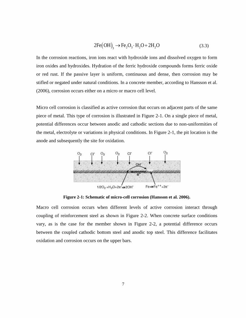
Micro cell corrosion is classified as active corrosion that occurs on adjacent parts of the same
piece of metal. This type of corrosion is illustrated in Figure 2-1. On a single piece of metal,
potential differences occur between anodic and cathodic sections due to non-uniformities of
the metal, electrolyte or variations in physical conditions. In Figure 2-1, the pit location is the
anode and subsequently the site for oxidation.
Figure 2-1: Schematic of micro-cell corrosion (Hansson et al. 2006).
Macro cell corrosion occurs when different levels of active corrosion interact through
coupling of reinforcement steel as shown in Figure 2-2. When concrete surface conditions
vary, as is the case for the member shown in Figure 2-2, a potential difference occurs
between the coupled cathodic bottom steel and anodic top steel. This difference facilitates
oxidation and corrosion occurs on the upper bars.
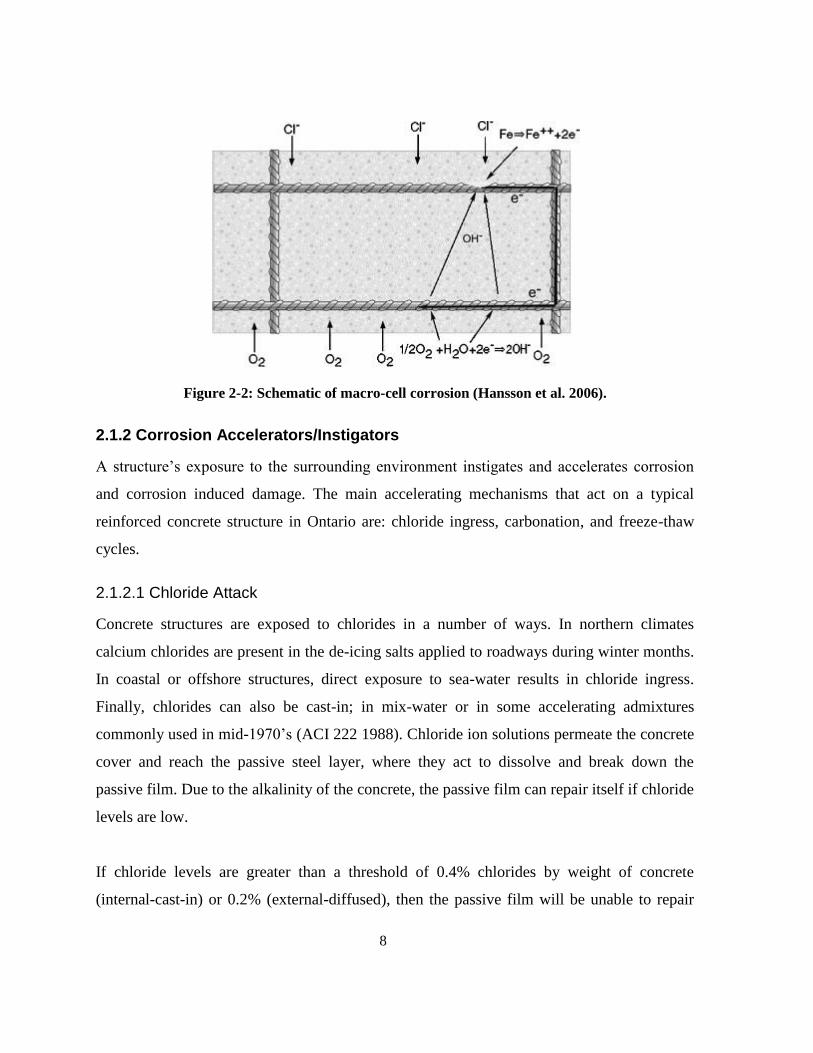
8
Figure 2-2: Schematic of macro-cell corrosion (Hansson et al. 2006).
2.1.2 Corrosion Accelerators/Instigators
A structure‘s exposure to the surrounding environment instigates and accelerates corrosion
and corrosion induced damage. The main accelerating mechanisms that act on a typical
reinforced concrete structure in Ontario are: chloride ingress, carbonation, and freeze-thaw
cycles.
2.1.2.1 Chloride Attack
Concrete structures are exposed to chlorides in a number of ways. In northern climates
calcium chlorides are present in the de-icing salts applied to roadways during winter months.
In coastal or offshore structures, direct exposure to sea-water results in chloride ingress.
Finally, chlorides can also be cast-in; in mix-water or in some accelerating admixtures
commonly used in mid-1970‘s (ACI 222 1988). Chloride ion solutions permeate the concrete
cover and reach the passive steel layer, where they act to dissolve and break down the
passive film. Due to the alkalinity of the concrete, the passive film can repair itself if chloride
levels are low.
If chloride levels are greater than a threshold of 0.4% chlorides by weight of concrete
(internal-cast-in) or 0.2% (external-diffused), then the passive film will be unable to repair
9
itself (Hope and Ip 1987). Once they reach the steel, chlorides are not consumed in the
reaction; rather they act as a catalyst for the cathode reaction (oxygen consumption). Since
the chloride ion concentration that reaches the steel and the subsequent breakdown of the
passive layer is not uniform, chloride induced corrosion is highly localized and leads to
pitting.
2.1.2.2 Carbonation
Carbon dioxide, found in air, can dissolve in concrete pore water to form carbonic acid. This
carbonic acid can react with cement hydration products, i.e. calcium hydroxide, and reduce
the alkalinity of the concrete according to the following reaction (Hansson et al. 2007):
2 2 3 22CO H O Ca OH CaCO 2H O (3.4)
At the reinforcement, depassivation occurs due to the imposed acidity, and corrosion can
begin with the presence of moisture and oxygen. It should be noted that the process is
relatively slow compared to chloride induced corrosion and occurs uniformly over the bar
length. Therefore, corrosion by carbonation is often referred to as homogeneous corrosion.
2.1.2.3 Freeze-Thaw
Persistent cycles of freeze-thaw can be devastating to concrete structures in northern
climates. During mild cycles, a water chloride solution enters the concrete pores, freezing
when temperatures drop below zero. The change of state attacks both the concrete paste and
aggregate. The scientific explanation of the cracking and spalling caused by freeze-thaw
varies significantly.
Powers (1945) hypothesized that freeze-thaw damage was caused by hydraulic pressure
(internal stresses) created by the volumetric increase of water freezing to ice within concrete
pores and considered the role of chlorides with the osmotic potential concept (Powers 1975).
Litvan (1972) suggested that water absorbed within small pores cannot freeze in-situ due to
surface/water interactions (Van der Waals forces) and thus a vapour pressure deference
exists.

10
Mindless and Young (1981) and Pigeon and Pleau (1995) suggest that the solution saturating
the pores, within the concrete, immediately below the surface, has a high chloride
concentration. On the surface the water is pure, resulting in a difference in freezing points
and vapour pressures, creating surface scaling. Other researchers believe the opposite occurs
and the solution is highly concentrated outside the pores. Throughout the chloride application
and freeze-thaw cycles experienced over a structure‘s lifetime it is likely that several
deterioration mechanisms exist.
2.1.3 Damage Manifestation
The effects of corrosion of the reinforcing steel (rebar) on the deterioration of reinforced
concrete structures are: steel section loss, concrete cracking and spalling or delamination
(Cairns et al. 2008).
Concrete Cracking
When reinforcing steel corrodes, the resulting corrosion products can have a volume of up to
six times that of the original material (Herholdt et al. 1985). This volume increase causes
radial tensile stresses on the surrounding concrete as shown in Figure 2-3. When these
stresses exceed the concrete tensile strength, cracking occurs. The most common form of
cracking consists of longitudinal cracks at the height of the reinforcement layer as shown in
Figure 2-4.
a) (b)
Figure 2-3: Rust expansion and resulting: (a) Inclined fracture plane; (b) Parallel fracture
plane (Li et al. 2007).
rust expansion
force rust expansion
force
S
C
crack
crack
C
ft f
t
ft f
t
rust expansion
force
11
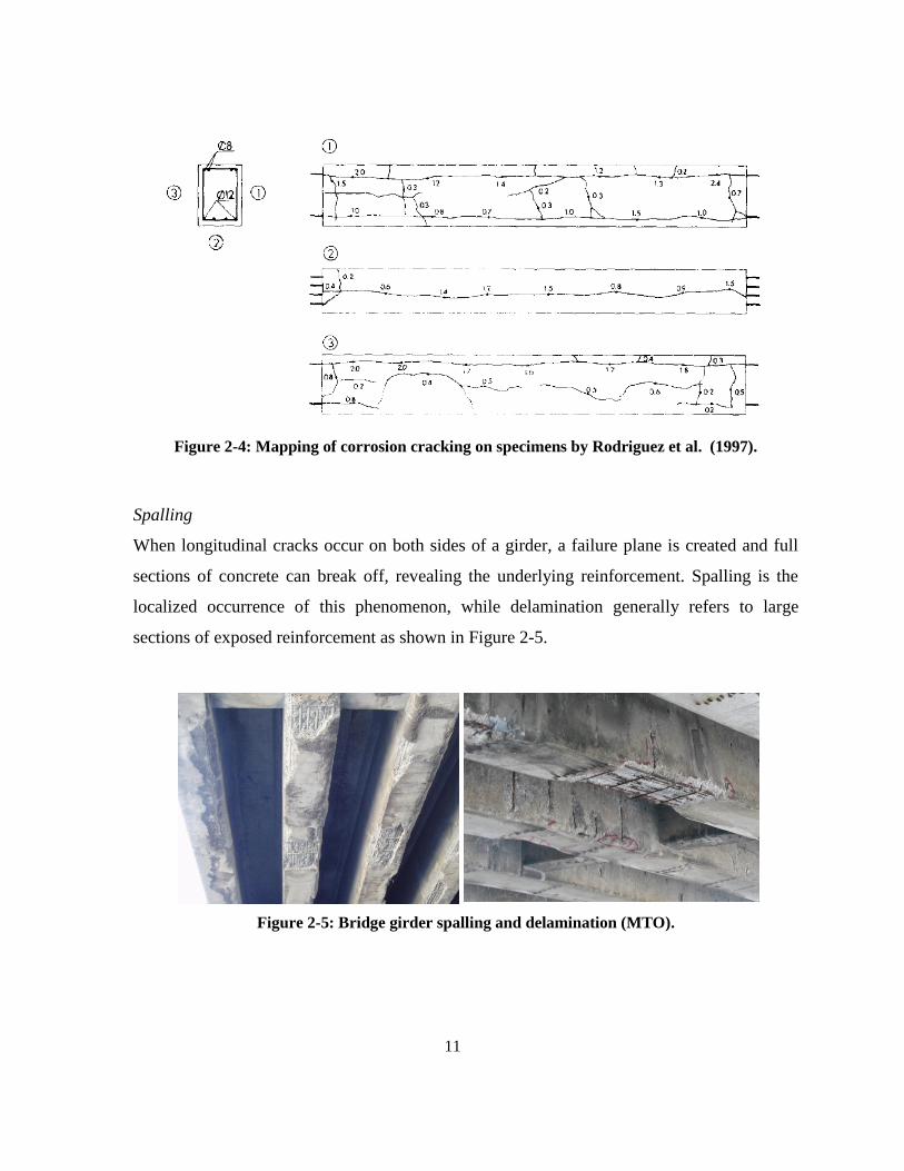
Figure 2-4: Mapping of corrosion cracking on specimens by Rodriguez et al. (1997).
Spalling
When longitudinal cracks occur on both sides of a girder, a failure plane is created and full
sections of concrete can break off, revealing the underlying reinforcement. Spalling is the
localized occurrence of this phenomenon, while delamination generally refers to large
sections of exposed reinforcement as shown in Figure 2-5.
Figure 2-5: Bridge girder spalling and delamination (MTO).

12
Steel Section Loss
In the corrosion reaction, steel is consumed. Chloride induced corrosion tends to result in
pitting or localized steel consumption, while carbonation tends to produce a generalized
deterioration as shown in Figure 2-6.
(a) (b)
Figure 2-6: Residual section loss for the (a) Uniform and (b) Localized corrosion
(CONTECVET 2001).
2.1.4 Phases of Corrosion in Concrete Structures
The corrosion process is divided into a two phase process by Tuutti (1982): initiation and
propagation. These two phases are depicted graphically in Figure 2-7.
Figure 2-7: Phases of corrosion in concrete structures (CONTECVET 2001).
Acceptable Degree of Damage
Time (t)
Cl- Diffusion
CO2 Diffusion
Initiation Propagation
Lifetime or Time before Repair
Cracking
Spalling
Deg
ree
of
Co
rro
sio
n

13
2.1.4.1 Initiation
The initiation phase represents the time for either chlorides or carbonation (or both) to
permeate the concrete cover, reach the steel, and overcome the threshold levels. It extends
from the time of construction to the time T1, which is generally approximated by modelling
the diffusion of contaminants through the concrete cover.
Chloride Diffusion
For chloride diffusion in concrete, Fick‘s second law of diffusion is commonly adopted
(Andrade 1993):
(1 erf )2
x s
c
xC C
D t
(3.5)
where:
t = time in seconds
Dc = diffusion coefficient (0.1− 3.0∙10-12
m2/s)
x = depth of Cl- level
CS = Cl- content @ surface
Cx = Cl- content @ depth x
erf = Gauss error function
Theoretically, the initiation time depends on:
chloride or carbon dioxide concentration in contact with concrete,
permeability, w/c ratio, and quality of the concrete,
amount of moisture present,
concrete alkalinity (ph, passive layer),
concrete cover, and
quantity and severity of flexural cracks.

14
Carbonation
A simple model for carbonation diffusion is the square root method (CONTECVET 2001),
where:
=x V t (3.6)
where,
t = time in seconds
x = penetration depth of carbonation
V = velocity of advance = '
c
172 0.126 for RH 50%
f
Linear reductions may be used for RH greater or less than 50%. Four other models are
suggested in (CONTECVET 2001).
2.1.4.2 Propagation
The propagation or active corrosion stage, Tcorr, extends from the time of first formation of
corrosion products, depassivation, or the end of initiation to a difficult to define state
generally referred to as the end of service life. The following are some examples of the
different definitions for the end of propagation:
the time when corrosion generates sufficient stress to crack or spall the concrete
cover, or the local attack on the reinforcement becomes sufficiently severe as to
impair its load carrying capacity (Liang et al. 2002),
the end of a structure‘s useful life. This may include longitudinal cracking (that
exceeds 0.3 mm in width), spalling (cracking that exceeds 2.0 mm) or bar section loss
exceeding 10% of the bars cross-sectional area (Cairns et al. 2008),
an absolute period of 6 years (Thomas and Bentz 2000), or
first corrosion cracking (El-Maadawy and Soudki 2007).

15
The definition of the end of the propagation stage is clearly open to debate. Conservatively,
many base the end of propagation on the initiation of corrosion cracking (i.e. the last
definition given above). With the exception of very localized pitting corrosion, it is assumed
that cracking precedes rebar-governed strength loss, as further discussed in Section 2.2.1.
This is actually not the end of the service life, however, and structures continue to function
and are relied upon well beyond this point. Thus, there is a need for improved methods of
predicting the remaining capacities and service lives of concrete structures that have already
exceeded this limit.
2.1.4.3 Service Life Predictions
A practical tool for evaluation engineers may be one that allows the bridge owner to simply
deduce a remaining service life based on chloride levels and the construction date.
Liang et al. (2002) provides an extensive review of research on service life estimations; most
of which, work to combine estimates of initiation and propagation times. Therefore, a further
review is not repeated here. The influence of seasons, climate change, chloride exposure, and
environment may be too difficult to predict over the long term. Liang et al. (2002) confirms
that the parameters involved should be further verified by experimental work before the
models available are adopted to other structures. The authors compared the life estimates for
various components of a 72 year old structure and suggest the models by Bazant (1979) and a
modified model by Amey el al. (1998) be used, based on what they feel is a preferable ratio
of T1 ≈ (4 to 5)∙Tcorr.
Again, although service life predictions may be useful for assessment and maintenance
planning, in reality, many of the structures of primary concern are outside of the realm of the
existing studies. Simply put, the onset of corrosion cracking may be estimated, but spalled
structures continue to function and are relied upon by society well past this point.

16
2.2 Impacts of Deterioration on Structural Performance
Less is known about the ‗effects‘ of concrete deterioration than the ‗causes‘. Many heavily
deteriorated concrete structures remain in service, and the effects of deterioration on
structural capacity and service are therefore a primary concern for evaluation engineers.
Research by Cairns et al. (2008), suggests the effects of reinforcement on the residual
structural capacity of a concrete member can be summarized by Figure 2-8.
Figure 2-8: Effects of reinforcement corrosion on residual structural capacity
(Cairns et al. 2005a).
Ultimately, the effects of reinforcement corrosion on structural performance are: 1) a
reduction in the capacity of the rebar itself due to section loss, 2) a loss of bond between
reinforcement steel and concrete that results in a loss of anchorage, and 3) a change in a
member‘s behaviour due to loss of steel/concrete composite interaction. Additionally, the
reinforcement strength and ductility changes may compromise the overall member strength.
Each of these effects is discussed in the following subsections.
2.2.1 Reinforcing Steel Deterioration
The loss of bar section is the most obvious effect of corrosion on a member‘s capacity.
Corrosion attack is broadly defined as either, localized (also known as pitting corrosion) or

17
uniform. Of the two, the effect of pitting corrosion has the most severe consequence. For
pitting corrosion, there is both a loss of load carrying capacity and ductility.
2.2.1.1 Loss of Capacity
For uniform corrosion the residual strength computation is directly related to the reduced
cross section and the average residual cross section can be determined at any exposed section
of the bar. This is not the case for pitting corrosion, in which an overall minimum cross
section (experienced along the bar‘s length) likely governs its strength. To complicate
matters, Cairns et al. (2005b) suggests that localized corrosion creates less expansive forms
of oxidation products that allow for substantial section losses prior to warning signs in the
concrete such as longitudinal cracking. Therefore, the minimum cross section is difficult to
determine. Cairns et al. (2005b) suggests that the distribution of pits may have the following
form:
(1 )res 0 losA UF A PF A (3.7)
where:
A0 = original cross-sectional area
Ares = residual cross-sectional area
UF,PF = coefficients to represent mean and local section loss
Alos = normally distributed random variable representing the cross-
sectional area lost to corrosion
Equation 2.7 can be used to predict both minimum and average cross-sectional areas. To
simplify matters, researchers have suggested using an average cross section loss and reducing
the steel yield strength with empirical relationships accordingly. The following general form
has been adopted (Cairns et al. 2005b):
1.0y y corr y0f a Q f (3.8)
where:
fy = yield strength after time t
18
fyo = yield strength of noncorroded bars
Qcorr = average section loss (% of the original cross section)
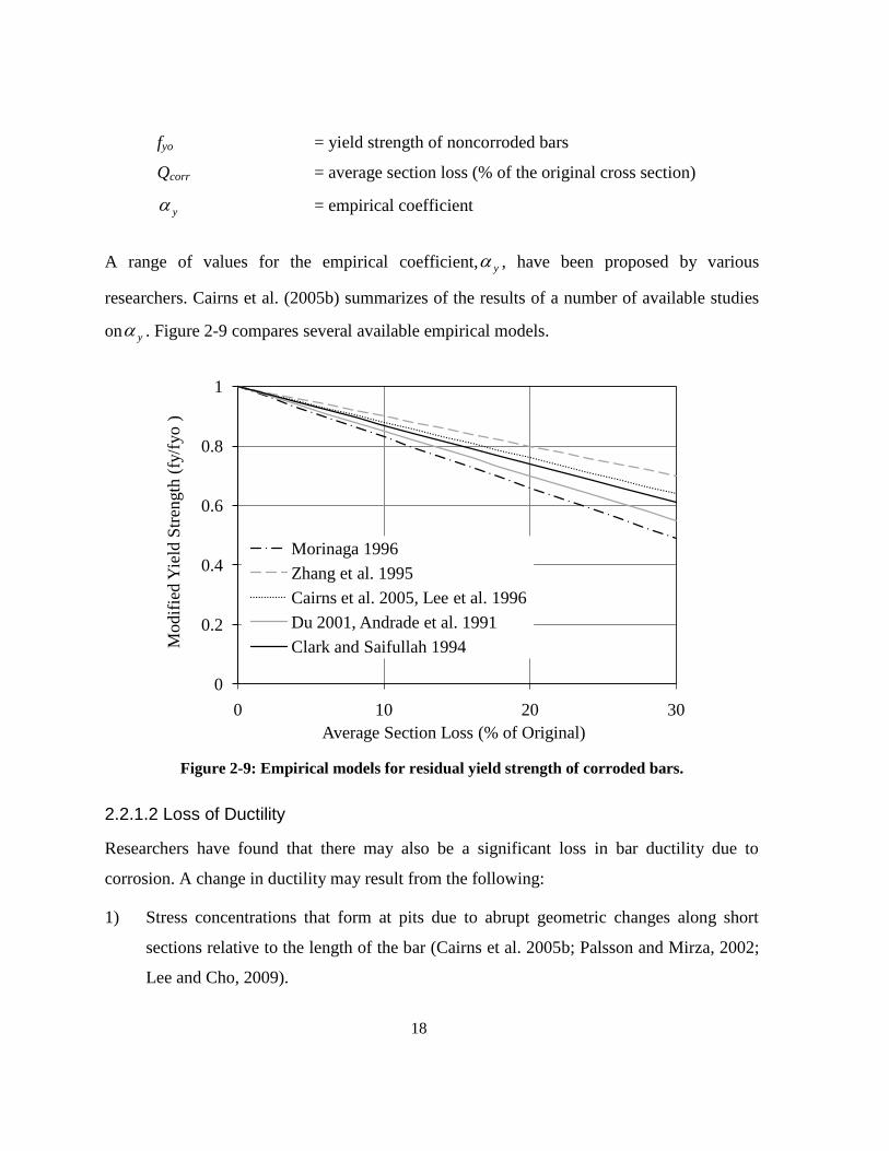
y = empirical coefficient
A range of values for the empirical coefficient, y , have been proposed by various
researchers. Cairns et al. (2005b) summarizes of the results of a number of available studies
on y . Figure 2-9 compares several available empirical models.
Figure 2-9: Empirical models for residual yield strength of corroded bars.
2.2.1.2 Loss of Ductility
Researchers have found that there may also be a significant loss in bar ductility due to
corrosion. A change in ductility may result from the following:
1) Stress concentrations that form at pits due to abrupt geometric changes along short
sections relative to the length of the bar (Cairns et al. 2005b; Palsson and Mirza, 2002;
Lee and Cho, 2009).
0
0.2
0.4
0.6
0.8
1
0 10 20 30
Modif
ied Y
ield
Str
ength
(fy
/fyo )
Average Section Loss (% of Original)
Morinaga 1996
Zhang et al. 1995
Cairns et al. 2005, Lee et al. 1996
Du 2001, Andrade et al. 1991
Clark and Saifullah 1994

19
2) Changes in the metal properties that result in a change in ductility. Palsson and Mirza
(2002), for example, found significant impurities in a spectrochemical analysis of metal
taken from an abandoned structure originally constructed in 1959.
In ageing structures, impurities are to be expected but the extent of their impact on ductility
is still unclear (Palsson and Mirza 2002) and often ignored (Cairns et al. 2005b). To consider
the change in bar ductility the following empirical relationships may be used:
1.0u u corr u0f Q f (3.9)
1.0u 1 corr 0Q (3.10)
where:
fu = ultimate tensile strength and elongation at time t
εu = elongation corresponding to the ultimate strength at time t
fuo, εuo = ultimate tensile strength and elongation of new bars
Qcorr = average section loss (% of the original cross section)
1, u = empirical coefficients
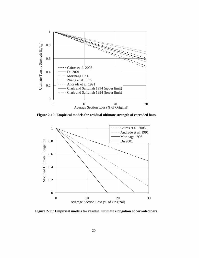
Figure 2-10 and Figure 2-11 present curves of Qcorr versus fu and εu from several studies.
20
Figure 2-10: Empirical models for residual ultimate strength of corroded bars.
Figure 2-11: Empirical models for residual ultimate elongation of corroded bars.
0
0.2
0.4
0.6
0.8
1
0 10 20 30
Ult
imat
e T
ensi
le S
tren
gth
(f u
/fu
o)
Average Section Loss (% of Original)
Cairns et al. 2005
Du 2001
Morinaga 1996
Zhang et al. 1995
Andrade et al. 1991
Clark and Saifullah 1994 (upper limit)
Clark and Saifullah 1994 (lower limit)
0
0.2
0.4
0.6
0.8
1
0 10 20 30
Mo
dif
ied U
ltim
ate
Elo
ngat
ion
Average Section Loss (% of Original)
Cairns et al. 2005
Andrade et al. 1991
Morinaga 1996
Du 2001
21
Design rules in most national standards specify a minimum ductility that should be met. The
residual ductility computed by Equations 2.9 and 2.10 must continue to satisfy these
requirements, in order to ensure adequate structural performance. On this basis, a simple
ductility check could be implemented for the evaluation of corroded structures.
2.2.2 Concrete/Steel Bond Loss
Generally, it is assumed that there are two stages of bond between concrete and steel when an
axial force is applied to a reinforcing bar cast and developed in concrete. A report on bond
(CEB 2000) describes these stages as follows: First, there exists a chemical bond between the
hardened cement and steel. This condition is generally weak and broken at low stresses. Slip
starts to occur at Stage 2; in which friction provides the bond. Where ribbed bars are used,
bearing and mechanical interlock between the ribs and surrounding concrete resists pullout.
Given that the ribs are strong, failure eventually occurs by bursting or splitting of the
surrounding concrete.
2.2.2.1 Effect of Corrosion on Bond
The effect of corrosion on bond is summarized as follows (CEB 2000):
Increased bar diameter, due to the creation of corrosion products, initially increases
radial stresses and the frictional component of bond. Bond strength increases as a
result.
When radial stresses (due to further corrosion) exceed the threshold (determined by
concrete strength and cover) bursting and splitting of the concrete cover occurs,
resulting in longitudinal cracking and a reduction in confinement and bond strength.
However, the following has also been hypothesized;
Corrosion products at the bar/concrete interface under low corrosion levels may have
a roughening effect, increasing friction and bond (Al-Sulaimani et al. 1990).
As corrosion increases, the weak corrosion product acts as a lubricant to reduce
friction and bond strength (Cabrera and Ghoddoussi 1992).
22
Under severe corrosion, bar ribs may reduce in height or fracture; reducing bearing
area and bond strength (Al-Sulaimani et al. 1990).
The layer of corrosion product may force the concrete away from the bar core and
subsequently reduce the effective rib height and bearing area; reducing bond strength.
This phenomenon is often referred to as ―disengagement of ribs‖ (CEB 2000).
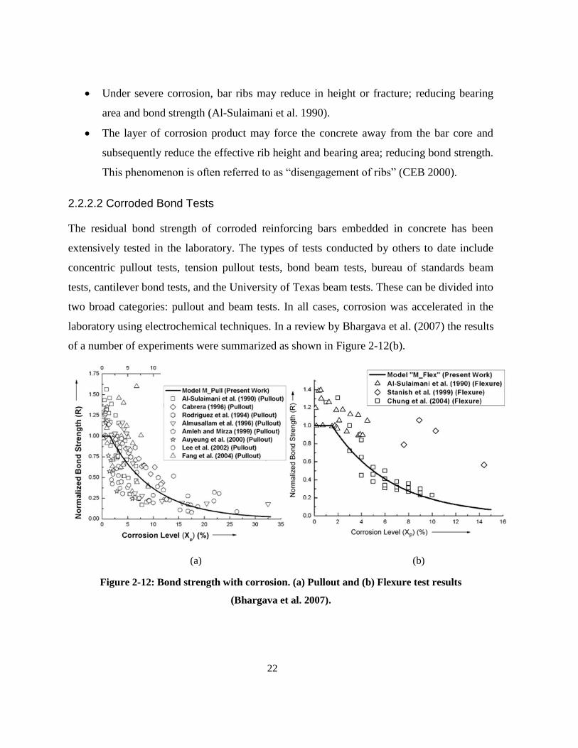
2.2.2.2 Corroded Bond Tests
The residual bond strength of corroded reinforcing bars embedded in concrete has been
extensively tested in the laboratory. The types of tests conducted by others to date include
concentric pullout tests, tension pullout tests, bond beam tests, bureau of standards beam
tests, cantilever bond tests, and the University of Texas beam tests. These can be divided into
two broad categories: pullout and beam tests. In all cases, corrosion was accelerated in the
laboratory using electrochemical techniques. In a review by Bhargava et al. (2007) the results
of a number of experiments were summarized as shown in Figure 2-12(b).
(a) (b)
Figure 2-12: Bond strength with corrosion. (a) Pullout and (b) Flexure test results
(Bhargava et al. 2007).

23
The scatter in results is obvious. Bhargava et al. (2007) attributes this variation to both the
wide-range of bond specimens and bar types tested and the variation in conditioning
techniques. The CEB/FIB report (CEB 2000) agrees that there are distinct variations in the
applied current density, methods of weight loss measurement and specimen detailing and that
―developing an appropriate measure of damage is clearly a priority in reconciling test data
and development of assessment guidelines for bond‖.
Electrochemical corrosion has limitations when compared to corrosion on real structures.
Poursee and Hansson (2009) recommend against applied anodic current corrosion
techniques, as used by the majority of researchers highlighted here, due to significant
differences between corrosion products developed artificially to those on real structures.
They suggest that the resulting corrosion is overly uniform, many tests neglect differentiating
between micro and macro cell corrosion, and specimen detailing such as steel grade and
surface finishing has variable impacts. Ballim and Reid (2002) highlight the importance of
applying the selected technique under service load levels.
2.2.2.3 Predictive models
The development of predictive models for the degradation of bond strength with corrosion is
a challenging task currently facing researchers. The influence and interaction of each of the
proposed mechanisms listed in Section 2.2.2.1 is very difficult to predict. As a result, simple
empirical and analytical relations remain as the best representations available.
Analytical Models
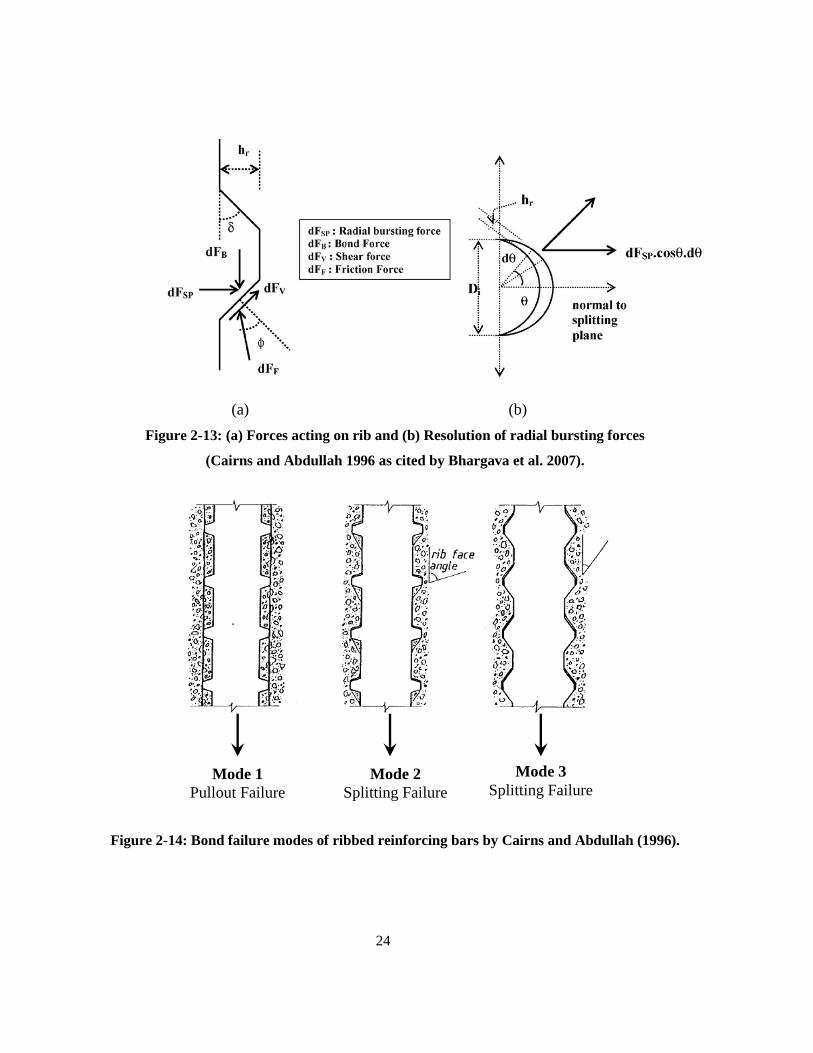
Cairns and Abdullah (1996) suggested analytical formulas to represent splitting modes of
noncorroded bar bond failure. They predicted bond strength based on the resolution of forces
acting on the ribs into radial bursting forces as shown in Figure 2-13 for failure modes 2 and
3 shown in Figure 2-14 within good agreement to laboratory test.
24
(a) (b)
Figure 2-13: (a) Forces acting on rib and (b) Resolution of radial bursting forces
(Cairns and Abdullah 1996 as cited by Bhargava et al. 2007).
Figure 2-14: Bond failure modes of ribbed reinforcing bars by Cairns and Abdullah (1996).
Mode 3
Splitting Failure Mode 2
Splitting Failure
Mode 1
Pullout Failure

25
The first mode is the standard pullout associated with concrete shear and thick cover, while
the second occurs when concrete wedges shear and no slip between rib and bearing surface
occurs. The third mode is the conventional bursting failure in which an inclined failure
surface is developed along the rib/bearing surface interface.
Coronelli (2002) expanded the model described in Figure 2-13 and Figure 2-14 to consider
corroded bars. The primary changes due to corrosion resulted in:
modified cohesion, fcoh, and angle of cohesion, φ, values,
reduced rib height, hr, values and resulting modified rib area, Ar, and
an additional pressure term, p(X), to represent the stress distribution at the
bar/concrete interface between ribs resulting from rust. The pressure is based on a
coefficient of friction for rusted steel of µ(X).
The model, correlated well with the experimental work by Rodriguez et al. (1994).
In their study, Bhargava et al. (2007) continued to modify the model by estimating
parameters such as corrosion pressure, confining action of cracked concrete and shear
stirrups after incorporating the effect of corrosion products and adhesion on friction between
steel and concrete. The modified version appears to be better for predicting, pre-cracking
behaviour but appears to add complexity.
Empirical Models
Several researchers have suggested empirical formulations to quantify bond deterioration.
Table 2.1 defines a set of conditions established (based on the case study structure) to
facilitate a comparison of the different empirical models. The comparison of available
models is shown in Figure 2-15.

26
Table 2.1: Input for bond degradation model comparison.
Input Parameter Assumed
Value Required for:
Longitudinal Bar Diameter 31.8 mm Rodriguez et al. 1994
Concrete Cover 50.8 mm Rodriguez et al. 1994
Development Length, (ld) 36.2 mm
Concrete Strength, (fc’) 20 MPa
Rodriguez et al. 1994, Chung et al. 2004
Stirrup Strength, (fy) 230 MPa Rodriguez et al. 1994
Stirrup Spacing 304.8 mm Rodriguez et al. 1994
Stirrup Area 125.7 mm2 Rodriguez et al. 1994
Figure 2-15: Empirical models for steel-concrete bond deterioration.
0
0.2
0.4
0.6
0.8
1
0 5 10 15 20 25 30
R =
Det
erio
rate
d B
ond S
tren
gth
/Init
ial
Bond S
tren
gth
Degree of Corrosion (%)
Bhargava et al. 2005 (Pullout)Chung et al. 2004 Bhargava et al. 2007 (Beam)Lee et al. 2002Rodriguez et al. 1994 (upper bound)Stanish et al. 1999Rodriguez et al. 1994 (lower bound)CONTECVET 2001 Cabrera and Ghoddoussi 1992

27
There is significant evidence in literature to suggest that a small increase or no change in
bond strength occurs at low levels of corrosion due to a slight roughening effect by the
corrosion products (Bhargava et al. 2007, Lee et al. 2002, Chung et al. 2004).
With increasing corrosion, longitudinal cracks and slip occurs and bond strength decreases
rapidly. The strength plateaus at minimal strength once confinement is lost. Simple linear
models, such as those by Stanish et al. (1999), Cabrera (1996), and the Contecvet manual
(2001), neglect these effects and appear to underestimate the bond strength at low levels of
corrosion and overestimate the strength at higher levels.
2.2.3 Composite Action
Traditional concrete design assumes that the steel is bonded perfectly to the concrete.
Tension stiffening occurs as the steel transfers tensional forces to the concrete through this
bond. Even after flexural cracking, tension stiffening continues to occur between cracks.
However, when this bond is completely compromised by corrosion, the tension stiffening
contribution of the steel is reduced or eliminated. The result is the reinforced concrete
member globally acts like a tied arch. Both flexural and shear behaviour of the member can
change. Several researchers have attempted to describe and model the change in behaviour of
beams when reinforcement is exposed. This section first develops the theory, and then
discusses the effect of a loss in composite action on flexural strength, shear strength, and
ductility.
2.2.3.1 Concept
The theoretical change in beam behaviour can be described in two stages. Stage 1 re-
equilibrates forces, while Stage 2 maintains deformation compatibility. To illustrate these
changes, first consider the normal, un-exposed beam. Equilibrium of forces is met and
deformations of the concrete and the steel are compatible. The tensile stress in the
reinforcement varies proportionally to the applied moment along the member. In the case of
symmetric point loads, as the section of interest moves towards the supports, the tensile stress
28
in the rebar and the maximum compressive stress in the concrete decrease proportional to
each other and the applied moment as shown in Figure 2-16.
Figure 2-16: Noncorroded beam subject to symmetric point loads (Cairns and Zhao 1993).
However, when bond is broken over a certain length, the tensile stress in the rebar becomes
constant along this length and equal in magnitude to the maximum experienced along this
section. To maintain equilibrium, as the applied bending moment decreases (towards the
supports) and tensile rebar stress remains constant, the lever arm must decrease. This in turn
causes the neutral axis to drop. The maximum concrete stress decreases with increased
neutral axis depth. It is possible for the neutral axis to drop to the bottom edge of the beam,
putting the entire section in compression. At very low moment sections (towards the
supports), it is even possible for a stress reversal to occur and the top fibre to be subject to
tension and the bottom fibre compression a shown in Figure 2-17.
Figure 2-17: Corroded beam after Stage 1 (Cairns and Zhao 1993).
However, in Stage 2, deformation compatibility is not satisfied. It is apparent that the
elongation in the steel reinforcement will be greater in the unbonded reinforcement due to the
constant bar strain. The extension of the bottom concrete fibre is reduced in this case. To
maintain deformation compatibility, the neutral axis depth at the midspan must be reduced as
shown in Figure 2-18. The result is higher midspan concrete compressive strains and
increased midspan curvature. Also, with a decreased depth of neutral axis, the lever arm
z
Ast
fst
Ast
fst
N.A.
x
fc f
c b(x/2)
z
29
increases, resulting in a slight decrease in the reinforcement stress. Stage 2 ends with this
stress adjustment (Cairns and Zhao 1993).
Figure 2-18: Corroded beam after Stage 2 (Cairns and Zhao 1993).
As the exposed rebar length increases, the compressive strains in the concrete also increase.
It is therefore logical that a conventionally balanced beam will become overreinforced due to
concrete crushed under reduced loads. Likewise, an underreinforced beam could fail by
concrete crushing or yielding depending on the reinforcement ratio and the length of exposed
region. Initially overreinforced members will show the most significant strength reduction,
again, due to concrete crushing occurring under reduced loads. Crushing failure is less
ductile and can occur suddenly.
2.2.3.2 Effect on Flexural Capacity
Researchers have used the following experimental research to support their hypotheses and to
verify their numerical models for predicting the effects of loss of composite action on the
behaviour of concrete beams with corroding reinforcing bars.
Laboratory Testing
Cairns and Zhao (1993) mechanically delaminated 19 test beams, to test the influence of each
of the following parameters: exposed length/span ratio, form of loading, reinforcement ratio,
and effective depth. They found underreinforced specimens, with up to 95% of the span
exposed, had no loss in strength and failure was still governed by reinforcement yielding
when anchorage was provided. On the other hand, heavily reinforced specimens, with up to
95% of their span debonded, had strengths reductions up to 50%.
z

30
To better replicate bridge girders, Bartlett (Unpublished) tested two T-beams under four
point loading, designed to fail in flexure (steel yielding). The deteriorated girder, with 50%
of its span symmetrically debonded mechanically, again attained full yield flexural strength.
Analytical Modelling
Compatibility theory and the concept discussed in Section 2.2.3.1 can be used to estimate the
flexural capacity. Cairns and Zhao (1993) proposed the method, and confirmed its validity
with a test: predicted ratio of 1.01 and a standard deviation of 0.06. They also found that the
method estimated the failure mode reasonable well and that the strains could be used to
estimate ductility. Bartlett (Unpublished) later adapted the model for application to T-beams
using CSA Standards. They reported a test to predicted ratio (test:predicted) of 1.08.
2.2.3.3 Effect on Shear Capacity
Laboratory Testing
Azam (2010) tested ten deep and ten slender shear critical beams at the University of
Waterloo, electrochemically corroding 60% and 80% of their spans respectively. They found
that the deep beams had an increase in ultimate capacity due to arch action. In these
specimens, corrosion shifted the failure from shear-compression failure to splitting of the
compression strut. The slender beams also experienced arch action, but failure shifted from
diagonal tension failure to flexure or anchorage. Similarly, Cairns and Zhao (1993) found
that shear failures did not occur in their tests, even in specimens detailed for this type of
failure. They concluded that shear strengths increased as a result of arch action and diagonal
compression fields acting as struts transfer shear stresses directly to the supports.
Analytical Modelling
Azam (2010) proposes a modified strut-and-tie model to describe the shear strength of
corroded test specimens within 15% error. For deep beams, the model checks splitting of the
struts and yielding of the tie. For slender members, they suggest that the direct strut be
replaced by an arch band.

31
2.2.3.4 Effect on Serviceability
The effects on serviceability appear to be the most significant impact due to a loss in
composite interaction. This section discusses changes in ductility and issues regarding
cracking.
Ductility
Cairns and Zhao (1993) found, as expected, that reinforcement strains at failure do indicate
an overall loss of ductility due to the loss of composite action. Bartlett (Unpublished) noted
that their test specimen had an 80% reduction in ultimate moment capacity and flexural
stiffness. The analytical model suggested in Section 2.2.3.2 is capable of determining
ductility changes. As expected, Azam (2010) found that shear sensitive beams also
experienced a reduction in ductility and increased deflections.
Cracking
Deflections and cracking becomes more severe with the loss of composite interaction. Cairns
and Zhao (1993) noted that in members where concrete crushing governed, large cracks at a
wide spacing appeared under low loads in the constant moment zones. These cracks extended
to the level of the neutral axis, often propagating outwards under increased loading. Near the
supports, cracks developed in the top flange, where it was evident that tension was present, as
anticipated, and curvature was significant. They also found that crushing of concrete at the
ends of the exposed regions on the tension face occurred if they intersected the inclined
compressive struts.
2.3 Summary
The majority of the existing research on each of the effects of corrosion on the remaining
structural capacity of reinforced concrete flexural members has focused on exclusively
considering one or several of the effects in isolation. In the case of the laboratory tests, none
of the cited studies have modelled the effects of spalling in the vicinity of lap splices or bar

32
ends. In all cases bars are fully developed into supports. As a result, there currently exists
little in the way of previous research examining the interactions of these corrosion effects and
how they may influence the remaining structural capacities of real, heavily spalled bridge
girders. On this basis, a ―modified area concept‖, which offers a practical way of considering
these affects, is proposed, developed, and then demonstrated on a case study bridge in the
following chapters.
33
Chapter 3
Structural Strength Assessment
3.1 Introduction
It is apparent that reinforced concrete structures retain their structural capacity and function
after significant spalling has occurred. In fact, aging bridge infrastructure in Canada remains
in service and appears to be performing adequately despite obvious extensive deterioration.
The commonly adopted explanation is arch action and the development of inclined
compressive struts as discussed in Section 2.2.3. Bar development, however, becomes critical
when tension ties form and many studies assume that bars are sufficiently developed and
development regions are completely undeteriorated. In reality, this is not the case. Spalling
may occur randomly along the span of a bridge, and reinforcing splices are common in
structures of aging vintage. The potential bond failure is brittle, sudden, and potentially
catastrophic. The concepts developed in this chapter provide a simple structural analysis tool,
capable of evaluating a structure‘s capacity and reliability given any spalling pattern and
severity and the positioning of reinforcement curtailment. This chapter uses a case study
structure presented in Section 3.2, to develop the modified area concept introduced in Section
3.3. The concept is applied to proportionally reduce flexural and shear capacities in Sections
3.4 and 3.5 respectively. Finally, Section 3.5 presents a simple reliability study based on the
CAN/CSA S6-06 bridge evaluation procedures to provide early indications of individual
girder and overall bridge deficiencies created by exposed reinforcement.
3.2 Case Study Structure
The case study structure provided by the MTO represents a typical structure of concern. It
was indicated by Ministry engineers that there are currently a large number of structures of
the same design and vintage currently in service in Ontario along 400 series highways.
Therefore, this structure was used to develop the concept and analysis program. This section
discusses the background, deterioration, and the available resources for this structure.

34
3.2.1 Background
The case study structure crosses a major highway with an annual average daily traffic
(AADT) of more than 425,000 vehicles. Originally designed in May 1954, the structure is a
single span, conventionally reinforced slab on girder rigid frame as shown in Figure 3-1.
Although it is shaped as an arch, design details indicate that this feature is simply for
aesthetics and an increased shear capacity at critical locations. In service, the structure
supports two lanes of traffic while spanning six lanes of highway at a skew angle of 107°.
Ministry engineers have indicated that the narrow shoulders would not be sufficient for
future highway expansions that may be inevitable. When these occur, a full bridge
replacement will be necessary.
Figure 3-1: Case study structure (a) Cross section, and (b) Elevation.
The flexural reinforcing consists of a bottom lower level with bottom upper reinforcement in
the maximum positive moment regions. Negative moment top steel spans the length of the
structure, with a second (lower) layer in the maximum negative moment regions. The
flexural reinforcing bars are spliced with butt or lap splices as shown in Appendix A-1.
HALF SECTION ELEVATION
CROSS SECTION
HALF SECTION ELEVATION
CROSS SECTION(a)
(b)

35
3.2.2 Deterioration
The structure has been under investigation by the Ministry for several years. In 1991,
Shotcrete repairs were performed to address concerns of spalling and delamination on the
girder soffits. Drawings specifying the details of these repairs were provided by the Ministry.
To gauge the success of the repairs, the current spalling pattern was superimposed on the
drawing specifying the repair details as shown in Appendix A-3. It was concluded from this
qualitative analysis that the current spalling is randomly distributed with little or no
correlation to the previous repairs. Significant deterioration of the structure is evident by site
inspection and photographs. The visible deterioration includes:
hand rail corrosion, rust holes and staining of adjacent concrete,
exposure of rail support bolts and sidewalk deterioration,
leakage and staining below expansion joints,
girder soffit spalling and delamination exposing the bottom layer of reinforcing steel,
staining and spalling below stirrups on girder soffits, and
minor slab soffit spalling.
Of these deterioration effects, the severe spalling and delamination of the girder soffits as
shown in Figure 3-2, poses the greatest threat to the ultimate strength of the structure and
therefore is the primary concern of the current investigation and research.
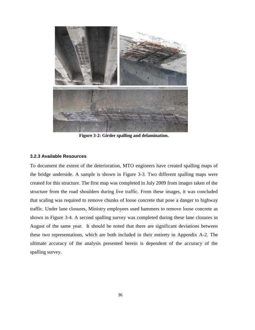
36
Figure 3-2: Girder spalling and delamination.
3.2.3 Available Resources
To document the extent of the deterioration, MTO engineers have created spalling maps of
the bridge underside. A sample is shown in Figure 3-3. Two different spalling maps were
created for this structure. The first map was completed in July 2009 from images taken of the
structure from the road shoulders during live traffic. From these images, it was concluded
that scaling was required to remove chunks of loose concrete that pose a danger to highway
traffic. Under lane closures, Ministry employees used hammers to remove loose concrete as
shown in Figure 3-4. A second spalling survey was completed during these lane closures in
August of the same year. It should be noted that there are significant deviations between
these two representations, which are both included in their entirety in Appendix A-2. The
ultimate accuracy of the analysis presented herein is dependent of the accuracy of the
spalling survey.
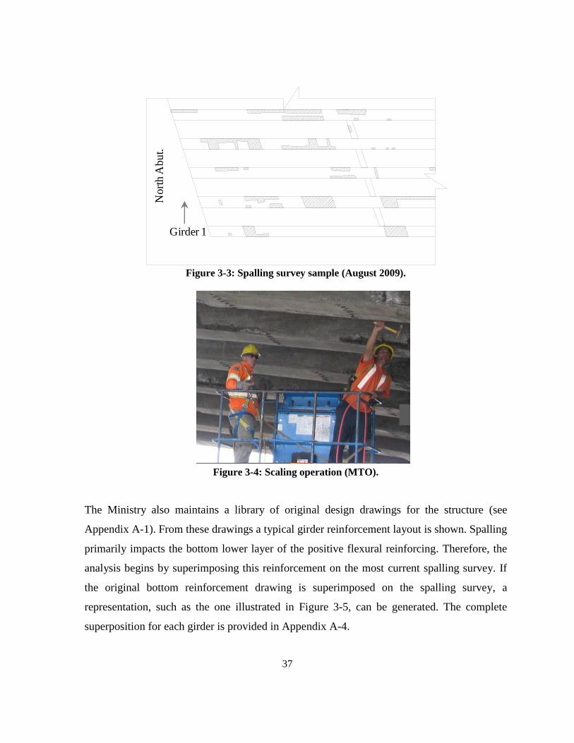
37
Figure 3-3: Spalling survey sample (August 2009).
Figure 3-4: Scaling operation (MTO).
The Ministry also maintains a library of original design drawings for the structure (see
Appendix A-1). From these drawings a typical girder reinforcement layout is shown. Spalling
primarily impacts the bottom lower layer of the positive flexural reinforcing. Therefore, the
analysis begins by superimposing this reinforcement on the most current spalling survey. If
the original bottom reinforcement drawing is superimposed on the spalling survey, a
representation, such as the one illustrated in Figure 3-5, can be generated. The complete
superposition for each girder is provided in Appendix A-4.
No
rth
Ab
ut.
Girder 1
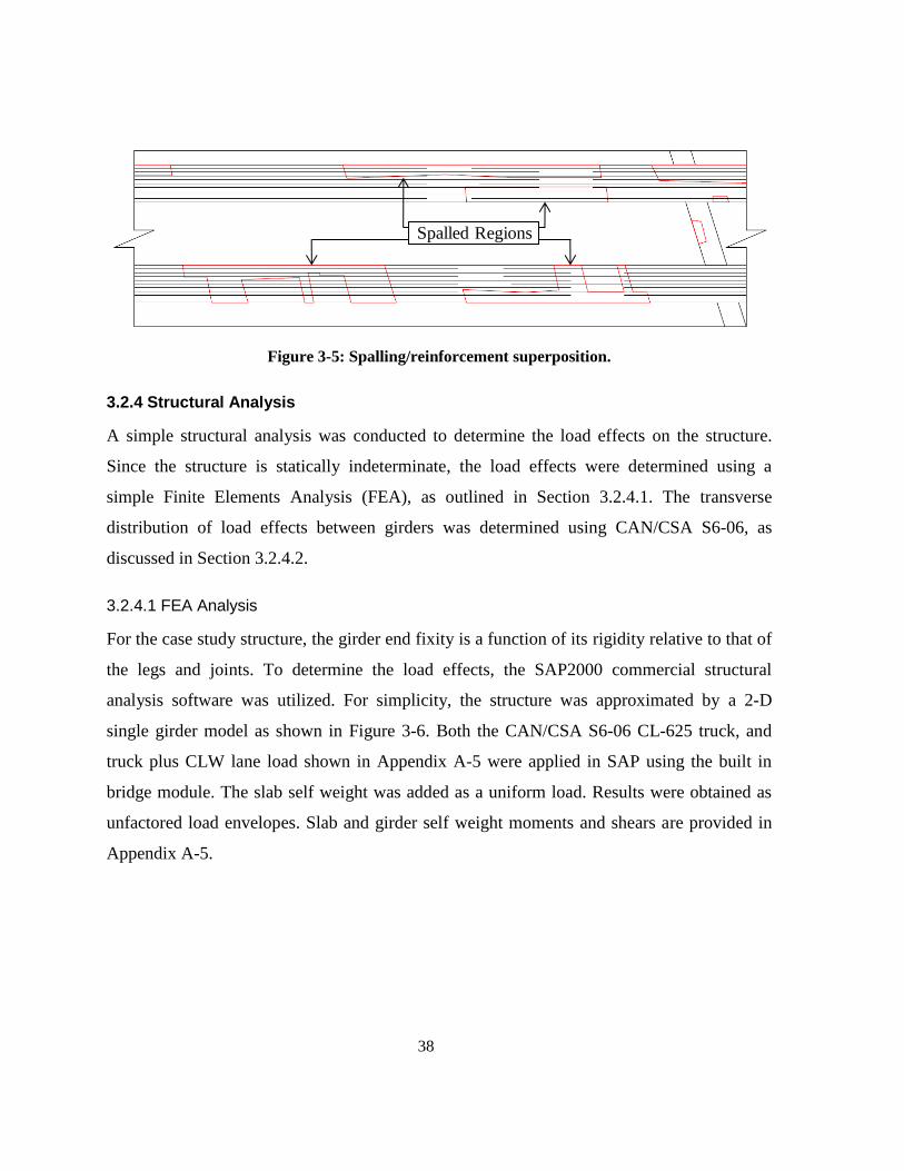
38
Figure 3-5: Spalling/reinforcement superposition.
3.2.4 Structural Analysis
A simple structural analysis was conducted to determine the load effects on the structure.
Since the structure is statically indeterminate, the load effects were determined using a
simple Finite Elements Analysis (FEA), as outlined in Section 3.2.4.1. The transverse
distribution of load effects between girders was determined using CAN/CSA S6-06, as
discussed in Section 3.2.4.2.
3.2.4.1 FEA Analysis
For the case study structure, the girder end fixity is a function of its rigidity relative to that of
the legs and joints. To determine the load effects, the SAP2000 commercial structural
analysis software was utilized. For simplicity, the structure was approximated by a 2-D
single girder model as shown in Figure 3-6. Both the CAN/CSA S6-06 CL-625 truck, and
truck plus CLW lane load shown in Appendix A-5 were applied in SAP using the built in
bridge module. The slab self weight was added as a uniform load. Results were obtained as
unfactored load envelopes. Slab and girder self weight moments and shears are provided in
Appendix A-5.
Spalled Regions
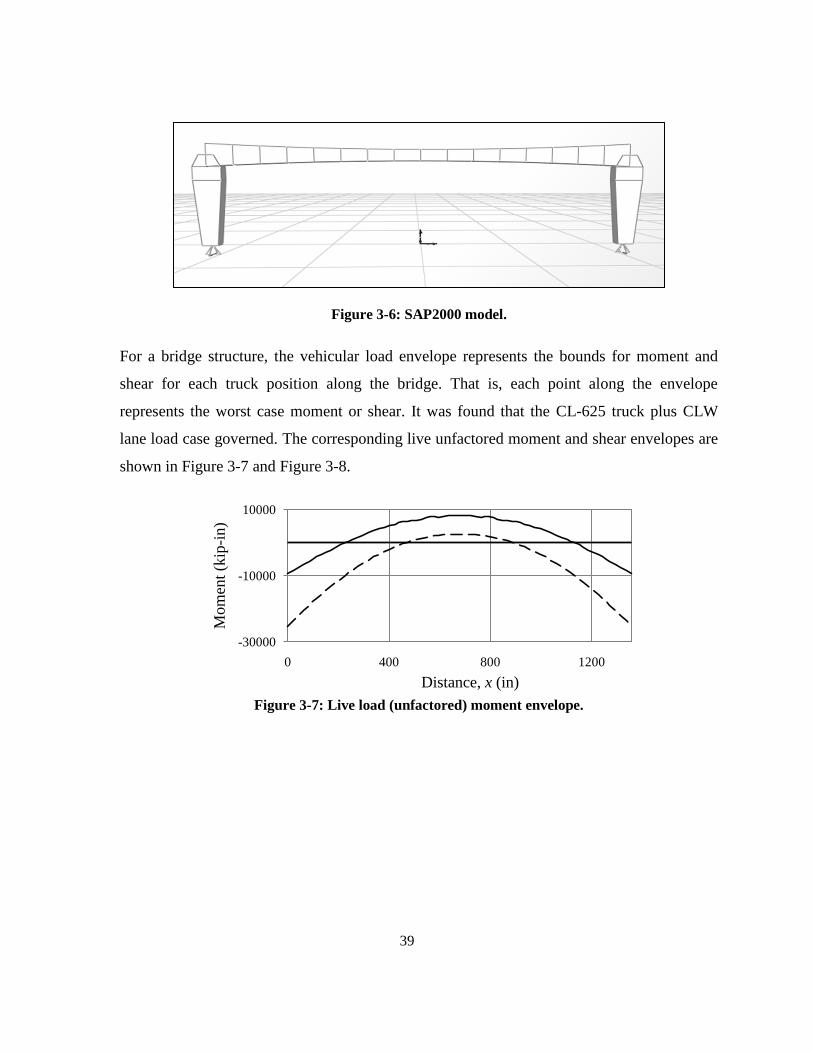
39
-30000
-10000
10000
0 400 800 1200
Mom
ent
(kip
-in)
Distance, x (in)
Figure 3-6: SAP2000 model.
For a bridge structure, the vehicular load envelope represents the bounds for moment and
shear for each truck position along the bridge. That is, each point along the envelope
represents the worst case moment or shear. It was found that the CL-625 truck plus CLW
lane load case governed. The corresponding live unfactored moment and shear envelopes are
shown in Figure 3-7 and Figure 3-8.
Figure 3-7: Live load (unfactored) moment envelope.
Figure 3.5 Sap 2000 Model

40
-100
-50
0
50
100
0 400 800 1200
Sh
ear
(kip
)
Distance, x (in)
Figure 3-8: Live load (unfactored) shear envelope.
3.2.4.2 Transverse Distribution
In lieu of a time consuming 3-D analysis, the CAN/CSA S6-06 simplified transverse
distribution model was used. Simplified live load analysis may be used if all the criteria of
Cl. 5.7.1.1 of this standard are met. The approach provides amplification factors for the (2-D)
beam analogy method. These transverse distribution factors are computed in Appendix A-7.
3.3 Modified Strength Concept
For the investigated bridge, a typical longitudinal reinforcing bar is spliced 3-4 times along
the length of the girder. At each splice location, development can be compromised by the
spalling. Upon examination of the spalling surveys in Appendix A-4, it was noted that
several longitudinal bars end in spalled regions or have significant spalling along their length.
Therefore, the proposed concept evaluates the residual strength due to development
deficiencies resulting from spalling. The modified area concept is founded on the following
basic assumptions:
1) The spalled areas are fully de-bonded with no remaining force transfer.
2) Full concrete and bond strength is assumed in the unspalled areas.

41
3) The reinforcing steel is at full strength and has no change in strength or ductility due
to corrosion.
4) The bond strength is linearly proportional to the available development length.
Each of these assumptions is addressed later in this thesis in subsequent refinements of the
model. The following sections introduce CAN/CSA A23.3-04 development, moment and
shear design concepts and use each to determine modified moment and shear capacities for
any member with exposed reinforcement.
3.3.1 CSA Development Length
CAN/CSA A23.3-04 considers development secondary to flexural design. Bars are simply
designed to ensure that development and splice lengths are ―sufficiently over-strengthened to
decrease the probability of a bond related failure before failure occurs in a more ductile
flexure mode‖. For bars in tension, CAN/CSA S6-06 defines the required development
length, ld , as follows,
S6-06, Cl. 8.15.2.2 1 2 30.45
( )
y
d b
tr cs cr
fk k kl A
k d f
(3.11)
S6-06, Cl. 8.15.2.2 0.4510.5
tr y
tr
A fk
s n (3.12)
where:
k1k2k3 = modification factors for the effects of casting position, epoxy coating and
bar size
dcs = the lesser of 2/3 bar diameter or distance from bar to closest concrete
surface
Ab = x-sectional area of the bar being developed
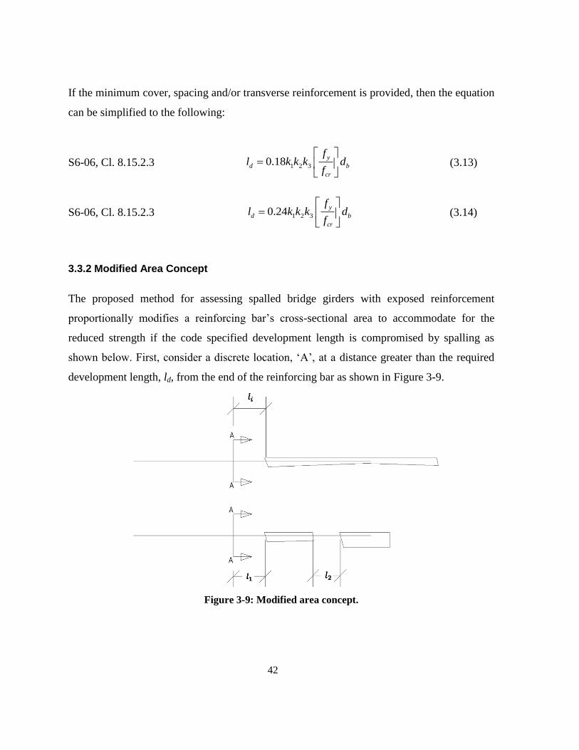
42
If the minimum cover, spacing and/or transverse reinforcement is provided, then the equation
can be simplified to the following:
S6-06, Cl. 8.15.2.3 1 2 30.18y
d b
cr
fl k k k d
f
(3.13)
S6-06, Cl. 8.15.2.3 1 2 30.24y
d b
cr
fl k k k d
f
(3.14)
3.3.2 Modified Area Concept
The proposed method for assessing spalled bridge girders with exposed reinforcement
proportionally modifies a reinforcing bar‘s cross-sectional area to accommodate for the
reduced strength if the code specified development length is compromised by spalling as
shown below. First, consider a discrete location, ‗A‘, at a distance greater than the required
development length, ld, from the end of the reinforcing bar as shown in Figure 3-9.
Figure 3-9: Modified area concept.
43
At Section ‗A‘ the remaining intact length available for development is li. If multiple spalled
regions are present, then the intact length is simply taken as the sum of each intact section,
i.e.:
1
n
i k
k
l l
(3.15)
If the intact length is less than the required development length (i.e. li < ld), then the proposed
method proportionally modifies the bar‘s cross-sectional area as follows:
' id d
d
lA A
l
(3.16)
where:
li = intact (remaining) length
Ad = actual (unspalled) bar cross sectional area
Ad’ = modified bar cross sectional area
If the intact length is greater than the required development length (i.e. li > ld), then the bar
area is not modified.
3.4 Modified Moment Resistance
The flexural capacity of a reinforced concrete member is a function of:
1. concrete strength
2. steel strength
3. sectional geometry
4. development length
If the development length is compromised, then the flexural capacity is reduced. This section
describes this concept, after introducing the CAN/CSA A23.3-04 provisions for moment
capacity.
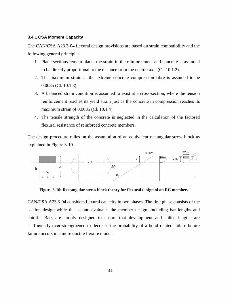
44
3.4.1 CSA Moment Capacity
The CAN/CSA A23.3-04 flexural design provisions are based on strain compatibility and the
following general principles:
1. Plane sections remain plane: the strain in the reinforcement and concrete is assumed
to be directly proportional to the distance from the neutral axis (Cl. 10.1.2).
2. The maximum strain at the extreme concrete compression fibre is assumed to be
0.0035 (Cl. 10.1.3).
3. A balanced strain condition is assumed to exist at a cross-section, where the tension
reinforcement reaches its yield strain just as the concrete in compression reaches its
maximum strain of 0.0035 (Cl. 10.1.4).
4. The tensile strength of the concrete is neglected in the calculation of the factored
flexural resistance of reinforced concrete members.
The design procedure relies on the assumption of an equivalent rectangular stress block as
explained in Figure 3-10.
Figure 3-10: Rectangular stress block theory for flexural design of an RC member.
CAN/CSA A23.3-04 considers flexural capacity in two phases. The first phase consists of the
section design while the second evaluates the member design, including bar lengths and
cutoffs. Bars are simply designed to ensure that development and splice lengths are
―sufficiently over-strengthened to decrease the probability of a bond related failure before
failure occurs in a more ductile flexure mode‖.
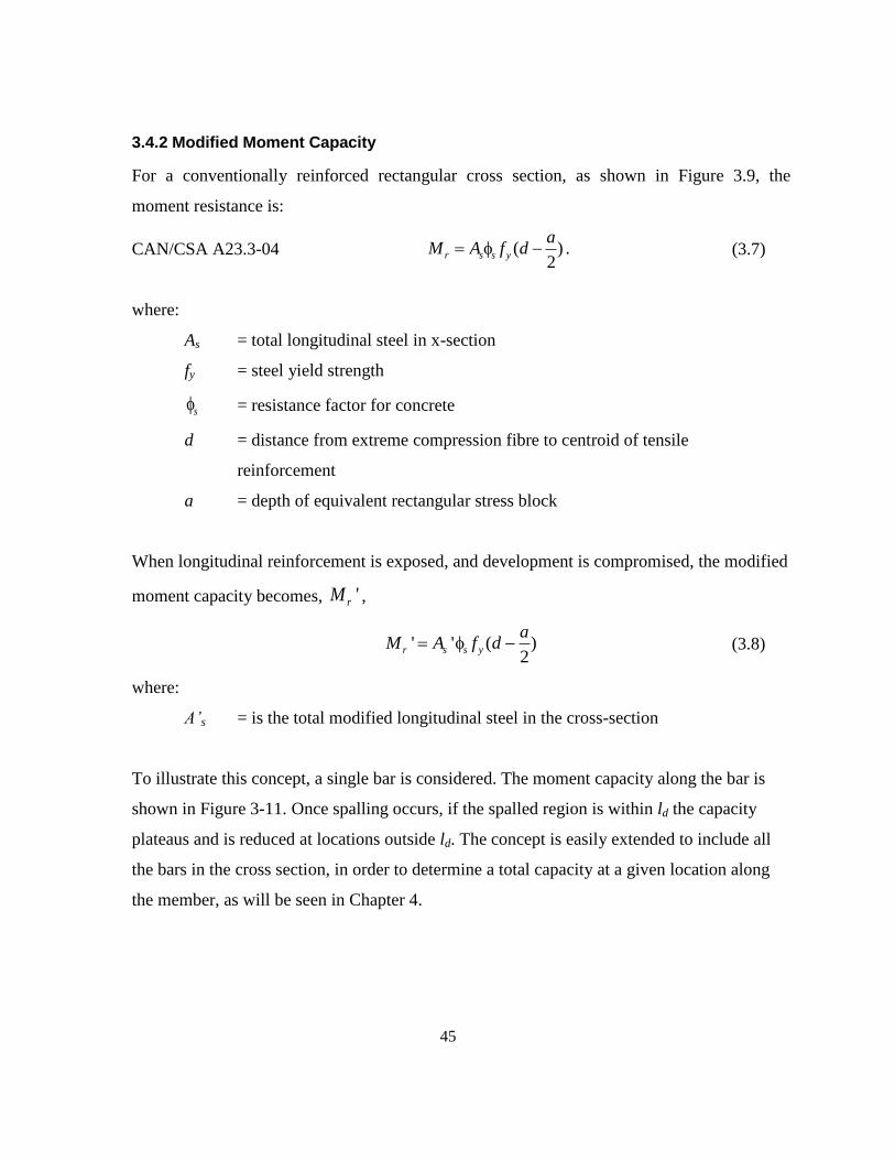
45
3.4.2 Modified Moment Capacity
For a conventionally reinforced rectangular cross section, as shown in Figure 3.9, the
moment resistance is:
CAN/CSA A23.3-04 ( )2
r s s y
aM A f d . (3.7)
where:
As = total longitudinal steel in x-section
fy = steel yield strength
s = resistance factor for concrete
d = distance from extreme compression fibre to centroid of tensile
reinforcement
a = depth of equivalent rectangular stress block
When longitudinal reinforcement is exposed, and development is compromised, the modified
moment capacity becomes, 'rM ,
' (' )2
r s s y
aM A f d (3.8)
where:
A’s = is the total modified longitudinal steel in the cross-section
To illustrate this concept, a single bar is considered. The moment capacity along the bar is
shown in Figure 3-11. Once spalling occurs, if the spalled region is within ld the capacity
plateaus and is reduced at locations outside ld. The concept is easily extended to include all
the bars in the cross section, in order to determine a total capacity at a given location along
the member, as will be seen in Chapter 4.
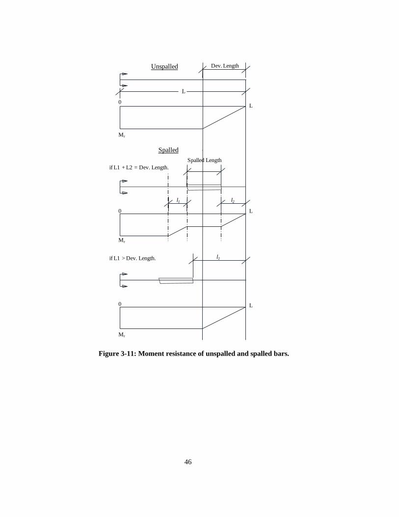
46
Figure 3-11: Moment resistance of unspalled and spalled bars.
Mr
Mr
Mr
0
0
0
Dev. Length
L
L
L
L
Spalled Length
Unspalled
Spalled
l2l1
l1
if L1 + L2 = Dev. Length.
if L1 > Dev. Length.
.
.

47
3.5 Modified Shear Resistance
Exposing longitudinal reinforcement (spalling), also has an adverse effect on the shear
capacity of a reinforced concrete member, if the development of longitudinal reinforcement
is compromised. Although longitudinal reinforcing is primarily specified for moment and
axial loads, the shear force on an inclined shear crack has both vertical and horizontal
components as shown in Figure 3-12. The horizontal component must be resisted by the
longitudinal reinforcement, and subsequently the longitudinal reinforcement anchorage.
Figure 3-12: Basic shear resisting mechanism assumed by Bentz (2006).
The proposed approach for shear assessment assumes that:
stirrups (transverse reinforcing) are undeteriorated with no loss in strength due to
corrosion, and
the interaction between longitudinal and transverse reinforcement is
uncompromised.
The following sections first introduce the CAN/CSA A23.3-04 shear design provisions in
3.5.1 and then recommend two methods for determining the shear capacity of a spalled girder
analogous with the CAN/CSA A23.3-04 ―simplified‖ and ―general‖ methods (Cl. 3.5.2 and
3.5.3).
48
3.5.1 CSA Shear Capacity
Canadian design codes allow designers to use either of two methods for computing the shear
capacity of a reinforced concrete member. In both cases, the shear resistance is a combination
of contributions from both the concrete and steel, as defined below:
S6-06, Cl. 8.9.3.4 2.5 c cr v vV f b d (3.9)
S6-06, Cl. 8.9.3.5 cots v y v
s
A f dV
s
(3.10)
S6-06, Cl. 8.9.3.3 r c sV V V (3.11)
The General Method, is based on the modified compression field theory. Canadian standards
provide simple formulae for computing the size and strain effects that contribute to the
computation of Vc and Vs . The parameter characterizing aggregate interlocking on cracked
concrete, , is defined as:
A23.3, Cl. 11.3.6.4 0.40 1300
(1 1500 ) (1000 )x ZES
(3.12)
The strain effect is characterized by the average longitudinal strain in a member at mid-
depth, which can be estimated according to the following relationship:
A23.3, Cl. 11.3.6.4
2
f
f
vx
s s
MV
d
E A
(3.13)
The angle of inclination of the diagonal compressive stress is based on the strain effect as
follows:
A23.3, Cl. 11.3.6.4 29 7000 x (3.14)
49
Design codes are structured for easy design and as a result the method becomes iterative for
evaluation. As an alternative, the code also provides a Simplified Method. This method treats
the mid-depth strain as constrained. If the yield strain for steel is 0.002, any mid-depth
strains greater than half of 0.002 would result in flexural failure. Therefore, the mid-depth
strain should be less than 0.001. The Simplified Method considers the upper bound to be:
S6-06, Cl. 8.9.3.6 30.8 10x
A23.3, Cl. 8.9.3.6 30.85 10x
If these are applied to Equation 3.14 and Equation 3.12 then:
S6-06, Cl. 8.9.3.6 42
S6-06, Cl. 8.9.3.6 0.18
The method is both simple and conservative. For the evaluation of a spalled concrete girder,
two methods have been derived analogous to the CSA A23.3 Simplified and General
methods.
3.5.2 Modified Shear Capacity based on CSA Simplified Method
Theoretically, for both the deteriorated and undeteriorated cases, a first assumption can be
made that the applied load effects and material properties do not change as the result of
spalling. To consider spalling, the modified area concept can also be applied for the shear
verification. If we consider the change in mid–depth strain due to bond loss, x can be
modified to 'x for the spalled case as follows:
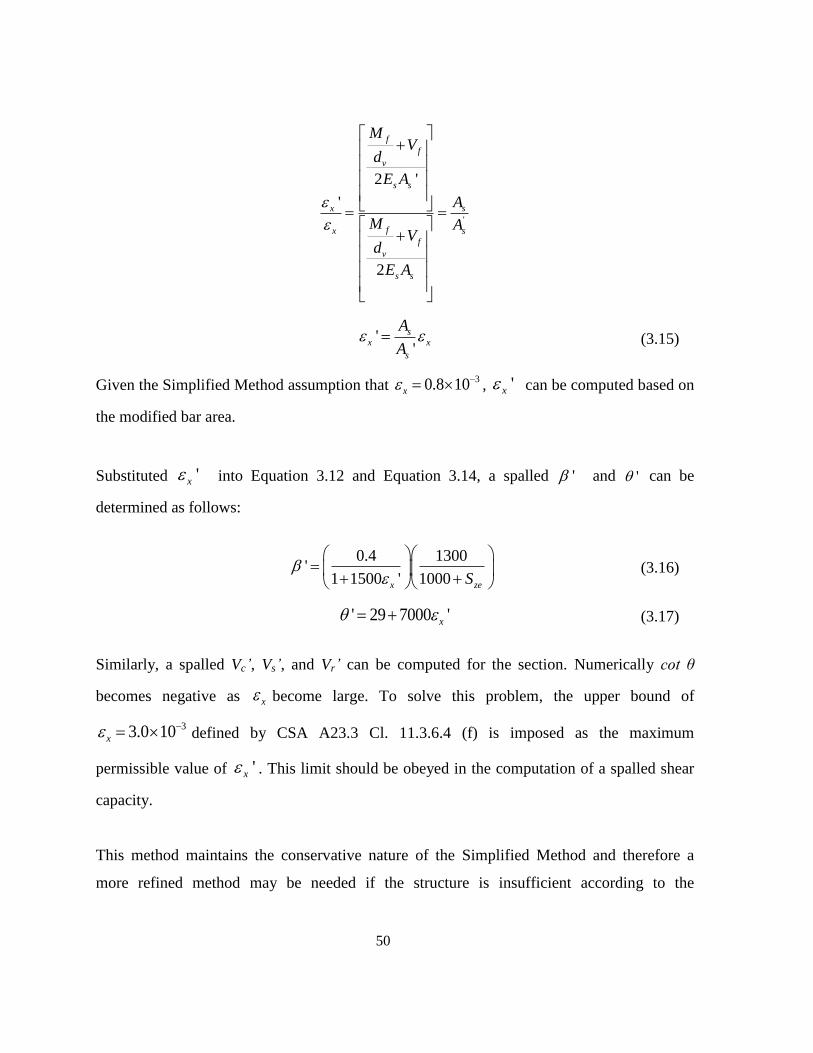
50
'
2 '
'
2
f
f
v
s s
x s
fx s
f
v
s s
MV
d
E A
A
M AV
d
E A
' ' s
x x
s
A
A (3.15)
Given the Simplified Method assumption that 30.8 10x , 'x can be computed based on
the modified bar area.
Substituted 'x into Equation 3.12 and Equation 3.14, a spalled ' and ' can be
determined as follows:
0.4 1300
' 1 1500 10' 00x zeS
(3.16)
' 29 7000 'x (3.17)
Similarly, a spalled Vc’, Vs’, and Vr’ can be computed for the section. Numerically cot θ
becomes negative as x become large. To solve this problem, the upper bound of
33.0 1 0x defined by CSA A23.3 Cl. 11.3.6.4 (f) is imposed as the maximum
permissible value of 'x . This limit should be obeyed in the computation of a spalled shear
capacity.
This method maintains the conservative nature of the Simplified Method and therefore a
more refined method may be needed if the structure is insufficient according to the

51
Simplified Method. Section 3.5.3 discusses the development of a General Method for
evaluation.
3.5.3 Modified Shear Capacity based on CSA General Method
The direct application of the General Method for the case study structure is not a straight
forward task. Since the structure is statically indeterminate and subject to a moving
(vehicular) load, at a given section along the span of the structure, factored moment and
shear (Mf and Vf ) combinations need to be checked for each position of the code truck along
the span. In general, the code truck positions that cause the maximum values of Mf and Vf
will not be the same. The computation of εx for the application of the General Method at each
section along the structure subject to a large number of load effect combinations (i.e. for each
truck position) can thus be a very time-consuming task. As a simple approximation, the
largest absolute factored moment and shear may be combined to determine εx for the purpose
of calculating the shear resistance. That is, although the worst case moment and shear may
not coincide with the same truck position, using a combination of the two extreme values will
result in a conservative assessment. The maximum shear and moment for each position
along the structure can be taken from the moving load envelopes shown previously in Figure
3.6 and 3.7.
Once the factored moment and shear values are selected, they can be used to calculate the
mid-depth strain as follows:
'
2 '
f
f
v
x
s s
MV
d
E A
(3.18)
To determine the resistance, Equations 3.16 and 3.17 can be used along with the modified
area concept. Chapter 4 discusses the application of this concept in a computer program and
presents the assessment results when applied to the case study structure.
52
3.6 Reliability Analysis
Even though significant reductions in strength may occur when a structural component is
subject to deterioration, the structural performance of the component may still be adequate.
This section provides an approximate means for estimating the remaining reliability of
deteriorating structural components and full bridge structures deterministically. First, the
reliability index concept is introduced and its application to bridge evaluation according to
CAN/CSA S6-06 is described. Based on this concept of structural evaluation, an approximate
reliability method is proposed to determine the reliability index for each individual girder.
Following this, the concept is expanded to allow the estimation of a reliability index for the
entire structure.
3.6.1 CSA Target Reliability Index
The philosophy behind structural evaluation according to CAN/CSA S6-06 is to maintain a
consistent level of risk of loss of human life for each structural element of a bridge. However,
structures that experience regular inspection, show warning before failure, and can
redistribute loads to other elements, have a reduced probability of loss of life in the event of
failure compared to those that do not exhibit these traits. A consistent level of risk is
maintained by a combination of the probability and consequence of failure as shown in
Figure 3-13 (Figure C14.1 in CAN/CSA S6-06).

53
Figure 3-13: Relationship between risk and reliability (CAN/CSA S6-06).
CAN/CSA S6-06 bridge evaluation categorizes the target reliability index based on the
system and element behaviour and the level of inspection. Each are described below.
Table 3.1: System behaviour (CAN/CSA S6-06).
Category Description
S1 Element failure leads to total collapse.
S2 Element failure probably will not lead to total collapse.
S3 Element failure leads to local failure only.
Table 3.2: Element behaviour (CAN/CSA S6-06).
Category Description
E1 Element being considered is subject to sudden loss of capacity with little or no
warning.
E2 Element being considered is subject to sudden failure with little or no warning
but will retain post-failure capacity.
E3 Element being considered is subject to gradual failure with warning of probable
failure.
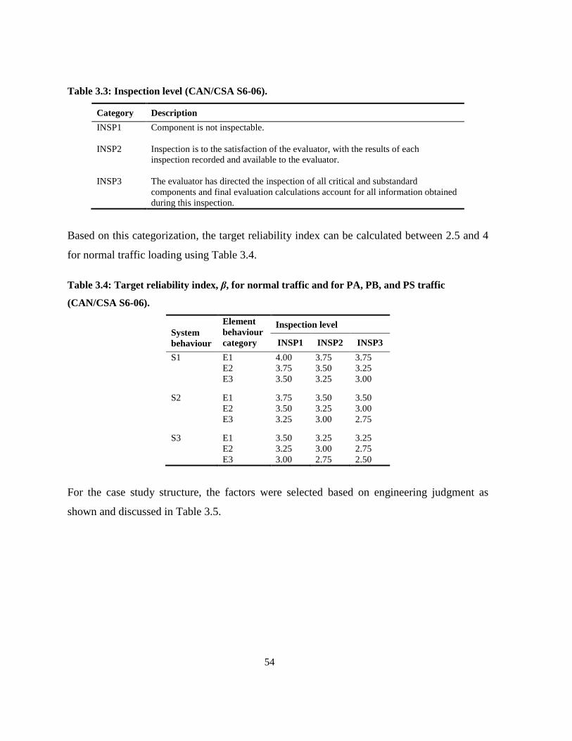
54
Table 3.3: Inspection level (CAN/CSA S6-06).
Category Description
INSP1 Component is not inspectable.
INSP2 Inspection is to the satisfaction of the evaluator, with the results of each
inspection recorded and available to the evaluator.
INSP3 The evaluator has directed the inspection of all critical and substandard
components and final evaluation calculations account for all information obtained
during this inspection.
Based on this categorization, the target reliability index can be calculated between 2.5 and 4
for normal traffic loading using Table 3.4.
Table 3.4: Target reliability index, β, for normal traffic and for PA, PB, and PS traffic
(CAN/CSA S6-06).
System
behaviour
category
Element
behaviour
category
Inspection level
INSP1 INSP2 INSP3
S1 E1 4.00 3.75 3.75
E2 3.75 3.50 3.25
E3 3.50 3.25 3.00
S2 E1 3.75 3.50 3.50
E2 3.50 3.25 3.00
E3 3.25 3.00 2.75
S3 E1 3.50 3.25 3.25
E2 3.25 3.00 2.75
E3 3.00 2.75 2.50
For the case study structure, the factors were selected based on engineering judgment as
shown and discussed in Table 3.5.

55
Table 3.5: Reliability index factors for the case study structure.
Component Category Discussion
Traffic Normal Traffic designated as Normal.
System Behaviour S2 The strength of the slab indicates that element failure
probably will not lead to total collapse.
Element Behaviour E1 Anchorage failure is sudden without warning or post-
failure capacity.
Inspection Level INSP2 Inspection conditions are satisfactory but not ideal.
On this basis, a target reliability index of 3.5 was selected from Table 3.4 for this structure.
3.6.2 CSA Reliability Evaluation
CAN/CSA S6-06 specifies modified load factors for the evaluation of existing structures at
any given target reliability index. The load factors are separated for the live load and dead
load components, which are defined in Table 3.6.
Table 3.6: Dead load components for evaluation (CAN/CSA S6-06).
Category Description
D1 Dead load of factory-produced components and cast-in-place concrete, excluding
decks.
D2 Cast-in-place concrete decks, wood, field-measured bituminous surfacing, and
non-structural components.
D3 Bituminous surfacing where the nominal thickness is assumed to be 90mm for
the evaluation.
Table 3.7 and Table 3.8 provide load factors to be used for evaluation based on the desired
reliability index.
Table 3.7: Maximum dead load factors, D (CAN/CSA S6-06).
Target reliability index,
Dead load category 2.00 2.25 2.50 2.75 3.00 3.25 3.50 3.75 4.00
D1 1.03 1.04 1.05 1.06 1.07 1.08 1.09 1.10 1.11
D2 2.06 1.08 1.10 1.12 1.14 1.16 1.18 1.20 1.22
D3 1.15 1.20 1.25 1.30 1.35 1.40 1.45 1.50 1.55
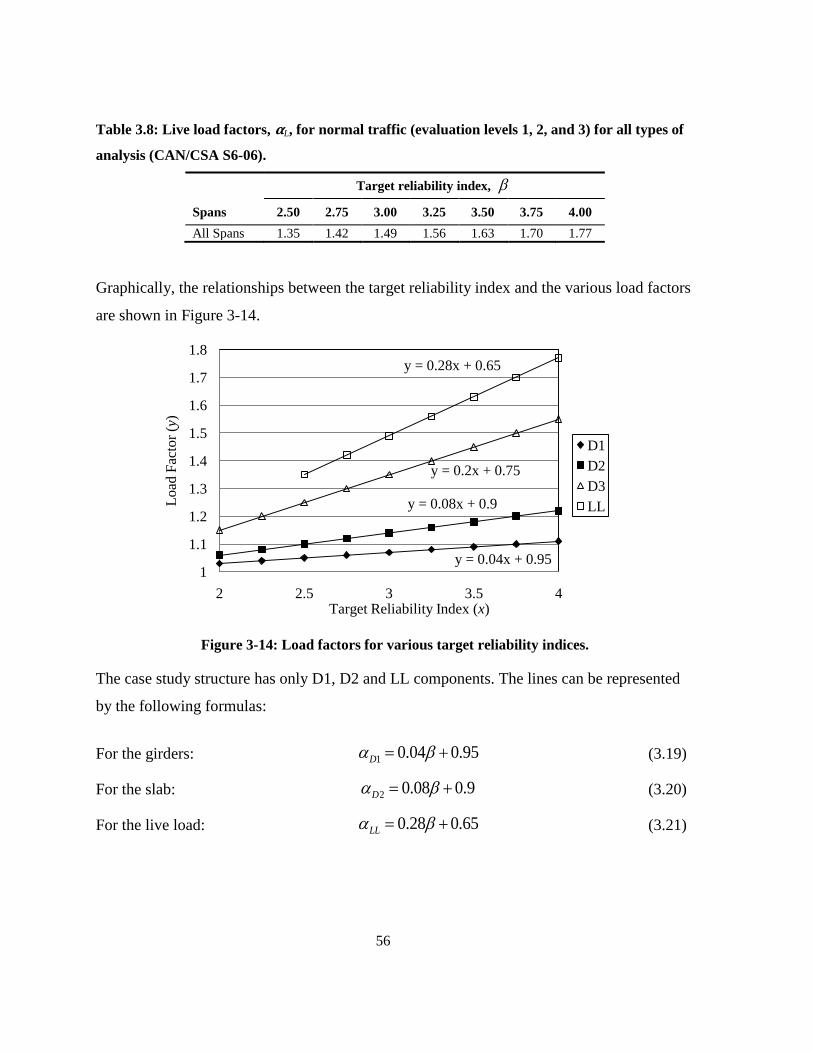
56
Table 3.8: Live load factors, L, for normal traffic (evaluation levels 1, 2, and 3) for all types of
analysis (CAN/CSA S6-06).
Target reliability index,
Spans 2.50 2.75 3.00 3.25 3.50 3.75 4.00
All Spans 1.35 1.42 1.49 1.56 1.63 1.70 1.77
Graphically, the relationships between the target reliability index and the various load factors
are shown in Figure 3-14.
Figure 3-14: Load factors for various target reliability indices.
The case study structure has only D1, D2 and LL components. The lines can be represented
by the following formulas:
For the girders: 1 0.04 0.95D (3.19)
For the slab: 2 0.08 0.9D (3.20)
For the live load: 0.28 0.65LL (3.21)
y = 0.04x + 0.95
y = 0.08x + 0.9
y = 0.2x + 0.75
y = 0.28x + 0.65
1
1.1
1.2
1.3
1.4
1.5
1.6
1.7
1.8
2 2.5 3 3.5 4
Load
Fac
tor
(y)
Target Reliability Index (x)
D1
D2
D3
LL

57
3.6.3 Reliability of Deteriorated Bridge
For a deteriorated structure, the reliability index is a function of the difference between the
remaining capacity and the solicitation. For the reliability analysis of the deteriorated bridge,
the reliability index was set as the unknown and the procedure was reversed. Once the
reliability index is determined, it can be evaluated against the target indices provided in
above to evaluate structural adequacy.
For the case study structure, the total load effect consists of dead and live components:
1 2D D LLS S S S
The factored relationship is:
1 2( ) ( ) ( )f T D D D D LL LS S S S S
where T is the difference between the spalled resistence, 'R , and the applied load, S, i.e.:
'T
R
S
1 1 2 2
'( ) ( ) ( )D D D D LL L
RS S S S
S
Substituting equations 3-19, 3-20 and 3-21:
1 2' (0.04 0.95) (0.08 0.9) (0.28 0.65)D D LLR S S S
Re-arranging for :
1 2
1 2
' 0.95 0.9 0.65
0.04 0.08 0.28
D D LL
D D LL
R S S S
S S S
(3.22)
For moment and shear the relationships becomes:
1 2
1 2
0.95 0.9 0.65
0.04 0.08 0.28
'r D D LL
M
D D LL
M M M M
M M M
(3.23)
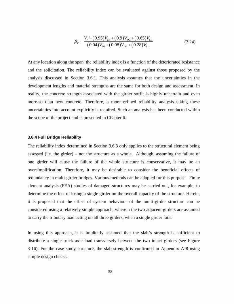
58
1 2
1 2
' 0.95 0.9 0.65
0.04 0.08 0.28
r D D LL
V
D D LL
V V V V
V V V
(3.24)
At any location along the span, the reliability index is a function of the deteriorated resistance
and the solicitation. The reliability index can be evaluated against those proposed by the
analysis discussed in Section 3.6.1. This analysis assumes that the uncertainties in the
development lengths and material strengths are the same for both design and assessment. In
reality, the concrete strength associated with the girder soffit is highly uncertain and even
more-so than new concrete. Therefore, a more refined reliability analysis taking these
uncertainties into account explicitly is required. Such an analysis has been conducted within
the scope of the project and is presented in Chapter 6.
3.6.4 Full Bridge Reliability
The reliability index determined in Section 3.6.3 only applies to the structural element being
assessed (i.e. the girder) – not the structure as a whole. Although, assuming the failure of
one girder will cause the failure of the whole structure is conservative, it may be an
oversimplification. Therefore, it may be desirable to consider the beneficial effects of
redundancy in multi-girder bridges. Various methods can be adopted for this purpose. Finite
element analysis (FEA) studies of damaged structures may be carried out, for example, to
determine the effect of losing a single girder on the overall capacity of the structure. Herein,
it is proposed that the effect of system behaviour of the multi-girder structure can be
considered using a relatively simple approach, wherein the two adjacent girders are assumed
to carry the tributary load acting on all three girders, when a single girder fails.
In using this approach, it is implicitly assumed that the slab‘s strength is sufficient to
distribute a single truck axle load transversely between the two intact girders (see Figure
3-16). For the case study structure, the slab strength is confirmed in Appendix A-8 using
simple design checks.
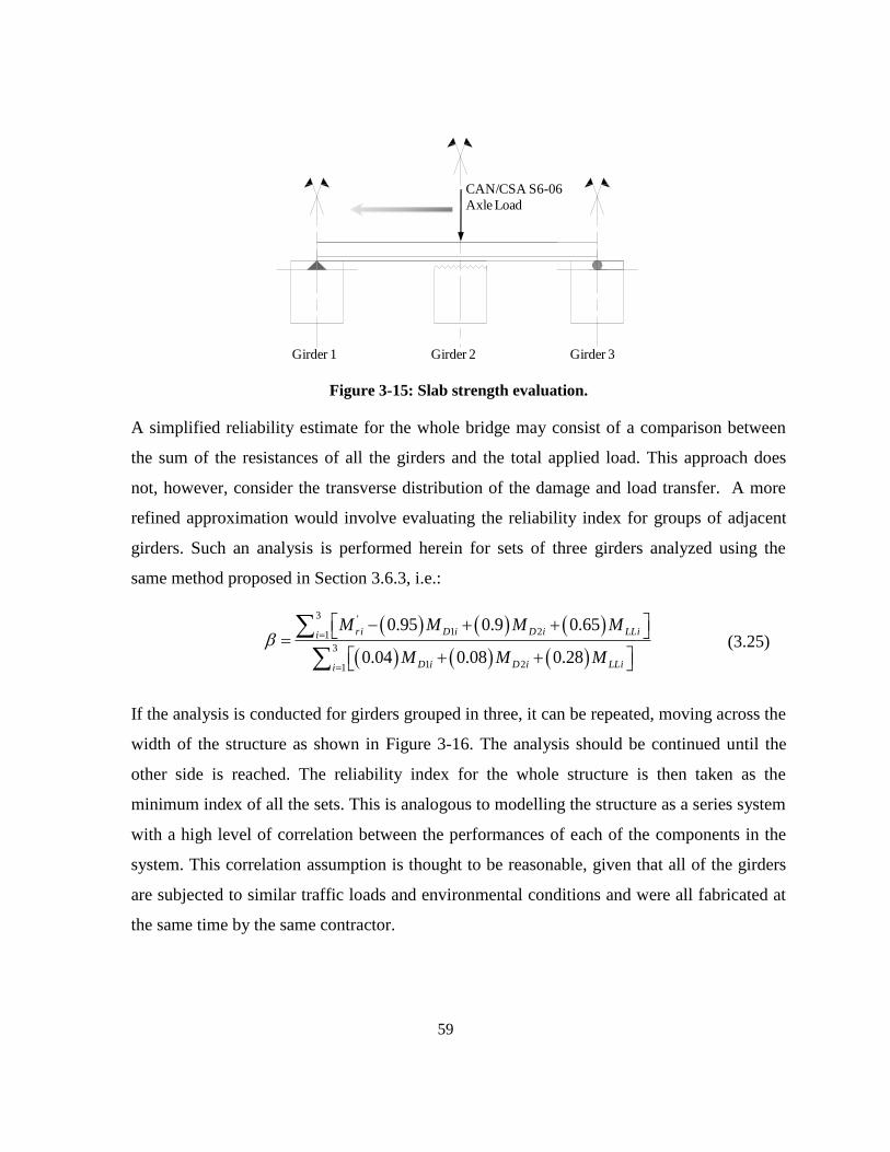
59
Figure 3-15: Slab strength evaluation.
A simplified reliability estimate for the whole bridge may consist of a comparison between
the sum of the resistances of all the girders and the total applied load. This approach does
not, however, consider the transverse distribution of the damage and load transfer. A more
refined approximation would involve evaluating the reliability index for groups of adjacent
girders. Such an analysis is performed herein for sets of three girders analyzed using the
same method proposed in Section 3.6.3, i.e.:
3 '
1 21
3
1 21
0.95 0.9 0.65
0.04 0.08 0.28
ri D i D i LLii
D i D i LLii
M M M M
M M M
(3.25)
If the analysis is conducted for girders grouped in three, it can be repeated, moving across the
width of the structure as shown in Figure 3-16. The analysis should be continued until the
other side is reached. The reliability index for the whole structure is then taken as the
minimum index of all the sets. This is analogous to modelling the structure as a series system
with a high level of correlation between the performances of each of the components in the
system. This correlation assumption is thought to be reasonable, given that all of the girders
are subjected to similar traffic loads and environmental conditions and were all fabricated at
the same time by the same contractor.
Girder 2Girder 1 Girder 3
CAN/CSA S6-06
Axle Load
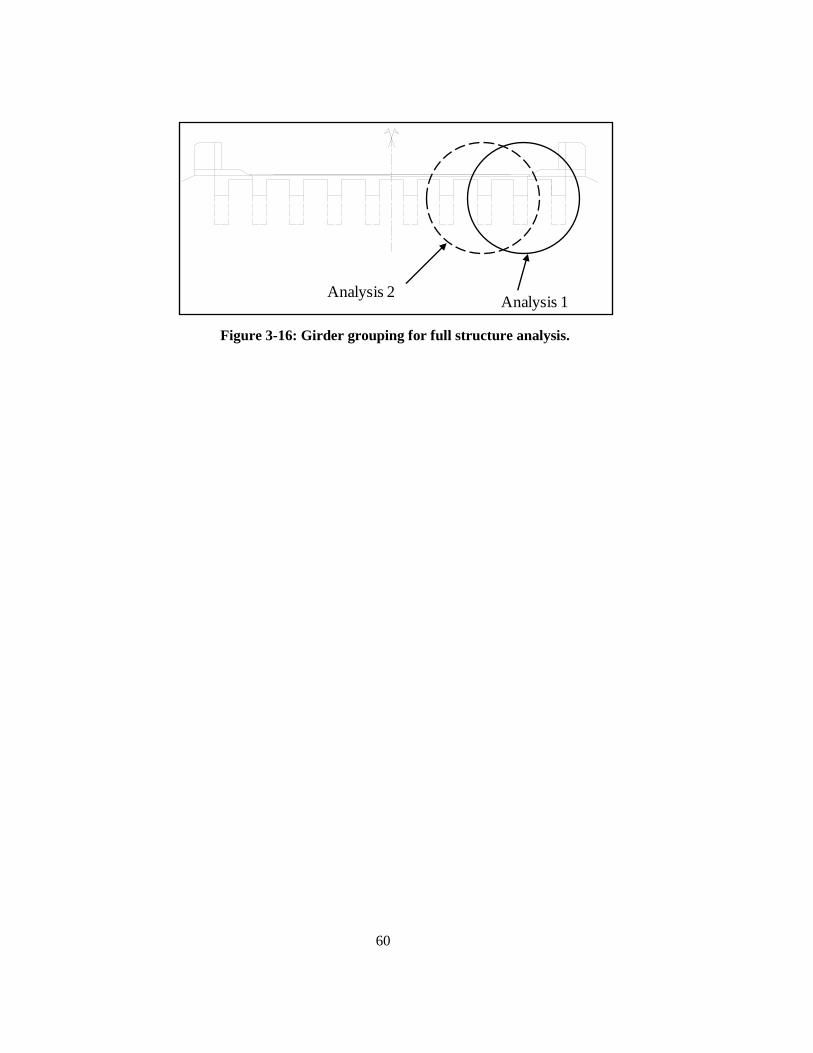
60
Figure 3-16: Girder grouping for full structure analysis.
Analysis 1Analysis 2

61
Chapter 4
Deterministic Analysis and Results
4.1 Introduction
The concept presented in Chapter 3 is best applied at multiple locations along the length of a
girder to evaluate the member‘s residual capacity. Both load effects, and resistance, clearly
vary along the length of a member. Geometric variations such as girder arching may also
vary significantly contributing to the flexural and shear capacities along the length of a
girder. In addition, a full scale structure generally requires reinforcement splices along its
length. An accurate model, such as that proposed in Chapter 3, considers strength variations
that occur as bars terminate with butt or staggered lap splices. A program is developed in
Matlab (2010) to conduct a multi-point analysis that considers strength and deterioration
variations to assess the capacity incrementally along each girder and ultimately the entire
bridge structure. In Section 4.2 the program was applied to a single girder to evaluate its
moment and shear capacities and reliability index. Next, Section 4.3 expands the program
for a multi-girder or full-bridge analysis. The program is then used to perform two short
sensitivity studies (Section 4.4). Finally, the code is expanded to consider section loss and
bond deterioration. The complete full bridge analysis program developed in this chapter has
been named BEST (Bridge Evaluation Strength Tool).
4.2 Single Girder Matlab Program
The modified area concept can easily be adapted to computer programming. The program
developed herein allows the user to evaluate the resistance of a single girder at a specified
number of points along its length. The program was developed in three steps corresponding
with: modified area, moment resistance and shear resistance computation.
4.2.1 Modified Area
To calculate the modified area, as discussed in Section 3.3.2, the algorithm described in
Figure 4-1 was followed.
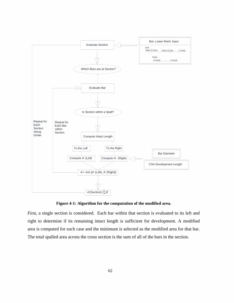
62
Figure 4-1: Algorithm for the computation of the modified area.
First, a single section is considered. Each bar within that section is evaluated to its left and
right to determine if its remaining intact length is sufficient for development. A modified
area is computed for each case and the minimum is selected as the modified area for that bar.
The total spalled area across the cross section is the sum of all of the bars in the section.
Start X-Cord.
Line
End X-Cord.
Point
Bot. Lower Reinf. Input
CSA Development Length
Bar Diameter
Y Cord.
X-Cord. Y-Cord.
Which Bars are at Section?
Evaluate Section
Is Section within a Spall?
Compute Intact Length
Compute A' (Left) Compute A' (Right)
Evaluate Bar
To the Left To the Right
Repeat for
Each Bar
within
Section
A'= min {A' (Left), A' (Right)}
A'(Section)= ? A'
Repeat for
Each
Section
Along
Girder
∑
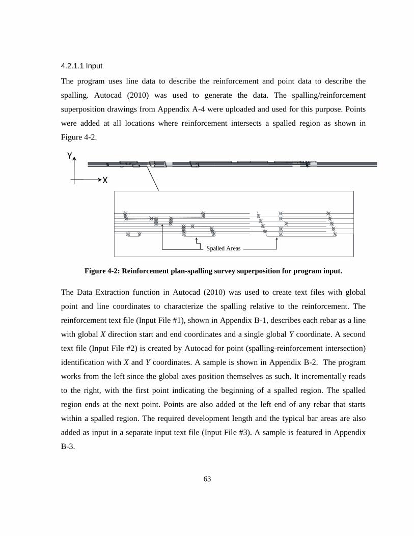
63
4.2.1.1 Input
The program uses line data to describe the reinforcement and point data to describe the
spalling. Autocad (2010) was used to generate the data. The spalling/reinforcement
superposition drawings from Appendix A-4 were uploaded and used for this purpose. Points
were added at all locations where reinforcement intersects a spalled region as shown in
Figure 4-2.
Figure 4-2: Reinforcement plan-spalling survey superposition for program input.
The Data Extraction function in Autocad (2010) was used to create text files with global
point and line coordinates to characterize the spalling relative to the reinforcement. The
reinforcement text file (Input File #1), shown in Appendix B-1, describes each rebar as a line
with global X direction start and end coordinates and a single global Y coordinate. A second
text file (Input File #2) is created by Autocad for point (spalling-reinforcement intersection)
identification with X and Y coordinates. A sample is shown in Appendix B-2. The program
works from the left since the global axes position themselves as such. It incrementally reads
to the right, with the first point indicating the beginning of a spalled region. The spalled
region ends at the next point. Points are also added at the left end of any rebar that starts
within a spalled region. The required development length and the typical bar areas are also
added as input in a separate input text file (Input File #3). A sample is featured in Appendix
B-3.
X
Y
Spalled Areas

64
4.2.1.2 Target formation
The program reads the input data within the Matlab directory and begins to rearrange it.
Based on equivalent Y coordinates the program relates the spalling points with their
associated reinforcing bar. Appendix B-5 shows the target formation for one section within
the first segment of the program. This represents the useable form to which the data has been
re-arranged. The target formation for a number of sections was checked with hand
calculations at an early stage in the program development. From this arrangement, the
minimum areas are next selected for each bar and the total modified and unmodified
reinforcement areas computed for the section.
4.2.2 Moment Resistance
The program uses the modified areas to compute a modified moment resistance using the
procedure described in Figure 4-3.
Figure 4-3: Algorithm for the computation of flexural capacity using the modified area concept.
Slab Self Weight Envelope
Girder Self Weight Envelope
Trans. Dist. FactorsLive Load Factor
Code Truck Envelope
Dynamic Load Allowance
Resistance Input
Material Properties
A'
CSA Moment CapacityResistance Factors
Sectional Properties
f'c fy Es
øc øs
Geometry Bot. Upper Reinf.
Unspalled MrSpalled Mr'
A
Plot
Solicitation Input
Dead Load Live Load
Dead Load Factor
65
Both spalled and unspalled moment resistance are found using the modified and unmodified
bar areas. Moment capacities were determined using CAN/CSA A23.3-04 rectangular stress
block theory. Bottom upper reinforcement was added (with no spalling effects considered)
while top upper reinforcement was conservatively ignored. In its current state, the program is
capable of analyzing T-beam as well as rectangular girder sections for flexure.
4.2.2.1 Program Input for Modified Moment Capacity
Input fields were separated into resistance (Input File #3) and solicitation (Input File #4) data
files. Sample input files can be found in Appendix B-3 and Appendix B-4 respectively.
Solicitation input consists of text files generated using the SAP program discussed in Section
3.2.4.1, copied to Input File #4. The dead loads, self weight of the slab and girder, and the
live load truck envelopes are kept separate in the input and are simply combined
arithmetically within the body of the program with the user specified transverse distribution
factor, dynamic load allowance (DLA), and load factors.
4.2.2.2 Program Output for Modified Moment Capacity
The program generates plots to graphically describe the deteriorated moment resistance.
Figure 4-4 shows the moment evaluation of Girder 2 in the case study structure (all girders
are of the same design). In the figure, the origin corresponds with the north girder support.
The south girder support corresponds to an X-coordinate of 1357 inches. In this analysis, the
girder was divided into 300 sections along its length, represented by points on the X-axis of
the plot.
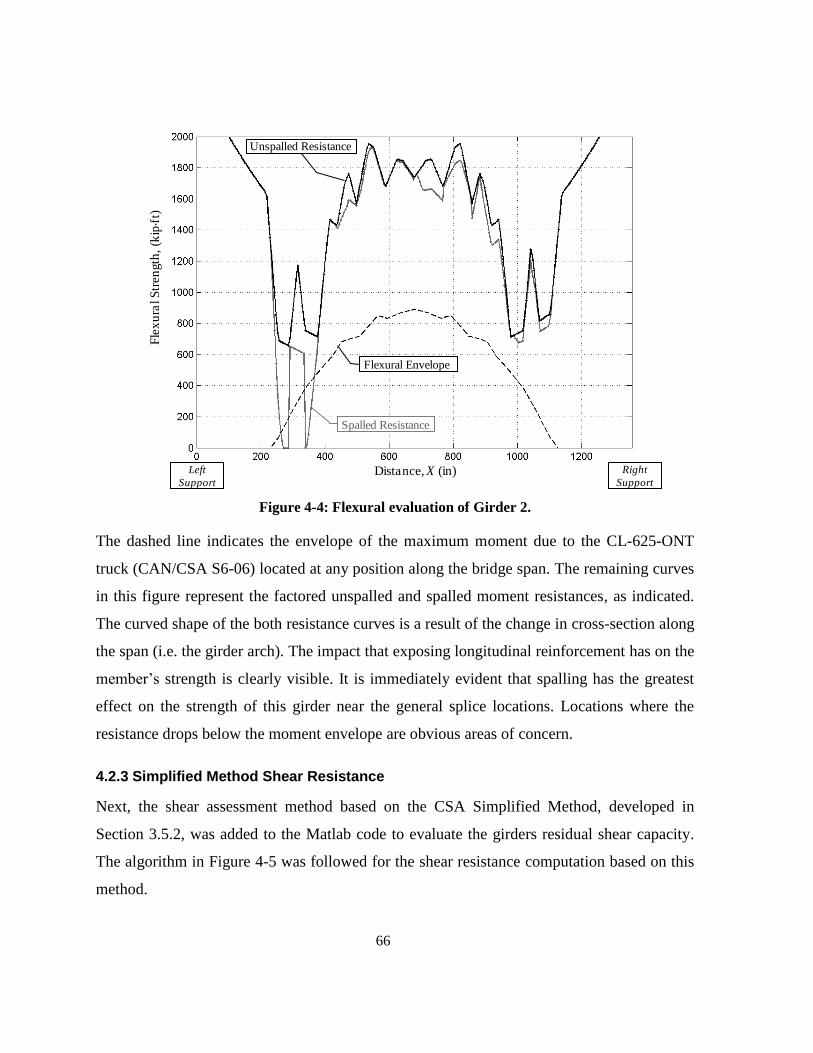
66
Figure 4-4: Flexural evaluation of Girder 2.
The dashed line indicates the envelope of the maximum moment due to the CL-625-ONT
truck (CAN/CSA S6-06) located at any position along the bridge span. The remaining curves
in this figure represent the factored unspalled and spalled moment resistances, as indicated.
The curved shape of the both resistance curves is a result of the change in cross-section along
the span (i.e. the girder arch). The impact that exposing longitudinal reinforcement has on the
member‘s strength is clearly visible. It is immediately evident that spalling has the greatest
effect on the strength of this girder near the general splice locations. Locations where the
resistance drops below the moment envelope are obvious areas of concern.
4.2.3 Simplified Method Shear Resistance
Next, the shear assessment method based on the CSA Simplified Method, developed in
Section 3.5.2, was added to the Matlab code to evaluate the girders residual shear capacity.
The algorithm in Figure 4-5 was followed for the shear resistance computation based on this
method.
Distance, X (in)
Spalled Resistance
Flexural Envelope
Unspalled Resistance
Left
Support
Right
Support
Fle
xu
ral S
tren
gth
, (k
ip∙f
t)

67
Figure 4-5: Algorithm for the computation of the shear capacity using the Simplified Shear
Method.
4.2.3.1 Program Input for Simplified Shear Method
An input field was added to Input File #3 to allow the user to specify the stirrup spacing and
any changes in this spacing along the length of the girder (Appendix B-3). For the case study
structure, minimum stirrups (as per CAN/CSA A23.3-04) were only provided within the 12
inch stirrup spacing sections to a distance of 252‖ (6400 mm) from the face of each support.
At the time of construction it is likely that provisions for minimum stirrups were not as
Material Properties
Stirrup Properties
Sectional Properties
f'c fy
Av Spacing
bw
Av (min) Provided?
Yes No
Sze=300mmSze per [1]Cl.11.3.6.3
Eqn(11-10)
A', Aex' per eqn 3.1
ß=0.18ß as per [1]Cl. 11.3.6.3 (b)(c)
Compute:
ß' (Eqn. 3.16)
?' (Eqn. 3.17)
Vr'(Eqn. 3.9-3.11)
Spalled CaseUnspalled Case
?=35°
Compute:
Vr (Eqn. 3.9-3.11)
Plot
ex per Cl.11.3.6.4
Eqn(11-11)
ββ
β'
εx
εx
θ'
θ
Vr’
fc' fy
Vr’
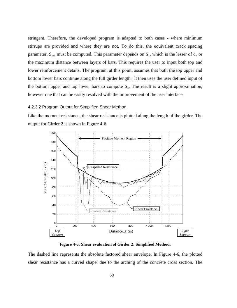
68
stringent. Therefore, the developed program is adapted to both cases - where minimum
stirrups are provided and where they are not. To do this, the equivalent crack spacing
parameter, Sze, must be computed. This parameter depends on Sz, which is the lesser of dv or
the maximum distance between layers of bars. This requires the user to input both top and
lower reinforcement details. The program, at this point, assumes that both the top upper and
bottom lower bars continue along the full girder length. It then uses the user defined input of
the bottom upper and top lower bars to compute Sz. The result is a slight approximation,
however one that can be easily resolved with the improvement of the user interface.
4.2.3.2 Program Output for Simplified Shear Method
Like the moment resistance, the shear resistance is plotted along the length of the girder. The
output for Girder 2 is shown in Figure 4-6.
Figure 4-6: Shear evaluation of Girder 2: Simplified Method.
The dashed line represents the absolute factored shear envelope. In Figure 4-6, the plotted
shear resistance has a curved shape, due to the arching of the concrete cross section. The
Distance, X (in)
Spalled ResistanceShear Envelope
Unspalled Resistance
Left
Support
Right
Support
Sh
ea
r S
tren
gth
, (k
ip)
Positive Moment Region

69
sudden jumps at 252‖ (6.4 m) and 1116‖ (28.35 m) from the left support represent changes in
the stirrup spacing. Since the observed spalling is contained to the girder soffit, the shear
resistance is only modified in the positive flexural zone (indicated on the plot), where the
bottom reinforcement is in tension.
4.2.4 Shear Resistance General Method
The shear resistance General Method discussed in Section 3.5.3 was also added to the Matlab
code. The algorithm in Figure 4-7 was followed for this method.
Figure 4-7: Algorithm for the computation of the shear capacity using the General Shear
Method.
Av (min) Provided?
Yes No
Sze=300mmSze per [1]Cl.11.3.6.3
Eqn(11-10)
A'
Spalled CaseUnspalled Case
Plot
ex' per eqn. 3.18ex per eqn. 3.18A
Compute:
ß' (Eqn. 3.16)
?' (Eqn. 3.17)
Vr'(Eqn. 3.9-3.11)
Compute:
ß (Eqn. 3.16)
? (Eqn. 3.17)
Vr(Eqn. 3.9-3.11)
Load Solicitation Input
Solicitation Input
Moment Envelope
Shear Envelope
β'
ε'xεx
θ'Vr’
β
θVr

70
4.2.4.1 Program Input for General Shear Method
The proposed General Method employs envelopes of the solicitation data. The moment and
shear envelopes are pre-determined within the code. The only adaption required is to adjust
the data series to be coincident with the points being analyzed along the girder. Linear
interpolation was used to approximate the moment and shear envelopes at each analysis
point.
4.2.4.2 Program Output for General Shear Method
The shear analysis output is shown graphically in Figure 4-8, again, for Girder 2.
Figure 4-8: Shear evaluation of Girder 2: General Method.
In the computation of the strain at mid-height, εx, the modified longitudinal bar area is used
and is subsequently responsible for the changes in the shape of the resistance plot. Sections
where the shear resistance drops below the shear envelope are areas of particular concern
from a structural safety standpoint.
Distance, X (in)
Spalled ResistanceShear Envelope
Left
Support
Right
Support
Sh
ea
r S
tren
gth
, (k
ip)
Unspalled Resistance
Positive Moment Region
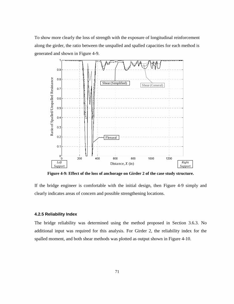
71
To show more clearly the loss of strength with the exposure of longitudinal reinforcement
along the girder, the ratio between the unspalled and spalled capacities for each method is
generated and shown in Figure 4-9.
Figure 4-9: Effect of the loss of anchorage on Girder 2 of the case study structure.
If the bridge engineer is comfortable with the initial design, then Figure 4-9 simply and
clearly indicates areas of concern and possible strengthening locations.
4.2.5 Reliability Index
The bridge reliability was determined using the method proposed in Section 3.6.3. No
additional input was required for this analysis. For Girder 2, the reliability index for the
spalled moment, and both shear methods was plotted as output shown in Figure 4-10.
Distance, X (in)
Shear (General)
Flexural
Shear (Simplified)
Left
Support
Right
Support
Ra
tio
of
Sp
alled
/Un
spa
lled
Resi
sta
nce
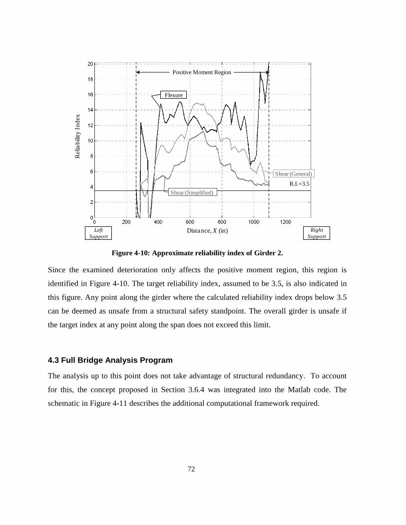
72
Figure 4-10: Approximate reliability index of Girder 2.
Since the examined deterioration only affects the positive moment region, this region is
identified in Figure 4-10. The target reliability index, assumed to be 3.5, is also indicated in
this figure. Any point along the girder where the calculated reliability index drops below 3.5
can be deemed as unsafe from a structural safety standpoint. The overall girder is unsafe if
the target index at any point along the span does not exceed this limit.
4.3 Full Bridge Analysis Program
The analysis up to this point does not take advantage of structural redundancy. To account
for this, the concept proposed in Section 3.6.4 was integrated into the Matlab code. The
schematic in Figure 4-11 describes the additional computational framework required.
Distance, X (in)
Shear (Simplified)
Left
Support
Right
Support
Relia
bilit
y I
nd
ex
Flexure
Positive Moment Region
Shear (General)
R.I.=3.5

73
Figure 4-11: Algorithm and file organization for multi-girder analysis.
4.3.1.1 Full Bridge Analysis Input
For a multi-girder or full structure analysis, managing the input data is a complex task. The
resistance and load input data remains the same as that for the single girder analysis but the
deterioration data (point and line coordinate text files) must be compiled for every girder. To
simplify the input, the point and line data for each girder was compiled into single text files
named based on the girder number and placed within a Matlab directory. A sample input file
can be found in Appendix B-6. As Matlab evaluates each girder, in order from Girder 1 to
Girder n, it scans the directory for the associated text file, reads it, and completes the
analysis.
Input File 5 for girders 1-nRead Input
'n'.txt
Create:
Multi Girder Analysis Results
Single Girder Analysis
Create:
Girder 'n'
Repeat for
Girder 1-n
Save: All plots for n
Full Bridge Analysis
Create:
Full Bridge Analysis
Save: All plots
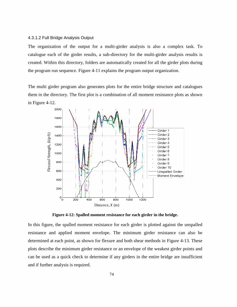
74
4.3.1.2 Full Bridge Analysis Output
The organization of the output for a multi-girder analysis is also a complex task. To
catalogue each of the girder results, a sub-directory for the multi-girder analysis results is
created. Within this directory, folders are automatically created for all the girder plots during
the program run sequence. Figure 4-11 explains the program output organization.
The multi girder program also generates plots for the entire bridge structure and catalogues
them in the directory. The first plot is a combination of all moment resistance plots as shown
in Figure 4-12.
Figure 4-12: Spalled moment resistance for each girder in the bridge.
In this figure, the spalled moment resistance for each girder is plotted against the unspalled
resistance and applied moment envelope. The minimum girder resistance can also be
determined at each point, as shown for flexure and both shear methods in Figure 4-13. These
plots describe the minimum girder resistance or an envelope of the weakest girder points and
can be used as a quick check to determine if any girders in the entire bridge are insufficient
and if further analysis is required.
Distance, X (in)
Fle
xu
ral S
tren
gth
, (k
ip∙f
t)

75
Distance, X (in)
Min. Spalled ResistanceShear Envelope
Left
Support
Right
Support
Sh
ea
r S
tren
gth
, (k
ip)
Unspalled Resistance
Positive Moment Region
Distance, X (in)
Min. Spalled ResistanceShear Envelope
Unspalled Resistance
Left
Support
Right
Support
Sh
ea
r S
tren
gth
, (k
ip)
Positive Moment Region
(a)
(b) (c)
Figure 4-13: Minimum spalled girder resistance for (a) Flexure, (b) Simplified Shear and (c)
General Shear Methods.
To consider structural redundancy, the method of girder groups proposed in Section 3.6.4 is
applied. In Figure 4-14 the results of the full bridge analysis are plotted for the flexural,
Simplified shear Method, and General shear Method verifications. Each curve represents the
minimum factored resistance ratio (resistance ÷ load effect) at each point along the span of
all groups of three (adjacent) girders analyzed. Although these curves still drop below 1.0 at
Distance, X (in)
Min. Spalled Resistance
Flexural Envelope
Unspalled Resistance
Left
Support
Right
Support
Fle
xu
ral S
tren
gth
, (k
ip∙f
t)

76
some locations along the span (indicating that the structure fails the verification at these
locations), the benefits of considering system behaviour are apparent.
Figure 4-14: Full bridge case study structure analysis using girder grouping presented as
resistance ratio.
Next the approximate reliability analysis concept presented in Section 3.6.4 was employed,
and the reliability index for each set of three girders transversely across the structure was
determined. Finally, the minimum reliability index for any group of three girders is found at
each point and plotted as the full bridge reliability output as shown in Figure 4-15. The
absolute minimum is taken as the reliability index for the whole structure.
Distance, X (in)
Shear (Simplified)
Left
Support
Right
Support
Resi
sta
nce
Ra
tio
Flexure
Positive Moment Region
Shear (General)
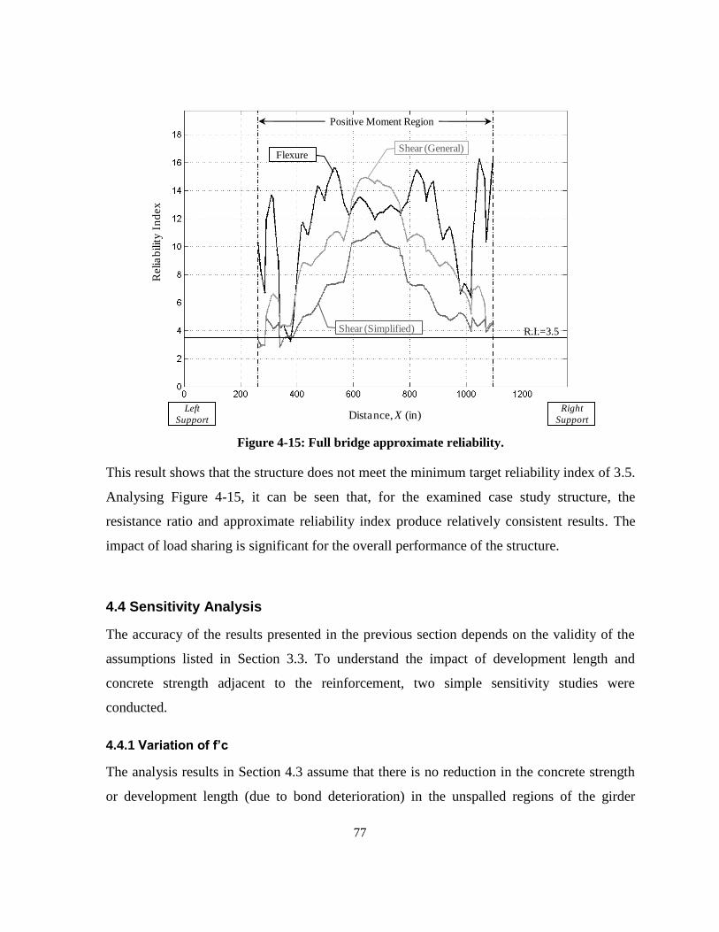
77
Figure 4-15: Full bridge approximate reliability.
This result shows that the structure does not meet the minimum target reliability index of 3.5.
Analysing Figure 4-15, it can be seen that, for the examined case study structure, the
resistance ratio and approximate reliability index produce relatively consistent results. The
impact of load sharing is significant for the overall performance of the structure.
4.4 Sensitivity Analysis
The accuracy of the results presented in the previous section depends on the validity of the
assumptions listed in Section 3.3. To understand the impact of development length and
concrete strength adjacent to the reinforcement, two simple sensitivity studies were
conducted.
4.4.1 Variation of f’c
The analysis results in Section 4.3 assume that there is no reduction in the concrete strength
or development length (due to bond deterioration) in the unspalled regions of the girder
Distance, X (in)
Shear (Simplified)
Left
Support
Right
Support
Relia
bilit
y I
nd
ex
Flexure
Positive Moment Region
Shear (General)
R.I.=3.5
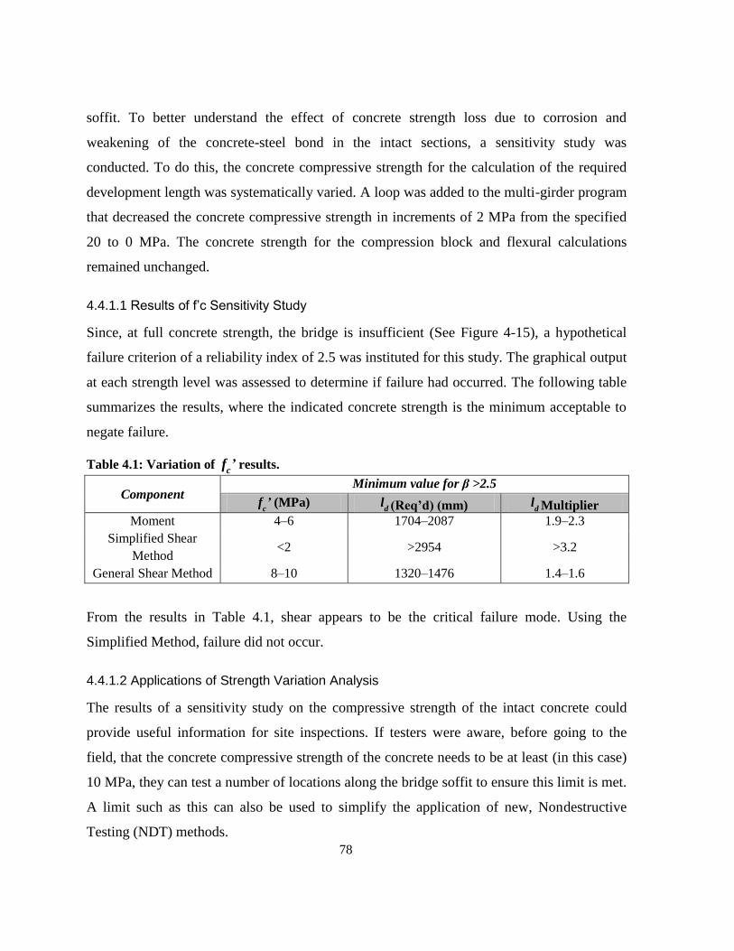
78
soffit. To better understand the effect of concrete strength loss due to corrosion and
weakening of the concrete-steel bond in the intact sections, a sensitivity study was
conducted. To do this, the concrete compressive strength for the calculation of the required
development length was systematically varied. A loop was added to the multi-girder program
that decreased the concrete compressive strength in increments of 2 MPa from the specified
20 to 0 MPa. The concrete strength for the compression block and flexural calculations
remained unchanged.
4.4.1.1 Results of f’c Sensitivity Study
Since, at full concrete strength, the bridge is insufficient (See Figure 4-15), a hypothetical
failure criterion of a reliability index of 2.5 was instituted for this study. The graphical output
at each strength level was assessed to determine if failure had occurred. The following table
summarizes the results, where the indicated concrete strength is the minimum acceptable to
negate failure.
Table 4.1: Variation of fc’ results.
Component Minimum value for β >2.5
fc’ (MPa) l
d (Req’d) (mm) ld Multiplier
Moment 4–6 1704–2087 1.9–2.3
Simplified Shear
Method <2 >2954 >3.2
General Shear Method 8–10 1320–1476 1.4–1.6
From the results in Table 4.1, shear appears to be the critical failure mode. Using the
Simplified Method, failure did not occur.
4.4.1.2 Applications of Strength Variation Analysis
The results of a sensitivity study on the compressive strength of the intact concrete could
provide useful information for site inspections. If testers were aware, before going to the
field, that the concrete compressive strength of the concrete needs to be at least (in this case)
10 MPa, they can test a number of locations along the bridge soffit to ensure this limit is met.
A limit such as this can also be used to simplify the application of new, Nondestructive
Testing (NDT) methods.

79
4.4.2 Future Deterioration Estimate
To showcase how the BEST computer program could be used to forecast bridge
performance, the spalled regions were systematically scaled up to model future deterioration.
It is understood that as time progresses, new spalled regions develops and existing ones
increase in size as the nearby concrete (and steel) deteriorates. The following figure shows
the scaling of spalled regions by area as assumed in the analysis.
Figure 4-16: Spalling scale-up analysis.
The results of this study are shown in Appendix B-7. Although the results are as predicted,
i.e. a decrease in capacity as the spalled area increases, the following should be noted from
the study: It is not sufficient to simply model the effect of spalling over time by increasing
the required development length. As the spalled regions increase in size, they may begin to
affect adjacent bars that previously were fully developed. Therefore the effect of spalling
over time is difficult to quantify and would greatly benefit from addition research to study
the development of spalling with time.
4.5 Corrosion Section Loss Model
In the presented formulation, up to this point, it has been assumed that the steel rebar itself is
not significantly deteriorated. Using the methodology described in Chapter 2, a reduction in
the rebar yield strength, i.e. based on Equation 4.1, can be introduced. To demonstrate this,
Girder #9
x 1.25
x 1.5
x 2

80
the empirical model by Cairns et al. (2005) and Lee and Cho (2009) with αy = 0.012 was
selected for the current study. The selected model is identified in Figure 4-17. Other
empirical models could be used in place of the adopted model. However, this model was
chosen as it gives average predictions compared with the other models in Figure 4-17 and
was validated using a relatively large database of test results.
Figure 4-17: Selected empirical model for residual yield strength of corroded bars.
The following relationship was thus added to the multi-girder program:
(1.0 0.012 )y corr yof Q f (4.1)
The program does not further modify the bar‘s cross-sectional areas, but rather modifies the
bar‘s yield strength according to Equation 4.1.
4.5.1 Corrosion Model Input
A new field was added to the input file to allow the user to enter an average percent corrosion
for both intact concrete sections, Qi, and sections of steel within spalled regions, Qs. The
exposure of steel within spalled regions is greater when the protective concrete cover is no
0
0.2
0.4
0.6
0.8
1
0 10 20 30
Modif
ied Y
ield
Str
ength
(f y
/fyo)
Average Section Loss (% of Original)
Morinaga 1996
Zhang et al. 1995
Cairns et al. 2005, Lee et al. 1996
Du 2001, Andrade et al. 1991
Clark and Saifullah 1994

81
longer in place. The corrosion levels, at this time, are unknown for the case study structure
and therefore the degree of corrosion was left as a user input. For application to actual
structures, this parameter could be measured or estimated.
4.5.2 Corrosion Model Output
For demonstration purposes, 15% corrosion within spalled regions and 6% corrosion in intact
concrete was used. The full output for this case is provided in Appendix B-8 for Girder 2. For
the full bridge analysis, the resistance ratio and reliability index shifted to that shown in
Figure 4-18 and Figure 4-19.
Figure 4-18: Full bridge resistance ratio with section loss model.
Distance, X (in)
Shear (Simplified)
Left
Support
Right
Support
Dete
rio
rate
d R
esi
sta
nce
Ra
tio
(R
r/R
f)
Flexure
Positive Moment Region
Shear (General)

82
Figure 4-19: Full bridge reliability with section loss model.
The results show, as expected, a shift downward in the calculated resistance ratio and
reliability index due to spalling and structural deterioration.
4.6 Bond Deterioration Model
In the analysis procedures described in Chapter 2, it has been assumed that the intact concrete
adjacent to the spalled regions can continue to provide the same bond as it did in the new
structure. However, if spalling has occurred, there is sufficient evidence that reinforcing
corrosion has also taken place and the bond strength between reinforcing steel and concrete
has deteriorated. For the purpose of this study, the empirical model proposed by Bhargava et
al. (2007) (see Figure 4-20) was selected based on the range of test data and consideration
given in this reference of previous studies.
Right
SupportDistance, X (in)
Shear (Simplified)
Left
Support
Relia
bilit
y I
nd
ex
Flexure
Positive Moment Region
Shear (General)
R.I.=3.5

83
Figure 4-20: Selected empirical relationship for steel deterioration.
The model assumes that longitudinal cracking occurs at 1.5% corrosion (Xp = 1.5%) and:
1.0 for 1.5%pR X (4.2)
0.198
1.34 for 1.5%pX
pR e X
where,
Xp = average section loss as a percentage of the original cross section area
R = ratio of the current to the original bond strength
For this model, the average corrosion, Xp, is equivalent to Qi, or the average corrosion level
within the intact sections.
0
0.2
0.4
0.6
0.8
1
0 5 10 15 20 25 30
R =
Det
erio
rate
d B
ond S
tren
gth
/In
itia
l B
on
d S
tren
gth
Degree of Corrosion (%)
Bhargava et al. 2005 (Pullout)Chung et al. 2004 Bhargava et al. 2007 (Beam)Lee et al. 2002Rodriguez et al. 1994 (upper bound)Stanish et al. 1999Rodriguez et al. 1994 (lower bound)CONTECVET 2001 Cabrera and Ghoddoussi 1992

84
This model was easily integrated into the multi-girder program. With the addition of this
model and the case of Qs=15% and Qi=6%, the results of the full bridge analysis are
presented in Figure 4-21 and Figure 4-20.
Figure 4-21: Full bridge resistance ratio with section loss and bond deterioration.
Distance, X (in)
Shear (Simplified)
Left
Support
Right
Support
Dete
rio
rate
d R
esi
sta
nce
Ra
tio
(R
r/R
f)
Flexure
Positive Moment Region
Shear (General)
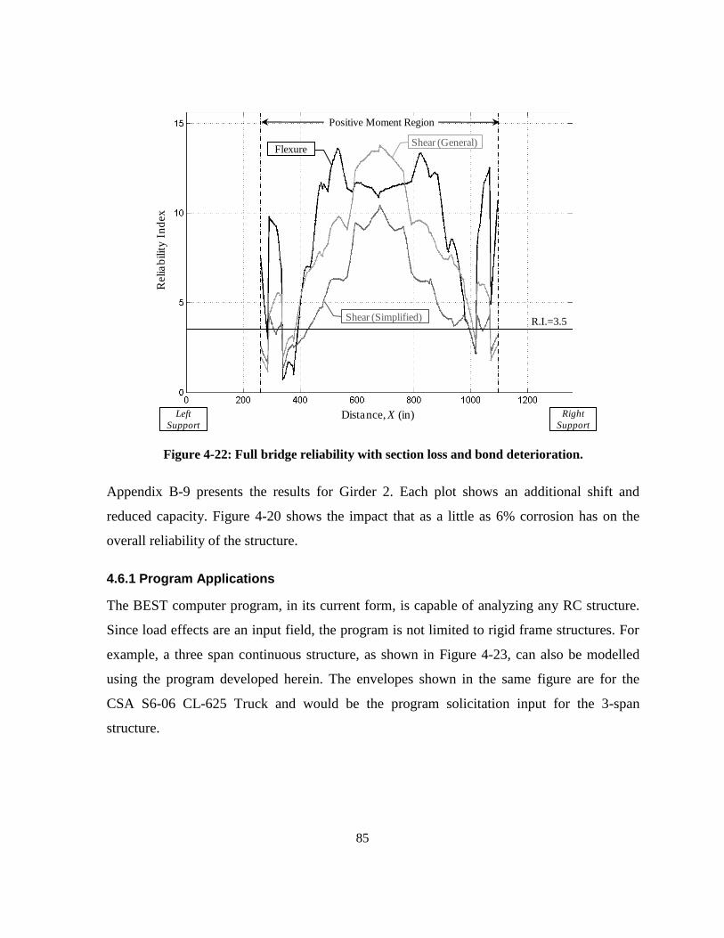
85
Figure 4-22: Full bridge reliability with section loss and bond deterioration.
Appendix B-9 presents the results for Girder 2. Each plot shows an additional shift and
reduced capacity. Figure 4-20 shows the impact that as a little as 6% corrosion has on the
overall reliability of the structure.
4.6.1 Program Applications
The BEST computer program, in its current form, is capable of analyzing any RC structure.
Since load effects are an input field, the program is not limited to rigid frame structures. For
example, a three span continuous structure, as shown in Figure 4-23, can also be modelled
using the program developed herein. The envelopes shown in the same figure are for the
CSA S6-06 CL-625 Truck and would be the program solicitation input for the 3-span
structure.
Right
SupportDistance, X (in)
Shear (Simplified)
Left
Support
Relia
bilit
y I
nd
ex
Flexure
Positive Moment Region
Shear (General)
R.I.=3.5

86
Figure 4-23: Moment and shear envelopes for a 3-span continuous girder.
In addition, because the load effects are input by the user, the user can control the accuracy
of the model and subsequently the program. As a quick check, or analysis, the user may
decide to use simple hand calculations to generate the load effects. For example, the analysis
of the case study structure used the finite element model discussed in Section 3.2.4.1. As a
simple, quick analysis, the bridge evaluator may decide to use an average cross section and
analyse the structure as fixed-fixed or simply supported. In this case, the user controls the
accuracy of the program and is cautioned to use ‗safe‘ judgment.
Although, the CSA transverse distribution model was used for this analysis, any transverse
distribution model that utilizes similar distribution factors may be used. Similarly, the
required development length was calculated using CSA provisions, but other code or
empirical relations may be used.
Mom
ent
Distance
Sh
ear
Distance

87
Since load and resistance factors are user specified, the user can easily perform both nominal
and factored analyses for the given structure. Nominal analysis, for example (with load and
resistance factors all set to equal 1.0), may be used to predict laboratory test results.
The section depth and stirrup spacing may also be varied along the length or the girder, as is
the case with the arched case study structure
4.6.2 Program Limitations
The program currently has a number of restrictions in place so that it could be simply created
and interpreted. The program, in its current form, only allows for two layers of bottom
reinforcement to be considered for flexural resistance. These bars, however, must have a
constant bar diameter. Future versions of the program can expand the input if these features
are found to limit users. The geometry is also limited to rectangular and T-shaped sections.
Since this covers the majority of conventionally reinforced bridges, adaption to other
geometries at this time may not be a priority.
Also, the program is currently limited to the CSA approach for calculating flexural and shear
resistance. Little work would be required, however, to create versions of the program for
other national standards.

88
Chapter 5
Experimental Program and Results
5.1 Introduction
A pilot laboratory study was conducted to do the following:
a) determine if the proposed modified area concept and BEST computer program can
predict the behaviour of a mechanically spalled concrete beam with exposed
reinforcement,
b) determine if planes of weakness are created between the spalled patches,
c) determine the effect, if any, of asymmetric spalling on a concrete beam‘s strength, e.g.
spalling occurring only on one half of a girder with the other half intact,
d) determine the effectiveness of a mortar patch (as currently utilized in industry) to
restoring bond and strength, and
e) explore FRP repairs for bond, flexural and shear strength restoration.
The current chapter describes this pilot study and presents the main results.
5.2 Test Program
Twelve test beams were fabricated in total. They are divided into reference, spalled and
deterioration specimens as indicated by the matrix shown in Table 5.1.
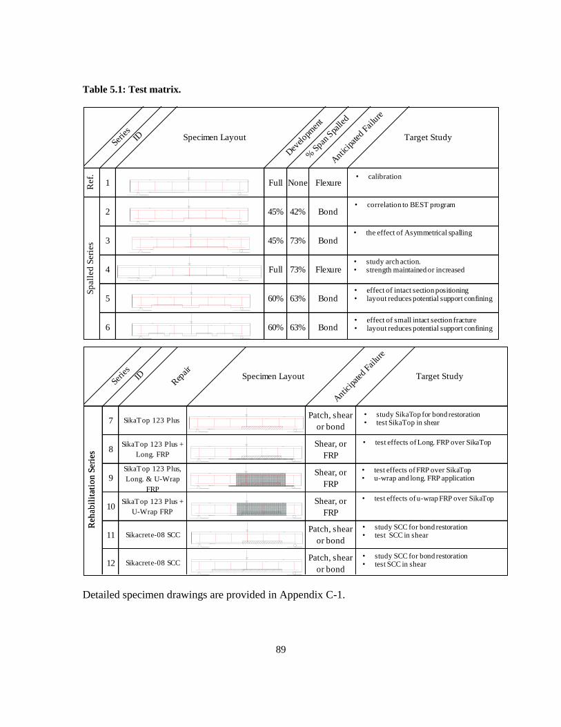
89
Table 5.1: Test matrix.
Detailed specimen drawings are provided in Appendix C-1.
Serie
sID Specimen Layout
Dev
elopm
ent
% S
pan S
palle
d
Antic
ipated
Fai
lure
Target Study
Ref.
1 Full None Flexure
2 45% 42% Bond
3 45% 73% Bond
4 Full 73% Flexure
5 60% 63% Bond
6 60% 63% Bond
Sp
all
ed
Seri
es
• calibration
• correlation to BEST program
• the effect of Asymmetrical spalling
• study arch action. • strength maintained or increased
• effect of intact section positioning• layout reduces potential support confining
• effect of small intact section fracture• layout reduces potential support confining
Serie
sID
Rep
air Specimen Layout
Antic
ipated
Fai
lure
Target Study
Reh
ab
ilit
ati
on
Seri
es
7 SikaTop 123 Plus Patch, shear
or bond
8SikaTop 123 Plus +
Long. FRP
Shear, or
FRP
9SikaTop 123 Plus,
Long. & U-Wrap
FRP
Shear, or
FRP
10SikaTop 123 Plus +
U-Wrap FRP
Shear, or
FRP
11 Sikacrete-08 SCCPatch, shear
or bond
12 Sikacrete-08 SCCPatch, shear
or bond
Reh
ab
ilit
ati
on
Seri
es
• test effects of u-wrap FRP over SikaTop
• study SikaTop for bond restoration• test SikaTop in shear
• test effects of Long. FRP over SikaTop
• test effects of FRP over SikaTop• u-wrap and long. FRP application
• study SCC for bond restoration• test SCC in shear
• study SCC for bond restoration• test SCC in shear

90
1200100
8-3/16" Stirrups @ 200mm
100
2-1/4" x 1400mm Smooth
Bars
2-10M x 1240mm
25
20
2- 10M Bars
2 - 1/4" Smooth Bars
1503
16" Stirrups
100
Beam #1
20
150
25
100
2 – 1/4" Smooth Bars
3/16‖ Stirrups
2 – 10M Bars
5.2.1 Test Specimens
A scaled-down rectangular cross section, as shown in Figure 4-13, was selected to reduce
material costs and utilize existing formwork.
Figure 5-1: Typical test specimen (a) Cross section and (b) Elevation.
The beams were designed for an underreinforced flexural failure. The design calculations are
provided in Appendix C-2.
5.2.2 Material Properties
Reinforcing Steel
10M 400 grade longitudinal reinforcing steel was used. Canadian steel was specified for
quality and consistency. The reinforcing bars were wired brush cleaned before the repairs
were applied.
(b)
(a)
1200100
8-3/16" Stirrups @ 200mm
100
2-1/4" x 1400mm Smooth
Bars
2-10M x 1240mm
25
20
2- 10M Bars
2 - 1/4" Smooth Bars
1503
16" Stirrups
100
Beam #1Beam #1
100
100 1200
2 – 1/4" × 1400mm Smooth Bars
8 – 3/16‖ Stirrups @ 200mm
2 – 10M 1240mm

91
Concrete
A concrete compressive strength of 20-25 MPa was specified to replicate the concrete
originally specified on the case study structure. 9 mm aggregate was specified in view of the
reduced scale of the tested beams. The concrete was cured under wet burlap and plastic to
keep it moist. Concrete cylinders were tested at 7, 14, 21, and 28 days. The 28 day
compressive strength was 16.1 MPa.
5.2.3 Deterioration
Artificial spalling was achieved using cast-in foam blocks. The blocks were chipped out at 7
days to create pockets to simulate spalling as shown in Figure 5-2.
Figure 5-2: Cast-in foam blocks for spalling simulation.
For the test specimens set to be repaired, the surface was roughened using a needle peener to
achieve the results shown in Figure 5-3.
Figure 5-3: Surface roughened by needle peener and strain gauge installation.
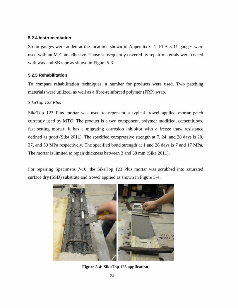
92
5.2.4 Instrumentation
Strain gauges were added at the locations shown in Appendix C-1. FLA-5-11 gauges were
used with an M-Cote adhesive. Those subsequently covered by repair materials were coated
with wax and SB tape as shown in Figure 5-3.
5.2.5 Rehabilitation
To compare rehabilitation techniques, a number for products were used. Two patching
materials were utilized, as well as a fibre-reinforced polymer (FRP) wrap.
SikaTop 123 Plus
SikaTop 123 Plus mortar was used to represent a typical trowel applied mortar patch
currently used by MTO. The product is a two component, polymer modified, cementitious,
fast setting mortar. It has a migrating corrosion inhibitor with a freeze thaw resistance
defined as good (Sika 2011). The specified compressive strength at 7, 24, and 28 days is 20,
37, and 50 MPa respectively. The specified bond strength at 1 and 28 days is 7 and 17 MPa.
The mortar is limited to repair thickness between 3 and 38 mm (Sika 2011).
For repairing Specimens 7-10, the SikaTop 123 Plus mortar was scrubbed into saturated
surface dry (SSD) substrate and trowel applied as shown in Figure 5-4.
Figure 5-4: SikaTop 123 application.
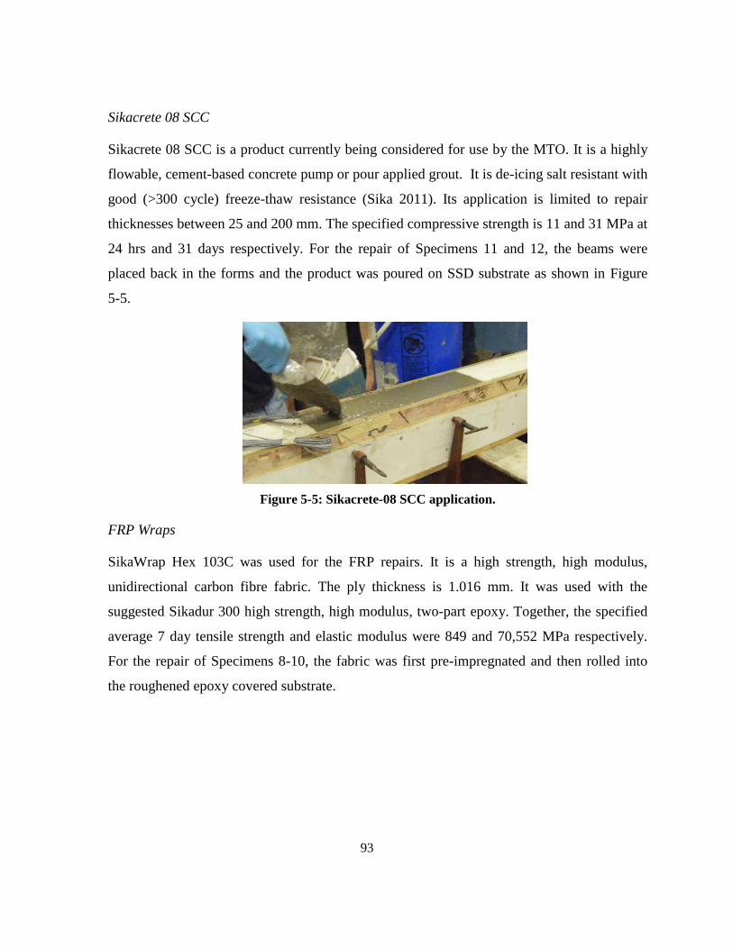
93
Sikacrete 08 SCC
Sikacrete 08 SCC is a product currently being considered for use by the MTO. It is a highly
flowable, cement-based concrete pump or pour applied grout. It is de-icing salt resistant with
good (>300 cycle) freeze-thaw resistance (Sika 2011). Its application is limited to repair
thicknesses between 25 and 200 mm. The specified compressive strength is 11 and 31 MPa at
24 hrs and 31 days respectively. For the repair of Specimens 11 and 12, the beams were
placed back in the forms and the product was poured on SSD substrate as shown in Figure
5-5.
Figure 5-5: Sikacrete-08 SCC application.
FRP Wraps
SikaWrap Hex 103C was used for the FRP repairs. It is a high strength, high modulus,
unidirectional carbon fibre fabric. The ply thickness is 1.016 mm. It was used with the
suggested Sikadur 300 high strength, high modulus, two-part epoxy. Together, the specified
average 7 day tensile strength and elastic modulus were 849 and 70,552 MPa respectively.
For the repair of Specimens 8-10, the fabric was first pre-impregnated and then rolled into
the roughened epoxy covered substrate.

94
5.3 Test Results and Discussion
In this section, the results for each reference, spalling and rehabilitation series are as follows.
Both ultimate and serviceability related performance metrics are discussed.
5.3.1 Reference Beam
Beam 1 was unspalled and serves as a reference for all other test specimens. As shown in
Appendix C-2, the beam was designed for shear failure. Even though minimum stirrups (as
per CAN/CSA A23.3-04) were provided, it is expected that the stirrups did not contribute to
the shear strength due to the mortar strength, stirrup spacing, use of round 9 mm aggregate
and the use of smooth wire stirrups. In fact, many older bridge structures are shear sensitive
and do not meet modern shear standards. For example, minimum stirrups were not provided
along the majority of the case study structure girder span.
Using the actual 28 day concrete compressive strength (16.1 MPa) and the specified steel
strength (400 MPa), the strength of the member is shown as case (a) in Table 5.2. To
understand the failure, case (b) was created with the average concrete strength at the day of
testing (18 MPa) and an anticipated actual steel strength of 450 MPa. These are more realistic
actual material strengths. Actual results indicate that, overall, the beam is shear sensitive.
Table 5.2: Strength approximations of Beam 1.
*Strengths shown in applied load (kN).
In fact, the beam is on the verge of flexure and shear failure and interestingly, the
conservatism of the each code strength approximation is well displayed. That is, potentially
the conservatism in the flexure strength is higher than that of the General shear Method.
Flexural
StrengthActual
Case Vc Vs Vr Vc Vs Vr MrFailure
Load
(a) 17.22 41.27 30.3 30.3 23.90
(b) 18.26 18.26 31.8 31.8 26.7426.40
Simplified Method General Method

95
Herein, the material strengths proposed in case (b) are used and it has been assumed that the
stirrups do not contribute to the shear strength of the member.
5.3.2 Spalling Series
The results of the spalling series tests are discussed in terms of member strength and
ductility.
Member Strength
The predicted strengths for each test specimen using the BEST program are shown in Table
5.3 (converted to applied load values). The resistances predicted by the proposed flexural and
shear methods are shown in this table. The selected lowest (critical) strengths are highlighted
and compared to actual test results. BEST selects the lowest of flexure and shear strengths for
the member. Test:predicted values range between 1.55-1.21. In each case, the estimate is
conservative. Based on this estimate, the failure mode should be characterized as a shear-
bond failure. In reality, however, the actual observed failure of each member (other than
Beam 4) was flexure-bond or ‗pure‘ anchorage failure. Therefore, it is anticipated that the
strengths governed by flexure are likely a more accurate representation. As shown in Table
5.3, test:predicted values range between 1.28-0.87 for this case.
Table 5.3: Strength approximation for spalling series beams.
*Strengths in applied load (kN).
Serie
s
Bea
m ID
Spall P
attern
Dev
elopm
ent
% S
pan S
palle
d
Failu
re L
oad (k
N)
Flexu
re
Simplif
ied M
ethod
Gen
eral M
ethod
Selec
ted
Flexu
re O
nly
Flexu
re or S
hear
Predicted Strength* Test/PredictedSpecimen Layout Actual*
2 45% 42% 17.16 13.40 11.10 20.30 11.10 1.28 1.55
3 45% 73% 16.64 13.40 11.10 20.30 11.10 1.24 1.50
4 Full 73% 24.20 26.70 18.26 27.15 18.26 0.91 1.33
5 60% 63% 17.36 18.20 13.20 23.14 13.20 0.95 1.32
6 60% 63% 15.91 18.20 13.20 23.14 13.20 0.87 1.21
Sp
all
ed
Seri
es
Predicted Strength* Test/PredictedSpecimen Layout
96
As anticipated, Beam 2, which had asymmetrical simulated spalling, failed in bond. The
crack pattern for the beam is shown in Table 5.4. The BEST program predicted strength
appears to be highly conservative. It is likely that this conservatism is due to additional
confining stress over the right support, which is not considered by BEST. The bond strength
in this section is increased due to the intersection of the inclined shear path with the
anchorage zone and bearing surface. Beam 3 has the same development length (180 mm), but
is spalled symmetrically over 73% of the span. Marginal differences in strength between
Beam 2 and Beam 3 indicate that the symmetric nature of spalling has little or no effect
because failure in both cases was due to bond.
In Beam 4, the longitudinal bars were fully anchored by extending them past the supports.
The results for this beam serve as a good example of a shift from shear failure to arch action.
Steel gauge strains indicate a shift upward of the neutral axis and a change in failure mode to
concrete crushing failure. The crack pattern, shown in Table 5.4, matches those observed by
Cairns and Zhao (1993). High deflections, exceeding one degree of rotation, are apparent. In
actual bridge structures, deflections of this magnitude are visible and likely detectable. For
the case of full development, BEST anticipates the strength to be equal to that of the
unspalled beam.
In Beam 5, 240 mm of development length is provided, to accommodate a spalling pattern in
which 90 mm is intact on each side of the centrally placed load. The results indicate that
BEST is less conservative (unconservative in flexure) for this case due to the apparent
inability of the central intact section to engage and contribute to anchorage. It is likely that a
section of this nature acts similarly to a pivot for the longitudinal reinforcing steel. The
vertical cracks near the central intact section (shown in Table 5.4) support this theory. A
simple approach may be to neglect intact section near the load point(s). In this case, if the
intact section is removed, the test:predicted ratio for flexure increases from 0.95 to 1.525.

97
Table 5.4: Test specimen crack patterns.
Beam 6 had similar short intact sections within the span. In this beam, the central section was
shortened to 60 mm on each side of the centrally placed load and additional small intact
sections (60 mm) were created further away on either side. The total development length
provided was the same as that for Beam 5 (230 mm). A further strength reduction is seen for
Beam 6, due in part to the fracture of one of the short intact sections before the final pullout
failure. The cracked section is shown in Figure 5-6. The fracture of intact sections depends
on the shear strength of the section, which is a function of the concrete strength, intact length
and depth of spalling. It also depends on the tensile force in the reinforcing bar at that
Serie
s
Bea
m ID
Cracked Specimen
Ref
.
1
2
3
4
5
6
7
8
9
10
11
12
Sp
alle
d S
erie
sR
ehab
ilitat
ion
Ser
ies
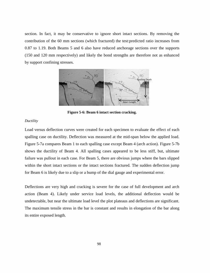
98
section. In fact, it may be conservative to ignore short intact sections. By removing the
contribution of the 60 mm sections (which fractured) the test:predicted ratio increases from
0.87 to 1.19. Both Beams 5 and 6 also have reduced anchorage sections over the supports
(150 and 120 mm respectively) and likely the bond strengths are therefore not as enhanced
by support confining stresses.
Figure 5-6: Beam 6 intact section cracking.
Ductility
Load versus deflection curves were created for each specimen to evaluate the effect of each
spalling case on ductility. Deflection was measured at the mid-span below the applied load.
Figure 5-7a compares Beam 1 to each spalling case except Beam 4 (arch action). Figure 5-7b
shows the ductility of Beam 4. All spalling cases appeared to be less stiff, but, ultimate
failure was pullout in each case. For Beam 5, there are obvious jumps where the bars slipped
within the short intact sections or the intact sections fractured. The sudden deflection jump
for Beam 6 is likely due to a slip or a bump of the dial gauge and experimental error.
Deflections are very high and cracking is severe for the case of full development and arch
action (Beam 4). Likely under service load levels, the additional deflection would be
undetectable, but near the ultimate load level the plot plateaus and deflections are significant.
The maximum tensile stress in the bar is constant and results in elongation of the bar along
its entire exposed length.
32°
Intact Length
Spalling Depth

99
0
5
10
15
20
25
30
0 2 4 6 8 10 12L
oad
(kN
)Mid-Span Deflection (mm)
Beam 1Beam 3Beam 4
Figure 5-7: Spalling Series load-deflection curves for (a) Spalling configurations and (b) Arch
action.
5.3.3 Rehabilitation Series
Member Strength
All repairs (except the ones applied to Beam 12) were applied to the same spalling case as
Beam 2. If the repair was sufficient, then the strength of the spalled (right) side of the beam
was sufficiently restored to force shear failure to the left (substrate) side of the beam. As
shown in Table 5.5, each repair was sufficient to restore the bond and subsequently the beam
strength. In Table 5.5 the strengths are compared to the unspalled beam as the
repaired:unspalled ratio. The variations in this ratio are likely governed by the experimental
variation of the shear strength of the substrate concrete. Both the mortar patch and SCC
repair were easy to trowel apply and appeared to bond well to the relatively weak substrate.
FRP repairs remained bonded through the duration of testing, although cracking (as shown in
Table 5.4) appeared under the longitudinal repair (Beam 8). The mortar patch repair on its
own (Beam 7) appears to result in a significant strength gain, however this result is
unexplainable and likely due to inherent variability in the specimen strengths.
0
5
10
15
20
25
30
0 2 4 6
Load
(kN
)
Mid-Span Deflection (mm)
Beam 1
Beam 2
Beam 3
Beam 5
Beam 6
(a) (b)

100
For Beam 12, the SCC repair was applied to the spalling case from Beam 3 (73% of the span
spalled). The strength of the repair and increase in the tension stiffening effect appear to
result in an increase in the beam shear strength or shift of the failure mode closer to flexure.
Table 5.5: Rehabilitation series test results.
Ductility
Each repair resulted in an increase in member stiffness (as shown on Figure 5-8). This
outcome is somewhat unexpected. The stiffness increase shown in this figure can be attested
to an increase in tension stiffening resulting from the higher strength of the repair materials
compared to the substrate concrete. Even in those beams repaired by patch materials, the
SCC and mortar have a sufficient bond and compression strength to increase tension
stiffening, thus increasing the overall stiffness of the beam. The application of FRP materials
further enhances this effect.
Serie
s
Bea
m ID
Specim
en L
ayou
t
Rep
air
Failu
re L
oad (k
N)
Rep
aire
d Bea
m/ B
eam
1
Max
Def
lectio
n (mm
)
Preliminary Discussion
Reh
ab
ilit
ati
on
Seri
es
7 SikaTop 123 Plus 32.50 1.23 8.54
8SikaTop 123 Plus +
Long. FRP 30.13 1.14 5.01
9SikaTop 123 Plus,
Long. & U-Wrap FRP 27.78 1.05 4.03
10SikaTop 123 Plus +
U-Wrap FRP 27.05 1.02 5.39
11 Sikacrete-08 SCC 24.51 0.93 4.18
12 Sikacrete-08 SCC 33.36 1.26 14.38
*All Specimens have 45% Development
Reh
ab
ilit
ati
on
Seri
es
• Shear failure in substrate• Patch bond to substrate is good• 18% stiffer than beam 1.
• Shear failure in substrate• 34% stiffer than beam 1.
• Shear failure in substrate• 37% stiffer than beam 1.
• Shear failure in substrate• 27.6% stiffer than beam 1.
• Shear failure in substrate
• Shear failure in substate• Strengthened in shear by arch action• Vey large deflections at loads over ref. beam

101
0
5
10
15
20
25
30
35
0 5 10 15
Load
(kN
)Mid-Span Deflection (mm)
Beam 1Beam 7Beam 11Beam 12
Figure 5-8: Rehabilitation Series load-deflection curves for (a) Sikacrete, FRP and (b) SCC
repairs.
5.4 Summary
Based on the test specimens analyzed, the BEST computer program provides conservative
estimates for the strength of beams within a test:predicted ratio of 1.21-1.55. However, the
failure is better represented by flexural pullout, in which the calculations produce
test:predicted ratios between 0.87-1.28. It appears that the simplified shear method produces
overly conservative strength estimates.
The distribution of spalling was varied for Beams 2-6. Negligible strength differences were
found between symmetric and asymmetrical spalling. Centrally located intact sections are
unable to fully contribute to the strength of the beam. Similarly, short sections can fracture
and fail to contribute to bond at higher load levels. Arch action was demonstrated by fully
anchoring longitudinal bars past the supports. Small strength loss occurred as the failure
mode shifted from shear to concrete crushing and mid-span deflections increased
substantially.
0
5
10
15
20
25
30
35
0 2 4 6 8 10
Load
(kN
)
Mid-Span Deflection (mm)
Beam 1
Beam 7
Beam 8
Beam 9
Beam 10

102
Both patch materials (SikaTop 123 and Sikacrete-08 SCC) used for spalling rehabilitation
appear to effectively restore bond and member strength over spalled sections. Additionally,
the use of FRP, even over half of the beam length, has a stiffening effect.
103
Chapter 6
Reliability Analysis
6.1 Introduction
In this chapter, a full reliability analysis is conducted with the following goals:
to use the modified area concept and BEST program as a basis for the reliability
analysis of a deteriorated RC bridge structure with exposed reinforcement,
to develop realistic statistical distributions for parameters involved in the probabilistic
analysis of an RC member based on the CAN/CSA code equations,
to assess the viability of the approximate reliability method presented in Section 3.6
as a simple approximation of a bridge structure‘s reliability,
to find a relationship between the deterministic resistance ratio and reliability index
for sections along the length of a spalled RC bridge girder, and
to conduct sensitivity studies to examine the effect on the structural reliability of
further deterioration of concrete compressive strength, further spalling and the
subsequent reduction in the provided bar development.
6.2 Probabilistic Analysis Methods
Monte Carlo Simulation (MCS) techniques were used for this analysis and were run using the
existing BEST computational framework. The procedure used herein is referred to by
Melchers (2002) as direct sampling, or the ‗crude‘ Monte Carlo approach. The probability of
failure, fp , is determined by sampling each variable over N trials, so that:
1
1( ) 0
N
f j
j
p I G xN
(6.1)
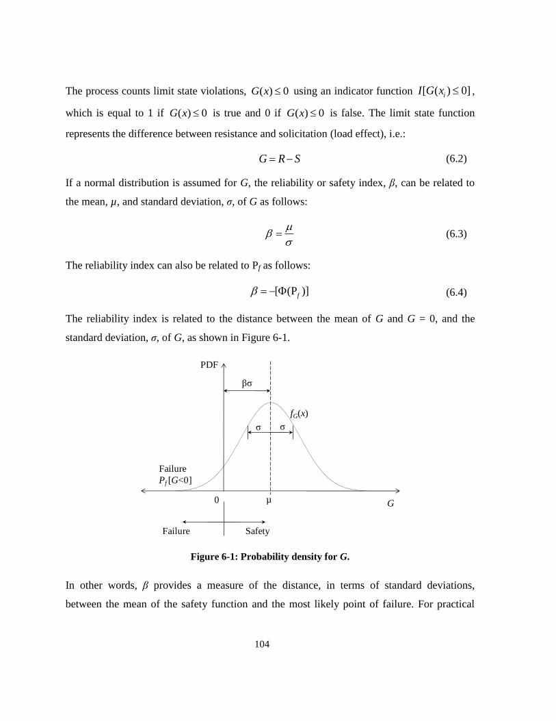
104
The process counts limit state violations, ( ) 0G x
using an indicator function [ ( ) 0]iI G x ,
which is equal to 1 if ( ) 0G x
is true and 0 if ( ) 0G x is false. The limit state function
represents the difference between resistance and solicitation (load effect), i.e.:
G R S (6.2)
If a normal distribution is assumed for G, the reliability or safety index, β, can be related to
the mean, µ, and standard deviation, σ, of G as follows:
(6.3)
The reliability index can also be related to Pf as follows:
[ (P )]f (6.4)
The reliability index is related to the distance between the mean of G and G = 0, and the
standard deviation, σ, of G, as shown in Figure 6-1.
Figure 6-1: Probability density for G.
In other words, β provides a measure of the distance, in terms of standard deviations,
between the mean of the safety function and the most likely point of failure. For practical
G
Failure Safety
Failure
Pf [G<0]
σ σ
fG(x)
βσ
µ0

105
use, CAN/CSA S6-06 tabulates the relationship between the reliability index and probability
of failure (see Table 6.1).
Table 6.1: Relationship between probability of failure and reliability index (CAN/CSA S6).
Reliability index, β Notional probability of failure, pf
2.0 2.3 × 10⁻²
or 1:44
2.5 6.2 × 10⁻³
or 1:160
3.0 1.4 × 10⁻³
or 1:740
3.5 2.3 × 10⁻⁴
or 1:4 300
4.0 3.2 × 10⁻⁵
or 1:31 500
4.5 3.4 × 10⁻⁶
or 1:294 000
The reliability index, of course, can be compared to the target index computed in accordance
with CSA/CAN S6-06 as discussed in Section 3.6.1. The target index is generally based on
acceptable degrees of risk to the general public as shown in Table 6.2.
Table 6.2: Acceptable degree of risk in society (MacGregor 1976).
Activity
Yearly death rate per person per year
For those
concerned
For the total
population
Motorcycle Racing 5 × 10⁻³
Mountain Climbing 5 × 10⁻³
Mining 7 × 10⁻⁴
Swimming 1 × 10⁻⁴
2 × 10⁻⁵
Automobile travel 3.6 × 10⁻⁴
Airplane travel 1 × 10⁻⁴
Fire in buildings 2 × 10⁻⁵
Poisoning 1.1 × 10⁻⁵
Lightning 5 × 10⁻⁷
Structural Collapse
During Construction 3 × 10⁻⁵
All others 2 × 10⁻⁷
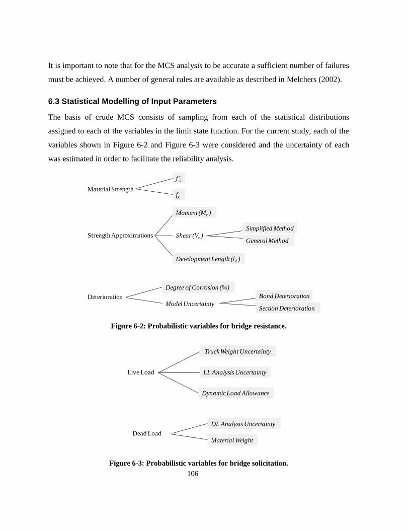
106
It is important to note that for the MCS analysis to be accurate a sufficient number of failures
must be achieved. A number of general rules are available as described in Melchers (2002).
6.3 Statistical Modelling of Input Parameters
The basis of crude MCS consists of sampling from each of the statistical distributions
assigned to each of the variables in the limit state function. For the current study, each of the
variables shown in Figure 6-2 and Figure 6-3 were considered and the uncertainty of each
was estimated in order to facilitate the reliability analysis.
Figure 6-2: Probabilistic variables for bridge resistance.
Figure 6-3: Probabilistic variables for bridge solicitation.
Material Strength
Strength Approximations
Deterioration
f‘c
fy
Moment (Mr )
Shear (Vr )
Development Length (ld )
Simplified Method
General Method
Degree of Corrosion (%)
Model Uncertainty
Bond Deterioration
Section Deterioration
Live Load
Dead Load
Truck Uncertainty
LL Analysis Uncertainty
DLA
DL Analysis Uncertainty
Material Weight
Live Load
Dead Load
Truck Uncertainty
LL Analysis Uncertainty
DLA
DL Analysis Uncertainty
Material Weight
Dynamic Load Allowance
Truck Weight Uncertainty

107
Reliability analysis requires uncertainties to be estimated for each variable. The assumed
statistical properties for the bias factors associated with each variable are shown in Table 6.3.
Table 6.3: Bias Factors for probabilistic analysis.
Uncertainty Description Bias Factor
Dist. Type Mean CoV Source
Lo
ad
ing
Live
LL Annual Extreme Event
(Moment) Gumbel 1.247 0.058 [CSA-S6 Calib.]
LL Annual Extreme Event
(Shear) Gumbel 1.285 0.059 [CSA-S6 Calib.]
LL Analysis Normal 0.93 0.12 [CSA-S6 Calib.]
DLA Normal 1.1 0.072 [CSA-S6 Calib.]
Dead Self Weight Normal 1.05 0.1 [CSA-S6 Calib.]
DL Analysis Normal 0.93 0.12 [CSA-S6 Calib.]
Res
ista
nce
(R
)
Material
Strength (M)
f'c Normal 1.25 0.131 [Bartlett and
MacGregor 1994]
fy Lognormal 1.115 0.1 [Cheung and Li 2002]
Professional
Factor (P)
Moment (Mr) Normal 1.14 0.13 [Nowak and Szerszen
1998]
Shear (Simplified) Normal 1.34 0.176 [Bentz 2010]
Shear (General) Normal 1.19 0.129 [Collins et al. 2008]
Development Length (Ld) Normal 0.785 0.161 [modified Rezansoff
and Sparling 1996]
Deterioration
(D)
Degree of Corrosion
Model for Bond
Deterioration
Model for Section Loss
The parameters for deterioration (D) are still under investigation. At this time, the analysis
does not consider cross section loss and bond deterioration due to corrosion. A sample input
file for the reliability analysis is shown in Appendix D-1.
6.3.1 Statistical Resistance Modelling
The resistance of a structure, R, is defined by Nowak and Grouni (1994) as being made up of
nominal resistance, Rn, multiplied by the uncertainty involved in the material properties, M,
fabrication (geometry), F, and a professional/analysis factor, P.
nR R M F P (6.5)
108
At this point, fabrication errors (and geometric variations) are ignored. Since geometric
variations factor into both resistance and load effects they may have a cancelling effect. The
variability in bar sizes is generally small (Melchers 2002) and therefore omitted from the
current study. Likewise, to simplify the analysis, the spatial variations of each parameter
have not been modelled in this analysis thus far. In this section the selection of each
parameter distribution is discussed.
Concrete Strength
The uncertainty associated with the concrete compressive strength according to Cheung and
Li (2002) has a bias (mean) of 0.805 and coefficient of variation (COV) of 15% with a
lognormal distribution. Based on Melchers (2002), these values appear to be reasonable and
generally at the lower end of relevant work. However, it is expected that these commonly
used factors do not capture the difference between specified and delivered concrete strengths,
but rather compare batches of cylinders of constant mix design. In an extensive report,
Bartlett and MacGregor (1994) studied in situ cores taken from structures built in Alberta
between 1988 and 1993 and found the average in situ strength to be 1.2 times the specified
strength (for shallow structure depths) with a COV of 18.6%. They noted that the data was
normally distributed. This value captures and encompasses variations in batch and location
strengths. Bailey (1996) suggests a bias of 1.28 and 11% COV for in situ concrete. It is
important to note that quality control varies significantly around the world and throughout
history. For this Canadian study, the values by Barlett and MacGregor (1994) were selected.
Steel Strength
Cheung and Li (2002) suggest reinforcing steel has a strength ratio bias of 1.115 with a CoV
of 10%. Mirza and MacGregor (1982) show very good agreement to this (mean of 1.115 and
COV 6.4%). They suggest a lognormal distribution. In his analysis Bailey (1996) uses a
mean of 1.25 with a COV of 8%. The statistics presented by Cheung and Li (2002) are
representative for old steel that likely has lower strengths with higher levels of variability
resulting from poor quality control.
109
6.3.1.1 Professional Factors
Professional factors account for the difference between tested strengths and strengths
predicted using the deterministic CAN/CSA design code equations. When applied to the
reliability analysis they, in essence, remove the implicit conservatism in standard design
approximations.
It is important to note, at this point, that when test-to-predicted values are used to derive a
professional factor, it is implicitly assumed that the tests are perfectly accurate. That is
geometric variations and concrete strengths are consistent between test specimens and the
computation of predicted values. Herein, this assumption has been made and test-to-predicted
ratios are simply used as professional factors in which variations in material strengths and
geometric conditions are additionally applied as per Equation 6.5.
Flexure
For flexure, most current standards use a rectangular stress block as an approximation.
Nowak and Grouni (1994) recommend professional factors based on their simulation of
moment-curvature relationships with comparisons to test results. They found that the
strengths had a mean of 1.02 and COV of 6%. These values are consistent with work by
Ellingwood et al. (1980), Mirza and Mcgregor (1982) and Isreal (1986). Panesar and Bartlett
(2006) suggest strain hardening increases test results by 16%. Based on these values, a mean
of 1.18 (1.02+0.16) may be justified, but relies on the assumption that the member is
underreinforced to be accurate. Factors by Nowak and Szerszen (1998) with a mean of 1.14
and CoV of 135 are used herein.
Shear General Method
For establishing the CAN/CSA A23.3 General Method for shear design, Collins et al. (1996)
compared test-to-predicted strengths of 580 beam specimens. They found the ratio had a
mean of 1.39 and COV of 0.197. However, the General Method has evolved significantly
since then. These statistics were confirmed by Somo and Hong (2006) using the computer

110
program Response 2000 (based on the modified compression field theory) to derive statistical
data with comparisons to a database of experimental shear strengths. For shear span to depth
ratios greater than two they found the program had a resistance ratio mean of 1.26 and COV
of 0.33. However, these values should stand as a lower bound since the General Method code
equations are more conservative than the program. A review of current standards by Collins
et al. (2008) examined a database of 1849 tests. They recommended the statistical
distribution to their data had a mean of 1.21 and a CoV of 15.3%. They also fitted a normal
distribution to the unconservative half of the data with a mean of 1.19 and CoV of 12.9%. It
is important to, in this case, base the analysis on the unconservative half of the data, because
there are a number of failure modes that artificially enhance shear strength and few that
artificially reduce it. The result is a skewed (conservative) distribution. Herein, the
recommendations by Collins et al (2008) were adopted for the General Method professional
factor. These factors should not be extended to span-to-depth ratios less than 2 (or 2.5) since
the code formulae do not accurately predict the strengths of deep beams (due to arch action).
It is important to note that herein the General Method is used with the modified area concept
and is an approximation. Maximum shear and flexure load effects are used. Therefore this
analysis is implicitly conservative.
Simplified Method
For the CAN/CSA Simplified Method, Polak and Dubas (1996) suggest a mean of 1.12 and a
COV of 0.19, but this work was based on CAN/CSA A23.3-M94 standards. Sun (1999)
suggests a mean of 1.26 and COV of 0.246 using another database of test results. Sun
suggests a normal or Gumbel distributions. Somo and Hong (2006) suggest a mean of 1.43
and COV of 0.43 after analyzing their database of results. Most recently, Bentz (2010)
analyzed a database of tests using three accuracy levels. The least of these corresponded to
the CAN/CSA Simplified Method. He found the data on the unconservative half was
normally distributed with a mean of 1.34 and a coefficient of variation of 17.6%.
111
Development Length
The CAN/CSA A23.3 computation of development length is based on ACI Committee 408.
An evaluation by Rezansoff and Sparling (1995) of tension lap splices found small
differences between the two in overall prediction accuracies. A Report by ACI Committee
408 (ACI 408R-03) suggests its formulae have a test-to-predicted ratio mean of 1.284 and
COV of 0.135. Rezansoff and Sparling (1996) however found that the strength ratio has a
mean of 1.46 (0.161 COV) and 1.54 (0.203 COV) for CSA 23.3 and ACI 408, respectively.
This analysis uses CAN/CSA A23.3-04 for development. Therefore, a normal distribution
was assumed with a bond-strength ratio mean of 1.46 and COV of 0.161. The required
development length is inversely related to the strength. Therefore, for development, a mean
of 1/1.46 = 0.685 was selected. A CRSI report (2001) suggests adding 10% to development
lengths for vintage steel bars as a good rule of thumb. Therefore, the required development
length was varied normally about a mean of 0.785 with a COV of 0.161.
6.3.2 Statistical Solicitation (i.e. Load) Modelling
The uncertainty in the dead load is the result of variations in the self weight and the structural
analysis method used. For the current analysis, a simple 2-D SAP 2000 frame was used, but
the transverse analysis was completed using CAN/CSA S6-06. For this case, the CAN/CSA-
S6 Calibration report suggests the factors listed in Table 3.7 for simplified code methods, and
the self-weight uncertainty associated with cast-in-place components.
Extreme event statistics were calculated using the approach described in the CAN/CSA-S6
Calibration Report using annual truck data. The report relied on data with a sample size of
13391 trucks, driven over bridges of varying length. They develop Gumbel distributions for
each traffic class, as defined by the average daily truck traffic or ADTT. For this analysis, it
has been assumed that the bridge supports an ADTT of 500 trucks (less than the design Class
A Highway).
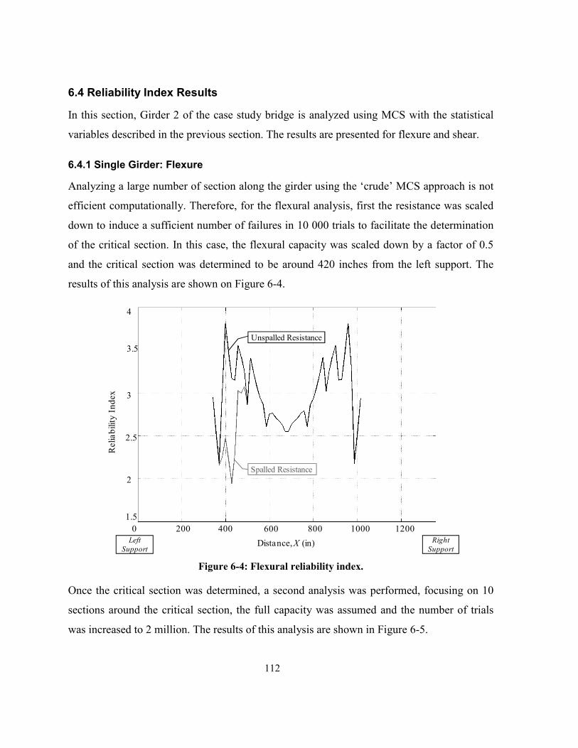
112
6.4 Reliability Index Results
In this section, Girder 2 of the case study bridge is analyzed using MCS with the statistical
variables described in the previous section. The results are presented for flexure and shear.
6.4.1 Single Girder: Flexure
Analyzing a large number of section along the girder using the ‘crude’ MCS approach is not
efficient computationally. Therefore, for the flexural analysis, first the resistance was scaled
down to induce a sufficient number of failures in 10 000 trials to facilitate the determination
of the critical section. In this case, the flexural capacity was scaled down by a factor of 0.5
and the critical section was determined to be around 420 inches from the left support. The
results of this analysis are shown on Figure 6-4.
Figure 6-4: Flexural reliability index.
Once the critical section was determined, a second analysis was performed, focusing on 10
sections around the critical section, the full capacity was assumed and the number of trials
was increased to 2 million. The results of this analysis are shown in Figure 6-5.
0 200 400 600 800 1000 1200
Distance, X (in)
Rel
iabi
lity
Inde
x
Spalled Resistance
Unspalled Resistance
Left
Support
Right
Support
1.5
2.5
3.5
2
3
4

113
Figure 6-5: Reliability Index determined by MCS analysis at critical section.
In this analysis, at the critical section a minimum reliability index of 3.973 was calculated.
Therefore, this value is the lower bound reliability of the girder analysed.
Section 3.6 of this thesis proposes an approximate reliability analysis, based on CAN/CSA
S6. The results of the MCS analysis and approximate analysis are both summarized on Table
6.4 and compared graphically in Figure 6-6.
Table 6.4: Critical section in flexure reliability: Analysis summary.
Analysis Exposure Min. R.I. Location Failures
(in 2····106 trials)
Approx. Analysis Unspalled 6.86 979.2 N/A Spalled 5.961 377.8 N/A
MCS Analysis Unspalled 3.994 374.5 65 Spalled 3.973 429.5 71
200 400 600 800 1000 1200
Rel
iabi
lity
Inde
x
Distance, X (in)
Spalled ResistanceUnspalled Resistance
3.9
4.1
4.3
4.5
4.7
0Left
Support
Right
Support
Analysis Range

114
Figure 6-6: MCS vs. approximate reliability analysis for flexure.
The results indicate an approximate-to-actual ratio of 1.50. Although the general trends are
similar for both models, the approximate method is unconservative. It is expected that, in
reality, the MCS is detecting and including additional sources of uncertainty that the
approximate method doesn’t. These might include conservatism in the development length
calculation and discrepancy between load or resistance factors and the actual statistical data
for each. In addition, the simplified method assumes normal distributions for each load effect
component. These are varied for the Monte-Carlo simulation.
6.4.2 Single Girder: Shear Simplified Method
The MCS analysis was repeated for the simplified shear method presented in Section 3.5.2.
Sufficient failures were reached within 100,000 trials analysed at 100 sections along the
girder length and, as a result, scaling of either the load effect or capacity was not required.
The probabilities of failure and reliability indices determined by this analysis are presented in
Figure 6-7 and Figure 6-8, respectively.
Approx. Method
Full Analysis
0
4
8
12
16
0 200 400 600 800 1000 1200
Rel
iabi
lity
Inde
x
Distance, X (in)Left
Support
Right
Support
Full Analysis
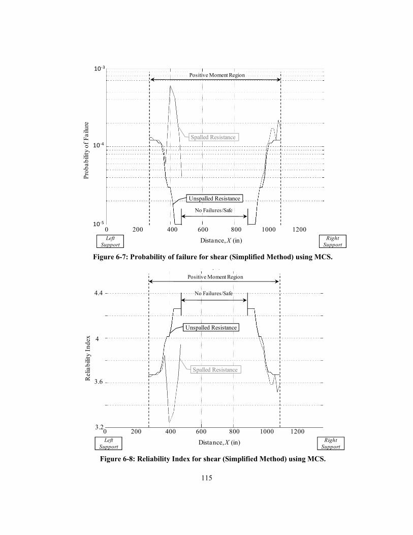
115
Figure 6-7: Probability of failure for shear (Simplified Method) using MCS.
Figure 6-8: Reliability Index for shear (Simplified Method) using MCS.
Spalled Resistance
Unspalled Resistance
Prob
abili
ty o
f Fa
ilure
Distance, X (in)Left
Support
Right
Support
No Failures/Safe
Positive Moment Region
10-5
10-4
10-3
200 400 600 800 1000 12000
Spalled Resistance
Unspalled Resistance
Rel
iabi
lity
Inde
x
Distance, X (in)Left
Support
Right
Support
No Failures/Safe
Positive Moment Region
3.2
3.6
4
4.4
200 400 600 800 1000 12000

116
A minimum reliability index of 3.239 was simulated by MCS at the critical section. A clear
distinction between the spalled and unspalled analyses is apparent. Again, the results for the
critical section analysis are summarized in Table 6.5.
Table 6.5: Critical section in shear (Simplified Method) reliability: Analysis summary.
Analysis Exposure Min. R.I. Location Failures
(in 105 trials)
Approx. Analysis Unspalled 4.54 1017 N/A
Spalled 3.40 416.3 N/A
MCS Analysis Unspalled 3.673
270-313 & 1044-1087
12
Spalled 3.239 398.9 60
Comparing the results, the approximate-to-actual analysis ratio is approximately 1.05 and the
location of the critical section appears to be very well estimated. Figure 6-9 directly compares
the MCS and approximate analysis with very good correlation observed.
Figure 6-9: Full vs. approximate reliability analysis for Simplified Shear Method.
Full Analysis
0
4
8
10
0 200 400 600 800 1000 1200
Rel
iabi
lity
Inde
x
Distance, X (in)Left
Support
Right
Support
Positive Moment Region
Approx. Method

117
6.4.3 Single Girder: Shear General Method
Finally, the analysis was repeated for the General Method for shear design proposed in
Section 3.5.3. Once again, the resistance had to be scaled down to induce failures and
identify the critical section. For this analysis, as shown in Figure 6-10, the capacity was
scaled down by a factor of 0.3.
Figure 6-10: Shear (General Method) reliability index.
Focusing the analysis on the identified critical locations did not improve the simulation and
the result was zero failures in 2 million trials. The analysis was abandoned on the basis that
the reliability index was greater than 4.89 (the index corresponding to one failure in two
million trails) since no failures occurred on the simulations of this size.
Table 6.6: Critical section in shear (General Method) reliability analysis summary.
Analysis Exposure
Min. R.I. Location Failures
(in 2····106 trials)
Approx. Analysis Unspalled 3.96 262.4 N/A Spalled 3.96 262.4 N/A
Full Analysis A Unspalled >4.89 1096 0 Spalled >4.89 261.3 0
Spalled Resistance
Rel
iabi
lity
Inde
x
Distance, X (in)Left
Support
Right
Support
No Failures/Safe
Positive Moment Region
Unspalled Resistance
1
2
3
4
0 200 400 600 800 1000 1200
118
In fact, the approximate analysis does a good job of suggesting a high index for this case but
fails to accurately predict the reliability index.
6.4.4 Single Girder: Total Reliability
The reliability of this girder is governed by shear. Overall, the approximate method estimated
the index within an Approximate:Actual analysis ratio of 1.05. From this MCS analysis, the
reliability index determined (3.239) is less than the target reliability index of 3.5 calculated in
Section 3.6.1 using CSA/CAN-S6.06. Likewise, the approximate analysis prediction of 3.4 is
consistent with the MCS index and does not meet this target. Interestingly, for the unspalled
girder, the index (3.67) exceeds the target and therefore when longitudinal reinforcement is
exposed this girder can be deemed insufficient due to the deterioration.
It should be noted, however, that theoretically, both shear methods should generate equal
reliability indices. It is concluded that the reliability analysis based on the General Method
needs to be further examined to find an exploration for this discrepancy.
In a practical sense, a deterministic approximation of the reliability index may be more useful
than one based on the approximate reliability analysis. Such an approximation would allow
an evaluator to use a reliability index for comparisons between structures and the target index
defined by CSA/CAN S6-06. Repairs and replacements could be prioritized based on this
index and a limiting criterion. In Figure 6-11, the results of the full reliability analysis are
compared to the deterministic resistance ratio (resistance ÷ load effect). There appears to be a
linear relationships between the resistance ratio and reliability index for both flexure and
shear (based on the Simplified Method for the shear design).

119
Figure 6-11: Resistance ratio and reliability index for flexure and shear.
The relationship may also be consistent enough for a single relationship to represent both
flexural and shear results as shown in Figure 6-12.
Figure 6-12: Resistance ratio and reliability index for both analyses.
y = 0.291x + 0.0212
y = 0.1339x + 0.9782
0
0.2
0.4
0.6
0.8
1
1.2
1.4
1.6
1.8
3 3.5 4 4.5 5
Res
ista
nce
Rat
io
Reliability Index
Shear
Flexure
y = 0.4889x - 0.6619
0
0.2
0.4
0.6
0.8
1
1.2
1.4
1.6
1.8
3 3.5 4 4.5 5
Res
ista
nce
Rat
io
Reliability Index

120
The presented analysis is only for Girder 2. To establish an empirical relationship that can be
used for a wider range of structure configurations, loading conditions and spalling scenarios,
a larger number of comparisons are required.

121
Chapter 7
Conclusions and Recommendations
7.1 Conclusions
The conclusions presented in this chapter were drawn from: (1) the deterministic analysis
presented in Chapters 3 and 4, (2) the laboratory study presented in Chapter 5, and, (3) the
probabilistic (reliability) analysis presented in Chapter 6 of this thesis.
7.1.1 Deterministic Analysis
Based on the deterministic analysis presented herein, the following conclusions are drawn:
When sections of reinforced concrete (RC) bridge girder reinforcement are exposed,
development becomes critical and in many cases the required development length
may no longer be provided.
For the investigated case study bridge, the remaining structural capacity is directly
related to the spatial distribution of the spalling relative to bar cutoffs and splices.
The modified area concept offers a viable method for estimating an RC girder‘s
flexural or shear strength when full development is no longer provided.
A multi-point analysis program, employing the modified area method, offers a viable
tool for the rapid assessment of spalled RC bridge girders.
In general, the consideration of system effects improves the bridge condition
estimate, since the spalled regions will generally vary from one girder to the next.
The proposed full bridge analysis utilized by the program BEST efficiently considers
system effects and strength deficiencies that arise from adjacent deteriorated RC
girders, considering the pattern of deterioration across the structure.

122
Rebar section loss and bond deterioration can also be considered in the analysis by
incorporating existing empirical models of these effects. In general, lower calculated
resistance ratios will result when these effects are included in the analysis.
7.1.2 Laboratory Work
The following conclusions were drawn from the pilot laboratory study:
The BEST computer program provides accurate (and conservative) estimates for the
strength of the test specimens with exposed reinforcement.
The symmetry of spalling (or lack thereof) along a beam or about a point of loading
likely does not affect the strength if development length is compromised.
If development is provided, arch action can create a shift from shear failure to
concrete crushing. High ductility can provide adequate warning of failure.
Intact sections centred under the load point may act like a pivot and do not fully
contribute to bond. On real bridges, symmetric spalling is improbable and under a
moving truck load these sections may engage when the truck is in other positions.
Intact sections with a length and depth of spalling resulting in premature local shear
failure (such as Beam 6) can only be partially counted on for bond. As a conservative
estimate, these sections may be ignored. Further work is required to establish length
limits for unspalled sections to be considered in the development length calculation
that could be implemented in the BEST computer program.
Both SikaTop 123 and Sikacrete-08 SCC appear to effectively restore bond and
member strength over spalled sections.
When spalled region repairs are applied to a relatively weak substrate concrete, the
increase in tension stiffening can result in increased member stiffness.
123
7.1.3 Reliability Analysis
The following conclusions were drawn from the reliability analysis:
Statistical parameters were derived for the probabilistic evaluation of any RC bridge.
This analysis uses statistical distributions as professional factors associated with
CAN/CSA code equations for flexure, shear, and development length in a
probabilistic study.
Based on comparisons with the Monte-Carlo analysis, the approximate reliability
analysis presented herein, appears to provide a viable estimate of the reliability of a
spalled bridge structure deterministically.
With a broader range of studies, an empirical relationship between the deterministic
resistance ratio and the reliability index may be established. A formula based on the
deterministic resistance ratio such as the one presented herein could allow bridge
evaluators to quickly assess and compare structures, prioritizing repairs and
replacements based on the deterministic reliability index.
7.2 Recommendations for Future Work
To further advance this field of the study, a number of possibilities have been identified.
7.2.1 Further Development of BEST Computer Program
The BEST computer program presented herein requires further development, before it can be
considered an industry-ready tool. The following advancements are recommended:
To evaluate the potential of the program, a multi-span conventionally RC bridge with
spalling could be analyzed using the existing program. A number of critical sections
could arise for such a structure if concrete surrounding the soffit steel is removed or
deteriorated.

124
At this time, the program does not consider the combined influence of axial load and
flexure that occurs in rigid frame structures (such as the case study structure). In this
regard, it is conservative. Code provisions for considering combined load effects,
including axial load, can easily be added to the current program, however
The models for the effects of corrosion on bond strength and section loss can also be
improved. For example, analytical models for the rebar bond strength in cracked
concrete could be modified with corrosion parameters to better predict the bond
strength between rebar and corroded concrete in intact sections.
The program could be adapted to analyze 2-way slab or prestressed concrete bridges.
Finally, a graphical user interface can easily be developed for the program. Easy to
use displays for input fields would increase the appeal of the program to potential
users.
7.2.2 Extension of Laboratory Studies
The BEST computer program should be further validated by expanded laboratory
investigations. In the next round of laboratory testing, the following could be studied:
Separate sets of flexure and shear sensitive beams should be designed. Simply
comparing the strengths of spalled specimens with different levels of transverse
reinforcement should indicate the role (if any) of transverse reinforcement on the
strength of a beam with development deficiencies.
The statistical significance of the results for each spalling configuration should be
confirmed by expanding the number of test specimens. Ideally, specimens could be
designed to reduce the impact of confining stress above supports. For example a
splice within the span may be used to remove this source of inaccuracy.
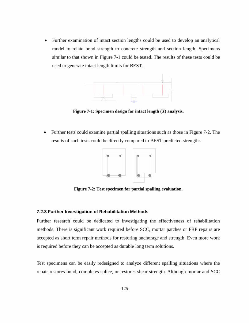
125
Further examination of intact section lengths could be used to develop an analytical
model to relate bond strength to concrete strength and section length. Specimens
similar to that shown in Figure 7-1 could be tested. The results of these tests could be
used to generate intact length limits for BEST.
Figure 7-1: Specimen design for intact length (X) analysis.
Further tests could examine partial spalling situations such as those in Figure 7-2. The
results of such tests could be directly compared to BEST predicted strengths.
Figure 7-2: Test specimen for partial spalling evaluation.
7.2.3 Further Investigation of Rehabilitation Methods
Further research could be dedicated to investigating the effectiveness of rehabilitation
methods. There is significant work required before SCC, mortar patches or FRP repairs are
accepted as short term repair methods for restoring anchorage and strength. Even more work
is required before they can be accepted as durable long term solutions.
Test specimens can be easily redesigned to analyze different spalling situations where the
repair restores bond, completes splice, or restores shear strength. Although mortar and SCC
X

126
products restored bond and strength on the beams tested, they did not complete a splice.
Specimens, such as that shown in Figure 7-3, represent a more realistic case.
Figure 7-3: Proposed detail for splice repair evaluation.
A potential area of concern is the durability of patch materials. Repair materials are often
subject to rapid deterioration due to corrosion, accelerated by corrosion products cast or
trapped within the repair, and extensive cracking. Often high strength repairs show extensive
flexural cracking as well as cracking relative to the substrate material due to material
property differentials.
7.2.4 Improvements in Corrosion Measurement
There currently is a shortage of quick, useful methods for measuring corrosion effects on RC
structures. For the BEST computer program to be a realistic representation of the corroded
strength of a deteriorated bridge, there needs to be improved means of accurately
approximating the degree of corrosion in-situ. The following potential avenues could be
explored:
Within spalled sections, if the corrosion appears to be uniform, then potentially a
caliper can accurately measure the degree of corrosion. Field trials could be compared
to extracted samples measured in the lab using the displaced water technique. If
pitting corrosion is evident, then a dial gauge similar to the one proposed
conceptually in Figure 7-4 may be useful.
Evaluate Patch RepairsPatch Repair

127
Figure 7-4: Concept for reinforcement corrosion pit gauge.
For corrosion levels less than 10% section loss (due to accuracy concerns) perhaps,
Nondestructive testing (NDT) methods such as ground penetrating radar (GPR) or
eddy current techniques could be explored.
For intact sections, a study could examine test specimens artificially corroded to
relate the degree of corrosion with the first appearance of longitudinal cracking or
crack width. Surface staining could be another clue to the degree of corrosion within
intact sections.
An alternative study could examine the degree of corrosion on sections taken from a
decommissioned structure or a structure recently scaled in an attempt to relate the
level of corrosion within intact sections to that of exposed reinforcement as a function
of the amount of time the steel has been exposed.
Figure 7-5: Corrosion cracking, surface staining and section loss.
7.2.5 Effect of Corrosion on Other Components
There are legitimate concerns about the impact of corrosion on parts of the structure other
than girder soffits. MTO officials have highlighted significant concerns about slab spalling.
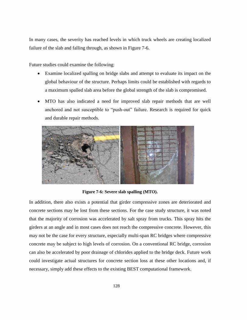
128
In many cases, the severity has reached levels in which truck wheels are creating localized
failure of the slab and falling through, as shown in Figure 7-6.
Future studies could examine the following:
Examine localized spalling on bridge slabs and attempt to evaluate its impact on the
global behaviour of the structure. Perhaps limits could be established with regards to
a maximum spalled slab area before the global strength of the slab is compromised.
MTO has also indicated a need for improved slab repair methods that are well
anchored and not susceptible to ―push-out‖ failure. Research is required for quick
and durable repair methods.
Figure 7-6: Severe slab spalling (MTO).
In addition, there also exists a potential that girder compressive zones are deteriorated and
concrete sections may be lost from these sections. For the case study structure, it was noted
that the majority of corrosion was accelerated by salt spray from trucks. This spray hits the
girders at an angle and in most cases does not reach the compressive concrete. However, this
may not be the case for every structure, especially multi-span RC bridges where compressive
concrete may be subject to high levels of corrosion. On a conventional RC bridge, corrosion
can also be accelerated by poor drainage of chlorides applied to the bridge deck. Future work
could investigate actual structures for concrete section loss at these other locations and, if
necessary, simply add these effects to the existing BEST computational framework.

129
Bibliography
ACI Committee 222. 1988. Corrosion of metal in concrete. American Concrete Institute
manual of concrete practice: Part 1. Detroit, USA, ACI 222R-85.
Al-Sulaimani, K., Basunbul M., and Rasheeduzzafar, I.A.1990. Influence of corrosion and
cracking on bond behaviour and strength of reinforced concrete members. American
Concrete Institute Structural Journal, 87(2): 220–231.
Amey, S. L., Johnson, D. A., Miltenberger, M. A., and Farzam, H. 1998. Temperature
dependence of compressive strength of conversion-inhibited high alumina cement
concrete. American Concrete Institute Structural Journal, 95(1): 27-36.
Andrade, C. 1993. Calculation of chloride diffusion coefficients in concrete from ionic
migration measurements. Cement and Concrete Research, 23(3): 724–742.
Andrade, C., Alonso, C., Garcia, D., and Rodriguez, J. 1991. Remaining lifetime of
reinforced concrete structures: effect of corrosion in the mechanical properties of the steel.
In Proceedings of the International Conference on Life Prediction of Corrodible
Structures, Cambridge, UK., 23-26 September 1991. National Association of Corrosion
Engineers. pp. 12/1-12/11.
Auditor general report, 2009. 3.02 Bridge inspection and maintenance, Office of the Auditor
General of Ontario. December 7 2009.
Azam, R. 2010. Behaviour of Shear Critical RC Beams with Corroded Longitudinal Steel
Reinforcement. M.Sc. thesis, Department of Civil and Environmental Engineering, The
University of Waterloo, Waterloo, Ont.
Bailey, S.F. 1996. Basic principles and load models for the structural safety evaluation of
existing road bridges. Ph.D. Thesis No. 1467, École Polytechnique Fédérale de Lausanne,
Switzerland.
Ballim, Y. and Reid, J.C. 2002. Reinforcement corrosion and the deflection of RC beams -
an experimental critique of current test methods. Cement and Concrete Composites,
25(6):635-632.
Bartlett, M. 2010. Behaviour of Partially-Repaired Reinforced Concrete T-Beams.
Unpublished.
Bartlett, M.F. and MacGregor. J.G. 1994. Assessment of concrete strength in existing
structures. Structural Engineering Report No. 198. University of Alberta, May 1994.

130
Bazant, Z. P. 1979. Physical model for steel corrosion in concrete sea structures-theory.
ASCE Journal of Structural Division, 105(6): 1137–1153.
Bentz, E.C. 2010. MC2010: Shear strength of beams and implications of the new approaches.
In FIB/CEB Bulletin 57: Shear and punching shear in RC and FRP Elements, Proceedings
of an International Conference, Salo, Italy, 15–16 October 2010, pp. 15–31.
Bentz, E. 2006. Summary of Development and Use of CSA 2004 Shear Design Provisions. In
Advances in Engineering Structures, Mechanics. Edited by M. Pandey et al. Springer,
Netherlands. pp. 67-80.
Berto, L., Simioni, P. and Saetta, A. 2008. Numerical modelling of bond behaviour in RC
structures affected by reinforcement corrosion. Engineering Structures, 30(5): 1375–1385.
Bhargava, K., Ghosh, A.K., Mori, Y., and Ramanujam, S. 2007. Corrosion-induced bond
strength degradation in reinforced concrete - analytical and empirical models. Nuclear
Engineering and Design, 237(11): 1140-1157.
Cabrera, J.G. 1996. Deterioration of concrete due to reinforcement steel corrosion. Cement
and Concrete Composites, 18(1): 47–59.
Cabrera, J.G., and Ghoddoussi, P. 1992. The effect of reinforcement corrosion on the
strength of the steel concrete bond. In Proceedings of the International Conference on
Bond in Concrete, Riga, Latvia, 15-17 October 1992. pp. 10/11–10/24.
Cairns, J. and Abdullah, R.B. 1996. Bond strength of black and epoxy-coated
reinforcement—a theoretical approach, ACI Materials Journal, 93(4): 362–369.
Cairns, J. and Zhao, Z. 1993. Behaviour of concrete beams with exposed reinforcement. In
Proceedings of the Institution of Civil Engineers – Structures and Buildings, 99(2) May
1993. Institution of Civil Engineers, London, UK, pp. 141-154.
Cairns, J., Du, Y.G. and Law, D. 2005a. Criteria for and prediction of limit states of
degradation of reinforced concrete structures. In Proceedings of 6th International
Conference: Global Construction: Ultimate Concrete Opportunities, Dundee, UK, 5-7 July
2005.
Cairns, J., Plizzari G., Du, Y.G., Law, D.W., and Franzoni, C. 2005b. Mechanical properties
of corrosion damaged reinforcement. American Concrete Institute Structural Journal,
102(2): 256-264.

131
Cairns, J., Du, Y.G. and Law, D. 2008. Structural performance of corrosion-damaged
concrete beam. Magazine of Concrete Research, 60(5): 359-370.
Canadian Standards Association. 2004. CSA Standard A23.3-04: Design of Concrete
Structures. Mississauga, O.N.
Canadian Standards Association. 2006. CAN/CSA S6-06: Canadian Highway Bridge Design
Code. Mississauga, O.N.
Canadian Standards Association. 2007.Calibration report for CAN/CSA-S6-06: Canadian
highway bridge design code.
Cheung, M.S. and Li, W.C. 2002. Reliability assessment in highway bridge design. Canadian
Journal of Civil Engineering, 29:799-805.
Chung, L., Cho, S.H., Kim, J.H.J., and Yi, S.T. 2004. Correction factor suggestion for ACI
development length provisions based on flexural testing of RC slabs with various levels of
corroded reinforcing bars. Engineering Structures, 26(8): 1013–1026.
Clark, L.A., and Saifullah, M. 1994. Effect of corrosion rate on the bond strength of corroded
reinforcement, In Corrosion and Corrosion Protection of Steel in Concrete, Edited by R.
N. Swamy, Sheffield Academic Press, Sheffield, UK. pp. 591-602.
Collins, M.P., Bentz, E.C. and Sherwood, E.G. 2008. Where is shear reinforcement required?
Review of research results and design procedures. ACI Structural Journal, 105(5), 590-
600.
Collins, M.P., Mitchell, D., Adebar, P.E. and Vecchio, F. J. 1996. A general shear design
method. ACI Structural Journal, 93(1): 36-45.
Comite Eurointernational du Beton (CEB), Federation Internation du Beton (FIB), 2000.
Bond of Reinforcement in Concrete: State-of-Art, Bulletin No. 10.
Coronelli, D. 2002. Corrosion cracking and bond strength modeling for corroded bars in
reinforced concrete. American Concrete Institute Structural Journal, 99(3): 267–276.
Council of the Federation, 2005. Looking to the Future: A Plan for Investing in Canada's
Transportation System [online]. Available from www.councilofthefederation.ca/ [cited
April 27 2011].
CRSI. 2001. Evaluation of reinforcing bars in old reinforced concrete structures. Engineering
Data Report Number 48. Concrete Reinforcing Steel Institute.
132
Du, Y. 2001. Effect of Reinforcement Corrosion on Structural Concrete Ductility. PhD
thesis, Department of Civil Engineering, University of Birmingham, Birmingham, UK.
Ellingwood, B.R., Galambos, T.V., MacGregor, J.G. and Cornell, C.A. Development of a
probability-based load criterion for American National Standard A58. National Bureau of
Standards Special Publication 577, US Government Printing Office, Washington, DC,
1980.
El-Maadawy, T. and Soudki, K.A. 2007. A Model for Prediction of Time from Corrosion
Initation to Corrosion Cracking. Cement and Concrete Composites, 29(3): 168-175.
GEOCISA, Torroja Institute, 2001. CONTECVET: A validated user‘s manual for assessing
the residual service life of concrete structures. British Cement Association et al., Madrid,
Spain.
Hansson, C. M., Poursaee, A. and Laurent, A. 2006. Macrocell and microcell corrosion of
steel in OPC and high performance concrete. Cement and Concrete Research, 36(11):
2098–2102.
Hansson, C. M., Poursaee, A. and Jaffer, S. J. 2007. Corrosion of reinforcing bars in
concrete. Available from the Portland Cement Association, Illinois USA, R&D Serial No.
3013.
Hope, B.B. and Ip, A.K.C. 1987. Chloride corrosion threshold in concrete. American
Concrete Institute Materials Journal, 84(4): 306–314.
Israel, M. S. 1986. Probabilistic basis of partial resistance factors for use in concrete design.
Thesis. Johns Hopkins University.
Lee, H.S., and Cho, Y.S. 2009. Evaluation of the mechanical properties of steel
reinforcement embedded in concrete specimen as a function of the degree of
reinforcement corrosion. International Journal of Fracture, 157(1): 81-88.
Lee, H.S., Tomosawa, F., and Noguchi, T. 1996. Effect of rebar corrosion on the structural
performance of singly reinforced beams. In Durability of Building Materials and
Components. Edited by C. Sjostrom. E&FN Spon, London. pp. 571-580.
Lee, H.S., Noguchi, T., and Tomosawa, F. 2002. Evaluation of the bond properties between
concrete and reinforcement as a function of the degree of reinforcement corrosion.
Cement and Concrete Research, 32(8): 1313–1318.
133
Li, C., Zheng, J., Lawanwisut, W. and Melchers, R.E. 2007. Concrete delamination caused
by steel reinforcement corrosion. Journal of Materials in Civil Engineering, 19(7): 591–
600.
Liang, M.T., Lin, L.H., and Liang, C.H. 2002. Service life prediction of existing reinforced
concrete bridges exposed to chloride environment. ASCE Journal of Infrastructure
Systems, 8(3): 76–85.
Litvan, G.G., 1972. Phase Transitions of Adsorbates, IV: Mechanism of Frost Action in
Hardened Cement Paste. Journal of the American Ceramic Society, 55(1): 38-42.
MacGregor, J.G. 1976. Safety and limit states design for reinforced concrete. Canadian
Journal of Civil Engineering. 3(4):484-513.
Melchers, R. 2002. Structural reliability analysis and prediction, 2nd Edition. John Wiley &
Sons.
Mindess, S. and Young, J.F. 1981. Concrete. Prentice-Hall, Inc., Englewood, N.J.
Mirza, S.A. and MacGregor, J.G. 1982. Probabilistic study of strength of reinforced concrete
members. Canadian Journal of Civil Engineering. 9(43):1-48.
Morinaga, S. 1996. Remaining life of reinforced concrete structures after corrosion cracking.
In Durability of Building Materials and Components. Edited by C. Sjostrom. E&FN
Spon, London. pp. 127-137.
Nowak, A.S. and Grouni, H.N. 1994. Calibration of the Ontario highway bridge design code
1991 edition. Canadian Journal of Civil Engineering, 21: 25–35
Nowak, A.S. and Kulicki, J.M. 1996. New generation of U.S. bridge design codes. In
Proceedings, IABSE Colloquium in Eurocodes, Vol. 74, Delft, The Netherlands. March
1996, pp. 535-540.
Nowak, A.S. and Szerszen, M.M. 1998. Bridge load and resistance models. Engineering
Structures, 22(11), 985-990.
Palsson, R. and Mirza, M.S. 2002. Mechanical response of corroded steel reinforcement of
abandoned concrete bridge. American Concrete Institute Structural Journal, 99(2): 157–
162.
Panesar, D.K. and Bartlett, F.M. 2006. Load and resistance data for precast stringer highway
bridges. Canadian Journal of Civil Engineering. Vol. 33, pp.1368-1378.

134
Pigeon, W. and Pleau, R. 1995. Durability of Concrete in Cold Climates. Modern Concrete
Technology 4. E&FN Spon, U.K.
Poursaee, A. and Hansson, C.M. 2009. Potential pitfalls in assessing chloride-induced
corrosion of steel in conrete. Cement and Concrete Composites, 39(5):391-400.
Powers, T. C. 1945. A working hypothesis for further studies of frost resistance of concrete.
Journal of the American Concrete Institute. 16(4): 245-272.
Powers, T. C. and Helmuth, R. A. 1953. Theory of volume changes in hardened portland-
cement paste during freezing. Highway Research Board Proceedings, 32: 285-297.
Renew Ontario Website, 2009 (http://www.mei.gov.on.ca/english/infrastructure/renew/).
Rezansoff, T. and Sparling, B.F. 1995. Correlation of the bond provisions of CSA A23.3-94
with tests on tension lap splices in beams. Canadian Journal of Civil Engineering, 22(4):
755-769.
Rodriguez, J., Ortega, L., and Garcia, A. 1994. Corrosion of reinforcing bars and service life
of R/C structures: corrosion and bond deterioration. In ‗Concrete Across Borders‘,
Proceedings of an International Conference, Odense, Denmark, 22–25 June 1993, pp.
315–326.
Rodriguez, J., Ortega, L.M. and Casal, V. 1997. Load carrying capacity of concrete structures
with corroded reinforcement. Construction and Building Materials, 11(4): 239–248.
SAP 2000 Version 12. 2009. Computers and Structures, Inc. Berkeley, California USA.
Sika Canada, 2011. Product data sheets. (available from http://can.sika.com)
Somo, S. and Hong, H. P. 2006. Modeling error analysis of shear predicting models for RC
beams. Structural Safety, 28(3), 217-230.
Stanish, K., Hooton, R., and Pantazopoulou, S. 1999. Corrosion effects on bond strength in
reinforced concrete. American Concrete Institute Structural Journal, 96(6): 915–921.
Thomas, M.D.A. and Bentz, E.C. 2000. Life-365 computer program for predicting the
service life and life-cycle costs of reinforced concrete exposed to chlorides. Available
from www.masterbuilders.com/support/pageEtools [cited May 25, 2011].
Tuutti, K. 1982. Corrosion of steel in concrete. Swedish Cement and Concrete Research
Institute, Report 4-82, Stockholm, Sweden.

135
Zhang, P.S., Lu, M., and Li, X.Y. 1995. The mechanical behaviour of corroded bar, Journal
of Industrial Buildings, 25(257): 41-44.
136
Appendix A
Appendix A-1 Structural Drawings
Appendix A-2 Spalling Surveys
Appendix A-3 Repair History
Appendix A-4 Reinforcement/Spalling Superposition
Appendix A-5 Bridge Loads
Appendix A-6 Structural Capacity
Appendix A-7 Transverse Distribution
Appendix A-8 Slab Strength

Appendix A-1 Structural Drawings
137

Aug. Spalling Survey
DRAWING #
:
DRAWN BY:
DATE:
JLSept. 2 2010
1
Site
23-
170
HW
Y #
59GIRDER 10
GIRDER 9
GIRDER 8
GIRDER 7
GIRDER 6
GIRDER 5
GIRDER 4
GIRDER 3
GIRDER 2
GIRDER 1
Aug
ust 2
5, 2
009
Appendix A-2 Spalling Surveys
138
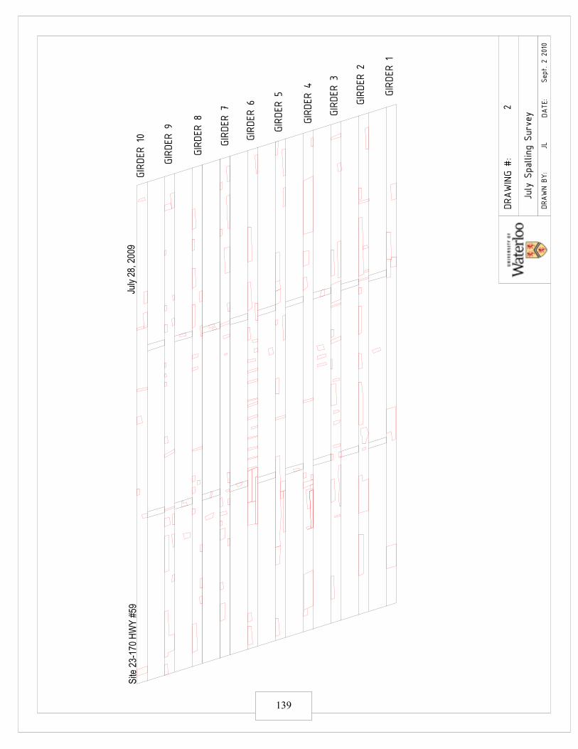
Site
23-
170
HW
Y #
59Ju
ly 2
8, 2
009
GIRDER 10
GIRDER 9
GIRDER 8
GIRDER 7
GIRDER 6
GIRDER 5
GIRDER 4
GIRDER 3
GIRDER 2
GIRDER 1
July S
palling Survey
DRAWING #
:
DRAWN B
Y:
DATE:
JLSept. 2 2010
2
139
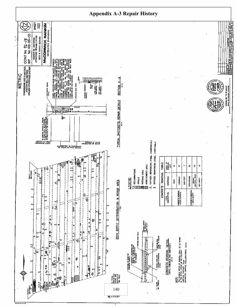
Appendix A-3 Repair History
140

'91 Repair and Current Spalling
DRAWING #
:
DRAWN BY:
DATE:
JLSept. 2 2010
3
141
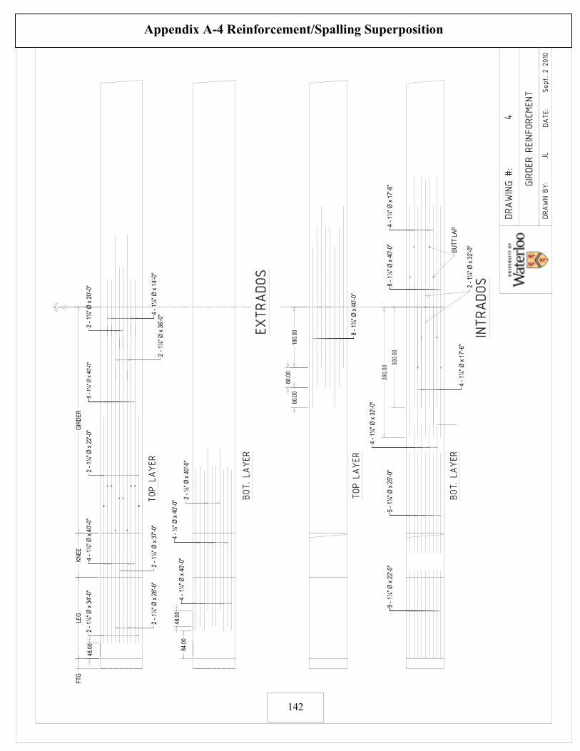
4 -
1¼"
Ø x
14'
-0"
2 -
1¼"
Ø x
34'
-0"
4 -
1¼"
Ø x
40'
-0"
2 -
1¼"
Ø x
37'
-0"
2 -
1¼"
Ø x
22'
-0"
2 -
1¼"
Ø x
28'
-0"
EXTRADOS
INTRADOS
48.0
0
84.0
048
.00
180.
0060
.00
60.0
0
GIR
DE
RK
NE
ELE
GF
TG
?
BOT. LAYER
300.
00
390.
00
BU
TT
LA
P
TOP LAYER
BOT. LAYER
TOP LAYER
9 -
1¼"
Ø x
22'
-0"
5 -
1¼"
Ø x
25'
-0"
4 -
1¼"
Ø x
32'
-0"
4 -
1¼"
Ø x
17'
-6"
8 -
1¼"
Ø x
40'
-0"
4 -
1¼"
Ø x
17'
-6"
2 -
1¼"
Ø x
32'
-0"
8 -
1¼"
Ø x
40'
-0"
2 -
½"
Ø x
40'
-0"
4 -
½"
Ø x
40'
-0"
4 -
1¼"
Ø x
40'
-0"
8 -
1¼"
Ø x
40'
-0"
2 -
1¼"
Ø x
36'
-0"
2 -
1¼"
Ø x
20'
-0"
GIRDER REINFORCMENT
DRAWING #
:
DRAWN BY:
DATE:
JLSept. 2 2010
4
Appendix A-4 Reinforcement/Spalling Superposition
142

Site
23-
170
HW
Y #
59GIRDER 10
GIRDER 9
GIRDER 8
GIRDER 7
GIRDER 6
GIRDER 5
GIRDER 4
GIRDER 3
GIRDER 2
GIRDER 1
Reinforcement-Spalling Superposition
DRAWING #
:
DRAWN B
Y:
DATE:
JLSept. 2 2010
5
143

GIRDER 2
GIRDER 1
GIRDER 4
GIRDER 5
GIRDER 6
GIRDER 7
Reinf.-Spalling Superposition for Analysis
DRAWING #:
DRAWN BY: DATE:JL Sept. 2 2010
6
GIRDER 3
GIRDER 8
GIRDER 9
GIRDER 10
144

145
Appendix A-5 Bridge Loads
CLW Truck (Cl. 3.8.3.2 Fig 3.2)
SAP2000 load envelope
Component Absolute Value
Maximum Positive Moment 7140.81 kip-in
Maximum Negative Moment 20028.4 kip-in
Maximum Shear 84.269 kip
-25000
-20000
-15000
-10000
-5000
0
5000
10000
0 500 1000
Mo
men
t (
Kip
-in
)
Distance X (in)
Unfactored Truck Moment
-100
-50
0
50
100
0 500 1000
Sh
ear
(Kip
)
Distance X (in)
Unfactored Truck Shear Envelope
Station Axel Load
m in. KN Kips
0 0 50 11.24
3.6 141.73 125 28.10
4.8 188.98 125 28.10
11.4 448.82 175 39.34
18 708.66 150 33.72
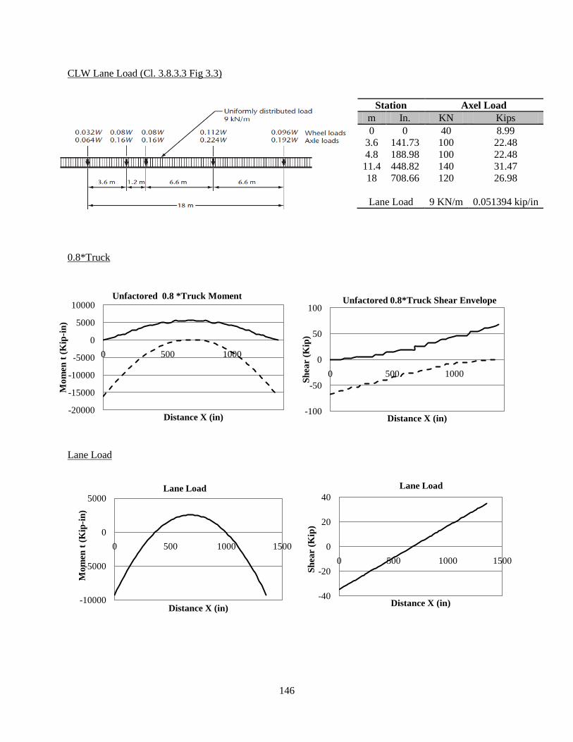
146
-100
-50
0
50
100
0 500 1000
Sh
ear
(Kip
)
Distance X (in)
Unfactored 0.8*Truck Shear Envelope
-20000
-15000
-10000
-5000
0
5000
10000
0 500 1000
Mo
men
t (
Kip
-in
)
Distance X (in)
Unfactored 0.8 *Truck Moment
CLW Lane Load (Cl. 3.8.3.3 Fig 3.3)
0.8*Truck
Lane Load
Station Axel Load
m In. KN Kips
0 0 40 8.99
3.6 141.73 100 22.48
4.8 188.98 100 22.48
11.4 448.82 140 31.47
18 708.66 120 26.98
Lane Load 9 KN/m 0.051394 kip/in
-10000
-5000
0
5000
0 500 1000 1500
Mo
men
t (
Kip
-in
)
Distance X (in)
Lane Load
-40
-20
0
20
40
0 500 1000 1500
Sh
ear
(Kip
)
Distance X (in)
Lane Load
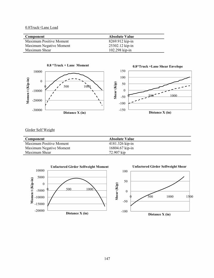
147
0.8Truck+Lane Load
Component Absolute Value
Maximum Positive Moment 8269.912 kip-in
Maximum Negative Moment 25302.12 kip-in
Maximum Shear 102.298 kip-in
Girder Self Weight
Component Absolute Value
Maximum Positive Moment 4181.326 kip-in
Maximum Negative Moment 16804.67 kip-in
Maximum Shear 72.907 kip
-30000
-20000
-10000
0
10000
0 500 1000
Momen t (Kip-in)
Distance X (in)
0.8 *Truck + Lane Moment
-150
-100
-50
0
50
100
150
0 500 1000
Shear (Kip)
Distance X (in)
0.8*Truck +Lane Shear Envelope
-20000
-15000
-10000
-5000
0
5000
10000
0 500 1000
Momen t (Kip-in)
Distance X (in)
Unfactored Girder Selfweight Moment
-100
-50
0
50
100
0 500 1000 1500
Shear (Kip)
Distance X (in)
Unfactored Girder Selfweight Shear

148
Slab Self Weight
Component Absolute Value
Maximum Positive Moment 8412.203 kip-in
Maximum Negative Moment 2318.278 kip-in
Maximum Shear 31.622 kip
-10000
-8000
-6000
-4000
-2000
0
2000
4000
0 500 1000 1500
Momen t (Kip-in)
Distance X (in)
Unfactored Slab Selfweight Moment
-40
-30
-20
-10
0
10
20
30
40
0 500 1000 1500
Shear (Kip)
Distance X (in)
Unfactored Slab Selfweight Shear

149
Appendix A-6 Structural Capacity
A-6-1 Known Information
Based on the original structure document the following information is known.
Material Property Specified Value
Concrete Compressive Strength, �′� 3000 psi (20.68 MPA)
Steel Yield Strength, �� 275 MPA
Concrete Modulus of Rupture, �� 2.729 MPA∗� Concrete Modulus of Elasticity, �� 20463 MPA∗�
�� = 4500���′ = 20463 ��� ∗� � = 0.6!���′ = 2.729 ��� ∗"
Reinforcement Diameter X-Sectional Area
inches mm in" mm" Stirrups ½ 12.7 0.1963 125.7
Bottom Lower 1 ¼ 31.75 1.227 791.73
A-6-2 Required Development Length (CAN/CSA S6.06 Highway Bridge Code)
The following computes the required development length using Canadian standards.
Clear Cover= 2 5/8 in. – 1 ¼ (0.5) = 2” (25.4) = 50.8mm
Clear Spacing= 2.44” – 1 ¼” = 1.599” (25.4) = 40.49mm
&�=1.0, &"=1.0, &'=1.0 Clear Cover= 50.8 > 31.75
Clear Spacing= 40.49 < (1.4*31.75) = 44.45mm
S = {12in , 18in} = {304.8mm , 457.2mm}, 304.8 is conservative for () . &* = 0.45 �* +,10.5 . / = 0.45 ∗ 125.7 ∗ 2 ∗ 27510.5 ∗ 304.8 ∗ 9 = 0.72568 Dcs= 2/3 * 2.844” *25.4= 48.16 mm
(Ktr + dcs)= 0.72568 + 48.16 = 48.886 < 2.5 db =79.375
() = 0.45 1�1"1'(1* + 4�5) 7 �,�� 8 �9
() = 0.4548.886 : 2750.4√20.684< 791.73 = 1109.86 mm = 43.695 in

150
A-6-3 Moment Resistance
In this section, the moment capacity of the girder is shown for a number of approximation of the section.
Accuracy is increase with each successive section. Calculations are shown for the mid-span section.
Simplified Section #1
=9>? = @ABACD′CE : FGGFGGHCE< = G.I"∗G.J�I∗"G.F"FK L FGGFGGH"FKM = 4.07%
= = OP9) = J∗FJ�.F'QQR"I∗"K.S∗'F.'I∗"K.S = 1.055%
Section is Under-Reinforced
TU = 112 Vℎ' = 112 (28 ∗ 25.4)(40 ∗ 25.4)' = 6.21X10�GYYS
�� = � TUZ* = 2.729 ∗ 6.21X10�GYYS[40 ∗ 25.42 ] = 333.6 &]. Y
^� = 0.85 − 0.0015��′ = 0.85 − 0.0015 ∗ 20.7 = 0.82 �̀ = 0.97 − 0.0025��′ = 0.97 − 0.0025 ∗ 20.7 = 0.918
a = �5�,^���′V = 9 ∗ 791.73 YY" ∗ 275 ���0.82 ∗ 20.7��� ∗ 711.2YY = 162.32 YY
� = �5�, b4 − a2c = 9 ∗ 791.73YY" ∗ 275 ��� ∗ d(37.3 ∗ 25.4) − 162.322 e = 1697 &]. Y
Simplified Section #2 Simplified Section #3
Each estimate is summarized in the following table.
Flexural
Capacity
Mcr (KN.m) Reinf. Ratio Mr (KN.m)
Nominal % Failure Nominal Factored*
Section 1 333.6 1.055 Under-Reinf. 1697 1472.7
Section 2 333.6 2.106 Under-Reinf. 2765.9 2292.9
Section 3 414.63 0.781 Under-Reinf. 3184.7 2814.8
*f� = 0.65, f5 = 0.9 (hi� i6.06)

151
A-6-4 Shear Capacity
The shear capacity is computed using Simplified Section #1. The depth of the section is taken at the
critical section in shear.
Simplified Method
` = 0.18, j = 42°
4k = max n0.94, 0.72ℎo = maxn0.9 ∗ (2219.2mm), 0.72 ∗ 2286YYo = 1997.3YY
p� = 2.5`�� Vq4q = 2.5 ∗ 0.18 ∗ 1.819 ∗ 711.2YY ∗ 1997.3YY = 1162.7&]
p5 = �q�,4q cot j . = 251.4 YY" ∗ 275��� ∗ 1997.3 YY cot(42°)12" ∗ 25.4 = 503.14 &]
p = p5 + p� = 1162.7 &] + 503.14 &] = 1665.84 &]

152
Appendix A-7 Transverse Distribution
This section computes the transverse distribution of loads across the bridge in accordance with CAN/CSA
S6-06.
A-7-1 Transverse distribution for vertical shear
For evaluation the number of design lanes were taken as the number of clearly designated traffic lanes as
per (CAN/CSA S6-06 Cl.14.9.4.1).
# of design lanes=2
vw = 14.25Y2 = 7.125Y
S=1.9177m, S<2m
Type C bridge section (slab-on-girder) has been assumed
+ = 6.10 +q = i]+ = 1.9177 ∗ 106.10 = 3.1438 pU,>qU = /pxyz] = 2px0.910
pU = +qpU,>qU = 3.1438 ∗ 2 ∗ 0.910 px = 0.5659 px
The factor is the same for both interior and exterior girders
A-7-2 Transverse distribution for moment
{ = vw − 3.30.6 = 7.125 − 3.30.6 = 6.375 ≤ 1.0 }.~ 1. From CSA S6-06 Table 5.3 Highway class A or B (Design of a new structure) has been assumed.
*Internal Girder L = 34.47m > 10m
Interior
+ = 7.2 − [14 �⁄ ] = 7.2 − [14/34.47 ] =6.7938
hC = 10 − [25 �⁄ ] =10-[25/34.47]=9.2747%
+Q = i]+ :1 + {hC100< ≥ 1.05
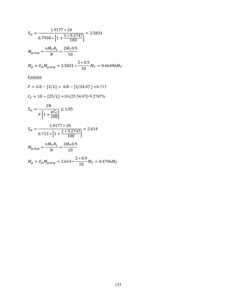
153
+Q = 1.9177 ∗ 106.7938 ∗ L1 + 1 ∗ 9.2747100 M = 2.5831
�U,>qU = /�xyz] = 2�x0.910
�U = +Q�U,>qU = 2.5831 ∗ 2 ∗ 0.910 �x = 0.46496�x Exterior
+ = 6.8 − [3 �⁄ ] = 6.8 − [3/34.47 ] =6.713
hC = 10 − [25 �⁄ ] =10-[25/34.47]=9.2747%
+Q = i]+ :1 + {hC100< ≥ 1.05
+Q = 1.9177 ∗ 106.713 ∗ L1 + 1 ∗ 9.2747100 M = 2.614
�U,>qU = /�xyz] = 2�x0.910
�U = +Q�U,>qU = 2.614 ∗ 2 ∗ 0.910 �x = 0.4706�x
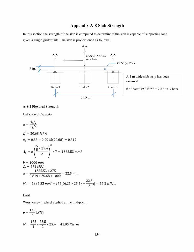
154
Appendix A-8 Slab Strength
In this section the strength of the slab is computed to determine if the slab is capable of supporting load
given a single girder fails. The slab is proportioned as follows.
A-8-1 Flexural Strength
Unfactored Capacity
^ = �5�,^��′V ��′ = 20.68 ��� ^� = 0.85 − 0.0015(20.68) = 0.819 �5 = � �58 ∗ 25.42 �
"∗ 7 = 1385.53 YY"
V = 1000 YY �, = 274 ���
^ = 1385.53 ∗ 2750.819 ∗ 20.68 ∗ 1000 = 22.5 YY
� = 1385.53 YY" ∗ 275[(6.25 ∗ 25.4) − 22.52 )] = 56.2 &]. Y
Load
Worst case= 1 wheel applied at the mid-point
� = 1752 (&]) � = 1754 ∗ 75.52 ∗ 25.4 = 41.95 &]. Y
CAN/CSA S6-06
Axle Load
Girder 2Girder 1 Girder 3
75.5 in.
7 in.
5/8” Ø @ 5” c.c.
A 1 m wide slab strip has been
assumed.
# of bars=39.37”/5” = 7.87 => 7 bars
155
Appendix B
Appendix B-1 Input File #1
Appendix B-2 Input File #2
Appendix B-3 Input File #3
Appendix B-4 Input File #4
Appendix B-5 Target Formation
Appendix B-6 Multi-Girder Code Input
Appendix B-7 Future Deterioration Sensitivity Study Results
Appendix B-8 Section Loss Results
Appendix B-9 Section Loss + Bond Deterioration Results

156
Appendix B-1 Input File #1
The following is a sample of the first input file required. The file describes the reinforcement as
line data from AutoCad.
Bar Start X-Coordinate End X-Coordinate Start Y Coordinate
Number of Re-Bars
157
Appendix B-2 Input File #2
The following is a sample of the second required input file. The file describes the spalling as
point data from AutoCad.
Point X-Coordinate Point Y-Coordinate

158
Appendix B-3 Input File #3
The third input file provides information regarding the bridge structure required for the strength
evaluation and appears as follows.

159

160
Appendix B-4 Input File #4
The last input file provides information regarding the load and load envelope as follows.

161
162
Appendix B-5 Target Formation
The following sample array is the formulation created within the program before the strength
evaluation begins.
2.0000 0 0 12.9900 254.00 213.010 1.2272 1.2272
6.0000 0 4.070 0 339.930 136.00 1.2272 1.2272
11.0000 0 0 95.8000 44.00 340.20 1.2272 1.2272
15.0000 0 0 37.6700 134.00 308.330 1.2272 1.2272
17.0000 0 4.070 0 333.930 46.00 1.2272 1.2272
22.0000 0 4.070 0 339.930 136.00 1.2272 1.2272
26.0000 0 0 8.3000 254.00 217.70 1.2272 1.2272
31.0000 1 128.94 224.200 5.060 121.80 0.1718 1.2272
35.0000 1 44.0 278.040 0 157.960 0 1.2272
Section in Spall? 1=Yes
ID of Bars present at section
Deteriorated Length (Right)
Deteriorated Length (Left)
Intact Length (Right)
Intact Length (Left)
Modified Area (Right)
Modified Area (Left)
Number of Re-Bars

163
Appendix B-6 Multi-Girder Code Input
When completing the full bridge analysis, the following combined input file should be created for each
girder instead of input file #1 an #2 for each.

164
0
500
1000
1500
2000
2500
3000
0 0.5 1
Moment (kip-in)
Distance x10-3 (in)
Scale-up Spalling (Girder 9-Moment)
0
40
80
120
160
200
0 0.5 1Shear (kip)
Distance x10-3 (in)
Scale-up Spalling (Girder 9-Simplified Shear)
0
40
80
120
160
200
0 0.5 1
Shear (kip)
Distance x10-3 (in)
Scale-up Spalling (Girder 9-General Shear)
0
0.005
0.01
0.015
0.02
0.025
0 0.5 1
R.I. (10^-3)
Distance x10-3 (in)
Scale up Spalling (Girder 9-RI Moment)
UnspalledCurrent SpallingScale by 1.25Scale by 1.5Scale by 2envelope
Appendix B-7 Future Deterioration Sensitivity Study Results

165
0
0.002
0.004
0.006
0.008
0.01
0.012
0 0.5 1
R.I. (10^-3)
Distance x10-3 (in)
Scale-up Spalling (Girder 9-RI Simplified Shear 1)
0
0.004
0.008
0.012
0.016
0 0.5 1
R.I. (10^-3)
Distance x10-3 (in)
Scale-up Spalling (Girder 9-RI General Shear)

166
Appendix B-8 Section Loss Results
Girder Intact Section Corrosion, �� Spalled Section Corrosion, �� 2 6% 15%
Distance, X (in)
Spalled Resistance
Flexural Envelope
Unspalled Resistance
Left
Support
Right
Support
Flexural Strength, (kip·ft)
Distance, X (in)
Shear Method #2
Flexural
Shear Method #1
Left
Support
Right
Support
Ratio of Spalled/U
nsp
alled R
esistance
167
Distance, X (in)
Spalled ResistanceShear Envelope
Unspalled Resistance
Left
Support
Right
Support
Shear Strength, (kip)
Positive Moment Region
Distance, X (in)
Min. Spalled ResistanceShear Envelope
Left
Support
Right
Support
Shear Strength, (kip)
Unspalled Resistance
Positive Moment Region

168
Distance, X (in)
Shear Method #1
Left
Support
Right
Support
Reliability Index
Flexure
Positive Moment Region
Shear Method #2
R.I.=3.5
169
Appendix B-9 Section Loss + Bond Deterioration Results
Girder Intact Section Corrosion, �� Spalled Section Corrosion, �� 2 6% 15%
Distance, X (in)
Spalled Resistance
Flexural Envelope
Unspalled Resistance
Left
Support
Right
Support
Flexural Strength, (kip·ft)
Distance, X (in)
Shear Method #2
Flexural
Shear Method #1
Left
Support
Right
Support
Ratio of Spalled/U
nsp
alled R
esistance
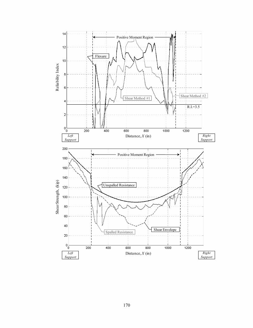
170
Distance, X (in)
Shear Method #1
Left
Support
Right
Support
Reliability Index
Flexure
Positive Moment Region
Shear Method #2
R.I.=3.5
Distance, X (in)
Spalled ResistanceShear Envelope
Unspalled Resistance
Left
Support
Right
Support
Shear Strength, (kip)
Positive Moment Region

171
Distance, X (in)
Min. Spalled ResistanceShear Envelope
Left
Support
Right
Support
Shear Strength, (kip)
Unspalled Resistance
Positive Moment Region
172
Appendix C
Appendix C-1 Test Specimen Detail
Appendix C-2 Test Specimen Design

Bar
Far
Near
X
150
153
G1
G2
Bar
Far
Near
X
140
147
G1
G2
Bar
Far
Near
X
150
149
G1
G2
X
X
X
1200
880 410
Beam #4
5mm Strain Gauges on Each Bar
180880
1200
Beam #3
5mm Strain Gauges on Each Bar
1200
180500
Beam #2
5mm Strain Gauges on Each Bar
1200100
8-3/16" Stirrups @ 200mm
100
2-1/4" x 1400mm Smooth
Bars
2-10M x 1240mm
Beam #1
Test Specimen Detail
DRAWING #:
DRAWN BY: DATE:JL Mar. 28 2011
6
Appendix C-1 Test Specimen Detail
173

G1
G2
Bar
Far
Near
X1
82
87
G3
G4
Far
Near
X2
95
97
G5
G6
Far
Near
G7
G8
Far
Near
X3 X4
78
80
93
96
G1
G2
X1 X2
X4X3X1 X2
180500
SikaTop 123 Plus Mortar PatchSikaWrap Hex 103C 850mm x 100mm
Longitudinal Fibers
Beam #8
380
Beam #5
2- 5mm Strain Gauges on Each Bar
12060
440
60
Beam #6
2- 5mm Strain Gauges on Each Bar
2- 5mm Strain Gauges on Each Bar
Test Specimen Detail
DRAWING #:
DRAWN BY: DATE:JL Sept. 2 2010
7
15090
180500
SikaTop 123 Plus Mortar Patch
Beam #7
3- 5mm Strain Gauges
Bar
Far
Near
X1
148
149
G3
G4
Far
Near
X2
143
144
G1
Bar
Far
X
140
G1
G2
Bar
Far
Far
X1
140
G3 Near
X2
140
295
174

180880
Sikacrete-08 SCC Patch
Beam #12
3- 5mm Strain Gauges on Near Bar
180500
SikaTop 123 Plus Mortar Patch
SikaWrap Hex 103C 400mm x 635mm
Vertical Fibers
Beam #10
180500
Sikacrete-08 SCC
Beam #11
3- 5mm Strain Gauges
180500
SikaTop 123 Plus Mortar PatchSikaWrap Hex 103C 850mm x 100mm
Longitudinal Fibers
SikaWrap Hex 103C 400mm x 635mm
Vertical Fibers
Beam #9
Test Specimen Detail
DRAWING #:
DRAWN BY: DATE:JL Sept. 2 2010
8
G1
G2
Bar
Far
Far
X1
140
G3 Far
X2 X3
415
293
G1
G2
Bar
Far
Far
X1
140
G3 Near
X2
145
300
175

176
Appendix C-2 Test Specimen Design
The following shows sample calculation for the design and evaluation of the lab specimens.
Only case (b) material strength calculations are shown here.
C-2-1 Development Length
�� = 1.0, �� = 1.0, �� = 1.0, � = 0.8
�� �� ��� � = 25 �� > �� = 11.3 �� �� �� ������� = 37.78 �� > 1.4�� = 15.82 ��
Minimum Stirrups provided
�" = 0.45 ������� #$
%#&′ ��
�" = 0.45 ∗ 0.8 ∗ 450√18.1 ∗ 11.3 = 430 ��
C-2-2 Moment Resistance (Unspalled)
)� = 0.85 − 0.0015#&′ = 0.85 − 0.0015 ∗ 18.1 = 0.8229
� = ,-#$)�#&′. = 200��� ∗ 450/0,
0.8229 ∗ 18.1/0, ∗ 100�� = 60.43 ��
/2 = ,-#$ 3� − �24 = 200��� ∗ 450/0, ∗ 5150 − 25 − 11.3
2 − 60.432 6 = 8.022 78. �
/9:; = <= , 0 = ∗>?@A
= = 8022B78. ��C ∗ ��DD99 = 26.74 78
Check Steel Strain
"E&
; = &D.DD�F
G = B119.35 − 73.43C ∗ 0.003573.43 = 0.00219 > 0.002 BH�� �� ��#��� �C
C-2-3 Shear Resistance (Unspalled)
�I = max M0.9�, 0.72ℎP = max Q0.9 ∗ 5150 − 25 − 11.32 6 , 0.72 ∗ 150R = 108��
,S = TB3/16" ∗ 25.4/2C� = 17.8��� ∗ 2 = 35.63���

177
Check Minimum shear reinforcement
,I9WX = 0.06%#&′.YZ#$
= 0.06 ∗ √18.1 /0, ∗ 100 ∗ 200��450 = 11.34 ��� < ,S B��C
Simplified Method
Assumed stirrups do not contribute to strength
�\] = 35 ∗ �\15 + ,_
= 35 ∗ 10815 + 9�� = 157.5��
` = 230B1000 + �\]C = 0.199, a = 35°
b& = c`%#&′ .Y�S = 1.0 ∗ 0.199 ∗ √18.1/0, ∗ 100�� ∗ 108�� = 9.144 78
b2 = b- + b&= 0+9.144 = 9.144 78 0 = b2 ∗ 2 = 18.28 78
General Method
Iterative spreadsheet created. b2 = 31.8 78
C-2-4 Moment Resistance (Spalled)
Spalled calculations shown for Beam #2 only.
,′ = ," d�W�"
e = 200��� d180430e = 83.72���
� = ,-#$)�#&′. = 83.72��� ∗ 450/0,
0.8229 ∗ 18.1/0, ∗ 100�� = 25.29 ��
/2 = ,-#$ 3� − �24 = 83.73��� ∗ 450/0, ∗ 5150 − 25 − 11.3
2 − 25.292 6 = 4.02 78. �
/9:; = <= , 0 = ∗>?@A
= = 4020B78. ��C ∗ ��DD99 = 13.478

178
C-2-5 Shear Resistance (Spalled)
Simplified Method
f;′ = ,-,-′
∗ f; = 20083.72 ∗ 0.00085 = 0.00203
` = 0.4B1 + 1500f;′C
1300B1000 + �\]C = 0.4
B1 + 1500 ∗ 0.00203C1300
B1000 + 157.5C = 0.1111
a = 29 + 7000 f;′ = 29 + 7000 ∗ 0.00203 = 43.21°
b& = c`%#&′ .Y�S = 1.0 ∗ 0.1111 ∗ √18.1 /0, ∗ 100�� ∗ 108�� = 5.105 78
b2 = b&= 5.10 K�
0 = b2 ∗ 2 = 10.2 78
General Method
Iterative spreadsheet created

179
Appendix D
Appendix D-1 Reliability Analysis Input File
180
Appendix D-1 Reliability Analysis Input File