Evaluating Subgrid-Scale Models for Large-EddySimulation of Turbulent Katabatic Flow

Bryan A. Burkholder, Evgeni Fedorovich, and Alan Shapiro

School of Meteorology, University of Oklahoma, 120 David L. Boren Blvd., Norman, OK,USA 73072 Bryan.A.Burkholder-1@ou.edu

Summary. The performance of commonly used subgrid-scale (SGS) models is evaluated forlarge-eddy simulation (LES) of turbulent katabatic flow. The very stable stratification andstrong low-level shear in this flow provide a stringent test for SGS models. Using an a poste-riori testing procedure, the SGS models’ performance in reproducing turbulence statistics andspectra in katabatic flow is investigated.

Key words: Large-Eddy Simulation, Subgrid-Scale Models, Katabatic Flow, A PosterioriTesting

1 Introduction

Over the past few decades, large-eddy simulation (LES) has become an invaluabletool for investigating the structure and characteristics of atmospheric boundary layerflows [1]. While encouraging results have been obtained from LES of neutrally strat-ified and unstable (convective) boundary layers, questions still remain concerningthe reliability of LES for reproducing stably-stratified turbulent boundary layers [2].Under stably-stratified conditions, the characteristic length scale of the small-scaleturbulent motions decrease, placing a larger burden on the subgrid-scale model em-ployed.

A plethora of subgrid/subfilter scale (SGS/SFS) models exist for wide varietyof applied problems in atmospheric dynamics. Reliable simulations have been per-formed in moderately stable boundary layers and have been successfully comparedto observational data [3]. However, no single SGS model appears significantly moreappropriate than another for a broad range of grid spacings. Typically, intercompar-isons test LES performance against direct numerical simulation (DNS) or measure-ment data. However, LES is run at much coarser resolutions than DNS and outputsfrom the two simulation techniques may not be directly comparable. Similarly, LESmay not incorporate all of the phenomena present in real flows when compared toobservational data. To fairly evaluate the performance of the SGS models, we em-ploy an a posteriori testing procedure [4][5]. To perform this type of procedure, the

M.V. Salvetti et al. (eds.), Quality and Reliability of Large-Eddy Simulations II,ERCOFTAC Series 16, DOI 10.1007/978-94-007-0231-8 14,© Springer Science+Business Media B.V. 2011

149

150 Bryan A. Burkholder, Evgeni Fedorovich, and Alan Shapiro

statistical behavior of the flow reproduced by LES is compared to filtered DNS datafor an identically forced flow.

We employ the a posteriori testing procedure in simulations of a shallow jet-likeflow developing along a cooled planar slope (katabatic flow). The earliest solutionsto this flow type can be traced back to studies by Prandtl [6], where the Boussinesqequations of motion were solved analytically for a laminar slope flow in a stably-stratified environment. The Prandtl solution is characterized by a strong near-surfacejet and weaker upslope flow aloft. It is no surprise that the turbulent counterpartof this flow is particularly difficult for LES, given the strong flow shear near thesurface accompanied by strong stable stratification. To futher complicate matters, nocomplete similarity theory has been developed yet for flows along sloping terrain[7]. These factors only compound the problems LES is known to have near boundingsurfaces, where the characteristic length scales of turbulent motions can be close tothe LES filter width [8]. Katabatic and anabatic (heated slope) flows have actuallybeen numerically investigated using LES with two different SGS closures [9][10],but the question regarding the optimal closure of LES for katabatic flows remainsunresolved.

2 Governing Equations and Closures

Following [6][11], we simulate a katabatic flow over a doubly-inifinite sloping sur-face which is inclined at a constant angle α with respect to the horizontal. In DNS,we solve the Boussinesq equations of motion and thermodynamic energy in rotatedcoordinates analagous to the ones adopted in [12][13] (Fig. 1). In the rotated coordi-nate system, x = x1 points in the downslope direction, y = x2 lies in the cross-slopedirection, and z = x3 is oriented normal to the slope.

In LES, we use the same rotated coordinates and solve the filtered Boussinesqequations of motion and thermodynamic energy,

∂ ui

∂ t+ u j

∂ ui

∂x j= b(−δi1sinα +δi3cosα)+ν

∂ ui

∂x j∂x j− ∂τi j

∂x j− 1

ρ∂ ¯p∂xi

, (1)

Fig. 1. Orientation of the coordinate system used (left) and a cross-sectional view of an ide-alized katabatic flow (right). The thin solid lines illustrate the stratification of the base-stateenvironment (θ∞), which is characterized by θ increasing linearly with height.

Evaluating SGS Models for LES of Turbulent Katabatic Flow 151

∂ b∂ t

+ u j∂ b∂x j

= −N2(−u1sinα + u3cosα)+κ∂ 2b

∂x j∂x j− ∂B j

∂x j, (2)

∂ ui

∂xi= 0, (3)

withτi j = uiu j − uiu j, (4)

B j = ˜bu j − bu j, (5)

¯p = p+23

E, (6)

where ˜(...) indicates a quantity filtered using a top-hat filter, N is the Brunt-Vaisalafrequency (which is set to a constant value), τi j is the subgrid momentum flux (neg-ative of the subgrid stress tensor), B j is the subgrid buoyancy flux, p is the filteredpressure, ¯p is the modified pressure, and E is the subgrid/subfilter turbulence ki-netic energy (TKE). The top-hat filter width, Δ , is taken to be equal to the LES gridspacing. Buoyancy is defined as

b = gθ −θ∞

θr, (7)

where g is gravitational acceleration, θ is potential temperature, θr is a constantreference potential temperature, and θ∞ is the environmental potential temperaturewhich is taken to vary linearly with height. To close the system of filtered equations,τi j and B j must be parameterized in terms of the resolved flow fields.

One of the earliest SGS models used for meteorological applications was theSmagorinsky model [14], which employs the assumption of a balance between shearproduction and the dissipation of subgrid TKE. As a result, the SGS stress tensor istaken proportional to the resolved strain rate tensor:

νT = [CSΔ ]2S, (8)

τi j = Eδi j −2νT Si j, (9)

where S =√

2Si jSi j and CS is known as the Smagorinsky coefficient. Using a sharpcutoff filter in the inertial subrange and assuming the Kolmogorov scaling, CS wasfound to be roughly 0.17 [15]. The value of CS has also been found to vary signifi-cantly depending on the type of flow simulated [8]. A value around 0.2 is commonlyused in atmospheric contexts [1]. While reasonable results can be attained using theSmagorinsky model, the underlying assumption that the SGS stress tensor is pro-portional to the strain rate is a critical one, and may not necessarily be valid in allapplications. The model is also known to be overly dissipative, especially near thesurface. Despite its inherent disadvantages, this SGS model is still implemented as abaseline model in LES of many atmospheric flows because of its simplicity.

Deardorff [16] considered another form of the subgrid TKE balance by includingbuoyancy effects and subgrid energy transport. The subgrid TKE is then calculated

152 Bryan A. Burkholder, Evgeni Fedorovich, and Alan Shapiro

as a prognostic variable from a simplified version of its governing equation [17] andis used to parameterize the eddy viscosity locally through

νT = CDl√

E, (10)

κT = (1+2lΔ

)νT , (11)

l =

⎧

⎪

⎪

⎪

⎪

⎨

⎪

⎪

⎪

⎪

⎩

Δ∂ b

∂ z≤ 0,

min[Δ ,0.5√

E/(∂ b/∂ z)]∂ b

∂ z> 0.

(12)

The adopted dependence of the mixing length on the stratification (Eq. 12) is usedto decrease the turbulent length scale when stable stratification is encountered. Theparameter CD was set to 0.12 in [16]. Even though [16] used this l scaling factorwithin stratocumulus cloud layers, it is currently implemented in many SGS modelsthat are used in general atmospheric applications.

Both considered formulations, however, do not account for the backscatter ofenergy from small scales to larger scales, which may be important in parameteriz-ing the SGS motions [18][19][20]. To counteract the overly dissipative nature of theschemes proposed by [14] and [16], some form of non-linear or stochastic backscat-tering mechanism has been suggested for simulations of stable boundary layers in[1][21]. The original stochastic backscattering model of [19] was computationallyexhaustive and did not match Monin-Obukhov similarity near the surface. Sullivan[22] argued that this backscatter behavior could be accounted for by using adequategrid resolution and less dissipative SGS closures. A two-part model was proposed, inwhich the near-surface region was controlled by the mean shear and the region awayfrom the surface followed the closure [16]:

τi j = −2νT′γ Si j −2νT 〈Si j〉+Eδi j, (13)

where 〈...〉 represents averaging in homogeneous directions (slope-parallel planes inthe case of laterally homogeneous flow), νT

′ is the fluctuating field-eddy viscosity,νT is the mean-field eddy viscosity, and γ is the isotropy factor:

γ =S′

〈S〉+ S′, (14)

where S′ is the fluctuating strain rate. The calculation of the isotropy factor allows asmooth transition from an ensemble-average approach near the ground to the base-line subgrid TKE model of [16] in the main portion of the flow. The SGS buoyancyflux was found to be important in moderately stable conditions and was later includedin the two-part formulation [23].

Another method to modify the classic Smagorinsky model is to dynamically cal-culate CS. This approach employs a larger filter width, for example, Δ = 2Δ , and

Evaluating SGS Models for LES of Turbulent Katabatic Flow 153

then uses the filtered fields to calculate the Smagorinsky coefficient using the Ger-mano identity [24]. Rather than specifying the coefficient, the SGS model essentiallycalculates its optimal value from the resolved fields. To statistically minimize the er-ror and find this optimal value, averaging over some homogeneous direction mustbe applied [25]. Preferably, this averaging should be performed over Lagrangianpaths or over the nearest grid cell neighbors in homogeneous directions [26]. A third,even larger filter width, Δ = 2 Δ = 4Δ , can be introduced to make the model scale-dependent using a power-law relation between filter widths [27][28]. Even thoughthe dynamic versions of the original Smagorinsky type-closure can essentially adjustthe characteristic length scale of the subgrid-scale motions, it cannot reproduce thebackscattering and anisotropy necessary to correctly simulate the turbulence in thestable boundary layer [21].

3 Model setup and flow characteristics

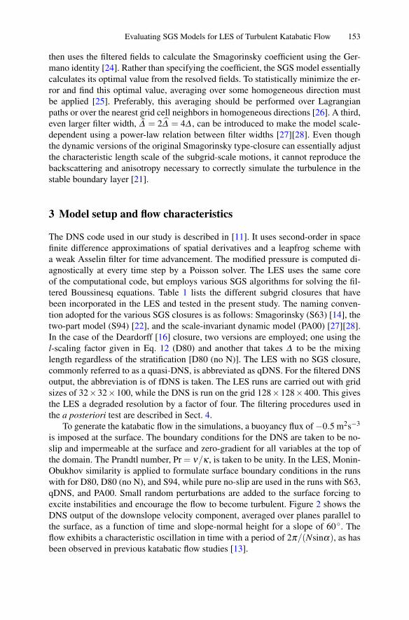
The DNS code used in our study is described in [11]. It uses second-order in spacefinite difference approximations of spatial derivatives and a leapfrog scheme witha weak Asselin filter for time advancement. The modified pressure is computed di-agnostically at every time step by a Poisson solver. The LES uses the same coreof the computational code, but employs various SGS algorithms for solving the fil-tered Boussinesq equations. Table 1 lists the different subgrid closures that havebeen incorporated in the LES and tested in the present study. The naming conven-tion adopted for the various SGS closures is as follows: Smagorinsky (S63) [14], thetwo-part model (S94) [22], and the scale-invariant dynamic model (PA00) [27][28].In the case of the Deardorff [16] closure, two versions are employed; one using thel-scaling factor given in Eq. 12 (D80) and another that takes Δ to be the mixinglength regardless of the stratification [D80 (no N)]. The LES with no SGS closure,commonly referred to as a quasi-DNS, is abbreviated as qDNS. For the filtered DNSoutput, the abbreviation is of fDNS is taken. The LES runs are carried out with gridsizes of 32×32×100, while the DNS is run on the grid 128×128×400. This givesthe LES a degraded resolution by a factor of four. The filtering procedures used inthe a posteriori test are described in Sect. 4.

To generate the katabatic flow in the simulations, a buoyancy flux of −0.5 m2s−3

is imposed at the surface. The boundary conditions for the DNS are taken to be no-slip and impermeable at the surface and zero-gradient for all variables at the top ofthe domain. The Prandtl number, Pr = ν/κ , is taken to be unity. In the LES, Monin-Obukhov similarity is applied to formulate surface boundary conditions in the runswith for D80, D80 (no N), and S94, while pure no-slip are used in the runs with S63,qDNS, and PA00. Small random perturbations are added to the surface forcing toexcite instabilities and encourage the flow to become turbulent. Figure 2 shows theDNS output of the downslope velocity component, averaged over planes parallel tothe surface, as a function of time and slope-normal height for a slope of 60◦. Theflow exhibits a characteristic oscillation in time with a period of 2π/(Nsinα), as hasbeen observed in previous katabatic flow studies [13].

154 Bryan A. Burkholder, Evgeni Fedorovich, and Alan Shapiro

Table 1. List of abbreviations for different DNS/LES runs. The asterisk indicates that themixing length scaling factor in Eq. 12 was not used.

Abbreviation Type (citation)

DNS DNSfDNS DNS (filtered to LES grid)qDNS LES (no closure)S63 LES [14]D80 LES [16]D80 (no N) LES [16]*S94 LES [22]PA00 LES [27][28]

Fig. 2. DNS results of downslope velocity in a katabatic flow along a 60◦ sloping surface. Thebold contour demarcates the transition between positive and negative values of the along-slopecomponent of velocity.

The two parameters that completely determine the flow in this case are α and|F0|ν−1N−2, where F0 is the buoyancy flux imposed at the surface [13][29]. Thecharacteristic length, velocity, and buoyancy scales of the flow in the present studyare given, respectively, by

ls =√

|F0|N−3, us =√

|F0|N−1, bs =√

|F0|N. (15)

Evaluating SGS Models for LES of Turbulent Katabatic Flow 155

Taking the governing parameters for the flow to be F0 = −0.5 m2s−3, N =1 s−1,and ν = 10−4 m2s−1, we obtain |F0|ν−1N−2 = 5000 with characteristic scalesls = 0.71 m, us = 0.71 ms−1, and bs = 0.71 ms−2. Alternatively, we can chooseother parameter values provided that |F0|/νN2 = 5000, which would result in ex-actly the same scaled flow solutions. For example, selecting values commonlyfound in atmospheric applications such as N = 10−2 s−1, ν = 0.1 m2s−1, and F0 =−0.05 m2s−3, our characteristic scales become ls2 = 220 m, us2 = 2.2 ms−1, andbs2 = 0.022 ms−2. Throughout the paper, we use the first set of scales to presentresults in a dimensional form.

4 A Posteriori Testing

A posteriori testing is commonly used to compare LES flow statistics to the thoseprovided by a DNS of an identically forced flow. Since DNS typically has a higherresolution than LES, the DNS fields must be filtered down to the LES grid. To do this,a top-hat filter that has the width of the LES filter is applied. The effect of filteringthe DNS output to the LES grid is shown in the top two panels of Fig. 3. It is seenthat some of the smaller-scale features are lost through the filtering operation, butthe overall visual characteristics of the flow do not change significantly. Since thefiltered DNS output would be the best field LES could ever reproduce at a degradedresolution, it is taken as a reference flow field.

Normally, differences found in comparing an LES output to the filtered DNSresults could potentially originate from different SGS models, numerical discretiza-tions in space, time advancement schemes, or resolutions [4]. In our case, since eachLES run is completed using identical numerical schemes, virtually all of the differ-ences are expected to originate from the SGS models. In Fig. 3, we can see that nearthe surface, all tested SGS closures tend to organize the near-surface flow into large-scale structures which are absent in the filtered DNS field. This could be due to theover-dissipative nature found in some of the schemes, but also may be an effect ofthe insufficient grid resolution near the surface. The level depicted in Fig. 3 is onlythe 8th point above the surface for LES, while it is the 32nd point above the groundfor DNS. It is likely the problems that LES has near bounding surfaces in moder-ate to high Reynolds number flows are still observed at this level above the lowerboundary. The dynamic closure and the qDNS share the most visual similarities withthe filtered DNS output. This may be due to the the schemes being under-dissipative,which is briefly discussed below.

The one-dimensional velocity spectra shown in Fig. 4 demonstrate that most ofthe SGS closures produce the desired general spectral characteristics. The velocityspectra are calculated according to [30] and are averaged in time over at least six os-cillations (see Fig. 2). This smooths the spectra making them easier to interpret. Nearthe surface, LES spectra obtained with S63 and S94 schemes are almost identical tothe fDNS spectrum. The one spectrum that does not exhibit reasonable behavior isfrom the qDNS, which follows the -5/3 line at exceedingly high wavenumbers. In theplot with their dissipation spectra, D11(k) = 2νk2E11(k), turbulence in the qDNS is

156 Bryan A. Burkholder, Evgeni Fedorovich, and Alan Shapiro

Fig. 3. Horizontal contour plot of downslope velocity on a plane parallel to the sloping surface.Each panel starting at the top left and going to the right and down, shows a) the output fromDNS, b) the DNS output filtered to the LES grid, c) qDNS, d) S63, e) D80, f) D80 (no N), g)S94, and h) PA00. In each plot, the LES grid spacing is illustrated by the thin black lines.

Evaluating SGS Models for LES of Turbulent Katabatic Flow 157

found to be dissipating improperly. Most of the energy in this spectrum dissipates atwavenumbers very close to the Kolmogorov scale. All of the SGS closure schemesshow reasonable spectral dissipation properties, as most of the dissipation occurs atwavenumbers much smaller than the Kolmogorov scale. The discrepancies betweenthe different SGS closures become smaller with height, as the LES is able to resolvethe motions at these levels. However, the D80 TKE-based schemes appear to beslightly over-dissipative, even at substantial distances from the slope. For katabaticflows, the S63 scheme performance appears to be reasonable, at least once turbu-lence has already developed. As has been previously reported, the dynamic model isunder-dissipative close to the surface [27], but performs reasonably well in regionsaway from the surface.

Fig. 4. Time-averaged normalized u1 spectra at DNS level 32 (LES level 8) (top, left) and theirrespective dissipation spectra (top,right). The same is shown at level 160 in the bottom twopanels.

From Fig. 5, we conclude that LES is roughly capable of reproducing the correctflow in terms of mean velocity and buoyancy which are obtained by averaging overplanes parallel to the surface and over six oscillations in time. Not surprisingly, theLES performance is worse for higher order statistics, as is seen for the total turbulentfluxes and the variances, especially near the surface. When comparing the ratios ofthe total contribution of each velocity variance to the to total velocity componentvariance, we can see that the fDNS exhibits 〈˜u′1u′1〉 that is about 3 times larger than

〈˜u′3u′3〉, where the angle brackets here denote the combined spatial (over planes paral-

158 Bryan A. Burkholder, Evgeni Fedorovich, and Alan Shapiro

Fig. 5. Temporal and planar-averaged profiles (〈...〉) of a) 〈u1〉, b) 〈b〉, c) 〈 ˜u′1u′1〉, d) 〈 ˜u′3u′3〉,e) 〈 ˜u′1u′3〉, and f) 〈˜u′3b′〉 as a function of z.

lel to the slope) and temporal (over several flow oscillations) averaging. Meanwhile,LES tends to have larger ratios of variance components, with 〈˜u′1u′1〉 being about a

factor of 4.5 - 10 times larger than 〈˜u′3u′3〉. Near the surface, the TKE-based SGSclosures generate a pronounced spike in vertical velocity variance. An analysis ofthe subgrid TKE budget (not shown) reveals that the near-surface shear productionassociated with the katabatic jet is responsible for the spike. Some of the SGS modelstested (especially the S63 model) also tend to over-predict the slightly negative verti-

Evaluating SGS Models for LES of Turbulent Katabatic Flow 159

cal momentum flux near the surface that is observed in the DNS output. Interestingly,for the buoyancy related fields, the LES with no SGS model (qDNS) outperformedsome LES with SGS formulations. It should be noted that the correction of the Sul-livan [22] scheme for scalars implemented in [23] was not tested.

5 Conclusions

Overall, the performance of the basic SGS closures employed by LES for atmo-spheric applications is acceptable for mean fields, but degrades noticeably whenit comes to higher-order statistics (particularly buoyancy fluxes). Near the ground,where the SGS contributions compose the largest portion of the total fluxes and vari-ances, the different closures produce highly variable results. The over-production ofsubgrid TKE by the shear close to the surface causes errors in the models based on[16] and especially affect the vertical velocity variance. Also, many of the testedschemes drastically overestimate the negative momentum flux near the ground. Amajority of the tested schemes are able to capture the anisotropy of the flow in thealong-slope direction, though this feature of the flow is also slightly overestimatedby the LES.

With respect to velocity spectra, the [22] and [14] schemes perform the best nearthe ground, while the dynamic and two-part models perform better in turbulent re-gions of the flow away from the surface. Even though the solution produced by theqDNS remains stable, it exhibits a build-up of energy as well as unrealistic dissipa-tion at high wavelengths. The schemes based on [16] are found to be over-dissipative,and flow statistics slightly improved when the mixing length stratification adjustmentafter [16] is not used.

The extension of testing toward other SGS models will constitute the scope offuture studies. Updating the time advancement schemes in both DNS and LES isalso planned. The influence of the varying slope angle on the performance of theSGS models in LES of katabatic flows should be studied as well.

References

1. Mason PJ (1994) Bound-Layer Meteor 120:1–262. Mahrt L (1998) Theoret Comput Fluid Dyn 11:263–2793. Beare RJ, MacVean MK, Holtslag AAM, Cuxart J, Esau I, Golaz JC, Jimenez MA,

Khairoutdinov M, Kosovic B, Lewellen D, Lund TS, Lundquist JK, McCabe A,Moene AF, Noh Y, Raasch S, and Sullivan P (2006) Bound-Layer Meteor 118:247–272

4. Geurts B (2004) Elements of direct and large-eddy simulation. R. T. Edwards, Inc.,Philadelphia, PA

5. Vreman B, Geurts B, and Kuerten H (1997) J Fluid Mech 339:357–3906. Prandtl L (1942) Fuhrer durch die Stromungslehre. Vieweg & Sohn, Braunschweig7. Denby B (1999) Bound-Layer Meteor 92:67–1008. Pope SB (2000) Turbulent flows. Cambridge University Press, Cambridge9. Schumann U (1990) Quart J Roy Meteor Soc 116:637–670

160 Bryan A. Burkholder, Evgeni Fedorovich, and Alan Shapiro

10. Skyllingstad ED (2003) Bound-Layer Meteor 106:217–24311. Shapiro A and Fedorovich E (2004) Int J Heat and Mass Transfer 47:4911–492712. Burkholder BA, Shapiro A, Fedorovich E (2009) Acta Geophysica (in press, DOI:

10.2478/s11600-009-0025-6)13. Fedorovich E and Shapiro A (2009) Acta Geophysica (in press, DOI: 10.2478/s11600-

009-0027-4)14. Smagorinsky J (1963) Mon Wea Rev 91:99–16415. Lilly DK (1967) Proc IBM Sci Computing Symp Environmental Sci 320-1951:195–21016. Deardorff JW (1980) Bound-Layer Meteor 18:495–52717. Piomelli U and Chasnov JR (1996) Large-eddy simulations: theory and applications. In:

Henningson D, Hallback, Alfreddson H, and Johansson A (eds) Transition and turbulencemodelling. Kluwer Academic Publishers, Dordrecht

18. Leslie DC and Quarini GL (1979) J Fluid Mech 91:65–9119. Mason PJ and Thomson DJ (1992) J Fluid Mech 242:51–7820. Brown AR, Derbyshire SH, Mason PJ (1994) Quart J Roy Meteorol Soc 120:1485–151221. Kosovic B (1997) J Fluid Mech 336:151–18222. Sullivan PP, McWilliams JC, Moeng C (1994) Bound-Layer Meteor 71:247–27623. Saiki EM, Moeng C, and Sullivan PP (2000) Bound-Layer Meteor 95:1–3024. Germano M, Piomelli U, Moin P, Cabot WH (1991) Phys Fluids A 7:1760–177125. Lilly DK (1992) Phys Fluids A 4:633–63526. Stoll R and Porte-Agel F (2008) Bound-Layer Meteor 126:1–2827. Porte-Agel F, Meneveau C, Parlange MB (2000) J Fluid Mech 415:261–28428. Porte-Agel (2004) Bound-Layer Meteor 112:81–10529. Fedorovich E and Shapiro A (2009) J Fluid Mech (in press)30. Kaiser R and Fedorovich E (1998) J Atmo Sci 55:580–594