Evaluating Static Worst-Case Execution-Time Analysis for a Commercial Real-Time Operating System

Daniel Sandell Master’s thesis

D-level, 20 credits Dept. of Computer Science

Mälardalen University

Supervisor: Andreas Ermedahl Examiners: Björn Lisper, Jan Gustafsson

July 22, 2004

Abstract The worst case execution time (WCET) of a task is a key component in the design and development of hard real-time systems. Malfunctional real-time systems could cause an aeroplane to crash or the anti-lock braking system in a car to stop working. Static WCET analysis is a method to derive WCET estimates of programs. Such analysis obtains a WCET estimate without executing the program, instead relying on models of possible program executions and models of the hardware. In this thesis WCET estimates have been derived on an industrial real-time operating system code with a commercial state-of-the art WCET analysis tool. The goal was to investigate if WCET analysis tools are suited for this type of code. The analyses have been performed on selected system calls and on regions where interrupts are disabled. Our results indicate that static WCET analysis is a feasible method for deriving WCET estimates for real-time operating system code, with more or less intervention by the user. For all analysed code parts of the real-time operating system we were able to obtain WCET estimates. Our results show that the WCET of system calls are not always fixed but could depend on the current state of the operating system. These things are by nature hard to derive statically, and often require much manual intervention and detailed system knowledge. The regions where interrupts are disabled are easier to analyse automatically, since they are usually short and have simple code structures.

1

Acknowledgments I would like to thank my supervisor Andreas Ermedahl for all support and help during this thesis, Jan Lindblad at Enea Embedded Technology that helped me with the OSE operating system code, Martin Sicks at AbsInt that answered my questions about the aiT WCET tool. I would also like to thank Jan Gustafsson, Christer Sandberg and Björn Lisper from the WCET-team at Mälardalen University for their support.*

* This thesis was performed within the Advanced Software Technology (ASTEC) competence centre (www.astec.uu.se), supported by VINNOVA.

2

Contents

1. Introduction 4 2. Overview of the work 5 3. Uses of WCET analysis 6 3.1 Embedded systems 6 3.2 Real-time systems 6 3.3 The need of a safe WCET estimate result 7 3.4 Obtaining worst case execution time estimates 8

4. Overview of static WCET analysis and related work 9 4.1 Flow analysis 10 4.2 Low-level analysis 16 4.3 Calculation 20 4.4 WCET analysis tools 22 4.5 Related work 24 5. Industrial code and analysis environment 26 5.1 Industrial code 26 5.2 The aiT WCET analysis tool 28 5.3 ARM 34 5.4 Object code 39 6. Experiments 41 6.1 Analysis of system calls 41 6.2 Analysis of disable interrupt regions 43 6.3 Testing of a hardware model 45 6.4 How optimisations affects the WCET results 47

7. Conclusions 51 8. Future Work 52 Bibliography 53

Appendix 55

3

1. Introduction In real-time systems it is very important to know the worst case execution time (WCET) of a task to guarantee that a task will finish its execution before its deadline. A task missing its deadline in a hard real-time system can have catastrophically consequences. Examples of hard real-time systems are medical equipments, flight control systems and anti-lock braking systems in a car. Today, the most common way to derive WCET estimates is measurements. That is, run the programs with different input values and system states, trying to find the combination that gives the WCET. However, it is in practice impossible to run most programs with all possible inputs. Therefore, measurements cannot guarantee that the actual WCET result has been found. Another method to obtain WCET estimates of a program is static WCET analysis. Such analysis obtains a WCET estimate without executing the program relying on models of possible program executions and models of the hardware. Today, there exists both commercial and research WCET analysis tools. However, such analyses are still not commonly used in the industry and not so many analyses have been performed by researchers on complex real-world programs. The purpose with this thesis was to test how static WCET analysis can be used on real operating system code. The commercial WCET analysis tool aiT was used in the analyses. The analyses were performed on industrial code from the OSE operating system. OSE is one of the world leading operating systems for embedded systems. It is a quite large system, modularly built to allow easy porting on different hardware platforms. The analyses of the operating system code were performed on some selected system calls and disable interrupt regions. To get an estimation of the quality of the analyses a comparison was performed. Estimates produced by the WCET analysis tool were compared to timing estimates produced by a clock cycle accurate hardware simulator developed by the processor manufacture [2]. Our result shows that the WCET of system calls are not always fixed but could depend on the current state of the operating system. These things are by nature hard to derive statically, and therefore require much manual intervention and detailed system knowledge. However, the regions where interrupts are disabled are usually short and are easier to analyse automatically. In general the analyses show that it is possible to use a WCET analysis tool with more or less intervention by the user. Thesis outline. The thesis is organised as follows: Section 2 presents an overview of the analyses performed. Section 3 gives a more detailed description of the uses of WCET analysis. An overview of static WCET analysis and related work is presented in Section 4. Section 5 presents the OSE code that has been used in most of the analyses and also the analysis environment. The result of the experiments is given in Section 6. In Section 7 our conclusions are presented and suggestions to future work are given in Section 8.

4

2. Overview of the work In this thesis static WCET analysis is used to estimate the longest execution times of programs or part of programs. Static WCET analysis is a method to analyse a program without executing the program, and to give safe WCET estimate results. The purpose with this thesis was to see if a WCET analysis tool could be used to derive WCET estimates on code from the OSE operating system. Another reason was to investigate what has to be improved in current WCET analysis tools to make WCET analysis tools more applicable to demands of the industry. The work can be divided into two parts, WCET analyses and estimation of a hardware model. A simplified structure over the work is shown in Figure 2.1.

Figure 2.1: Simplified structure of the analyses. Most of the WCET analyses have been performed on code from the OSE operating system including system calls and disable interrupt regions. Also some analyses have been performed on benchmarks code with different levels of optimisations, to see how much manual work that have to be redone when optimising a program. The WCET analysis tool used in this thesis performs the analysis directly on the executable code. To obtain the executable code, the source files of a program have to be compiled with a compiler. From the WCET analysis tool, estimated WCET results were produced, analysed on the ARM7TDMI processor. To show that the results produced by the WCET analysis tool are safe and to get an estimation of the quality. Timing estimates derived using a hardware simulator were compared to the results obtained by the WCET analysis tool. The analysed OSE operating system code contains of both code written in C and assembler. While all benchmarks only contains code written in C.

5

3. Uses of WCET analysis In this section we will try to explain the uses of WCET analysis, including background information of embedded systems and real-time systems. In this section we will also look at methods to derive WCET estimates. 3.1 Embedded systems An embedded system is a system that is embedded as a component of a product. It is a computer that is used to achieve some specific goal, not a goal in itself. The design of an embedded processor is often less complex than a desktop processor, because an embedded processor is often specialised to perform a specific task. Therefore an embedded processor is often much cheaper than a desktop processor. There are several things that influence the choice of embedded processor e.g., cost, size, energy consumption and the type of task to be performed. Today there are many different manufactures of embedded processors and it is no specific architecture or manufacture that clearly dominates the market. Examples of manufacturers and architectures are ARM, PowerPC and NEC.

Figure 3.1: Communication networks and computers in Volvo S80 [34] An example of where embedded systems exist is in a car. Figure 3.1 illustrates the communication network in Volvo S80. Two CAN (Controller Area Network) communication systems are used for communication between microprocessors. The microprocessors are placed on strategic places in the network and each microprocessor is used to perform a specific function [34]. 3.2 Real-time systems Most embedded systems are also real-time systems. A real-time system is a system that reacts on external events and performs functions based on these events. A common mistake is to think that a real-time system is the same as a system that tries to execute as fast as possible, but in a real-time system the correctness of the result depends on when the result is produced [33]. A real-time system can be time triggered, event triggered or a combination of both. Strictly time triggered systems handles external events at prescheduled time. This type of systems often repeats a function within a specified period of time. In a strictly event triggered system it is instead external events that decides when a task should execute.

6

Real-time systems can be classified as hard, soft or a combination of both. A hard real-time system is a system where the costs of not fulfil either the temporal or the functional constraints is very high. A task missing its deadline in a hard real-time system could have catastrophic consequences. Hard real-time systems are often time triggered. Examples of hard real-time systems are monitoring system in a nuclear power plant, flight control system and anti-lock braking controller. For example, when the driver of the car presses the brake-pedal, the anti-lock braking controller activates the brake with appropriate frequency that depends on car speed and road surface. To insure the safety of the driver, both the brake activation and the time at which the result is produced are important [9]. A soft real-time system is a system where meeting of deadlines are desirable, but where a few deadlines misses could be tolerated. Examples of soft real-time systems are: multimedia products, music technology and telephone systems. For example, a telephone system is an event triggered system, that reacts when a subscriber dial a number. This system will work well in the normal case, but not in extraordinary cases when many subscribers try to use the system at the same time. Then some subscribers will not be able to use the system [34]. 3.3 The need of a safe WCET estimate result In the development of real-time systems, different schedule analyses are often used to be able to predict the behaviour of the system in advance. These analyses assume that the worst execution time of each individual task is known. An illustrative example of a schedule of three tasks is given in Figure 3.2.

Figure 3.2: Example of tasks that can be scheduled This example consists of three tasks, A, B and C. Each task is ready to execute at time unit 0, and each task has a deadline constraint of 10 time units meaning that each task has to finish its execution 10 time units after it was ready to execute. The execution times of task A, B and C are 6, 3 and 1 time units respectively. Task A starts to execute, followed by task B, and finally task C executes. In this example all tasks finished executing before their deadlines and consequently the system is schedulable. Figure 3.3 gives the same example, but with the execution time of task A being 7 time units instead of 6.

7

Figure 3.3: Example of tasks that cannot be scheduled Task A and task B will be able to finish their execution before its deadline, but task C is missing its deadline. Therefore it is not possible to schedule these tasks. This shows that when designing real-time systems it is important to not underestimate the actual WCET of a task, otherwise a task could miss its deadline and maybe cause catastrophic consequences. 3.4 Obtaining worst case execution time estimates The most common method in the industry to obtain WCET estimates is by measuring a program with different input data. Two common methods are partition testing and structural testing. In partition testing the input domain is divided into sub domains, and selects test data for each sub domain. In structural testing the programmer examines the source code of the program. The coverage of the test data is based on the percentage of the program’s statements executed [9]. Execution times can be obtained in several ways, for instance with an oscilloscope, logic analyser or with a hardware simulator. One disadvantage with measuring is that it cannot guarantee that the actual WCET result has been found. To measure all the execution times of a program with all possible inputs is practice impossible, for instance if the input values to the program foo(x,y,z) are 16-bit integers will lead to 248 possible executions. To measure all possible executions will take 9000 years if each measure takes 1 ms. Static WCET analysis is an alternative method to obtain WCET estimates. The advantage with this method is that if safe assumptions are made about the hardware and about the dynamical program behaviour then it can guarantee that no underestimations occur. In the following section, static WCET analysis will be described more in detail.

8

4. Overview of static WCET analysis and related work The method studied in this report is static WCET analysis. The analysis relies on models of the program and the timing behaviour. A static WCET analysis must be both safe and tight i.e., if an underestimating occur then it is possible that a task can miss its deadline and to be useful the WCET estimate must be as close as possible to the actual WCET. In this section we will look at the different phases of a static WCET analysis. We will also look at some related work. Figure 4.1 shows the structure of WCET analysis.

Figure 4.1: The structure of WCET analysis [18]. Static WCET analysis is traditionally divided into three main phases:

• Flow analysis: Is used to determine the dynamic behaviour of a program e.g., how many times a loop iterates, dependencies between if-statements and what functions that gets called.

• Low-level analysis: Is performed on the object code of a program to obtain the actual

timing behaviour. The analysis can be divided into a global and local low-level analysis. The global analysis is used to analyse effects over the entire program to be able to get a safe and tight result e.g., for effects of caching. The local analysis is used to analyse effects of a single instruction and its neighbour instructions that can be handled locally e.g., effects of pipelining. For some complex processors it can be difficult to make this division.

• Calculation: The result from the flow and low-level analysis phases are combined to

calculate the final WCET estimate. There are three basic calculation methods, tree-based, path-based and IPET (Implicit Path Enumeration Technique). The different calculation methods are described more in detail in Section 4.3.

9

4.1 Flow analysis Flow analysis is used to determine possible and impossible program flows, for instance which function is called, how many times a loop iterates and dependencies between if-statements. To analyse all properties of a program automatically is impossible due to it is equivalent to the well-known Halting problem, stating that it is impossible to construct a program that is able to determine, for any other program, if it will halt or not. This means that safe approximations sometimes have to be used and that not all programs can be analysed. The approximations need to be safe, so that no sub path that could be in the WCET path is removed. The approximations needs also to be as tight as possible i.e., as few paths as possible should be included in the estimated WCET result.

Figure 4.2: Components of flow analysis [16]. Flow analysis can be performed on the source code, object code or intermediate code level and it can be divided into three sub-stages as illustrated in Figure 4.2.

1. Flow extraction: In this stage the code is analysed, it could be done manually or automatically. 2. Flow representation: A representation of the extracted flow information comes in form of a graph, syntax-tree or program code, to make it both readable for humans and also easy to be processed by tools. 3. Calculation conversion: The flow representation is converted so it can be used in the calculation.

4.1.1 Flow extraction In the flow extraction stage the code is analysed manually or automatically with help of tools [1, 6,18]. Because manual analysis is very time consuming and also error prone, it is preferred to analyse the code automatically if possible. One of way to analyse the behaviour of a program is by using abstract interpretation. Abstract interpretation [11] is a method to analyse runtime behaviour of a program with all possible input values to the program without executing the real program. Instead of using real values, variables have instead abstract values e.g., a variable can sometimes have several values instead of one. This can lead to overestimations, but done correctly it could be guaranteed that the results are safe. In [21] Gustafsson uses semantic analysis based on abstract interpretation to automatically find information about infeasible paths and maximum number of iterations in loops. The method consists of three parts:

10

• Program instrumentation: The original program is modified to be able to obtain

information about the execution history. • Path analysis: Calculation of iteration count and identifications of paths are performed

while doing abstract interpretation of the program.

• Merging: To avoid an exponential growth of path to be analysed, the results are merged at end of loop bodies and after termination of loops.

An example of code that can be analysed is shown in Figure 4.3 and the resulting analysis structure is shown in Figure 4.4. l1 is a loop label and e1 to e4 are edge labels. Each variable in the analysis can have a set of values and the set of values is represented by an interval. The initial value of x is assumed to be in the interval [0..3], where x is an integer. A loop iteration is indicated with a #, and an infeasible path is indicated with a dashed line.

Figure 4.3: Code example [21].

Figure 4.4: Analysis structure [21]. The loop cannot terminate in the interval [0..3], so it continues with the first iteration. In the first if-statement both paths are feasible. When entering e1, x is must be in the interval [0..2] and resulting in the new interval [0..4] after execution x=x*2. e2 is analysed in a similar way, x entering with interval [3..3] and it will result in the new interval [4..4].

11

In the second if-statement x can have a value from two different intervals [0..4] and [4...4]. The first interval will result in two feasible paths, but because the second interval only consists of the value 4, it will result in one feasible and one infeasible path i.e., the infeasible path means that a path including both e2 and e3 is not feasible during the first iteration. Now the analysis of the first iteration is finished. The value of x can be in three different intervals [3..3], [1..5] and in [5..5]. To reduce the complexity of the calculation, the intervals are merged and it results in a union of all variable values i.e., the new interval [1..5]. After that the interval [1..5] has been tested against the loop condition the interval [4..5] terminates the loop and the interval [1..3] continues with the next iteration that are performed in a similar way. The result of the analysis is that the loop can iterate at most 3 times for all non-negative input values of the variable x. In [23] Healy et al. uses a compiler to automatically detect value-dependent constraints and automatically exploiting the constraints within a timing analyser. These constraints are used to determine the outcome of a conditional branch under certain conditions. Two different types of constraints are detected; effect-based and iteration-based. The first approach tries to determine the outcome of a conditional branch at a given point in the control flow. Each conditional branch can have one of the following values; jump (J), fall through (F) and unknown (U), which values depends on the registers and variables the compiler calculates. Figure 4.5 gives an illustrative example of the method. The source code is shown in Figure 4.5(a) and the corresponding control flow graph is shown in Figure 4.5(b). Figure 4.5(c) shows explicit value-dependent constraints that the have been detected by the compiler. The effect- based constraints in the control flow shows how they are associated with basic block or control flow transitions. A basic block is a sequence of instructions with a single entry point and a single exit point.

Figure 4.5: Logical correlation between branches [23]. This example shows that the direction that one conditional branch takes could effect the direction of another conditional branch. The initialisation of variable i in block 1 will set block 2 in an unknown state, and also set block 7 to jump because 1 < 1000. The value of a[i] in block 2 could be negative, in that case it will fall into block 3 and because a[i] is negative

12

in block 2 then a[i] is also negative in block 5 and must jump to block 7. In block 7 the value of i is incremented and that will set block 2, 5 and 7 to unknown.

Figure 4.6: Infeasible path [23]. This method can be used to detect infeasible paths, for instance the last path in Figure 4.5(d) is infeasible. Due to that the transition from block 2 into block 3 will set block 5 into jump state, i.e., block 5 must jump to block 7, but in the path block 5 jumps to block 6, this will lead to that the path is infeasible, this is illustrated in Figure 4.6. To detect iteration-based constraints the compiler determines ranges of iterations by comparing an induction variable against a constant variable for each iteration. An example of this is shown in Figure 4.7. The source code and the corresponding control flow are shown in Figure 4.7(a) and 4.7(b) respectively.

Figure 4.7: Ranges of iteration and branch outcomes [23]. Each time the loop is entered, the number of iterations in the loop will range from 1..1000. Due to that the compiler can compare the basic induction variable against constants, block 3 will only fall through to block 4 the last 750 iterations. In block 2 the induction variable is compared against the non-constant variable m, and the value of m is not known. Because the value of i will be changed after each iteration, then i and m is only equal at most once for each execution of the loop. This will cause block 2 to jump to block 6 at most once.

13

Figure 4.8: Iteration-based constraints propagated through path 4 in Figure 4.7(d) [23]. Figure 4.8 illustrates how iteration-based constraints can be used to analyse the maximum number of iterations of a loop. The path that is illustrated in this example is the last path in Figure 4.7(d). The header block has a range of all possible iterations. When a transition with an iteration-based constraint occur, the range of the transition is intersected with the range in the current block e.g., the current range in block 4 is [251..1000] and when the transition from block 5 occur. The result of this transition is that [251..1000] and [1..750] is intersected to the range [251..750] and that is also the number of possible iterations for path 4. To obtain the WCET, the longest path of each iteration is selected. 4.1.2 Flow representation A representation of the extracted flow information comes in form of a graph, syntax-tree or program code, to make it both readable for humans and also easy to be processed by tools. In [18] Ermedahl uses a scope graph (shown in Figure 4.9) and a flow fact language with execution information to represent the flow of a program. A scope consists of nodes and edges. Each node refers to a basic block and the edges represent possible paths in the program. The nodes and edges in the graph are ordered into scopes and each scope represents a differentiating or repeating execution environment e.g., a loop or a function. To be able to express complex flows in a program a flow fact language is used. Each scope in the scope graph can have flow fact information that describes the flow in the scope. A flow fact can be written in following form: Scope name : Iteration range operator : The relation that is described In Table 4.1 the different range operators are described. Table 4.1: Range operators [18].

Operator Type Iterations < > Foreach All [ ] Total All

<range> Foreach Range [range] Total Range

Here are some examples of flow facts: foo : <1..5> : #A = 1 Express that for each entry of foo, for each iteration between 1 to 5 the node A have to be executed. foo : [ ] : #A ≤ 5 Express that for each entry of foo the node A cannot be executed more than 5 times. foo : <1..5> : #A = #B Express that for each entry of foo, and for each iteration between 1 to 5 the nodes A and B have to be executed the same number of times.

14

Figure 4.9 illustrates an example of a scope graph, containing a scope that describes a loop.

Figure 4.9: Example scope graph [18]. The flow facts in the right side of Figure 4.9, describes that the loop iterates 3 times and that node A is the entry node of the loop. For each execution of the loop, node C can at most be executed 2 times and node B cannot be executed for the last 2 iterations. 4.1.3 Calculation conversion If a general flow representation is used, then it has to be converted to be able to use the information in a calculation method. In some cases a safe discard of the flow information is performed, because the calculation method cannot take advantage of the information. A safe discard of flow information will lead to a less tight WCET estimate. 4.1.4 Mapping problem Automatic flow analysis and manual annotations are easier to perform at source code level since it is the most accessible form of program representation. The WCET calculation can only be performed at object code level since this is the only representational level where execution times can be generated. Therefore the flow information provided at the source code level has to be mapped down to the object code level. The mapping is often complicated due to compiler optimisations that can change the structure of a program. There are three ways to handle the mapping problem:

1. Integrate the mapping in a compiler. 2. An external system handles the mapping. 3. Performing flow analysis on object code level.

Lim et al. [30] presents a worst case timing analysis technique for optimised programs. The problem with analysing optimised programs is the lack of correspondence in the control structure between the original high-level source code and the optimised machine code e.g., a nested loop can be transformed into a single loop after the optimisation. They use an optimising compiler to generate a hierarchical representation of an optimised program and the correspondence between a loop in the high-level source code and the optimised machine code. A hierarchical timing analysis technique called extended timing schema (ETS) is used to estimate the WCET based on the intermediate information from the compiler.

15

Engblom et al. [15] uses a co-transformer to map program execution information from source code level to optimised object code. A transformation trace generated from the compiler specifies which transformation that have been performed also transformation definition is generated from the compiler. The transformation definitions are written in Optimisation Description language (ODL), a language designed for describing code transformations. The compiler had to be modified to emit traces and the transformation definitions require access to the definition of compiler transformations. An advantage with the co-transformer is that it is independent of any target system. Ko et al. [27] presents an environment that support users in the specification and analysis of timing constraints. The environment has a graphical user interface that allows users to highlight source code lines and corresponding basic block with the assembly code highlighted. The constraints can be specified in the source code of a C program and the timing analysis is performed on machine code level. The front-end of a compiler was modified to handle the constraints and in the back end source lines and their corresponding basic blocks are tracked. Kirner and Puschner [26] have solved the mapping problem of transforming the path annotations provided by the programmer at source code level into machine code level by integrating the program path information into a compiler. They modified the GCC compiler to support the program language WCETC. WCETC is derived from ANSI C and extended to be able to describe the runtime behaviour of a program, it also has restrictions e.g., that it does not support goto statements. The result of having path annotations integrated into the compiler is that it can handle more complex code optimisations than performing the transformations outside the compiler. 4.2 Low-level analysis The low-level analysis is performed on the object code of a program to obtain the actual timing behaviour. To be able to perform the analysis the behaviour of the target hardware has to be known. The analysis can be divided into two different phases, global and local low-level analysis. Global low-level analysis: Is used to analyse hardware effects that reach over the entire program to be able to get a safe and tight result e.g., for the effects of caching.

Local low-level analysis: Is used to analyse timing effects of a single instruction and its neighbour instructions that can be handled locally e.g., the effects of pipelining. 4.2.1. Cache analysis A cache memory is usually located close to the CPU and is used to speedup the memory access of an instruction. It is smaller and faster than the main memory and it holds the most recently accessed code or data. It consists of several locations where blocks from the main memory can be placed. A cache-hit occurs when the CPU wants to access a memory block and the block is already in the cache memory. Otherwise, a cache-miss occurs and the block has to be copied into the cache from the main-memory. A cache-miss takes much longer time to process than a cache-hit because it requires an access to the main-memory.

16

There are restrictions on where a block can be placed in a cache. These restrictions are called fully associative, direct mapped and set associative.

• Fully associative: If a block can be placed anywhere in the cache. • Direct mapped: If a block only can appear in one place in the cache. • Set associative: If a block can be placed in a restricted set of places in the cache.

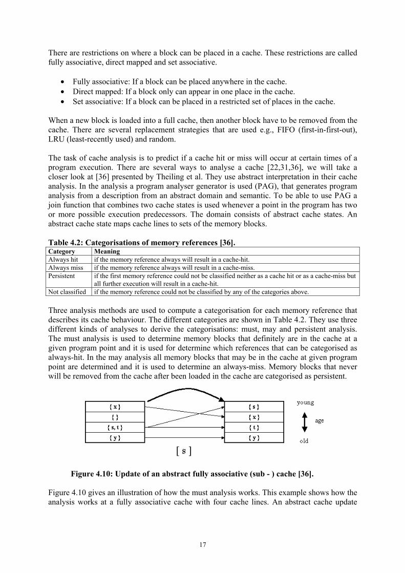
When a new block is loaded into a full cache, then another block have to be removed from the cache. There are several replacement strategies that are used e.g., FIFO (first-in-first-out), LRU (least-recently used) and random. The task of cache analysis is to predict if a cache hit or miss will occur at certain times of a program execution. There are several ways to analyse a cache [22,31,36], we will take a closer look at [36] presented by Theiling et al. They use abstract interpretation in their cache analysis. In the analysis a program analyser generator is used (PAG), that generates program analysis from a description from an abstract domain and semantic. To be able to use PAG a join function that combines two cache states is used whenever a point in the program has two or more possible execution predecessors. The domain consists of abstract cache states. An abstract cache state maps cache lines to sets of the memory blocks. Table 4.2: Categorisations of memory references [36]. Category Meaning Always hit if the memory reference always will result in a cache-hit. Always miss if the memory reference always will result in a cache-miss. Persistent if the first memory reference could not be classified neither as a cache hit or as a cache-miss but

all further execution will result in a cache-hit. Not classified if the memory reference could not be classified by any of the categories above. Three analysis methods are used to compute a categorisation for each memory reference that describes its cache behaviour. The different categories are shown in Table 4.2. They use three different kinds of analyses to derive the categorisations: must, may and persistent analysis. The must analysis is used to determine memory blocks that definitely are in the cache at a given program point and it is used for determine which references that can be categorised as always-hit. In the may analysis all memory blocks that may be in the cache at given program point are determined and it is used to determine an always-miss. Memory blocks that never will be removed from the cache after been loaded in the cache are categorised as persistent.

Figure 4.10: Update of an abstract fully associative (sub - ) cache [36]. Figure 4.10 gives an illustration of how the must analysis works. This example shows how the analysis works at a fully associative cache with four cache lines. An abstract cache update

17

function is used. Figure 4.10 shows how an abstract cache is changed when s is accessed, based on the LRU replacement strategy.

Figure 4.11: Join for the must analysis [36]. The join function that is used in the must analysis to combine two cache states is shown in Figure 4.11. A memory block stays in the abstract cache only if it is present in both operand abstract cache states. If a memory block has different ages in the two abstract cache states the oldest one is used. The final result is computed by the PAG to find out if a reference is an always-hit or not. 4.2.1.1 Loop analysis for caches Programs spend most of their run-time inside loops therefore the analysis of loops is an important part of the cache analysis. The first iteration of a loop often changes the cache contents i.e., memory blocks are loaded into the cache at their first access. In the following iterations most of the information has already been loaded into the cache. Therefore it is important to distinguish between the first iteration and the following iterations in a loop for a cache analysis. Theiling et al. [36] performs their cache analysis for loops by treating loops as procedures. This is shown in Figure 4.12.

Figure 4.12: Loop transformation [36].

18

They use a method called VIVU that virtually unrolls loops. The result of the VIVU approach is that memory references are considered in different execution contexts, making it possible to distinguish between the first and the following iterations of a loop. 4.2.2 Pipeline analysis In a pipelined processor overlaps between instructions occur to speedup the rate in which the CPU can process instructions. Pipeline analysis is used to model the execution time effects of such instruction overlaps. In this section we will first look at how a pipelined processor works, after that we will look closer at the pipeline analysis. 4.2.2.1 How a pipeline works Pipelining is used to speed up the CPU, instead of executing one instruction at a time, multiple instructions are overlapped in the execution. A pipeline consists of several stages, each stage completes a part of an instruction and the different stages operate in parallel. Compared to an unpipelined CPU, pipelining can under ideal conditions perform a speedup equal to the number of stages, but usually the speedup is lower due to instructions and resource dependencies.

Figure 4.13: Example of pipelined execution [16]. An example of how a pipeline works is shown in Figure 4.13. In this example the processor contains four stages. Instructions are fetched from memory in the IF stage. Integer and data memory instructions go through the EX stage, in this stage arithmetic operations are performed. Data memory is accessed in the M stage. In the F stage floating point instructions execute in parallel to integer and memory instructions. The time in clock cycles is shown on horizontal and the stages are shown on vertical. An instruction does not have to use all stages in a pipeline. Figure 4.13(a) shows three instructions that executes on a non-pipelined execution. An instruction in a non-pipelined execution CPU has to finish its entire execution before the next instruction can start its execution. The non-pipelined execution is finished in 10 clock cycles. In Figure 4.13(b) a pipelined execution is shown, instructions are overlapped and the execution is finished in only 6 clock cycles, which is 4 clock cycles less than in the non- pipelined CPU. The second instruction needs two clock cycles in the EX stage, this causing the third instruction to wait in the IF stage one cycle, this is called a pipeline stall. Two different kinds of pipeline stalls are structural hazards and data hazards. Structural hazard occurs if an instruction cannot enter its next stage because that the stage is used by another instruction, an example of a structural hazard is shown in Figure 4.13 (b). If an instruction requires data from a previous instruction that is not available yet because of the pipelining execution, then it is called a data hazard.

19

4.2.2.2 Hardware model To be able to analyse a pipelined processor a hardware model is used in almost all timing analysis approaches. A hardware model is a model of the actual processor where the program is executed. To be able to create a hardware model, detailed information of the timing behaviour of the processor has to be known. The difficulty to construct a hardware model grows with the complexity of the processor. To obtain the information of the processor is not always an easy task, for instance of competitive reasons processor manufactures often keep the internal of the core secret [16]. 4.2.2.3 Example of a pipeline analysis There are several ways to do a pipeline analysis [16, 22, 31]. We will now look at the presented by Engblom in [16]. This analysis is able to capture instruction interferences and overlaps between and inside basic blocks. The input to the analysis is a scope graph. As illustrated in Figure 4.14(a) the nodes of the scope graph consisting of basic blocks with execution scenarios attached. An execution scenario is information about how the instruction in the basic blocks should be executed e.g., a cache-hit or a cache-miss and could be the result of a cache analysis such as the one presented in 4.2.1. Individual nodes and sequences of nodes are executed through the hardware model.

Figure 4.14: Scope graph, timing model and timing graph [18]. The hardware model is treated as a black box i.e., the analysis does not need access to its internal. The hardware model returns the execution time of a node or sequences of nodes in the scope graph. The result is used to construct a timing model. An example of a timing model is shown in Figure 4.14(b). In a timing model tnode represent the execution time of one isolated node and δ seq represent the change in execution time that occur, due to the pipelining effect when nodes are executed in sequence. δ seq is a negative to indicate a speedup and δ seq is positive to indicate a slowdown. The timing model can handle hardware interference over several nodes. The result of the analysis can be represented in a timing graph as in Figure 4.14(c). In the timing graph the edges between the nodes represent the pipeline effect. 4.3 Calculation The result from the flow and low-level phases are used to calculate the final WCET estimate. There are three basic calculation methods presented in literature, tree-based, path-based and IPET (Implicit Path Enumeration Technique).

20

4.3.1 Tree-based Tree-based calculation is performed by using a bottom-up traversal of a syntax tree of the program. A syntax tree consists of different nodes and edges, there the leaf nodes represent basic blocks and the internal nodes represent the structure of the program e.g., if-statements or loops. To get the final WCET estimate of a program the tree is traversed bottom-up merging nodes into new nodes with a new time representing the WCET of the sub-tree. This is done with help of transformation rules.

Figure 4.15: Different calculation methods [18]. Figure 4.15(a) shows a control flow graph, it contains the timing behaviour of each node and also the maximal number of iterations. An example of how tree-based calculation works is shown in Figure 4.15(d). The transformation rules are used when traversing the syntax tree and nodes are merged into new nodes. Finally only one node is left with the estimated WCET of the program. One advantage with tree-based calculation is that it is computationally quite cheap, but because the computations are local within a single program statement it is problematic to handle long-reaching flow information and long hardware dependencies [18]. 4.3.2 Path-based In a path-based calculation, different paths in the program are calculated and together used to derive the overall path with the longest execution time. An example of how the path-based

21

calculation works is shown in Figure 4.15(b). Once again the calculation is based on the control-flow graph show in Figure 4.15(a). First the longest loop is found, after that the WCET is found by multiply the time for an iteration with the bound for the loop. The method can handle single loops but have problems with flow information reaching over larger program parts. 4.3.3 IPET IPET stands for implicit path enumeration technique and was first introduced by Li and Malik [29]. The calculation method expresses program flow and execution times using arithmetic constraints. Each basic block and program flow edge is given a xentity variable and a timing tentity. The xentity is a count variable representing how many times the given entity is executed and the tentity time represent the execution time cost of the entity. An example of how IPET calculation works is shown in Figure 4.15(c). The execution count variables of the start and exit nodes are both set to one, constraining the program to only start and exit once. Structural constraints are used to model possible program flows. To do that, the numbers of times a node can be executed are set to be equal to the sum of execution counts of its incoming and outgoing edges. For instance, for node B the following constraints are generated: xB = xAB = xBC + xBD The estimated WCET is found by maximising the sum: ∑ i є entities xi * ti The maximising problem can be solved using either ILP (Integer Linear Programming) or constraint programming. Constraint programming can handle more complex constraints than ILP, while ILP can only handle linear constraints but is usually faster. The advantage with IPET is that complex flow information can be expressed using constraints, but on the other hand it can also result in longer computation times and the result is also implicit. For example, if xC=95 and xD=5, means that C executes 95 times and D executes 5 times, but it is not possible to know in which order they executes. 4.4 WCET analysis tools In this section we look at different kinds of WCET analysis tools, both commercial and research WCET analysis tools are presented. 4.4.1 Commercial WCET analysis tools Bound-T [6] is a commercial WCET analysis tool developed by Space Systems Finland (SSF). It was first developed for the European Space Agency (ESA) and it has been used in space projects. The analysis is performed on executable code, so it is independent of source language (but not target hardware) and can handle programs written in different program languages. Some flow information can automatically be found on object code level using

22

Presburger arithmetic. The tool uses IPET for the calculation phase. Supported target processors are Intel 8051, ERC32/SPARC V7 and ADSP21020. AbsInt [1] is a company from Germany that develops tools for embedded systems and tools for validation, verification and certification of safety-critical software. The analysis is performed on executable code and the control flow of a binary program is reconstructed [37] and annotated with information needed by subsequent analysis. Microarchitecture analysis takes the annotated control flow graph as input. Abstract interpretation is used in the value analysis, cache analysis [36] and in the pipeline analysis. The value analysis determines ranges of values in registers that is used to find loop bounds and the analysis can in some cases detect infeasible paths. Integer linear programming is used in the path analysis. To allow a large number of different processors generic and generative methods are used whenever possible. Supported processors are ARM7, Motorola Star12/HCS12 and PowerPC 555. We will look closer at the AbsInt tool for the ARM7 processor in Section 5.2. 4.4.2 Research WCET analysis tools Mälardalen University and Uppsala University in Sweden and C-lab in Paderborn, Germany, have together developed a WCET analysis tool [18]. The structure of the tool is shown in Figure 4.16.

Figure 4.16: The structure of the Mälardalen University, Uppsala University and C-lab WCET tool [18]. The tool consists of several modules with well defined interfaces, making it easy to extend with new analyses and target processors. The modules are flow analysis, global low-level analysis, local low-level analysis (not shown in Figure 4.16) and calculation. The flow analysis module takes an intermediate code generated by a compiler as input. The result of the flow analysis is a scope graph annotated with flow facts that is passed to the low-level analysis and the calculation module. A basic block graph generated from the compiler is also an input to the low-level analysis. The result of the low-level analysis is a timing model. The timing model and the scope graph are given to the calculation module, which computes the final WCET estimate. Supported target processors are [16] NEC V850E and ARM9. The tool support three different kinds of calculation methods, path based, extended IPET and clustered [18]. Due to the

23

modular structure of the tool each calculation module can be chosen independently from the target processor. Heptane (Hades Embedded Processor Timing AnalyzEr) [24] is a research WCET analysis tool developed in France by the IRISA ACES team. The tool can analyse programs written in a subset of the programming language C e.g., the analysed code must not contain any goto statements or recursion. Loop annotations are required to be set manually and the tool uses tree-based calculation. Supported processors are: Pentium I, MIPS and Hitatchi H8/300. 4.5 Related work There have been some studies on industrial programs. Engblom [17] analysed the static aspect of a large number of commercial real-time and embedded applications to provide guidance for development of WCET tools. The analysis was performed with a modified C compiler and 334 600 lines of C source code was analysed. The conclusion of the analysis was that a complete WCET tool for industrial programs must handle following program features:

• Recursion • Unstructured flow graphs • Function pointers and function pointer calls • Data pointers • Deeply nested loops • Multiple loop exits • Deeply nested decision nests • Non-terminating loops and functions

Colin and Puaut [10] have studied the RTEMS real-time kernel to find out if the structure of the source code is suited for WCET analysis. RTEMS is a small real-time operating system for embedded applications. The analysis of RTEMS was performed with the WCET analysis tool Heptane that analyse programs written in the program language C. There was only a few number of loops in the analysed code and non of them where nested loops. The authors think that it was easy to find the loop bounds for 25 % of the loops. To find the remaining loop bounds required a deeper analyse of the source code. The analysed code did not contain any recursion and only a small number of dynamic calls. Colin and Puaut think that RTEMS is well suited for WCET analysis. Carlsson et al. [7] have analysed disable interrupt regions in the OSE operating system using a WCET analysis tool [18]. They build prototype tools to extract the disable interrupt regions, and construct a control flow graph from the extracted region. Not all regions could be found since it may be data dependent whether an instruction disable or enable an interrupt. Most of the analysed regions were very short, containing at most three basic blocks and only 5 % of the regions contained loops. They think that interrupt regions are well-suited for WCET analysis due to their simple code structure.

24

Rodriguez et al. [35] have used the Bound-T WCET analysis tool to derive WCET estimates of a Control and Data Management Unit (CDMU). The CDMU is an application in the CryoSat satellite from the European Space Agency. The experiment shows that it was difficult to bounding loops. One problem of bounding loops was when the compiler created a loop that did not exist in the source code. Their conclusion was that static WCET analysis can be used to derive WCET estimates for the CDMU application. However, they did not think static WCET analysis is mature to analyse the application fully automatically.

25

5. Industrial code and analysis environment In this section we will look at the industrial code that the analyses have been performed on, together with tools and other components used in the analyses. In section 5.1 OSE and the properties of its code will be described. Section 5.2 gives an overview of the aiT WCET tool. Section 5.3 presents the target processor ARM7TDMI together with supporting tools for debugging and simulation like the ARMulator. Finally, in Section 5.4 the ELF object code format that all WCET analyses have been performed upon is described. 5.1 Industrial code Most of the analyses have been performed on code from the OSE operating system from Enea. In 1968 four graduated technologists from Swedish Royal institute started Enea [13]. Enea has for a long time been one of the leading companies in computer technology. For instance Enea.se was the first registered domain name in Sweden. Also the first internet backbone in Sweden was administrated by Enea. They were also among the first to work with UNIX and object orientation. The real-time operating system OSE was developed by Enea in the mid-80s and the OSE Systems [32] that is a subsidiary of Enea, is market leader in real-time operating systems for communication infrastructure. The OSE operating system is used in many different applications including mobile telephones, medical equipments and in oil platforms. 5.1.1 The OSE operating system The OSE operating system is a real-time operating system supporting both hard and soft real-time code. In this section some properties of the OSE operating system is described in more detail. 5.1.1.1 Processes OSE contains different categories of processes that runs in parallel to perform specific tasks of the system. Most of the process types need to be assigned a priority value between 0-31, when the process is created. Value 0 is the highest priority and value 31 the lowest priority. Each process is always in one of following states: running state, ready state or waiting state. The different states are illustrated in Figure 5.1.

Figure 5.1: Process states [14]

26

Only one process can run on each CPU at the same time. Some of the code that the running process executes includes system calls, requesting a service from the operating system. The scheduler will perform a context switch if a process with higher priority than the running process becomes ready. If a process is ready and has lower priority than the running process, the process that is ready will then run as soon as the running process is finished. A process is in the waiting state if it is waiting for a event to occur or it is stopped. A processor could for example wait for a signal to arrive. The operating system supports five different types of processes: interrupt, timer, prioritised, background and phantom processes.

• An interrupt process is running in response to a hardware interrupt. An interrupt process can only be pre-empted by another interrupt process with higher priority.

• A timer process is usually invoked periodically to handle events. • A prioritised process must be assigned a priority when it is created. This priority is

often fixed, but can be changed by a system call. The prioritised process is the most common process type and is usually designed as a non-terminating loop.

• If no interrupt process, timer process or prioritised process is ready to run, then a background process is allowed to run.

• A phantom process has no program code and is never scheduled. The phantom processes are used as place holders.

5.1.1.2 Memory organisation In the OSE operating system, it is possible to grouping related processes together into blocks to form a subsystem. The processes in the same block use the same memory pool. Allocating memory from a pool is one of several ways to allocate memory in OSE, but it is the fastest way. The allocation can be performed with the alloc system call. The advantage with pools is that a memory block can have its own memory pool, which improves the robustness of the system, for instance if a pool gets corrupted, only the blocks connected to that pool is affected. The other processes that are not dependent of processes from the corrupted pool can continue to work as normal. Figure 5.2 illustrates the structure of allocating memory in a pool.

Figure 5.2: Memory Organisation [14]

27

The structure of a system is also improved, if processes are grouped into blocks. When the allocated memory is not needed anymore, the system call free_buf is used to free the allocated memory [14]. 5.1.1.3 Signals The simplest way to send a message from a process to another is performed by sending a signal. All signals contain at least a signal number, data contents, owner, size, sender and addressee. The owner of a signal buffer can be changed from the sending process to the receiving process by the send system call. The receive system call can by looking at the signal number determine the type of signal that is sent to it, and see if it is the kind of message the process is looking for. The size of a signal buffer must be allocated from a pool before a signal can be used. Only the memory restricts how many signals a system can have [14]. 5.1.1.4 Disable interrupt regions In critical parts of the code disable interrupt regions are used, for instance when a shared resource is accessed. When the region is entered the interrupts are turned off, and enabled when leaving the region. Disable interrupt regions are often very short, so that waiting processes are not delayed for a long time. The analyses have been performed at real-time classified system calls and on disable interrupt regions of the OSE code. 5.2 The aiT WCET analysis tool In this section the aiT WCET analysis tool is described. The aiT WCET analysis tool has been used to calculate WCET estimates for the ARM7TDMI processor. The tool is developed by AbsInt [1], a company developing tools for embedded systems and tools for validation, verification and certification of safety-critical software. The structure of the aiT tool is illustrated in Figure 5.3.

Figure 5.3: The structure of the analysis [1].

28

The analysis is performed on executable binary code from which the control flow is extracted and annotated [37] with information. Abstract interpretation is used in the value analysis, cache analysis [36] and in the pipeline analysis. The value analysis determines ranges of values in registers that are used to find loop bounds and can in some cases also detect infeasible paths. The ARM7TDMI processor is an uncached core, and therefore no cache analysis is used for this processor. Integer linear programming is used in the path analysis. To allow a large number of different processors generic and generative methods are used whenever possible. 5.2.1 Annotations To improve the analysis aiT allows the user to manually provide extra information (annotations) [19]. This information can be specified in two help files, AIP and AIS. The AIP file contains memory specifications and restrictions of the analysis. In the AIS file annotations can be specified to help the tool in the analysis and to improve the results. 5.2.1.1 Memory specifications and restrictions When a program is executed on a real hardware, then an instruction can have different access time depending on where in the memory it is stored. Therefore one has to specify the access time of different memory areas to be able to perform the analysis for the specific hardware. An example of such annotation is: MEMORY_AREA: 0x8000000 0xFFFFFFFE 1:1 2 READ&WRITE DATA-ONLY This example shows that it takes 2 clock cycles to read and write data in the specified area, starting at address 0x80000000 and ending at address 0xFFFFFFFF. If the analysed code contains many loops, then a program point in the value analysis can be called from an enormous amounts of different paths, which takes very long time to analyse but can improve the quality of the results. To speedup the analysis the following annotations can be used: INTERPROC: vivu4 Interproc_N: n Interproc_MAX_CUT: m The first annotation vivu4 (Virtual Inlining Virtual Unrolling) makes it possible to find loop bounds automatically. The second restricts the calling depth to the number of n. The analysis uses an unlimited calling depth if n is set to zero. The last annotation restricts the number of abstract values (contexts) to m, that is calculated for a loop. For example, if function foo(x) is called twice. In the first call the value of x is 1, and in the second call x has the value of 4. Then a safe approximation is to assume that the value of x is in the interval [1..4] for each call to foo. The precision would be improved if instead a single abstract value is calculated for each call, then x will be in the interval [1..1] for the first call and in the interval [4..4] for the second call. 5.2.1.2 Control flow annotations This section explains some annotations that have been used in the analyses and are written in the AIS file. A word with capital letters indicates a keyword in the annotations. The ProgramPoint represents the address of an instruction. If a path is infeasible in the analysed code, then following annotation can be used to exclude the path from the analysis.

29

SNIPPET ProgramPoint IS NEVER EXECUTED; If a condition in the code is always true, than the condition annotation is used. CONDITION ProgramPoint IS ALWAYS TRUE; In this case the false path of the condition is excluded from the analysis. It is also possible to set a condition to be always false too. The flow annotation is a way to specify how a many times a basic block is executed compared to another basic block. FLOW ProgramPointA / ProgramPointB MAX 3; In this case basic block A is executed 3 times more than basic block B. An example of the use of this annotation is to annotate loop bounds for loops with several entries. To specify the target of a branch that cannot be found automatically then following annotation is used: INSTRUCTION ProgramPoint BRANCHES TO Target1, …, Targetn; The following annotation is used for code that you do not want to analyse: SNIPPET ProgramPoint IS NOT ANALYSED AND TAKES MAX n CYCLES; Then the code is removed from the analysis. It is also possible to manually specify loop bounds. An optional qualifier indicates if the loop test is at the beginning or at the end of the loop. The qualifier refers to the executable since the loop test can be moved after the compilation. LOOP “_prime” + 1 LOOP END MAX 10; In this example the first loop in the function _prime is executed at most 10 times and the loop test is at the end. Loop bounds can also be specified directly in the source code. The source code annotations must be written as comments, and start with the keyword ai. The comments also contains the keyword here, that denotes where the annotation occur. The code must be recompiled when a line is added or deleted, because the line information is created by the compiler. Loop annotations in the source code can be written anywhere inside the loop, for instance: for (i=3; i*i <=; i += 2){ if (divides (i, n)) /* ai: loop here end max 10; */ return 0; } There are also other kinds of annotations e.g., upper bounds of recursive calls and to set the clock rate of the microprocessor.

30

5.1.2 Example of a program analysis When the tool is started, four different windows are visible, files, messages, source and disassembly windows. These windows are shown in Figure 5.4. In the files window different files are included to be able to perform the analysis. The files window is divided into two parts, executable and supporting files. The code will be analysed needs to be specified, this could be given either in .out files in COFF formats or in ELF files. The start point of the analysis also needs to be specified i.e., the start address of the analysis. It is possible to type the name of the routine where the analysis should start and it is also possible to specify the address of an instruction if the start point is not a routine entry.

Figure 5.4: Files, Messages, Source and disassembly windows. In the supporting files section an AIP file has to be selected (Section 5.2.1.1). To help the analyser in the flow analysis, manually annotations can be specified in the AIS file (Section 5.2.1.2). The reporting file shows messages and the WCET results of the analysis. The source window shows error and warning messages. It is possible to click on a message and then the corresponding line in the message window will be highlighted, e.g., if a loop bound is missing, the related loop in the source code will be displayed. From a selected entry point, the tool computes a combined call graph and control flow graph. When the combined call graph and control flow graph is first displayed, then only the call graph is visible. The call graph shows the overall structure of the code that is analysed, where the nodes in the call graph represents routines and loops. A node in the call graph can be extracted to show the control flow graph of the routine and in each basic block it is possible to view the instruction sequences of the basic block. The combined call graph and control flow graph can be generated in three different ways; compute CFG, analyse and visualise. Compute CFG is used to in a fast way get an overview of the structure of the program and no WCET or loop bound analysis is performed. Analyse performs a full WCET analysis and visualise shows the pipeline analysis.

31

Here is an example of how a WCET analysis of a program can be performed. The source code of the program to be analysed is shown in Figure 5.5.

Figure 5.5: Example code. In this example the loop in the routine has a manual loop bound annotation written in the source code (source code annotations are not yet supported for analyses on ELF files). The loop can iterate at most 357 times and in the executable the loop test is at the end. When the menu item analyse, is chosen from the action menu, the WCET result and the combined call graph and control flow graph is shown as illustrated in Figure 5.6.

Figure 5.6: WCET result and call graph The WCET result is shown in both clock cycles and in milliseconds, but if no clock rate is specified then only the result will be obtained in clock cycles. In the combined call graph and control flow graph red edges indicates if a routine or basic block is on the WCET path. In Figure 5.6 the only routines that are not on the WCET path are the routines loop_0000 and IND_CALL. The dotted border of routine IND_CALL indicates that the routine contains computed calls that have not been resolved.

32

For each node on the WCET path it is possible to view a predicted WCET contribution and calling context, as illustrated in Figure 5.7.

Figure 5.7: WCET Contribution and contexts The predicted WCET contribution is the sum of the estimated WCETs of all routine invocations along the WCET path.

Figure 5.8: Control flow graph. A routine node in the call graph can be extracted to show the control flow graph of the routine, this is shown in Figure 5.8. In this case the corresponding source code is shown in the control flow graph1. The maximum worst-case traversal for an edge taken over all contexts is indicated by max #. The maximum time taken over all contexts indicates with max t.

33

1 The source code view, is only working for .out executables so far.

Figure 5.9: Pipeline states. It is possible to view the pipeline state of the WCET analysis if visualise is chosen from the action menu. By selecting a basic block from the combined call graph and a context from the control flow graph, a pipeline state is shown. An example of a pipeline state is shown in Figure 5.9. The pipeline state lists the instructions of the basic block where each instruction consists of a list of operations. 5.3 ARM In this section the target hardware ARM7TDMI is described with complementary components used with the processor. ARM7TDMI is manufactured by ARM limited, which is market leader for low-power and cost-sensitive embedded applications. ARM processors are Reduced Instruction Set Computers (RISC). When the first RISC processor was developed in the beginning of 1980s, the idea was that the optimal architecture for a single-chip processor does not have to be the same as for a multi-chip processor. The architecture of a RISC processor is simple and is cheaper to design than CISC (Complex Instruction Set Computers) processors. One drawback with RISC is that it has poor code density compared with CISCs. 5.3.1 The ARM7TDMI processor The ARM7TDMI processor is designed for cost and power sensitive products, and is today the most widely used 32-bit embedded RISC microprocessor solution. Examples of applications that use an ARM7TDMI processor are mobile telephones, personal digital assistants and modems. The ARM7TDMI is forward compatible with ARM9, ARM10 and Strong ARM [5]. The name ARM7TDMI stands for ARM7, a 3 volt compatible rework of the ARM6 32-bit integer core. T stands for Thumb instruction set (see Section 5.3.1.1.1), D stands for debug support, M stands for an enhanced Multiplier and I stands for embedded ICE (see Section 5.3.2.1). Figure 5.10 shows the organisation of ARM7TDMI, with a processor core, a bus splitter that separates data and an embedded ICE module and a JTAG controller that is used for debugging [20].

34

Figure 5.10: ARM7TDMI organisation [20] 5.3.1.1 The ARM7TDMI architecture The ARM7TDMI is an uncached core with a 3-stage pipeline, where the pipeline stages are fetch, decode and execute. It has four basic types of memory cycles: internal, non-sequential, sequential and coprocessor register transfers. Most of the instructions are executed in a single clock cycle. ARM has two ways to store words in the memory, little endian and big endian, depending on whether the least significant byte is stored at a lower or a higher address than the next most significant byte. 5.3.1.1.1 The ARM and Thumb instruction sets The ARM7TDMI processor supports two different instruction sets, ARM and Thumb. The ARM instruction set contains instructions that are 32-bit wide and aligned on a 4-byte boundary. It use 3-address data processing instructions i.e., the result register and the two source operand registers are independently specified in the instruction. In the ARM instruction set that is used in ARM7TDMI, all instructions are conditionally executed. The Thumb instruction set is used to improve the code density. The Thumb instruction set has instructions of 16-bit length and can be viewed as a compressed form of the ARM instruction set. It is not a complete architecture, so Thumb systems needs to include ARM code even if it is only used to handle initialisation and exceptions. An embedded Thumb system often have ARM code in speed-critical regions, but the main part of the system will be Thumb code. Which mode the ARM processor will execute depends on bit 5 in the Current Program Status Register (CPSR), the T bit. The processor interprets the instruction stream as Thumb instructions if the T bit is set otherwise the processor interprets the instructions as ARM instructions. The differences between the ARM instruction set and the Thumb instruction set are:

• All ARM instructions are executed conditionally and most Thumb instructions are executed unconditionally.

• ARM instructions use a 3-address format and Thumb instructions use a 2-address format.

• As a result of the dense encoding, Thumb instruction formats are less regular than ARM instruction formats.

35

The two instruction sets have different advantages. If it is used in an application there performance is most important, then the system should use a 32-bit memory with ARM code. A 16-bit memory system with Thumb code may be used if cost and power consumption is more important. A comparison between Thumb code with pure ARM code gives [20]:

• The Thumb code requires 70% of the space of the ARM code. • 40 % more instructions are used in Thumb code than in ARM code. • The ARM code is 40 % faster than the Thumb code with 32-bit memory. • The Thumb code is 45 % faster than ARM code with 16-bit memory. • Thumb code uses 30% less external memory power than ARM code.

The analysed OSE operating system contains both ARM and Thumb code. The ARM7TDMI supports seven different operating modes: user mode, fast interrupt mode, supervisor mode, abort mode, interrupt mode and undefined mode. The programmer can only change the state of a program in user mode. The registers r0-r14 and r0-r7 are registers for general purpose of ARM instructions and Thumb instructions respectively. In both instruction sets register r15 is the program counter. 5.3.1.1.2 Classes of instructions In both the ARM and Thumb instruction sets, instructions can be divided into four classes, data processing instructions, load and store instructions, branch instructions and coprocessor instructions. Data processing instructions changes the value in a register with arithmetic or logical operations. At least one of the two source operands must be a register, the other operand can be an immediate value or a register value. The result in a multiply instruction can be a 32-bit result or a long 64-bit result. Load and store instructions can transfer a 32-bit, a 16-bit or a 8-bit between a memory and a register. Load and store instructions allow single or multiple registers to be loaded or stored at one time. A branch instruction can branch from one place in the code to another. One branch instruction is branch with link (BL), that makes it possible to branch to a subroutine in a way which makes it possible to resume the original code sequence when the execution of the subroutine is completed. Another branch instruction is branch and exchange (BX) that switches between ARM and Thumb instruction sets. There are three different kinds of coprocessor instructions: data processing, register transfer and data transfer instruction. Coprocessor data processor instructions are internal, and cause a change in the coprocessor registers. A processor value can be transferred to or from an ARM register with coprocessor register transfer instructions. Data can be transferred to and from the memory with coprocessor data transfer instructions [5]. 5.3.2 Debug support It is more complicated to debug an embedded system compared to a non-embedded system, because there is probably no user interface in the embedded system. ARM7TDMI implements an Embedded ICE module that uses a JTAG controller for debugging.

36

5.3.2.1 Embedded ICE In-Circuit Emulator (ICE) is a method for debugging embedded systems. This method is based on that the processor in the target system is replaced with an emulator that can be based around the same processor chip, but contains more pins, that makes it easier to debug a program. Breakpoint and watchpoint registers are controlled through the JTAG test port. With help of the registers, it is possible to halt the ARM core for debugging. 5.3.2.2 JTAG system Most of the ARM designs have a JTAG system for board-testing and on chip debug facilities. For testing a printed circuit board the JTAG boundary scan can be used, and it is a test standard developed by the Joint Test Action Group. If a printed circuit board have a JTAG test interface, then outputs can be controlled and inputs observed independently of the normal function of the chip. 5.3.3 ARM development tools The ARM development tools are intended for cross-development i.e., they run on different architecture from the one which they produce code. For example it is possible to develop the program on a PC running Windows or on a UNIX platform and then download the executable on the target platform, which improves the environment for software development. The overall structure of the ARM cross-development toolkit is shown in Figure 5.11.

Figure 5.11: The structure of the ARM cross-development toolkit [20] The toolkit consists of an ANSI C compiler that can produce ARM object format (.aof). The C compiler can also produce assembly source output, so that the code can be inspected or hand optimised, Thumb code can also be produced.

37

The ARM assembler is used to produce .aof files. A linker is used to combine one or more object files that have been produced by the C compiler or the ARM assembler into an executable program. The linker can produce debug tables and if the object files where compiled with full debug support, a program can be debugged using variable names in the program. 5.3.3.1 Debugging tools Two debugger interfaces used in the ARM toolkit are the ARM symbolic debugger (ARMsd) and the AXD (ARM extended Debugger). The debugging of a program can be performed under emulation, for instance with help of the ARMulator. It is also possible to debug a program remotely, for instance on the ARM development board. A program can be downloaded to the ARMulator or the development board and then it is possible with help of setting breakpoints to examine the behaviour of a program. 5.3.3.2 The ARM development board The ARM development board is a circuit board that includes an ARM core and different components and interfaces to support development on ARM-based systems. Debug protocols are connected to the board either via a serial line or JTAG test interface. Memory components and electrically programmable devices can be configured to emulate application-specific peripherals. We tried to use a development board in this thesis. Unfortunately it turned out to be harder to extract any timing results from the hardware than we thought from beginning. Therefore the hardware simulator, ARMulator was used instead. 5.3.3.3 The ARMulator The ARMulator is a simulator, which makes it possible to evaluate the behaviour of a program for a certain ARM processor without using the actual hardware. A software model of a system can be build that can include a cache, memory management unit, peripheral devices, operating system and software. The ARMulator consists of four main components [3]:

• The ARM processor core model that handles the communication with the debugger. • The memory system, there the memory interface transfers data between the ARM

model and the memory model or memory management unit. It is possible to modify the memory model, for instance peripheral registers and memory mapped I/O. Modelling of different RAM types and access speed can be modelled in a map file.

• The coprocessor interface that supports custom coprocessor models. • The operating system interface, which makes it possible to simulate an operating

system. It is possible to measure the number of clock cycles of a program using the ARMulator. Bus and core related statistics can also be obtained from the debugger. The statistics vary depending on which architecture the processor is based on. The ARM7TDMI uses a single bus for both data and instruction access, so the cycle types refer to both types of memory access. The statistics produced for the ARMTDMI processor are:

• Sequential cycles (S-cycles). • Non-sequential cycles (N-cycles). • Internal cycles (I-cycles). • Coprocessor cycles (C-cycles). • Total, is the sum of the S-cycles, N-cycles, I-cycles and C-cycles.

38

There is no guarantee that the model of an ARM processor corresponds exactly with the actual hardware. However, since ARM7TDMI is not a very complex and uncached core, the ARMulator should be rather cycle accurate [4]. The total number of clock cycles produced by the ARMulator was compared against WCET estimates (see Section 6.3 and Section 6.4). 5.4 Object code The aiT WCET tool performs WCET analysis on object code level. Therefore we will now look at the ELF object code format used for all analyses. First, we will look at the overall structure of an object code format, then study the ELF object code format in detail. Object files are created by compilers and assemblers and the files contains binary code and data created from source file. A linker combines multiple object files into one and the executable is loaded into the memory by a loader. Usually the object code format contains five kinds of information:

• Header information: Gives the overall information about the file, and contains information about the size of the code, the name of the source file and the date the file was created.

• Object code: Is generated from the compiler or assembler and consists of binary instructions and data.

• Relocation: A list of places in the object code that have to be fixed up when the linker changes the address of the object code.

• Symbols: Defines global variables. • Debugging information: Information that is used to debug a program, and contains

information that is not needed for linking e.g., source line information, local symbols and description of data structures used by the object code.

5.4.1 The Executable and Linking Format (ELF) The ELF format was developed for UNIX systems, and is more powerful and more flexible than the previous object file formats, such as a.out and COFF (Common Object File Format). There are three different kinds of ELF files: relocatable, executable and shared object. Relocatable files are created by compilers and assemblers and needs to be processed by a linker before runtime. All relocation are done in the executable files and all symbols are resolved except perhaps shared library symbols that could be resolved at runtime. Shared objects are shared libraries that contain both symbol information for the linker and directly runnable code at runtime.

39

Figure 5.11: The structure of an ELF file [28] The structure of an ELF file is illustrated in Figure 5.11. An ELF file always starts with an ELF header. The ELF header describes the type of the object file, the version and the target architecture. Depending on if it is an executable file or not, decides if the file contain segments or sections. Both relocatable and shared object files are considered to be a collection of sections. A section contains a single type of information e.g., program code, read-only, read-write, relocations entries and or symbols. An ELF executable file has segments that contain information, for instance read-only code, read-only data and read-write data. The loadable sections are packed into the appropriate segments, so the system can map the file with one or two operations. The debug information format DWARF is used for ELF files. DWARF makes it possible to use a compiler to debug the object code referring to source function and variable names, and also to set breakpoints [28]. The analyses in this thesis have been performed on ELF executable files.

40

6. Experiments In this section the result of our experiments are presented. First the result from the analyses of system calls is presented, followed by the result of the analyses of disable interrupt regions. After that a comparison between estimated WCET results produced by the aiT WCET analysis tool and a hardware simulator is given. Finally we will look at how the analysis with the WCET tool is affected by different levels of compiler optimisations. 6.1 Analysis of system calls This section presents the results of the WCET analyses on some OSE system calls. The analyses have been performed on the system calls with three different system configurations. This section gives the result of the analyses that have been performed on code with error checks enabled and with advanced memory protection (see Appendix for more results). The four analysed system calls are: alloc, free_buf, receive and send. They are real-time classified system calls in the OSE operating system. A short description of the system calls is given in Table 6.1. For a more detailed description see Section 5.1. Table 6.1: A description of the analysed system calls System call Description Alloc Allocation of memory in a pool. Free_buf Free allocated memory. Receive Receive a signal from another process. Send Sends a signal from a process to another process. In each analysis, the code has been compiled with the ARM C compiler. The memory in the WCET analysis tool was set to zero-wait states i.e., an instruction will be executed in same number of clock cycle no matter where in the memory the instruction is stored. The estimated WCET results are given in clock cycles. Table 6.2 describes the different analyses that have been performed. Table 6.2: Description of the analyses System call Restrictions of the analysis Assumptions Alloc (a) Buffers of correct size exist. Alloc (b) No buffers of correct size exist.

No swap out handler is registered.

Free_buf There are two pools in the system. Receive (a) Receive all signals. The signal is first in the queue. No swap out

handler is registered. A 20 bytes signal is copied and no redirection.

Receive (b) Receive a signal. The signal is in at second place in the queue. Max 2 buffers before in the queue. No swap out handler are registered. A 20 bytes signal is copied. No redirection.

Send (a) Send a signal to a process with higherpriority.

The call to int mask handler is not analysed. No swap out handler are registered and the analysis stops before the interrupt process is called. No redirection

Send (b) Send a signal to a process with lower priority.

No redirection.

The analyses of the system calls were restricted to some specific program behaviours instead of analysing the entire code. Therefore alloc, receive and send have been analysed two times, represented by (a) and (b) in the system call column. To make the results of the analyses more useful, only normal program behaviours were analysed i.e., we assume that no errors occurs.

41

The rightmost column shows assumptions that were made to represent normal program behaviours. In Table 6.3 the estimated WCET result is presented for each analysis. All columns show the result after that the paths that should not be analysed have been removed from the analysis. The first column shows the name of the analysed code (System call). The next column shows the number of routines displayed by the aiT WCET tool (# Routines). The number of assembly instructions in the analysis is also given (Size). Followed by the number of basic blocks (# Blocks) and the number of loops (# Loops) in the analysis. The number of annotations used in the analysis is given (# Annotations), and finally the WCET estimate for each analysis is given in clock cycles (WCET (cycles)). Table 6.3: The results of the system calls analyses System call # Routines Size # Blocks # Loops # Annotations WCET (cycles)Alloc (a) 1 78 15 0 10 127 Alloc (b) 9 390 54 0 18 433 Free_buf 2 100 19 0 15 186 Receive (a) 15 531 119 2 29 821 Receive (b) 17 609 143 4 33 1469 Send (a) 4 281 56 0 32 493 Send (b) 5 288 62 0 33 417 All estimated WCET results are calculated with all paths leading to an error handling routine excluded from the analyses. The reason is that error handling code can take very long time compared to the normal execution. This was done by setting a condition annotation to be always true or false or setting a basic block to not be executed (see Section 5.2.1.2). The system call send exemplifies how removed paths can affect the control flow graph. With no annotations the system call consists of at least 39 routines (it contains a couple of unresolved branches that can make the control flow graph even bigger). When the analyses of send (a) and send (b) were finished only 4 respectively 5 routines were left. This also explains the large number of annotations required for the two send versions. A few loops were also analysed. We will look closer at two of them. The first loop appears in both the analyses of receive. The loop iterates through an array with signal numbers. The number of times the loop iterates depends on which signal a process wants to receive. Theoretically the loop can iterate over 32000 times, but not practically. Each iteration of the loop takes 13 clock cycles. The loop can have a big impact of the WCET estimate depending on which loop bound that is set. The WCET of the loop depends on the number of signals in the system.

Figure 6.1: The total WCET estimates affected by the number of loop iterations Another example of a loop that have been analysed appears in receive (b). Its behaviour is illustrated in Figure 6.1, which shows how the five first iterations of the loop affect the total

42

WCET estimates. The loop iterates through a queue of signal buffers. The characteristics of the loop, is similar as the previously explained loop. The WCET for one iteration is 182 clock cycles. Depending on how many signal buffers that are before in the queue decides the number of times the loop will iterate. It is difficult to statically determine the number of signal buffers that are in the system. Therefore, this loop was set to have a loop bound that represents a normal execution. The overall system call analyses were quite time consuming, even if the codes that finally were analysed became rather small. The main reason was that we first tried to correct all the warnings that occurred in the analyses e.g., unresolved branches and loop bounds. Other things that affected the time of the analyses was that we did not really know from the beginning what parts of the code that should be executed in the normal case. To summarise; we think the code that were analysed are suitable for performing WCET analysis upon. However, some of the analyses does not have a fixed WCET, it could depend on the dynamical behaviour of the system and on system states. Therefore, to be able to perform the analyses requires a detailed knowledge about the system e.g., cooperate closely with the programmers of the operating system. 6.2 Analysis of disable interrupt regions Another part of the OSE operating system that has been analysed is disable interrupt regions. A disable interrupt region is executed for critical parts of the code e.g., when shared resources are accessed. When a disable interrupt region is executed, then the executing process cannot be interrupted before the region is left. The regions are often very short, so that other processes are not delayed to long. Several disable interrupt regions can share the same parts of the code, making two regions having the same start address but different end addresses or vice versa. This indirectly means that some parts of the code are analysed more than once. The purpose of performing analyses on disable interrupt code is that if all regions are extracted from the source code, then it is possible to use a WCET analysis tool instead of measurements. But not all regions can be extracted from the source code at the moment. Disable interrupt regions have been analysed before in a Master’s thesis by Martin Carlsson [8]. His work differs from ours in that the target processor used was ARM9 (not ARM7TDMI) and the analysis was performed on different executable (due to different compilations of the code). To extract the disable interrupt regions from the code a tool called WCET-prepare was used and the same tool that was used by Carlsson. An overview of the performed analysis is given in Figure 6.2.

43

Figure 6.2: An overview of the analysis Each function in the source code is filtered, searching for disable interrupt regions. With help of the ELF file the physical starting address is given for each function. For each disable interrupt region a basic block graph was built and placed into a TCD (Textual Code Description) file. After that it was easy to manually transform the program behaviour of each region into annotations for the WCET analysis tool, and finally produce WCET estimates. Totally 180 disable interrupt regions were analysed. The majority were very short and not so complex, in total 132 the regions contained five or less basic blocks. Therefore not so many annotations were used for each analysis. Figure 6.3 illustrates the number of annotations that were used.

Figure 6.3: The number of annotations As we can see, the majority of analysis needed only a few annotations. Totally, 119 of the 180 analyses needed only two or less annotations. We will now take a closer look at some of the regions that have been analysed. Figure 6.4 shows illustrative examples of three different regions that have been analysed.

44

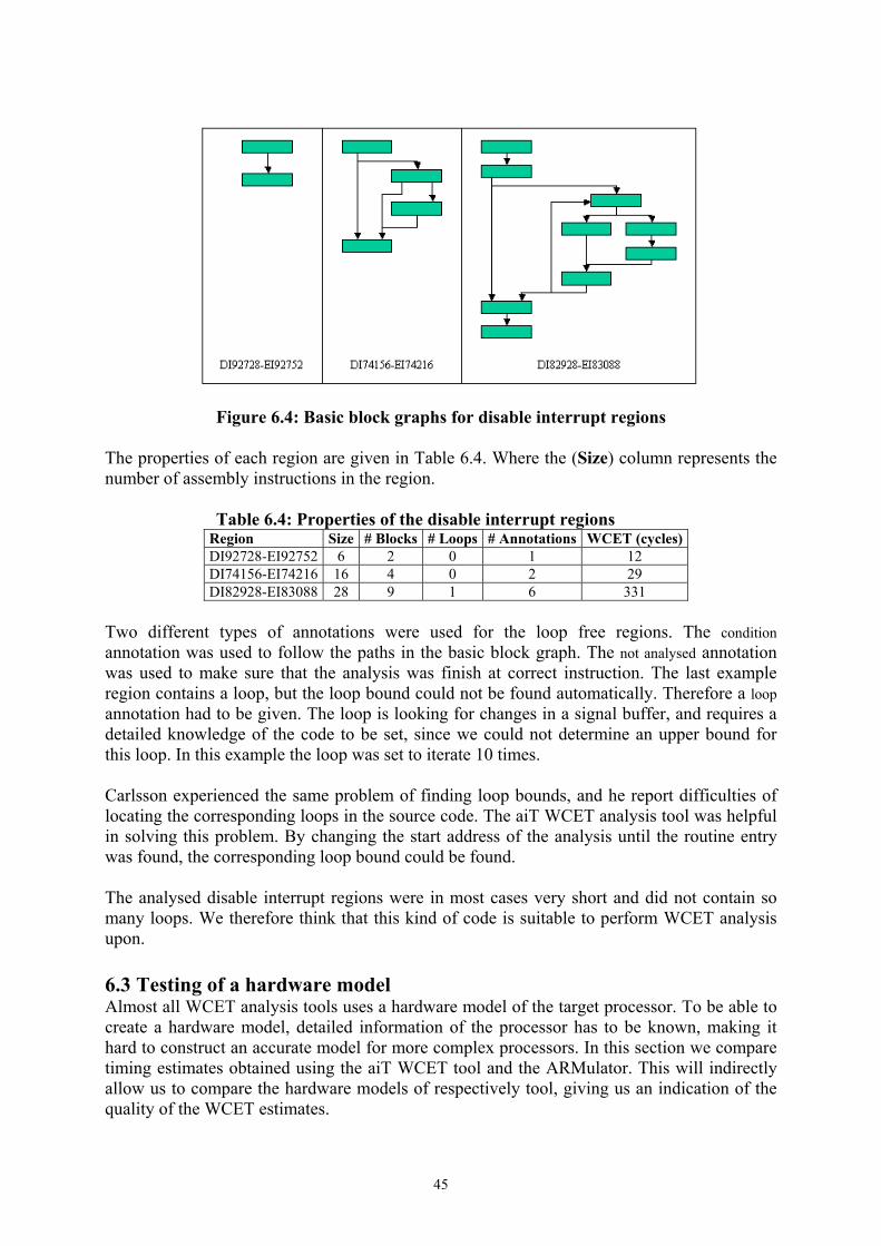
Figure 6.4: Basic block graphs for disable interrupt regions The properties of each region are given in Table 6.4. Where the (Size) column represents the number of assembly instructions in the region. Table 6.4: Properties of the disable interrupt regions

Region Size # Blocks # Loops # Annotations WCET (cycles) DI92728-EI92752 6 2 0 1 12 DI74156-EI74216 16 4 0 2 29 DI82928-EI83088 28 9 1 6 331

Two different types of annotations were used for the loop free regions. The condition annotation was used to follow the paths in the basic block graph. The not analysed annotation was used to make sure that the analysis was finish at correct instruction. The last example region contains a loop, but the loop bound could not be found automatically. Therefore a loop annotation had to be given. The loop is looking for changes in a signal buffer, and requires a detailed knowledge of the code to be set, since we could not determine an upper bound for this loop. In this example the loop was set to iterate 10 times. Carlsson experienced the same problem of finding loop bounds, and he report difficulties of locating the corresponding loops in the source code. The aiT WCET analysis tool was helpful in solving this problem. By changing the start address of the analysis until the routine entry was found, the corresponding loop bound could be found. The analysed disable interrupt regions were in most cases very short and did not contain so many loops. We therefore think that this kind of code is suitable to perform WCET analysis upon. 6.3 Testing of a hardware model Almost all WCET analysis tools uses a hardware model of the target processor. To be able to create a hardware model, detailed information of the processor has to be known, making it hard to construct an accurate model for more complex processors. In this section we compare timing estimates obtained using the aiT WCET tool and the ARMulator. This will indirectly allow us to compare the hardware models of respectively tool, giving us an indication of the quality of the WCET estimates.

45

In the experiments, the memory configuration in the aiT tool was set to zero wait-states The ARMulator was set to use the default memory model with 4 GB of zero wait-states RAM. The benchmarks programs used in the experiments are small and have no conditional constructs i.e., no if-statements exist in the code. The code was compiled with the ARM C compiler with minimum optimisation for space. Most of the benchmarks are from a subset of the DSPstone fixed-point kernel [12] and a description of all benchmarks used in the experiment is given in Table 6.5. Table 6.5: Description of hardware model benchmarks.

Program Description Size # Blocks # Loops Biquad_one_section Performs the filtering of input values through

a biquad IIR section. 54 5 0

Complex_multiply Performs a single mac operation on complex values

56 4 0

Complex_update Implements the operation d=c+a*b 38 4 0 Convolution Convolution filter. 31 13 2 Dot_product Computes a dot product of two vectors. 25 9 1 Fir Digital filter. 43 14 2 Ims Performs a finite-impulse-response filtering. 80 19 3 Matrix1 Computes the matrix product of 3x3 matrix

and a 3x1 vector. 77 34 6

Matrix2 Computes the product of two matricies. 84 34 6 Matrix3 Computes the product of two matricies. 27 11 2 N_complex_updates Updates an array of data. 74 14 2 N_real_updates Updates an array of real data. 46 13 2 Real_update Implements the operation d=c+a*b. 16 4 0 Fir2dim Perform the convolution of a input matrix and

a cofficient matrix. 158 69 13

Fibcall Simple iterative Fibonacci calculation, Used to calculate fib(30).

26 9 1

Matmult Matrix multiplication of two 20x20 Matrices.

60 28 5

The number of assembly instructions in the analysis is given (Size). Followed by the number of basic blocks (# Blocks) and the number of loops (# Loops) in the analysis. To be able to count the number of clock cycles, two breakpoints were set in the ARMulator. The first breakpoint was set on the first instruction of the analysed code and the second breakpoint on the last instruction of the analysed code. At the starting point of the analysis, the pipeline state could be different between the ARMulator and the WCET analysis tool. This is because the ARMulator executes a start up code before the first instruction in the analysed code is executed. Different pipeline states can only affect the total result with a few clock cycles and therefore the ratio in any larger program is not affected. The result of the experiments is shown in Table 6.6.

46

Table 6.6: Results of the hardware model experiments. Program ARMulator aiT Ratio

Biquad_one_section 150 167 1.11 Complex_multiply 172 190 1.10 Complex_update 104 121 1.16 Convolution 660 703 1.07 Dot_product 95 108 1.14 Fir 978 1022 1.04 Ims 1520 1598 1.05 Matrix1 37887 39900 1.05 Matrix2 34787 36800 1.06 Matrix3 317 345 1.09 N_complex_updates 2399 2539 1.06 N_real_updates 1263 1307 1.03 Real_update 55 66 1.20 Fir2dim 7096 7401 1.04 Fibcall 522 532 1.02 Matmult 5185 5442 1.05

The first two columns give the results in clock cycles, for each tool. In the last column the ratio between the two results is shown. The result shows that the larger benchmarks have a lower ratio i.e., overestimation, than the smaller benchmarks. Probably it could have something to do with interpretation of the start or the end of the analysis and a few extra clock cycles affect the ratio more for small program than larger program where the ratio is about 1.05. The aiT tool produced in all cases estimates that were higher than the simulated results. We think this is positive, because it gives an indication that the WCET estimates are safe. It should finally be noted that the WCET estimates have been compared against another hardware model and not against the real hardware. 6.4 How optimisations affects the WCET results When developing embedded systems both the size and speed are important parameters. Programs are therefore often compiled with different optimisation levels, depending on the use of the program. In this section we will investigate how the WCET analysis and estimated results are affected when a program is compiled with different optimisations and compilers. Two different compilers were used in the experiment, the ARM C compiler [2] and the ARM7TDMI IAR compiler [25]. With help of the two compilers, benchmarks were compiled with different optimisations. Each benchmark was compiled for size and speed with medium and maximum optimisation levels. The number of contexts in the analyses needed to be restricted. Because when the analysed code contains several loops then the number of contexts can become very large. The number of loop contexts was restricted to four and the calling depth to seven (see Section 5.2.1.1). But this should not affect the result of the analysis, because in conditional constructs the flow annotation was used to set the number of times a basic block was executed. Table 6.7 illustrates the optimisations used for the IAR compiler.

47

Table 6.7: Enabled optimisations for the IAR compiler. Optimisations Description Remarks

Common sub-expression Elimination

Redundant re-evaluation of common Sub-expressions are eliminated.

Loop unrolling Can duplicate the loop body of a small loop. Has no effect on optimisation level medium.

Function inlining A function can be integrated into the body of the caller.

Has no effect on optimisation level medium.

Code motion Evaluation of loop-invariant expressions and common sub-expressions are moved to avoid redundant reevaluation.

Has no effect on optimisation level medium.

Static clustering Static and global variables are arranged so variables that are accessed in the same functionare stored close to each other.

Instruction scheduling Instructions are rearranged to minimise the number of pipeline stalls.

As we can see in Table 6.7, even if all optimisations were enabled the loop unrolling, function inlining and code motion optimisations had no effect on optimisation level medium. Optimisations for the ARM C compiler are illustrated in Table 6.8, Table 6.8: Optimisations description for the ARM C compiler. Optimisation Description Medium Turns of optimisations that seriously

degrade the debug view. High Generates fully optimised code. The benchmarks used in this experiment contain conditional constructs. In Table 6.9 a description of the benchmarks is given. Also the number of assembly instructions (Size), the number of basic blocks (# Blocks), the number of loops (# Loops) and the number of annotations (# Annotations) are given for the code compiled with medium optimisations for space produced by the ARM C compiler. Table 6.9: Description of benchmarks.

Program Description Size # Blocks # Loops # Annotations Bs Binary search for the array of 15 integer

elements. 28 10 1 5

Crc Cyclic redundancy check computation on 40 bytes of data.

104 28 3 7

Expint Series expansion for computing an exponential integral function.

50 18 2 5

Intersort Insertion sort on a reversed array of size 10. 42 7 2 4 Ns Search in a multi-demensional array 51 14 4 2 Select A function to select the nth largest number an

array. 91 34 4 17

In the benchmarks float instructions have been replaced by integer instructions. This was because float instructions makes use of library routines, which can make it harder to find loop bounds. However, the program flow of the benchmarks did not get affected by these replacements. The result of the experiment is shown in Table 6.10.

48

Table 6.10: Estimated WCET results for the ARM compiler. Speed Size Program Medium High Medium High Bs 100 93 1,08 65 60 1,08 107 100 1,07 65 60 1,08 Crc 34852 34804 1,00 27499 27455 1,00 34869 34821 1,00 27517 27473 1,00 Expint 2208 1997 1,11 1150 1145 1,00 2263 2052 1,10 2113 1891 1,12 Intersort 1230 1190 1,03 1213 1190 1,02 969 962 1,01 944 919 1,03 Ns 8518 8497 1,00 7228 7208 1,00 8601 8516 1,01 8603 8517 1,01 Select 1357 1349 1,01 1333 1306 1,02 1428 1401 1,02 1362 1295 1,05 Table 6.10 shows the result for medium and high optimisation targeting both speed and size. For each optimisation the first column shows the number of clock cycles produced by the aiT WCET analysis tool, followed the result produced by the ARMulator. The ratio between the two results is given in the third column. The ratio between the WCET estimates and the results produced by the ARMulator is similar to the analyses performed on code with no conditional constructs. Table 6.11: Estimated WCET results for the IAR compiler

Speed Size Program Medium High Medium High Bs 111 106 113 108 Crc 34649 36631 37697 30893Expint 2029 2119 2029 2115 Intersort 1181 922 1129 1023 Ns 21128 9110 21130 21279Select 1303 1392 1388 1315

The estimated WCET results for the code compiled with the IAR compiler is given in Table 6.11. In this case no comparison has been done against the ARMulator, because the ARMulator only give results for ELF files produced by the ARM compiler. The results vary a little bit between the compilers, but it is probably possible to improve the results for both compilers. Thus the result should be compared separately for each compiler. The structure of the code was generally similar for both compilers, but for high optimisation level the ARM C compiler used more function inlining. Another thing that differs between the compilers was that when a warning message occurs in the WCET tool, it was not possible to view the corresponding message from the source window, because the aiT tool does not fully support the IAR compiler. In most cases the highly optimised code gives a lower WCET than for medium optimisations. Also the optimisation for speed gives generally a lower WCET than the size optimisation. The benchmarks were rather small, therefore it is possible that not all optimisations could be used. When the benchmarks were highly optimised, the structure of the programs changed a bit, but for most cases it was not so difficult to find the binary code corresponding to the source code. Changes that occurred were for instance that a function was moved inside the callers bodies and the loop control could be changed to the end of the loop instead of the beginning. The most problematic changes were loop transformations, for example when two loops were transformed into one or when one loop was transformed into two loops.

49

The flow annotation was used to improve the result of the analysis i.e., specify how many times a basic block was executed. Therefore we used a compiler to see how many times a basic block was executed. This was time consuming and could also be error prone. We think that when the code is highly optimised and the structure of the code changes, the importance of a good flow analysis grows. Which saves time and it makes the analysis less error prone.

50

7. Conclusions The most important conclusion we have from the static WCET analyses on industrial operating system code, is that it is possible to obtain WCET estimates from the specific parts of the code that have been analysed. We conclude that the disable interrupt regions are well suited for static WCET analysis. A disable interrupt region is usually short and does not contain so many loops. Therefore most of the analysis can be performed automatically. Another positive thing was that the aiT tool produced WCET estimates that were higher than the simulated results from the ARMulator. This gives an indication of that the WCET estimates are safe. But it is important to keep in mind that the comparison has been performed against another hardware model and not against the real hardware. It is also possible to perform WCET analysis on system calls of the operating system, but the method is not mature to analyse all the system calls automatically. The problems of analysing system calls automatically are that the operating system code contains many error handlings routines and loops. Usually you are not interested in receiving the WCET estimates of error handling routines. The reason is that error handling can take very long time compared to the normal execution. Therefore, paths leading to error handling routines needs to be excluded from the analysis by annotations, which is time consuming. Most of the analysed loops did not have fixed loop bounds, which makes it hard to determine loop bounds statically. For instance a loop bound could depend on the number of signals in a queue. Therefore we think that to be able to perform an analysis on such code requires a detailed knowledge of the system e.g., cooperate closely with the programmer of the operating system code. When analysing optimised code, it could sometimes be difficult to determine loop bounds for the code. Our conclusion is that for highly optimised code a good flow analysis is needed. Otherwise, it can take long time to find all loop bounds and it is also error prone.

51

8. Future Work We will now give some suggestions to future work. The goal with a WCET analysis tool is to analyse as much as possible automatically. For disable interrupt regions it is possible to perform most of the analysis automatically. It would be interesting if the tool that finds disable interrupt regions were improved so that all regions were found. Then measurements could be replaced with static WCET analysis. More system calls can also be analysed in the future. When analysing such code it would be useful if it could be possible to in an easy way express certain conditions in the analysis more parametrically. Then it would be easier to see how a certain parameter affects the WCET estimates, which can improve analyses of code where the WCET are not fixed. Another suggestion is to use a WCET analysis tool in earlier stages in the development of operating systems. Then it would be easier to find parts of the code that could be analysed with a WCET tool.

52

Bibliography [1] AbsInt company homepage, http://www.absint.com, 2004. [2] ARM Limeted, company homepage http://www.arm.com, 2004 [3] ARM Limited, Application Note 32: The ARMulator, 2003. [4] ARM Limited, Application Note 93: Benchmarking with ARMulator, 2002. [5] ARM Limeted, ARM Product Overview, ARM7TDMI (Rev 3) Core Porcessor, 2001. [6] Bound-T company homepage, http://www.bound-t.com, 2004. [7] M. Carlsson, J. Engblom, A. Ermedahl, J. Lindblad, B. Lisper: Worst-Case Execution Time

Analysis of Disable Interrupt Regions in a Commercial Real – Time Operating System. 2002. [8] M. Carlsson: Worst-Case Execution Time Analysis, Case Study on Interrupt Latency for the

OSE Real-Time Operating System. Master’s thesis, KTH/IMIT, Mar. 2002. [9] Albert M. K. Cheng, (2002), Real-Time Systems, Scheduling, Analysis and Verification, John

Wiley & Sons, Inc., Hoboken, New Jersey. [10] A. Colin, I. Puaut: Worst-Case Timing Analysis of the RTEMS Real-Time Operating System.

Technical Report Publication Interne No 1277, IRISA, 1999. [11] P. Cousot, R. Cousot. Abstract Interpretation: A Unified Lattice Model for Static Analysis of

Programs by Construction or Approximation of Fixpoints. In Proceedings of the 4th ACM Symposium on Principles of Programming Languages, pages 238-252, Jan. 1977.

[12] DSPstone: A DSP-Oriented Benchmarking Methodology, Final Report, Aachen University of

Technology Integrated Systems for Signal Processing, 1994. [13] Enea company homepage, http://www.enea.com, 2004. [14] Enea Technology AB. OSE Architecture User’s Guide, Copyright © 2004, [15] J. Engblom, A. Ermedahl, P. Altenbernd: Facilitating Worst-Case Execution Times Analysis for

Optimized Code. In Proceedings of the 10th Euromicro Real-Time Systems Workshop (ERTS’98), Berlin, Germany, June 1998.

[16] J. Engblom: Processor Pipelines and Static Worst-Case Execution Time Analysis, PhD thesis,

Uppsala University, 2002. [17] J. Engblom: Static Properties of Commercial Embedded Real-Time Programs, and Their

Implication for Worst -Case Execution Time Analysis. In Proc 5th IEEE Real-Time Technology and Applications Symposium (RTAS ’99). IEEE Computer Society Press, 1999.

[18] A. Ermedahl: A Modular Tool Architecture for Worst – Case Execution Time Analysis, PhD

thesis, Uppsala University, 2003. [19] C. Ferdinand, R. Heckmann, H. Theiling, R. Wilhelm: Convenient User Annotations for a

WCET Tool, 15th Euromicro Itnl Conference on Real-Time Systems, Porto, Portugal, July 2-4, 2003.

[20] Steve Furber (2000), ARM system-on-chip architecture, second edition. Addison-Wesley,

Pearson Education, Great Britain.

53

[21] J. Gustafsson: Eliminating Annotations by Automatic Flow Analysis of Real – Time Programs. Proceedings of the 7th international conference on Real-Time Computing Systems and Applications (RTCSA'00), Cheju Island, South Korea, Dec 2000

[22] C. A. Healy, R. D. Arnold, F. Mueller, D. B. Whalley, M. G. Harmon: Bounding Pipeline and

Instruction Cache Performance, IEEE transaction on computers VOL. 48, NO. 1, January 1999. [23] C. Healy, D. Whalley: Tighter Timing Predictions by Automatic Detection and Exploitation of

Value-Dependent Constraints. In Proc. 5th IEEE Real-Time Technology and Applications Symposium (RTAS’99), pages 79-88, June 1999.

[24] WWW homepage for the heptane system, 2004 URL: http://www.irisa.fr/aces/work/heptane-demo/heptane.html [25] IAR Systems, company homepage http://www.iar.com, 2004 [26] R. Kirner, P. Puschner: Transformation of Path Information for WCET Analysis during

Compilation. In Proc. 13th Euromicro Conference of Real-Time Systems, (ECRTS’01). IEEE Computer Society Press, 2001.

[27] L. Ko, C. Healy, E. Ratliff, R. Arnold, D. Whalley, M.G. Harmon: Supporting the Specification

and Analysis of Timing Constraints. In Proc. 2nd IEEE Real-Time Technology and Applications Symposium (RTAS’96), pages 170-178, 1996.

[28] John R. Levine, Linkers and Loaders. Morgan-Kauffmann, 1999. [29] Y. T. S. Li, S. Malik: Performance Analysis of Embedded Software Using Implicit Path

Enumeration. Proc. ACM SIGPLAN Workshop on Languages, Compilers and Tools for Real-Time Systems, La Jolla, California. 1995.

[30] S. S. Lim, J. Kim, S. L. Min: A Worst Case Timing Analysis Technique for Optimized

Programs. In Proc. of the 32:nd Design Automation Conference, pages 456-461, 1995. [31] T. Lundqvist, P. Stenström: An Integrated Path and Timing Analysis Method based on Cycle –

Level Symbolic Execution, Kluwer Academic Publisher , Boston 1999. [32] OSE Systems company homepage, http://www.ose.com, 2004 [33] Nimal Nissanke, Realtime Systems, Prentice Hall PTR, 1997 [34] C. Norström, K. Sandström, J. Mäki-Turja, H. Hansson, H. Thane, J. Gustafsson. (2000)

Robusta realtidssystem. Mälardalen Real-Time Research Centre. [35] M. Rodrigues, N. Silva, J. Esteves, L. Henriques, D. Costa, N. Holsti, K. Hjortnaes: Challenges

in Calculating the WCET of a Complex On-board Sattllite Application, 15th Euromicro Itnl Conference on Real-Time Systems, Porto, Portugal, July 2-4, 2003.

[36] H. Theiling, C. Ferdinand: Combining Abstract Interpretation and ILP for Microarchitecture

Modelling and Program Path Analysis. In Proc. 19th IEEE Real-Time Systems Symposium (RTSS’98), 1998.

[37] H. Theiling: Extracting Safe and Precise Control Flow from Binaries, Real-Time Computing

Systems and Applications, 2000. Proceedings. Seventh International Conference on, 12-14 Dec. 2000. Pages:23 – 30.

54

Appendix WCET analysis, compiled with no error check and with traditional memory model.

System call Restriction of the analysis Assumptions WCETAlloc (a) Buffers of correct size exist. 114 Alloc (b) No buffers of correct size exist. No swap out handler is registered. 312 Free_buf There is a pool in the system. 78 Receive (a) Receive all signals. The signal is first in the queue. No redirection. 131 Receive (b) Receive a specific signal. The signal is at the second place in the queue.

Max 2 buffersbefore in the queue. No swap out handler is registered. No redirection.

722

Send (a) Send a signal to a process with higher priority.

The call to int mask handler is not analysed. No swap out handler is registered and the analysis stops before and the interrupt process is called. No redirection.

287

Send (b) Send a signal to a process with lower priority.

No redirection 215

WCET analysis, compiled with error check and traditional memory model.

System call Restriction of the analysis Assumptions WCETAlloc (a) Buffers of correct size exist. 125 Alloc (b) No buffers of correct size

exist. No swap out handler is registered. 350

Free_buf There is a pool in the system. 147 Receive (a) Receive all signals. The signal is first in the queue. No redirection. 131 Receive (b) Receive a specific signal. The signal is at the second place in the queue. Max 2

buffers before in the queue. No swap out handler is registered. No redirection

788

Send (a) Send a signal to a process with higher priority.

The call to int mask handler is not analysed. No swap out handler is registered and the analysis stops before the interrupt process is called. No redirection.

456

Send (b) Send a signal to a process with lower priority, no redirection.

378

55