evaluating monitoring strategies to detect precipitation
TRANSCRIPT

ORIGINAL RESEARCHpublished: 22 November 2017
doi: 10.3389/fmicb.2017.02229
Frontiers in Microbiology | www.frontiersin.org 1 November 2017 | Volume 8 | Article 2229
Edited by:
Muhammad Raihan Jumat,
King Abdullah University of Science
and Technology, Saudi Arabia
Reviewed by:
Pascal E. Saikaly,
King Abdullah University of Science
and Technology, Saudi Arabia
Anna Leena Maria Neubeck,
Stockholm University, Sweden
*Correspondence:
Frederik Hammes
Specialty section:
This article was submitted to
Microbiotechnology, Ecotoxicology
and Bioremediation,
a section of the journal
Frontiers in Microbiology
Received: 31 July 2017
Accepted: 30 October 2017
Published: 22 November 2017
Citation:
Besmer MD, Hammes F, Sigrist JA
and Ort C (2017) Evaluating
Monitoring Strategies to Detect
Precipitation-Induced Microbial
Contamination Events in Karstic
Springs Used for Drinking Water.
Front. Microbiol. 8:2229.
doi: 10.3389/fmicb.2017.02229
Evaluating Monitoring Strategies toDetect Precipitation-InducedMicrobial Contamination Events inKarstic Springs Used for DrinkingWaterMichael D. Besmer 1, 2, Frederik Hammes 1*, Jürg A. Sigrist 1 and Christoph Ort 3
1Department of Environmental Microbiology, Eawag, Swiss Federal Institute of Aquatic Science and Technology, Dübendorf,
Switzerland, 2Department of Environmental Systems Science, Institute of Biogeochemistry and Pollutant Dynamics, ETH
Zürich, Zurich, Switzerland, 3Department of Urban Water Management, Eawag, Swiss Federal Institute of Aquatic Science
and Technology, Dübendorf, Switzerland
Monitoring of microbial drinking water quality is a key component for ensuring safety
and understanding risk, but conventional monitoring strategies are typically based on
low sampling frequencies (e.g., quarterly or monthly). This is of concern because many
drinking water sources, such as karstic springs are often subject to changes in bacterial
concentrations on much shorter time scales (e.g., hours to days), for example after
precipitation events. Microbial contamination events are crucial from a risk assessment
perspective and should therefore be targeted by monitoring strategies to establish both
the frequency of their occurrence and the magnitude of bacterial peak concentrations. In
this study we used monitoring data from two specific karstic springs. We assessed the
performance of conventional monitoring based on historical records and tested a number
of alternative strategies based on a high-resolution data set of bacterial concentrations
in spring water collected with online flow cytometry (FCM). We quantified the effect of
increasing sampling frequency and found that for the specific case studied, at least
bi-weekly sampling would be needed to detect precipitation events with a probability of
>90%. We then proposed an optimized monitoring strategy with three targeted samples
per event, triggered by precipitation measurements. This approach is more effective and
efficient than simply increasing overall sampling frequency. It would enable the water
utility to (1) analyze any relevant event and (2) limit median underestimation of peak
concentrations to approximately 10%. We conclude with a generalized perspective on
sampling optimization and argue that the assessment of short-term dynamics causing
microbial peak loads initially requires increased sampling/analysis efforts, but can be
optimized subsequently to account for limited resources. This offers water utilities
and public health authorities systematic ways to evaluate and optimize their current
monitoring strategies.
Keywords: water quality monitoring, sampling, microbial dynamics, drinking water, spring water, early warning
systems, risk assessment

Besmer et al. Monitoring Strategies for Microbial Contamination Events
INTRODUCTION
Adequate monitoring of drinking water quality is one of thekey components ensuring that safe and clean drinking wateris produced and provided to customers. Short-term microbialdynamics at the scale of minutes to weeks are to be expected indrinking water systems. This can result from natural fluctuationsin raw water sources (e.g., precipitation events, snowmelt) aswell as operational changes (e.g., filter backwashing, intermittentflow) during treatment (Stevenson, 1997; Pronk et al., 2006;Madrid and Zayas, 2007; Stadler et al., 2008; Bakker et al., 2013).Short-term dynamics and especially peak concentrations stronglyinfluence water quality—and the infection risk in the case ofpathogens—especially in raw water but also in treated water(Gauthier et al., 2001; Kistemann et al., 2002; Vreeburg et al.,2004; Farnleitner et al., 2005; Signor and Ashbolt, 2006; Astromet al., 2007; Pronk et al., 2007; Stadler et al., 2008). Furthermore,many small water utilities using spring water or groundwaterhave either no or very limited water treatment in place and arethus directly exposed to changes and associated risks in raw waterquality. In spite of this, current monitoring practice is often notdesigned to detect short-term dynamics (Stadler et al., 2008).In fact, it is not uncommon for small utilities to sample ona quarterly or monthly frequency only. This is due to limitedfinancial and logistic resources but also due to the limited existingknowledge on microbial short-term dynamics per se.
The general problem of a low sampling frequency is thatit represents a system’s dynamics insufficiently and especiallydoes not reflect transient changes in water quality. This wasconsidered previously for seasonal changes and water qualityviolations in river water (Loftis and Ward, 1980; Casey et al.,1983). More recent studies on chemical water quality monitoringin surface waters included optimization strategies for quarterlyand monthly sampling (Do et al., 2013; Naddeo et al., 2013;Liu et al., 2014) and illustrations of the large uncertaintiesremaining even with weekly sampling (Skeffington et al., 2015).Similarly, many dynamics in drinking water production systemsoccur at short time scales and can thus be easily missed byconventional sampling regimes (i.e., infrequent, manual grabsampling) (Signor and Ashbolt, 2006; Madrid and Zayas, 2007).For example, systems treating surface water tend to be drivenby diurnal cycles and thus dynamics have a time scale ofhours to days (Besmer et al., 2014). Technical systems that areinfluenced by human activity can have dynamics of virtuallyany time scale and different dynamics are often superimposedon each other (Besmer et al., 2016). Many of the dynamics arediurnal or otherwise periodic (i.e., regular) because technicalsystems include defined, regular operational procedures (e.g.,backwashing of filters) and the typical time scale is minutes tohours (Besmer and Hammes, 2016). Arguably, both periodic andeven more so aperiodic deviations/peaks in microbial quality canbe viewed as time periods of increased contamination risk andhence should be investigated in more detail to verify or excludecontamination. From a practical point of view, it is particularlyrelevant to know if/when a contamination event occurs and whatits magnitude is.
One obvious solution is online monitoring. Fordrinking water, Janke et al. (2006) showed the advantage
of physicochemical online monitoring over conventionalmonitoring with sampling frequencies below 24 h in thecontext of deliberate sabotage. Emerging online monitoringtools were further summarized by Storey et al. (2011) andemerging technologies for measuring microbial variables onlineand at high frequency have been demonstrated in varioussettings and include flow cytometry (FCM), enzymatic activity,and optical detection (Besmer et al., 2014; Ryzinska-Paieret al., 2014; Hojris et al., 2016). While promising, it is highlyunlikely that widespread routine application of microbial onlinemonitoring will be implemented in the near future, due tofinancial constraints and legal limitations. Therefore, we arguethat smarter and more efficient monitoring strategies, based onavailable and/or affordable equipment, are needed. To optimizemonitoring strategies, the drivers and relevant time scales of thedynamic need to be understood (ISO, 2006). To our knowledge,this has not been done adequately for microbial monitoring inspring water, partially due to the lack of high-resolution data setsto date.
The present study focuses on karstic springs, which are used asdrinking water sources throughout Europe (Scheidleder, 1999).The porous nature of the karstic geology enables microbialcontamination of the spring water with infiltrating surfacewater after localized precipitation events (Field and Nash,1997; Farnleitner et al., 2005). We assessed historical recordsof conventional monitoring data of karstic spring water andcompared them with newly collected high-frequency data sets.The purpose was to systematically assess the temporal variabilityof spring water microbial quality, and to evaluate suitablemonitoring strategies to accurately capture those dynamics. Thespecific goals of this study were: (1) to assess limitations ofthe current monitoring practice of regular but infrequent grabsampling for microbial water quality control; (2) to illustrate theeffect of sampling frequency on the probabilities of detectingprecipitation-induced microbial events in karstic spring water;and (3) to suggest a targeted sampling strategy for microbialwater quality changes in karstic spring water after precipitationevents. The novelty of this study is the investigation of the effectof different monitoring strategies on the information gainedfrom sampling, based on systematic analysis of temporally highlyresolved measurements of bacterial concentrations.
MATERIALS AND METHODS
Study Sites, Samples, and Data SetsData was collected from two springs (A and B) in a karsticregion in the Northeast of Switzerland. The focus was onraw spring water prior to any treatment. An overview of theexperimental work and data sets is given in Table 1. Auto-sampler campaigns and subsequent detection with manual FCMand plating for both heterotrophic plate count (HPC) andindicator organisms were carried out for this study specificallyin spring A, during two subsequent weeks. Within this period,two dry-weather periods were sampled every hour for 24 heach. In addition, a 48-h sampling campaign was carried outwith samples taken every hour on two consecutive days aftera precipitation event. An online FCM data set was generatedfor spring B, of which a subset was published in Besmer
Frontiers in Microbiology | www.frontiersin.org 2 November 2017 | Volume 8 | Article 2229

Besmer et al. Monitoring Strategies for Microbial Contamination Events
TABLE 1 | Overview table of sampling campaigns and data sets used for the different analyses in this study.
Data sets Spring A Spring B
Auto-sampler campaign
Total cell concentration
Heterotrophic plate count
Indicator organisms
December 2014
3 × 24 h
every 1 h
Figure 1 June 2015
1 × 48 h
every 1 h
Figure S1
Local precipitation 2014/2015
2 years
every 30min
Figure 1 2014/2015
2 years
every 30min
Figure 2, Figures S1–S3
Spring discharge Aug 2014–Jul 2015
1 year
every 30min
Figure 1 March–July 2015
99 days
every 30min
Figure S1
Online flow cytometry
Total cell concentration
– – March–July 2015
99 days
every 15min
Figure 2, Figures S1–S3
Conventional monitoring
Heterotrophic plate count
Indicator organisms
2002–2015
14 years
quarterly/monthly
Figure 1, Table 2 2002–2015
14 years
quarterly/monthly
Figure S1
Regional precipitation 2002–2015
14 years
every 10min
in text 2002–2015
14 years
every 10min
in text
and Hammes (2016). Here, the full 99-day data set is usedand the focus is on systematic analysis. In addition, twolong-term data sets (2002–2015) of conventional monitoringbased on infrequent (i.e. quarterly/monthly) grab samplingand cultivation-based detection methods were provided by theFood Safety and Veterinary Office Basel-Landschaft (FSVOBL) for springs A and B. Precipitation data in parallel to theintensive microbial measurements (2014–2015) was availablefrom a temporary meteorological station located close to thetwo investigated springs. Additional, long-term precipitationdata (2002–2015) was obtained from the Swiss Federal Office ofMeteorology and Climatology (MeteoSwiss) for the permanentmeteorological station closest to the study region. Springdischarge measurements were provided by the water utilities.
SamplingGrab samples were taken according to the standard procedures ofthe FSVO BL, which is an accredited state agency for inspectionin accordance with standard ISO 17020:2012 (ISO, 2012) aswell as an accredited testing laboratory in accordance withstandard ISO 17025:2015 (ISO, 2005). In short, water sampleswere collected from disinfected (flame treatment of taps priorto sampling), flowing taps or directly from the spring outflow. Aportable and programmable auto-sampler (ISCO 6712, TeledyneISCO Inc., Lincoln, USA) was used for automated sampling.Samples (800ml) were drawn every hour into sterilized plasticbottles [rinsed thoroughly with hypochlorite solution (1% activechlorine) and 3 times with nanopure water (deionized, 0.22µm filtered) water before pasteurization at 60◦C for 1 h]. Thesampling tube was automatically rinsed and purged three timesbefore each sample to avoid stagnation and cross contamination.All samples were transported and stored at 4◦C and processedwithin 24 h.
Manual Detection MethodsHeterotrophic plate count (HPC) plating was done in accordancewith the standard ISO 4833:2003 (ISO, 2003) spread platingmethod by an accredited laboratory. In short, 1ml of a watersample was evenly distributed on an agar plate and thenincubated for 72 h at 30◦C. The number of formed colonieswas subsequently counted. For indicator organism plating, thestandard 9308-1:2000 (ISO, 2000) and 1406.1 (SLMB, 2007)membrane filtration and plating methods for the enumeration ofEscherichia coli (E. coli) and Enterococcus respectively were used.In short, 100ml of a water sample were filtered through a 0.45µmfilter, which was then placed on an agar plate and incubated for24 h at 37◦C. The number of formed colonies was subsequentlycounted.
Manual FCMmeasurements of total cell concentration (TCC)were done based on the reference method 333.1 (SLMB, 2012).In short, 500 µl of the water samples were pre-warmed for3min at 37◦C and then stained with the fluorescent stain SYBRGreen I (Life Technologies, Eugene OR, USA; final concentration1:10,000). After 10min of incubation at 37◦C in the dark, 100 µlof a sample were measured on an Accuri C6 flow cytometer (BDAccuri, San Jose CA, USA) at a flow rate of 66 µl min−1 witha lower threshold on the green fluorescence (FL1-H) channel of1,000. Fixed gates were applied in the Accuri C6 CFlow softwareto separate bacteria from background signals (Prest et al., 2013).
Automated Detection Method: Online FlowCytometryFor online FCM, water was sampled directly from a bypasswith continuous flow by an automated sampling, staining, andincubation module connected to an Accuri C6 flow cytometer(BD Accuri, San Jose CA, USA) as described previously (Besmeret al., 2014). In short, water samples were drawn discretely every
Frontiers in Microbiology | www.frontiersin.org 3 November 2017 | Volume 8 | Article 2229

Besmer et al. Monitoring Strategies for Microbial Contamination Events
FIGURE 1 | Evaluation of raw spring water quality (Spring A) over different time scales: (A,D) precipitation and spring discharge measurements [hourly measurements;
2 weeks (A) and one year (D) respectdively], (B,C) auto-sampler measurements analyzed with conventional plating methods for the indicator organisms Enterococcus
(purple triangles), E. coli (red circles), and HPC (blue diamonds) as well as flow cytometric total cell concentration (green squares), (E) conventional grab sampling
(quarterly to monthly; 14 years; n = 100) analyzed with conventional plating methods for the indicator organisms Enterococcus (purple triangles), E. coli (red circles),
and HPC (blue diamonds). Short-term drops in spring discharge are due to water being discarded for operational reasons. Maximum spring discharge was 125 m3
h−1 for operational reasons (excessive water was discarded).
Frontiers in Microbiology | www.frontiersin.org 4 November 2017 | Volume 8 | Article 2229

Besmer et al. Monitoring Strategies for Microbial Contamination Events
15min and mixed with a fluorescent stain [SYBR Green I (LifeTechnologies, Eugene OR, USA); final concentration 1:10,000].This mixture was incubated for 10min at 37◦C before transferto the flow cytometer for measurement at a flow rate of 66 µlmin−1 for 90 s with a lower threshold on the green fluorescence(FL1-H) channel of 1,000. After each sampling and measurementcycle, the staining module was rinsed with nanopure water(deionized, 0.22µm filtered). In addition, an extended cleaningcycle with hypochlorite and detergent was performed after every100 samples. For data analysis, files were exported for batchprocessing with custom software. Fixed gates were applied toseparate bacteria from background signals (Prest et al., 2013).
Systematic Analysis of MonitoringStrategiesEvent DefinitionA preliminary analysis of high resolution TCC and precipitationdata in spring B indicated substantial TCC increases afterprecipitation events with total volumes exceeding 10mm within24 h. Due to the time scale of the system response (i.e.,TCC increase/decrease after precipitation), we added a secondcriterion that no new precipitation event should start within 48 h.
Evaluation of Different Monitoring StrategiesWe tested three different monitoring strategies to assess theirefficacy in TCC event detection and TCC peak concentrationestimation: (1) sampling at pre-defined, constant time intervals,(2) random grab samples taken during working hours only(Skeffington et al., 2015), and (3) targeted sampling (triggeredby precipitation events). The analysis was performed bysubsampling the high-resolution TCC data set, which wasassumed to represent the “true” temporal evolution of bacterialconcentration. Based on the definition of relevant precipitationevents above, the TCC data set was divided into separate TCCevents to be evaluated. Then, strategies 1 and 2 were tested for fivedifferent sampling frequencies over the entire 99-day monitoringperiod to detect these defined TCC events (with different totalnumbers of samples): quarterly (1 sample), monthly (3 samples),weekly (14 samples), bi-weekly (28 samples) and daily [99(all days, strategy 1) and 70 (all working days, strategy 2)].For strategy 1, the maximum number of possible realizations(resulting from sampling interval and TCC event duration)was evaluated. For strategy 2, 10,000 random realizations wereevaluated. For strategy 3, three (sub-)samples were taken, 24, 48,and 72 h after the criterion for the precipitation volume was met.
Statistical AnalysisTwo criteria were assessed for the evaluation of the differentmonitoring strategies for each of the 11 events defined above:(1) The efficacy in detecting a TCC event. This was quantifiedfor each event by the probability of taking a sample during anevent. (2) The accuracy in estimating the TCC peak concentration.This was quantified for each event by the ratio (R) of the sampledmaximum divided by the true maximum. Subsequently, for thecomparison of monitoring strategies the 25%, 50% (median), and75% quartiles were used. The three quartiles of all realizationswere calculated for each individual event for each sampling
frequency and both sampling strategies 1 and 2. In the caseof the targeted monitoring strategy (3), the second step wasperformed with the highest measurement (i.e., closest to the truemaximum) of the three samples per individual event. The secondstep was additionally performed excluding events 7 and 8, whichshowed no substantial/relevant TCC increase despite fulfillingthe sampling trigger criterion (10mm within 24 h).
SoftwareAll data analysis was carried out in R (R Development CoreTeam, 2008) using standard packages (the full code is availablein the Supplementary Information).
RESULTS AND DISCUSSION
The overall goal of this study was to systematically assess thetemporal variability of karstic spring water microbial quality andsuitable monitoring strategies to accurately capture the prevalentdynamics. To this end, we investigated two karstic springs fromthe same geographical area based on the availability of a largehistorical data set (Spring A) and the opportunity to install newonline monitoring equipment (Spring B). The investigations inSpring A (section Precipitation-Induced Dynamics and CurrentGrab Sampling Practice) cover the effect of precipitation eventsand the implications resulting from infrequent grab samplingpractices by (1) illustrating the link between precipitation events,increased spring discharge, and microbial contamination, (2)establishing the suitability of flow cytometric TCC as a usefulparameter to follow bacterial dynamics in these springs, and(3) estimating how many precipitation-induced contaminationevents are missed by conventional monitoring. A detailedanalysis of online FCM data from Spring B (section IncreasedSampling Frequency Improves Contamination Event Detection)illustrates how increasing the sampling frequency increases theprobability of detecting microbial contamination events. Fromthis data, we argue for an optimized, targetedmonitoring strategywith event-based triggering and appropriate sampling intervals(section Optimizing Contamination Event Detection ThroughTargeted Sampling).
Precipitation-Induced Dynamics andCurrent Grab Sampling Practice (Spring A)Time-resolved data from Spring A shows that localizedprecipitation in excess of 10mm in 24 h causes increaseddischarge and microbial contamination of karstic spring water(Figures 1A–C), in agreement with previous studies (Stadleret al., 2008; Goldscheider et al., 2010; Butscher et al., 2011;Page et al., 2017) and analogous measurement campaignsin other springs in this region and at other times of theyear (Figure S1; other data not shown). As such, multipleprecipitation events will result in multiple contamination events,characterized by both the frequency and magnitude of increasesin relevant microbial variables. During dry-weather periods(Figure 1A), low concentrations of indicator organisms (0–2cfu 100 ml−1) were detected (Figure 1B), suggesting a minorinput from precipitation-independent sources. In contrast, the48-h sampling after a localized precipitation event revealed two
Frontiers in Microbiology | www.frontiersin.org 5 November 2017 | Volume 8 | Article 2229

Besmer et al. Monitoring Strategies for Microbial Contamination Events
distinct peaks in both Enterococcus and E. coli concentrations(up to 150 and 30 cfu 100 ml−1 respectively, Figure 1B).Time series of both indicator organisms followed a clear trend,with rapid increases and slightly slower decreases after peaking(Figure 1B). HPC exceeded 1,700 cfu ml−1 after precipitationevents and were lower (314.5 ± 149.7 cfu ml−1) during thedry weather periods (Figure 1C). Compared to results forindicator organisms (above), HPC results were more variablebetween consecutive time points, making the contaminationevent difficult to track. TCC was low (48,600 ± 6,400 cells ml−1)during dry weather periods and reached more than 200,000cells ml−1 after precipitation events (Figure 1C). Of the fourmicrobial measurements, TCC evolved most consistently (i.e.,lowest variation between consecutive time points). From this wedraw a first conclusion that TCC data is particularly suitable todescribe both dry weather conditions as well as precipitation-induced dynamics in bacterial concentrations in karstic springs.Importantly, the temporal evolution of indicator organisms andTCC was comparable, although no direct proportionality wasfound (data not shown).
When expanding the observation period to a detailed set ofprecipitation and discharge data during 12 consecutive months(2014–2015), it is evident that a total of 31 major precipitationevents occurred, which exceeded 10mm in 24 h (Figure 1D).All of these precipitation events caused noticeable increases inspring discharge (Figure 1D). Hence, for this spring and this timeperiod, precipitation events were frequent and thus precipitation-induced contamination events can be expected to be equallyfrequent. From these combined observations, we infer thathistorical precipitation data can reasonably be used to estimatethe number of contamination events in the spring water.
Based on this argument, we subsequently evaluated regionalprecipitation data during 14 years (2002–2015) and found that380 major precipitation events (>10mm within 24 h) occurred(data not shown). In the same historical period, a total of 100water samples was analyzed by the responsible authority in thecourse of routine monitoring campaigns of this spring (quarterlysamples from 2002 to 2012 and monthly samples from 2013 to2015) (Table 2, Figure 1E). Of these conventional grab samples,<30% tested positive for indicator organisms, Table 2). Based onthe historical data, Spring A appears to have experienced ratherfew contamination events and most of these were of moderatemagnitude (Figure 1E). Furthermore, because the number ofgrab samples with elevated bacterial concentrations was low,it is conceivable that they may be (falsely) considered to beoutliers due to contamination during sampling or analysis.In stark contrast, the results from the auto-sampler campaign(Figures 1A–C) strongly suggest that (1) the spring actuallyexperienced substantial bacterial peak loads after precipitationevents and (2) the high concentrations of Enterococcus and E.coli occasionally detected with grab sampling (Figure 1E) wereprobably real detections of precipitation-induced contaminationevents.
On the above-discussed premise that the 380 majorprecipitation events between 2002 and 2015 most likelycaused substantial increases in spring discharge and bacterialconcentrations, the quarterly sampling strategy (2002–2012)
only detected at most 6% (18 measured samples >0 cfu100 ml−1 vs. 292 major precipitation events). When takinginto account the observation of occasionally low detection ofindicator organisms during dry-weather periods (Figure 1B)and the median values for the samples above 0 cfu 100 ml−1
being similarly low (Table 2, Figure 1E), the actual detection ofprecipitation-induced contamination events was probably evenlower. Analogously, the monthly sampling strategy (2013–2015)detected at most 10% of contamination events (9 measuredsamples >0 cfu 100 ml−1 while 88 major precipitation eventswere recorded).
In summary, the data shows that the conventional monitoringstrategy based on infrequent grab sampling was ineffective indetecting the frequency of precipitation-induced contaminationevents in karstic springs and failed to quantify the magnitudeof these events. Importantly, these findings were not limited tothis specific spring (Spring A) and were confirmed in a similarassessment of Spring B, with a known record of generally highmicrobial loads (Figure S1).
Increased Sampling Frequency ImprovesContamination Event Detection (Spring B)An obvious strategy to improve the probability of detectingand correctly quantifying contamination events in any systemis to sample more frequently. In this respect, continuous onlinemicrobial monitoring presents an interesting future solution(Besmer et al., 2014; Besmer and Hammes, 2016; Page et al.,2017). Online FCM data from Spring B (7,878 measurements at15min interval in 3 months) shows the frequency andmagnitudeof TCC increases during precipitation-induced contaminationevents (Figure 2A). Based on the precipitation event definitionabove (>10mm in 24 h), a total of 11 precipitation events, eachfollowed by an increase in TCC, were identified (Figure 2A).We subsequently performed a theoretical sub-sampling of thisonline TCC data set to evaluate different monitoring strategies.The probability to detect elevated TCC as a result of precipitationevents was assessed for (1) constant sampling intervals and(2) random sampling during working hours, at frequenciesof quarterly (1 sample), monthly (3 samples), bi-weekly (28samples), weekly (14 samples), and daily (99 samples) sampling.
The monitoring strategy with constant sampling intervalsperformed slightly but consistently better compared to the samenumber of samples taken randomly during working hours,but the differences were small (Table 2, Figures 2B,C). Forthe widespread conventional monitoring strategy of quarterlyor monthly sampling, the average probability to detect anindividual event of elevated TCC was 9.6 and 28.9% respectivelyat constant sampling intervals. This probability increased to85.5% for bi-weekly and to 98.6% for weekly sampling andreached 100% for daily sampling (Table 3, Figure 2, FigureS2). If samples were taken randomly but during workinghours only, the probabilities to detect the TCC events wereconsistently lower for the same number of samples but reached100% for daily sampling as well (Table 3, Figure S3). Whiledaily sampling is effective in detecting the events, it is nota logistically, practically or financially realistic strategy for
Frontiers in Microbiology | www.frontiersin.org 6 November 2017 | Volume 8 | Article 2229

Besmer et al. Monitoring Strategies for Microbial Contamination Events
TABLE 2 | Monitoring data for indicator organisms during 14 years as part of conventional monitoring of drinking water microbial quality by responsible authorities based
on infrequent quarterly (Q) (2002–2012) and monthly (M) (2013–2015) grab sampling in Spring A, displayed in Figure 1.
Samples >0 cfu 100 ml−1
Concentration
Detected organisms Number of
samples analyzed
Number of positives Median Average Std. dev. Maximum
Q M Q M Q M Q M Q M Q M
Enterococcus 63 37 18 (29%)a 9 (24%)a 3.0 3.0 26.3 7.8 60.3 10.5 250.0 34.0
E. coli 63 37 14 (22%)a 8 (22%)a 1.5 2.0 16.3 13.3 42.0 31.4 160.0 91.0
Both 63 37 9 (14%)a 4 (11%)a – – – – – – – –
aPercentage of samples >0 cfu 100 ml−1 in all samples analyzed.
routine applications. At least bi-weekly sampling was neededto reach detection probabilities >90% for this specific spring(Table 2, Figures 2B,C), which is still a very resource-intensiveapproach. Nevertheless, we used this sampling frequencyas the example for further comparison with optimizationstrategies.
For risk evaluation, it is important to not only detect periodsof elevated bacterial concentrations, but also to quantify thepeak concentration of a given event to judge the magnitude ofpollution (Kistemann et al., 2002; Signor and Ashbolt, 2006).Therefore, we used the accuracy of estimating TCC peaks afterprecipitation as a second performance criterion for evaluatingdifferent monitoring strategies. In the following assessment, weevaluated the ratio R, i.e., the sampled maximum divided bythe true maximum (Figure 2, Table 3, Figures S2, S3). As canbe seen from Figure 3 and Table 3, the median peak estimationimproved with increasing numbers of samples. For a bi-weeklysampling strategy, we found the median underestimation ofthe true peak concentration (i.e., 1–R) to be 36% for constantsampling intervals and 39% for random sampling during workinghours (Table 3, Figure 3) with some variation between individualTCC events (Figures 2B,C, Figures S2, S3). Increasing thesampling frequency also increased the values for the 25 and75% quartiles but strong underestimation was still observed insome realizations (Figure 3). This is due to the fact that thepeaks in TCC were often sharp (in the range of hours) and thuseven with a daily sampling strategy, the chances of not samplingclose to the peak remained substantial. In tendency, sampling atconstant intervals had a narrower range between the 25 and 75%quartiles compared to random sampling during working hours(Figure 3).
From the above analysis of different monitoring strategiesapplied to this particular spring, the following observations canbe summarized:
(1) Increasing the sampling frequency strongly increasedthe probability of detecting precipitation-inducedTCC events, decreased the median underestimationof peak concentrations, and narrowed the range ofthis underestimation (Table 3, Figure 3, Figures S2, S3,Table S1).
(2) A bi-weekly sampling strategy resulted in averagedetection probabilities >90% for TCC events and medianunderestimation of peak concentrations below 39%.
(3) With a few specific exceptions, there was no substantialdifference in performance between the strategies of constantsampling intervals (irrespective of working hours) andrandom grab samples during working hours for the samenumber of samples. This concurs with similar findings onchemical measurements in surface waters (Skeffington et al.,2015).
Although frequent sampling can achieve high detectionprobabilities and reliable peak estimations, large labor andcost requirements for these monitoring strategies rendersthem unrealistic for most practical applications. Hence, givenlimited resources and thus a limited number of samples thatcan be processed, sampling strategies must be optimized tofocus on “meaningful” time periods. Furthermore, the goal ofutilities and practitioners is not necessarily to detect every singlecontamination event, but to have the ability to detect any givenevent at any given time. In the following section, such a targetedmonitoring strategy for precipitation-induced contaminationevents in karstic springs is considered.
Optimizing Contamination Event DetectionThrough Targeted SamplingThe basic idea of targeted sampling is to trigger sample collectionwith data from an affordable and continuously availablemeasurement of a relevant variable. For the specific example ofkarstic springs, precipitation or spring discharge measurementscan be used as an early-warning signal (Figures 1A,D, 2A),indicating that a critical observation period is about to beginand thus (increased) sampling and analysis would be valuable(Madrid and Zayas, 2007; Stadler et al., 2008; Goldscheideret al., 2010). In the following analysis, we used precipitationevents >10mm in 24 h as the early warning criterion fortriggering sampling. Subsequently a virtual sub-sampling of theonline FCM data set (Figure 2A) was performed, with threesamples collected at 24 h, 48 h, and 72 h after the event criterionwas met.
Frontiers in Microbiology | www.frontiersin.org 7 November 2017 | Volume 8 | Article 2229
Besmer et al. Monitoring Strategies for Microbial Contamination Events
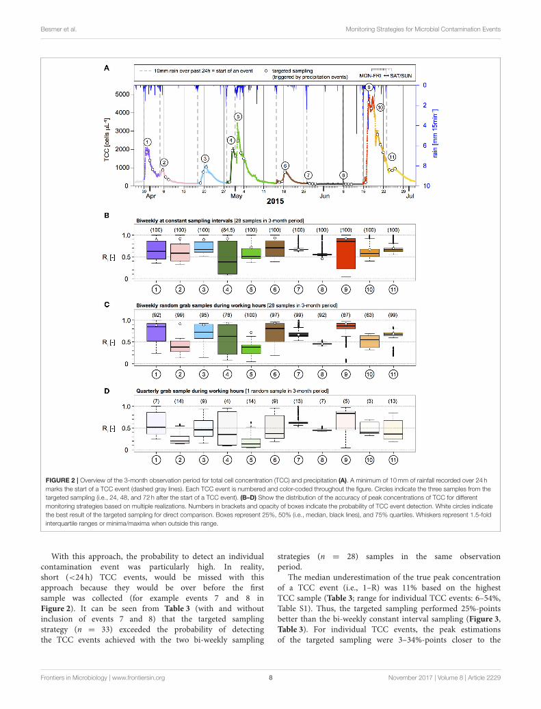
FIGURE 2 | Overview of the 3-month observation period for total cell concentration (TCC) and precipitation (A). A minimum of 10mm of rainfall recorded over 24 h
marks the start of a TCC event (dashed gray lines). Each TCC event is numbered and color-coded throughout the figure. Circles indicate the three samples from the
targeted sampling (i.e., 24, 48, and 72 h after the start of a TCC event). (B–D) Show the distribution of the accuracy of peak concentrations of TCC for different
monitoring strategies based on multiple realizations. Numbers in brackets and opacity of boxes indicate the probability of TCC event detection. White circles indicate
the best result of the targeted sampling for direct comparison. Boxes represent 25%, 50% (i.e., median, black lines), and 75% quartiles. Whiskers represent 1.5-fold
interquartile ranges or minima/maxima when outside this range.
With this approach, the probability to detect an individualcontamination event was particularly high. In reality,short (<24 h) TCC events, would be missed with thisapproach because they would be over before the firstsample was collected (for example events 7 and 8 inFigure 2). It can be seen from Table 3 (with and withoutinclusion of events 7 and 8) that the targeted samplingstrategy (n = 33) exceeded the probability of detectingthe TCC events achieved with the two bi-weekly sampling
strategies (n = 28) samples in the same observationperiod.
The median underestimation of the true peak concentrationof a TCC event (i.e., 1–R) was 11% based on the highestTCC sample (Table 3; range for individual TCC events: 6–54%,Table S1). Thus, the targeted sampling performed 25%-pointsbetter than the bi-weekly constant interval sampling (Figure 3,Table 3). For individual TCC events, the peak estimationsof the targeted sampling were 3–34%-points closer to the
Frontiers in Microbiology | www.frontiersin.org 8 November 2017 | Volume 8 | Article 2229

Besmer et al. Monitoring Strategies for Microbial Contamination Events
TABLE 3 | Overview of the different monitoring strategies and the resulting (1) probability to detect precipitation-induced TCC events and (2) accuracy of peak
concentration estimations of bacteria in karstic spring water during a 3-month observation period (Figure 2, Spring B).
Monitoring
strategy
Probability of TCC event detection Estimation of TCC peak concentration (R = sampled
maximum divided by true maximum)
n Average Range (%) Median (%)a 25% Quartile (%)a 75% Quartile (%)a Median range (%)b
Constant interval Quarterly 1 10 3–16 43 (31) 19 (17) 61 (59) 14–84
Monthly 3 29 10–48 44 (31) 19 (17) 62 (59) 14–84
Weekly 14 86 42–100 54 (47) 34 (29) 67 (68) 33–84
Bi-weekly 28 99 85–100 64 (64) 52 (49) 80 (84) 38–86
Daily 99 100 – 87 (89) 72 (82) 93 (93) 56–94
Randomly
(working hours)
Quarterly 1 9 2–15 41 (32) 20 (17) 62 (60) 16–83
Monthly 3 24 9–37 43 (36) 21 (18) 63 (64) 16–83
Weekly 14 71 35–91 51 (50) 32 (26) 68 (74) 23–85
Bi-weekly 28 91 63–100 61 (62) 41 (38) 84 (86) 38–87
Daily 70 100 – 81 (87) 55 (58) 92 (92) 46–93
Targeted 33 100 – 89 (90) 69 (72) 92 (92) 46–94
For the constant sampling interval and random sampling, multiple possible realizations were statistically summarized whereas for the targeted sampling only one realization exists in this
study. See Figure 3, Figures S2, S3 for graphical representations of the results and Table S1 for results of individual TCC events.aFor the combination of all realizations for all 11 TCC events in Figure 3 (in brackets without events 7 and 8).bFor the 11 individual TCC events; see Table S1 for all values.
0.0
0.2
0.4
0.6
0.8
1.0
quarterly
(1)
monthly
(3)
weekly
(14)
biweekly
(28)
event-based
(33)
daily
(99/70)
sampling interval
(number of samples in 3−month period)
ma
x(R
) [−
] fo
r a
ll eve
nts
for
all
rea
lisa
tio
ns
constant sampling
intervals (pre-defined)
random grab
samples during
working hours
targeted sampling
triggered by precipi-
tation events
FIGURE 3 | Comparison of estimation of peak concentration (R = sampled maximum divided by true maximum) for different monitoring strategies and number of
samples calculated for all realizations for all 11 TCC events (see Table 3 and Table S1 for detailed values). For the targeted sampling, the values were calculated for
one realization only for all 11 TCC events and the best R values (i.e., closest to the true value) out of three samples taken per TCC event were used. White lines
represent the median, boxes represent 25/75% quartiles, whiskers represent 1.5 times interquartile ranges (or minima/maxima). Horizontal dotted lines are 25%, 50%
(median), and 75% quartiles of the targeted sampling for comparison with other strategies and numbers of samples.
true values except for the minor events 7 and 8 (where thetargeted sampling performed equally well and 9%-points worserespectively) (Table S1). In addition, the targeted samplinghad much higher values and a narrower range for the 25and 75% quartiles, which the other monitoring strategieswould only reach with daily sampling (Figure 3, Table 3). Insummary, the targeted sampling achieved a moderately higherdetection probability of TCC events and a considerably better
estimation of peak concentrations with a similar number ofsamples.
In order to capture every single TCC event in our dataset, the targeted sampling strategy required 33 samples to betaken and analyzed (compared to 28 samples for a bi-weeklystrategy). However, the strength of the targeted sampling lies inthat it provides the utility with the choice to sample any givencontamination event with high accuracy, rather than necessarily
Frontiers in Microbiology | www.frontiersin.org 9 November 2017 | Volume 8 | Article 2229

Besmer et al. Monitoring Strategies for Microbial Contamination Events
trying to detect every TCC event. Also, it is evident that ifa system experiences fewer contamination events with longerperiods in between events than seen in the above example, thetargeted sampling will become considerably more efficient thanthe other two monitoring strategies.
Considerations on Generalization andSystem Specific CharacteristicsThe presented approach is considered to be generally validfor springs in geological settings and climatic regions that arefrequently influenced by precipitation-induced contaminationevents (Stadler et al., 2008; Butscher et al., 2011; Delbart et al.,2014; Meus et al., 2014; Sinreich et al., 2014). However, theconcepts discussed above are not limited to karstic springs,and can be developed for different systems (e.g., riverbankfiltration, surface waters, treatment plants). In this regard,targeted sampling strategies always need to be adapted tothe specific characteristics of the investigated system, and thefollowing aspects should be considered:
(1) The best variable to serve as the trigger for targeted samplingshould be identified based on an assessment of existingdata sets (e.g., precipitation data, operational data, onlinemeasurements of abiotic variables) and ideally also initialhigh-frequency microbial measurements (e.g., online flowcytometry or auto-sampler campaigns), if available.
(2) The threshold of the trigger variable that leads to the startof sampling is crucial for the detection probability of events.Too low thresholds lead to unnecessary high numbers ofsamplings of baseline conditions whereas too high thresholdsbare the risk of missing events. Initial high-frequencymicrobial measurements will support the identification ofsuch thresholds.
(3) The lag time between exceeding the trigger variable thresholdand first targeted sampling should be selected such thatthe latter ideally always occurs well before the peak ofthe contamination event. Again, the system-inherent lagtimes should ideally be extracted from initial high-frequencymicrobial measurements (see also Delbart et al., 2014).
(4) The sampling interval and the number of samples per eventshould be chosen such that the typical time scale of events inthe investigated system are adequately covered. This meansthat the contamination peak always falls into the sampledperiod and thus depends on lag time, sampling interval andnumber of samples.
Implications and PracticalRecommendationsThe suitability of TCC as a microbial process variable forimproved understanding of water resources shown previously(Vital et al., 2012; Gillespie et al., 2014; Helmi et al., 2014) wasextended to the investigation of short-term dynamics in thepresent study (Figure 1C). This highlights the value of measuringTCC (or similar cultivation-independent variables) automaticallyat high temporal resolution for microbial monitoring (Brognauxet al., 2013; Besmer et al., 2014; Besmer and Hammes, 2016).While TCC is not a direct hygienic indicator, it is one of the
most direct microbial variables that can be measured onlineand is seen as a useful process variable to detect microbialdynamics. Using online microbial measurements to drive atargeted sampling approach allows the use of more advancedmethods, e.g., for specific fecal indicator organisms or directpathogen and/or community detection, at meaningful pointsin time and comparison to long-term records (Figures 1B,E;Stadler et al., 2008; Goldscheider et al., 2010; Butscher et al.,2011).
While permanent online monitoring offers considerable
advantages (Janke et al., 2006) it will probably not bepractically and financially feasible for microbial water quality
monitoring in the near future – especially for smaller utilities.However, the two examples in our study clearly show thatafter initial high-frequency measurements during a limited
period, future targeted monitoring can be based on a moderatenumber of samples, which can be handled with an auto-sampler or even manual grab sampling and conventional
detection methods (e.g., indicator organisms). Our findingsclearly support the growing awareness that conventional waterquality monitoring approaches need to be improved to better
support risk assessment and system optimization (Petterson
and Ashbolt, 2016) and further confirm the high value ofautomated, targeted sampling to this end (Stadler et al.,2008).
Consequently, we propose the following practical
recommendations for improved monitoring of microbialshort-term dynamics in raw and treated drinking water
systems:
(1) Compile all available data and knowledge on possible
dynamics in water quality (e.g., precipitation data; onlinemeasurements of discharge, conductivity; conventionalmonitoring records).
(2) Prioritize systems or locations within a system (e.g., raw
water sources, treatment plants) with assumed or knownhigh variability in water quality based on the above data.
(3) Perform monitoring at the highest possible temporal
resolution for at least 10 events with available onlinetools for direct (e.g., TCC) or surrogate (e.g., turbidity,particle counter) detection of bacterial concentrations.
In natural systems, such as karstic springs, the possibleinfluence of seasonal differences should be taken intoaccount when performing high-frequency monitoringcampaigns.
(4) From the high-frequency data set, establish the causes andthe typical time scales of microbial dynamics.
(5) Specifically, identify the most suitable early-warning variable(e.g., precipitation event, increase in spring discharge,increase in turbidity) as a trigger for targeted sampling.
(6) Based on this compiled knowledge on the dynamics, testdifferent alternative monitoring strategies on the high-frequency data set as was demonstrated in this study.
(7) Implement the best alternative strategy that deliverssufficient information for the questions to be answered andis feasible with the resources available (see also: Ward et al.,1986; Harmel et al., 2006).
Frontiers in Microbiology | www.frontiersin.org 10 November 2017 | Volume 8 | Article 2229

Besmer et al. Monitoring Strategies for Microbial Contamination Events
CONCLUSIONS
• Bacterial concentrations in karstic spring water are usuallylow during dry weather periods but increase substantially afterlocalized precipitation events.
• Conventional monitoring strategies, which are based oninfrequent grab sampling, substantially underestimate boththe number of contamination events and peak concentrationsof bacteria during such contamination events.
• TCC is a useful measurement to track precipitation-inducedcontamination events in spring water.
• Emerging automated TCC measurement devices allow for thecollection of high-frequency data sets over extended periodsthat can be used for a systematic evaluation of short-termdynamics and monitoring strategies.
• Optimization of monitoring strategies should be site specificand based on (1) systematic analysis of existing data sets and(2) pilot studies with the highest possible temporal and spatialresolution and information depth to enable an informedoptimization of a targeted monitoring strategy.
• While higher sampling frequencies generally improve boththe probability of event detection and the estimation ofmicrobial peak concentrations, targeted sampling is mostefficient and effective and can be applied flexibly for individualcontamination events.
AUTHOR CONTRIBUTIONS
Experimental design: MB, JS, and FH. Research: MB, JS, and FH.Data analysis: MB, FH, and CO. Writing/editing: MB, JS, FH,and CO.
ACKNOWLEDGMENTS
The authors acknowledge the financial support from theCanton Basel-Landschaft, Switzerland in the framework ofthe project “Regionale Wasserversorgung Basel-Landschaft 21”as well as internal Eawag Discretionary Funding. We thankthe Food Safety and Veterinary Office Basel-Landschaft andTimon Langenegger for laboratory and field support, andthe local treatment plant operator and utility for theirforthcoming collaboration. The meteorological station wasoperated in cooperation with the group for Meteorology,Climatology, and Remote Sensing (MCR) at the University ofBasel.
SUPPLEMENTARY MATERIAL
The Supplementary Material for this article can be foundonline at: https://www.frontiersin.org/articles/10.3389/fmicb.2017.02229/full#supplementary-material
REFERENCES
Astrom, J., Petterson, S., Bergstedt, O., Pettersson, T. J. R., and Stenstrom, T. A.
(2007). Evaluation of the microbial risk reduction due to selective closure of
the raw water intake before drinking water treatment. J. Water Health 5, 81–97.
doi: 10.2166/wh.2007.139
Bakker, M., Vreeburg, J. H. G., Palmen, L. J., Sperber, V., Bakker, G., and Rietveld,
L. C. (2013). Better water quality and higher energy efficiency by using model
predictive flow control at water supply systems. J. Water Supply Res. Technol.
Aqua 62, 1–13. doi: 10.2166/aqua.2013.063
Besmer, M. D., and Hammes, F. (2016). Short-term microbial dynamics in a
drinking water plant treating groundwater with occasional high microbial
loads.Water Res. 107, 11–18. doi: 10.1016/j.watres.2016.10.041
Besmer, M. D., Epting, J., Page, R.M., Sigrist, J. A., Huggenberger, P., and Hammes,
F. (2016). Online flow cytometry reveals microbial dynamics influenced by
concurrent natural and operational events in groundwater used for drinking
water treatment. Sci. Rep. 6:38462. doi: 10.1038/srep38462
Besmer, M. D., Weissbrodt, D., G., Kratochvil, B., E., Sigrist, J., A., Weyland, M.,
S., and Hammes, F. (2014). The feasibility of automated online flow cytometry
for in-situ monitoring of microbial dynamics in aquatic ecosystems. Front.
Microbiol. 5:265. doi: 10.3389/fmicb.2014.00265
Brognaux, A., Han, S. S., Sorensen, S. J., Lebeau, F., Thonart, P., and Delvigne, F.
(2013). A low-cost, multiplexable, automated flow cytometry procedure for the
characterization of microbial stress dynamics in bioreactors. Microb. Cell Fact.
12:100. doi: 10.1186/1475-2859-12-100
Butscher, C., Auckenthaler, A., Scheidler, S., and Huggenberger, P. (2011).
Validation of a numerical indicator of microbial contamination for karst
springs. Ground Water 49, 66–76. doi: 10.1111/j.1745-6584.2010.00687.x
Casey, D., Nemetz, P. N., and Uyeno, D. H. (1983). Sampling frequency for
water-quality monitoring-measures of effectiveness. Water Resour. Res. 19,
1107–1110. doi: 10.1029/WR019i005p01107
Delbart, C., Valdes, D., Barbecot, F., Tognelli, A., Richon, P., and Couchoux,
L. (2014). Temporal variability of karst aquifer response time established
by the sliding-windows cross-correlation method. J. Hydrol. 511, 580–588.
doi: 10.1016/j.jhydrol.2014.02.008
Do, H. T., Lo, S. L., and Lan, A. P. T. (2013). Calculating of river
water quality sampling frequency by the analytic hierarchy process
(AHP). Environ. Monit. Assess. 185, 909–916. doi: 10.1007/s10661-012-
2600-6
Farnleitner, A. H., Wilhartitz, I., Ryzinska, G., Kirschner, A. K. T., Stadler,
H., Mach, R. L. et al. (2005). Bacterial dynamics in spring water of
alpine karst aquifers indicates the presence of stable autochthonous
microbial endokarst communities. Environ. Microbiol. 7, 1248–1259.
doi: 10.1111/j.1462-2920.2005.00810.x
Field, M. S., and Nash, S. G. (1997). Risk assessment methodology for karst
aquifers: (1) Estimating karst conduit-flow parameters. Environ. Monit. Assess.
47, 1–21.
Gauthier, V., Barbeau, B., Millette, R., Block, J.-C., and Prévost, M. (2001).
Suspended particles in the drinking water of two distribution systems. Water
Sci. Technol. 1, 237–245. Available online at: http://ws.iwaponline.com/content/
1/4/237
Gillespie, S., Lipphaus, P., Green, J., Parsons, S., Weir, P., Juskowiak, K., et al.
(2014). Assessing microbiological water quality in drinking water distribution
systems with disinfectant residual using flow cytometry. Water Res. 65,
224–234. doi: 10.1016/j.watres.2014.07.029
Goldscheider, N., Pronk, M., and Zopfi, J. (2010). New insights into the transport
of sediments and microorganisms in karst groundwater by continuous
monitoring of particle-size distribution. Geologia Croatica 63, 137–142.
doi: 10.4154/gc.2010.10
Harmel, R. D., King, K. W., Haggard, B. E., Wren, D. G., and Sheridan,
J., M. (2006). Practical guidance for discharge and water quality data
collection on small watersheds. Trans. Asabe 49, 937–948. doi: 10.13031/2013.
21745
Helmi, K., Watt, A., Jacob, P. I., Ben-Hadj-Salah, Henry, A., Meheut, G.,
Charni-Ben-Tabassi, N., et al. (2014). Monitoring of three drinking water
treatment plants using flow cytometry. Water Sci. Technol. 14, 850–856.
doi: 10.2166/ws.2014.044
Hojris, B., Christensen, S. C. B., Albrechtsen, H. J., Smith, C., and Dahlqvist, M.
(2016). A novel, optical, on-line bacteria sensor for monitoring drinking water
quality. Sci. Rep. 6: 23935. doi: 10.1038/srep23935
Frontiers in Microbiology | www.frontiersin.org 11 November 2017 | Volume 8 | Article 2229

Besmer et al. Monitoring Strategies for Microbial Contamination Events
ISO (2000). Detection and Enumeration of Escherichia Coli and Coliform Bacteria-
Part 1: Membrane Filtration Method. Geneva: ISO. 9308-1:2000.
ISO (2003). Horizontal Method for the Enumeration of Microorganisms-Colony-
Count Technique at 30 Degrees. Geneva: ISO. 4833:2003.
ISO (2005). General Requirements for the Competence of Testing and Calibration
Laboratories. Geneva: ISO. 17025:2005.
ISO (2006). Sampling-part 1: Guidance on the Design of Sampling Programmes and
Sampling Techniques. Geneva: ISO. 5667-1:2006.
ISO (2012). Conformity Assessment-Requirements for the Operation of Various
Types of Bodies Performing Inspection. Geneva: ISO. 17020:2012.
Janke, R., Murray, R., Uber, J., and Taxon, T. (2006). Comparison of physical
sampling and real-time monitoring strategies for designing a contamination
warning system in a drinking water distribution system. J. Water Resour. Plan.
Manage. 132, 310–313. doi: 10.1061/(ASCE)0733-9496(2006)132:4(310)
Kistemann, T., Classen, T., Koch, C., Dangendorf, F., Fischeder, R., Gebel,
J., et al. (2002). Microbial load of drinking water reservoir tributaries
during extreme rainfall and runoff. Appl. Environ. Microbiol. 68, 2188–2197.
doi: 10.1128/AEM.68.5.2188-2197.2002
Liu, Y., Zheng, B. H., Wang, M., Xu, Y. X., and Qin, Y. W. (2014). Optimization
of sampling frequency for routine river water quality monitoring. Sci China 57,
772–778. doi: 10.1007/s11426-013-4968-8
Loftis, J. C., and Ward, R. C. (1980). Water-quality monitoring-some
practical sampling frequency considerations. Environ. Manage. 4, 521–526.
doi: 10.1007/BF01876889
Madrid, Y., and Zayas, Z. P. (2007). Water sampling: traditional methods and new
approaches in water sampling strategy. Trac Trends Analyt. Chem. 26, 293–299.
doi: 10.1016/j.trac.2007.01.002
Meus, P., Moureaux, P., Gailliez, S., Flament, J., Delloye, F., and Nix, P. (2014).
In situ monitoring of karst springs in Wallonia (southern Belgium). Environ.
Earth Sci. 71, 533–541. doi: 10.1007/s12665-013-2760-x
Naddeo, V., Scannapieco, D., Zarra, T., and Belgiorno, V. (2013). River
water quality assessment: implementation of non-parametric tests
for sampling frequency optimization. Land Use Policy 30, 197–205.
doi: 10.1016/j.landusepol.2012.03.013
Page, R. M., Besmer, M. D., Epting, J., Sigrist, J. A., Hammes, F., and Huggenberger,
P. (2017). Online analysis: deeper insights into water quality dynamics in spring
water. Sci. Total Environ. 599, 227–236. doi: 10.1016/j.scitotenv.2017.04.204
Petterson, S. R., and Ashbolt, N. J. (2016). QMRA and water safety management:
review of application in drinking water systems. J. Water Health 14, 571–589.
doi: 10.2166/wh.2016.262
Prest, E. I., Hammes, F., Kotzsch, S., van Loosdrecht,M. C.M., andVrouwenvelder,
J. S. (2013). Monitoring microbiological changes in drinking water systems
using a fast and reproducible flow cytometric method. Water Res. 47,
7131–7142. doi: 10.1016/j.watres.2013.07.051
Pronk, M., Goldscheider, N., and Zopfi, J. (2006). Dynamics and interaction of
organic carbon, turbidity and bacteria in a karst aquifer system. Hydrogeol. J.
14, 473–484. doi: 10.1007/s10040-005-0454-5
Pronk, M., Goldscheider, N., and Zopfi, J. (2007). Particle-size distribution as
indicator for fecal bacteria contamination of drinking water from karst springs.
Environ. Sci. Technol. 41, 8400–8405. doi: 10.1021/es071976f
R Development Core Team (2008). R: A Language and Environment for Statistical
Computing. Vienna: R Foundation for Statistical Computin. Available online at:
http://cran.r-project.org/
Ryzinska-Paier, G., Lendenfeld, T., Correa, K., Stadler, P., Blaschke, A. P.,
Farnleitner, A. H., et al. (2014). A sensitive and robust method for automated
on-line monitoring of enzymatic activities in water and water resources.Water
Sci. Technol. 69, 1349–1358. doi: 10.2166/wst.2014.032
Scheidleder, A. (1999).Groundwater Quality and Quantity in Europe. Copenhagen:
European Environment Agency.
Signor, R. S., and Ashbolt, N. J. (2006). Pathogen monitoring offers
questionable protection against drinking-water risks: a QMRA
(Quantitative Microbial Risk Analysis) approach to assess management
strategies. Water Sci. Technol. 54, 261–268. doi: 10.2166/wst.20
06.478
Sinreich, M., Pronk, M., and Kozel, R. (2014). Microbiological monitoring
and classification of karst springs. Environ. Earth Sci. 71, 563–572.
doi: 10.1007/s12665-013-2508-7
Skeffington, R. A., Halliday, S. J., Wade, A. J., Bowes, M. J., and Loewenthal, M.
(2015). Using high-frequency water quality data to assess sampling strategies
for the EUWater Framework Directive. Hydrol. Earth Syst. Sci. 19, 2491–2504.
doi: 10.5194/hess-19-2491-2015
SLMB (2007). Method 1406.1: Detection of Enterococcus spp. (Schweizerisches
Lebensmittelhandbuch). Berne: Federal Office for Public Health.
SLMB (2012). Method 333.1: Determining the Total Cell Count And Ratios Of
High And Low Nucleic Acid Content Cells in Freshwater Using Flow Cytometry.
(Schweizerisches Lebensmittelhandbuch). Berne: Federal Office for Public
Health.
Stadler, H., Skritek, P., Sommer, R., Mach, R. L., Zerobin, W., and Farnleitner,
A. H. (2008). Microbiological monitoring and automated event sampling
at karst springs using LEO-satellites. Water Sci. Technol. 58, 899–909.
doi: 10.2166/wst.2008.442
Stevenson, D. G. (1997). Water Treatment Unit Processes. London: Imperial
College Press.
Storey, M. V. van der Gaag, B., and Burns, B. P. (2011). Advances in on-line
drinking water quality monitoring and early warning systems. Water Res. 45,
741–747. doi: 10.1016/j.watres.2010.08.049
Vital, M., Dignum, M., Magic-Knezeu, A., Ross, P., Rietueld, L., and
Hammes, F. (2012). Flow cytometry and adenosine tri-phosphate analysis:
alternative possibilities to evaluate major bacteriological changes in drinking
water treatment and distribution systems. Water Res. 46, 4665–4676.
doi: 10.1016/j.watres.2012.06.010
Vreeburg, J. H. G., Schaap, P. G., and van Dijk, J. C. (2004). “Particles in
the drinking water system: from source to discolouration,” in 4th World
Water Congress: Innovation in Drinking Water Treatment, Vol. 4 (Marrakesh;
London), 431–438.
Ward, R. C., Loftis, J. C., andMcbride, G. B. (1986). The data-rich but information-
poor syndrome in water-quality monitoring. Environ. Manage. 10, 291–297.
Conflict of Interest Statement: The authors declare that the research was
conducted in the absence of any commercial or financial relationships that could
be construed as a potential conflict of interest.
The reviewer PS and handling Editor declared their shared affiliation.
Copyright © 2017 Besmer, Hammes, Sigrist and Ort. This is an open-access article
distributed under the terms of the Creative Commons Attribution License (CC BY).
The use, distribution or reproduction in other forums is permitted, provided the
original author(s) or licensor are credited and that the original publication in this
journal is cited, in accordance with accepted academic practice. No use, distribution
or reproduction is permitted which does not comply with these terms.
Frontiers in Microbiology | www.frontiersin.org 12 November 2017 | Volume 8 | Article 2229