evaluating equivalence testing methods for …
TRANSCRIPT

EVALUATING EQUIVALENCE TESTING METHODS FOR MEASUREMENT INVARIANCE
ALYSSA COUNSELL
A DISSERTATION SUBMITTED TO THE FACULTY OF GRADUATE STUDENTS IN PARTIAL FULFILLMENT OF THE REQUIREMENTS FOR
THE DEGREE OF DOCTOR OF PHILOSOPHY
GRADUATE PROGRAM IN PSYCHOLOGY YORK UNIVERSITY
TORONTO, ON
AUGUST 2017
© ALYSSA COUNSELL, 2017

ii
ABSTRACT
Establishing measurement invariance (MI) is important to validly make group
comparisons on psychological constructs of interest. MI involves a multi-stage process of
determining whether the factor structure and model parameters are similar across
multiple groups. The statistical methods used by most researchers for testing MI is by
conducting multiple group confirmatory factor analysis models, whereby a statistically
nonsignificant results in a 𝜒! difference test or a small change in goodness of fit indices
(∆GOFs) such as CFI or RMSEA are used to conclude invariance. Yuan and Chan (2016)
proposed replacing these approaches with an equivalence test analogue of the 𝜒!
difference test (EQ). While they outline the EQ approach for MI, they recommend using
an adjusted RMSEA version (EQ-A) for increased power. The current study evaluated
the Type I error and power rates of the EQ and EQ-A and compare their performance to
using traditional 𝜒! difference tests and ∆GOFs. Results demonstrate that the EQ for
nested models was the only procedure that maintains empirical error rates below the
nominal level. Results also highlight that the EQ requires larger sample sizes or
equivalence bounds based on larger than conventional RMSEA values like .05 to ensure
adequate power rates at later MI stages. Because the EQ-A test did not maintain accurate
error rates, I do not recommend Yuan and Chan’s proposed adjustment.

iii
ACKNOWLEDGEMENTS First and foremost I would like to acknowledge the hard work and dedication of
my supervisor and mentor, Rob Cribbie. Rob has been an outstanding supervisor and the
level of support that he provided, be it academic, financial or emotional, was above and
beyond what any student could ever expect. I can say without reservation that I am where
I am today because of Rob. Thank you Rob for pushing me to be the best researcher,
writer, and teacher that I could be.
Next, I would like to thank Dave Flora, who contributed the most insight and
expertise to this project. Each time (and there were many!) that I asked Dave for his
thoughts and advice, I gained a better understanding of my research topic as well as
tangential issues of interest. Dave’s comments on early drafts vastly improved my paper.
He also deserves credit for inspiring my dissertation topic because it was his
psychometrics course where I became interested in measurement invariance and started
thinking about how it could be incorporated into equivalence testing.
I would also like to acknowledge the contributions of my committee members
who each provided a unique perspective that ultimately improved my dissertation. John
Eastwood continued to push the way I thought about larger theoretical issues and
constructs involved in SEM, and how the tools presented in my work reconcile (or fail to
reconcile) them. Raymond Mar’s feedback ensured that my work was understandable to
both methodologists and applied researchers alike. Furthermore, in my first year as a
graduate student, I took a course with Raymond that helped shape my academic writing,
and I cannot thank him enough for the resources and recommendations that he provided.

iv
Georges Monette continually expanded the way I thought about statistical and
mathematical constructs. I have learned a lot from Georges by listening to his thoughts
during my time at the statistical consulting service. Dennis Jackson provided excellent
feedback and questions that I had not previously considered. I also used Dennis’ work to
help provide rationale for some of the simulation conditions and decisions made in
setting up my study. A big thank you to each of my committee members for their
engagement and enthusiasm for this project.
I must acknowledge the emotional support of a number of individuals who helped
keep me sane enough to finish my degree. Kristen Maki, Heather Davidson, Joana Katter,
Taryn Nepon, Saeid Chavoshi, Wendy Zhao, and Whitney Taylor all provided support
and encouragement at crucial stages throughout my degree. I would like to further thank
Kristen, Heather, Joana, and Saeid as well as Nataly Beribisky and Linda Farmus for
attending my oral examination.
I would also like to thank my partner, Ye Tian for his unwavering support over
the years. Despite many ups and downs and crazy hours, Ye has helped push me to finish
my degree in a timely manner while simultaneously providing unconditional support and
encouragement. Lastly, I would like to acknowledge my pup and writing buddy, Nacho,
who kept me company during the many hours spent in front of my computer writing this
document. This fur ball made the solitary act of writing just a little less lonely.

v
Table of Contents
Abstract .............................................................................................................................. ii Acknowledgements ............................................................................................................ iii Table of Contents ................................................................................................................ v List of Tables .................................................................................................................... vii List of Figures ..................................................................................................................... x
Chapter One: Introduction .................................................................................................. 1 Confirmatory Factor Analysis ......................................................................................... 2 Assessing Model Fit ........................................................................................................ 3
Comparative Fit Index ................................................................................................ 5 McDonald’s Noncentrality Index ............................................................................... 6 Root Mean Square Error of Approximation ............................................................... 6
Testing Measurement Invariance with Multiple Group CFA ......................................... 8 Configural Invariance ................................................................................................. 9 Metric Invariance ........................................................................................................ 9 Scalar Invariance ....................................................................................................... 10 Strict Invariance ........................................................................................................ 10 Model Comparison with χ2 Difference Tests ........................................................... 11 Model Comparison through Change in Goodness of Fit .......................................... 12
Chapter Two: Applying Equivalence Testing to Measurement Invariance ...................... 15 Equivalence Testing ...................................................................................................... 15 Equivalence Intervals .................................................................................................... 16 Equivalence Testing Methods for Measurement Invariance ........................................ 17
TML equivalence test .................................................................................................. 17 Equivalence testing alternative to the χ2 difference test .......................................... 18 What is an appropriate equivalence interval? ........................................................... 19 The Test of Close Fit ................................................................................................. 21
Chapter Three: Method and Results ................................................................................. 23 Method .......................................................................................................................... 23
Power Conditions ...................................................................................................... 26 Type I Error Conditions ............................................................................................ 27
Results ........................................................................................................................... 31 Nonconvergence ....................................................................................................... 31 Empirical Type I error rates ...................................................................................... 31 Empirical Power Rates .............................................................................................. 38
Chapter Four: Empirical Example .................................................................................... 43 Results Using the Traditional Methods for MI ............................................................. 44 Results Using the Equivalence Testing Methods for MI .............................................. 46 Results Using the GOF Indices ..................................................................................... 47 Implications for Substantive Conclusions .................................................................... 48
vi
Chapter Five: Discussion .................................................................................................. 50 Equivalence Tests Versus Difference-based Tests ....................................................... 50 Performance of the Equivalence Tests for MI .............................................................. 51 Using Change in Goodness of Fit Indices ..................................................................... 52 Choosing an Equivalence Interval ................................................................................ 53 Tests of Global Fit vs. Local Fit ................................................................................... 55 Practicalities of Measurement Invariance Testing ........................................................ 56 Limitations and Future Directions ................................................................................ 58 Conclusion .................................................................................................................... 60
References ......................................................................................................................... 62
Tables ................................................................................................................................ 73 Figures............................................................................................................................. 161

vii
LIST OF TABLES
Table 1: Population Model Parameters for Second Power Condition 73
Table 2: Population Model Parameters for Type I Error Conditions 74
Table 3: Type I Error Rates for Group 1 Model Fit (4 indicator model) 75
Table 4: Type I Error Rates for Group 2 Model Fit (4 indicator model) 77
Table 5: Type I Error Rates for Group 1 Model Fit (8 indicator model) 79
Table 6: Type I Error Rates for Group 2 Model Fit (8 indicator model) 81
Table 7 Type I Error Rates for Configural Invariance (4 indicator model) 83
Table 8 Type I Error Rates for Configural Invariance (8 indicator model) 85
Table 9 Type I Error Rates for Metric Invariance (4 indicator model, Single
noninvariant loading)
87
Table 10 Type I Error Rates for Metric Invariance (8 indicator model, Single
noninvariant loading)
89
Table 11 Type I Error Rates for Metric Invariance (4 indicator model, 25%
noninvariant loadings)
91
Table 12 Type I Error Rates for Metric Invariance (8 indicator model, 25%
noninvariant loadings)
93
Table 13 Type I Error Rates for Scalar Invariance (4 indicator model, Single
noninvariant intercept)
95
Table 14 Type I Error Rates for Scalar Invariance (8 indicator model, Single
noninvariant intercept)
97
Table 15 Type I Error Rates for Scalar Invariance (4 indicator model, 25%
noninvariant intercepts)
99
Table 16 Type I Error Rates for Scalar Invariance (8 indicator model, 25%
noninvariant intercepts)
101
Table 17 Type I Error Rates for Strict Invariance (4 indicator model, Single
noninvariant variance)
103

viii
Table 18 Type I Error Rates for Strict Invariance (8 indicator model, Single
noninvariant variance)
105
Table 19 Type I Error Rates for Strict Invariance (4 indicator model, 25%
noninvariant variances)
107
Table 20 Type I Error Rates for Strict Invariance (8 indicator model, 25%
noninvariant variances)
109
Table 21 Power for Group 1 Model Fit (4 indicator model) with No Model
Misspecification
111
Table 22 Power for Group 2 Model Fit (4 indicator model) with No Model
Misspecification
113
Table 23 Power for Group 1 Model Fit (8 indicator model) with No Model
Misspecification
115
Table 24 Power for Group 2 Model Fit (8 indicator model) with No Model
Misspecification
117
Table 25 Power Rates for Configural Invariance (4 indicator model) with no
Model Misspecification
119
Table 26 Power Rates for Configural Invariance (8 indicator model) with no
Model Misspecification
121
Table 27 Power for Group 1 Model Fit (4 indicator model) with Small degree
of Model Misspecification
123
Table 28 Power for Group 2 Model Fit (4 indicator model) with Small degree
of Model Misspecification
125
Table 29 Power for Group 1 Model Fit (8 indicator model) with Small degree
of Model Misspecification
127
Table 30 Power for Group 2 Model Fit (8 indicator model) with Small degree
of Model Misspecification
129
Table 31 Power Rates for Configural Invariance (4 indicator model with small
degree of model misspecification)
131

ix
Table 32 Power Rates for Configural Invariance (8 indicator model with small
degree of model misspecification)
133
Table 33 Power Rates for Metric Invariance (4 indicator identical group
population models)
135
Table 34 Power Rates for Metric Invariance (8 indicator identical group
population models)
137
Table 35 Power Rates for Metric Invariance (4 indicator population models
with small group difference in single loading)
139
Table 36 Power Rates for Metric Invariance (8 indicator population models
with small group difference in single loading)
141
Table 37 Power Rates for Scalar Invariance (4 indicator identical group
population models)
143
Table 38 Power Rates for Scalar Invariance (8 indicator identical group
population models)
145
Table 39 Power Rates for Scalar Invariance (4 indicator population models
with small group difference in single intercept)
147
Table 40 Power Rates for Scalar Invariance (8 indicator population models
with small group difference in single intercept)
149
Table 41 Power Rates for Strict Invariance (4 indicator identical group
population models)
151
Table 42 Power Rates for Strict Invariance (8 indicator identical group
population models)
153
Table 43 Power Rates for Strict Invariance (4 indicator population models with
small group difference in single variance)
155
Table 44 Power Rates for Strict Invariance (8 indicator population models with
small group difference in single variance)
157
Table 45 Estimates from single group male model in data example 159
Table 46 Estimates from single group female model in data example 160

x
LIST OF FIGURES Figure 1 Path diagrams for each of the measurement models used in simulation 161
Figure 2 Rates of falsely concluding equivalence for model fit in a single
group when RMSEA0 = .08 and factor loadings are .7
162
Figure 3 Rates of falsely concluding equivalence for metric invariance in the 4
indicator model when RMSEA0 = .08
163
Figure 4 Rates of correctly concluding invariance (power rates for the EQ) 164
Figure 5 Measurement model for the five-factor Generic Conspiracist Beliefs
Scale (GCB) used in the applied data example
165

1
CHAPTER ONE
INTRODUCTION
Many constructs in psychology cannot be measured directly; instead they are
approximated by tests and surveys, which necessarily result in some degree of
measurement error. Measurement error has implications for examining construct
differences between populations because researchers want to ensure that any differences
are a function of group membership and not confounded with measurement error or bias.
One way to distinguish between true group differences and measurement error is by
testing measurement invariance (MI). Tools that allow researchers to test their
instruments, scales, and composite measures for MI allow for more reliable measurement
of psychological phenomena and more accurate portrayals of psychological constructs
across different groups. Examples include demonstrating that scales are invariant for
different ethnic or cultural groups, for scales that have been translated into different
languages, or for groups that might differ based on other demographic variables such as
age or gender. A recent example includes the work of Belon and colleagues (2015) who
sought to establish MI on the Eating Disorders Inventory for Hispanic and white females.
Using confirmatory factor analysis (CFA) models, they found that the same three-factor
structure was present in both white and Hispanic participants, but factor loadings were
non-invariant across the two groups.
Much of the work in MI has focused on tests designed to detect differences
between measurement model parameters. Using methods designed for detecting

2
differences presents a challenge for MI when the researcher’s goal is to determine that
there are similarities across group parameters. Equivalence testing is an area of research
that originated in pharmacokinetics, where researchers had goals to statistically support
evidence of equivalence or similarity (e.g., similar effects of brand name and generic
drugs). While less popular in psychology, I will argue that the field of equivalence testing
is not only relevant for MI, but more appropriately aligned with its purpose. Equivalence
testing and its applications will be discussed in more detail in subsequent sections. The
purpose of this project is to evaluate and improve upon the equivalence testing procedure
for MI outlined by Yuan and Chan (2016). First, this paper introduces MI, its statistical
tool of confirmatory factor analysis, and shortcomings of the current techniques for
testing MI. The next section introduces equivalence testing generally and discusses its
application to MI and the tests described in Yuan and Chan’s work. Part III discusses the
methodology and results of a simulation study evaluating the performance (i.e., Type I
errors and power) of Yuan and Chan’s test. Finally, I discuss the numerical and
theoretical differences between traditional methods and equivalence testing methods for
testing MI, provide an illustration of the different approaches using real data, and provide
conclusions and recommendations.
Confirmatory Factor Analysis
CFA models latent variables or factors by testing a hypothesized factor structure
underlying a set of observed variables, taking into account measurement error (Bollen,
1989). The relationship between the observed variables and the factors can be represented
by the following equation:

3
𝒙 = 𝛖! + 𝚲!𝝃+ 𝜹 1
x is the vector of the p observed variables, 𝛖! is the p x 1 vector of intercepts, 𝚲𝒙 is a p x
r matrix of the factor loadings, where r is the number of latent variables or factors
contained in the r x 1 vector 𝝃, and 𝜹 is the p x 1 vector containing the measurement error
(the part of x not explained by the latent variables). Equation 1 states that the observed
variables are a function of underlying latent variables and measurement error. Examining
the plausibility of one’s hypothesized factor structure involves testing whether the
estimated covariance matrix S is equal to a model-implied covariance matrix 𝚺(𝛉) and
whether the estimated mean vector 𝒙 is equal to the model-implied mean structure 𝝁𝒌.
The model-implied covariance matrix and mean structure are:
𝚺 𝛉 = 𝚲𝒙𝚽𝚲!𝒙 + 𝚯𝜹, 𝝁𝒙 = 𝝉𝒙 + 𝚲𝒙𝜿 (2)
where 𝚲𝒙 is the factor loading matrix described above, 𝚽 is the model implied r x r
covariance matrix for the factors, 𝚯𝜹 is the model implied p x p covariance matrix for the
error terms in δ , 𝝁𝒙 is the p x 1 model-implied mean vector for the observed variables,
𝝉𝒙 is the p x 1 vector of intercepts, and 𝜿 is the r x 1 vector of factor means. The null
hypothesis for a single-group CFA is that the population covariance matrix is equal to the
model implied covariance matrix; that is, 𝐻!: 𝚺 = 𝚺(𝛉) (Bollen, 1989).
Assessing Model Fit
Since researchers can never know whether their model has correctly specified
parameters, the free parameters in 𝚺(𝛉) must be estimated from the sample covariance
matrix, S. In order to test the plausibility of one’s CFA model, the model implied matrix

4
with parameter estimates 𝚺 is compared to S through an estimator that seeks to minimize
the discrepancy between them. The most common estimator is maximum likelihood
(ML), which is implemented using the fitting function
𝐹!" = 𝒙− 𝝁 !𝚺 –𝟏 𝒙− 𝝁 + 𝑡𝑟 𝑺𝚺 !𝟏 − log 𝑺𝚺 !𝟏 − 𝑝 3
where 𝒙 and 𝝁 are the sample and model-implied mean vectors, respectively, and p is the
number of observed variables. Model fit can then be evaluated by a likelihood ratio test
based on:
𝑇!" = 𝑁 − 1 𝐹!" (4)
where N is the sample size and 𝑇!" is distributed as 𝜒!"! with degrees of freedom (df)
equal to the total number of non-redundant elements in S and 𝒙 minus the number of free
parameters. Note that because 𝑇!" is distributed as 𝜒!, it is sometimes simply referred to
as the 𝜒! statistic. When using 𝑇!" to assess model fit, the goal is to find a test statistic
that is not statistically significant, i.e., p > α, because the null hypothesis is that the model
implied covariance matrix perfectly matches the population covariance matrix. A number
of researchers have discussed that using the 𝑇!" alone as an index for model fit is
problematic (e.g., Bentler, 1990; Browne & Cudeck, 1992; Chen, 2007; Cheung &
Rensvold, 2002; Kang, McNeish, & Hancock, 2016; MacCallum, Browne, & Sugawara,
1996; Moshagen & Erdfelder, 2016). The two main arguments against using it are: i) its
sensitivity to sample size; and ii) that a test against perfect model fit is not realistic in
practice because models are only ever an approximation to reality. Therefore, a number
of alternative model fit indices have been proposed. In practice, 𝑇!" is still reported, but

5
researchers rely more heavily on other fit indices (Jackson, Gillaspy, & Purc-Stephenson,
2009; McDonald & Ringo Ho, 2002).
Although there are a large number of alternative fit indices, I will focus on three:
the comparative fit index (CFI, Bentler, 1990), the root mean square error of
approximation (RMSEA, Steiger, 1989), and McDonald’s noncentrality index (MNCI;
McDonald, 1989). The CFI and RMSEA were chosen because they are the most
commonly reported fit indices in applied research (Jackson et al., 2009), due in part to
their good statistical properties. The MNCI was included because research suggests that it
performs well for comparing models within the context of MI testing (Cheung &
Rensvold, 2002; Kang et al., 2016; Meade, Johnson, & Braddy, 2008). The use of MNCI
will be discussed in more detail in the sections comparing models for MI.
Comparative Fit Index
The CFI was proposed by Bentler (1990). It measures the relative improvement in
model fit of the researcher’s model compared to a baseline model:
𝐶𝐹𝐼 = 1−𝜒!! − 𝑑𝑓! 𝜒!! − 𝑑𝑓!
, (5)
where the subscript M indexes the researcher’s model and the subscript B refers to the
baseline model. The baseline model is typically the independence model, which assumes
no correlation between the measured variables. CFI values closer to 1 indicate better
model fit. An earlier convention was that values greater than .90 are considered indicative
of a good fitting model, but this guideline had little empirical justification. After the work
of Hu and Bentler (1999), values over .95 are advocated instead (Kline, 2015). One

6
potential benefit of the CFI is that it has been found to be relatively uninfluenced by
sample size (Fan, Thompson, & Wang, 1999; Sivo, Fan, Witta, & Willse, 2006). A
potential limitation, however, is the utility of using the independence model as the
comparison value since it is unlikely that the observed variables have zero correlation
with one another (Kline, 2015; Widaman & Thompson, 2003). Nevertheless, the
independence model remains popular for its theoretical importance.
McDonald’s Noncentrality Index
Like the CFI, the MNCI provides a measure of goodness of fit:
𝑀𝑁𝐶𝐼 = exp !!!
𝜒!! − 𝑑𝑓!𝑁 − 1 (7)
where values closer to 1 indicate better model fit. Based on the work of Hu and Bentler
(1999), .95 is recommended as the threshold for considering a model to have good fit.
The MNCI is rarely used in practice as a measure of overall model fit (Jackson et al.,
2009). Instead, much of the research evaluating its utility is for the purpose of MI testing,
which will be described in a later section.
Root Mean Square Error of Approximation
While the CFI and MNCI provide information about how well the model fits, the
RMSEA can be considered an index of how poorly the model fits; it is based on an
approximation of errors. The RMSEA is based on a noncentrality parameter that shifts
the 𝜒! distribution by its df:

7
𝑅𝑀𝑆𝐸𝐴 = 𝜒!! − 𝑑𝑓! 𝑑𝑓!(𝑁 − 1)
. (6)
If 𝜒!! < 𝑑𝑓!, the RMSEA is set to 0. Values closer to 0 indicate better model fit.
Recommendations vary for RMSEA but generally values less than .05 or .06 are
indicative of a good fitting model, and less than .07 or .08 is considered adequate model
fit (Hu & Bentler, 1999; Kline, 2015; Steiger, 2007). MacCallum and colleagues (1996)
proposed a range of values such that .01, .05, .08, and .10 could be considered excellent,
good, mediocre, and poor fit respectively.
The RMSEA favours parsimony such that, holding all else constant, it will favour
models with a smaller number of free parameters (Kline, 2015; Sivo et al., 2006). While
some may consider inflated RMSEA values at smaller sample sizes and low df models
problematic, others note that this is not actually a problem, and is in fact, statistically
appropriate (e.g., Cudeck & Henly, 1991; Sivo et al., 2006).
Despite the large number of fit indices developed to reconcile issues with using
the 𝑇!" statistic alone, they are not without limitations. One limitation is that because fit
indices measure model fit typically for large hypothesized models, they may indicate
good fit even when specific components of the model actually fit poorly (Reisinger &
Mavondo, 2006; Tomarken & Waller, 2003). Yuan (2005) notes that there is no specific
null hypothesis associated with fit indices and therefore cut-offs for fit indices cannot be
used like a traditional critical value in hypothesis testing. This criticism does not truly
apply to all fit indices, though, as one can use a null hypothesis with RMSEA
(MacCallum et al., 1996) and software commonly reports a test of a null hypothesis that

8
RMSEA < .05. Yuan (2005) further discusses how many fit indices do not have known
distributions when there is no model misspecification, thus it is difficult to determine
their sensitivity to model misspecification under a variety of other conditions. Due to
these pitfalls, Barrett (2007) advocates eliminating the use of fit indices altogether. This
is an extreme stance, with most researchers taking a more moderate stance of
recommending caution for interpreting fit indices, particularly avoidance of strict
adherence to recommended cut-offs (e.g., Marsh, Hau, & Wen, 2004; Steiger, 2007).
Testing Measurement Invariance with Multiple Group CFA
When a factor structure for a scale has been established, the next step is to ensure
that the scale does not function differently for different groups (i.e., there is no
measurement bias depending on group membership). This can be accomplished by
incorporating multiple groups into a CFA model to examine potential differences in the
model parameters by group. In a multi-group CFA, the null hypothesis becomes
𝐻!: 𝚺(𝟏) = 𝚺(𝟐) = . . .= 𝚺(𝑲), and 𝑇!" can easily be extended to the multi-group case:
𝑇!" = 𝑁 − 𝐾 𝐹!" = (𝑁! − 1)𝐹!"! + (𝑁! − 1)𝐹!"
! +⋯+ (𝑁! − 1)𝐹!"! (8)
for K groups, where N1, N2, NK are the sample sizes in the indexed group.
Using a series of nested models with increasing model constraints, researchers can
test various levels of MI such as the equality of the loadings, intercepts, and error
variances across the groups. Given the importance of constraints, the less stringent levels
of MI must precede the more stringent in a stepwise manner to ensure that equality
constraints on parameters are appropriate (Byrne, Shavelson, & Muthén, 1989; Millsap,
2011; Reise, Widaman, & Pugh, 1993; Vandenberg & Lance, 2000).

9
Despite common convention, the decision to test loadings before intercepts is somewhat
arbitrary, and recent research has advocated reversing the order of testing these
constraints when using categorical indicators (Wu & Estabrook, 2016). With categorical
variables, the method of identifying the latent variables will have implications for the
scale of the thresholds; however, this issue does not arise with continuous indicators
because the observed variables have an inherent scale based on their means and
variances. Since this study uses continuous indicators, I will follow the MI sequence
outlined below.
Configural Invariance
As a first step, a researcher must establish that the overall factor structure for the
groups is the same. In other words, the model should include the same number of factors
and the observed variables should load on the same factors:
𝐻! = 𝚲𝒌𝚽𝒌𝚲!𝒌 + 𝚯𝒌, 𝝁𝒌 = 𝝉𝒌 + 𝚲𝒌𝜿𝒌 (9)
for k = 1, …, K. This pattern is typically called configural invariance (Horn & McArdle,
1992). At this stage, there are no group invariance constraints on the CFA model; instead
each matrix in the model has a k subscript demonstrating that it is estimated separately in
each group.
Metric Invariance
Metric invariance (Horn & McArdle, 1992), also called weak factorial invariance
(Widaman & Reise, 1997), places equality constraints on the factor loadings to test the
hypothesis that the factor loading or pattern matrix is the same for each group:

10
𝐻𝝀 = 𝚲𝚽𝒌𝚲′+ 𝚯𝒌, 𝝁𝒌 = 𝝉𝒌 + 𝚲𝜿𝒌 (10)
Metric invariance implies that the latent variables contribute to each indicator (e.g., 𝜆!!)
equally across the groups, hence the removal of the subscripts on 𝚲 in Equation 10.
Stated another way, the hypothesis associated with metric invariance could be written
as 𝚲(𝟏) = ⋯ = 𝚲(𝑲).
Scalar Invariance
Once metric invariance is established, one may test whether the intercepts are
invariant across the groups as:
𝐻! = 𝚲𝚽𝒌𝚲′+ 𝚯𝒌, 𝝁𝒌 = 𝝉+ 𝚲𝜿𝒌 (11)
for k = 1, …, K. This pattern is called scalar invariance (Steenkamp & Baumgartner,
1998) or strong factorial invariance (Meredith, 1993). Here, an additional group equality
constraint is placed on the 𝝉 vector such that 𝝉(𝟏) = ⋯ = 𝝉(𝑲). If scalar invariance
holds, one can conclude that differences between the groups’ observed variable means
are due to the differences on the latent variable(s). In other words, group membership
explains differences on the construct of interest as opposed to measurement bias.
Strict Invariance
Assuming that the preceding levels of invariance hold, one can add the further
constraint that the groups’ error-variance matrices are equal, typically referred to as strict
invariance (Meredith, 1993) written as:
𝐻! = 𝚲𝚽𝒌𝚲′+ 𝚯, 𝝁𝒌 = 𝝉+ 𝚲𝜿𝒌 (12)

11
for k = 1, …, K. Written another way, 𝚯(𝟏) = ⋯ = 𝚯(𝑲). Strict invariance is typically
considered the most restrictive model for invariance testing and implies that observed
differences between the groups’ means and covariances are due only to the differences
from the latent variable(s) and not measurement bias. In practice, strict invariance is
rarely tested or met.
Following the notation in Yuan and Chan (2016) and the recommendations of
previous research, I will test MI in the sequence, 𝐻! → 𝐻! → 𝐻! → 𝐻! .
Lastly, it should be noted that researchers could place additional equality
constraints on the 𝚽 and 𝜿 matrices (latent variances, covariances, and means), but doing
so is not necessary to establish MI for its original purpose. As Millsap (2011) notes,
measurement invariance seeks to demonstrate that the scores on the measured variables
for members of different groups are the same after conditioning on the latent variable(s)
or factor(s). In other words, because 𝚽 and 𝜿 concern the latent variables only, they are
irrelevant for establishing the multi-group generalizability of a scale or measure.
Model Comparison with 𝝌𝟐 Difference Tests
Now that the different CFA models for each level of MI have been described, it is
important to discuss how to test model fit across the sequence of proposed models (with
the additional invariance constraints). This testing is typically achieved through a series
of 𝜒! difference tests, where a statistically significant result suggests that the additional
constraints result in significantly worse model fit. The 𝜒! difference test calculates the
difference between the 𝑇!" statistics of two nested models, 𝑇!" − 𝑇!, where the b
12
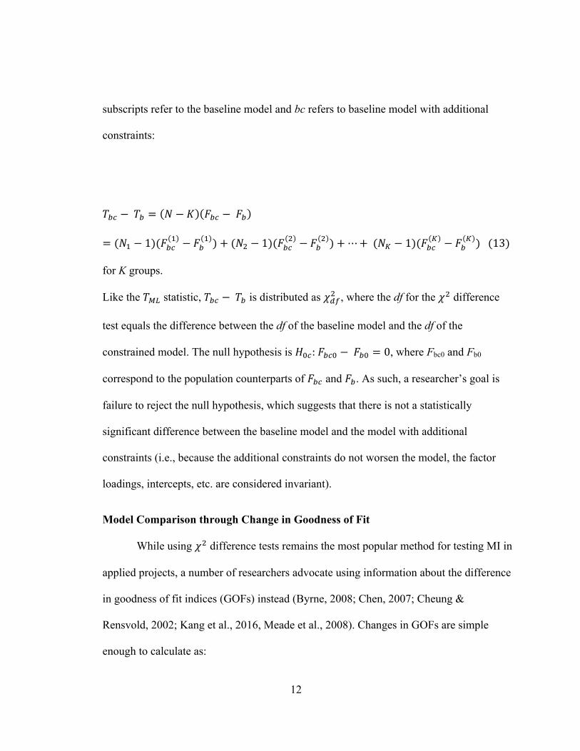
subscripts refer to the baseline model and bc refers to baseline model with additional
constraints:
𝑇!" − 𝑇! = 𝑁 − 𝐾 𝐹!" − 𝐹!
= (𝑁! − 1)(𝐹!"! − 𝐹!
! )+ (𝑁! − 1)(𝐹!"! − 𝐹!
! )+⋯+ (𝑁! − 1)(𝐹!"! − 𝐹!
! ) (13)
for K groups.
Like the 𝑇!" statistic, 𝑇!" − 𝑇! is distributed as 𝜒!"! , where the df for the 𝜒! difference
test equals the difference between the df of the baseline model and the df of the
constrained model. The null hypothesis is 𝐻!!: 𝐹!"! − 𝐹!! = 0, where Fbc0 and Fb0
correspond to the population counterparts of 𝐹!" and 𝐹!. As such, a researcher’s goal is
failure to reject the null hypothesis, which suggests that there is not a statistically
significant difference between the baseline model and the model with additional
constraints (i.e., because the additional constraints do not worsen the model, the factor
loadings, intercepts, etc. are considered invariant).
Model Comparison through Change in Goodness of Fit
While using 𝜒! difference tests remains the most popular method for testing MI in
applied projects, a number of researchers advocate using information about the difference
in goodness of fit indices (GOFs) instead (Byrne, 2008; Chen, 2007; Cheung &
Rensvold, 2002; Kang et al., 2016, Meade et al., 2008). Changes in GOFs are simple
enough to calculate as:
13
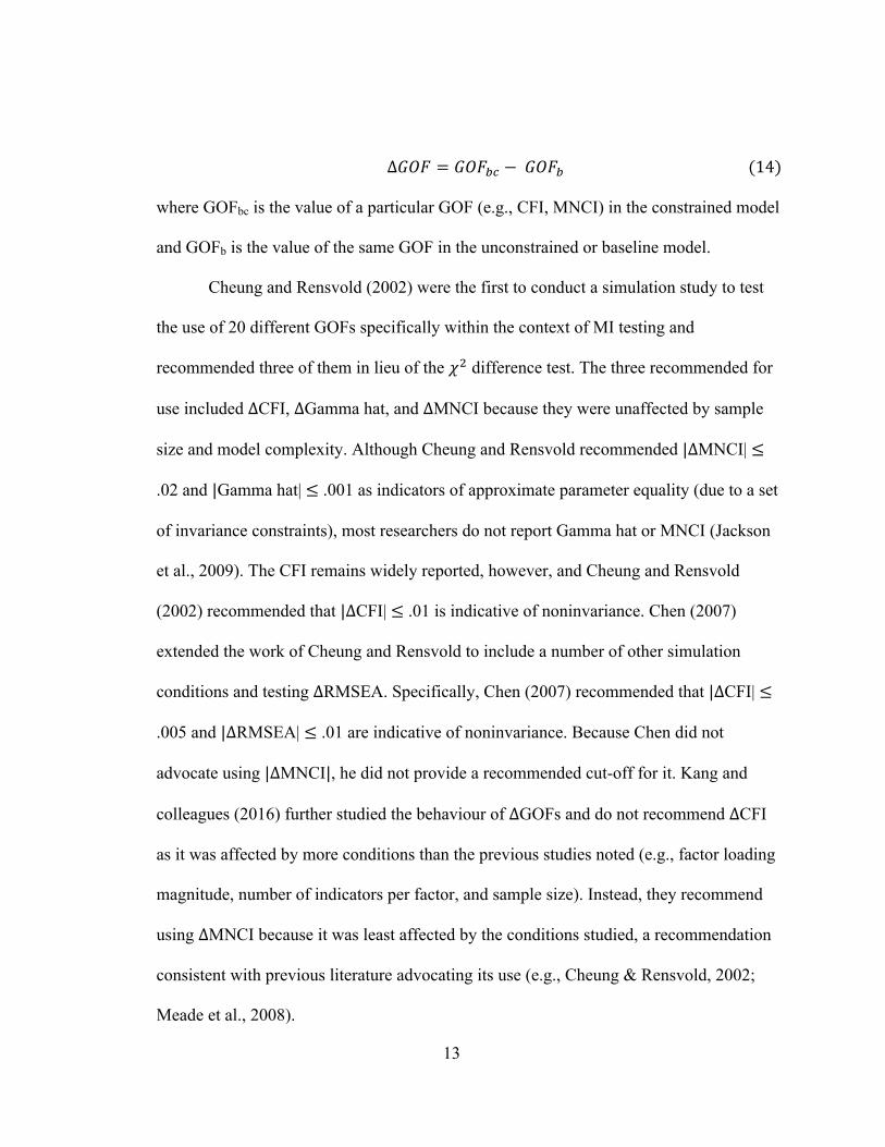
∆𝐺𝑂𝐹 = 𝐺𝑂𝐹!" − 𝐺𝑂𝐹! (14)
where GOFbc is the value of a particular GOF (e.g., CFI, MNCI) in the constrained model
and GOFb is the value of the same GOF in the unconstrained or baseline model.
Cheung and Rensvold (2002) were the first to conduct a simulation study to test
the use of 20 different GOFs specifically within the context of MI testing and
recommended three of them in lieu of the 𝜒! difference test. The three recommended for
use included ∆CFI, ∆Gamma hat, and ∆MNCI because they were unaffected by sample
size and model complexity. Although Cheung and Rensvold recommended |∆MNCI| ≤
.02 and |Gamma hat| ≤ .001 as indicators of approximate parameter equality (due to a set
of invariance constraints), most researchers do not report Gamma hat or MNCI (Jackson
et al., 2009). The CFI remains widely reported, however, and Cheung and Rensvold
(2002) recommended that |∆CFI| ≤ .01 is indicative of noninvariance. Chen (2007)
extended the work of Cheung and Rensvold to include a number of other simulation
conditions and testing ∆RMSEA. Specifically, Chen (2007) recommended that |∆CFI| ≤
.005 and |∆RMSEA| ≤ .01 are indicative of noninvariance. Because Chen did not
advocate using |∆MNCI|, he did not provide a recommended cut-off for it. Kang and
colleagues (2016) further studied the behaviour of ∆GOFs and do not recommend ∆CFI
as it was affected by more conditions than the previous studies noted (e.g., factor loading
magnitude, number of indicators per factor, and sample size). Instead, they recommend
using ∆MNCI because it was least affected by the conditions studied, a recommendation
consistent with previous literature advocating its use (e.g., Cheung & Rensvold, 2002;
Meade et al., 2008).

14
The two methods for nested model comparison described above, namely using
non-significant results from a 𝜒! difference test and using ∆GOF cut-offs, both have
important limitations. With the 𝜒! difference test, the researcher’s goal is aligned with
the null hypothesis, and failing to reject the null hypothesis does not provide support for
the researcher’s proposed goal of establishing MI. In other words, failing to reject 𝐻!!
does not imply that the models are equivalent across the groups, only that there is not
enough information to warrant rejecting 𝐻!!. This situation is particularly problematic
because the 𝜒! statistic almost always has high power to detect differences between the
models with the larger sample sizes typically seen in CFA or SEM models (Byrne, 2008;
MacCallum et al., 1996; Saris, Satorra, & van der Veld, 2009). One criticism of using
∆GOFs like CFI or RMSEA is the lack of consistent cut-offs values from simulation
research. This limitation is unsurprising though, when one considers that GOFs are
simply descriptive in nature with no known sampling distributions. This fact led Yuan,
Chan, Marcoulides, and Bentler (2016) to argue that researchers cannot use them to
advance the inferential value of a model. This criticism led Yuan and colleagues (2016)
to recommend calculating an appropriate test statistic that allows for a small degree of
model misspecification in SEM or CFA models. The difference is that they advocate
replacing these traditional MI approaches with equivalence testing, an area of research
that focuses on valid and logical statistics when a researcher’s goal is aligned with the
traditional null hypothesis. Equivalence testing is the topic of the next chapter.
15
CHAPTER TWO
APPLYING EQUIVALENCE TESTING TO MEASUREMENT INVARIANCE
Before detailing the available equivalence testing methods for MI, I provide
background information for the field of equivalence testing as well as a rationale for why
its application to MI is pertinent.
Equivalence Testing
Equivalence testing is a field of statistics used when the researcher’s hypothesis of
interest is the opposite of the traditional hypothesis testing (e.g., no mean difference).
Specifically, equivalence tests are used when the goal is to demonstrate a lack of
association among variables, which could mean that population means are equivalent
(e.g., Anderson & Hauck, 1983; Koh & Cribbie, 2013; Mara & Cribbie, 2012; Nasiakos,
Cribbie, & Arpin-Cribbie, 2010; Schuirmann, 1987; Wellek, 2010; Westlake, 1972), a
population correlation is minimal (e.g., Goertzen & Cribbie, 2010), population
correlations or regression coefficients do not differ across groups (e.g., Counsell &
Cribbie, 2015), categorical variables do not interact in the population (Cribbie,
Ragoonanan, & Counsell, 2016), and so on.
Equivalence tests have not been particularly popular in psychology despite their
numerous applications in a wide variety of substantive areas (Cribbie & Arpin-Cribbie,
2009; Cribbie, Gruman, & Arpin-Cribbie, 2004; Kendall, Marrs-Garcia, Nath, &
Sheldrick, 1999; Quertemont, 2011; Rogers, Howard, & Vessey, 1993; Seaman & Serlin,
1998). The benefit of equivalence testing is that it provides a statistically and

16
theoretically valid approach when a researcher’s goal is more closely aligned with
supporting the traditional null hypothesis instead of the alternative hypothesis. Accepting
the null hypothesis is inappropriate for establishing equivalence because researchers can
never statistically determine that the null hypothesis is true. In the words of Altman and
Bland (1995), absence of evidence is not evidence of absence. One of the biggest
strengths of equivalence testing is its ability to incorporate an interval that represents the
smallest meaningful difference into the null hypothesis instead of being forced to use a
null hypothesis with an effect exactly equal to zero. This benefit is an important one,
because with sampling error, even if the effect of interest were zero in the population, it is
unlikely that it will realize in a sample. This interval is called an equivalence interval, and
is described below.
Equivalence Intervals
In order to conduct an equivalence test, however, one must specify an a priori
equivalence interval (EI) such that any effect contained within the interval is considered
negligible or inconsequential, and thus, equivalence can be concluded. This EI depends
on a number of factors such as the nature of the research, which statistical test is used,
and so on. As an example, if a researcher sought to demonstrate that males and females
have equivalent IQs, she might choose an equivalence interval of +/- 1 SD. Since we
know that the average IQ is 100 with a standard deviation of 15, absolute mean
differences of less than 15 would be considered equivalent in this framework. Details of
how to apply an EI within the context of MI are provided in a subsequent section below.

17
Equivalence Testing Methods for Measurement Invariance
In traditional approaches to MI, the statistical goal is to retain the null hypothesis
that multiple groups’ factor structures and parameters (e.g., loadings, intercepts) are the
same. As a first step, researchers often seek a nonsignificant 𝑇!" in each group to
conclude good model fit and evidence of configural invariance. In later stages when using
𝜒! difference tests, the goal is to find a statistically non-significant result because one
does not want to find discrepancies between the parameters of different groups. As
detailed in both Yuan and Chan (2016) and Yuan and Bentler (2004), this strategy does
not control Type I or Type II errors when there is any amount of model misspecification,
that is, the estimated model is not perfectly equivalent to the population model or the
group parameters are not identical. This issue arises because with any amount of model
misspecification, the TML statistic is no longer distributed as 𝜒!, instead it follows a
noncentral 𝜒!distribution.
Given the statistical issues with accepting the null hypothesis in CFA models,
Yuan and Chan (2016) have proposed using equivalence testing methods to investigate
MI. They outline two equivalence testing approaches that allow for a small amount of
model misspecification by incorporating a noncentrality parameter into the null
hypothesis. The first test is used in lieu of the regular 𝑇!" to assess model fit and the
second test is the equivalence-based version of the 𝜒! difference test.
TML equivalence test
The first equivalence test proposed by Yuan and Chan (2016) evaluates model fit
by allowing for a small degree of model misspecification. While this test can be used in

18
single-group CFA or SEM models generally, it is relevant to MI because it is used at the
configural stage to ensure that the same factor structure fits well in each group separately.
This procedure uses the same 𝑇!" statistic in Equation 4, but the equivalence test version
has a different null hypothesis. More specifically, its null hypothesis is 𝐻!: 𝐹!"! > 𝜀!,
where 𝐹!"! is the population counterpart of 𝐹!" and 𝜀! is a positive number that the
researcher can tolerate for the size of misspecification, that is, the value for the EI. The
value of 𝜀! is used to calculate the corresponding noncentrality parameter (𝛿) where:
𝛿 = (𝑁 − 𝐾) 𝜀! (15)
With 𝑐!(𝜀!) as the left-tail critical value of the noncentral 𝜒!"! (𝛿) at cumulative
probability 𝛼, one rejects 𝐻!when 𝑇!" ≤ 𝑐!(𝜀!). Rejection of the null hypothesis implies
that the model misspecification is smaller than the pre-specified equivalence bound, 𝜀!
(Yuan & Chan, 2016) and one concludes that any differences between the sample
covariance matrix and model implied covariance matrix is trivial or inconsequential.
Using this method within the context of MI would require rejection of H0: 𝐹!"! > 𝜀! in
both groups to conclude that configural invariance is satisfied.
Equivalence testing alternative to the 𝝌𝟐 difference test
In testing the stages of MI, it is common to use 𝜒! difference tests to compare the
nested models. Using the modified 𝑇!" statistic outlined in Equation 13 and following the
same logic as their equivalence test for single group CFA models, Yuan and Chan (2016)
outline an equivalence test for 𝑇!" − 𝑇!. Its null hypothesis is 𝐻!: 𝐹!"! − 𝐹!! > 𝜀!.
One rejects the null hypothesis when 𝑇!" − 𝑇! ≤ 𝑐!(𝜀!), where 𝑐!(𝜀!) is defined above.

19
If a statistically significant result is obtained, the researcher can conclude that the added
equality constraints do not significantly worsen the model fit compared to the less
constrained model. Consequently, the researcher would conclude that metric, scalar, or
strict invariance is met depending on which stage is currently being tested.
What is an appropriate equivalence interval?
Since the value of 𝜀! is crucial to conducting Yuan and Chan’s (2016)
equivalence tests for MI, it is important to discuss how one chooses its value. In their
paper, 𝜀! represents the largest amount of model misspecification a researcher is willing
to accept. Choosing reasonable values for 𝜀!, however, is not immediately evident. Thus,
Yuan and Chan (2016) and Yuan et al. (2016) relate 𝜀! to the RMSEA based on the work
of Steiger (1998):
𝜀! = 𝑑𝑓 𝑅𝑀𝑆𝐸𝐴! !/𝐾 (16)
where 𝑅𝑀𝑆𝐸𝐴! is the a priori value of RMSEA that a researcher is willing to accept as a
reasonable amount of misspecification (e.g., .05, .08) and df is the model degrees of
freedom in a single group case or difference in df when comparing nested models. An
important consideration worth highlighting is that for a given value of 𝑅𝑀𝑆𝐸𝐴!, 𝜀!
changes depending on the model df. The implication is that a researcher cannot
effectively choose a single value for 𝜀! to be applied to multiple models like is typically
done with a simple adoption of Hu and Bentler’s (1999) fit index recommendations. As
an aside, common recommendations for GOFs (e.g., Hu & Bentler, 1999) were not meant
for use as strict cut-off values either, but applied researchers typically use them as such.

20
Yuan and colleagues (2016) argued in favour of a standard for choosing the value
of 𝜀! and proposed using MacCallum et al.’s (1996) RMSEA guidelines of .01, .05, .08,
and .10 for excellent, close, fair, mediocre, and poor fitting models. They later noted,
however, that using these guidelines to calculate values of 𝜀! in the equivalence test
results in too stringent an amount of model misspecification compared to using them with
the traditional point estimate null hypothesis. To remedy this issue, they created adjusted
RMSEA values for use in calculating 𝜀! and propose that these should be the new norm
for cut-offs in the equivalence test (Yuan et al., 2016; Yuan & Chan, 2016). Their
adjusted RMSEA values are calculated as follows:
Step 1: Calculate a 𝑇!" statistic based on the following formula:
𝑇!" = 𝑑𝑓 𝑁 − 𝐾𝑅𝑀𝑆𝐸𝐴!!
𝐾 + 𝑑𝑓 (17)
where RMSEAc denotes a conventional RMSEA value (e.g., .01 or .05).
Step 2: Using the 𝑇!" calculated in Step 1, find the value of 𝜀! such that 𝑇!" = 𝑐!(𝜀!)
based on a noncentral 𝜒!"! (𝛿), where 𝛿 is defined above in Equation 15.
Step 3: Using Equation 15, calculate the value of the RMSEA0 based on the value of 𝜀!
obtained from Step 2.
Step 4: In a linear regression model, use N, K, df, and RMSEAc to predict ln(RMSEA0).
Once the predicted value ya is obtained, calculate exp(ya) and use this value as the
adjusted RMSEA.

21
The exact details of the regression analysis can be seen in Table 12 in Yuan and Chan
(2016). They also provide a function to calculate the adjusted RMSEA at conventional
values of .01, .05, .08, and .10.
One issue with Yuan and Chan’s (2016) adjusted RMSEA is the lack of numerical
evaluation into why a researcher should use this value for 𝜀! instead. Their theoretical
justification is that the probability of rejecting the null hypothesis decreases as one
proceeds to testing later stages of MI due to the sequential nature of the nested model
comparisons. In fact, with just two groups, the probability is raised to the 5th power to
reach the end of the sequence (𝐻!! ,𝐻!! → 𝐻! → 𝐻! → 𝐻!). While this sequence
certainly results in decreased power and evidence that traditional RMSEA values may be
too stringent, it is unclear exactly how their proposed adjusted RMSEA remedies this
problem.
The Test of Close Fit
Yuan and Chan’s (2016) proposed equivalence tests are incredibly similar to the
test of close fit approach discussed in previous research (Browne & Cudeck, 1992;
MacCallum et al., 1996; MacCallum, Browne, & Cai, 2006; Preacher, Cai, &
MacCallum, 2007). Browne and Cudeck’s test of small difference is: 𝐻!: 𝜀 ≤ .05, where
.05 is in RMSEA units. The implication is that in order to conclude a good fitting model,
the researcher is still trying to ‘accept’ rather than reject a null hypothesis. MacCallum
and colleagues extended the work to a ‘Good-Enough Principle’, which allows for other
values of 𝜀 derived from the noncentrality parameter, similar to Yuan and Chan’s work.
The main difference between these tests surrounds the calculation of the noncentrality

22
parameter. Yuan and Chan’s (2016) method uses one RMSEA value to calculate 𝜀 and 𝛿
(see Equations 15 and 16), whereas MacCallum et al.’s work uses two RMSEA values
(each labeled 𝜀), one specified for each of the two nested models. Their calculation of 𝛿
is:
𝛿 = 𝑁(𝑑𝑓!"𝜀!"!! − 𝑑𝑓!𝜀!!! ) (18)
where 𝜀 is a raw RMSEA value. MacCallum and colleagues did not discuss the method
within the larger equivalence testing framework, but the logic and execution of the tests
are the same.

23
CHAPTER THREE
METHOD AND RESULTS
Method
A simulation study was used to evaluate the performance of Yuan and Chan’s
(2016) equivalence tests. Specifically, rates of rejection under Type I error and power
conditions were recorded and compared for the original equivalence test (EQ) and EQ
using the adjusted values of 𝜀! (EQ-A). These results were compared to those obtained
using a traditional 𝜒! difference test (TCS) with a statistically non-significant result (i.e.,
p > α) and using recommended ∆GOFs for CFI, RMSEA, and MNCI. At the configural
stage, the GOF cut-offs were .95 for CFI, .95 for MNCI and values of the RMSEA that
corresponded to what was used to calculate 𝜀! (i.e., .05, .08, and .10). Cut-offs used for
the ∆GOFs at the metric, scalar, and strict invariance stages were taken from Chen
(2007). Invariance was concluded if the CFI of the more constrained model did not
decrease by more than .005, the RMSEA did not increase by more than .01, and the
MNCI did not decrease by more than .01. The simulation was run with R (R Core Team,
2016), and data generation and analysis both were done using the lavaan package
(Rosseel, 2012). Data were generated by specifying a population CFA model separately
for each of the two groups and then randomly sampling data that matched each group’s
model-implied covariance matrix.
A number of conditions were manipulated in the study. These manipulations
included the number of indicators in the measurement model (one with four indicators
per factor and one with eight indicators per factor), size of the factor loadings (.5, .7, or .9

24
with error variances corresponding to .75, .51, and .19 respectively), size of the
equivalence bounds (calculated from population RMSEA values of .05, .08, or .10,
referred to as EI05, EI08, EI10 respectively), sample size per group (100, 250, 500, 1000,
or 2000), and whether the population models are characterized by MI (which is a power
condition in the equivalence testing perspective) or not (Type I error condition for
equivalence testing). In all conditions, the population correlation between the latent
variables was .5, and there were no error covariances among the indicators (except in
specific Type I error conditions at the configural stage, see below). Figure 1 includes the
path diagrams for each of the measurement models. The configural invariance models
were estimated such that the latent variables in each group were standardized (for
identification) and all other parameters were freely estimated. The metric invariance
model allowed the variance of the latent variables to be freely estimated and the model
was identified by setting the scales of the latent variables using the first indicator’s
loading on each latent variable with across-group equality constraints on the rest of the
indicators’ loadings. The scalar invariance model freed the means of the latent variables
in addition to their variances and included across-group equality constraints on all of the
indicator’s intercepts. Finally, the strict invariance model added group equality
constraints on the error variances.
The simulation conditions were chosen to reflect situations that occur in
psychological research. The sample sizes chosen represent a reasonable range of potential
sample sizes that are typically seen with SEM models in psychology. Jackson and
colleagues (2009) found a median sample size of 389 in the surveyed SEM/CFA studies
25
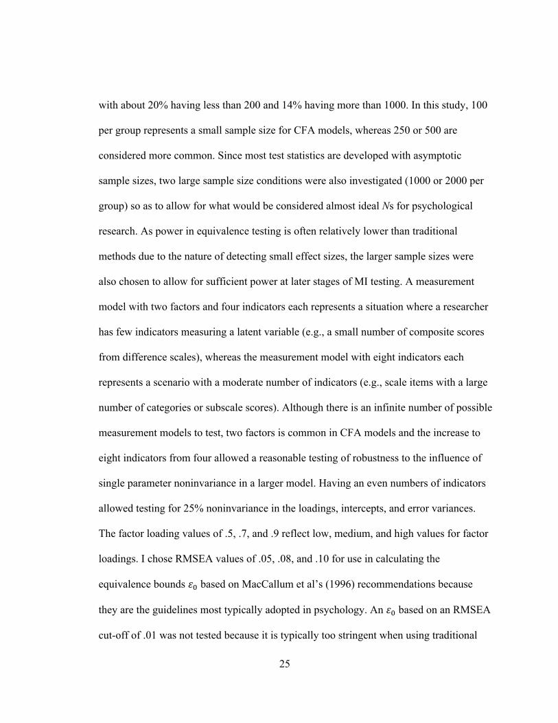
with about 20% having less than 200 and 14% having more than 1000. In this study, 100
per group represents a small sample size for CFA models, whereas 250 or 500 are
considered more common. Since most test statistics are developed with asymptotic
sample sizes, two large sample size conditions were also investigated (1000 or 2000 per
group) so as to allow for what would be considered almost ideal Ns for psychological
research. As power in equivalence testing is often relatively lower than traditional
methods due to the nature of detecting small effect sizes, the larger sample sizes were
also chosen to allow for sufficient power at later stages of MI testing. A measurement
model with two factors and four indicators each represents a situation where a researcher
has few indicators measuring a latent variable (e.g., a small number of composite scores
from difference scales), whereas the measurement model with eight indicators each
represents a scenario with a moderate number of indicators (e.g., scale items with a large
number of categories or subscale scores). Although there is an infinite number of possible
measurement models to test, two factors is common in CFA models and the increase to
eight indicators from four allowed a reasonable testing of robustness to the influence of
single parameter noninvariance in a larger model. Having an even numbers of indicators
allowed testing for 25% noninvariance in the loadings, intercepts, and error variances.
The factor loading values of .5, .7, and .9 reflect low, medium, and high values for factor
loadings. I chose RMSEA values of .05, .08, and .10 for use in calculating the
equivalence bounds 𝜀! based on MacCallum et al’s (1996) recommendations because
they are the guidelines most typically adopted in psychology. An 𝜀! based on an RMSEA
cut-off of .01 was not tested because it is typically too stringent when using traditional

26
methods and overly restrictive in equivalence testing as outlined in both Yuan et al.
(2016) and Yuan and Chan (2016).
Power Conditions
Two different power conditions were investigated in the simulation. In the first
condition, the population CFA models were exactly equivalent between each of the
groups. In the second power condition, the population models were not identical, but the
differences between them were minute, such that the amount of model misspecification
was considered small enough to conclude invariance. Specifically, it was set at 10% of
𝜀! using a population RMSEA of .10, which was always smaller than each of the EIs
(based on RMSEA0 = .05, .08, or .10). See Table 1 for the exact differences in model
misfit for the second power condition.
Because power rates for later stages are calculated only when the previous MI
stages have been met, the discrepancy between population models as one moves through
the stages is not additive for the conditions with a small degree of misspecification or
group differences. Using metric invariance as an example, power rates at this stage are
calculated with a small degree of model misspecification in a loading, but the small
degree of misspecification that was previously in the configural invariance stage would
no longer be present. Regardless of whether the groups’ population models were identical
or had small differences, power rates for the metric, scalar, and strict invariance stages all
take into consideration whether the previous stages have been met or not. For example, if
testing metric invariance in a given replication, a missing value would be recorded in lieu
of a p value if configural invariance had not been met in the same replication. The
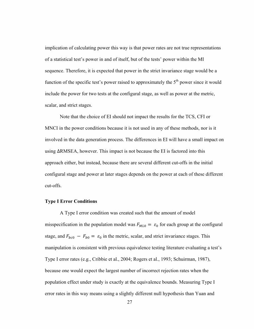
27
implication of calculating power this way is that power rates are not true representations
of a statistical test’s power in and of itself, but of the tests’ power within the MI
sequence. Therefore, it is expected that power in the strict invariance stage would be a
function of the specific test’s power raised to approximately the 5th power since it would
include the power for two tests at the configural stage, as well as power at the metric,
scalar, and strict stages.
Note that the choice of EI should not impact the results for the TCS, CFI or
MNCI in the power conditions because it is not used in any of these methods, nor is it
involved in the data generation process. The differences in EI will have a small impact on
using ∆RMSEA, however. This impact is not because the EI is factored into this
approach either, but instead, because there are several different cut-offs in the initial
configural stage and power at later stages depends on the power at each of these different
cut-offs.
Type I Error Conditions
A Type I error condition was created such that the amount of model
misspecification in the population model was 𝐹!"! = 𝜀! for each group at the configural
stage, and 𝐹!"! − 𝐹!! = 𝜀! in the metric, scalar, and strict invariance stages. This
manipulation is consistent with previous equivalence testing literature evaluating a test’s
Type I error rates (e.g., Cribbie et al., 2004; Rogers et al., 1993; Schuirman, 1987),
because one would expect the largest number of incorrect rejection rates when the
population effect under study is exactly at the equivalence bounds. Measuring Type I
error rates in this way means using a slightly different null hypothesis than Yuan and

28
Chan (2016). Their tests’ null hypotheses were 𝐹!"! > 𝜀! and 𝐹!"! − 𝐹!! > 𝜀!,
whereas the null hypotheses I use (which are more consistent with the equivalence testing
literature) are 𝐹!"! ≥ 𝜀! and 𝐹!"! − 𝐹!! ≥ 𝜀!. Although the difference is subtle, the
implication is that Yuan and Chan consider 𝜀! to be the largest amount of model
misspecification one is willing to tolerate for concluding invariance, whereas I consider
𝜀! to be the smallest amount of model misspecification that a researcher would deem a
meaningful difference and would, therefore, be considered noninvariance.
The amount of model misspecification when testing error rates at later stages
included only the misspecification at that level, such that invariance was met in the
previous stages. For example, when assessing the error rates for scalar invariance, the
amount of model misspecification, 𝐹!"! − 𝐹!! = 𝜀! occurred only in the intercepts and
not in any of the other model parameters implicated in configural or metric invariance.
To violate configural invariance, error covariances were added to different pairs
of indicators in each group. In group one, a covariance was added between the first
indicators on each factor and in group two, a covariance was added between the second
indicators on each factor. The magnitude of the covariances varied by population
measurement model, factor loading magnitude, and EI in each condition. To violate
metric, scalar, or strict invariance, I tested two separate Type I error conditions. In the
first, a single parameter (loading, intercept, or error variance) was noninvariant across the
two groups; in the second, 25% of the parameters were noninvariant across the two
groups. Refer to Table 2 for the exact differences in population models across the various
Type I error conditions.
29
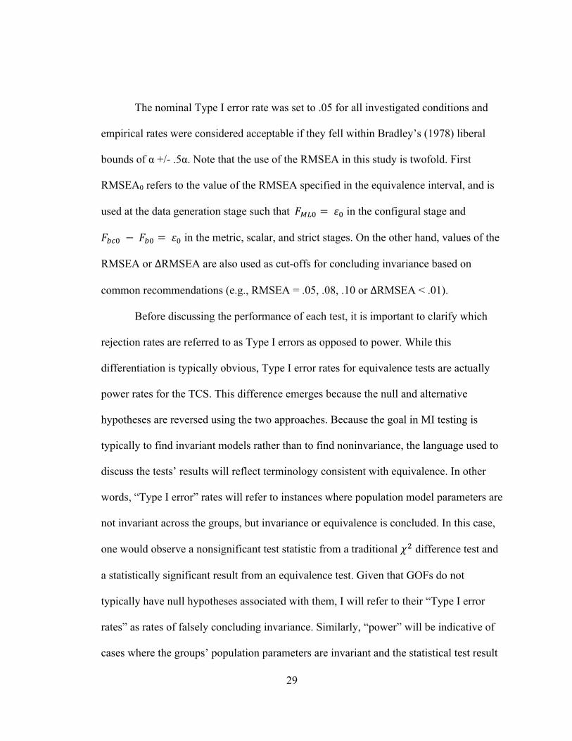
The nominal Type I error rate was set to .05 for all investigated conditions and
empirical rates were considered acceptable if they fell within Bradley’s (1978) liberal
bounds of α +/- .5α. Note that the use of the RMSEA in this study is twofold. First
RMSEA0 refers to the value of the RMSEA specified in the equivalence interval, and is
used at the data generation stage such that 𝐹!"! = 𝜀! in the configural stage and
𝐹!"! − 𝐹!! = 𝜀! in the metric, scalar, and strict stages. On the other hand, values of the
RMSEA or ∆RMSEA are also used as cut-offs for concluding invariance based on
common recommendations (e.g., RMSEA = .05, .08, .10 or ∆RMSEA < .01).
Before discussing the performance of each test, it is important to clarify which
rejection rates are referred to as Type I errors as opposed to power. While this
differentiation is typically obvious, Type I error rates for equivalence tests are actually
power rates for the TCS. This difference emerges because the null and alternative
hypotheses are reversed using the two approaches. Because the goal in MI testing is
typically to find invariant models rather than to find noninvariance, the language used to
discuss the tests’ results will reflect terminology consistent with equivalence. In other
words, “Type I error” rates will refer to instances where population model parameters are
not invariant across the groups, but invariance or equivalence is concluded. In this case,
one would observe a nonsignificant test statistic from a traditional 𝜒! difference test and
a statistically significant result from an equivalence test. Given that GOFs do not
typically have null hypotheses associated with them, I will refer to their “Type I error
rates” as rates of falsely concluding invariance. Similarly, “power” will be indicative of
cases where the groups’ population parameters are invariant and the statistical test result

30
concludes group invariance or equivalence (i.e., nonsignificant traditional 𝜒! result and
significant equivalence test 𝜒! result). I will refer to these rates for GOFs as rates of
concluding invariance.

31
Results
Nonconvergence
Nonconvergence was not an issue in any of the models tested. Specifically, the
highest rate of nonconvergence was only 1.68% in the metric Type I error condition with
the smallest sample size condition tested (i.e., 100 per group) and factor loadings of .5 in
the four-indicator model. Rates of nonconvergence for sample sizes of 250 per group
were negligible (e.g., between 0 and 0.2%). All of the conditions with the eight-indicator
model demonstrated perfect convergence rates. Perfect convergence also occurred across
all conditions with the four-indicator model and sample sizes of at least 500 per group.
The highest rate of nonconvergence in the power conditions was 0.36%. Small rates of
nonconvergence occurred only with the smallest size conditions and weak factor loadings
(i.e., .5) in the four-indicator model and were zero in the rest of the power conditions. In
an iteration where the model failed to converge, the statistics were not collected and Type
I error or power rates were calculated with an adjusted denominator removing these
problematic results.
Empirical Type I error rates
Configural Invariance. Type I error rates at the configural invariance stage are
presented in Tables 3 to 8. As adequate model fit must first be demonstrated in each
group, Tables 3 through 6 contain information on model fit in each group as opposed to
true configural invariance rates. Tables 7 and 8 contain the rates of falsely concluding
configural invariance, which would ideally equal 𝛼!, because the Type I error rates in
each of the groups would be expected at 𝛼. It is worth noting that information in the

32
configural invariance tables for the different fit indices include rates of concluding
invariance only when both groups individually met the cut-offs for good model fit. I
could have presented results from the fit indices in the multi-group CFA as they were
also collected, but it is possible that one group could demonstrate relatively poor model
fit and another excellent model fit and could result in good overall fit. As expected, these
rates indeed resulted in higher rates of concluding invariance in both conditions.
In the four-indicator model, accurate empirical error rates were observed in the
equivalence test (EQ) regardless of sample size, population RMSEA value used in the EI,
or indicator loading. For the eight-indicator model, however, accurate error rates were
observed in the EIs based on an RMSEA of.05, but were inconsistent for EIs based on
RMSEAs of .08 or .10. Here, error rates were too low, typically less than 𝛼/2. The only
difference between these two models is the df (19 per group vs. 103 per group), which is
implicated in the calculation of the EI such that the eight-indicator model would have a
larger EI and noncentrality parameter overall. Given this unexpected result, I tested a ten-
indicator model (df = 169 per group) to see whether rates were even more conservative
than the four- and eight-indicator models and this pattern of results was observed.
Implications of this finding will be discussed in the last chapter.
Using the TCS, one would falsely conclude configural invariance too often at
smaller sample sizes (e.g., 100 per group) and a smaller EI (based on RMSEA of .05).
For conditions with larger sample sizes (i.e., 250 per group or larger) and EIs based on
RMSEA values of .08 or .10, rates of falsely concluding invariance were virtually zero,
as the test achieved sufficient power to detect small differences between the model-

33
implied covariance matrix and covariance matrix from the data. The EQ-A also did not
demonstrate accurate empirical Type I error rates. In the four-indicator model, the error
rates for falsely concluding configural invariance hovered around .25. Stated differently,
the test incorrectly concluded good model fit in each group approximately 50% of the
time regardless of EI, N, or factor loading. Under the conditions tested, the adjustment
provided an overcorrection to combat reduced power at the expense of the test’s Type I
error rates.
If one were to rely exclusively on the fit indices, CFI, MNCI, and RMSEA, rates
of falsely concluding configural invariance would be too high. For the .95 CFI cut-off, a
number of conditions interacted to affect these rates. With factor loadings of .5 and
equivalence bounds based on RMSEA = .05, rates of falsely concluding invariance
decreased as N increased. However, they were still too high with sample sizes less than
1000 per group. When the factor loadings were .7, the opposite result was observed with
equivalence bounds calculated from RMSEA0 values of .05 or.08; that is, their rates
increased as N increased and were too low with an RMSEA0 of .10. Lastly, when the
loadings were .9, configural invariance was concluded in almost every replication
regardless of condition.
For the MNCI, when data were generated from an RMSEA0 = .05, the test
concluded configural invariance in almost all of the replications. Its rates of falsely
concluding invariance increased as N increased, such that in the lowest sample size,
invariance was concluded 55% of the time. Unlike the CFI, this pattern did not depend on
the magnitude of the factor loadings. At RMSEA0 = .08, rates were too high at smaller
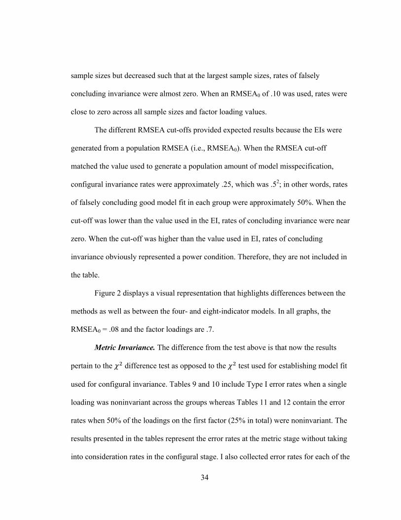
34
sample sizes but decreased such that at the largest sample sizes, rates of falsely
concluding invariance were almost zero. When an RMSEA0 of .10 was used, rates were
close to zero across all sample sizes and factor loading values.
The different RMSEA cut-offs provided expected results because the EIs were
generated from a population RMSEA (i.e., RMSEA0). When the RMSEA cut-off
matched the value used to generate a population amount of model misspecification,
configural invariance rates were approximately .25, which was .52; in other words, rates
of falsely concluding good model fit in each group were approximately 50%. When the
cut-off was lower than the value used in the EI, rates of concluding invariance were near
zero. When the cut-off was higher than the value used in EI, rates of concluding
invariance obviously represented a power condition. Therefore, they are not included in
the table.
Figure 2 displays a visual representation that highlights differences between the
methods as well as between the four- and eight-indicator models. In all graphs, the
RMSEA0 = .08 and the factor loadings are .7.
Metric Invariance. The difference from the test above is that now the results
pertain to the 𝜒! difference test as opposed to the 𝜒! test used for establishing model fit
used for configural invariance. Tables 9 and 10 include Type I error rates when a single
loading was noninvariant across the groups whereas Tables 11 and 12 contain the error
rates when 50% of the loadings on the first factor (25% in total) were noninvariant. The
results presented in the tables represent the error rates at the metric stage without taking
into consideration rates in the configural stage. I also collected error rates for each of the

35
tests only for the replications where configural invariance was met. These rates were
based on a smaller number of replications (configural power*5000), but the results were
almost identical to those presented in the tables.
The same pattern of findings for error rates observed at the configural invariance
stage was observed here. As expected, the EQ was the only method that consistently
demonstrated accurate Type I error rates. Its empirical error rates were not affected by
any of the conditions (i.e., measurement model, factor loading magnitude, single factor
noninvariance or multiple factor noninvariance, etc.). One difference is that error rates
were also accurate across the conditions in the eight-indicator model, whereas some
lower error rates were observed for these conditions in the configural stage. The EQ-A
had rates around .50 under all conditions except when the sample size was 2000 per
group whereby it decreased to rates close to .25.
Again, the TCS difference test had inaccurate rates of falsely concluding metric
invariance with rates as high as .81 at smaller sample sizes with EIs based on an RMSEA
of .05. As expected, these rates decreased as N increased, eventually reaching zero.
The rates of incorrectly concluding invariance using ∆GOF were also high in the
metric stage. Using ∆RMSEA demonstrated a similar pattern of results as the traditional
𝜒! difference test but the rates of falsely concluding invariance did not decrease as
rapidly using ∆RMSEA, particularly with model misspecification of RMSEA = .05 or
.08. Using the ∆CFI instead produced error rates that changed based on all of the
investigated conditions except for a single noninvariant loading condition compared with
the 25% noninvariance condition. Rates of falsely concluding metric invariance generally

36
increased as the factor loading values increased and were highest with an EI05. These
conditions also interacted, such that Type I error rates were lower as the EI increased and
typically too low with the EI08 and EI10 for medium to large sample sizes, but these
rates increase with increasing factor loadings as well. In the eight-indicator models,
regardless of EI, rates of falsely concluding invariance were close to 1 with factor
loadings of .9; however, these results only occurred with EI05 in the four-indicator
models with factor loadings of .9. Rates of falsely concluding metric invariance increased
with sample size with a model misspecification of RMSEA0 = .05, remained stable
between .5 and .6 with an RMSEA0 of .08, and decreased with sample size with an
RMSEA0 of .10 in the four-indicator model. The same pattern occurred with the eight-
indicator model except rates also decreased with N in the RMSEA0= .08 condition and
lower overall. These patterns did not differ according to whether there was a single
noninvariant loading or 25% noninvariant loadings.
Figure 3 displays a visual representation that highlights differences between the
methods as well as the CFI’s interaction with factor loading magnitude. In all graphs,
results are from the four-indicator model with a single loading being noninvariant based
on a population misspecification of RMSEA0 = .08.
Scalar Invariance. Type I error rates at the scalar stage were similar to those
observed in metric invariance stage. This finding is unsurprising since metric, scalar, and
strict invariance are all tested with the same method, that is, a 𝜒! difference test and its
EQ analogue or a ∆GOF based on the same cut-off criteria. Tables 13 and 14 include

37
error rates when a single intercept was noninvariant across the groups whereas Tables 15
and 16 contain the error rates when 25% of the intercepts were noninvariant.
Strict Invariance. Tables 17 and 18 include Type I error rates when a single error
variance was noninvariant across the groups and Tables 19 and 20 contain the error rates
when 25% of the error variances were noninvariant. Error rates at the scalar stage were
similar to those observed in previous stages as was highlighted in the section for scalar
invariance. For the EQ, error rates appear too conservative in the n = 100 per group
conditions, but this result occurred simply because the test does not have sufficient power
to detect differences in the strict invariance stage. Power results will be displayed in the
next section.
It was anticipated that the results for the EQ at the metric, scalar, and strict
invariance phases would be highly similar because they use the same statistical method,
that is, the EQ version of the 𝜒! difference test. While differences in error rates are likely
to emerge under assumption violation (e.g., non-normality, non-linearity, etc.), a
desirable property is that a test’s error rates are unaffected by data based on differences
such as number of indicators or factors, parameter estimates, or choice of EI. This pattern
was, indeed, demonstrated in the results for the EQ 𝜒! difference test, but the error
results differed depending on the size of the measurement model when attempting to
establish adequate model fit. The EQ-A test recommended by Yuan and Chan (2016) did
not have accurate error rates in any of the simulation conditions tested.

38
Empirical Power Rates
Before discussing the power results below, it is important to note that different
tests’ power rates cannot be compared fairly unless accurate Type I error rates are
observed in the same condition. For easy comparison, power rates in bold represent
conditions with accurate Type I error rates. Note also that while this language does not
validly apply to using GOFs, the same procedure is applied such “power” rates (i.e., rates
of correctly concluding invariance) as in bold in conditions where their rates of falsely
concluding invariance were close to 𝛼.
Configural Invariance. Power rates for configural invariance when each group
had an identical population model are presented in Tables 21 to 26. Power rates when
there was a small amount of model misspecification in the population models, but the
amount is contained within 𝜀!, are presented in Tables 27 to 32. Once again, rates for
concluding configural invariance were calculated from the power for the individual
groups meeting the cut-offs as opposed to examining the fit indices from the multi-group
CFA.
With zero model misspecification, rates for concluding invariance using the TCS
do not change as a function of sample size. This result is expected, as this is actually a
Type I error condition for the TCS in traditional difference-based testing, and therefore
rates of concluding invariance would be expected to be approximately 1-𝛼 (.95). Rates of
.95 were indeed observed in the single group models, which can be seen in Tables 21 to
24. Because overall rates of configural invariance depend on the rates concluding good

39
model fit in each group, one would expect to conclude configural invariance in 100(1-
𝛼)2% of replications, as seen in Tables 25 and 26. However, with a small level of model
misspecification, rates of correctly concluding good model fit and configural invariance
using the TCS method decrease as the sample size increases. In the larger sample size
conditions, configural invariance is almost never concluded because the TCS has reached
almost 100% power to detect small amounts of model misspecification.
The EQ and EQ-A both demonstrate valid statistical relationships between sample
size and power regardless of condition. In other words, as N increases, so does the tests’
power. A ceiling effect is observed in the EQ-A test though, where it has almost 100%
power even at low sample sizes. This result is a function of its Type I error rate, however,
because it was falsely concluding good model fit in each group almost 50% of the time
across the same conditions. Power rates for the EQ’s ability to demonstrate good model
fit are low at small sample sizes (100 or 250 per group) when the EI is based on an
RMSEA of .05, but they increase rapidly as one increases the EI (through higher RMSEA
values or a larger df model) and as N increases.
Rates of concluding invariance using the CFI cut-off resulted in a similar pattern
of results as was seen in the Type I error conditions whereby higher loadings resulted in
increased rates of concluding invariance. This pattern was not observed in the MNCI. Its
rates of concluding invariance increased only as a function of sample size. The same
pattern was observed for the various RMSEA cut-offs and, unsurprisingly, power
increased as the RMSEA cut-off increased. Rates of concluding invariance using the
40
GOF indices were very high even at small sample sizes, due in part to the fact that they
had high rates of concluding invariance when the population model was misspecified.
Using the EQ, EQ-A, or GOF indices, the same pattern of results holds when
there is a small degree of model misspecification, but the rates for concluding good
model fit and configural invariance are simply lower. Note the difficulty in properly
comparing the magnitude of these rates for the EQ and other methods because the rates of
incorrectly concluding invariance (e.g., Type I error in EQ and EQ-A) are quite different.
Metric Invariance. Power rates for metric invariance when each group has an
identical population model are presented in Tables 33 and 34. Power rates for metric
invariance with small population differences in a loading between the groups are
presented in Tables 35 and 36. The pattern of results for the TCS, EQ, and EQ-A all
remained the same as what was observed among the configural invariance power rates.
Specifically, the TCS demonstrated an inappropriate relationship between rates of
concluding invariance and sample size, whereas the EQ and EQ-A had power rates that
increased appropriately as sample size increased. One difference, however, is that now
rates of concluding invariance are lower because these rates at the configural stage gets
factored into the rates of concluding metric invariance.
Slight differences in ∆GOF are observed due to differences in cut-offs from
moving to a 𝜒! difference test from single-group 𝜒! tests of model fit. While the power
rates using a ∆RMSEA appear to be affected by the value of the EI, the differences
between the conditions instead emerge due to different cut-offs in the configural stage. If
one were to ignore the power rates in the configural stage, they would be equivalent
41
across the different EI values in the metric stage like what is seen when using the MNCI
or CFI. When the groups’ population models were identical, the rates of concluding
invariance using a ∆MNCI or ∆CFI were lower in the eight-indicator model compared to
the four-indicator model, whereas they were higher using ∆RMSEA.
Scalar Invariance. Power rates for scalar invariance when each group has an
identical population model are presented in Tables 37 and 38. Tables 39 and 40 include
rates when a single intercept is slightly different between the groups’ population models.
Unsurprisingly, the same pattern of results held as was observed at the metric invariance
level although rates of concluding invariance are further impacted by rates by each of the
previous stages due to the sequential testing of MI. With sample sizes of 100 per group,
the EQ had power rates of virtually zero regardless of EI. Using the EI08 or EI10, a
researcher would still probably need around 500 people per group to have sufficient
power to test scalar invariance in a smaller model (e.g., a four-indicator model). Having a
larger df model (e.g., an eight-indicator) results in an increase in power, whereby the test
has reasonable power with 250 per group if using EI08 or EI10. Using the EI05, even
with a sample size of 500 per group, only about 50% power is observed.
Strict Invariance. Power rates for strict invariance are presented in Tables 41 to
44. The first two tables include rates for identical group population models and the
following tables include rates when a single error variance differs to a small degree
between the population models. Power results in the strict invariance level are similar to
those discussed in the previous stages, but are substantially lower due to the sequential

42
testing (i.e., power5). Rates for the EQ are quite low, particularly when the population
models are not identical, with EI05s, and when the model has a lower df.
Figure 4 includes a visual representation of the rates of correctly concluding
invariance at both the configural invariance and metric invariance stages. The results for
configural invariance represent the model fit in a single group to highlight the power of
the EQ without the sequential impact of MI. The metric invariance rates show power
results where rates of concluding invariance at previous stages in the sequence are taken
into consideration. Figure 4 does not present rates of concluding invariance for the EQ-A
or fit indices due to ceiling effects.

43
CHAPTER FOUR
EMPIRICAL EXAMPLE
To demonstrate differences between traditional methods for MI and the
equivalence testing methods proposed by Yuan and Chan (2016), I obtained data from a
large scale personality testing website (http://personality-testing.info/) and compared the
equivalence test (EQ) to the other traditional methods. Note that I demonstrate the EQ
method and not the EQ-A due to its poor performance in the simulation study.
The obtained data came from the Generic Conspiracist Beliefs Scale (GCB;
Brotherton, French, & Pickering, 2013), which included item-level information on the
scale as well as demographic variables. The scale includes 15 items measuring the degree
to which individuals endorse the item. The response to each item is given on a 5-point
Likert-type scale ranging from 1 = definitely not true to 5 = definitely true. The 15 items
comprise five subscales measuring belief in different types of conspiracies. Each subscale
has three items that load solely on that subscale (i.e., no cross loadings). The subscales
are government malfeasance, extra-terrestrial cover-up, malevolent global conspiracies,
personal wellbeing, and information control. The subscales are hypothesized to correlate
with one another. See Figure 5 for a path diagram of the GCB’s measurement model.
I decided to test MI on the scale using gender (male vs. female) as the grouping
variable to determine whether the scale functions equivalently across the two genders.
Previous research by Darwin, Neave, and Holmes (2011) and Bruder et al. (2013) did not
find meaningful differences between males and females on belief in conspiracies based
on mean testing procedures. Their conclusions were drawn from nonsignificant t-tests of
44
observed subscale scores though; they did not investigate MI. The dataset I used included
2359 participants, 1222 males and 1137 females. There were no missing data on any of
the items on the GCB scale for either group.
For each of the MI steps, I estimated multi-group CFA models using the lavaan
package (Rosseel, 2012) in R/RStudio (R Core Team, 2016; RStudio Team, 2016).
Although the indicators are categorical, I used maximum likelihood (ML) estimation for
the models. Previous research suggests that with at least five categories, approximately
normal response distributions and large sample sizes, ML estimation appropriate
(Rhemtulla, Brosseau-Liard, & Savalei, 2012). The parameter estimates for the male only
model can be seen in Table 44 and the parameter estimates for the female only model are
included in Table 45.
Results Using the Traditional Methods for MI The initial step involved establishing configural invariance, or demonstrating that
each group’s data follow the same hypothesized factor structure. Estimating the
hypothesized model for the males resulted in a statistically significant 𝑇!" statistic,
𝜒!(80) = 408.79, p < .001. The same result was observed for the female group, 𝜒!(80) =
364.92, p < .001. If a researcher relied on the 𝑇!" test alone, configural invariance cannot
be concluded and therefore, one could not proceed to test the invariance of loadings,
intercepts or error variances. In practice, however, it is rare that a researcher would rely
exclusively on the 𝑇!" statistic to assess model fit. Because each group demonstrated
good model fit based on the CFI (male = .973, female = .971) and RMSEA (male = .056
and female = .058), I will test metric invariance using the 𝜒! difference approach.

45
To test metric invariance (invariance of the factor loadings), the multi-group
model was estimated adding group equality constraints on the factor loadings. The mean
and variance of each latent variable are freely estimated in the metric invariance CFA
model to allow for differences in means and variances on the latent variables across the
groups. To determine whether metric invariance is held, I used a 𝜒! difference test to
compare the metric and configural models. The test was not statistically significant,
𝜒!(10) = 17.44, p = .065, suggesting that there is not a significant worsening of model fit
by constraining the factor loadings to be equal across the two groups.
Because metric invariance was demonstrated, scalar invariance was tested next.
The scalar model included the same constraints as the metric invariance model with
additional equality constraints on the intercepts, but still allowed the latent variable
means and variances to differ across groups. The 𝜒!difference test comparing the scalar
invariance model to the metric invariance model was statistically significant, 𝜒!(10) =
43.60, p < .001, suggesting that one cannot conclude scalar invariance. It would therefore
not be appropriate to test strict invariance, but instead we can conclude that the GCB’s
factor structure and factor loadings are equivalent across males and females in our
sample. To follow up the noninvariance of intercepts, a researcher could test for partial
invariance by allowing some intercepts to differ across groups, but doing so is not the
purpose of the illustration.
As a reminder, the initial 𝑇!"statitistics in each group were significant, so if one
were to use this approach alone, configural invariance would not even be met.

46
Results Using the Equivalence Testing Methods for MI The equivalence testing functions for MI are easy to implement; their input uses
the same information obtained from any SEM software. The difference is that the
equivalence tests use a modified test statistic that allows the researcher to specify a small
amount of misspecification (in RMSEA units) rather than testing against a null
hypothesis that the model parameters are mathematically identical. Although Yuan and
Chan (2016) provide a function that includes multiple cut-offs for the EI value 𝜀!, I
believe that it is more appropriate for researchers to choose an appropriate level of model
misspecification that they believe to be practically important. For this example, I use an
RMSEA of .08 to calculate 𝜀! and 𝛿! for each of the model comparisons.
For configural invariance, separate equivalence tests must be conducted for each
of the two groups and both test statistics must be statistically significant in order to
conclude configural invariance. The model for the male group had a 𝑇!" statistic of
408.79 with 80 df. The population noncentrality parameter (𝛿!) corresponding on 80 df is
625.15. The 𝑇!"statistic from a noncentral 𝜒! test statistic with this noncentrality
parameter is statistically significant (p < .001). The same method was applied to the
female group, who had a 𝑇!" statistic of 364.92 with 80 df. 𝛿! is then 581.63, and
applying the equivalence test results in a statistically significant noncentral 𝜒! statistic for
the female group (p < .001). Because both test statistics were statistically significant, I
conclude that configural invariance on the GCB scale holds by gender and proceed to test
metric invariance.
47
Testing metric invariance using the equivalence testing function is similar to the
steps outlined above for configural invariance. The key difference is that results come
from the 𝜒! difference test now. The 𝛿! corresponding to the population RMSEA of .08
for the 𝜒! difference test was 75.42. Calculating the p value for a noncentral 𝜒! statistic
of 17.44 with 10 df results in a statistically significant result (p < .001). Therefore, based
on model misspecification of RMSEA = .08, the metric invariance model demonstrates
similar model fit to the configural invariance model and one can conclude that the factor
loadings on the GCB scale are invariant across males and females.
The same procedure for model comparison is then used to test scalar invariance.
With a 𝜒! difference statistic of 43.60 with 10 df and a 𝛿! of 75.42, one obtains a
statistically significant test statistic (p = .004). Thus, if willing to accept model
misspecification of RMSEA = .08, a researcher can conclude that the intercepts (in
addition to the loadings) on the GCB scale are invariant across males and females.
The 𝜒! difference test comparing the strict invariance model to the scalar
invariance model results in a 𝑇!" statistic of 153.84 with 15 df. The corresponding 𝛿! for
this model is 113.14. The equivalence test statistic is not statistically significant, p = .88;
therefore, unless one is willing to accept a larger degree of model misspecification
beyond RMSEA of .08, we cannot conclude that strict invariance has been satisfied.
Results Using the GOF Indices
MI testing will now be demonstrated using GOF indices instead of the traditional
or EQ-based 𝜒! difference test. At the configural stage, fit indices for the single-group
model fitted to data from the males were as follows: CFI = .973, RMSEA = .056, MNCI

48
= .874. For the female data, they were CFI= .971, RMSEA = .058, and MNCI = .882.
Based on cut-offs for CFI and MNCI of .95 and .08 for RMSEA, one would conclude
configural invariance if using the CFI or RMSEA, but not if using the MNCI with the
currently specified model. Note that a different model could result in an improved MNCI
for both males and females, in which case configural invariance would be concluded.
Next, I examine the change in CFI and RMSEA in the model with the constrained
factor loadings. I would not include the ∆MNCI because adequate model fit was not
demonstrated in either group based on the MNCI’s recommended cut-off. The ∆CFI was
0 and ∆RMSEA was .001, which allows metric invariance to be concluded using cut-offs
of -.005 and .01, respectively. Examining the GOF indices in the model with the
additional equality constraints on the intercepts results produces a ∆CFI of -0.002 and
∆RMSEA of 0. Once again, scalar invariance can be concluded using these two GOF
indices. Lastly, a model with the error variances constrained to be equal was tested. Here,
∆CFI was -0.006 and ∆RMSEA was .003. The ∆CFI exceeds its cut-off so strict
invariance could not concluding based on using the CFI. The ∆RMSEA, however, is less
than its recommended cut-off, allowing one to conclude strict invariance.
Implications for Substantive Conclusions
This demonstration illustrates that a researcher can arrive at different substantive
conclusions depending upon the method used for testing MI. In the example, one can see
that using the traditional 𝜒! test alone results in extremely conservative decision making.
It is difficult to conclude invariance even at the configural stage. As is commonly done in
practice, I allowed for other fit indices aside from the 𝑇!" statistic alone, since one could

49
not even establish adequate model fit in either group using this approach. Were one to use
the EQ, scalar invariance would be concluded in the sample. Relying solely on fit indices
resulted in different conclusions for each of the three GOF measures examined. Using
recommended cut-offs for MNCI did not allow configural invariance to be concluded. If
one were to use CFI instead, the conclusion would be that scalar invariance holds but
strict does not, whereas strict invariance was concluded using RMSEA.

50
CHAPTER FIVE
DISCUSSION
Equivalence testing has many useful applications in psychology. However, few
behavioural researchers use equivalence methods despite having research goals that are
congruent with finding equivalence. Measurement invariance is one area that perfectly
aligns with the use of equivalence testing.
Equivalence Tests Versus Difference-based Tests
In that equivalence testing methods are rarely employed in psychology,
behavioural researchers continue to use difference-based methods whereby non-rejection
of the null hypothesis is interpreted as equivalence. As was hypothesized, when trying to
demonstrate group invariance as opposed to differences in the models, the traditional 𝜒!
test demonstrated inappropriate rates for the probability of concluding invariance or
equivalence. For example, the probability to find the effect consistent with a researcher’s
hypothesis should be directly related to sample size such that increasing sample size
should increase the probability of finding the effect of interest such as MI. Since
difference based tests are set up to find differences, finding equivalence or invariance is
contrary to their purpose. This incompatibility results in two scenarios occurring when
using the 𝜒! difference test: 1) Power to find invariance decreases as sample size
increases when there is any amount of model misspecification or 2) Power to find
invariance remains unchanged at 100(1- α)% if the test had accurate Type I error rates for
finding differences in the same conditions. In the context of MI testing, though, rates of
concluding invariance at a given stage of invariance will be 100(1- α)C+K-1, where C

51
indexes the current stage of invariance ranging from 1 (configural) to 4 (strict) and K is
the number of groups.
Performance of the Equivalence Tests for MI
In the majority of the conditions tested, the EQ demonstrated accurate empirical
Type I error rates and reasonable power. The test in and of itself does not have problems
with power, but due to the sequential testing of the MI stages, power is particularly low in
the strict invariance stage. Yuan and Chan (2016) and Yuan et al. (2016) discussed this
issue, but without any empirical evaluation of the test’s power. They provide functions
that make an automatic adjustment of the conventional RMSEA values of .01, .05, .08,
and .10 used in the EI. The current simulation demonstrated that this adjustment is not
empirically justified, as it increases the test’s power by sacrificing accurate Type I error
rates. The disparity in error rates between the original EQ and the EQ-A is quite large,
whereby the EQ-A could have rates ten times higher than the EQ.
Finding differences in Type I error rates between the four- and eight-indicator
models was surprising. When the 𝐹!" statistic was at the bounds of the EI, the EQ was
too conservative with large model df (i.e., a larger noncentrality parameter), but
conservative power rates in the same conditions were not observed. In fact, there
appeared to be higher power in the larger df models. Therefore, it is important to discuss
potential differences between the asymptotic nature of a test statistic and its approximate
behaviour in finite samples. Some research suggests that the noncentral 𝜒! approximation
for statistics like the RMSEA holds up well for moderately misspecified models with
sample sizes over 200 (Curran, Bollen, Paxton, Kirby, & Chen, 2002). A key finding in

52
the simulation study that replicates Curran and colleagues’ work is that with larger
noncentrality parameters, the empirical noncentral 𝜒! distributions appear biased relative
to the expected population distribution. Curran et al. and MacCallum et al. (2006) note
that with larger noncentrality parameters and smaller sample sizes, the variability of the
noncentral 𝜒! becomes large, although the mean of the distribution appears not to be
affected. The largest sample sizes in my study (i.e., 1000 or 2000) were quite large, but
there appeared to be bias even in these larger sample size conditions. This bias at large
model df has important implications for using the EQ. One of the recommendations by
Yuan and Chan (2016) was to use larger EIs (based on their adjusted RMSEA or
choosing higher RMSEA values). Doing so (particularly with smaller sample sizes) is
likely to result in some bias if the researcher has a CFA model with high df. Despite this
limitation, the EQ remains the most appropriate choice for establishing MI.
Using Change in Goodness of Fit Indices Because using a change in fit indices has been recommended as a remedy for the
limitations of the traditional 𝜒! test, I included common recommendations for cut-offs
based on the work of Chen (2007). Before discussing their performance in the simulation,
I note that comparing their rates of falsely concluding invariance to those of the EQ is
relatively unfair because they use a single cut-off as opposed to a value that may more
accurately correspond to the EI. Relying on a single cut-off is typically how applied
researchers use a ∆GOF though. Further, the main goal was to assess the performance of
the EQ rather than test for sensitivity of GOF cut-offs. Given this purpose, it would have
been an excessive addition to include multiple cut-off levels for each of the three fit

53
indices used to the simulation study. That being said, the simulation results do contribute
to the literature on the use of different cut-off points. For example, some researchers have
recommended using a ∆CFI (e.g., Chen, 2007; Cheung & Rensvold, 2002), while more
recent research advocates against using it as its performance was found to fluctuate with
factor reliability (Kang et al., 2016). My simulation study supports the findings of Kang
and colleagues because I found that with high factor loadings, one is more likely to
conclude invariance holding all else constant.
To conclude, it is difficult to compare the ΔCFI or ΔMNCI methods to the EQ
method because the cut-offs do not correspond well to any of the EIs tested based on the
simulation results. In theory, one could change the cut-off to accommodate more or less
model misspecification like is done with the EI, but it may be more difficult to assess a
meaningful difference for researchers. Choosing a population value of the RMSEA for
use with the EI, on the other hand, may be more intuitive for applied researchers since
there is more information about a range of possible values (e.g., MacCallum et al.’s
(1996) “excellent” to “poor” fit recommendations).
Choosing an Equivalence Interval
Another important topic with equivalence testing is the issue of an appropriate
value for the EI. As equivalence testing was developed and is widely used in the
pharmaceutical field, there are standardized methods for determining whether or not the
two drugs have equivalent effects. This standard works well because different drugs can
be compared using the same criteria (e.g., peak plasma level, area under time curve, etc.).
In psychology, however, equivalence testing could be used on variety of different data

54
types and beyond simple mean comparisons. Even if mean comparisons alone were used,
it is likely not appropriate to use the same EI across different psychological scales. While
a common criticism is that setting the EI introduces bias because a researcher may choose
any value that he or she likes, this criticism is not valid if the researcher’s choice is
theoretically justified. Rogers and colleagues (1993) noted that “as with any statistical
analysis, equivalency procedures must involve thoughtful planning by the investigator”
(p. 564). As long as the researcher chooses an EI before collecting data, and the value is
appropriate for the research problem being addressed, the researcher is in no way biasing
his or her results.
Within the context of Yuan and Chan’s (2016) MI EQ, choosing an EI is less
burdensome than for other equivalence tests because the value of RMSEA is the only real
choice a researcher must make. In fact, the functions provided by Yuan and Chan do not
even require the researcher to specify a level of the RMSEA and instead provide results
at each of MacCallum et al.’s (1996) recommended cut-off points for levels of model fit.
For use in equivalence testing, conventional RMSEA values such as .01 or.05 are
generally too strict in practice, particularly with sample sizes that are considered small
within the context of SEM. This issue was discussed in Yuan and Chan (2016) as well as
Yuan et al. (2016), which led them to propose an adjusted RMSEA. Results from my
simulation study demonstrate that while this method increases the EQ’s power, it does so
at the expense of Type I error rates and often results in much higher false rejections than
a researcher would expect. While I would not recommend using Yuan and Chan’s EQ-A
method, power for the EQ is an important consideration for applied researchers.

55
Tests of Global Fit vs. Local Fit An important issue for the EQ is the contrast between global model fit and local
fit at the parameter level. One reason that fit indices are criticized is that they may
indicate a good fitting model overall when specific components of the model fit quite
poorly (Reisinger & Mavondo, 2006; Tomarken & Waller, 2003). In MI testing,
researchers may seek to remove noninvariant indicators or revise their model if poor local
or global fit is detected. Using a test of global fit, as all the methods investigated in the
current study do, may not be helpful in this setting. The simulation demonstrated that the
EQ performs similarly whether there is a single noninvariant parameter compared to
several noninvariant parameters with smaller amounts of model misspecification.
Although both of these situations manifest in the same global level of model
misspecification, the implications for the researcher may be quite different. When
noninvariance is found, it is not always clear to a researcher how to best address it. The
question of how much noninvariance is too much is difficult to answer, but is addressed
by the use of an equivalence interval when one seeks to look at the overall model. The
caveat is that even if invariance is concluded after seeing the results from the EQ, it does
not necessarily mean that all of the individual parameters are actually equivalent. One
can imagine an extremely large model that has one indicator that behaves quite poorly,
but this misspecification is small compared to the relative good fit from the rest of the
model.
A logical extension of this work is to create an EQ at the parameter level. This
test would be similar to the work of Counsell and Cribbie (2015) where correlation or

56
regression coefficients from two groups are assessed for their equivalence. Equivalence-
based Wald tests on the difference in parameters could be done. It is common convention,
however, that parameter estimates should only be interpreted in the context of a model
with adequate fit because local misspecification may be a function of the improper model
estimation as opposed to a problem with that particular component of the model. It would
be conceivable to conduct the EQ for overall model fit as a first step, and test for local
invariance through a number of equivalence-based Wald tests. An important
consideration here, however, is the problem of multiplicity because a large number of
tests would need to be conducted. This approach would also facilitate conclusions about
partial invariance. One challenge, though, is determining an appropriate EI for parameter
level differences in loadings, intercepts, and error variances because these would need to
be incorporated into the Wald tests a priori.
Practicalities of Measurement Invariance Testing There are a number of considerations for applied researchers interested in
conducting MI testing that are not particular to using the EQ, but nonetheless remain
important to discuss. While the simulation investigated the performance of the different
procedures to proceed to the end of the MI sequence, establishing strict invariance is
difficult in practice. Establishing metric (weak) invariance and scalar (strong) invariance
are important if researchers would like to validly make comparisons at the latent mean
level (Steenkamp & Baumgartner, 1998). While this comparison is typically what
researchers seek when they have multi-group data, it is not usually done in the context of
MI. Instead they treat the observed mean scores as though they were the latent means

57
(Steinmetz, 2013) and make mean comparisons that way. While the issue of assuming no
measurement error through the use of composite scores is tangential, what is important
here is that mean comparisons across groups are commonly tested in psychology, but
establishing scalar invariance is difficult and infrequently obtained (Steinmetz, 2013).
Given this difficulty, researchers may conclude that comparing composite scores on a
scale is inappropriate due to noninvariance, when they may actually be close enough for
valid comparison. Similarly, when scalar invariance is established using the EQ,
researchers comparing composite scores can do so with fewer concerns since the EQ has
statistically valid properties.
A related common practice is to test partial invariance when a stage of invariance
is not met (see e.g., Byrne et al. 1989). This testing involves simply allowing the
parameters (e.g., loadings) for a subset of indicators to freely vary across groups while
constraining others to be equal. If previous studies had established partial scalar
invariance, it is difficult to know how much partial invariance is justified to validly use
composite scores for mean comparison purposes (e.g., Steinmetz, 2013; Vandenberg &
Lance, 2000). MI testing is often used for other purposes like multi-group psychometric
validation (e.g., proposing new CFA models), replicating previous work, removing
problematic indicators, or examining partial invariance when full invariance is not met
becomes a worthwhile endeavour. Although the EQ’s performance in this context was
not evaluated, it is straightforward to see how it could be applied to partial invariance
testing.

58
Limitations and Future Directions
As with any study, this work has some limitations. The measurement models
chosen were meant to reflect models commonly encountered with psychological research,
but any number of other models could be investigated. Much larger models are
sometimes observed if a researcher uses scales with a large number of items, but typically
item level data will require a different estimation procedure for CFA models (e.g., one
based on polychoric correlations) or those used in the item response theory (IRT)
framework. The benefits of equivalence testing for MI in CFA models readily applies to
differential item functioning or differential test functioning in IRT models, but different
fit statistics are used, and therefore the equivalence interval would need to be revamped.
Along the same lines, the EQ could be extended to latent class analysis with some careful
crafting of an appropriate equivalence interval.
Readers should also be aware that the simulation included data that were all from
a multivariate Gaussian distribution so that traditional maximum likelihood estimation
was appropriate. In CFA or SEM models with other distribution types, alternative
estimators and adjustments exist. Some examples include the Satorra-Bentler scaling
correction (Satorra, 1992; Satorra & Bentler, 2001), asymptotically distribution free
methods also known as weighted least squares methods (ADF or WLS; e.g., Browne,
1984; Muthén, 1984; Muthén & Satorra, 1995), and modified ADF/WLS methods (e.g.,
Muthén, du Toit, & Spisic, 1997; Yuan & Bentler, 1997; 1999). Incorporating
equivalence testing into models using these methods would be beneficial, particularly as
much of the data in psychology is not normally distributed (Blanca, Arnau, J., Lopez-

59
Montiel, D., Bono, R., & Bendayan, 2011; Micceri, 1989) and many CFA models in
psychology are used within the context of scale validation (Jackson et al., 2009). When
extending Yuan and Chan’s (2016) work to use for alternative estimators the same
calculation for EI based on the same noncentral 𝜒! used for continuous data may not
always be appropriate, so it is possible that creating an appropriate EI for use with these
estimation techniques would need additional work.
A last area for future research would be to compare the results of the EQ to
Bayesian methods for MI testing. Incorporating prior information into the model if
previous invariance testing had occurred in the same groups on the same scale could also
provide benefits for the EQ’s power. An issue for comparing equivalence testing and
Bayesian methods (that allow for finding evidence in favour of the null hypothesis) is that
information about where the effect falls relative to the EI is treated differently in the two
methods. That is, while one could set a prior distribution around an effect of zero (on the
model or individual parameter differences), doing so will necessarily have an impact on
the estimation of the effect. Equivalence tests, on the other hand, use only the data to
estimate the effect. One could argue that finding evidence that the true effect falls within
the EI may be stronger than using a Bayesian approach which may result in different
conclusions based on the chosen prior. Creating a blended approach between the two
based on incorporating an interval in the null hypothesis (e.g., Morey & Rouder, 2011)
could allow for including the best of both methods. Because Bayesian models do not rely
on the same assumptions about distribution shape, incorporating them into the EQ may
also avoid the problem of bias in the noncentral 𝜒! with high df and finite sample sizes.

60
Conclusion
Based on the results of the current simulation study, using the traditional 𝜒! or 𝜒!
difference test for testing measurement invariance is not recommended. Their rates of
falsely concluding invariance or equivalence are too high, and the best way to find
invariance with these methods is to have a small sample size. Theoretically speaking,
using difference-based NHSTs for this purpose is unjustified. It is inappropriate to
substantively conclude null findings because an effect was not observed. Blackwelder
(1982) concisely stated that “p is a measure of the evidence against the null hypothesis,
not for it, and insufficient evidence to reject the null hypothesis does not imply sufficient
evidence to accept it” (p. 346). Many have argued that researchers should never accept
the null hypothesis, but researchers continue to do it when they use non-significant
difference-based methods to justify equality. In conclusion, difference-based tests are
never appropriate for use as a valid statistical method if the researcher’s goal is to
demonstrate equivalence or invariance.
Equivalence testing procedures are the appropriate methods when a researcher
seeks to demonstrate invariance. Based on the results previously described, researchers
should adopt the original equivalence tests described in Yuan and Chan (2016). Their EQ
versions of the 𝜒! and 𝜒! difference tests were the only methods that maintained Type I
error rates below the nominal level and demonstrated statistically valid properties when
assessing power. I would not recommend using the EQ-A outlined in both Yuan and
Chan (2016) and Yuan et al. (2016) because it attempts to remedy lower power at the
expense of Type I error. Based on the simulation results, I would also not recommend

61
using any of the recommended cut-offs for GOF indices in lieu of the EQ. While they
perform better than the traditional 𝜒! method, they do not demonstrate the valid
statistical properties seen in the EQ.

62
REFERENCES Altman, D. G., & Bland, J. M. (1995). Absence of evidence is not evidence of absence.
British Medical Journal. 311, 485. doi:10.1111/j.1751-0813.1996.tb13786.x
Anderson, S., & Hauck, W. W. (1983). A new procedure for testing equivalence in
comparative bioavailability and other clinical trials. Statistics and
Communications- Theory and Methods, 12, 2663-2692. doi:
10.1080/03610928308828634
Belon, K. E., McLaughlin, E. A., Smith, J. E., Bryan, A. D., Witkiewitz, K., Lash, D. N.,
& Winn, J. L. (2015). Testing the measurement invariance of the eating disorder
inventory in nonclinical samples of Hispanic and Caucasian women. International
Journal of Eating Disorders, 48, 262-270. doi: 10.1002/eat.22286
Bentler, P. M. (1990). Comparative fit indices in structural models. Psychological
bulletin, 107, 238. doi: 10.1037/0033-2909.107.2.238
Blackwelder, W. C. (1982). ‘Proving the null hypothesis’ in clinical trials. Controlled
Clinical Trials, 3, 345–353. doi:10.1016/0197-2456(82)90024-1
Blanca, M. J., Arnau, J., Lopez-Montiel, D., Bono, R., & Bendayan, R. (2011) Skewness
and kurtosis in real data samples. Methodology, 92, 78-84. Doi: 10.1027/1614-
2241/a000057
Bollen, K. A. (1989). Structural equations with latent variables. New York, NY: John
Wiley & Sons.
Bradley, J. V. (1978). Robustness? British Journal of Mathematical and Statistical
Psychology, 31, 144- 152. doi: 10.1111/j.2044-8317.1978.tb00581.x

63
Brotherton, R., French, C. C., & Pickering, A. D. (2013). Measuring belief in conspiracy
theories: The Generic Conspiracist Beliefs Scale. Frontiers in psychology, 4, 1-
15. http://dx.doi.org/10.3389/fpsyg.2013.00279
Browne, M. W. (1984). Asymptotically distribution free methods in the analysis of
covariance structures. British Journal of Mathematical and Statistical Psychology,
37, 127–141. doi: 10.1111/j.2044-8317.1984.tb00789.x
Browne, M. W., & Cudeck, R. (1992). Alternative ways of assessing model fit.
Sociological Methods & Research, 21, 230-258. doi:
10.1177/0049124192021002005
Bruder, M., Haffke, P., Neave, N., Nouripanah, N., & Imhoff, R. (2013). Measuring
individual differences in generic beliefs in conspiracy theories across cultures:
Conspiracy Mentality Questionnaire. Frontiers in psychology, 4, 225.
https://doi.org/10.3389/fpsyg.2013.00225
Byrne, B. M. (2008). Testing for multigroup equivalence of a measuring instrument: A
walk through the process. Psicothema, 20, 872-882.
Byrne, B. M. (1989). Multigroup comparisons and the assumption of equivalent construct
validity across groups: Methodological and substantive issues. Multivariate
Behavioral Research, 24, 503–523. doi: 10.1207/s15327906mbr2404_7
Byrne, B. M., Shavelson, R. J., & Muthén, B. (1989). Testing for the equivalence of
factor covariance and mean structures: The issue of partial measurement
invariance. Psychological Bulletin, 105, 456–466. doi: 10.1037/0033-
2909.105.3.456

64
Chen, F. F. (2007). Sensitivity of goodness of fit indices to lack of measurement
invariance. Structural equation modeling, 14, 464-504.doi:
10.1080/10705510701301834
Cheung, G. W., & Rensvold, R. B. (2002). Evaluating goodness-of-fit indices for testing
measurement invariance. Structural equation modeling, 9, 233-255. doi:
10.1207/S15328007SEM0902_5
Counsell, A., & Cribbie, R. A. (2015). Equivalence tests for comparing correlation and
regression coefficients. British Journal of Mathematical and Statistical
Psychology, 68, 292-309. doi: 10.1111/bmsp.12045.
Cribbie, R. A., & Arpin-Cribbie, C. A. (2009). Evaluating clinical significance through
equivalence testing: Extending the normative comparisons approaches.
Psychotherapy Research, 19, 677-686. doi: 10.1080/10503300902926554
Cribbie, R. A., Gruman, J. A., & Arpin-Cribbie, C. A. (2004). Recommendations for
applying tests of equivalence. Journal of Clinical Psychology, 60, 1-10. doi:
10.1037/a0033357
Cribbie, R. A., Ragoonanan, C., & Counsell, A. (2016). Testing for negligible interaction:
A coherent and robust approach. British Journal of Mathematical and Statistical
Psychology, 69, 159-174. doi: 10.1111/bmsp.12066
Cudeck, R., & Henly, S. J. (1991). Model selection in covariance structures analysis and
the" problem" of sample size: a clarification. Psychological bulletin, 109, 512-
519. doi: 10.1037/0033-2909.109.3.512

65
Darwin, H., Neave, N., and Holmes, J. (2011). Belief in conspiracy theories. The role of
paranormal belief, paranoid ideation and schizotypy. Pers. Individ. Dif. 50, 1289–
1293. doi: 10.1016/j.paid.2011.02.027
Fan, X., Thompson, B., & Wang, L. (1999). Effects of sample size, estimation method,
and model specification on structural equation modeling fit indices. Structural
Equation Modeling, 6, 56-83. doi: 10.1080/10705519909540119
Goerzen, J. R., & Cribbie, R. A. (2010). Detecting a lack of association: An equivalence
testing approach. British Journal of Mathematical and Statistical Psychology, 63,
527-537. doi:10.1348/000711009X475853
Horn, J. L., & McArdle, J. J. (1992). A practical and theoretical guide to measurement
invariance in aging research. Experimental Aging Research, 18, 117–144. doi:
10.1080/03610739208253916
Hu, L.-T., & Bentler, P. M. (1999). Cutoff criteria in covariance structure analysis:
Conventional criteria versus new alternatives. Structural Equation Modeling, 6,
1–55. doi: 10.1080/10705519909540118
Jackson, D. L., Gillaspy, J. A., Jr., & Purc-Stephenson, R. (2009). Reporting practices in
confirmatory factor analysis: An overview and some recommendations.
Psychological Methods, 14, 6–23. doi: 10.1037/a0014694
Kang, Y., McNeish, D. M., & Hancock, G. R. (2016). The role of measurement quality
on practical guidelines for assessing measurement and structural invariance.
Educational and Psychological Measurement, 76, 533-561. doi:
10.1177/0013164415603764

66
Kendall, P. C., Marrs-Garcia, A., Nath, S. R., & Sheldrick, R. C. (1999). Normative
comparisons for the evaluation of clinical significance. Journal of Consulting and
Clinical Psychology, 3, 285-299. doi:10.1037/0022-006X.67.3.285
Kline, R. B. (2015). Principles and practice of structural equation modeling. (4th ed.)
New York, NY: Guilford publications.
Koh, A., & Cribbie, R. (2013). Robust tests of equivalence for k independent groups.
British Journal of Mathematical and Statistical Psychology, 66, 426-434.doi:
10.1111/j.2044-8317.2012.02056.x
MacCallum, R. C., Browne, M. W., & Cai, L. (2006). Testing differences between nested
covariance structure models: Power analysis and null hypotheses. Psychological
methods, 11, 19-35. doi: 10.1037/1082-989X.11.1.19
MacCallum, R. C., Browne, M.W., & Sugawara, H. M. (1996). Power analysis and
determination of sample size for covariance structure modeling. Psychological
Methods, 1, 130–149.
Mara, C. A., & Cribbie, R. A. (2012). Paired-samples tests of equivalence.
Communications in Statistics-Simulation and Computation, 41, 1928-1943. Doi:
10.1080/03610918.2011.626545
Marsh, H.W., Hau, K.T., & Wen, Z. (2004). In search of golden rules: Comment on
hypothesis-testing approaches to setting cutoff values for fit indices and
dangers in overgeneralizing Hu and Bentler's findings. Structural Equation
Modeling, 11, 320-41. doi: 10.1207/s15328007sem1103_2

67
McDonald, R. P. (1989). An index of goodness-of-fit based on noncentrality. Journal of
Classification, 6, 97–103. doi:10.1007/BF01908590
McDonald, R. P., & Ringo Ho, M. H. (2002). Principles and practice in reporting
structural equation analyses. Psychological Methods, 7, 64–82. DOI:
10.1037//1082-989X.7.1.64
Meade, A. W., Johnson, E. C., & Braddy, P. W. (2008). Power and sensitivity of
alternative fit indices in tests of measurement invariance. Journal of Applied
Psychology, 93, 568 - 592. doi: 10.1037/0021-9010.93.3.568.
Meredith, W. (1993) Measurement invariance, factor analysis and factorial invariance.
Psychometrika, 58, 525-543. doi: 10.1007/BF02294825
Micceri, T. (1989). The unicorn, the normal curve, and other improbable creatures.
Psychological Bulletin, 105, 156-166. Doi: 10.1037/0033-2909.105.1.156
Millsap, R. E. (2011). Statistical approaches to measurement invariance. New York, NY:
Routledge.
Morey, R. D., & Rouder, J. N. (2011). Bayes factor approaches for testing interval null
hypotheses. Psychological Methods, 16, 406–419. doi:10.1037/a0024377
Moshagen, M., & Erdfelder, E. (2016). A new strategy for testing structural equation
models. Structural Equation Modeling: A Multidisciplinary Journal, 23, 54-60.
Doi: 10.1080/10705511.2014.950896
Muthén, B. (1984). A general structural equation model with dichotomous, ordered
categorical, and continuous latent variable indicators. Psychometrika, 49, 115-
132. doi: 10.1007/BF02294210

68
Muthén, B., du Toit, S. H.C., & Spisic, D. (1997). Robust inference using weighted least
squares and quadratic estimating equations in latent variable modeling with
categorical and continuous outcomes (Unpublished manuscript).
Muthén, B. O. & Satorra, A. (1995). Technical aspects of Muthén’s LISCOMP approach
to estimation of latent variable relations with a comprehensive measurement
model Psychometrika, 60, 489–503. doi: 10.1007/BF02294325
Nasiakos, G., Cribbie, R. A., & Arpin-Cribbie, C. A. (2010). Equivalence-based
measures of clinical significance: assessing treatments for depression.
Psychotherapy Research, 20, 647-656. doi: 10.1080/10503307.2010.501039.
Preacher, K. J., Cai, L., & MacCallum, R. C. (2007). Alternatives to traditional model
comparison strategies for covariance structure models. In T. D. Little, J. A.
Bovaird & N. A. Card (Eds.) Modeling contextual effects in longitudinal studies
(pp. 33-62). Mahwah, NJ: Erlbaum.
Quertemont, E. (2011). How to statistically show the absence of an effect. Psychologica
Belgica, 51, 109-127. doi: http://doi.org/10.5334/pb-51-2-109
R Core Team (2016). R: A language and environment for statistical computing. R
Foundation for Statistical Computing, Vienna, Austria. URL
https://www.R-project.org/.
RStudio Team (2016). RStudio: Integrated Development for R. RStudio, Inc., Boston,
MA. URL http://www.rstudio.com/.

69
Reise, S. P., Widaman, K. F., & Pugh, R. H. (1993). Confirmatory factor analysis and
item response theory: Two approaches for exploring measurement invariance.
Psychological Bulletin, 114, 552–566. doi: 10.1037/0033-2909.114.3.552
Reisinger, Y., & Mavondo, F. (2006). Structural equation modeling: Critical issues and
new developments. Journal of Travel and Tourism Marketing, 21, 41-71. doi;
10.1300/J073v21n04_05
Rhemtulla, M., Brosseau-Liard, P. É., & Savalei, V. (2012). When can categorical
variables be treated as continuous? A comparison of robust continuous and
categorical SEM estimation methods under suboptimal conditions. Psychological
methods, 17(3), 354-373. doi: 10.1037/a0029315
Rogers, J. L., Howard, K. I., & Vessey, J. T. (1993). Using significance tests to evaluate
equivalence between two experimental groups. Psychological Bulletin, 113, 553-
565. doi: 10.1037/0033-2909.113.3.553
Rosseel, Y. (2012). lavaan: An R package for structural equation modeling. Journal of
Statistical Software, 48 (2), 1–36. Retrieved from http://www.jstatsoft.org/v48/i02
Saris, W. E., Satorra, A., & van der Veld, W. M. (2009). Testing structural equation
models or detection of misspecifications? Structural Equation Modeling, 16, 561-
582. doi: 10.1080/10705510903203433
Satorra, A. (1992). Asymptotic robust inferences in the analysis of mean and covariance
structures. Sociological Methodology, 22, 249–278.
70
Satorra, A., & Bentler, P. M. (2001). A scaled difference chi-square test statistic for
moment structure analysis. Psychometrika, 66, 507-514. doi:
10.1007/BF02296192
Seaman, M. A., & Serlin, R. C. (1998). Equivalence confidence intervals for two-group
comparisons of means. Psychological Methods, 3, 403-411. doi: 10.1037/1082-
989X.3.4.403
Schuirmann, D. J. (1987). A comparison of the two one-sided tests procedure and the
power approach for assessing the equivalence of average bioavailability. Journal
of Pharmacokinetics and Biopharmaceutics, 15, 657-680. doi:
10.1007/BF01068419
Sivo, S.A, Fan, X., Witta, E.L., & Willse, J.T. (2006). The Search for “optimal” cutoff
properties: Fit index criteria in structural equation modeling, The Journal of
Experimental Education, 74, 267–288.doi:10.3200/JEXE.74.3.267-288
Steenkamp, J. B. E., & Baumgartner, H. (1998). Assessing measurement invariance in
cross-national consumer research. Journal of Consumer Research, 25, 78-90. doi:
10.1086/209528
Steiger, J. H. (1989). EzPATH: Causal modeling. Evanston, IL: SYSTAT.
Steiger, J. H. (1998). A note on multiple sample extensions of RMSEA fit index.
Structural Equation Modeling, 5, 411–419. doi: 10.1080/10705519809540115
Steiger, J.H. (2007). Understanding the limitations of global fit assessment in structural
equation modeling. Personality and Individual Differences, 42, 893-98. doi:
10.1016/j.paid.2006.09.017

71
Steinmetz, H. (2013). Analyzing observed composite differences across groups.
Methodology, 9, 1-12. doi:10.1027/1614-2241/a000049.
Tomarken, A.J., & Waller, N.G. (2003). Potential problems with ''well fitting'' models,
Journal of Abnormal Psychology, 112, 578-98. doi: 10.1037/0021-
843X.112.4.578
Vandenberg, R. J., & Lance, C. E. (2000). A review and synthesis of the measurement
invariance literature: Suggestions, practices, and recommendations for
organizational research. Organizational Research Methods, 3, 4–70. doi:
10.1177/109442810031002
Wellek, S. (2010). Testing statistical hypotheses of equivalence and noninferiority (2nd
ed.). Boca Raton, FL: Chapman & Hall/CRC.
Westlake, W. J. (1972). Use of confidence intervals in analysis of comparative
bioavailability trials. Journal of Pharmaceutical Sciences, 61 (8), 1340–1341.
doi: 10.1002/jps.2600610845
Widaman, K. F., & Reise, S. P. (1997). Exploring the measurement invariance of
psychological instruments: Applications in the substance abuse domain. In K. J.
Bryant, Alcohol and substance use research (pp. 281-324). Washington, DC:
APA.
Widaman, K. F., & Thompson, J. S. (2003). On specifying the null model for incremental
fit indices in structural equation modeling. Psychological Methods, 8, 16-37. doi:
10.1037/1082-989X.8.1.16

72
Wu, H., & Estabrook, R. (2016). Identification of confirmatory factor analysis models of
different levels of invariance for ordered categorical outcomes. Psychometrika,
81, 1014-1045. doi: : 10.1007/s11336-016-9506-0
Yuan, K. H. (2005). Fit indices versus test statistics. Multivariate behavioral
research, 40, 115-148. doi: 10.1207/s15327906mbr4001_5
Yuan, K. H., & Bentler, P.M. (1997). Mean and covariance structure analysis:
Theoretical and practical improvements. Journal of the American Statistical
Association, 92, 767–774. doi: 10.1080/01621459.1997.10474029
Yuan, K. H., & Bentler, P. M. (1999). F tests for mean and covariance structure analysis.
Journal of Educational and Behavioral Statistics, 3, 225–243. doi:
10.3102/10769986024003225
Yuan, K. H., & Bentler, P. M. (2004). On chi-square difference and z tests in mean and
covariance structure analysis when the base model is misspecified. Educational
and Psychological Measurement, 64, 737–757. doi: 10.1177/0013164404264853
Yuan, K. H., & Chan, W. (2016). Measurement invariance via multigroup SEM: Issues
and solutions with chi-square-difference tests. Psychological methods, 21, 405-
426. doi: 10.1037/met0000080
Yuan, K. H., Chan, W., Marcoulides, G. A., & Bentler, P. M. (2016). Assessing structural
equation models by equivalence testing with adjusted fit indices. Structural
Equation Modeling: A Multidisciplinary Journal, 23, 319-330. doi:
10.1080/10705511.2015.1065414
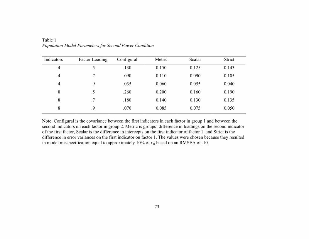
73
Table 1 Population Model Parameters for Second Power Condition
Note: Configural is the covariance between the first indicators in each factor in group 1 and between the second indicators on each factor in group 2. Metric is groups’ difference in loadings on the second indicator of the first factor, Scalar is the difference in intercepts on the first indicator of factor 1, and Strict is the difference in error variances on the first indicator on factor 1. The values were chosen because they resulted in model misspecification equal to approximately 10% of 𝜀! based on an RMSEA of .10.
Indicators Factor Loading Configural Metric Scalar Strict
4 .5 .130 0.150 0.125 0.143
4 .7 .090 0.110 0.090 0.105
4 .9 .035 0.060 0.055 0.040
8 .5 .260 0.200 0.160 0.190
8 .7 .180 0.140 0.130 0.135
8 .9 .070 0.085 0.075 0.050

74
Table 2 Population Model Parameters for Type I Error Conditions
Note: Configural is the covariance between the first indicators in each factor in group 1 and between the second indicators on each factor in group 2. Metric1 is the group difference in loadings on the second indicator of the first factor, Scalar1 is the difference in intercept on the first indicator of factor 1, and Strict1 is difference in error variance on the first indicator on factor 1 If metric, scalar, or strict are followed by 25 it represents the differences between the groups’ loading, intercept or error variance on 25% of the indicators .
Indicators Loadings RMSEA0 Configural Metric1 Metric25 Scalar1 Scalar25 Strict1 Strict25
4 .5 .05 .1900 0.2370 0.2130 0.1737 0.1506 0.2149 0.1560
4 .5 .08 .3010 0.3660 0.3382 0.2788 0.2445 0.3190 0.2365
4 .5 .10 .3720 0.4549 0.4222 0.3490 0.3100 0.3800 0.2848
4 .7 .05 .1362 0.1680 0.1436 0.1420 0.1250 0.1550 0.1105
4 .7 .08 .2122 0.2620 0.2285 0.2309 0.2000 0.2292 0.1658
4 .7 .10 .2600 0.3251 0.2830 0.2875 0.2500 0.2750 0.2000
4 .9 .05 .0532 0.1590 0.1375 0.0874 0.0755 0.0615 0.0425
4 .9 .08 .0835 0.2499 0.2154 0.1400 0.1211 0.0904 0.0641
4 .9 .10 .1025 0.3100 0.2677 0.1770 0.1510 0.1075 0.0765
8 .5 .05 .3887 0.2849 0.1846 0.2450 0.1645 0.2720 0.1465
8 .5 .08 .5650 0.4545 0.2910 0.3970 0.2650 0.3908 0.2215
8 .5 .10 .6500 0.5659 0.3600 0.4955 0.3300 0.4570 0.2676
8 .7 .05 .2705 0.2150 0.1385 0.2060 0.1340 0.1900 0.1015
8 .7 .08 .3945 0.3405 0.2179 0.3255 0.2150 0.2726 0.1525
8 .7 .10 .4547 0.4300 0.2690 0.4100 0.2680 0.3175 0.1825
8 .9 .05 .1028 0.1250 0.0810 0.1250 0.0820 0.0710 0.0380
8 .9 .08 .1497 0.2000 0.1288 0.1990 0.1300 0.1026 0.0570
8 .9 .10 .1729 0.2510 0.1601 0.2508 0.1650 0.1200 0.0685

75
Table 3 Type I Error Rates for Group 1 Model Fit (4 indicator model) Loadings RMSEA0 𝑛 TCS EQ EQ-A CFI95 MNCI95 RA05 RA08 RA10
.5 .05 100 0.812 0.058 0.523 0.484 0.786 0.528 - -
.05 250 0.495 0.044 0.537 0.401 0.916 0.528 - -
.05 500 0.151 0.060 0.566 0.377 0.983 0.555 - -
.05 1000 0.001 0.050 0.527 0.280 0.999 0.525 - -
.05 2000 0.000 0.048 0.496 0.168 1.000 0.530 - -
.08 100 0.516 0.059 0.580 0.218 0.475 0.245 0.565 -
.08 250 0.054 0.055 0.535 0.047 0.355 0.061 0.506 -
.08 500 0.000 0.059 0.593 0.003 0.331 0.008 0.577 -
.08 1000 0.000 0.046 0.481 0.000 0.202 0.000 0.502 -
.08 2000 0.000 0.048 0.407 0.000 0.103 0.000 0.510 -
.10 100 0.292 0.073 0.636 0.097 0.260 0.108 0.338 0.614
.10 250 0.006 0.075 0.645 0.005 0.086 0.007 0.152 0.620
.10 500 0.000 0.074 0.571 0.000 0.015 0.000 0.067 0.560
.10 1000 0.000 0.073 0.525 0.000 0.000 0.000 0.010 0.561
.10 2000 0.000 0.053 0.390 0.000 0.000 0.000 0.000 0.541
.7 .05 100 0.799 0.037 0.485 0.834 0.772 0.489 - -
.05 250 0.470 0.053 0.515 0.969 0.905 0.505 - -
.05 500 0.125 0.046 0.533 1.000 0.986 0.519 - -
.05 1000 0.003 0.053 0.534 1.000 0.999 0.528 - -
.05 2000 0.000 0.040 0.460 1.000 1.000 0.494 - -
.08 100 0.442 0.037 0.509 0.519 0.412 0.190 0.492 -

76
.08 250 0.046 0.046 0.552 0.576 0.375 0.052 0.531 -
.08 500 0.000 0.051 0.545 0.577 0.288 0.005 0.537 -
.08 1000 0.000 0.052 0.533 0.651 0.211 0.000 0.555 -
.08 2000 0.000 0.053 0.388 0.673 0.115 0.000 0.525 -
.10 100 0.232 0.049 0.526 0.301 0.205 0.069 0.265 0.499
.10 250 0.000 0.052 0.556 0.172 0.064 0.001 0.131 0.521
.10 500 0.000 0.051 0.546 0.060 0.010 0.000 0.034 0.537
.10 1000 0.000 0.050 0.502 0.011 0.000 0.000 0.002 0.532
.10 2000 0.000 0.053 0.348 0.002 0.000 0.000 0.000 0.517
.9 .05 100 0.762 0.051 0.491 1.000 0.735 0.496 - -
.05 250 0.479 0.044 0.525 1.000 0.907 0.516 - -
.05 500 0.123 0.040 0.537 1.000 0.977 0.527 - -
.05 1000 0.003 0.059 0.544 1.000 0.998 0.541 - -
.05 2000 0.000 0.045 0.477 1.000 1.000 0.511 - -
.08 100 0.437 0.050 0.491 0.990 0.403 0.182 0.480 -
.08 250 0.048 0.051 0.564 1.000 0.386 0.056 0.532 -
.08 500 0.000 0.044 0.567 1.000 0.293 0.006 0.553 -
.08 1000 0.000 0.045 0.490 1.000 0.192 0.000 0.510 -
.08 2000 0.000 0.053 0.391 1.000 0.117 0.000 0.512 -
.10 100 0.201 0.034 0.516 0.947 0.178 0.059 0.236 0.495
.10 250 0.002 0.042 0.525 1.000 0.049 0.003 0.095 0.503
.10 500 0.000 0.044 0.533 1.000 0.006 0.000 0.037 0.516
.10 1000 0.000 0.041 0.482 1.000 0.000 0.000 0.003 0.521
.10 2000 0.000 0.044 0.354 1.000 0.000 0.000 0.000 0.519
Note: n is sample size per group; TCS is the traditional 𝜒!, EQ is the unadjusted equivalence test, and EQ-A is the EQ with the adjustment

77
Table 4 Type I Error Rates for Group 2 Model Fit (4 indicator model) Loadings RMSEA0 𝑛 TCS EQ EQ-A CFI95 MNCI95 RA05 RA08 RA10
.5 .05 100 0.818 0.051 0.520 0.484 0.786 0.523 - -
.05 250 0.501 0.056 0.542 0.430 0.912 0.536 - -
.05 500 0.140 0.052 0.554 0.379 0.979 0.540 - -
.05 1000 0.001 0.065 0.566 0.295 0.999 0.563 - -
.05 2000 0.000 0.042 0.506 0.165 1.000 0.547 - -
.08 100 0.480 0.041 0.532 0.174 0.435 0.195 0.521 -
.08 250 0.048 0.048 0.550 0.036 0.382 0.055 0.524 -
.08 500 0.001 0.053 0.571 0.005 0.322 0.006 0.550 -
.08 1000 0.000 0.056 0.494 0.000 0.205 0.000 0.510 -
.08 2000 0.000 0.050 0.417 0.000 0.120 0.000 0.515 -
.10 100 0.280 0.058 0.595 0.076 0.244 0.090 0.311 0.568
.10 250 0.004 0.071 0.612 0.004 0.092 0.006 0.164 0.585
.10 500 0.000 0.068 0.577 0.000 0.018 0.000 0.057 0.565
.10 1000 0.000 0.074 0.508 0.000 0.002 0.000 0.008 0.537
.10 2000 0.000 0.058 0.408 0.000 0.000 0.000 0.000 0.574
.7 .05 100 0.755 0.048 0.476 0.805 0.732 0.481 - -
.05 250 0.490 0.037 0.524 0.970 0.920 0.517 - -
.05 500 0.113 0.044 0.535 0.997 0.985 0.526 - -
.05 1000 0.001 0.038 0.514 1.000 0.999 0.511 - -
.05 2000 0.000 0.045 0.469 1.000 1.000 0.502 - -
.08 100 0.440 0.033 0.491 0.518 0.410 0.188 0.482 -

78
.08 250 0.053 0.053 0.511 0.540 0.356 0.062 0.492 -
.08 500 0.000 0.043 0.530 0.588 0.298 0.001 0.513 -
.08 1000 0.000 0.039 0.488 0.596 0.196 0.000 0.503 -
.08 2000 0.000 0.044 0.383 0.643 0.103 0.000 0.510 -
.10 100 0.194 0.040 0.506 0.252 0.175 0.058 0.228 0.493
.10 250 0.003 0.042 0.550 0.157 0.053 0.004 0.128 0.521
.10 500 0.000 0.041 0.532 0.055 0.006 0.000 0.031 0.523
.10 1000 0.000 0.041 0.472 0.012 0.001 0.000 0.007 0.499
.10 2000 0.000 0.047 0.358 0.000 0.000 0.000 0.000 0.537
.9 .05 100 0.792 0.040 0.499 1.000 0.759 0.500 - -
.05 250 0.486 0.045 0.522 1.000 0.921 0.510 - -
.05 500 0.119 0.049 0.533 1.000 0.986 0.518 - -
.05 1000 0.004 0.058 0.553 1.000 0.998 0.550 - -
.05 2000 0.000 0.041 0.476 1.000 1.000 0.511 - -
.08 100 0.438 0.038 0.498 0.990 0.410 0.197 0.481 -
.08 250 0.042 0.042 0.541 1.000 0.355 0.049 0.516 -
.08 500 0.000 0.048 0.556 1.000 0.303 0.005 0.527 -
.08 1000 0.000 0.041 0.464 1.000 0.176 0.000 0.486 -
.08 2000 0.000 0.047 0.388 1.000 0.104 0.000 0.523 -
.10 100 0.209 0.042 0.507 0.957 0.181 0.061 0.239 0.483
.10 250 0.001 0.042 0.570 1.000 0.057 0.001 0.107 0.545
.10 500 0.000 0.045 0.534 1.000 0.007 0.000 0.027 0.527
.10 1000 0.000 0.041 0.454 1.000 0.000 0.000 0.002 0.494
.10 2000 0.000 0.044 0.346 1.000 0.000 0.000 0.000 0.513
Note: n is sample size per group; TCS is the traditional 𝜒!, EQ is the unadjusted equivalence test, and EQ-A is the EQ with the adjustment
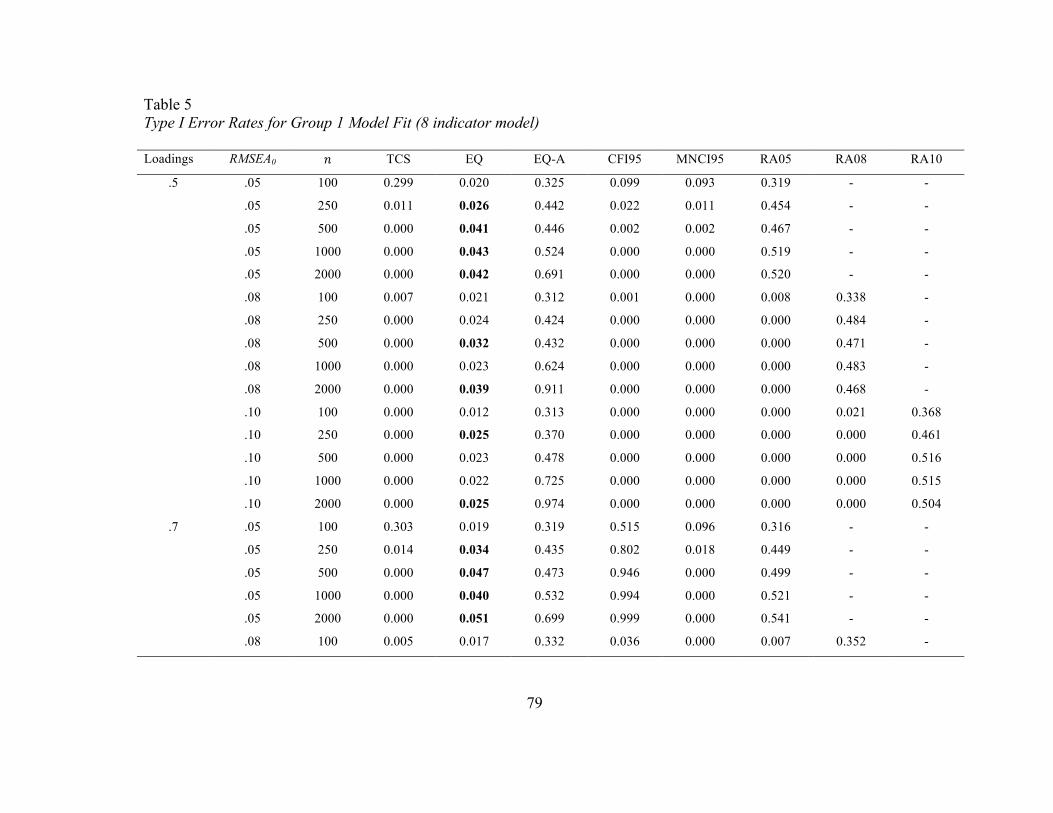
79
Table 5 Type I Error Rates for Group 1 Model Fit (8 indicator model) Loadings RMSEA0 𝑛 TCS EQ EQ-A CFI95 MNCI95 RA05 RA08 RA10
.5 .05 100 0.299 0.020 0.325 0.099 0.093 0.319 - -
.05 250 0.011 0.026 0.442 0.022 0.011 0.454 - -
.05 500 0.000 0.041 0.446 0.002 0.002 0.467 - -
.05 1000 0.000 0.043 0.524 0.000 0.000 0.519 - -
.05 2000 0.000 0.042 0.691 0.000 0.000 0.520 - -
.08 100 0.007 0.021 0.312 0.001 0.000 0.008 0.338 -
.08 250 0.000 0.024 0.424 0.000 0.000 0.000 0.484 -
.08 500 0.000 0.032 0.432 0.000 0.000 0.000 0.471 -
.08 1000 0.000 0.023 0.624 0.000 0.000 0.000 0.483 -
.08 2000 0.000 0.039 0.911 0.000 0.000 0.000 0.468 -
.10 100 0.000 0.012 0.313 0.000 0.000 0.000 0.021 0.368
.10 250 0.000 0.025 0.370 0.000 0.000 0.000 0.000 0.461
.10 500 0.000 0.023 0.478 0.000 0.000 0.000 0.000 0.516
.10 1000 0.000 0.022 0.725 0.000 0.000 0.000 0.000 0.515
.10 2000 0.000 0.025 0.974 0.000 0.000 0.000 0.000 0.504
.7 .05 100 0.303 0.019 0.319 0.515 0.096 0.316 - -
.05 250 0.014 0.034 0.435 0.802 0.018 0.449 - -
.05 500 0.000 0.047 0.473 0.946 0.000 0.499 - -
.05 1000 0.000 0.040 0.532 0.994 0.000 0.521 - -
.05 2000 0.000 0.051 0.699 0.999 0.000 0.541 - -
.08 100 0.005 0.017 0.332 0.036 0.000 0.007 0.352 -

80
.08 250 0.000 0.019 0.368 0.000 0.000 0.000 0.435 -
.08 500 0.000 0.021 0.417 0.000 0.000 0.000 0.462 -
.08 1000 0.000 0.030 0.624 0.000 0.000 0.000 0.478 -
.08 2000 0.000 0.038 0.901 0.000 0.000 0.000 0.506 -
.10 100 0.000 0.018 0.329 0.001 0.000 0.000 0.026 0.386
.10 250 0.000 0.018 0.358 0.000 0.000 0.000 0.000 0.467
.10 500 0.000 0.019 0.457 0.000 0.000 0.000 0.000 0.499
.10 1000 0.000 0.021 0.720 0.000 0.000 0.000 0.000 0.519
.10 2000 0.000 0.022 0.973 0.000 0.000 0.000 0.000 0.532
.9 .05 100 0.301 0.013 0.328 1.000 0.073 0.324 - -
.05 250 0.020 0.033 0.440 1.000 0.021 0.455 - -
.05 500 0.000 0.036 0.455 1.000 0.000 0.489 - -
.05 1000 0.000 0.039 0.539 1.000 0.000 0.526 - -
.05 2000 0.000 0.046 0.664 1.000 0.000 0.512 - -
.08 100 0.009 0.020 0.337 0.906 0.000 0.009 0.365 -
.08 250 0.000 0.030 0.409 1.000 0.000 0.000 0.468 -
.08 500 0.000 0.027 0.456 1.000 0.000 0.000 0.494 -
.08 1000 0.000 0.032 0.665 1.000 0.000 0.000 0.542 -
.08 2000 0.000 0.026 0.918 1.000 0.000 0.000 0.525 -
.10 100 0.000 0.010 0.313 0.382 0.000 0.000 0.014 0.363
.10 250 0.000 0.014 0.357 0.484 0.000 0.000 0.001 0.462
.10 500 0.000 0.020 0.430 0.510 0.000 0.000 0.000 0.459
.10 1000 0.000 0.013 0.692 0.537 0.000 0.000 0.000 0.485
.10 2000 0.000 0.016 0.964 0.571 0.000 0.000 0.000 0.499
Note: n is sample size per group; TCS is the traditional 𝜒!, EQ is the unadjusted equivalence test, and EQ-A is the EQ with the adjustment

81
Table 6 Type I Error Rates for Group 2 Model Fit (8 indicator model) Loadings RMSEA0 𝑛 TCS EQ EQ-A CFI95 MNCI95 RA05 RA08 RA10
.5 .05 100 0.297 0.021 0.328 0.103 0.087 0.324 - -
.05 250 0.008 0.026 0.455 0.023 0.011 0.464 - -
.05 500 0.000 0.038 0.470 0.001 0.000 0.498 - -
.05 1000 0.000 0.039 0.537 0.000 0.000 0.526 - -
.05 2000 0.000 0.042 0.672 0.000 0.000 0.497 - -
.08 100 0.006 0.018 0.318 0.001 0.000 0.008 0.338 -
.08 250 0.000 0.021 0.402 0.000 0.000 0.000 0.471 -
.08 500 0.000 0.033 0.411 0.000 0.000 0.000 0.464 -
.08 1000 0.000 0.024 0.608 0.000 0.000 0.000 0.493 -
.08 2000 0.000 0.034 0.910 0.000 0.000 0.000 0.491 -
.10 100 0.000 0.009 0.335 0.000 0.000 0.000 0.014 0.389
.10 250 0.000 0.016 0.396 0.000 0.000 0.000 0.001 0.497
.10 500 0.000 0.022 0.463 0.000 0.000 0.000 0.000 0.512
.10 1000 0.000 0.024 0.730 0.000 0.000 0.000 0.000 0.517
.10 2000 0.000 0.029 0.968 0.000 0.000 0.000 0.000 0.578
.7 .05 100 0.299 0.013 0.324 0.504 0.090 0.321 - -
.05 250 0.014 0.027 0.404 0.791 0.014 0.417 - -
.05 500 0.000 0.039 0.438 0.941 0.000 0.468 - -
.05 1000 0.000 0.046 0.537 0.995 0.000 0.525 - -
.05 2000 0.000 0.048 0.700 1.000 0.000 0.532 - -
.08 100 0.004 0.013 0.329 0.022 0.000 0.006 0.351 -

82
.08 250 0.000 0.018 0.399 0.001 0.000 0.000 0.470 -
.08 500 0.000 0.020 0.431 0.000 0.000 0.000 0.477 -
.08 1000 0.000 0.027 0.626 0.000 0.000 0.000 0.499 -
.08 2000 0.000 0.026 0.900 0.000 0.000 0.000 0.494 -
.10 100 0.000 0.009 0.326 0.000 0.000 0.000 0.018 0.379
.10 250 0.000 0.018 0.368 0.000 0.000 0.000 0.001 0.465
.10 500 0.000 0.032 0.461 0.000 0.000 0.000 0.000 0.500
.10 1000 0.000 0.018 0.702 0.000 0.000 0.000 0.000 0.504
.10 2000 0.000 0.023 0.969 0.000 0.000 0.000 0.000 0.491
.9 .05 100 0.278 0.010 0.302 0.999 0.068 0.297 0.933 1.000
.05 250 0.012 0.025 0.422 1.000 0.015 0.429 - -
.05 500 0.000 0.038 0.470 1.000 0.000 0.492 - -
.05 1000 0.000 0.028 0.508 1.000 0.000 0.493 - -
.05 2000 0.000 0.047 0.675 1.000 0.000 0.526 - -
.08 100 0.004 0.011 0.289 0.894 0.001 0.006 0.318 -
.08 250 0.000 0.018 0.380 1.000 0.000 0.000 0.445 -
.08 500 0.000 0.025 0.441 1.000 0.000 0.000 0.478 -
.08 1000 0.000 0.027 0.636 1.000 0.000 0.000 0.520 -
.08 2000 0.000 0.023 0.906 1.000 0.000 0.000 0.482 -
.10 100 0.000 0.007 0.289 0.363 0.000 0.000 0.010 0.331
.10 250 0.000 0.017 0.358 0.484 0.000 0.000 0.000 0.461
.10 500 0.000 0.020 0.439 0.511 0.000 0.000 0.000 0.476
.10 1000 0.000 0.019 0.729 0.586 0.000 0.000 0.000 0.522
.10 2000 0.000 0.023 0.967 0.551 0.000 0.000 0.000 0.472
Note: n is sample size per group; TCS is the traditional 𝜒!, EQ is the unadjusted equivalence test, and EQ-A is the EQ with the adjustment
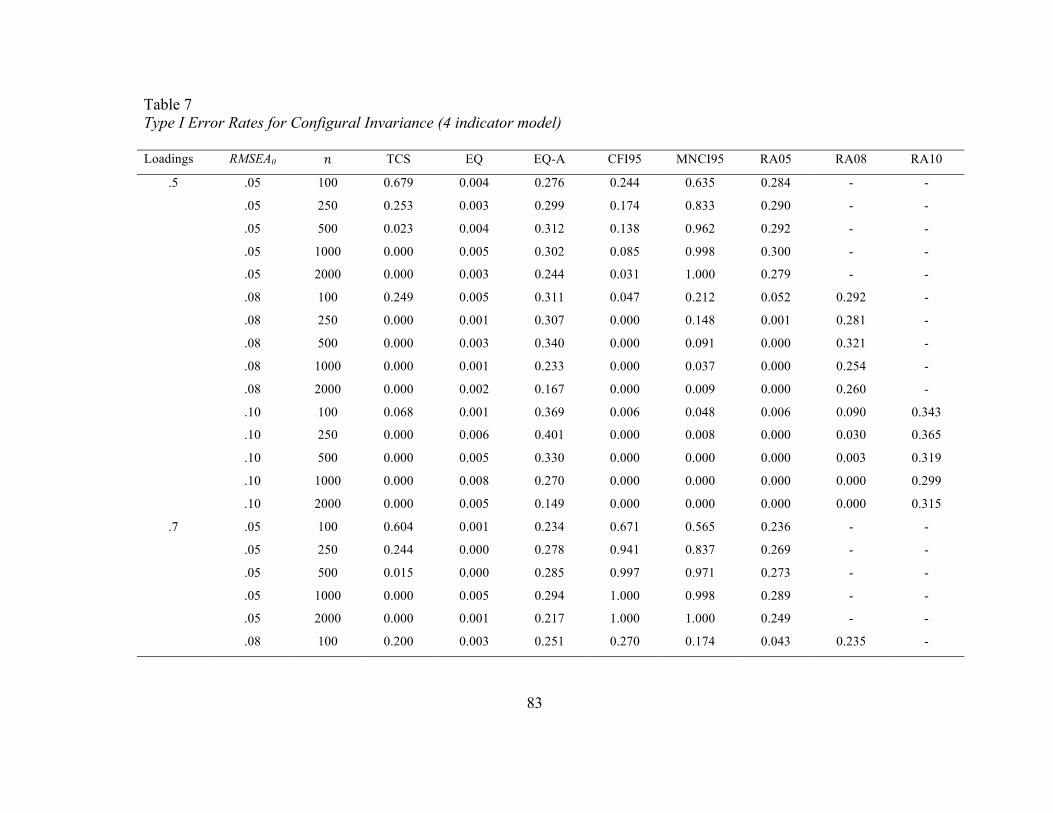
83
Table 7 Type I Error Rates for Configural Invariance (4 indicator model) Loadings RMSEA0 𝑛 TCS EQ EQ-A CFI95 MNCI95 RA05 RA08 RA10
.5 .05 100 0.679 0.004 0.276 0.244 0.635 0.284 - -
.05 250 0.253 0.003 0.299 0.174 0.833 0.290 - -
.05 500 0.023 0.004 0.312 0.138 0.962 0.292 - -
.05 1000 0.000 0.005 0.302 0.085 0.998 0.300 - -
.05 2000 0.000 0.003 0.244 0.031 1.000 0.279 - -
.08 100 0.249 0.005 0.311 0.047 0.212 0.052 0.292 -
.08 250 0.000 0.001 0.307 0.000 0.148 0.001 0.281 -
.08 500 0.000 0.003 0.340 0.000 0.091 0.000 0.321 -
.08 1000 0.000 0.001 0.233 0.000 0.037 0.000 0.254 -
.08 2000 0.000 0.002 0.167 0.000 0.009 0.000 0.260 -
.10 100 0.068 0.001 0.369 0.006 0.048 0.006 0.090 0.343
.10 250 0.000 0.006 0.401 0.000 0.008 0.000 0.030 0.365
.10 500 0.000 0.005 0.330 0.000 0.000 0.000 0.003 0.319
.10 1000 0.000 0.008 0.270 0.000 0.000 0.000 0.000 0.299
.10 2000 0.000 0.005 0.149 0.000 0.000 0.000 0.000 0.315
.7 .05 100 0.604 0.001 0.234 0.671 0.565 0.236 - -
.05 250 0.244 0.000 0.278 0.941 0.837 0.269 - -
.05 500 0.015 0.000 0.285 0.997 0.971 0.273 - -
.05 1000 0.000 0.005 0.294 1.000 0.998 0.289 - -
.05 2000 0.000 0.001 0.217 1.000 1.000 0.249 - -
.08 100 0.200 0.003 0.251 0.270 0.174 0.043 0.235 -

84
.08 250 0.003 0.003 0.289 0.318 0.127 0.005 0.263 -
.08 500 0.000 0.001 0.278 0.340 0.083 0.000 0.265 -
.08 1000 0.000 0.002 0.279 0.397 0.046 0.000 0.298 -
.08 2000 0.000 0.003 0.145 0.436 0.014 0.000 0.263 -
.10 100 0.046 0.000 0.258 0.075 0.034 0.002 0.061 0.244
.10 250 0.000 0.003 0.307 0.029 0.005 0.000 0.023 0.279
.10 500 0.000 0.003 0.281 0.005 0.000 0.000 0.003 0.275
.10 1000 0.000 0.002 0.245 0.000 0.000 0.000 0.000 0.272
.10 2000 0.000 0.002 0.122 0.000 0.000 0.000 0.000 0.275
.9 .05 100 0.595 0.003 0.247 1.000 0.553 0.250 - -
.05 250 0.244 0.002 0.281 1.000 0.835 0.269 - -
.05 500 0.019 0.005 0.281 1.000 0.963 0.264 - -
.05 1000 0.000 0.002 0.293 1.000 0.996 0.292 - -
.05 2000 0.000 0.000 0.219 1.000 1.000 0.254 - -
.08 100 0.206 0.006 0.265 0.980 0.172 0.032 0.256 -
.08 250 0.002 0.002 0.305 1.000 0.129 0.003 0.276 -
.08 500 0.000 0.001 0.321 1.000 0.082 0.000 0.297 -
.08 1000 0.000 0.000 0.232 1.000 0.031 0.000 0.253 -
.08 2000 0.000 0.003 0.153 1.000 0.009 0.000 0.272 -
.10 100 0.046 0.002 0.264 0.907 0.033 0.006 0.060 0.239
.10 250 0.000 0.001 0.296 1.000 0.002 0.000 0.011 0.270
.10 500 0.000 0.001 0.278 1.000 0.000 0.000 0.001 0.266
.10 1000 0.000 0.000 0.221 1.000 0.000 0.000 0.000 0.256
.10 2000 0.000 0.001 0.128 1.000 0.000 0.000 0.000 0.259
Note: n is sample size per group; TCS is the traditional 𝜒!, EQ is the unadjusted equivalence test, and EQ-A is the EQ with the adjustment
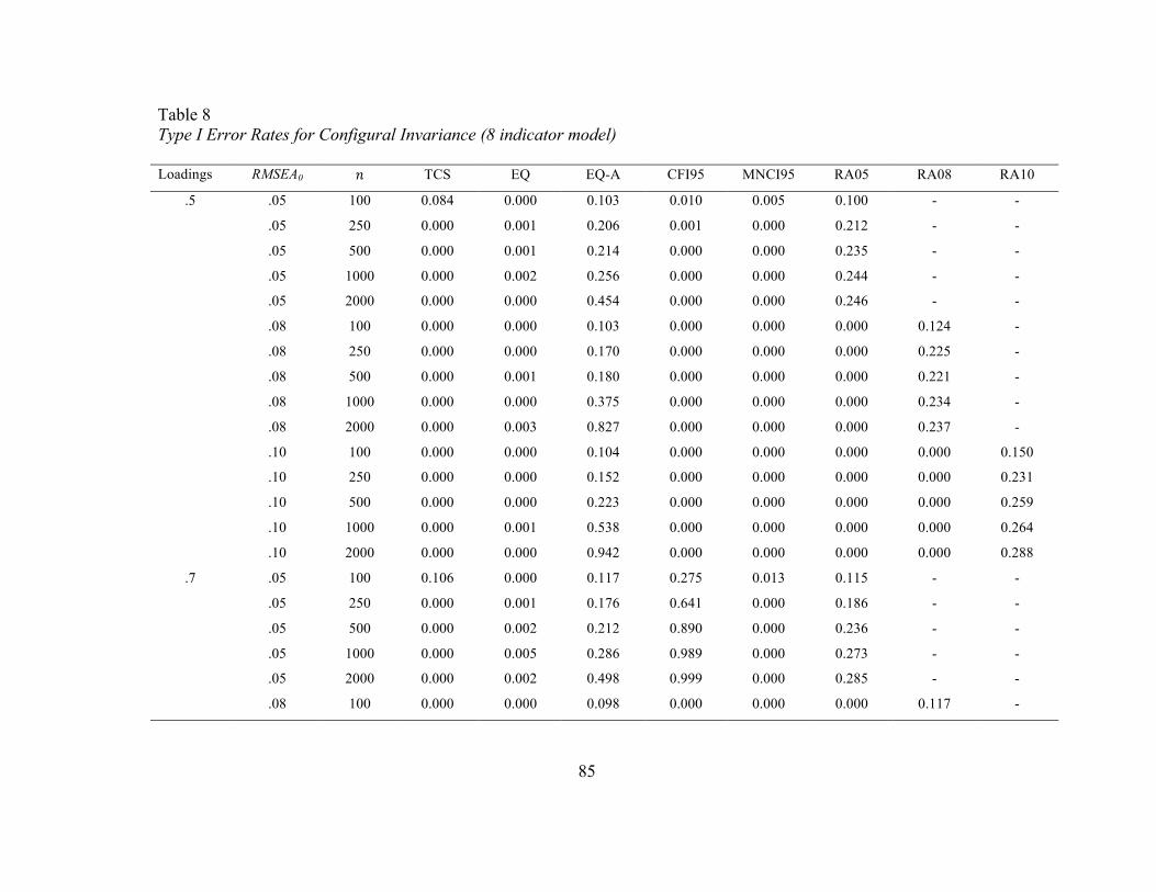
85
Table 8 Type I Error Rates for Configural Invariance (8 indicator model) Loadings RMSEA0 𝑛 TCS EQ EQ-A CFI95 MNCI95 RA05 RA08 RA10
.5 .05 100 0.084 0.000 0.103 0.010 0.005 0.100 - -
.05 250 0.000 0.001 0.206 0.001 0.000 0.212 - -
.05 500 0.000 0.001 0.214 0.000 0.000 0.235 - -
.05 1000 0.000 0.002 0.256 0.000 0.000 0.244 - -
.05 2000 0.000 0.000 0.454 0.000 0.000 0.246 - -
.08 100 0.000 0.000 0.103 0.000 0.000 0.000 0.124 -
.08 250 0.000 0.000 0.170 0.000 0.000 0.000 0.225 -
.08 500 0.000 0.001 0.180 0.000 0.000 0.000 0.221 -
.08 1000 0.000 0.000 0.375 0.000 0.000 0.000 0.234 -
.08 2000 0.000 0.003 0.827 0.000 0.000 0.000 0.237 -
.10 100 0.000 0.000 0.104 0.000 0.000 0.000 0.000 0.150
.10 250 0.000 0.000 0.152 0.000 0.000 0.000 0.000 0.231
.10 500 0.000 0.000 0.223 0.000 0.000 0.000 0.000 0.259
.10 1000 0.000 0.001 0.538 0.000 0.000 0.000 0.000 0.264
.10 2000 0.000 0.000 0.942 0.000 0.000 0.000 0.000 0.288
.7 .05 100 0.106 0.000 0.117 0.275 0.013 0.115 - -
.05 250 0.000 0.001 0.176 0.641 0.000 0.186 - -
.05 500 0.000 0.002 0.212 0.890 0.000 0.236 - -
.05 1000 0.000 0.005 0.286 0.989 0.000 0.273 - -
.05 2000 0.000 0.002 0.498 0.999 0.000 0.285 - -
.08 100 0.000 0.000 0.098 0.000 0.000 0.000 0.117 -

86
.08 250 0.000 0.001 0.153 0.000 0.000 0.000 0.199 -
.08 500 0.000 0.000 0.179 0.000 0.000 0.000 0.216 -
.08 1000 0.000 0.001 0.396 0.000 0.000 0.000 0.243 -
.08 2000 0.000 0.000 0.810 0.000 0.000 0.000 0.232 -
.10 100 0.000 0.000 0.105 0.000 0.000 0.000 0.000 0.148
.10 250 0.000 0.001 0.132 0.000 0.000 0.000 0.000 0.223
.10 500 0.000 0.000 0.210 0.000 0.000 0.000 0.000 0.247
.10 1000 0.000 0.000 0.510 0.000 0.000 0.000 0.000 0.267
.10 2000 0.000 0.000 0.942 0.000 0.000 0.000 0.000 0.268
.9 .05 100 0.078 0.000 0.088 0.999 0.005 0.084 - -
.05 250 0.000 0.000 0.205 1.000 0.000 0.214 - -
.05 500 0.000 0.000 0.218 1.000 0.000 0.248 - -
.05 1000 0.000 0.002 0.281 1.000 0.000 0.269 - -
.05 2000 0.000 0.002 0.443 1.000 0.000 0.271 - -
.08 100 0.000 0.000 0.106 0.811 0.000 0.000 0.126 -
.08 250 0.000 0.002 0.162 1.000 0.000 0.000 0.225 -
.08 500 0.000 0.000 0.191 1.000 0.000 0.000 0.225 -
.08 1000 0.000 0.000 0.424 1.000 0.000 0.000 0.284 -
.08 2000 0.000 0.001 0.833 1.000 0.000 0.000 0.243 -
.10 100 0.000 0.000 0.094 0.142 0.000 0.000 0.000 0.131
.10 250 0.000 0.001 0.120 0.244 0.000 0.000 0.000 0.214
.10 500 0.000 0.000 0.190 0.266 0.000 0.000 0.000 0.222
.10 1000 0.000 0.000 0.517 0.334 0.000 0.000 0.000 0.266
.10 2000 0.000 0.002 0.932 0.316 0.000 0.000 0.000 0.244
Note: n is sample size per group; TCS is the traditional 𝜒!, EQ is the unadjusted equivalence test, and EQ-A is the EQ with the adjustment

87
Table 9 Type I Error Rates for Metric Invariance (4 indicator model, Single noninvariant loading) Rel RMSEA0 𝑛 TCS EQ EQ-A ∆RMSEA ∆CFI ∆MNCI
.5 .05 100 0.859 0.047 0.522 0.695 0.453 0.69
.05 250 0.74 0.044 0.566 0.725 0.513 0.882
.05 500 0.512 0.052 0.577 0.648 0.469 0.958
.05 1000 0.171 0.053 0.581 0.488 0.313 0.994
.05 2000 0.008 0.055 0.596 0.252 0.13 1.00
.08 100 0.715 0.043 0.54 0.588 0.386 0.535
.08 250 0.407 0.056 0.611 0.447 0.283 0.605
.08 500 0.077 0.060 0.591 0.203 0.107 0.597
.08 1000 0.001 0.059 0.535 0.039 0.011 0.599
.08 2000 0 0.059 0.402 0.002 0 0.632
.10 100 0.58 0.048 0.556 0.478 0.296 0.399
.10 250 0.165 0.052 0.595 0.226 0.131 0.317
.10 500 0.007 0.05 0.572 0.038 0.019 0.199
.10 1000 0 0.047 0.478 0.001 0.001 0.093
.10 2000 0 0.046 0.277 0 0 0.027
.7 .05 100 0.869 0.045 0.539 0.685 0.654 0.701
.05 250 0.737 0.051 0.566 0.722 0.795 0.873
.05 500 0.491 0.046 0.559 0.636 0.837 0.953
.05 1000 0.146 0.044 0.563 0.464 0.889 0.996
.05 2000 0.005 0.049 0.577 0.23 0.937 0.999
.08 100 0.723 0.051 0.558 0.584 0.536 0.550
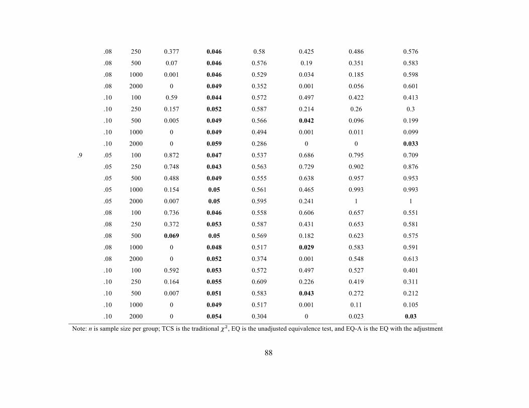
88
.08 250 0.377 0.046 0.58 0.425 0.486 0.576
.08 500 0.07 0.046 0.576 0.19 0.351 0.583
.08 1000 0.001 0.046 0.529 0.034 0.185 0.598
.08 2000 0 0.049 0.352 0.001 0.056 0.601
.10 100 0.59 0.044 0.572 0.497 0.422 0.413
.10 250 0.157 0.052 0.587 0.214 0.26 0.3
.10 500 0.005 0.049 0.566 0.042 0.096 0.199
.10 1000 0 0.049 0.494 0.001 0.011 0.099
.10 2000 0 0.059 0.286 0 0 0.033
.9 .05 100 0.872 0.047 0.537 0.686 0.795 0.709
.05 250 0.748 0.043 0.563 0.729 0.902 0.876
.05 500 0.488 0.049 0.555 0.638 0.957 0.953
.05 1000 0.154 0.05 0.561 0.465 0.993 0.993
.05 2000 0.007 0.05 0.595 0.241 1 1
.08 100 0.736 0.046 0.558 0.606 0.657 0.551
.08 250 0.372 0.053 0.587 0.431 0.653 0.581
.08 500 0.069 0.05 0.569 0.182 0.623 0.575
.08 1000 0 0.048 0.517 0.029 0.583 0.591
.08 2000 0 0.052 0.374 0.001 0.548 0.613
.10 100 0.592 0.053 0.572 0.497 0.527 0.401
.10 250 0.164 0.055 0.609 0.226 0.419 0.311
.10 500 0.007 0.051 0.583 0.043 0.272 0.212
.10 1000 0 0.049 0.517 0.001 0.11 0.105
.10 2000 0 0.054 0.304 0 0.023 0.03
Note: n is sample size per group; TCS is the traditional 𝜒!, EQ is the unadjusted equivalence test, and EQ-A is the EQ with the adjustment

89
Table 10 Type I Error Rates for Metric Invariance (8 indicator model, Single Noninvariant loading) Rel RMSEA0 𝑛 TCS EQ EQ-A ∆RMSEA ∆CFI ∆MNCI
.5 .05 100 0.826 0.042 0.516 0.901 0.39 0.475
.05 250 0.573 0.05 0.535 0.869 0.501 0.591
.05 500 0.224 0.053 0.531 0.81 0.439 0.624
.05 1000 0.014 0.048 0.539 0.73 0.316 0.69
.05 2000 0 0.047 0.563 0.559 0.139 0.729
.08 100 0.567 0.048 0.544 0.772 0.25 0.279
.08 250 0.11 0.051 0.547 0.533 0.174 0.122
.08 500 0.002 0.044 0.517 0.266 0.057 0.027
.08 1000 0 0.044 0.453 0.065 0.003 0.003
.08 2000 0 0.044 0.282 0.007 0 0
.10 100 0.325 0.043 0.54 0.606 0.142 0.116
.10 250 0.01 0.051 0.554 0.251 0.064 0.012
.10 500 0 0.052 0.527 0.046 0.007 0
.10 1000 0 0.05 0.434 0.001 0 0
.10 2000 0 0.049 0.215 0 0 0
.7 .05 100 0.816 0.042 0.522 0.896 0.72 0.474
.05 250 0.571 0.047 0.531 0.873 0.881 0.593
.05 500 0.212 0.047 0.54 0.822 0.948 0.627
.05 1000 0.011 0.044 0.519 0.726 0.988 0.672
.05 2000 0 0.046 0.553 0.55 1 0.722
.08 100 0.569 0.045 0.543 0.778 0.483 0.267

90
.08 250 0.111 0.053 0.568 0.55 0.464 0.121
.08 500 0.002 0.05 0.553 0.283 0.368 0.027
.08 1000 0 0.057 0.488 0.078 0.223 0.002
.08 2000 0 0.058 0.329 0.006 0.08 0
.10 100 0.325 0.046 0.54 0.615 0.297 0.126
.10 250 0.011 0.046 0.545 0.246 0.175 0.013
.10 500 0 0.049 0.512 0.047 0.061 0
.10 1000 0 0.044 0.428 0.001 0.003 0
.10 2000 0 0.043 0.200 0 0 0
.9 .05 100 0.829 0.052 0.541 0.897 0.986 0.486
.05 250 0.592 0.05 0.553 0.871 1 0.614
.05 500 0.225 0.05 0.545 0.829 1 0.638
.05 1000 0.01 0.05 0.537 0.73 1 0.683
.05 2000 0 0.047 0.561 0.558 1 0.729
.08 100 0.561 0.046 0.537 0.775 0.917 0.256
.08 250 0.112 0.046 0.563 0.551 0.988 0.123
.08 500 0.001 0.052 0.547 0.281 0.999 0.032
.08 1000 0 0.05 0.472 0.074 1 0.002
.08 2000 0 0.052 0.31 0.006 1 0
.10 100 0.336 0.047 0.542 0.626 0.783 0.121
.10 250 0.011 0.049 0.559 0.25 0.9 0.013
.10 500 0 0.049 0.523 0.045 0.959 0
.10 1000 0 0.048 0.432 0.001 0.991 0
.10 2000 0 0.049 0.219 0 1 0
Note: n is sample size per group; TCS is the traditional 𝜒!, EQ is the unadjusted equivalence test, and EQ-A is the EQ with the adjustment
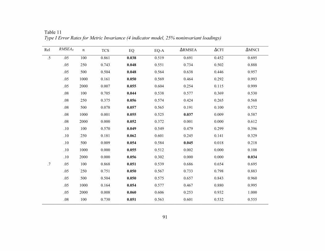
91
Table 11 Type I Error Rates for Metric Invariance (4 indicator model, 25% noninvariant loadings) Rel RMSEA0 𝑛 TCS EQ EQ-A ∆RMSEA ∆CFI ∆MNCI
.5 .05 100 0.861 0.038 0.519 0.691 0.452 0.695
.05 250 0.743 0.048 0.551 0.734 0.502 0.888
.05 500 0.504 0.048 0.564 0.638 0.446 0.957
.05 1000 0.161 0.050 0.569 0.464 0.292 0.993
.05 2000 0.007 0.055 0.604 0.254 0.115 0.999
.08 100 0.705 0.044 0.538 0.577 0.369 0.530
.08 250 0.375 0.056 0.574 0.424 0.265 0.568
.08 500 0.078 0.057 0.565 0.191 0.100 0.572
.08 1000 0.001 0.055 0.525 0.037 0.009 0.587
.08 2000 0.000 0.052 0.372 0.001 0.000 0.612
.10 100 0.570 0.049 0.549 0.479 0.299 0.396
.10 250 0.181 0.062 0.601 0.245 0.141 0.329
.10 500 0.009 0.054 0.584 0.045 0.018 0.218
.10 1000 0.000 0.055 0.512 0.002 0.000 0.108
.10 2000 0.000 0.056 0.302 0.000 0.000 0.034
.7 .05 100 0.868 0.051 0.539 0.686 0.654 0.695
.05 250 0.751 0.050 0.567 0.733 0.798 0.883
.05 500 0.504 0.050 0.575 0.657 0.843 0.960
.05 1000 0.164 0.054 0.577 0.467 0.880 0.995
.05 2000 0.008 0.060 0.606 0.253 0.932 1.000
.08 100 0.730 0.051 0.563 0.601 0.532 0.555
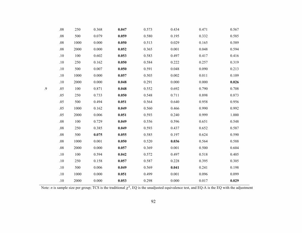
92
.08 250 0.368 0.047 0.573 0.434 0.471 0.567
.08 500 0.079 0.059 0.580 0.195 0.332 0.585
.08 1000 0.000 0.050 0.513 0.029 0.165 0.589
.08 2000 0.000 0.052 0.365 0.001 0.048 0.594
.10 100 0.602 0.053 0.583 0.497 0.417 0.416
.10 250 0.162 0.050 0.584 0.222 0.257 0.319
.10 500 0.007 0.050 0.591 0.048 0.090 0.213
.10 1000 0.000 0.057 0.503 0.002 0.011 0.109
.10 2000 0.000 0.048 0.291 0.000 0.000 0.026
.9 .05 100 0.871 0.048 0.552 0.692 0.790 0.708
.05 250 0.733 0.050 0.548 0.711 0.898 0.873
.05 500 0.494 0.051 0.564 0.640 0.958 0.956
.05 1000 0.162 0.049 0.560 0.466 0.990 0.992
.05 2000 0.006 0.051 0.593 0.240 0.999 1.000
.08 100 0.729 0.049 0.556 0.596 0.651 0.548
.08 250 0.385 0.049 0.593 0.437 0.652 0.587
.08 500 0.075 0.055 0.585 0.197 0.624 0.590
.08 1000 0.001 0.050 0.520 0.036 0.564 0.588
.08 2000 0.000 0.057 0.369 0.001 0.500 0.604
.10 100 0.594 0.042 0.572 0.497 0.518 0.405
.10 250 0.158 0.057 0.587 0.228 0.395 0.305
.10 500 0.006 0.049 0.569 0.041 0.241 0.198
.10 1000 0.000 0.051 0.499 0.001 0.096 0.099
.10 2000 0.000 0.053 0.298 0.000 0.017 0.029
Note: n is sample size per group; TCS is the traditional 𝜒!, EQ is the unadjusted equivalence test, and EQ-A is the EQ with the adjustment

93
Table 12 Type I Error Rates for Metric Invariance (8 indicator model, 25% Noninvariant loadings) Rel RMSEA0 𝑛 TCS EQ EQ-A ∆RMSEA ∆CFI ∆MNCI
.5 .05 100 0.802 0.041 0.501 0.888 0.368 0.452
.05 250 0.575 0.048 0.535 0.872 0.489 0.594
.05 500 0.232 0.047 0.549 0.824 0.437 0.647
.05 1000 0.013 0.055 0.535 0.714 0.302 0.681
.05 2000 0.000 0.055 0.575 0.566 0.125 0.735
.08 100 0.565 0.050 0.541 0.759 0.234 0.264
.08 250 0.112 0.050 0.547 0.523 0.171 0.123
.08 500 0.002 0.048 0.522 0.269 0.051 0.029
.08 1000 0.000 0.058 0.461 0.071 0.003 0.003
.08 2000 0.000 0.051 0.299 0.004 0.000 0.000
.10 100 0.340 0.050 0.541 0.607 0.142 0.125
.10 250 0.014 0.057 0.571 0.261 0.066 0.016
.10 500 0.000 0.062 0.529 0.052 0.003 0.000
.10 1000 0.000 0.062 0.427 0.001 0.000 0.000
.10 2000 0.000 0.054 0.220 0.000 0.000 0.000
.7 .05 100 0.813 0.045 0.526 0.895 0.710 0.487
.05 250 0.582 0.051 0.543 0.865 0.867 0.603
.05 500 0.234 0.049 0.542 0.812 0.940 0.631
.05 1000 0.011 0.051 0.537 0.713 0.986 0.677
.05 2000 0.000 0.056 0.571 0.569 0.998 0.731
.08 100 0.558 0.050 0.535 0.767 0.457 0.258
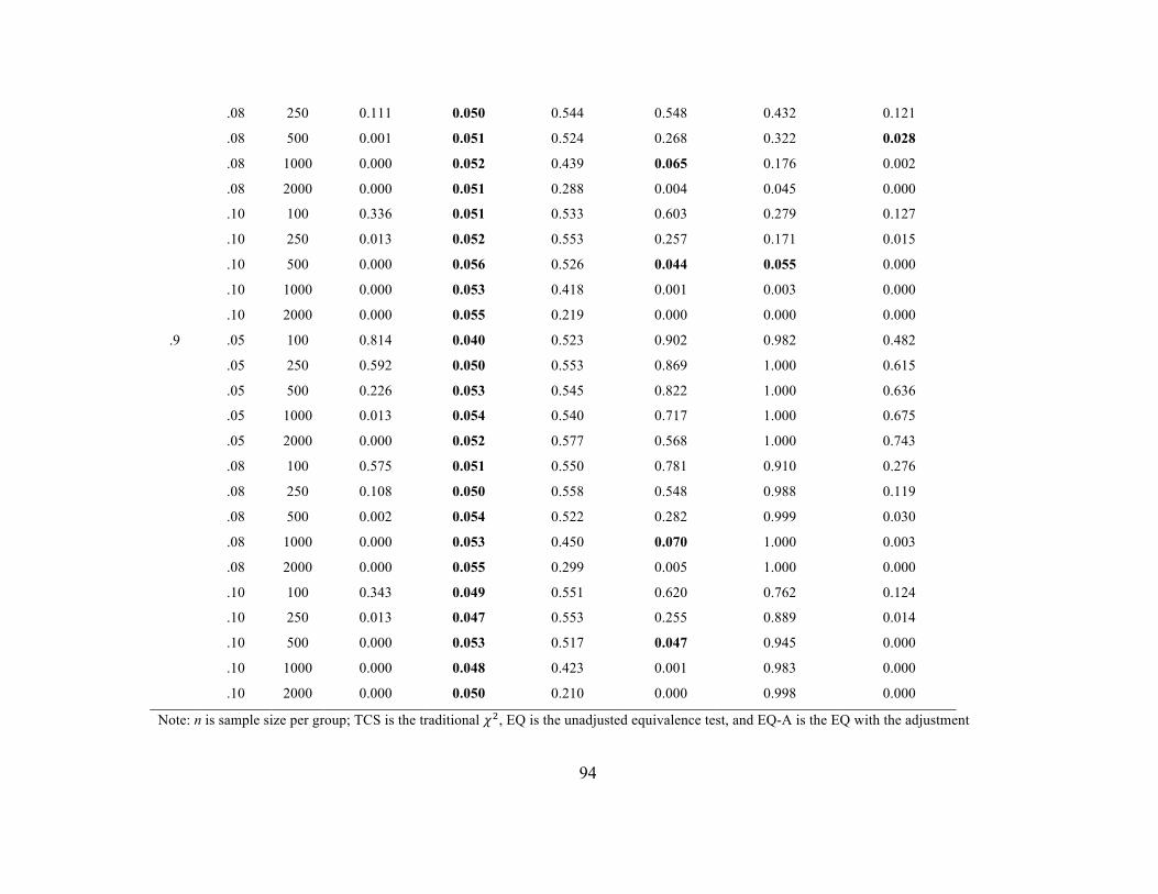
94
.08 250 0.111 0.050 0.544 0.548 0.432 0.121
.08 500 0.001 0.051 0.524 0.268 0.322 0.028
.08 1000 0.000 0.052 0.439 0.065 0.176 0.002
.08 2000 0.000 0.051 0.288 0.004 0.045 0.000
.10 100 0.336 0.051 0.533 0.603 0.279 0.127
.10 250 0.013 0.052 0.553 0.257 0.171 0.015
.10 500 0.000 0.056 0.526 0.044 0.055 0.000
.10 1000 0.000 0.053 0.418 0.001 0.003 0.000
.10 2000 0.000 0.055 0.219 0.000 0.000 0.000
.9 .05 100 0.814 0.040 0.523 0.902 0.982 0.482
.05 250 0.592 0.050 0.553 0.869 1.000 0.615
.05 500 0.226 0.053 0.545 0.822 1.000 0.636
.05 1000 0.013 0.054 0.540 0.717 1.000 0.675
.05 2000 0.000 0.052 0.577 0.568 1.000 0.743
.08 100 0.575 0.051 0.550 0.781 0.910 0.276
.08 250 0.108 0.050 0.558 0.548 0.988 0.119
.08 500 0.002 0.054 0.522 0.282 0.999 0.030
.08 1000 0.000 0.053 0.450 0.070 1.000 0.003
.08 2000 0.000 0.055 0.299 0.005 1.000 0.000
.10 100 0.343 0.049 0.551 0.620 0.762 0.124
.10 250 0.013 0.047 0.553 0.255 0.889 0.014
.10 500 0.000 0.053 0.517 0.047 0.945 0.000
.10 1000 0.000 0.048 0.423 0.001 0.983 0.000
.10 2000 0.000 0.050 0.210 0.000 0.998 0.000
Note: n is sample size per group; TCS is the traditional 𝜒!, EQ is the unadjusted equivalence test, and EQ-A is the EQ with the adjustment

95
Table 13 Type I Error Rates for Scalar Invariance (4 indicator model, Single noninvariant intercept) Rel RMSEA0 𝑛 TCS EQ EQ-A ∆RMSEA ∆CFI ∆MNCI
.5 .05 100 0.877 0.027 0.568 0.716 0.573 0.719
.05 250 0.757 0.059 0.566 0.752 0.553 0.890
.05 500 0.505 0.049 0.569 0.682 0.492 0.956
.05 1000 0.164 0.054 0.561 0.509 0.331 0.993
.05 2000 0.006 0.054 0.604 0.312 0.170 1.000
.08 100 0.752 0.058 0.582 0.634 0.473 0.569
.08 250 0.378 0.048 0.578 0.468 0.292 0.574
.08 500 0.077 0.059 0.568 0.223 0.117 0.580
.08 1000 0.001 0.055 0.517 0.045 0.014 0.590
.08 2000 0.000 0.055 0.364 0.002 0.000 0.603
.10 100 0.596 0.045 0.578 0.523 0.385 0.419
.10 250 0.157 0.052 0.596 0.251 0.153 0.307
.10 500 0.005 0.047 0.569 0.052 0.024 0.191
.10 1000 0.000 0.047 0.492 0.003 0.000 0.095
.10 2000 0.000 0.048 0.280 0.000 0.000 0.031
.7 .05 100 0.881 0.034 0.552 0.696 0.673 0.725
.05 250 0.754 0.055 0.579 0.760 0.808 0.890
.05 500 0.490 0.045 0.561 0.676 0.854 0.961
.05 1000 0.173 0.063 0.571 0.526 0.902 0.992
.05 2000 0.008 0.049 0.595 0.304 0.956 1.000
.08 100 0.735 0.048 0.556 0.621 0.555 0.551

96
.08 250 0.360 0.044 0.576 0.456 0.489 0.568
.08 500 0.071 0.052 0.566 0.210 0.366 0.569
.08 1000 0.001 0.051 0.505 0.045 0.219 0.584
.08 2000 0.000 0.045 0.346 0.001 0.071 0.577
.10 100 0.577 0.038 0.559 0.514 0.439 0.392
.10 250 0.146 0.040 0.576 0.234 0.269 0.295
.10 500 0.005 0.041 0.557 0.046 0.109 0.180
.10 1000 0.000 0.053 0.495 0.001 0.020 0.101
.10 2000 0.000 0.048 0.293 0.000 0.000 0.029
.9 .05 100 0.871 0.068 0.550 0.693 0.935 0.711
.05 250 0.728 0.050 0.555 0.750 0.993 0.883
.05 500 0.512 0.051 0.576 0.681 1.000 0.960
.05 1000 0.156 0.048 0.562 0.519 1.000 0.992
.05 2000 0.006 0.054 0.601 0.291 1.000 1.000
.08 100 0.727 0.036 0.563 0.612 0.847 0.548
.08 250 0.382 0.048 0.583 0.465 0.934 0.573
.08 500 0.071 0.049 0.573 0.228 0.980 0.582
.08 1000 0.001 0.049 0.532 0.044 0.997 0.601
.08 2000 0.000 0.050 0.371 0.003 1.000 0.609
.10 100 0.577 0.039 0.559 0.520 0.741 0.400
.10 250 0.154 0.043 0.572 0.254 0.786 0.308
.10 500 0.004 0.049 0.556 0.044 0.833 0.193
.10 1000 0.000 0.040 0.454 0.001 0.878 0.078
.10 2000 0.000 0.040 0.252 0.000 0.944 0.019
Note: n is sample size per group; TCS is the traditional 𝜒!, EQ is the unadjusted equivalence test, and EQ-A is the EQ with the adjustment

97
Table 14 Type I Error Rates for Scalar Invariance (8 indicator model, Single Noninvariant intercept) Rel RMSEA0 𝑛 TCS EQ EQ-A ∆RMSEA ∆CFI ∆MNCI
.5 .05 100 0.831 0.072 0.530 0.901 0.483 0.469
.05 250 0.573 0.047 0.529 0.877 0.524 0.595
.05 500 0.219 0.051 0.547 0.833 0.461 0.632
.05 1000 0.013 0.049 0.536 0.754 0.354 0.682
.05 2000 0.000 0.058 0.593 0.621 0.179 0.749
.08 100 0.559 0.044 0.539 0.778 0.321 0.261
.08 250 0.099 0.043 0.537 0.548 0.177 0.106
.08 500 0.002 0.039 0.514 0.294 0.063 0.022
.08 1000 0.000 0.042 0.450 0.080 0.007 0.001
.08 2000 0.000 0.035 0.265 0.008 0.000 0.000
.10 100 0.324 0.041 0.568 0.646 0.209 0.116
.10 250 0.011 0.048 0.561 0.270 0.072 0.011
.10 500 0.000 0.045 0.541 0.058 0.007 0.001
.10 1000 0.000 0.053 0.454 0.001 0.000 0.000
.10 2000 0.000 0.052 0.236 0.000 0.000 0.000
.7 .05 100 0.820 0.051 0.525 0.900 0.733 0.470
.05 250 0.569 0.043 0.530 0.875 0.886 0.585
.05 500 0.202 0.037 0.500 0.833 0.954 0.610
.05 1000 0.009 0.042 0.506 0.739 0.990 0.659
.05 2000 0.000 0.037 0.535 0.597 1.000 0.701
.08 100 0.550 0.038 0.516 0.787 0.483 0.249

98
.08 250 0.109 0.047 0.563 0.555 0.482 0.115
.08 500 0.003 0.050 0.532 0.303 0.387 0.027
.08 1000 0.000 0.048 0.484 0.101 0.252 0.002
.08 2000 0.000 0.048 0.313 0.006 0.102 0.000
.10 100 0.335 0.044 0.542 0.630 0.302 0.118
.10 250 0.011 0.046 0.549 0.282 0.191 0.014
.10 500 0.000 0.041 0.522 0.051 0.073 0.000
.10 1000 0.000 0.047 0.425 0.002 0.006 0.000
.10 2000 0.000 0.053 0.220 0.000 0.000 0.000
.9 .05 100 0.821 0.056 0.529 0.905 0.986 0.473
.05 250 0.566 0.042 0.526 0.879 1.000 0.586
.05 500 0.215 0.043 0.527 0.829 1.000 0.624
.05 1000 0.013 0.046 0.518 0.756 1.000 0.664
.05 2000 0.000 0.037 0.547 0.588 1.000 0.719
.08 100 0.567 0.040 0.536 0.788 0.912 0.261
.08 250 0.103 0.047 0.557 0.563 0.987 0.117
.08 500 0.001 0.049 0.535 0.311 1.000 0.034
.08 1000 0.000 0.037 0.465 0.088 1.000 0.001
.08 2000 0.000 0.051 0.304 0.013 1.000 0.000
.10 100 0.334 0.042 0.540 0.640 0.797 0.113
.10 250 0.012 0.044 0.544 0.274 0.891 0.012
.10 500 0.000 0.041 0.513 0.054 0.964 0.000
.10 1000 0.000 0.045 0.431 0.002 0.992 0.000
.10 2000 0.000 0.048 0.208 0.000 0.999 0.000
Note: n is sample size per group; TCS is the traditional 𝜒!, EQ is the unadjusted equivalence test, and EQ-A is the EQ with the adjustment

99
Table 15 Type I Error Rates for Scalar Invariance (4 indicator model, 25% noninvariant intercepts) Rel RMSEA0 𝑛 TCS EQ EQ-A ∆RMSEA ∆CFI ∆MNCI
.5 .05 100 0.880 0.037 0.562 0.724 0.590 0.721
.05 250 0.741 0.057 0.563 0.750 0.538 0.878
.05 500 0.513 0.055 0.578 0.691 0.503 0.958
.05 1000 0.161 0.049 0.570 0.523 0.346 0.993
.05 2000 0.009 0.059 0.593 0.303 0.157 1.000
.08 100 0.730 0.050 0.567 0.633 0.471 0.559
.08 250 0.386 0.048 0.594 0.473 0.284 0.588
.08 500 0.072 0.049 0.568 0.217 0.118 0.572
.08 1000 0.001 0.051 0.524 0.043 0.012 0.590
.08 2000 0.000 0.044 0.372 0.002 0.000 0.613
.10 100 0.599 0.050 0.584 0.537 0.396 0.432
.10 250 0.147 0.043 0.589 0.245 0.147 0.307
.10 500 0.008 0.049 0.570 0.047 0.022 0.190
.10 1000 0.000 0.047 0.477 0.001 0.001 0.100
.10 2000 0.000 0.046 0.272 0.000 0.000 0.024
.7 .05 100 0.877 0.046 0.539 0.706 0.679 0.705
.05 250 0.734 0.043 0.561 0.749 0.793 0.875
.05 500 0.503 0.046 0.569 0.687 0.846 0.953
.05 1000 0.153 0.045 0.555 0.504 0.888 0.991
.05 2000 0.007 0.046 0.573 0.286 0.946 1.000
.08 100 0.745 0.053 0.572 0.630 0.564 0.561

100
.08 250 0.359 0.049 0.573 0.447 0.485 0.569
.08 500 0.067 0.050 0.550 0.217 0.369 0.564
.08 1000 0.000 0.046 0.511 0.039 0.211 0.583
.08 2000 0.000 0.050 0.357 0.002 0.076 0.575
.10 100 0.598 0.046 0.578 0.529 0.447 0.413
.10 250 0.152 0.046 0.582 0.245 0.274 0.302
.10 500 0.007 0.049 0.559 0.052 0.109 0.198
.10 1000 0.000 0.046 0.479 0.001 0.017 0.092
.10 2000 0.000 0.048 0.282 0.000 0.000 0.027
.9 .05 100 0.878 0.050 0.566 0.708 0.938 0.714
.05 250 0.732 0.057 0.547 0.747 0.994 0.872
.05 500 0.512 0.047 0.574 0.685 0.999 0.960
.05 1000 0.151 0.046 0.568 0.510 1.000 0.992
.05 2000 0.008 0.049 0.581 0.302 1.000 1.000
.08 100 0.732 0.044 0.556 0.630 0.852 0.548
.08 250 0.365 0.044 0.569 0.447 0.928 0.565
.08 500 0.068 0.048 0.583 0.227 0.981 0.588
.08 1000 0.001 0.054 0.514 0.043 0.998 0.585
.08 2000 0.000 0.042 0.354 0.001 1.000 0.593
.10 100 0.599 0.049 0.579 0.527 0.762 0.411
.10 250 0.159 0.045 0.591 0.252 0.800 0.308
.10 500 0.004 0.046 0.578 0.045 0.849 0.192
.10 1000 0.000 0.048 0.507 0.001 0.901 0.097
.10 2000 0.000 0.047 0.282 0.000 0.953 0.026
Note: n is sample size per group; TCS is the traditional 𝜒!, EQ is the unadjusted equivalence test, and EQ-A is the EQ with the adjustment

101
Table 16 Type I Error Rates for Scalar Invariance (8 indicator model, 25% Noninvariant intercepts) Rel RMSEA0 𝑛 TCS EQ EQ-A ∆RMSEA ∆CFI ∆MNCI
.5 .05 100 0.818 0.033 0.532 0.902 0.481 0.454
.05 250 0.584 0.044 0.543 0.885 0.530 0.606
.05 500 0.220 0.051 0.531 0.837 0.464 0.626
.05 1000 0.012 0.046 0.507 0.741 0.323 0.663
.05 2000 0.000 0.041 0.544 0.599 0.165 0.704
.08 100 0.564 0.040 0.530 0.784 0.315 0.249
.08 250 0.109 0.048 0.549 0.561 0.174 0.115
.08 500 0.001 0.041 0.507 0.296 0.059 0.024
.08 1000 0.000 0.043 0.433 0.087 0.003 0.001
.08 2000 0.000 0.043 0.260 0.006 0.000 0.000
.10 100 0.345 0.048 0.549 0.644 0.214 0.123
.10 250 0.016 0.057 0.574 0.287 0.080 0.016
.10 500 0.000 0.056 0.537 0.059 0.006 0.001
.10 1000 0.000 0.053 0.453 0.003 0.000 0.000
.10 2000 0.000 0.053 0.224 0.000 0.000 0.000
.7 .05 100 0.827 0.049 0.524 0.899 0.742 0.467
.05 250 0.568 0.047 0.529 0.880 0.882 0.593
.05 500 0.221 0.046 0.527 0.832 0.952 0.625
.05 1000 0.013 0.052 0.536 0.751 0.991 0.676
.05 2000 0.000 0.053 0.569 0.611 1.000 0.737
.08 100 0.565 0.050 0.531 0.787 0.493 0.254

102
.08 250 0.101 0.045 0.539 0.555 0.459 0.115
.08 500 0.001 0.051 0.520 0.295 0.375 0.031
.08 1000 0.000 0.044 0.449 0.087 0.224 0.001
.08 2000 0.000 0.045 0.289 0.008 0.095 0.000
.10 100 0.330 0.047 0.552 0.637 0.302 0.125
.10 250 0.013 0.050 0.568 0.279 0.194 0.016
.10 500 0.000 0.059 0.534 0.061 0.079 0.000
.10 1000 0.000 0.056 0.436 0.002 0.007 0.000
.10 2000 0.000 0.058 0.233 0.000 0.000 0.000
.9 .05 100 0.826 0.026 0.531 0.898 0.982 0.467
.05 250 0.577 0.044 0.531 0.884 1.000 0.597
.05 500 0.214 0.048 0.528 0.831 1.000 0.622
.05 1000 0.008 0.050 0.522 0.755 1.000 0.661
.05 2000 0.000 0.047 0.561 0.608 1.000 0.722
.08 100 0.580 0.045 0.565 0.796 0.915 0.266
.08 250 0.119 0.053 0.559 0.567 0.992 0.129
.08 500 0.000 0.053 0.566 0.315 0.999 0.030
.08 1000 0.000 0.051 0.466 0.087 1.000 0.002
.08 2000 0.000 0.061 0.329 0.011 1.000 0.000
.10 100 0.330 0.049 0.535 0.626 0.764 0.116
.10 250 0.012 0.043 0.531 0.252 0.889 0.011
.10 500 0.000 0.042 0.502 0.052 0.951 0.000
.10 1000 0.000 0.041 0.386 0.002 0.988 0.000
.10 2000 0.000 0.040 0.183 0.000 1.000 0.000
Note: n is sample size per group; TCS is the traditional 𝜒!, EQ is the unadjusted equivalence test, and EQ-A is the EQ with the adjustment
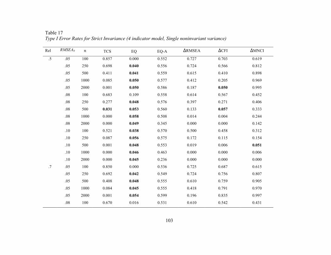
103
Table 17 Type I Error Rates for Strict Invariance (4 indicator model, Single noninvariant variance) Rel RMSEA0 𝑛 TCS EQ EQ-A ∆RMSEA ∆CFI ∆MNCI
.5 .05 100 0.857 0.000 0.552 0.727 0.703 0.619
.05 250 0.698 0.040 0.556 0.724 0.566 0.812
.05 500 0.411 0.041 0.559 0.615 0.410 0.898
.05 1000 0.085 0.050 0.577 0.412 0.205 0.969
.05 2000 0.001 0.050 0.586 0.187 0.050 0.995
.08 100 0.683 0.109 0.558 0.614 0.567 0.452
.08 250 0.277 0.048 0.576 0.397 0.271 0.406
.08 500 0.031 0.053 0.560 0.133 0.057 0.333
.08 1000 0.000 0.058 0.508 0.014 0.004 0.244
.08 2000 0.000 0.049 0.345 0.000 0.000 0.142
.10 100 0.521 0.038 0.570 0.500 0.458 0.312
.10 250 0.087 0.056 0.575 0.172 0.115 0.154
.10 500 0.001 0.048 0.553 0.019 0.006 0.051
.10 1000 0.000 0.046 0.463 0.000 0.000 0.006
.10 2000 0.000 0.045 0.236 0.000 0.000 0.000
.7 .05 100 0.850 0.000 0.536 0.725 0.687 0.615
.05 250 0.692 0.042 0.549 0.724 0.756 0.807
.05 500 0.408 0.048 0.555 0.610 0.759 0.905
.05 1000 0.084 0.045 0.555 0.418 0.791 0.970
.05 2000 0.001 0.054 0.599 0.196 0.835 0.997
.08 100 0.670 0.016 0.531 0.610 0.542 0.431
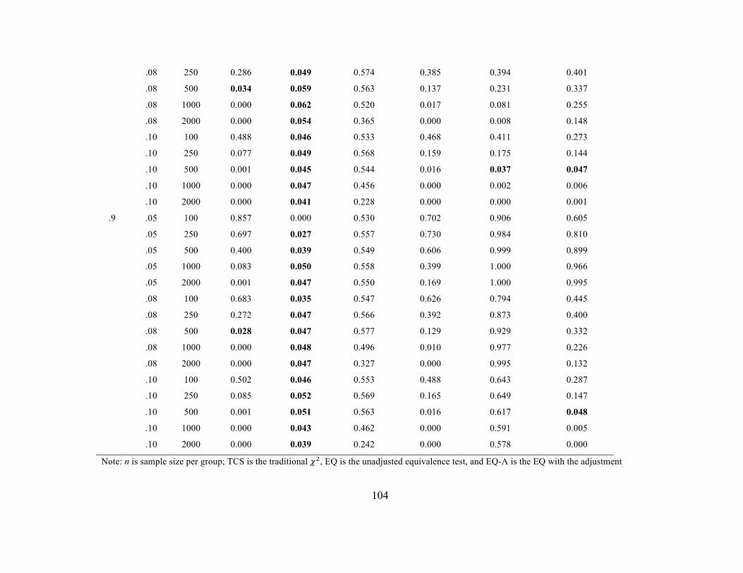
104
.08 250 0.286 0.049 0.574 0.385 0.394 0.401
.08 500 0.034 0.059 0.563 0.137 0.231 0.337
.08 1000 0.000 0.062 0.520 0.017 0.081 0.255
.08 2000 0.000 0.054 0.365 0.000 0.008 0.148
.10 100 0.488 0.046 0.533 0.468 0.411 0.273
.10 250 0.077 0.049 0.568 0.159 0.175 0.144
.10 500 0.001 0.045 0.544 0.016 0.037 0.047
.10 1000 0.000 0.047 0.456 0.000 0.002 0.006
.10 2000 0.000 0.041 0.228 0.000 0.000 0.001
.9 .05 100 0.857 0.000 0.530 0.702 0.906 0.605
.05 250 0.697 0.027 0.557 0.730 0.984 0.810
.05 500 0.400 0.039 0.549 0.606 0.999 0.899
.05 1000 0.083 0.050 0.558 0.399 1.000 0.966
.05 2000 0.001 0.047 0.550 0.169 1.000 0.995
.08 100 0.683 0.035 0.547 0.626 0.794 0.445
.08 250 0.272 0.047 0.566 0.392 0.873 0.400
.08 500 0.028 0.047 0.577 0.129 0.929 0.332
.08 1000 0.000 0.048 0.496 0.010 0.977 0.226
.08 2000 0.000 0.047 0.327 0.000 0.995 0.132
.10 100 0.502 0.046 0.553 0.488 0.643 0.287
.10 250 0.085 0.052 0.569 0.165 0.649 0.147
.10 500 0.001 0.051 0.563 0.016 0.617 0.048
.10 1000 0.000 0.043 0.462 0.000 0.591 0.005
.10 2000 0.000 0.039 0.242 0.000 0.578 0.000
Note: n is sample size per group; TCS is the traditional 𝜒!, EQ is the unadjusted equivalence test, and EQ-A is the EQ with the adjustment

105
Table 18 Type I Error Rates for Strict Invariance (8 indicator model, Single Noninvariant variance) Rel RMSEA0 𝑛 TCS EQ EQ-A ∆RMSEA ∆CFI ∆MNCI
.5 .05 100 0.797 0.028 0.502 0.897 0.581 0.415
.05 250 0.539 0.042 0.532 0.876 0.528 0.532
.05 500 0.175 0.049 0.542 0.815 0.412 0.543
.05 1000 0.003 0.050 0.537 0.713 0.263 0.540
.05 2000 0.000 0.045 0.544 0.532 0.093 0.506
.08 100 0.540 0.050 0.541 0.784 0.426 0.217
.08 250 0.078 0.053 0.542 0.511 0.179 0.076
.08 500 0.001 0.045 0.524 0.247 0.046 0.010
.08 1000 0.000 0.045 0.462 0.053 0.002 0.000
.08 2000 0.000 0.040 0.270 0.003 0.000 0.000
.10 100 0.272 0.042 0.520 0.610 0.285 0.079
.10 250 0.004 0.040 0.535 0.214 0.063 0.004
.10 500 0.000 0.044 0.513 0.028 0.003 0.000
.10 1000 0.000 0.042 0.396 0.000 0.000 0.000
.10 2000 0.000 0.037 0.178 0.000 0.000 0.000
.7 .05 100 0.793 0.000 0.491 0.888 0.698 0.394
.05 250 0.542 0.048 0.538 0.863 0.853 0.534
.05 500 0.166 0.041 0.530 0.816 0.932 0.527
.05 1000 0.006 0.049 0.506 0.695 0.977 0.518
.05 2000 0.000 0.035 0.534 0.521 0.997 0.498
.08 100 0.505 0.047 0.511 0.769 0.447 0.200
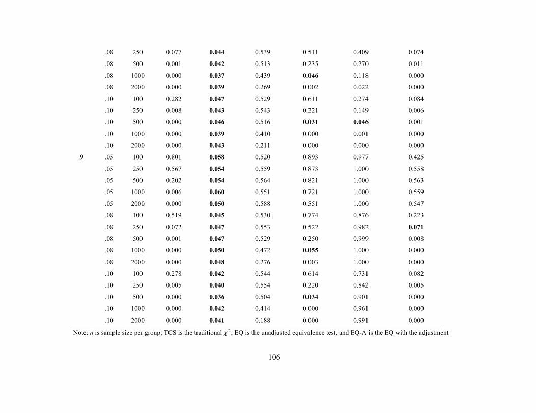
106
.08 250 0.077 0.044 0.539 0.511 0.409 0.074
.08 500 0.001 0.042 0.513 0.235 0.270 0.011
.08 1000 0.000 0.037 0.439 0.046 0.118 0.000
.08 2000 0.000 0.039 0.269 0.002 0.022 0.000
.10 100 0.282 0.047 0.529 0.611 0.274 0.084
.10 250 0.008 0.043 0.543 0.221 0.149 0.006
.10 500 0.000 0.046 0.516 0.031 0.046 0.001
.10 1000 0.000 0.039 0.410 0.000 0.001 0.000
.10 2000 0.000 0.043 0.211 0.000 0.000 0.000
.9 .05 100 0.801 0.058 0.520 0.893 0.977 0.425
.05 250 0.567 0.054 0.559 0.873 1.000 0.558
.05 500 0.202 0.054 0.564 0.821 1.000 0.563
.05 1000 0.006 0.060 0.551 0.721 1.000 0.559
.05 2000 0.000 0.050 0.588 0.551 1.000 0.547
.08 100 0.519 0.045 0.530 0.774 0.876 0.223
.08 250 0.072 0.047 0.553 0.522 0.982 0.071
.08 500 0.001 0.047 0.529 0.250 0.999 0.008
.08 1000 0.000 0.050 0.472 0.055 1.000 0.000
.08 2000 0.000 0.048 0.276 0.003 1.000 0.000
.10 100 0.278 0.042 0.544 0.614 0.731 0.082
.10 250 0.005 0.040 0.554 0.220 0.842 0.005
.10 500 0.000 0.036 0.504 0.034 0.901 0.000
.10 1000 0.000 0.042 0.414 0.000 0.961 0.000
.10 2000 0.000 0.041 0.188 0.000 0.991 0.000
Note: n is sample size per group; TCS is the traditional 𝜒!, EQ is the unadjusted equivalence test, and EQ-A is the EQ with the adjustment

107
Table 19 Type I Error Rates for Strict Invariance (4 indicator model, 25% noninvariant variances) Rel RMSEA0 𝑛 TCS EQ EQ-A ∆RMSEA ∆CFI ∆MNCI
.5 .05 100 0.854 0.000 0.539 0.728 0.694 0.620
.05 250 0.692 0.041 0.555 0.721 0.559 0.811
.05 500 0.427 0.044 0.569 0.621 0.436 0.911
.05 1000 0.094 0.053 0.588 0.416 0.228 0.974
.05 2000 0.001 0.058 0.610 0.204 0.063 0.997
.08 100 0.685 0.042 0.554 0.627 0.577 0.456
.08 250 0.282 0.063 0.574 0.401 0.292 0.405
.08 500 0.029 0.051 0.562 0.141 0.065 0.342
.08 1000 0.000 0.051 0.504 0.012 0.002 0.237
.08 2000 0.000 0.049 0.343 0.001 0.000 0.148
.10 100 0.506 0.048 0.556 0.482 0.444 0.284
.10 250 0.096 0.056 0.586 0.172 0.120 0.155
.10 500 0.001 0.050 0.570 0.018 0.008 0.053
.10 1000 0.000 0.053 0.477 0.000 0.000 0.007
.10 2000 0.000 0.048 0.269 0.000 0.000 0.000
.7 .05 100 0.856 0.000 0.544 0.748 0.701 0.617
.05 250 0.703 0.016 0.564 0.724 0.756 0.810
.05 500 0.414 0.050 0.563 0.622 0.778 0.910
.05 1000 0.080 0.046 0.567 0.414 0.794 0.973
.05 2000 0.001 0.053 0.596 0.188 0.839 0.995
.08 100 0.679 0.027 0.544 0.614 0.538 0.439

108
.08 250 0.291 0.058 0.575 0.396 0.391 0.413
.08 500 0.029 0.047 0.578 0.139 0.221 0.343
.08 1000 0.000 0.056 0.515 0.015 0.082 0.259
.08 2000 0.000 0.062 0.364 0.000 0.010 0.161
.10 100 0.514 0.037 0.559 0.495 0.421 0.292
.10 250 0.080 0.044 0.578 0.164 0.168 0.142
.10 500 0.000 0.051 0.548 0.017 0.040 0.055
.10 1000 0.000 0.052 0.465 0.000 0.002 0.007
.10 2000 0.000 0.045 0.248 0.000 0.000 0.000
.9 .05 100 0.863 0.000 0.539 0.730 0.910 0.627
.05 250 0.710 0.085 0.570 0.732 0.986 0.808
.05 500 0.414 0.054 0.566 0.614 0.999 0.906
.05 1000 0.081 0.044 0.547 0.380 1.000 0.961
.05 2000 0.001 0.045 0.591 0.187 1.000 0.996
.08 100 0.660 0.042 0.535 0.596 0.782 0.429
.08 250 0.274 0.046 0.560 0.387 0.866 0.393
.08 500 0.024 0.044 0.543 0.129 0.929 0.327
.08 1000 0.000 0.040 0.481 0.012 0.971 0.216
.08 2000 0.000 0.043 0.313 0.000 0.995 0.119
.10 100 0.500 0.038 0.542 0.495 0.666 0.295
.10 250 0.083 0.043 0.562 0.173 0.638 0.148
.10 500 0.000 0.048 0.557 0.018 0.628 0.051
.10 1000 0.000 0.051 0.463 0.000 0.599 0.007
.10 2000 0.000 0.042 0.242 0.000 0.574 0.000
Note: n is sample size per group; TCS is the traditional 𝜒!, EQ is the unadjusted equivalence test, and EQ-A is the EQ with the adjustment

109
Table 20 Type I Error Rates for Strict Invariance (8 indicator model, 25% Noninvariant variances) Rel RMSEA0 𝑛 TCS EQ EQ-A ∆RMSEA ∆CFI ∆MNCI
.5 .05 100 0.810 0.083 0.518 0.906 0.602 0.427
.05 250 0.578 0.062 0.575 0.882 0.547 0.563
.05 500 0.169 0.049 0.528 0.813 0.397 0.525
.05 1000 0.006 0.057 0.546 0.711 0.277 0.555
.05 2000 0.000 0.056 0.588 0.545 0.113 0.555
.08 100 0.529 0.029 0.532 0.793 0.427 0.258
.08 250 0.073 0.042 0.535 0.504 0.179 0.065
.08 500 0.000 0.038 0.507 0.241 0.051 0.006
.08 1000 0.000 0.053 0.446 0.053 0.001 0.001
.08 2000 0.000 0.053 0.306 0.003 0.000 0.000
.10 100 0.281 0.037 0.513 0.624 0.280 0.097
.10 250 0.005 0.046 0.524 0.225 0.064 0.007
.10 500 0.000 0.047 0.504 0.028 0.004 0.000
.10 1000 0.000 0.044 0.423 0.000 0.000 0.000
.10 2000 0.000 0.044 0.186 0.000 0.000 0.000
.7 .05 100 0.809 0.000 0.504 0.897 0.715 0.403
.05 250 0.549 0.052 0.535 0.860 0.856 0.533
.05 500 0.191 0.053 0.532 0.821 0.942 0.530
.05 1000 0.004 0.047 0.504 0.692 0.974 0.509
.05 2000 0.000 0.043 0.560 0.538 0.998 0.510
.08 100 0.503 0.046 0.519 0.782 0.449 0.185

110
.08 250 0.082 0.051 0.538 0.505 0.437 0.077
.08 500 0.000 0.040 0.549 0.226 0.305 0.008
.08 1000 0.000 0.046 0.437 0.052 0.136 0.001
.08 2000 0.000 0.051 0.281 0.002 0.028 0.000
.10 100 0.289 0.043 0.551 0.628 0.286 0.080
.10 250 0.004 0.051 0.563 0.247 0.151 0.005
.10 500 0.000 0.051 0.526 0.033 0.049 0.000
.10 1000 0.000 0.050 0.456 0.001 0.003 0.000
.10 2000 0.000 0.060 0.256 0.000 0.000 0.000
.9 .05 100 0.821 0.067 0.535 0.895 0.976 0.418
.05 250 0.546 0.044 0.547 0.868 1.000 0.535
.05 500 0.180 0.052 0.533 0.819 1.000 0.535
.05 1000 0.005 0.048 0.525 0.693 1.000 0.527
.05 2000 0.000 0.042 0.572 0.533 1.000 0.547
.08 100 0.508 0.045 0.529 0.770 0.877 0.203
.08 250 0.074 0.048 0.561 0.527 0.980 0.069
.08 500 0.001 0.049 0.525 0.246 1.000 0.012
.08 1000 0.000 0.051 0.438 0.052 1.000 0.000
.08 2000 0.000 0.045 0.310 0.005 1.000 0.000
.10 100 0.291 0.050 0.553 0.604 0.728 0.101
.10 250 0.010 0.055 0.551 0.228 0.855 0.009
.10 500 0.000 0.047 0.532 0.034 0.922 0.000
.10 1000 0.000 0.048 0.412 0.000 0.967 0.000
.10 2000 0.000 0.055 0.232 0.000 0.991 0.000
Note: n is sample size per group; TCS is the traditional 𝜒!, EQ is the unadjusted equivalence test, and EQ-A is the EQ with the adjustment
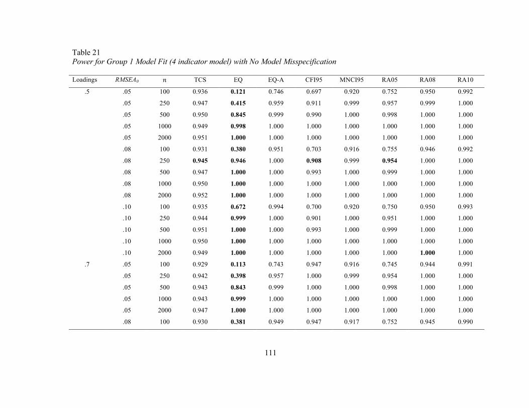
111
Table 21 Power for Group 1 Model Fit (4 indicator model) with No Model Misspecification Loadings RMSEA0 𝑛 TCS EQ EQ-A CFI95 MNCI95 RA05 RA08 RA10
.5 .05 100 0.936 0.121 0.746 0.697 0.920 0.752 0.950 0.992
.05 250 0.947 0.415 0.959 0.911 0.999 0.957 0.999 1.000
.05 500 0.950 0.845 0.999 0.990 1.000 0.998 1.000 1.000
.05 1000 0.949 0.998 1.000 1.000 1.000 1.000 1.000 1.000
.05 2000 0.951 1.000 1.000 1.000 1.000 1.000 1.000 1.000
.08 100 0.931 0.380 0.951 0.703 0.916 0.755 0.946 0.992
.08 250 0.945 0.946 1.000 0.908 0.999 0.954 1.000 1.000
.08 500 0.947 1.000 1.000 0.993 1.000 0.999 1.000 1.000
.08 1000 0.950 1.000 1.000 1.000 1.000 1.000 1.000 1.000
.08 2000 0.952 1.000 1.000 1.000 1.000 1.000 1.000 1.000
.10 100 0.935 0.672 0.994 0.700 0.920 0.750 0.950 0.993
.10 250 0.944 0.999 1.000 0.901 1.000 0.951 1.000 1.000
.10 500 0.951 1.000 1.000 0.993 1.000 0.999 1.000 1.000
.10 1000 0.950 1.000 1.000 1.000 1.000 1.000 1.000 1.000
.10 2000 0.949 1.000 1.000 1.000 1.000 1.000 1.000 1.000
.7 .05 100 0.929 0.113 0.743 0.947 0.916 0.745 0.944 0.991
.05 250 0.942 0.398 0.957 1.000 0.999 0.954 1.000 1.000
.05 500 0.943 0.843 0.999 1.000 1.000 0.998 1.000 1.000
.05 1000 0.943 0.999 1.000 1.000 1.000 1.000 1.000 1.000
.05 2000 0.947 1.000 1.000 1.000 1.000 1.000 1.000 1.000
.08 100 0.930 0.381 0.949 0.947 0.917 0.752 0.945 0.990

112
.08 250 0.939 0.940 1.000 1.000 1.000 0.948 1.000 1.000
.08 500 0.947 1.000 1.000 1.000 1.000 0.998 1.000 1.000
.08 1000 0.947 1.000 1.000 1.000 1.000 1.000 1.000 1.000
.08 2000 0.951 1.000 1.000 1.000 1.000 1.000 1.000 1.000
.10 100 0.929 0.654 0.989 0.944 0.914 0.744 0.941 0.987
.10 250 0.937 0.999 1.000 1.000 0.999 0.951 1.000 1.000
.10 500 0.949 1.000 1.000 1.000 1.000 0.998 1.000 1.000
.10 1000 0.948 1.000 1.000 1.000 1.000 1.000 1.000 1.000
.10 2000 0.953 1.000 1.000 1.000 1.000 1.000 1.000 1.000
.9 .05 100 0.922 0.111 0.731 1.000 0.908 0.736 0.939 0.988
.05 250 0.940 0.388 0.953 1.000 0.999 0.951 1.000 1.000
.05 500 0.944 0.846 0.998 1.000 1.000 0.998 1.000 1.000
.05 1000 0.947 0.999 1.000 1.000 1.000 1.000 1.000 1.000
.05 2000 0.953 1.000 1.000 1.000 1.000 1.000 1.000 1.000
.08 100 0.927 0.372 0.946 1.000 0.912 0.735 0.943 0.988
.08 250 0.935 0.936 1.000 1.000 0.999 0.945 1.000 1.000
.08 500 0.943 1.000 1.000 1.000 1.000 0.999 1.000 1.000
.08 1000 0.954 1.000 1.000 1.000 1.000 1.000 1.000 1.000
.08 2000 0.947 1.000 1.000 1.000 1.000 1.000 1.000 1.000
.10 100 0.931 0.654 0.992 1.000 0.915 0.740 0.944 0.990
.10 250 0.939 0.998 1.000 1.000 0.999 0.948 1.000 1.000
.10 500 0.949 1.000 1.000 1.000 1.000 0.999 1.000 1.000
.10 1000 0.950 1.000 1.000 1.000 1.000 1.000 1.000 1.000
.10 2000 0.949 1.000 1.000 1.000 1.000 1.000 1.000 1.000
Note: n is sample size per group; TCS is the traditional 𝜒!, EQ is the unadjusted equivalence test, and EQ-A is the EQ with the adjustment

113
Table 22 Power for Group 2 Model Fit (4 indicator model) with No Model Misspecification Loadings RMSEA0 𝑛 TCS EQ EQ-A CFI95 MNCI95 RA05 RA08 RA10
.5 .05 100 0.936 0.128 0.754 0.708 0.923 0.756 0.949 0.992
.05 250 0.941 0.396 0.954 0.902 0.999 0.951 1.000 1.000
.05 500 0.946 0.839 0.998 0.990 1.000 0.998 1.000 1.000
.05 1000 0.951 0.999 1.000 1.000 1.000 1.000 1.000 1.000
.05 2000 0.948 1.000 1.000 1.000 1.000 1.000 1.000 1.000
.08 100 0.930 0.384 0.950 0.688 0.913 0.745 0.946 0.991
.08 250 0.946 0.947 1.000 0.907 0.999 0.956 1.000 1.000
.08 500 0.942 1.000 1.000 0.987 1.000 0.997 1.000 1.000
.08 1000 0.951 1.000 1.000 1.000 1.000 1.000 1.000 1.000
.08 2000 0.947 1.000 1.000 1.000 1.000 1.000 1.000 1.000
.10 100 0.934 0.670 0.993 0.707 0.919 0.754 0.950 0.992
.10 250 0.941 0.999 1.000 0.905 0.999 0.951 1.000 1.000
.10 500 0.945 1.000 1.000 0.992 1.000 0.998 1.000 1.000
.10 1000 0.950 1.000 1.000 1.000 1.000 1.000 1.000 1.000
.10 2000 0.948 1.000 1.000 1.000 1.000 1.000 1.000 1.000
.7 .05 100 0.940 0.130 0.751 0.954 0.924 0.755 0.952 0.992
.05 250 0.937 0.399 0.951 1.000 0.999 0.948 1.000 1.000
.05 500 0.945 0.850 0.999 1.000 1.000 0.998 1.000 1.000
.05 1000 0.952 0.999 1.000 1.000 1.000 1.000 1.000 1.000
.05 2000 0.952 1.000 1.000 1.000 1.000 1.000 1.000 1.000
.08 100 0.927 0.370 0.946 0.944 0.910 0.735 0.941 0.990

114
.08 250 0.936 0.937 1.000 1.000 0.999 0.945 1.000 1.000
.08 500 0.943 1.000 1.000 1.000 1.000 0.999 1.000 1.000
.08 1000 0.951 1.000 1.000 1.000 1.000 1.000 1.000 1.000
.08 2000 0.941 1.000 1.000 1.000 1.000 1.000 1.000 1.000
.10 100 0.933 0.663 0.993 0.946 0.916 0.747 0.948 0.992
.10 250 0.948 0.999 1.000 1.000 0.999 0.958 1.000 1.000
.10 500 0.943 1.000 1.000 1.000 1.000 0.998 1.000 1.000
.10 1000 0.948 1.000 1.000 1.000 1.000 1.000 1.000 1.000
.10 2000 0.954 1.000 1.000 1.000 1.000 1.000 1.000 1.000
.9 .05 100 0.929 0.116 0.739 1.000 0.913 0.741 0.944 0.987
.05 250 0.941 0.398 0.952 1.000 0.999 0.949 1.000 1.000
.05 500 0.947 0.845 0.997 1.000 1.000 0.997 1.000 1.000
.05 1000 0.951 0.999 1.000 1.000 1.000 1.000 1.000 1.000
.05 2000 0.950 1.000 1.000 1.000 1.000 1.000 1.000 1.000
.08 100 0.924 0.369 0.946 1.000 0.904 0.726 0.940 0.989
.08 250 0.946 0.947 1.000 1.000 0.999 0.956 1.000 1.000
.08 500 0.947 1.000 1.000 1.000 1.000 0.999 1.000 1.000
.08 1000 0.941 1.000 1.000 1.000 1.000 1.000 1.000 1.000
.08 2000 0.944 1.000 1.000 1.000 1.000 1.000 1.000 1.000
.10 100 0.922 0.648 0.991 1.000 0.905 0.734 0.936 0.990
.10 250 0.942 0.998 1.000 1.000 0.999 0.951 1.000 1.000
.10 500 0.945 1.000 1.000 1.000 1.000 0.998 1.000 1.000
.10 1000 0.947 1.000 1.000 1.000 1.000 1.000 1.000 1.000
.10 2000 0.952 1.000 1.000 1.000 1.000 1.000 1.000 1.000
Note: n is sample size per group; TCS is the traditional 𝜒!, EQ is the unadjusted equivalence test, and EQ-A is the EQ with the adjustment

115
Table 23 Power Rates for Group 1 Model Fit (8 indicator model) with No Model Misspecification Loadings RMSEA0 𝑛 TCS EQ EQ-A CFI95 MNCI95 RA05 RA08 RA10
.5 .05 100 0.847 0.247 0.862 0.589 0.560 0.860 0.999 1.000
.05 250 0.922 0.960 1.000 0.946 0.932 1.000 1.000 1.000
.05 500 0.938 1.000 1.000 1.000 1.000 1.000 1.000 1.000
.05 1000 0.941 1.000 1.000 1.000 1.000 1.000 1.000 1.000
.05 2000 0.947 1.000 1.000 1.000 1.000 1.000 1.000 1.000
.08 100 0.858 0.924 1.000 0.591 0.569 0.869 1.000 1.000
.08 250 0.919 1.000 1.000 0.941 0.925 1.000 1.000 1.000
.08 500 0.940 1.000 1.000 1.000 1.000 1.000 1.000 1.000
.08 1000 0.944 1.000 1.000 1.000 1.000 1.000 1.000 1.000
.08 2000 0.954 1.000 1.000 1.000 1.000 1.000 1.000 1.000
.10 100 0.855 0.999 1.000 0.592 0.562 0.868 0.999 1.000
.10 250 0.915 1.000 1.000 0.941 0.924 1.000 1.000 1.000
.10 500 0.937 1.000 1.000 0.999 0.999 1.000 1.000 1.000
.10 1000 0.939 1.000 1.000 1.000 1.000 1.000 1.000 1.000
.10 2000 0.946 1.000 1.000 1.000 1.000 1.000 1.000 1.000
.7 .05 100 0.842 0.244 0.858 0.935 0.553 0.854 0.999 1.000
.05 250 0.917 0.960 1.000 1.000 0.926 1.000 1.000 1.000
.05 500 0.935 1.000 1.000 1.000 0.999 1.000 1.000 1.000
.05 1000 0.944 1.000 1.000 1.000 1.000 1.000 1.000 1.000
.05 2000 0.945 1.000 1.000 1.000 1.000 1.000 1.000 1.000
.08 100 0.844 0.913 0.999 0.937 0.545 0.858 0.999 1.000
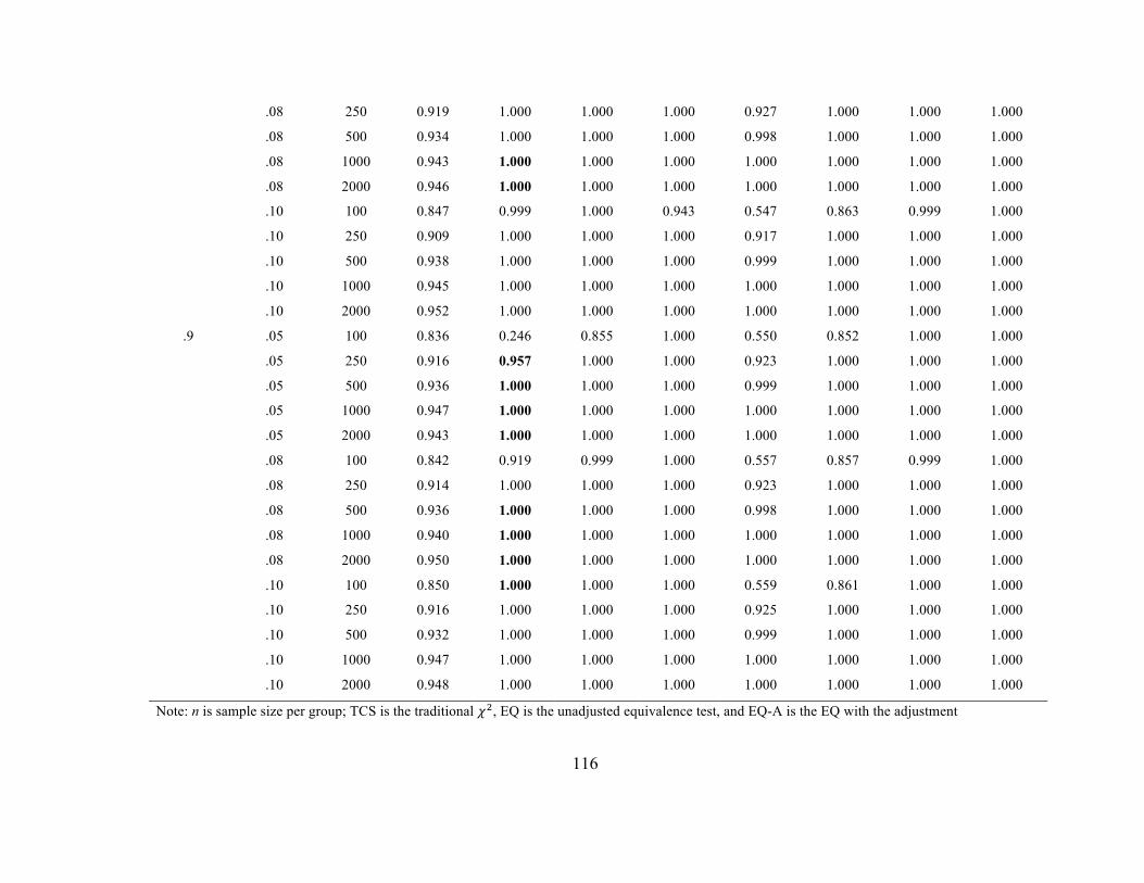
116
.08 250 0.919 1.000 1.000 1.000 0.927 1.000 1.000 1.000
.08 500 0.934 1.000 1.000 1.000 0.998 1.000 1.000 1.000
.08 1000 0.943 1.000 1.000 1.000 1.000 1.000 1.000 1.000
.08 2000 0.946 1.000 1.000 1.000 1.000 1.000 1.000 1.000
.10 100 0.847 0.999 1.000 0.943 0.547 0.863 0.999 1.000
.10 250 0.909 1.000 1.000 1.000 0.917 1.000 1.000 1.000
.10 500 0.938 1.000 1.000 1.000 0.999 1.000 1.000 1.000
.10 1000 0.945 1.000 1.000 1.000 1.000 1.000 1.000 1.000
.10 2000 0.952 1.000 1.000 1.000 1.000 1.000 1.000 1.000
.9 .05 100 0.836 0.246 0.855 1.000 0.550 0.852 1.000 1.000
.05 250 0.916 0.957 1.000 1.000 0.923 1.000 1.000 1.000
.05 500 0.936 1.000 1.000 1.000 0.999 1.000 1.000 1.000
.05 1000 0.947 1.000 1.000 1.000 1.000 1.000 1.000 1.000
.05 2000 0.943 1.000 1.000 1.000 1.000 1.000 1.000 1.000
.08 100 0.842 0.919 0.999 1.000 0.557 0.857 0.999 1.000
.08 250 0.914 1.000 1.000 1.000 0.923 1.000 1.000 1.000
.08 500 0.936 1.000 1.000 1.000 0.998 1.000 1.000 1.000
.08 1000 0.940 1.000 1.000 1.000 1.000 1.000 1.000 1.000
.08 2000 0.950 1.000 1.000 1.000 1.000 1.000 1.000 1.000
.10 100 0.850 1.000 1.000 1.000 0.559 0.861 1.000 1.000
.10 250 0.916 1.000 1.000 1.000 0.925 1.000 1.000 1.000
.10 500 0.932 1.000 1.000 1.000 0.999 1.000 1.000 1.000
.10 1000 0.947 1.000 1.000 1.000 1.000 1.000 1.000 1.000
.10 2000 0.948 1.000 1.000 1.000 1.000 1.000 1.000 1.000
Note: n is sample size per group; TCS is the traditional 𝜒!, EQ is the unadjusted equivalence test, and EQ-A is the EQ with the adjustment

117
Table 24 Power Rates for Group 2 Model Fit (8 indicator model) with No Model Misspecification Loadings RMSEA0 𝑛 TCS EQ EQ-A CFI95 MNCI95 RA05 RA08 RA10
.5 .05 100 0.849 0.246 0.865 0.576 0.549 0.862 1.000 1.000
.05 250 0.923 0.959 1.000 0.945 0.930 1.000 1.000 1.000
.05 500 0.931 1.000 1.000 0.999 0.999 1.000 1.000 1.000
.05 1000 0.937 1.000 1.000 1.000 1.000 1.000 1.000 1.000
.05 2000 0.948 1.000 1.000 1.000 1.000 1.000 1.000 1.000
.08 100 0.857 0.926 0.999 0.587 0.551 0.870 1.000 1.000
.08 250 0.923 1.000 1.000 0.945 0.931 1.000 1.000 1.000
.08 500 0.940 1.000 1.000 1.000 0.999 1.000 1.000 1.000
.08 1000 0.947 1.000 1.000 1.000 1.000 1.000 1.000 1.000
.08 2000 0.952 1.000 1.000 1.000 1.000 1.000 1.000 1.000
.10 100 0.842 0.999 1.000 0.568 0.546 0.857 1.000 1.000
.10 250 0.921 1.000 1.000 0.943 0.930 1.000 1.000 1.000
.10 500 0.942 1.000 1.000 0.999 0.999 1.000 1.000 1.000
.10 1000 0.944 1.000 1.000 1.000 1.000 1.000 1.000 1.000
.10 2000 0.944 1.000 1.000 1.000 1.000 1.000 1.000 1.000
.7 .05 100 0.840 0.240 0.855 0.937 0.541 0.853 0.999 1.000
.05 250 0.913 0.955 1.000 1.000 0.922 1.000 1.000 1.000
.05 500 0.932 1.000 1.000 1.000 0.998 1.000 1.000 1.000
.05 1000 0.944 1.000 1.000 1.000 1.000 1.000 1.000 1.000
.05 2000 0.949 1.000 1.000 1.000 1.000 1.000 1.000 1.000
.08 100 0.841 0.912 0.998 0.935 0.557 0.856 0.998 1.000

118
.08 250 0.918 1.000 1.000 1.000 0.929 1.000 1.000 1.000
.08 500 0.933 1.000 1.000 1.000 0.999 1.000 1.000 1.000
.08 1000 0.944 1.000 1.000 1.000 1.000 1.000 1.000 1.000
.08 2000 0.949 1.000 1.000 1.000 1.000 1.000 1.000 1.000
.10 100 0.839 0.999 1.000 0.939 0.543 0.853 0.999 1.000
.10 250 0.915 1.000 1.000 1.000 0.924 1.000 1.000 1.000
.10 500 0.936 1.000 1.000 1.000 0.999 1.000 1.000 1.000
.10 1000 0.944 1.000 1.000 1.000 1.000 1.000 1.000 1.000
.10 2000 0.952 1.000 1.000 1.000 1.000 1.000 1.000 1.000
.9 .05 100 0.839 0.250 0.857 1.000 0.548 0.854 0.999 1.000
.05 250 0.915 0.958 1.000 1.000 0.923 1.000 1.000 1.000
.05 500 0.939 1.000 1.000 1.000 0.999 1.000 1.000 1.000
.05 1000 0.945 1.000 1.000 1.000 1.000 1.000 1.000 1.000
.05 2000 0.946 1.000 1.000 1.000 1.000 1.000 1.000 1.000
.08 100 0.851 0.922 0.999 1.000 0.543 0.866 0.999 1.000
.08 250 0.923 1.000 1.000 1.000 0.931 1.000 1.000 1.000
.08 500 0.936 1.000 1.000 1.000 0.998 1.000 1.000 1.000
.08 1000 0.948 1.000 1.000 1.000 1.000 1.000 1.000 1.000
.08 2000 0.945 1.000 1.000 1.000 1.000 1.000 1.000 1.000
.10 100 0.846 0.999 1.000 1.000 0.541 0.861 0.999 1.000
.10 250 0.918 1.000 1.000 1.000 0.926 1.000 1.000 1.000
.10 500 0.939 1.000 1.000 1.000 0.999 1.000 1.000 1.000
.10 1000 0.943 1.000 1.000 1.000 1.000 1.000 1.000 1.000
.10 2000 0.944 1.000 1.000 1.000 1.000 1.000 1.000 1.000
Note: n is sample size per group; TCS is the traditional 𝜒!, EQ is the unadjusted equivalence test, and EQ-A is the EQ with the adjustment

119
Table 25 Power Rates for Configural Invariance (4 indicator model) with no Model Misspecification Loadings RMSEA0 𝑛 TCS EQ EQ-A CFI95 MNCI95 RA05 RA08 RA10
.5 .05 100 0.875 0.016 0.560 0.491 0.847 0.565 0.901 0.983
.05 250 0.891 0.164 0.914 0.822 0.998 0.910 0.999 1.000
.05 500 0.899 0.708 0.997 0.980 1.000 0.996 1.000 1.000
.05 1000 0.903 0.998 1.000 1.000 1.000 1.000 1.000 1.000
.05 2000 0.901 1.000 1.000 1.000 1.000 1.000 1.000 1.000
.08 100 0.866 0.147 0.903 0.487 0.838 0.564 0.895 0.983
.08 250 0.895 0.896 1.000 0.823 0.998 0.913 1.000 1.000
.08 500 0.892 1.000 1.000 0.980 1.000 0.996 1.000 1.000
.08 1000 0.904 1.000 1.000 1.000 1.000 1.000 1.000 1.000
.08 2000 0.901 1.000 1.000 1.000 1.000 1.000 1.000 1.000
.10 100 0.871 0.449 0.987 0.493 0.843 0.567 0.902 0.986
.10 250 0.888 0.997 1.000 0.816 0.999 0.904 1.000 1.000
.10 500 0.899 1.000 1.000 0.985 1.000 0.997 1.000 1.000
.10 1000 0.904 1.000 1.000 1.000 1.000 1.000 1.000 1.000
.10 2000 0.901 1.000 1.000 1.000 1.000 1.000 1.000 1.000
.7 .05 100 0.874 0.016 0.559 0.905 0.846 0.564 0.899 0.983
.05 250 0.884 0.163 0.911 1.000 0.998 0.905 0.999 1.000
.05 500 0.892 0.719 0.997 1.000 1.000 0.996 1.000 1.000
.05 1000 0.898 0.998 1.000 1.000 1.000 1.000 1.000 1.000
.05 2000 0.901 1.000 1.000 1.000 1.000 1.000 1.000 1.000
.08 100 0.861 0.139 0.897 0.893 0.833 0.555 0.889 0.980

120
.08 250 0.880 0.881 1.000 1.000 0.999 0.897 1.000 1.000
.08 500 0.892 1.000 1.000 1.000 1.000 0.997 1.000 1.000
.08 1000 0.900 1.000 1.000 1.000 1.000 1.000 1.000 1.000
.08 2000 0.894 1.000 1.000 1.000 1.000 1.000 1.000 1.000
.10 100 0.868 0.439 0.982 0.893 0.838 0.556 0.892 0.979
.10 250 0.890 0.998 1.000 1.000 0.999 0.911 1.000 1.000
.10 500 0.895 1.000 1.000 1.000 1.000 0.996 1.000 1.000
.10 1000 0.898 1.000 1.000 1.000 1.000 1.000 1.000 1.000
.10 2000 0.908 1.000 1.000 1.000 1.000 1.000 1.000 1.000
.9 .05 100 0.857 0.014 0.543 1.000 0.830 0.549 0.886 0.975
.05 250 0.882 0.148 0.906 1.000 0.998 0.901 0.999 1.000
.05 500 0.894 0.710 0.996 1.000 1.000 0.995 1.000 1.000
.05 1000 0.900 0.998 1.000 1.000 1.000 1.000 1.000 1.000
.05 2000 0.905 1.000 1.000 1.000 1.000 1.000 1.000 1.000
.08 100 0.856 0.136 0.894 1.000 0.824 0.533 0.887 0.977
.08 250 0.884 0.886 1.000 1.000 0.997 0.902 1.000 1.000
.08 500 0.893 1.000 1.000 1.000 1.000 0.998 1.000 1.000
.08 1000 0.896 1.000 1.000 1.000 1.000 1.000 1.000 1.000
.08 2000 0.895 1.000 1.000 1.000 1.000 1.000 1.000 1.000
.10 100 0.859 0.427 0.983 1.000 0.828 0.542 0.885 0.980
.10 250 0.884 0.997 1.000 1.000 0.998 0.901 1.000 1.000
.10 500 0.896 1.000 1.000 1.000 1.000 0.997 1.000 1.000
.10 1000 0.899 1.000 1.000 1.000 1.000 1.000 1.000 1.000
.10 2000 0.903 1.000 1.000 1.000 1.000 1.000 1.000 1.000
Note: n is sample size per group; TCS is the traditional 𝜒!, EQ is the unadjusted equivalence test, and EQ-A is the EQ with the adjustment
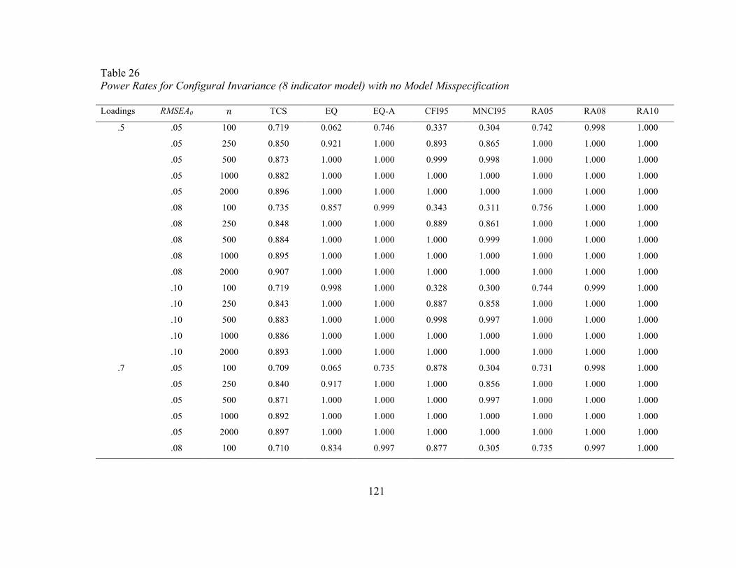
121
Table 26 Power Rates for Configural Invariance (8 indicator model) with no Model Misspecification Loadings RMSEA0 𝑛 TCS EQ EQ-A CFI95 MNCI95 RA05 RA08 RA10
.5 .05 100 0.719 0.062 0.746 0.337 0.304 0.742 0.998 1.000
.05 250 0.850 0.921 1.000 0.893 0.865 1.000 1.000 1.000
.05 500 0.873 1.000 1.000 0.999 0.998 1.000 1.000 1.000
.05 1000 0.882 1.000 1.000 1.000 1.000 1.000 1.000 1.000
.05 2000 0.896 1.000 1.000 1.000 1.000 1.000 1.000 1.000
.08 100 0.735 0.857 0.999 0.343 0.311 0.756 1.000 1.000
.08 250 0.848 1.000 1.000 0.889 0.861 1.000 1.000 1.000
.08 500 0.884 1.000 1.000 1.000 0.999 1.000 1.000 1.000
.08 1000 0.895 1.000 1.000 1.000 1.000 1.000 1.000 1.000
.08 2000 0.907 1.000 1.000 1.000 1.000 1.000 1.000 1.000
.10 100 0.719 0.998 1.000 0.328 0.300 0.744 0.999 1.000
.10 250 0.843 1.000 1.000 0.887 0.858 1.000 1.000 1.000
.10 500 0.883 1.000 1.000 0.998 0.997 1.000 1.000 1.000
.10 1000 0.886 1.000 1.000 1.000 1.000 1.000 1.000 1.000
.10 2000 0.893 1.000 1.000 1.000 1.000 1.000 1.000 1.000
.7 .05 100 0.709 0.065 0.735 0.878 0.304 0.731 0.998 1.000
.05 250 0.840 0.917 1.000 1.000 0.856 1.000 1.000 1.000
.05 500 0.871 1.000 1.000 1.000 0.997 1.000 1.000 1.000
.05 1000 0.892 1.000 1.000 1.000 1.000 1.000 1.000 1.000
.05 2000 0.897 1.000 1.000 1.000 1.000 1.000 1.000 1.000
.08 100 0.710 0.834 0.997 0.877 0.305 0.735 0.997 1.000

122
.08 250 0.842 1.000 1.000 1.000 0.859 1.000 1.000 1.000
.08 500 0.872 1.000 1.000 1.000 0.997 1.000 1.000 1.000
.08 1000 0.890 1.000 1.000 1.000 1.000 1.000 1.000 1.000
.08 2000 0.898 1.000 1.000 1.000 1.000 1.000 1.000 1.000
.10 100 0.712 0.998 1.000 0.885 0.296 0.736 0.999 1.000
.10 250 0.833 1.000 1.000 1.000 0.848 1.000 1.000 1.000
.10 500 0.877 1.000 1.000 1.000 0.998 1.000 1.000 1.000
.10 1000 0.892 1.000 1.000 1.000 1.000 1.000 1.000 1.000
.10 2000 0.907 1.000 1.000 1.000 1.000 1.000 1.000 1.000
.9 .05 100 0.702 0.064 0.731 1.000 0.305 0.727 0.999 1.000
.05 250 0.839 0.917 1.000 1.000 0.853 1.000 1.000 1.000
.05 500 0.879 1.000 1.000 1.000 0.998 1.000 1.000 1.000
.05 1000 0.894 1.000 1.000 1.000 1.000 1.000 1.000 1.000
.05 2000 0.894 1.000 1.000 1.000 1.000 1.000 1.000 1.000
.08 100 0.716 0.847 0.998 1.000 0.301 0.742 0.998 1.000
.08 250 0.845 1.000 1.000 1.000 0.859 1.000 1.000 1.000
.08 500 0.877 1.000 1.000 1.000 0.996 1.000 1.000 1.000
.08 1000 0.891 1.000 1.000 1.000 1.000 1.000 1.000 1.000
.08 2000 0.898 1.000 1.000 1.000 1.000 1.000 1.000 1.000
.10 100 0.721 0.999 1.000 1.000 0.303 0.744 0.999 1.000
.10 250 0.840 1.000 1.000 1.000 0.857 1.000 1.000 1.000
.10 500 0.877 1.000 1.000 1.000 0.998 1.000 1.000 1.000
.10 1000 0.894 1.000 1.000 1.000 1.000 1.000 1.000 1.000
.10 2000 0.894 1.000 1.000 1.000 1.000 1.000 1.000 1.000
Note: n is sample size per group; TCS is the traditional 𝜒!, EQ is the unadjusted equivalence test, and EQ-A is the EQ with the adjustment

123
Table 27 Power for Group 1 Model Fit (4 indicator model) with Small degree of Model Misspecification Loadings RMSEA0 𝑛 TCS EQ EQ-A CFI95 MNCI95 RA05 RA08 RA10
.5 .05 100 0.878 0.071 0.642 0.597 0.858 0.644 0.894 0.973
.05 250 0.791 0.170 0.828 0.714 0.987 0.820 0.994 1.000
.05 500 0.538 0.329 0.927 0.800 1.000 0.921 1.000 1.000
.05 1000 0.182 0.616 0.980 0.899 1.000 0.980 1.000 1.000
.05 2000 0.004 0.914 0.999 0.973 1.000 0.999 1.000 1.000
.08 100 0.883 0.267 0.906 0.576 0.862 0.628 0.900 0.978
.08 250 0.774 0.776 0.993 0.688 0.983 0.799 0.992 1.000
.08 500 0.536 0.989 1.000 0.783 1.000 0.908 1.000 1.000
.08 1000 0.176 1.000 1.000 0.902 1.000 0.985 1.000 1.000
.08 2000 0.005 1.000 1.000 0.963 1.000 1.000 1.000 1.000
.10 100 0.879 0.550 0.986 0.594 0.855 0.651 0.906 0.983
.10 250 0.774 0.983 1.000 0.698 0.991 0.798 0.997 1.000
.10 500 0.555 1.000 1.000 0.806 1.000 0.915 1.000 1.000
.10 1000 0.180 1.000 1.000 0.901 1.000 0.985 1.000 1.000
.10 2000 0.007 1.000 1.000 0.972 1.000 0.999 1.000 1.000
.7 .05 100 0.871 0.076 0.644 0.901 0.847 0.649 0.897 0.975
.05 250 0.773 0.167 0.809 0.996 0.991 0.801 0.996 1.000
.05 500 0.571 0.353 0.927 1.000 1.000 0.923 1.000 1.000
.05 1000 0.200 0.653 0.984 1.000 1.000 0.983 1.000 1.000
.05 2000 0.008 0.934 0.999 1.000 1.000 1.000 1.000 1.000
.08 100 0.875 0.265 0.906 0.900 0.853 0.630 0.898 0.975

124
.08 250 0.774 0.776 0.995 0.993 0.987 0.799 0.994 1.000
.08 500 0.572 0.990 1.000 1.000 1.000 0.917 1.000 1.000
.08 1000 0.193 1.000 1.000 1.000 1.000 0.986 1.000 1.000
.08 2000 0.010 1.000 1.000 1.000 1.000 0.999 1.000 1.000
.10 100 0.876 0.535 0.980 0.902 0.854 0.633 0.897 0.977
.10 250 0.786 0.988 1.000 0.999 0.991 0.816 0.997 1.000
.10 500 0.558 1.000 1.000 1.000 1.000 0.910 1.000 1.000
.10 1000 0.195 1.000 1.000 1.000 1.000 0.986 1.000 1.000
.10 2000 0.007 1.000 1.000 1.000 1.000 1.000 1.000 1.000
.9 .05 100 0.884 0.085 0.645 1.000 0.861 0.651 0.905 0.976
.05 250 0.775 0.160 0.800 1.000 0.985 0.795 0.995 1.000
.05 500 0.576 0.351 0.931 1.000 1.000 0.926 1.000 1.000
.05 1000 0.212 0.672 0.988 1.000 1.000 0.987 1.000 1.000
.05 2000 0.006 0.933 0.999 1.000 1.000 0.999 1.000 1.000
.08 100 0.886 0.271 0.914 1.000 0.865 0.647 0.910 0.976
.08 250 0.787 0.789 0.997 1.000 0.988 0.808 0.997 1.000
.08 500 0.563 0.989 1.000 1.000 1.000 0.914 1.000 1.000
.08 1000 0.206 1.000 1.000 1.000 1.000 0.990 1.000 1.000
.08 2000 0.009 1.000 1.000 1.000 1.000 1.000 1.000 1.000
.10 100 0.868 0.543 0.978 1.000 0.845 0.634 0.892 0.972
.10 250 0.783 0.983 1.000 1.000 0.987 0.807 0.996 1.000
.10 500 0.587 1.000 1.000 1.000 1.000 0.929 1.000 1.000
.10 1000 0.190 1.000 1.000 1.000 1.000 0.986 1.000 1.000
.10 2000 0.006 1.000 1.000 1.000 1.000 0.999 1.000 1.000
Note: n is sample size per group; TCS is the traditional 𝜒!, EQ is the unadjusted equivalence test, and EQ-A is the EQ with the adjustment
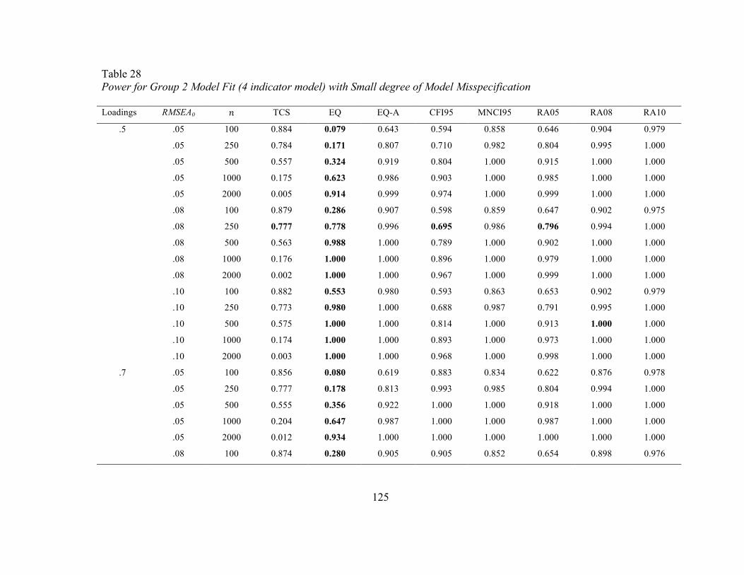
125
Table 28 Power for Group 2 Model Fit (4 indicator model) with Small degree of Model Misspecification Loadings RMSEA0 𝑛 TCS EQ EQ-A CFI95 MNCI95 RA05 RA08 RA10
.5 .05 100 0.884 0.079 0.643 0.594 0.858 0.646 0.904 0.979
.05 250 0.784 0.171 0.807 0.710 0.982 0.804 0.995 1.000
.05 500 0.557 0.324 0.919 0.804 1.000 0.915 1.000 1.000
.05 1000 0.175 0.623 0.986 0.903 1.000 0.985 1.000 1.000
.05 2000 0.005 0.914 0.999 0.974 1.000 0.999 1.000 1.000
.08 100 0.879 0.286 0.907 0.598 0.859 0.647 0.902 0.975
.08 250 0.777 0.778 0.996 0.695 0.986 0.796 0.994 1.000
.08 500 0.563 0.988 1.000 0.789 1.000 0.902 1.000 1.000
.08 1000 0.176 1.000 1.000 0.896 1.000 0.979 1.000 1.000
.08 2000 0.002 1.000 1.000 0.967 1.000 0.999 1.000 1.000
.10 100 0.882 0.553 0.980 0.593 0.863 0.653 0.902 0.979
.10 250 0.773 0.980 1.000 0.688 0.987 0.791 0.995 1.000
.10 500 0.575 1.000 1.000 0.814 1.000 0.913 1.000 1.000
.10 1000 0.174 1.000 1.000 0.893 1.000 0.973 1.000 1.000
.10 2000 0.003 1.000 1.000 0.968 1.000 0.998 1.000 1.000
.7 .05 100 0.856 0.080 0.619 0.883 0.834 0.622 0.876 0.978
.05 250 0.777 0.178 0.813 0.993 0.985 0.804 0.994 1.000
.05 500 0.555 0.356 0.922 1.000 1.000 0.918 1.000 1.000
.05 1000 0.204 0.647 0.987 1.000 1.000 0.987 1.000 1.000
.05 2000 0.012 0.934 1.000 1.000 1.000 1.000 1.000 1.000
.08 100 0.874 0.280 0.905 0.905 0.852 0.654 0.898 0.976
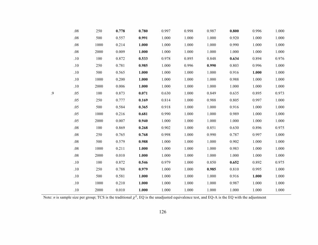
126
.08 250 0.778 0.780 0.997 0.998 0.987 0.800 0.996 1.000
.08 500 0.557 0.991 1.000 1.000 1.000 0.920 1.000 1.000
.08 1000 0.214 1.000 1.000 1.000 1.000 0.990 1.000 1.000
.08 2000 0.009 1.000 1.000 1.000 1.000 1.000 1.000 1.000
.10 100 0.872 0.533 0.978 0.895 0.848 0.634 0.894 0.976
.10 250 0.781 0.985 1.000 0.996 0.990 0.803 0.996 1.000
.10 500 0.565 1.000 1.000 1.000 1.000 0.916 1.000 1.000
.10 1000 0.200 1.000 1.000 1.000 1.000 0.988 1.000 1.000
.10 2000 0.006 1.000 1.000 1.000 1.000 1.000 1.000 1.000
.9 .05 100 0.873 0.071 0.630 1.000 0.849 0.635 0.895 0.973
.05 250 0.777 0.169 0.814 1.000 0.988 0.805 0.997 1.000
.05 500 0.584 0.365 0.918 1.000 1.000 0.916 1.000 1.000
.05 1000 0.216 0.681 0.990 1.000 1.000 0.989 1.000 1.000
.05 2000 0.007 0.940 1.000 1.000 1.000 1.000 1.000 1.000
.08 100 0.869 0.268 0.902 1.000 0.851 0.630 0.896 0.975
.08 250 0.765 0.768 0.998 1.000 0.990 0.787 0.997 1.000
.08 500 0.579 0.988 1.000 1.000 1.000 0.902 1.000 1.000
.08 1000 0.211 1.000 1.000 1.000 1.000 0.983 1.000 1.000
.08 2000 0.010 1.000 1.000 1.000 1.000 1.000 1.000 1.000
.10 100 0.872 0.546 0.979 1.000 0.850 0.652 0.892 0.975
.10 250 0.788 0.979 1.000 1.000 0.985 0.810 0.995 1.000
.10 500 0.581 1.000 1.000 1.000 1.000 0.916 1.000 1.000
.10 1000 0.210 1.000 1.000 1.000 1.000 0.987 1.000 1.000
.10 2000 0.010 1.000 1.000 1.000 1.000 1.000 1.000 1.000
Note: n is sample size per group; TCS is the traditional 𝜒!, EQ is the unadjusted equivalence test, and EQ-A is the EQ with the adjustment
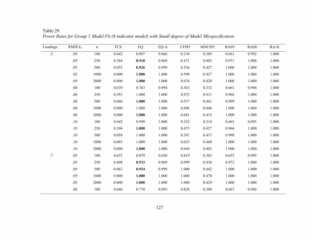
127
Table 29 Power Rates for Group 1 Model Fit (8 indicator model) with Small degree of Model Misspecification Loadings RMSEA0 𝑛 TCS EQ EQ-A CFI95 MNCI95 RA05 RA08 RA10
.5 .05 100 0.642 0.097 0.666 0.334 0.309 0.661 0.992 1.000
.05 250 0.384 0.510 0.969 0.471 0.403 0.971 1.000 1.000
.05 500 0.055 0.926 0.999 0.536 0.427 1.000 1.000 1.000
.05 1000 0.000 1.000 1.000 0.598 0.427 1.000 1.000 1.000
.05 2000 0.000 1.000 1.000 0.676 0.420 1.000 1.000 1.000
.08 100 0.639 0.763 0.994 0.363 0.332 0.661 0.996 1.000
.08 250 0.391 1.000 1.000 0.473 0.411 0.966 1.000 1.000
.08 500 0.066 1.000 1.000 0.537 0.441 0.999 1.000 1.000
.08 1000 0.000 1.000 1.000 0.606 0.446 1.000 1.000 1.000
.08 2000 0.000 1.000 1.000 0.681 0.415 1.000 1.000 1.000
.10 100 0.642 0.990 1.000 0.332 0.314 0.665 0.995 1.000
.10 250 0.396 1.000 1.000 0.473 0.427 0.966 1.000 1.000
.10 500 0.058 1.000 1.000 0.547 0.437 0.998 1.000 1.000
.10 1000 0.001 1.000 1.000 0.623 0.460 1.000 1.000 1.000
.10 2000 0.000 1.000 1.000 0.644 0.403 1.000 1.000 1.000
.7 .05 100 0.633 0.079 0.658 0.819 0.303 0.655 0.995 1.000
.05 250 0.408 0.533 0.969 0.999 0.436 0.972 1.000 1.000
.05 500 0.063 0.924 0.999 1.000 0.442 1.000 1.000 1.000
.05 1000 0.000 1.000 1.000 1.000 0.470 1.000 1.000 1.000
.05 2000 0.000 1.000 1.000 1.000 0.429 1.000 1.000 1.000
.08 100 0.646 0.770 0.992 0.828 0.309 0.667 0.994 1.000
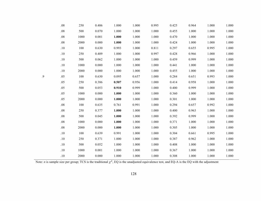
128
.08 250 0.406 1.000 1.000 0.995 0.425 0.964 1.000 1.000
.08 500 0.070 1.000 1.000 1.000 0.455 1.000 1.000 1.000
.08 1000 0.001 1.000 1.000 1.000 0.470 1.000 1.000 1.000
.08 2000 0.000 1.000 1.000 1.000 0.424 1.000 1.000 1.000
.10 100 0.630 0.993 1.000 0.811 0.297 0.655 0.995 1.000
.10 250 0.409 1.000 1.000 0.997 0.428 0.966 1.000 1.000
.10 500 0.062 1.000 1.000 1.000 0.459 0.999 1.000 1.000
.10 1000 0.000 1.000 1.000 1.000 0.441 1.000 1.000 1.000
.10 2000 0.000 1.000 1.000 1.000 0.455 1.000 1.000 1.000
.9 .05 100 0.630 0.095 0.657 1.000 0.284 0.651 0.993 1.000
.05 250 0.386 0.507 0.956 1.000 0.414 0.958 1.000 1.000
.05 500 0.053 0.910 0.999 1.000 0.400 0.999 1.000 1.000
.05 1000 0.000 1.000 1.000 1.000 0.360 1.000 1.000 1.000
.05 2000 0.000 1.000 1.000 1.000 0.301 1.000 1.000 1.000
.08 100 0.635 0.761 0.991 1.000 0.294 0.657 0.992 1.000
.08 250 0.377 1.000 1.000 1.000 0.400 0.963 1.000 1.000
.08 500 0.045 1.000 1.000 1.000 0.392 0.999 1.000 1.000
.08 1000 0.000 1.000 1.000 1.000 0.371 1.000 1.000 1.000
.08 2000 0.000 1.000 1.000 1.000 0.305 1.000 1.000 1.000
.10 100 0.639 0.991 1.000 1.000 0.304 0.661 0.995 1.000
.10 250 0.371 1.000 1.000 1.000 0.387 0.962 1.000 1.000
.10 500 0.052 1.000 1.000 1.000 0.408 1.000 1.000 1.000
.10 1000 0.001 1.000 1.000 1.000 0.367 1.000 1.000 1.000
.10 2000 0.000 1.000 1.000 1.000 0.308 1.000 1.000 1.000
Note: n is sample size per group; TCS is the traditional 𝜒!, EQ is the unadjusted equivalence test, and EQ-A is the EQ with the adjustment

129
Table 30 Power Rates for Group 2 Model Fit (8 indicator model) with Small degree of Model Misspecification Loadings RMSEA0 𝑛 TCS EQ EQ-A CFI95 MNCI95 RA05 RA08 RA10
.5 .05 100 0.650 0.111 0.680 0.328 0.304 0.678 0.992 1.000
.05 250 0.389 0.524 0.961 0.474 0.412 0.963 1.000 1.000
.05 500 0.058 0.939 1.000 0.554 0.445 1.000 1.000 1.000
.05 1000 0.000 1.000 1.000 0.611 0.428 1.000 1.000 1.000
.05 2000 0.000 1.000 1.000 0.658 0.397 1.000 1.000 1.000
.08 100 0.640 0.764 0.991 0.341 0.315 0.662 0.994 1.000
.08 250 0.406 1.000 1.000 0.490 0.425 0.967 1.000 1.000
.08 500 0.061 1.000 1.000 0.549 0.446 1.000 1.000 1.000
.08 1000 0.000 1.000 1.000 0.620 0.449 1.000 1.000 1.000
.08 2000 0.000 1.000 1.000 0.667 0.421 1.000 1.000 1.000
.10 100 0.651 0.994 1.000 0.328 0.306 0.678 0.997 1.000
.10 250 0.393 1.000 1.000 0.470 0.417 0.966 1.000 1.000
.10 500 0.062 1.000 1.000 0.565 0.458 1.000 1.000 1.000
.10 1000 0.000 1.000 1.000 0.611 0.429 1.000 1.000 1.000
.10 2000 0.000 1.000 1.000 0.692 0.442 1.000 1.000 1.000
.7 .05 100 0.636 0.087 0.661 0.814 0.291 0.656 0.993 1.000
.05 250 0.403 0.518 0.971 0.999 0.424 0.973 1.000 1.000
.05 500 0.063 0.927 0.999 1.000 0.447 0.999 1.000 1.000
.05 1000 0.000 1.000 1.000 1.000 0.472 1.000 1.000 1.000
.05 2000 0.000 1.000 1.000 1.000 0.452 1.000 1.000 1.000
.08 100 0.628 0.770 0.993 0.821 0.286 0.655 0.993 1.000

130
.08 250 0.411 1.000 1.000 0.998 0.429 0.967 1.000 1.000
.08 500 0.078 1.000 1.000 1.000 0.461 1.000 1.000 1.000
.08 1000 0.000 1.000 1.000 1.000 0.453 1.000 1.000 1.000
.08 2000 0.000 1.000 1.000 1.000 0.441 1.000 1.000 1.000
.10 100 0.663 0.991 1.000 0.839 0.332 0.686 0.994 1.000
.10 250 0.397 1.000 1.000 0.996 0.418 0.971 1.000 1.000
.10 500 0.063 1.000 1.000 1.000 0.451 1.000 1.000 1.000
.10 1000 0.000 1.000 1.000 1.000 0.463 1.000 1.000 1.000
.10 2000 0.000 1.000 1.000 1.000 0.433 1.000 1.000 1.000
.9 .05 100 0.641 0.099 0.673 1.000 0.298 0.668 0.993 1.000
.05 250 0.352 0.486 0.953 1.000 0.383 0.954 1.000 1.000
.05 500 0.046 0.912 1.000 1.000 0.384 1.000 1.000 1.000
.05 1000 0.000 0.999 1.000 1.000 0.369 1.000 1.000 1.000
.05 2000 0.000 1.000 1.000 1.000 0.314 1.000 1.000 1.000
.08 100 0.613 0.742 0.993 1.000 0.266 0.635 0.995 1.000
.08 250 0.365 1.000 1.000 1.000 0.387 0.960 1.000 1.000
.08 500 0.053 1.000 1.000 1.000 0.422 1.000 1.000 1.000
.08 1000 0.000 1.000 1.000 1.000 0.369 1.000 1.000 1.000
.08 2000 0.000 1.000 1.000 1.000 0.301 1.000 1.000 1.000
.10 100 0.625 0.990 1.000 1.000 0.288 0.644 0.993 1.000
.10 250 0.365 1.000 1.000 1.000 0.386 0.967 1.000 1.000
.10 500 0.054 1.000 1.000 1.000 0.404 0.998 1.000 1.000
.10 1000 0.000 1.000 1.000 1.000 0.387 1.000 1.000 1.000
.10 2000 0.000 1.000 1.000 1.000 0.306 1.000 1.000 1.000
Note: n is sample size per group; TCS is the traditional 𝜒!, EQ is the unadjusted equivalence test, and EQ-A is the EQ with the adjustment

131
Table 31 Power Rates for Configural Invariance (4 indicator model with small degree of model misspecification) Loadings RMSEA0 𝑛 TCS EQ EQ-A CFI95 MNCI95 RA05 RA08 RA10
.5 .05 100 0.780 0.004 0.412 0.353 0.740 0.416 0.812 0.952
.05 250 0.621 0.036 0.669 0.514 0.969 0.661 0.988 1.000
.05 500 0.300 0.099 0.850 0.642 1.000 0.842 1.000 1.000
.05 1000 0.034 0.379 0.967 0.812 1.000 0.966 1.000 1.000
.05 2000 0.000 0.836 0.998 0.947 1.000 0.998 1.000 1.000
.08 100 0.774 0.076 0.823 0.343 0.740 0.411 0.811 0.953
.08 250 0.610 0.614 0.989 0.483 0.970 0.643 0.986 1.000
.08 500 0.305 0.976 1.000 0.615 1.000 0.818 1.000 1.000
.08 1000 0.027 1.000 1.000 0.809 1.000 0.964 1.000 1.000
.08 2000 0.000 1.000 1.000 0.930 1.000 0.998 1.000 1.000
.10 100 0.773 0.302 0.967 0.350 0.737 0.424 0.816 0.962
.10 250 0.602 0.964 1.000 0.481 0.978 0.634 0.992 1.000
.10 500 0.311 1.000 1.000 0.653 0.999 0.835 1.000 1.000
.10 1000 0.033 1.000 1.000 0.802 1.000 0.957 1.000 1.000
.10 2000 0.000 1.000 1.000 0.940 1.000 0.997 1.000 1.000
.7 .05 100 0.748 0.008 0.400 0.799 0.710 0.406 0.788 0.953
.05 250 0.604 0.032 0.661 0.990 0.976 0.647 0.990 1.000
.05 500 0.315 0.127 0.857 1.000 1.000 0.850 1.000 1.000
.05 1000 0.038 0.428 0.972 1.000 1.000 0.971 1.000 1.000
.05 2000 0.000 0.871 0.999 1.000 1.000 1.000 1.000 1.000
.08 100 0.767 0.083 0.822 0.817 0.730 0.417 0.809 0.953

132
.08 250 0.602 0.606 0.993 0.992 0.974 0.635 0.990 1.000
.08 500 0.327 0.981 1.000 1.000 1.000 0.844 1.000 1.000
.08 1000 0.043 1.000 1.000 1.000 1.000 0.976 1.000 1.000
.08 2000 0.000 1.000 1.000 1.000 1.000 0.999 1.000 1.000
.10 100 0.764 0.287 0.958 0.807 0.722 0.404 0.804 0.953
.10 250 0.617 0.973 1.000 0.994 0.981 0.654 0.993 1.000
.10 500 0.306 1.000 1.000 1.000 1.000 0.833 1.000 1.000
.10 1000 0.035 1.000 1.000 1.000 1.000 0.974 1.000 1.000
.10 2000 0.000 1.000 1.000 1.000 1.000 1.000 1.000 1.000
.9 .05 100 0.772 0.010 0.411 1.000 0.732 0.416 0.810 0.950
.05 250 0.600 0.025 0.649 1.000 0.973 0.636 0.992 1.000
.05 500 0.341 0.131 0.853 1.000 1.000 0.847 1.000 1.000
.05 1000 0.044 0.457 0.978 1.000 1.000 0.976 1.000 1.000
.05 2000 0.000 0.877 0.999 1.000 1.000 0.999 1.000 1.000
.08 100 0.772 0.072 0.826 1.000 0.737 0.408 0.818 0.952
.08 250 0.601 0.605 0.995 1.000 0.977 0.634 0.994 1.000
.08 500 0.331 0.977 1.000 1.000 1.000 0.824 1.000 1.000
.08 1000 0.040 1.000 1.000 1.000 1.000 0.973 1.000 1.000
.08 2000 0.001 1.000 1.000 1.000 1.000 0.999 1.000 1.000
.10 100 0.757 0.299 0.957 1.000 0.720 0.410 0.796 0.948
.10 250 0.617 0.962 1.000 1.000 0.972 0.652 0.991 1.000
.10 500 0.337 1.000 1.000 1.000 1.000 0.850 1.000 1.000
.10 1000 0.038 1.000 1.000 1.000 1.000 0.973 1.000 1.000
.10 2000 0.000 1.000 1.000 1.000 1.000 0.999 1.000 1.000
Note: n is sample size per group; TCS is the traditional 𝜒!, EQ is the unadjusted equivalence test, and EQ-A is the EQ with the adjustment

133
Table 32 Power Rates for Configural Invariance (8 indicator model with small degree of model misspecification) Loadings RMSEA0 𝑛 TCS EQ EQ-A CFI95 MNCI95 RA05 RA08 RA10
.5 .05 100 0.417 0.009 0.454 0.106 0.090 0.449 0.984 1.000
.05 250 0.156 0.269 0.931 0.231 0.174 0.935 1.000 1.000
.05 500 0.006 0.870 0.999 0.286 0.178 1.000 1.000 1.000
.05 1000 0.000 1.000 1.000 0.363 0.187 1.000 1.000 1.000
.05 2000 0.000 1.000 1.000 0.446 0.180 1.000 1.000 1.000
.08 100 0.414 0.586 0.985 0.128 0.108 0.442 0.990 1.000
.08 250 0.162 1.000 1.000 0.237 0.181 0.935 1.000 1.000
.08 500 0.006 1.000 1.000 0.299 0.200 0.999 1.000 1.000
.08 1000 0.000 1.000 1.000 0.372 0.193 1.000 1.000 1.000
.08 2000 0.000 1.000 1.000 0.450 0.172 1.000 1.000 1.000
.10 100 0.413 0.984 1.000 0.101 0.092 0.449 0.992 1.000
.10 250 0.172 1.000 1.000 0.231 0.192 0.936 1.000 1.000
.10 500 0.004 1.000 1.000 0.311 0.196 0.998 1.000 1.000
.10 1000 0.000 1.000 1.000 0.390 0.195 1.000 1.000 1.000
.10 2000 0.000 1.000 1.000 0.446 0.179 1.000 1.000 1.000
.7 .05 100 0.396 0.008 0.429 0.667 0.088 0.423 0.987 1.000
.05 250 0.160 0.281 0.942 0.997 0.184 0.946 1.000 1.000
.05 500 0.004 0.856 0.998 1.000 0.194 0.999 1.000 1.000
.05 1000 0.000 1.000 1.000 1.000 0.222 1.000 1.000 1.000
.05 2000 0.000 1.000 1.000 1.000 0.190 1.000 1.000 1.000
.08 100 0.402 0.594 0.985 0.685 0.079 0.433 0.987 1.000

134
.08 250 0.167 1.000 1.000 0.993 0.183 0.932 1.000 1.000
.08 500 0.004 1.000 1.000 1.000 0.202 1.000 1.000 1.000
.08 1000 0.000 1.000 1.000 1.000 0.227 1.000 1.000 1.000
.08 2000 0.000 1.000 1.000 1.000 0.186 1.000 1.000 1.000
.10 100 0.418 0.984 1.000 0.682 0.092 0.449 0.989 1.000
.10 250 0.171 1.000 1.000 0.993 0.190 0.938 1.000 1.000
.10 500 0.007 1.000 1.000 1.000 0.202 0.999 1.000 1.000
.10 1000 0.000 1.000 1.000 1.000 0.214 1.000 1.000 1.000
.10 2000 0.000 1.000 1.000 1.000 0.200 1.000 1.000 1.000
.9 .05 100 0.414 0.013 0.448 1.000 0.089 0.443 0.986 1.000
.05 250 0.142 0.246 0.910 1.000 0.161 0.914 1.000 1.000
.05 500 0.002 0.830 0.999 1.000 0.152 0.999 1.000 1.000
.05 1000 0.000 0.999 1.000 1.000 0.127 1.000 1.000 1.000
.05 2000 0.000 1.000 1.000 1.000 0.086 1.000 1.000 1.000
.08 100 0.394 0.575 0.983 1.000 0.077 0.422 0.987 1.000
.08 250 0.133 1.000 1.000 1.000 0.152 0.925 1.000 1.000
.08 500 0.003 1.000 1.000 1.000 0.176 0.999 1.000 1.000
.08 1000 0.000 1.000 1.000 1.000 0.140 1.000 1.000 1.000
.08 2000 0.000 1.000 1.000 1.000 0.085 1.000 1.000 1.000
.10 100 0.395 0.981 1.000 1.000 0.081 0.424 0.988 1.000
.10 250 0.138 1.000 1.000 1.000 0.152 0.930 1.000 1.000
.10 500 0.004 1.000 1.000 1.000 0.167 0.998 1.000 1.000
.10 1000 0.000 1.000 1.000 1.000 0.139 1.000 1.000 1.000
.10 2000 0.000 1.000 1.000 1.000 0.088 1.000 1.000 1.000
Note: n is sample size per group; TCS is the traditional 𝜒!, EQ is the unadjusted equivalence test, and EQ-A is the EQ with the adjustment

135
Table 33 Power Rates for Metric Invariance (4 indicator identical group population models) Rel RMSEA0 𝑛 TCS EQ EQ-A ∆RMSEA ∆CFI ∆MNCI
.5 .05 100 0.808 0.001 0.360 0.582 0.456 0.750
.05 250 0.835 0.026 0.774 0.846 0.669 0.983
.05 500 0.856 0.276 0.964 0.935 0.864 1.000
.05 1000 0.858 0.813 0.998 0.981 0.972 1.000
.05 2000 0.856 0.997 1.000 0.998 0.999 1.000
.08 100 0.802 0.023 0.745 0.709 0.456 0.743
.08 250 0.839 0.463 0.984 0.853 0.662 0.983
.08 500 0.842 0.915 1.000 0.928 0.855 1.000
.08 1000 0.858 1.000 1.000 0.981 0.972 1.000
.08 2000 0.859 1.000 1.000 0.998 0.998 1.000
.10 100 0.804 0.116 0.905 0.730 0.468 0.754
.10 250 0.838 0.793 0.998 0.861 0.675 0.984
.10 500 0.856 0.995 1.000 0.936 0.878 1.000
.10 1000 0.856 1.000 1.000 0.977 0.969 1.000
.10 2000 0.855 1.000 1.000 0.997 0.999 1.000
.7 .05 100 0.819 0.001 0.386 0.582 0.728 0.761
.05 250 0.838 0.028 0.782 0.861 0.958 0.986
.05 500 0.847 0.285 0.963 0.935 0.995 1.000
.05 1000 0.848 0.810 0.999 0.979 1.000 1.000
.05 2000 0.856 0.994 1.000 0.997 1.000 1.000
.08 100 0.816 0.024 0.769 0.726 0.732 0.764
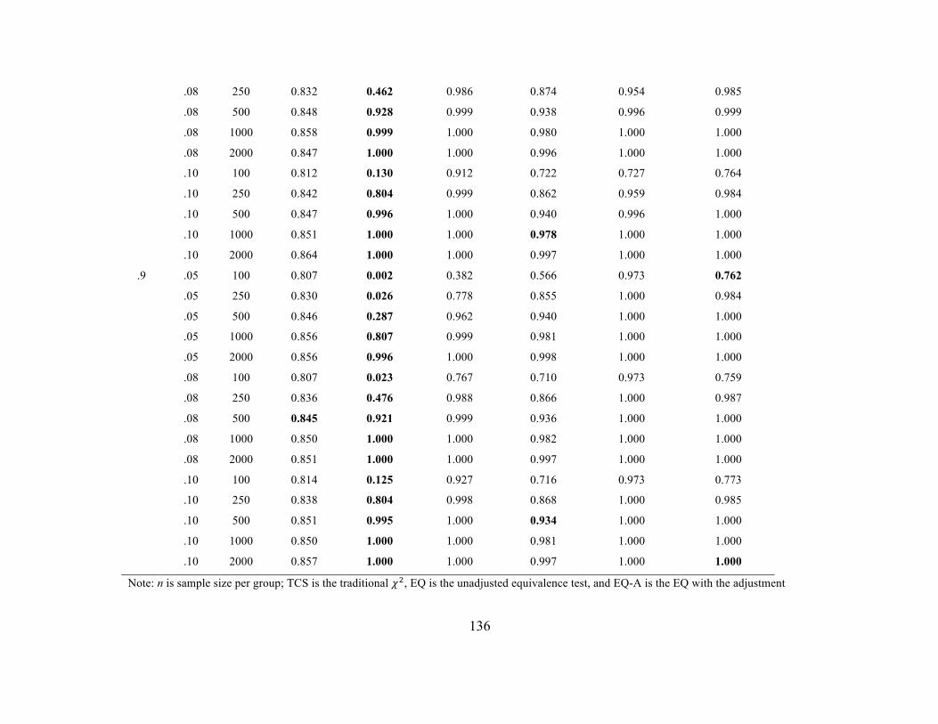
136
.08 250 0.832 0.462 0.986 0.874 0.954 0.985
.08 500 0.848 0.928 0.999 0.938 0.996 0.999
.08 1000 0.858 0.999 1.000 0.980 1.000 1.000
.08 2000 0.847 1.000 1.000 0.996 1.000 1.000
.10 100 0.812 0.130 0.912 0.722 0.727 0.764
.10 250 0.842 0.804 0.999 0.862 0.959 0.984
.10 500 0.847 0.996 1.000 0.940 0.996 1.000
.10 1000 0.851 1.000 1.000 0.978 1.000 1.000
.10 2000 0.864 1.000 1.000 0.997 1.000 1.000
.9 .05 100 0.807 0.002 0.382 0.566 0.973 0.762
.05 250 0.830 0.026 0.778 0.855 1.000 0.984
.05 500 0.846 0.287 0.962 0.940 1.000 1.000
.05 1000 0.856 0.807 0.999 0.981 1.000 1.000
.05 2000 0.856 0.996 1.000 0.998 1.000 1.000
.08 100 0.807 0.023 0.767 0.710 0.973 0.759
.08 250 0.836 0.476 0.988 0.866 1.000 0.987
.08 500 0.845 0.921 0.999 0.936 1.000 1.000
.08 1000 0.850 1.000 1.000 0.982 1.000 1.000
.08 2000 0.851 1.000 1.000 0.997 1.000 1.000
.10 100 0.814 0.125 0.927 0.716 0.973 0.773
.10 250 0.838 0.804 0.998 0.868 1.000 0.985
.10 500 0.851 0.995 1.000 0.934 1.000 1.000
.10 1000 0.850 1.000 1.000 0.981 1.000 1.000
.10 2000 0.857 1.000 1.000 0.997 1.000 1.000
Note: n is sample size per group; TCS is the traditional 𝜒!, EQ is the unadjusted equivalence test, and EQ-A is the EQ with the adjustment

137
Table 34 Power Rates for Metric Invariance (8 indicator identical group population models) Rel RMSEA0 𝑛 TCS EQ EQ-A ∆RMSEA ∆CFI ∆MNCI
.5 .05 100 0.674 0.007 0.541 0.871 0.327 0.304
.05 250 0.798 0.285 0.926 0.979 0.819 0.922
.05 500 0.827 0.733 0.994 0.997 0.977 0.998
.05 1000 0.836 0.992 1.000 1.000 0.999 1.000
.05 2000 0.848 1.000 1.000 1.000 1.000 1.000
.08 100 0.683 0.247 0.918 0.932 0.337 0.328
.08 250 0.797 0.858 0.999 0.979 0.807 0.919
.08 500 0.839 0.999 1.000 0.997 0.972 0.997
.08 1000 0.850 1.000 1.000 1.000 0.999 1.000
.08 2000 0.862 1.000 1.000 1.000 1.000 1.000
.10 100 0.675 0.529 0.987 0.933 0.327 0.312
.10 250 0.795 0.987 1.000 0.977 0.805 0.923
.10 500 0.835 1.000 1.000 0.998 0.975 0.999
.10 1000 0.848 1.000 1.000 1.000 0.999 1.000
.10 2000 0.842 1.000 1.000 1.000 1.000 1.000
.7 .05 100 0.664 0.009 0.540 0.866 0.830 0.303
.05 250 0.802 0.305 0.943 0.984 0.997 0.931
.05 500 0.828 0.732 0.996 0.998 1.000 0.999
.05 1000 0.850 0.993 1.000 1.000 1.000 1.000
.05 2000 0.856 1.000 1.000 1.000 1.000 1.000
.08 100 0.666 0.273 0.932 0.942 0.839 0.313

138
.08 250 0.794 0.870 0.999 0.980 0.995 0.927
.08 500 0.830 0.999 1.000 0.998 1.000 0.998
.08 1000 0.847 1.000 1.000 1.000 1.000 1.000
.08 2000 0.852 1.000 1.000 1.000 1.000 1.000
.10 100 0.670 0.561 0.986 0.943 0.832 0.308
.10 250 0.785 0.990 1.000 0.980 0.995 0.921
.10 500 0.832 1.000 1.000 0.998 1.000 0.997
.10 1000 0.841 1.000 1.000 1.000 1.000 1.000
.10 2000 0.860 1.000 1.000 1.000 1.000 1.000
.9 .05 100 0.657 0.007 0.546 0.874 0.999 0.311
.05 250 0.792 0.300 0.931 0.979 1.000 0.929
.05 500 0.834 0.734 0.995 0.998 1.000 0.997
.05 1000 0.850 0.991 1.000 1.000 1.000 1.000
.05 2000 0.852 1.000 1.000 1.000 1.000 1.000
.08 100 0.671 0.282 0.931 0.939 0.998 0.319
.08 250 0.798 0.869 1.000 0.978 1.000 0.928
.08 500 0.834 0.998 1.000 0.996 1.000 0.996
.08 1000 0.842 1.000 1.000 1.000 1.000 1.000
.08 2000 0.853 1.000 1.000 1.000 1.000 1.000
.10 100 0.685 0.567 0.985 0.944 0.998 0.327
.10 250 0.798 0.991 1.000 0.982 1.000 0.929
.10 500 0.835 1.000 1.000 0.998 1.000 0.998
.10 1000 0.845 1.000 1.000 1.000 1.000 1.000
.10 2000 0.849 1.000 1.000 1.000 1.000 1.000
Note: n is sample size per group; TCS is the traditional 𝜒!, EQ is the unadjusted equivalence test, and EQ-A is the EQ with the adjustment

139
Table 35 Power Rates for Metric Invariance (4 indicator population models with small group difference in single loading) Rel RMSEA0 𝑛 TCS EQ EQ-A ∆RMSEA ∆CFI ∆MNCI
.5 .05 100 0.807 0.001 0.353 0.595 0.466 0.744
.05 250 0.783 0.018 0.694 0.813 0.607 0.954
.05 500 0.715 0.126 0.831 0.830 0.709 0.990
.05 1000 0.552 0.355 0.930 0.844 0.751 1.000
.05 2000 0.280 0.639 0.990 0.810 0.764 1.000
.08 100 0.786 0.020 0.710 0.697 0.468 0.709
.08 250 0.786 0.344 0.961 0.818 0.600 0.957
.08 500 0.731 0.758 0.996 0.854 0.738 0.997
.08 1000 0.552 0.969 1.000 0.836 0.740 1.000
.08 2000 0.280 1.000 1.000 0.816 0.744 1.000
.10 100 0.791 0.103 0.872 0.714 0.447 0.704
.10 250 0.782 0.664 0.992 0.813 0.596 0.953
.10 500 0.717 0.965 1.000 0.844 0.714 0.995
.10 1000 0.555 1.000 1.000 0.838 0.740 1.000
.10 2000 0.258 1.000 1.000 0.797 0.756 1.000
.7 .05 100 0.792 0.000 0.343 0.577 0.710 0.738
.05 250 0.780 0.014 0.671 0.784 0.905 0.952
.05 500 0.718 0.126 0.838 0.844 0.964 0.992
.05 1000 0.503 0.317 0.911 0.819 0.992 1.000
.05 2000 0.208 0.544 0.981 0.747 1.000 1.000
.08 100 0.805 0.021 0.728 0.707 0.702 0.724

140
.08 250 0.764 0.338 0.961 0.817 0.898 0.958
.08 500 0.705 0.722 0.997 0.834 0.962 0.997
.08 1000 0.501 0.973 1.000 0.821 0.994 1.000
.08 2000 0.192 1.000 1.000 0.743 1.000 1.000
.10 100 0.789 0.105 0.892 0.723 0.700 0.721
.10 250 0.775 0.669 0.993 0.816 0.903 0.948
.10 500 0.709 0.957 0.999 0.835 0.962 0.996
.10 1000 0.524 1.000 1.000 0.812 0.994 1.000
.10 2000 0.199 1.000 1.000 0.769 1.000 1.000
.9 .05 100 0.789 0.002 0.342 0.567 0.958 0.741
.05 250 0.766 0.020 0.664 0.816 1.000 0.951
.05 500 0.690 0.124 0.822 0.837 1.000 0.992
.05 1000 0.495 0.304 0.913 0.799 1.000 1.000
.05 2000 0.195 0.541 0.977 0.729 1.000 1.000
.08 100 0.791 0.021 0.717 0.700 0.965 0.717
.08 250 0.775 0.335 0.958 0.821 0.998 0.955
.08 500 0.695 0.723 0.995 0.836 1.000 0.996
.08 1000 0.492 0.965 1.000 0.799 1.000 1.000
.08 2000 0.206 1.000 1.000 0.754 1.000 1.000
.10 100 0.793 0.096 0.894 0.688 0.956 0.725
.10 250 0.778 0.669 0.992 0.826 1.000 0.959
.10 500 0.682 0.947 1.000 0.836 1.000 0.995
.10 1000 0.518 1.000 1.000 0.793 1.000 1.000
.10 2000 0.199 1.000 1.000 0.748 1.000 1.000
Note: n is sample size per group; TCS is the traditional 𝜒!, EQ is the unadjusted equivalence test, and EQ-A is the EQ with the adjustment

141
Table 36 Power Rates for Metric Invariance (8 indicator population models with small group difference in single loading) Rel RMSEA0 𝑛 TCS EQ EQ-A ∆RMSEA ∆CFI ∆MNCI
.5 .05 100 0.631 0.004 0.455 0.842 0.314 0.286
.05 250 0.676 0.114 0.773 0.951 0.682 0.799
.05 500 0.528 0.252 0.887 0.950 0.760 0.925
.05 1000 0.213 0.457 0.950 0.953 0.777 0.980
.05 2000 0.015 0.768 0.991 0.970 0.836 0.999
.08 100 0.654 0.193 0.871 0.925 0.306 0.306
.08 250 0.668 0.633 0.990 0.942 0.680 0.783
.08 500 0.496 0.952 1.000 0.950 0.736 0.905
.08 1000 0.202 1.000 1.000 0.966 0.795 0.989
.08 2000 0.013 1.000 1.000 0.969 0.846 1.000
.10 100 0.640 0.397 0.955 0.922 0.290 0.294
.10 250 0.689 0.934 1.000 0.956 0.681 0.800
.10 500 0.527 0.999 1.000 0.955 0.759 0.919
.10 1000 0.216 1.000 1.000 0.953 0.792 0.983
.10 2000 0.011 1.000 1.000 0.971 0.850 0.998
.7 .05 100 0.638 0.008 0.489 0.859 0.797 0.301
.05 250 0.698 0.132 0.786 0.951 0.963 0.821
.05 500 0.576 0.304 0.896 0.957 0.998 0.929
.05 1000 0.282 0.565 0.971 0.975 1.000 0.991
.05 2000 0.028 0.849 0.997 0.975 1.000 1.000
.08 100 0.630 0.196 0.882 0.924 0.793 0.294

142
.08 250 0.685 0.677 0.991 0.951 0.967 0.811
.08 500 0.590 0.963 0.999 0.964 0.998 0.938
.08 1000 0.300 1.000 1.000 0.975 1.000 0.992
.08 2000 0.029 1.000 1.000 0.981 1.000 1.000
.10 100 0.665 0.470 0.979 0.933 0.802 0.311
.10 250 0.697 0.944 1.000 0.955 0.973 0.828
.10 500 0.585 1.000 1.000 0.960 0.999 0.940
.10 1000 0.286 1.000 1.000 0.969 1.000 0.989
.10 2000 0.030 1.000 1.000 0.978 1.000 1.000
.9 .05 100 0.638 0.006 0.467 0.863 0.995 0.278
.05 250 0.671 0.123 0.767 0.951 1.000 0.805
.05 500 0.559 0.263 0.880 0.959 1.000 0.936
.05 1000 0.243 0.508 0.964 0.966 1.000 0.984
.05 2000 0.019 0.794 0.999 0.974 1.000 1.000
.08 100 0.637 0.186 0.886 0.925 0.992 0.290
.08 250 0.698 0.682 0.992 0.954 1.000 0.814
.08 500 0.547 0.951 0.999 0.950 1.000 0.925
.08 1000 0.232 1.000 1.000 0.966 1.000 0.988
.08 2000 0.019 1.000 1.000 0.969 1.000 0.999
.10 100 0.647 0.462 0.973 0.937 0.995 0.300
.10 250 0.684 0.933 0.999 0.954 1.000 0.805
.10 500 0.539 1.000 1.000 0.961 1.000 0.928
.10 1000 0.231 1.000 1.000 0.967 1.000 0.986
.10 2000 0.019 1.000 1.000 0.966 1.000 1.000
Note: n is sample size per group; TCS is the traditional 𝜒!, EQ is the unadjusted equivalence test, and EQ-A is the EQ with the adjustment

143
Table 37 Power Rates for Scalar Invariance (4 indicator identical group population models) Rel RMSEA0 𝑛 TCS EQ EQ-A ∆RMSEA ∆CFI ∆MNCI
.5 .05 100 0.769 0.000 0.255 0.479 0.387 0.597
.05 250 0.791 0.005 0.666 0.762 0.537 0.972
.05 500 0.812 0.111 0.931 0.893 0.770 1.000
.05 1000 0.815 0.660 0.997 0.967 0.948 1.000
.05 2000 0.816 0.994 1.000 0.997 0.997 1.000
.08 100 0.757 0.005 0.647 0.586 0.386 0.588
.08 250 0.796 0.244 0.972 0.772 0.532 0.969
.08 500 0.796 0.841 1.000 0.884 0.754 1.000
.08 1000 0.816 0.999 1.000 0.970 0.951 1.000
.08 2000 0.816 1.000 1.000 0.997 0.996 1.000
.10 100 0.764 0.035 0.851 0.596 0.393 0.598
.10 250 0.791 0.638 0.997 0.778 0.538 0.968
.10 500 0.812 0.990 1.000 0.889 0.782 1.000
.10 1000 0.814 1.000 1.000 0.962 0.942 1.000
.10 2000 0.812 1.000 1.000 0.996 0.997 1.000
.7 .05 100 0.775 0.000 0.273 0.477 0.584 0.599
.05 250 0.798 0.004 0.676 0.783 0.922 0.973
.05 500 0.800 0.113 0.928 0.882 0.991 1.000
.05 1000 0.808 0.658 0.998 0.968 1.000 1.000
.05 2000 0.810 0.990 1.000 0.995 1.000 1.000
.08 100 0.771 0.004 0.666 0.588 0.588 0.599
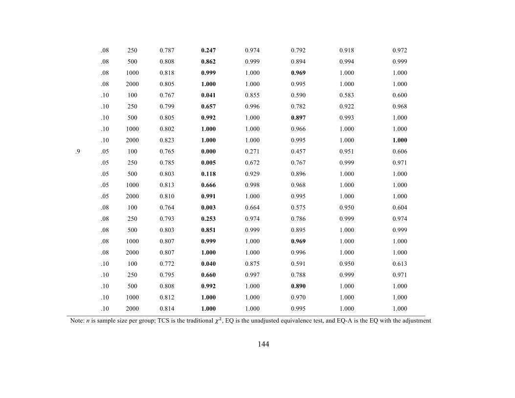
144
.08 250 0.787 0.247 0.974 0.792 0.918 0.972
.08 500 0.808 0.862 0.999 0.894 0.994 0.999
.08 1000 0.818 0.999 1.000 0.969 1.000 1.000
.08 2000 0.805 1.000 1.000 0.995 1.000 1.000
.10 100 0.767 0.041 0.855 0.590 0.583 0.600
.10 250 0.799 0.657 0.996 0.782 0.922 0.968
.10 500 0.805 0.992 1.000 0.897 0.993 1.000
.10 1000 0.802 1.000 1.000 0.966 1.000 1.000
.10 2000 0.823 1.000 1.000 0.995 1.000 1.000
.9 .05 100 0.765 0.000 0.271 0.457 0.951 0.606
.05 250 0.785 0.005 0.672 0.767 0.999 0.971
.05 500 0.803 0.118 0.929 0.896 1.000 1.000
.05 1000 0.813 0.666 0.998 0.968 1.000 1.000
.05 2000 0.810 0.991 1.000 0.995 1.000 1.000
.08 100 0.764 0.003 0.664 0.575 0.950 0.604
.08 250 0.793 0.253 0.974 0.786 0.999 0.974
.08 500 0.803 0.851 0.999 0.895 1.000 0.999
.08 1000 0.807 0.999 1.000 0.969 1.000 1.000
.08 2000 0.807 1.000 1.000 0.996 1.000 1.000
.10 100 0.772 0.040 0.875 0.591 0.950 0.613
.10 250 0.795 0.660 0.997 0.788 0.999 0.971
.10 500 0.808 0.992 1.000 0.890 1.000 1.000
.10 1000 0.812 1.000 1.000 0.970 1.000 1.000
.10 2000 0.814 1.000 1.000 0.995 1.000 1.000
Note: n is sample size per group; TCS is the traditional 𝜒!, EQ is the unadjusted equivalence test, and EQ-A is the EQ with the adjustment

145
Table 38 Power Rates for Scalar Invariance (8 indicator identical group population models) Rel RMSEA0 𝑛 TCS EQ EQ-A ∆RMSEA ∆CFI ∆MNCI
.5 .05 100 0.629 0.001 0.398 0.830 0.237 0.170
.05 250 0.758 0.095 0.871 0.962 0.689 0.877
.05 500 0.784 0.534 0.990 0.995 0.954 0.996
.05 1000 0.794 0.982 1.000 1.000 0.998 1.000
.05 2000 0.808 1.000 1.000 1.000 1.000 1.000
.08 100 0.649 0.086 0.866 0.892 0.240 0.191
.08 250 0.756 0.741 0.999 0.966 0.690 0.871
.08 500 0.801 0.998 1.000 0.994 0.949 0.996
.08 1000 0.813 1.000 1.000 1.000 0.999 1.000
.08 2000 0.823 1.000 1.000 1.000 1.000 1.000
.10 100 0.637 0.309 0.973 0.889 0.233 0.171
.10 250 0.749 0.976 1.000 0.962 0.684 0.868
.10 500 0.791 1.000 1.000 0.996 0.954 0.996
.10 1000 0.808 1.000 1.000 1.000 0.998 1.000
.10 2000 0.803 1.000 1.000 1.000 1.000 1.000
.7 .05 100 0.626 0.001 0.408 0.823 0.716 0.171
.05 250 0.762 0.100 0.886 0.968 0.994 0.886
.05 500 0.786 0.536 0.991 0.997 1.000 0.996
.05 1000 0.806 0.983 1.000 1.000 1.000 1.000
.05 2000 0.810 1.000 1.000 1.000 1.000 1.000
.08 100 0.628 0.087 0.872 0.892 0.731 0.176

146
.08 250 0.754 0.757 0.999 0.963 0.992 0.879
.08 500 0.791 0.998 1.000 0.996 1.000 0.995
.08 1000 0.803 1.000 1.000 1.000 1.000 1.000
.08 2000 0.810 1.000 1.000 1.000 1.000 1.000
.10 100 0.633 0.315 0.971 0.901 0.715 0.179
.10 250 0.739 0.981 1.000 0.967 0.990 0.873
.10 500 0.791 1.000 1.000 0.997 1.000 0.994
.10 1000 0.801 1.000 1.000 1.000 1.000 1.000
.10 2000 0.818 1.000 1.000 1.000 1.000 1.000
.9 .05 100 0.620 0.001 0.410 0.830 0.996 0.170
.05 250 0.755 0.098 0.878 0.966 1.000 0.887
.05 500 0.792 0.535 0.989 0.996 1.000 0.995
.05 1000 0.808 0.980 1.000 1.000 1.000 1.000
.05 2000 0.809 1.000 1.000 1.000 1.000 1.000
.08 100 0.638 0.093 0.880 0.897 0.995 0.182
.08 250 0.759 0.751 0.999 0.964 1.000 0.880
.08 500 0.796 0.997 1.000 0.994 1.000 0.993
.08 1000 0.800 1.000 1.000 1.000 1.000 1.000
.08 2000 0.808 1.000 1.000 1.000 1.000 1.000
.10 100 0.643 0.332 0.966 0.895 0.995 0.180
.10 250 0.758 0.982 1.000 0.967 1.000 0.885
.10 500 0.795 1.000 1.000 0.997 1.000 0.996
.10 1000 0.799 1.000 1.000 1.000 1.000 1.000
.10 2000 0.805 1.000 1.000 1.000 1.000 1.000
Note: n is sample size per group; TCS is the traditional 𝜒!, EQ is the unadjusted equivalence test, and EQ-A is the EQ with the adjustment
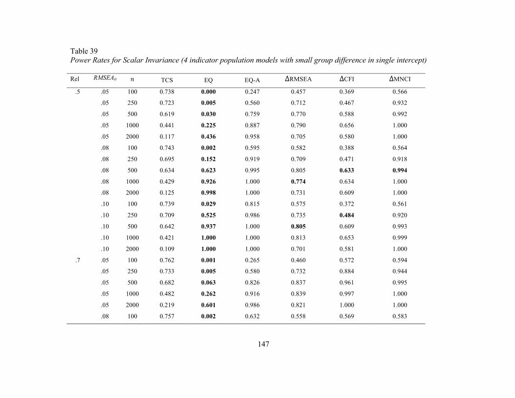
147
Table 39 Power Rates for Scalar Invariance (4 indicator population models with small group difference in single intercept) Rel RMSEA0 𝑛 TCS EQ EQ-A ∆RMSEA ∆CFI ∆MNCI
.5 .05 100 0.738 0.000 0.247 0.457 0.369 0.566
.05 250 0.723 0.005 0.560 0.712 0.467 0.932
.05 500 0.619 0.030 0.759 0.770 0.588 0.992
.05 1000 0.441 0.225 0.887 0.790 0.656 1.000
.05 2000 0.117 0.436 0.958 0.705 0.580 1.000
.08 100 0.743 0.002 0.595 0.582 0.388 0.564
.08 250 0.695 0.152 0.919 0.709 0.471 0.918
.08 500 0.634 0.623 0.995 0.805 0.633 0.994
.08 1000 0.429 0.926 1.000 0.774 0.634 1.000
.08 2000 0.125 0.998 1.000 0.731 0.609 1.000
.10 100 0.739 0.029 0.815 0.575 0.372 0.561
.10 250 0.709 0.525 0.986 0.735 0.484 0.920
.10 500 0.642 0.937 1.000 0.805 0.609 0.993
.10 1000 0.421 1.000 1.000 0.813 0.653 0.999
.10 2000 0.109 1.000 1.000 0.701 0.581 1.000
.7 .05 100 0.762 0.001 0.265 0.460 0.572 0.594
.05 250 0.733 0.005 0.580 0.732 0.884 0.944
.05 500 0.682 0.063 0.826 0.837 0.961 0.995
.05 1000 0.482 0.262 0.916 0.839 0.997 1.000
.05 2000 0.219 0.601 0.986 0.821 1.000 1.000
.08 100 0.757 0.002 0.632 0.558 0.569 0.583
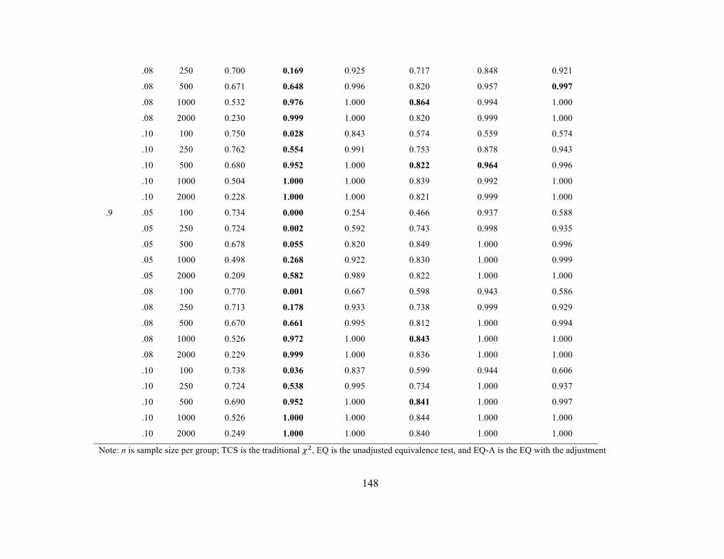
148
.08 250 0.700 0.169 0.925 0.717 0.848 0.921
.08 500 0.671 0.648 0.996 0.820 0.957 0.997
.08 1000 0.532 0.976 1.000 0.864 0.994 1.000
.08 2000 0.230 0.999 1.000 0.820 0.999 1.000
.10 100 0.750 0.028 0.843 0.574 0.559 0.574
.10 250 0.762 0.554 0.991 0.753 0.878 0.943
.10 500 0.680 0.952 1.000 0.822 0.964 0.996
.10 1000 0.504 1.000 1.000 0.839 0.992 1.000
.10 2000 0.228 1.000 1.000 0.821 0.999 1.000
.9 .05 100 0.734 0.000 0.254 0.466 0.937 0.588
.05 250 0.724 0.002 0.592 0.743 0.998 0.935
.05 500 0.678 0.055 0.820 0.849 1.000 0.996
.05 1000 0.498 0.268 0.922 0.830 1.000 0.999
.05 2000 0.209 0.582 0.989 0.822 1.000 1.000
.08 100 0.770 0.001 0.667 0.598 0.943 0.586
.08 250 0.713 0.178 0.933 0.738 0.999 0.929
.08 500 0.670 0.661 0.995 0.812 1.000 0.994
.08 1000 0.526 0.972 1.000 0.843 1.000 1.000
.08 2000 0.229 0.999 1.000 0.836 1.000 1.000
.10 100 0.738 0.036 0.837 0.599 0.944 0.606
.10 250 0.724 0.538 0.995 0.734 1.000 0.937
.10 500 0.690 0.952 1.000 0.841 1.000 0.997
.10 1000 0.526 1.000 1.000 0.844 1.000 1.000
.10 2000 0.249 1.000 1.000 0.840 1.000 1.000
Note: n is sample size per group; TCS is the traditional 𝜒!, EQ is the unadjusted equivalence test, and EQ-A is the EQ with the adjustment

149
Table 40 Power Rates for Scalar Invariance (8 indicator population models with small group difference in single intercept) Rel RMSEA0 𝑛 TCS EQ EQ-A ∆RMSEA ∆CFI ∆MNCI
.5 .05 100 0.600 0.001 0.361 0.839 0.241 0.177
.05 250 0.656 0.043 0.725 0.947 0.586 0.785
.05 500 0.533 0.197 0.897 0.967 0.776 0.938
.05 1000 0.282 0.570 0.976 0.972 0.850 0.994
.05 2000 0.026 0.855 1.000 0.989 0.909 0.999
.08 100 0.608 0.061 0.809 0.892 0.225 0.158
.08 250 0.638 0.550 0.994 0.931 0.595 0.758
.08 500 0.556 0.971 1.000 0.969 0.787 0.944
.08 1000 0.270 1.000 1.000 0.979 0.849 0.987
.08 2000 0.032 1.000 1.000 0.987 0.908 1.000
.10 100 0.644 0.250 0.966 0.894 0.251 0.185
.10 250 0.655 0.942 1.000 0.946 0.616 0.776
.10 500 0.521 1.000 1.000 0.959 0.762 0.930
.10 1000 0.265 1.000 1.000 0.982 0.862 0.986
.10 2000 0.035 1.000 1.000 0.990 0.911 1.000
.7 .05 100 0.594 0.001 0.347 0.835 0.687 0.176
.05 250 0.699 0.046 0.769 0.942 0.974 0.807
.05 500 0.562 0.237 0.906 0.967 0.998 0.935
.05 1000 0.282 0.555 0.970 0.979 1.000 0.990
.05 2000 0.025 0.859 0.999 0.988 1.000 0.999
.08 100 0.607 0.052 0.809 0.878 0.662 0.156

150
.08 250 0.654 0.587 0.992 0.932 0.963 0.759
.08 500 0.538 0.973 1.000 0.967 0.998 0.946
.08 1000 0.280 1.000 1.000 0.981 1.000 0.995
.08 2000 0.031 1.000 1.000 0.990 1.000 1.000
.10 100 0.615 0.295 0.966 0.894 0.711 0.182
.10 250 0.661 0.940 1.000 0.938 0.970 0.783
.10 500 0.542 1.000 1.000 0.975 0.997 0.934
.10 1000 0.268 1.000 1.000 0.979 1.000 0.992
.10 2000 0.042 1.000 1.000 0.986 1.000 1.000
.9 .05 100 0.609 0.000 0.356 0.841 0.994 0.171
.05 250 0.708 0.047 0.788 0.940 1.000 0.804
.05 500 0.571 0.275 0.929 0.973 1.000 0.955
.05 1000 0.333 0.643 0.980 0.986 1.000 0.991
.05 2000 0.054 0.923 0.998 0.997 1.000 1.000
.08 100 0.617 0.087 0.851 0.889 0.995 0.161
.08 250 0.659 0.609 0.992 0.947 1.000 0.773
.08 500 0.587 0.975 0.999 0.976 1.000 0.954
.08 1000 0.331 1.000 1.000 0.989 1.000 0.993
.08 2000 0.051 1.000 1.000 0.994 1.000 0.999
.10 100 0.600 0.251 0.961 0.907 0.995 0.151
.10 250 0.649 0.951 1.000 0.951 1.000 0.781
.10 500 0.560 1.000 1.000 0.974 1.000 0.953
.10 1000 0.312 1.000 1.000 0.988 1.000 0.995
.10 2000 0.050 1.000 1.000 0.995 1.000 1.000
Note: n is sample size per group; TCS is the traditional 𝜒!, EQ is the unadjusted equivalence test, and EQ-A is the EQ with the adjustment

151
Table 41 Power Rates for Strict Invariance (4 indicator identical group population models) Rel RMSEA0 𝑛 TCS EQ EQ-A ∆RMSEA ∆CFI ∆MNCI
.5 .05 100 0.718 0.000 0.180 0.403 0.342 0.404
.05 250 0.752 0.002 0.593 0.686 0.458 0.952
.05 500 0.772 0.055 0.914 0.853 0.675 0.999
.05 1000 0.775 0.597 0.997 0.953 0.912 1.000
.05 2000 0.777 0.994 1.000 0.996 0.995 1.000
.08 100 0.715 0.001 0.568 0.485 0.344 0.409
.08 250 0.757 0.160 0.966 0.694 0.451 0.953
.08 500 0.759 0.820 1.000 0.842 0.667 0.999
.08 1000 0.772 0.999 1.000 0.954 0.914 1.000
.08 2000 0.776 1.000 1.000 0.996 0.993 1.000
.10 100 0.720 0.015 0.817 0.494 0.352 0.418
.10 250 0.751 0.580 0.996 0.701 0.462 0.947
.10 500 0.771 0.990 1.000 0.847 0.684 1.000
.10 1000 0.770 1.000 1.000 0.944 0.906 1.000
.10 2000 0.771 1.000 1.000 0.994 0.994 1.000
.7 .05 100 0.733 0.000 0.191 0.395 0.484 0.416
.05 250 0.756 0.001 0.601 0.712 0.874 0.952
.05 500 0.758 0.055 0.910 0.840 0.986 0.999
.05 1000 0.768 0.598 0.998 0.957 1.000 1.000
.05 2000 0.764 0.990 1.000 0.994 1.000 1.000
.08 100 0.730 0.001 0.589 0.489 0.487 0.418

152
.08 250 0.743 0.162 0.968 0.715 0.869 0.952
.08 500 0.769 0.840 0.999 0.845 0.988 0.999
.08 1000 0.778 0.999 1.000 0.955 1.000 1.000
.08 2000 0.761 1.000 1.000 0.994 1.000 1.000
.10 100 0.719 0.013 0.814 0.490 0.480 0.414
.10 250 0.759 0.597 0.996 0.708 0.873 0.947
.10 500 0.768 0.992 1.000 0.853 0.987 0.999
.10 1000 0.764 1.000 1.000 0.953 1.000 1.000
.10 2000 0.781 1.000 1.000 0.994 1.000 1.000
.9 .05 100 0.715 0.000 0.190 0.384 0.913 0.416
.05 250 0.744 0.001 0.594 0.692 0.999 0.950
.05 500 0.759 0.062 0.909 0.857 1.000 0.999
.05 1000 0.769 0.603 0.998 0.955 1.000 1.000
.05 2000 0.772 0.991 1.000 0.994 1.000 1.000
.08 100 0.721 0.000 0.593 0.481 0.916 0.424
.08 250 0.753 0.161 0.970 0.715 0.999 0.956
.08 500 0.762 0.827 0.999 0.848 1.000 0.998
.08 1000 0.764 0.999 1.000 0.954 1.000 1.000
.08 2000 0.759 1.000 1.000 0.995 1.000 1.000
.10 100 0.728 0.013 0.837 0.489 0.916 0.438
.10 250 0.754 0.598 0.996 0.715 0.998 0.950
.10 500 0.763 0.991 1.000 0.843 1.000 0.999
.10 1000 0.768 1.000 1.000 0.957 1.000 1.000
.10 2000 0.776 1.000 1.000 0.994 1.000 1.000
Note: n is sample size per group; TCS is the traditional 𝜒!, EQ is the unadjusted equivalence test, and EQ-A is the EQ with the adjustment

153
Table 42 Power Rates for Strict Invariance (8 indicator identical group population models) Rel RMSEA0 𝑛 TCS EQ EQ-A ∆RMSEA ∆CFI ∆MNCI
.5 .05 100 0.590 0.000 0.291 0.791 0.192 0.085
.05 250 0.720 0.036 0.826 0.947 0.591 0.817
.05 500 0.746 0.416 0.986 0.993 0.928 0.992
.05 1000 0.757 0.978 1.000 1.000 0.997 1.000
.05 2000 0.767 1.000 1.000 1.000 1.000 1.000
.08 100 0.610 0.029 0.817 0.848 0.192 0.101
.08 250 0.713 0.670 0.999 0.953 0.582 0.812
.08 500 0.759 0.998 1.000 0.991 0.922 0.992
.08 1000 0.770 1.000 1.000 1.000 0.998 1.000
.08 2000 0.778 1.000 1.000 1.000 1.000 1.000
.10 100 0.597 0.185 0.959 0.852 0.192 0.092
.10 250 0.704 0.973 1.000 0.946 0.574 0.804
.10 500 0.750 1.000 1.000 0.995 0.929 0.993
.10 1000 0.767 1.000 1.000 1.000 0.997 1.000
.10 2000 0.764 1.000 1.000 1.000 1.000 1.000
.7 .05 100 0.587 0.000 0.294 0.782 0.603 0.083
.05 250 0.722 0.038 0.840 0.951 0.988 0.829
.05 500 0.743 0.421 0.989 0.995 1.000 0.995
.05 1000 0.772 0.980 1.000 1.000 1.000 1.000
.05 2000 0.773 1.000 1.000 1.000 1.000 1.000
.08 100 0.588 0.030 0.819 0.850 0.618 0.088

154
.08 250 0.711 0.686 0.998 0.948 0.986 0.818
.08 500 0.749 0.998 1.000 0.995 1.000 0.993
.08 1000 0.768 1.000 1.000 1.000 1.000 1.000
.08 2000 0.768 1.000 1.000 1.000 1.000 1.000
.10 100 0.589 0.187 0.954 0.855 0.606 0.094
.10 250 0.701 0.977 1.000 0.952 0.986 0.817
.10 500 0.751 1.000 1.000 0.993 1.000 0.992
.10 1000 0.759 1.000 1.000 1.000 1.000 1.000
.10 2000 0.777 1.000 1.000 1.000 1.000 1.000
.9 .05 100 0.585 0.000 0.307 0.795 0.992 0.086
.05 250 0.709 0.035 0.822 0.949 1.000 0.819
.05 500 0.757 0.424 0.989 0.994 1.000 0.994
.05 1000 0.766 0.976 1.000 1.000 1.000 1.000
.05 2000 0.768 1.000 1.000 1.000 1.000 1.000
.08 100 0.601 0.029 0.830 0.860 0.992 0.094
.08 250 0.719 0.685 0.999 0.947 1.000 0.825
.08 500 0.750 0.997 1.000 0.992 1.000 0.991
.08 1000 0.754 1.000 1.000 1.000 1.000 1.000
.08 2000 0.769 1.000 1.000 1.000 1.000 1.000
.10 100 0.600 0.195 0.957 0.850 0.993 0.095
.10 250 0.721 0.976 1.000 0.950 1.000 0.826
.10 500 0.752 1.000 1.000 0.995 1.000 0.994
.10 1000 0.758 1.000 1.000 1.000 1.000 1.000
.10 2000 0.764 1.000 1.000 1.000 1.000 1.000
Note: n is sample size per group; TCS is the traditional 𝜒!, EQ is the unadjusted equivalence test, and EQ-A is the EQ with the adjustment
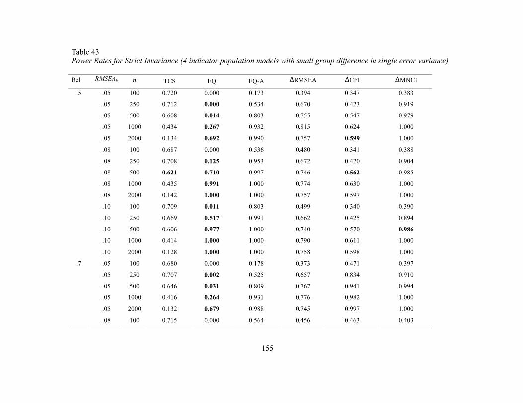
155
Table 43 Power Rates for Strict Invariance (4 indicator population models with small group difference in single error variance) Rel RMSEA0 𝑛 TCS EQ EQ-A ∆RMSEA ∆CFI ∆MNCI
.5 .05 100 0.720 0.000 0.173 0.394 0.347 0.383
.05 250 0.712 0.000 0.534 0.670 0.423 0.919
.05 500 0.608 0.014 0.803 0.755 0.547 0.979
.05 1000 0.434 0.267 0.932 0.815 0.624 1.000
.05 2000 0.134 0.692 0.990 0.757 0.599 1.000
.08 100 0.687 0.000 0.536 0.480 0.341 0.388
.08 250 0.708 0.125 0.953 0.672 0.420 0.904
.08 500 0.621 0.710 0.997 0.746 0.562 0.985
.08 1000 0.435 0.991 1.000 0.774 0.630 1.000
.08 2000 0.142 1.000 1.000 0.757 0.597 1.000
.10 100 0.709 0.011 0.803 0.499 0.340 0.390
.10 250 0.669 0.517 0.991 0.662 0.425 0.894
.10 500 0.606 0.977 1.000 0.740 0.570 0.986
.10 1000 0.414 1.000 1.000 0.790 0.611 1.000
.10 2000 0.128 1.000 1.000 0.758 0.598 1.000
.7 .05 100 0.680 0.000 0.178 0.373 0.471 0.397
.05 250 0.707 0.002 0.525 0.657 0.834 0.910
.05 500 0.646 0.031 0.809 0.767 0.941 0.994
.05 1000 0.416 0.264 0.931 0.776 0.982 1.000
.05 2000 0.132 0.679 0.988 0.745 0.997 1.000
.08 100 0.715 0.000 0.564 0.456 0.463 0.403

156
.08 250 0.703 0.117 0.946 0.669 0.831 0.911
.08 500 0.573 0.661 0.994 0.718 0.925 0.984
.08 1000 0.407 0.988 1.000 0.779 0.988 1.000
.08 2000 0.111 1.000 1.000 0.749 1.000 1.000
.10 100 0.695 0.012 0.796 0.497 0.461 0.403
.10 250 0.702 0.519 0.997 0.687 0.825 0.908
.10 500 0.603 0.965 1.000 0.738 0.928 0.979
.10 1000 0.449 1.000 1.000 0.790 0.986 0.999
.10 2000 0.116 1.000 1.000 0.719 0.998 1.000
.9 .05 100 0.696 0.000 0.151 0.390 0.899 0.414
.05 250 0.708 0.000 0.548 0.686 0.993 0.921
.05 500 0.624 0.023 0.811 0.750 1.000 0.985
.05 1000 0.453 0.301 0.950 0.805 1.000 1.000
.05 2000 0.140 0.691 0.996 0.764 1.000 1.000
.08 100 0.715 0.000 0.589 0.479 0.912 0.423
.08 250 0.706 0.117 0.938 0.696 0.999 0.903
.08 500 0.629 0.716 0.999 0.776 1.000 0.988
.08 1000 0.428 0.992 1.000 0.815 1.000 1.000
.08 2000 0.125 1.000 1.000 0.762 1.000 1.000
.10 100 0.709 0.014 0.811 0.475 0.912 0.397
.10 250 0.682 0.500 0.987 0.677 0.998 0.897
.10 500 0.600 0.972 1.000 0.764 1.000 0.989
.10 1000 0.424 1.000 1.000 0.775 1.000 1.000
.10 2000 0.131 1.000 1.000 0.775 1.000 1.000
Note: n is sample size per group; TCS is the traditional 𝜒!, EQ is the unadjusted equivalence test, and EQ-A is the EQ with the adjustment

157
Table 44 Power Rates for Strict Invariance (8 indicator population models with small group difference in single error variance) Rel RMSEA0 𝑛 TCS EQ EQ-A ∆RMSEA ∆CFI ∆MNCI
.5 .05 100 0.590 0.000 0.265 0.763 0.199 0.087
.05 250 0.628 0.012 0.713 0.923 0.529 0.702
.05 500 0.497 0.176 0.908 0.956 0.736 0.899
.05 1000 0.191 0.559 0.966 0.970 0.796 0.972
.05 2000 0.014 0.906 1.000 0.985 0.848 1.000
.08 100 0.558 0.025 0.742 0.847 0.206 0.076
.08 250 0.600 0.529 0.996 0.931 0.509 0.695
.08 500 0.500 0.985 1.000 0.957 0.755 0.917
.08 1000 0.198 1.000 1.000 0.969 0.799 0.975
.08 2000 0.017 1.000 1.000 0.990 0.857 0.998
.10 100 0.549 0.158 0.937 0.846 0.193 0.082
.10 250 0.591 0.949 1.000 0.935 0.514 0.683
.10 500 0.516 0.998 1.000 0.950 0.728 0.905
.10 1000 0.210 1.000 1.000 0.978 0.803 0.983
.10 2000 0.008 1.000 1.000 0.983 0.844 0.999
.7 .05 100 0.549 0.000 0.239 0.777 0.580 0.070
.05 250 0.603 0.014 0.691 0.912 0.947 0.694
.05 500 0.457 0.143 0.885 0.959 0.995 0.891
.05 1000 0.186 0.565 0.968 0.971 1.000 0.974
.05 2000 0.003 0.846 1.000 0.976 1.000 1.000
.08 100 0.585 0.037 0.784 0.853 0.612 0.080
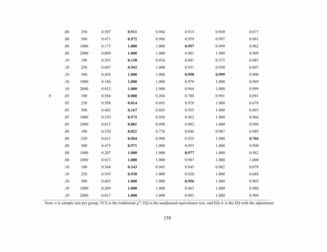
158
.08 250 0.587 0.511 0.986 0.915 0.949 0.677
.08 500 0.471 0.972 0.996 0.959 0.997 0.891
.08 1000 0.173 1.000 1.000 0.957 0.999 0.962
.08 2000 0.009 1.000 1.000 0.981 1.000 0.998
.10 100 0.543 0.138 0.934 0.841 0.572 0.083
.10 250 0.607 0.942 1.000 0.931 0.950 0.697
.10 500 0.456 1.000 1.000 0.958 0.999 0.900
.10 1000 0.186 1.000 1.000 0.970 1.000 0.969
.10 2000 0.012 1.000 1.000 0.984 1.000 0.999
.9 .05 100 0.584 0.000 0.284 0.788 0.991 0.091
.05 250 0.588 0.014 0.693 0.928 1.000 0.678
.05 500 0.482 0.167 0.885 0.955 1.000 0.893
.05 1000 0.193 0.572 0.958 0.963 1.000 0.966
.05 2000 0.013 0.881 0.998 0.982 1.000 0.998
.08 100 0.550 0.021 0.776 0.846 0.987 0.089
.08 250 0.621 0.564 0.990 0.925 1.000 0.704
.08 500 0.475 0.971 1.000 0.953 1.000 0.900
.08 1000 0.207 1.000 1.000 0.977 1.000 0.982
.08 2000 0.013 1.000 1.000 0.987 1.000 1.000
.10 100 0.564 0.143 0.945 0.845 0.982 0.078
.10 250 0.593 0.930 1.000 0.920 1.000 0.688
.10 500 0.493 1.000 1.000 0.956 1.000 0.905
.10 1000 0.209 1.000 1.000 0.963 1.000 0.980
.10 2000 0.017 1.000 1.000 0.983 1.000 0.998
Note: n is sample size per group; TCS is the traditional 𝜒!, EQ is the unadjusted equivalence test, and EQ-A is the EQ with the adjustment
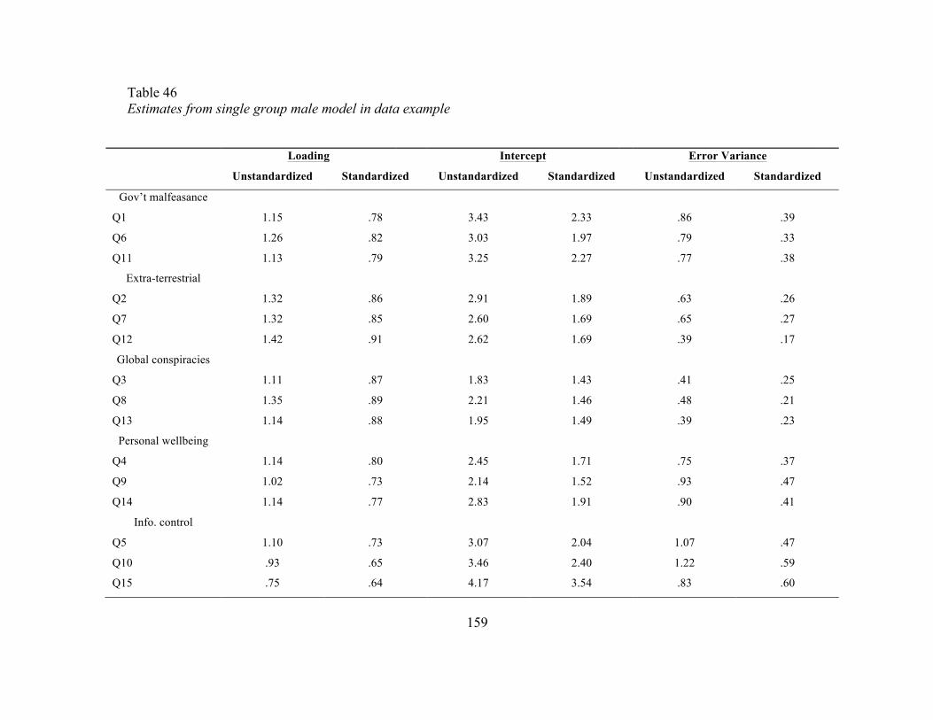
159
Table 46 Estimates from single group male model in data example
Loading Intercept Error Variance
Unstandardized Standardized Unstandardized Standardized Unstandardized Standardized
Gov’t malfeasance
Q1 1.15 .78 3.43 2.33 .86 .39
Q6 1.26 .82 3.03 1.97 .79 .33
Q11 1.13 .79 3.25 2.27 .77 .38
Extra-terrestrial
Q2 1.32 .86 2.91 1.89 .63 .26
Q7 1.32 .85 2.60 1.69 .65 .27
Q12 1.42 .91 2.62 1.69 .39 .17
Global conspiracies
Q3 1.11 .87 1.83 1.43 .41 .25
Q8 1.35 .89 2.21 1.46 .48 .21
Q13 1.14 .88 1.95 1.49 .39 .23
Personal wellbeing
Q4 1.14 .80 2.45 1.71 .75 .37
Q9 1.02 .73 2.14 1.52 .93 .47
Q14 1.14 .77 2.83 1.91 .90 .41
Info. control
Q5 1.10 .73 3.07 2.04 1.07 .47
Q10 .93 .65 3.46 2.40 1.22 .59
Q15 .75 .64 4.17 3.54 .83 .60
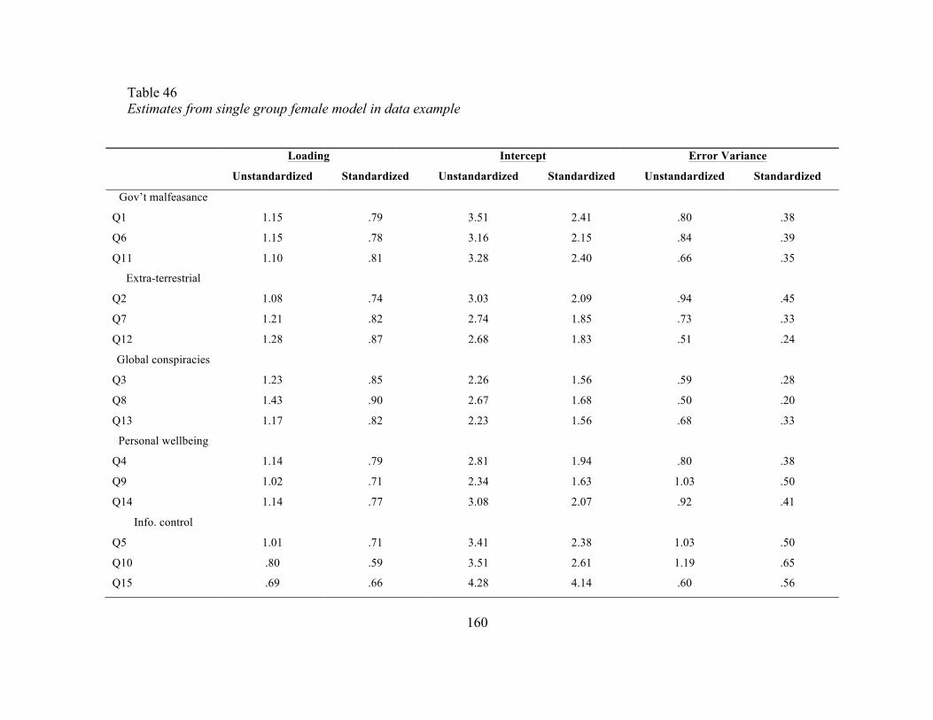
160
Table 46 Estimates from single group female model in data example
Loading Intercept Error Variance
Unstandardized Standardized Unstandardized Standardized Unstandardized Standardized
Gov’t malfeasance
Q1 1.15 .79 3.51 2.41 .80 .38
Q6 1.15 .78 3.16 2.15 .84 .39
Q11 1.10 .81 3.28 2.40 .66 .35
Extra-terrestrial
Q2 1.08 .74 3.03 2.09 .94 .45
Q7 1.21 .82 2.74 1.85 .73 .33
Q12 1.28 .87 2.68 1.83 .51 .24
Global conspiracies
Q3 1.23 .85 2.26 1.56 .59 .28
Q8 1.43 .90 2.67 1.68 .50 .20
Q13 1.17 .82 2.23 1.56 .68 .33
Personal wellbeing
Q4 1.14 .79 2.81 1.94 .80 .38
Q9 1.02 .71 2.34 1.63 1.03 .50
Q14 1.14 .77 3.08 2.07 .92 .41
Info. control
Q5 1.01 .71 3.41 2.38 1.03 .50
Q10 .80 .59 3.51 2.61 1.19 .65
Q15 .69 .66 4.28 4.14 .60 .56

161
Figure1. Path diagrams for each of the measurement models used in simulation. The top figure represents the four-indicator per factor model and the bottom half of the figure represents the eight-indicator per factor model. The population model loadings are either .5, .7 or .9 with corresponding error variances of .75, .51, and .19. All observed variables means were set at 1 and the latent means were set at 0 with variance of 1. In both models, the correlation between factors was .5.
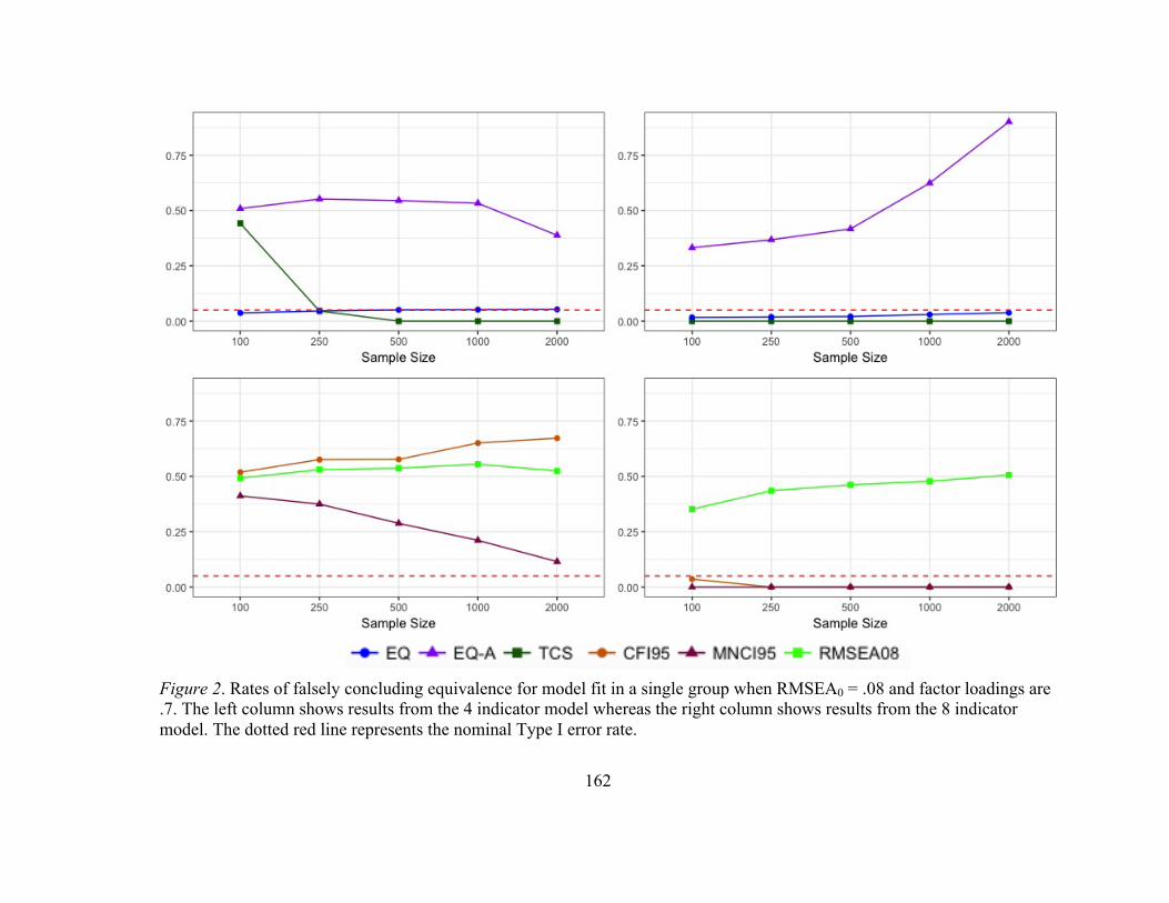
162
Figure 2. Rates of falsely concluding equivalence for model fit in a single group when RMSEA0 = .08 and factor loadings are .7. The left column shows results from the 4 indicator model whereas the right column shows results from the 8 indicator model. The dotted red line represents the nominal Type I error rate.

163
Figure 3. Rates of falsely concluding equivalence for metric invariance in the 4 indicator model when RMSEA0 = .08. The left column represents factor loadings of .5 (low) whereas the right column includes factor loadings at .9 (high). The dotted red line represents the nominal Type I error rate. Sample size is per group.
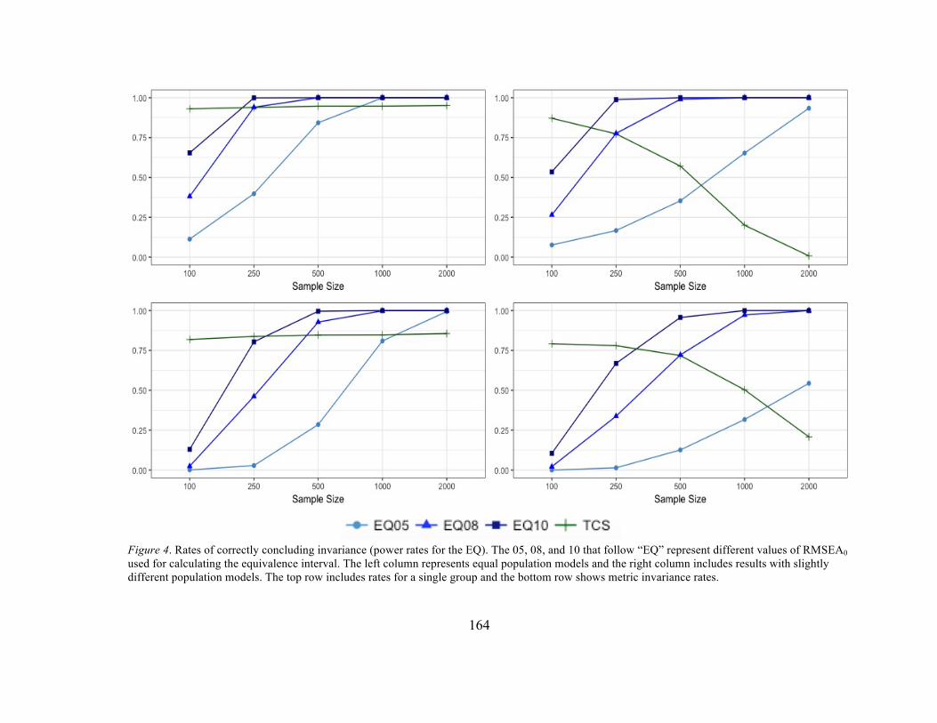
164
Figure 4. Rates of correctly concluding invariance (power rates for the EQ). The 05, 08, and 10 that follow “EQ” represent different values of RMSEA0 used for calculating the equivalence interval. The left column represents equal population models and the right column includes results with slightly different population models. The top row includes rates for a single group and the bottom row shows metric invariance rates.
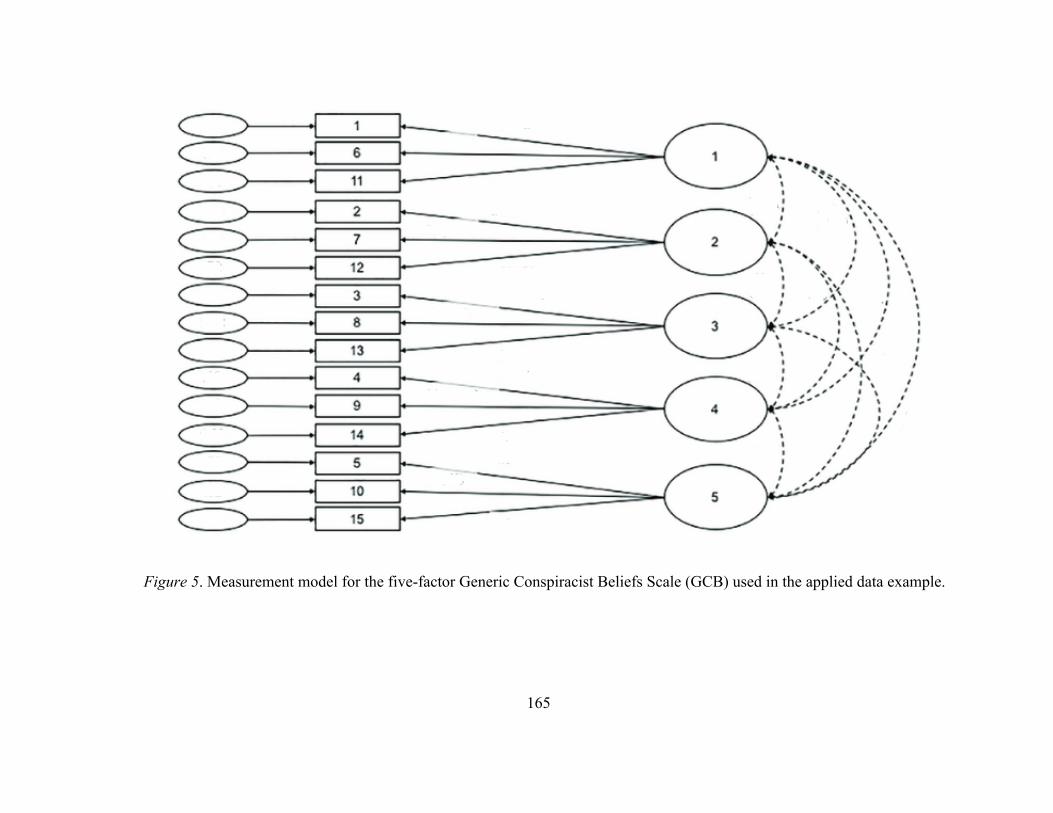
165
Figure 5. Measurement model for the five-factor Generic Conspiracist Beliefs Scale (GCB) used in the applied data example.