EUTROPHICATION – IMPLICATIONS OF N & P Intent of this lecture? • Link our discussions of terrestrial N & P dynamics with its

influences on receiving water bodies • How the relative amounts of N & P can influence the

growth and type of algae • Making the connection between chemical pollution and

biological problems Lecture based on –

Val H. Smith – Cultural eutrophication of inland, estuarine, and coastal waters. In Successes, Limitations and Frontiers in Ecosystem Science. M. L. Pace & P. M. Groffman (Editors), Springer Verlag, NY. 1998. Pgs 7-49. And Aquatic Pollution – Edward Laws This article highlights the important milestones in eutrophication research and provides an up to date discussion of N & P controls Natural versus Cultural Eutrophication Cultural – accelerated by anthropogenic activities

1

Introduction – brief history • Productivity of water bodies – research initiated in Europe

– work of Einar Naumann (Sweden) and August Theinemann (Germany)

• Naumann – developed the Trophic State Concept –

o Phytoplankton production determined by

concentrations of nitrogen and phosphorus o Productivity of lakes varied with the geological

characteristics of the watersheds • Naumann also developed the terms that we use to

categorize lakes based on their productivity and nutrient supplies

1. OLIGOTROPHIC 2. MESOTROPHIC 3. EUTROPHIC 4. HYPEREUTROPHIC

2

Mean values for the trophic classification system Condition Total P

(µg L-1) Chlorophyll a

(µg L-1) Secchi disk depth (m)

Ultra-Oligotrophic <4 <1 >12 Oligotrophic <10 <2.5 >6 Mesotrophic 10-35 2.5-8 6-3

Eutrophic 35-100 8-25 3-1.5 Hypereutrophic >100 >25 <1.5

3

4

5

6

Eutrophication studies began in the 1940s and published work peaked in the 1980s / 90s. These studies were conducted via – • Comparative analyses of different water bodies over time

and space, and • Experimentation at three different scales –

1. small-scale flask experiments such as bio-assays 2. medium-scale experiments such as mesocosms 3. whole-system manipulations (whole-lake experiments)

7

Nitrogen & Phosphorus as limiting nutrients First important development in eutrophication research – identification of N & P Driven by Leibig’s Law of the Minimum (1855)– The yield of a given species should be limited by the nutrient that was present in the least quantity in the environment relative to its demands for growth Variables for eutrophication – • Sunlight • Silica • N • P

Leibig’s law – resulted in the concept of nutrient limitation for algal growth –

1. a single nutrient should be the primary limiting factor for algal growth

2. observed algal growth should be proportional to the supply of the limiting nutrient

3. Practical control of the growth of algae can be accomplished via restricting the supply of the nutrient.

8

N & P were identified as the primary limiting nutrients -- this recognition was arrived at primarily by using bioassays. Other approaches used –

Physiological indicators

Elemental ratios – the ratio of N and P concentrations in the vegetation

Redfield (1958) – proposed that – the nutrient content of living algal cells can be given by a – • 7:1 by mass for N:P, or • elemental ratio of 16:1 for N:P

-- referred to as the Redfield ratio Given mass ratio, how would you compute the elemental ratio? This concept was extended to determine N & P controls If N:P supply > Redfield ratio – P limiting If N:P supply < Redfield ratio – N limiting However later work – showed that algae are composed of many species with varying N:P ratio (3 – 30)– and thus a single ratio was not very effective in determining N or P limitation

9

This variability was evident in Sakamoto’s (1966) results • when TN:TP < 10:1 – N limitation • when TN:TP > 17:1 – P limiting • between 10:1 17:1 – either N or P

What implications does this have?

10

Nutrient Loading Models (2nd important development) • Development of mass budgets for N & P for water bodies

and the linkage of input/outputs with waterbody concentrations –

• Initially received with considerable skepticism;

Thienemann remarked – that the concept “had nothing to do with limnology”.

• Vollenweider, Reckhow and Chapra – leading

proponents of the mass balance approach

• Mass balance approaches since then have become a cornerstone of ecosystem science research

• Models are based on the hydraulic characteristics of the

water body – depth, flow rate, length, etc. – factors that

11

determine the residence time or turnover time of the waterbody

• P models have received most of the attention. Example of

P model – TP – in lake P concentration (mg/m3)

82.0

155.1

⎥⎥⎦

⎤

⎢⎢⎣

⎡

+=

w

in

tPTP

where Pin is the mean annual P concentration in inflow, and tw is the residence time (yrs) how would you compute the residence time of a lake? Compared to N, P models have also been easier to formulate – why? Also we have had more success in formulating mass balance models for freshwater systems than marine systems -- difficult to identify boundaries of marine water bodies; considerable mixing of waters

12

Effects of nutrients on aquatic systems 3rd important development – Linking nutrient concentrations to – water quality variables of concern – e.g., algal biomass, water clarity, etc.

• Our perception/classification of eutrophication for

freshwater and marine waters varies! – NOTE lower thresholds (chlorophyll, clarity) for marine waters

13

• The controls that N and P have for eutrophication also varies with these waters

• Most of the freshwater lakes and reservoirs are limited by P • Strong relationships have been found between the

concentrations of P and algal mass (measured sometimes as the chlorophyll-a content)

Figure 2.1 - data for phytoplankton – floating algae in water bodies

2 observations from the figure – • hyperbolic relationship with P, with decreasing algal yields

beyond TP > 100 mg/m3

14

• Figure also indicates the shifts in limiting nutrient

(becomes N limited) as P concentration increases • Similar controls of P for periphyton (algae attached to

substrate) in streams and rivers have also been observed

periphyton in Scajaquada Creek in Buffalo (2002). • Figure 2.2

15

• Suspended algae in streams – also show P influences.

These algae originate from periphyton.

suspended algae in Scajaquada Creek in Buffalo (2002)

16

• However the mass of suspended algae in streams at a given level of P is much lower than the equivalent biomass of phytoplankton in lakes

17

In contrast, in marine systems the phytoplankton biomass is more tied to the N concentrations – suggesting that these systems are N-limited Why? Likely reasons –

1. P sequestration by Fe and Al oxides in freshwater systems 2. Fe and Mo availability for N-fixing bacteria in freshwater

systems (Fe and Mo are very low in marine waters) 3. High losses of N due to denitrification in marine waters

However, some studies (Hecky & Kilham, 1988) have shown that N-limitation may not be applicable always. Inability to define a well contained system has also limited a more thorough understanding of the N and P controls on marine phytoplankton

18

N & P Mixing – issues of stratification and overturning

Stratification of the lake because of the water temperature gradients during seasons Stratification occurs because of the variation in the density of water with temperature

- water most dense at 4 degree C - less dense above and below 4 degree C

19

Mixing is limited to specific zones Surface mixing occurs in the epilimnion – maybe 1m deep in summer or as much as 100 m under destabilized conditions. Epilimnion water will not mix with the hypolimnion when stratification is in place. After summer - When surface water temperatures cool up – reach 4 degree C – the surface water sinks – causes mixing and overturning! --- Fall Overturn If surface temps drop below 4C, again stratification will take place

20

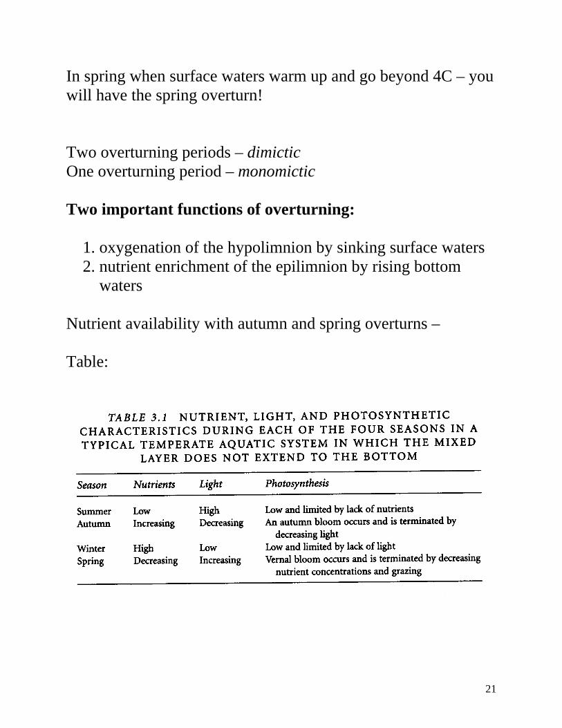
In spring when surface waters warm up and go beyond 4C – you will have the spring overturn! Two overturning periods – dimictic One overturning period – monomictic Two important functions of overturning:

1. oxygenation of the hypolimnion by sinking surface waters 2. nutrient enrichment of the epilimnion by rising bottom

waters Nutrient availability with autumn and spring overturns – Table:

21

Susceptibility of water bodies to O2 depletion: Deep oligotrophic systems do NOT suffer depletion – • Low productivity in epilimnion – respiratory rates not high

enough • The large depth of hypolimnion provides more than enough

O2 to meet any likely demands Shallow eutrophic systems – do not develop seasonal depletion – because the mixing layer extends to the bottom But – shallow eutrophic systems may develop – low O2 conditions overnight under no wind or calm weather conditions (when the mixing mechanism is shut off) --- example – the shallow western basin of Lake Erie Eutrophic systems with intermediate depths – most likely to be seasonally depleted by O2 - hypolimnion is small in depth - high production in the epilimnion - e.g., - central basin of Lake Erie. Seasonal depletions of O2 – do not cause mass die off’s of fish and aquatic species – it’s the overnight O2 depressions that do!

22

Salinity gradients can also affect mixing/stratification

• Occurs in estuaries – e.g, the Chesapeake Bay.

• May occur in conjunction with the temperature gradients

and make the scenario even worse. • In the Chesapeake Bay – increased inflows of freshwater –

make the O2 depletion condition worse. • Increasing urbanization (impervious surfaces) are expected

to increase flows.

23

Chesapeake Bay – N and P limitations Vary with season! Late winter/early spring – greatest outflows in the bay. Runoff rich in N – from fertilizer applications Most severe phytoplankton blooms occur in late winter/spring N:P ratio of water can be as high - 90:1 P limiting conditions! Summer – Runoff from watersheds is lowest Internal P release from bottom sediments due to bacterial decomposition N:P ratio of bay water can be as low as – 5:1 N limits phytoplankton growth! Hypoxia in the bay – number of factors – • Nutrients

24

• Freshwater runoff in spring • Oysters – shell fish – filter feeders of bacteria (bacteria

responsible too for oxygen depletion!)

25

N & P influences on phytoplankton community structure • The relative concentrations of N & P not only effect the

biomass but can also cause shifts in the species type • Cynobacteria blooms have been associated with N limiting

conditions (Cynobacteria are bacteria with chlorophyll and NOT a class of algae)

cynobacteria mass

o Problem with cynobacteria – is that these species produce potent toxins that impact other aquatic species

o Cynobacteria have also been found under excessive

eutrophic conditions – figure 2.6

26

• The resource-ratio theory has been used to explain the appearance of cynobacteria under N limiting conditions

o Resource-ratio theory – supplies of N, P, and silicon

and light are important determinants of algal species composition

• Under N limiting conditions – cynobacteria that are better

N scavengers than other species, out-compete the other algal species. Blue-green algae can fix their own N!

27

• This relationship is highlighted in Figure 2.7 (relative cynobacterial biomass increases for lower N:P ratios)

Implications of low N:P for plankton type????

28

Management Implications for N:P ratio loadings Virginia Coastal Plain Example – BMP implementation decreased the N:P ratio of exports from the watershed – much more needs to be done for P control

0.0 2.0 4.0 6.0 8.0 10.0

ammon-N

nitrate-N

soluble-org-N

particulate-N

ortho-P

soluble-org-P

particulate-P

total-N

total-P

loads (kg/ha)

pre-BMPpost-BMP

29

0

2

4

6

8

10

12

14

16

18

QN1

N:P

ratio pre-BMP

post-BMP

NOTE: elemental N : P ratio

30