european plant phenology and climate as seen in a 20-year avhrr

European plant phenology and climate as seen in a 20-year AVHRRland-surface parameter dataset

R. STOCKLI* and P. L. VIDALE

Institute for Atmospheric and Climate Science, ETH, Winterthurerstrasse 190,8057 Zurich, Switzerland

(Received 9 September 2002; in final form 26 May 2003 )

Abstract. Vegetation distribution and state have been measured since 1981 bythe AVHRR (Advanced Very High Resolution Radiometer) instrument throughsatellite remote sensing. In this study a correction method is applied to thePathfinder NDVI (Normalized Difference Vegetation Index) data to create acontinuous European vegetation phenology dataset of a 10-day temporal and0.1‡ spatial resolution; additionally, land surface parameters for use inbiosphere–atmosphere modelling are derived. The analysis of time-series fromthis dataset reveals, for the years 1982–2001, strong seasonal and interannualvariability in European land surface vegetation state. Phenological metricsindicate a late and short growing season for the years 1985–1987, in addition toearly and prolonged activity in the years 1989, 1990, 1994 and 1995. These varia-tions are in close agreement with findings from phenological measurements atthe surface; spring phenology is also shown to correlate particularly well withanomalies in winter temperature and winter North Atlantic Oscillation (NAO)index. Nevertheless, phenological metrics, which display considerable regionaldifferences, could only be determined for vegetation with a seasonal behaviour.Trends in the phenological phases reveal a general shift to earlier (20.54 days year21)and prolonged (0.96 days year21) growing periods which are statisticallysignificant, especially for central Europe.

1. Introduction

Interactions between the land surface and the atmosphere include turbulent

heat, moisture, momentum and carbon exchanges, which can largely determine the

state of climate and its variations in the near-surface continental climate (Chen et al.

2001, Pielke 2001). In addition, vegetation physiology and phenology are very

sensitive to climate forcings through several feedback mechanisms at various

timescales (Bounoua et al. 1999). It is well known, for instance, that plants

assimilate carbon in the process of photosynthesis, while losing water through

transpiration (Sellers et al. 1997): the terrestrial water and carbon cycles are closely

linked by these processes. Keeling et al. (1996) examined CO2 records from the

Mauna Loa station from 1964 to 1994 and found that amplitudes in the yearly CO2

cycle (linked to vegetation activity) increased by 20%. They attributed those trends

International Journal of Remote SensingISSN 0143-1161 print/ISSN 1366-5901 online # 2004 Taylor & Francis Ltd

http://www.tandf.co.uk/journalsDOI: 10.1080/01431160310001618149

*Corresponding author; e-mail: [email protected]

INT. J. REMOTE SENSING, 10 SEPTEMBER, 2004,VOL. 25, NO. 17, 3303–3330

to increased assimilation by land vegetation, associated with anthropogenic global

climate change.

The timing of phenological events is affected by naturally changing local

environmental conditions as well as by biogeochemical factors like diseases, soil

moisture, nutrients and age of the individual plants (Menzel 2000). Many phenologicalphases used in biometeorology, such as leaf unfolding and leaf colouring, are primarily

driven by local climatic conditions, like temperature and snow cover during winter and

early spring. Ground-measured vegetation phenology has been studied since the 18th

century (Menzel 2000, Roetzer et al. 2000, Defila 2001): data from International

Phenological Gardens (IPG) from 1959 to 1996 and from wild plants inSwitzerland, show high sensitivity of vegetation dynamics to interannual climate

variations. These studies have recently been linked to the observed global warming.

Phenological events in spring are known to be especially sensitive to climatic

influences: in the IPG phenological records springs have advanced over 6.3 days

and autumn has been delayed by 4.5 days since the early 1960s.

The variability of vegetation state and function motivates the creation of high-resolution vegetation parameters varying dynamically over space and time. These

parameters can be used to model the complex soil–vegetation–atmosphere

interactions but also to assess the long-term changes in land use and vegetation

physiology over a large area. During the last two decades many efforts have been

made to better integrate land surface processes in climate modelling: Sellers et al.1997 and more recently Pielke 2001 provide thorough reviews of land surface

models used in climate research. These mathematical formulations have evolved

during the last two decades from simple abiotic relationships, e.g. the bucket model

(Manabe 1969), to sophisticated biogeochemical models like Simple Biosphere

Model (SiB) 2 (Sellers et al. 1996a) and Land Surface Model (LSM) (Bonan 1996),which include a treatment of leaf photosynthesis and CO2 exchange. While it is

possible to derive biophysical vegetation parameters for use in these models from

existing land cover surveys, published in the form of maps (Matthews 1983, DeFries

et al. 1998, Hansen et al. 2000, Loveland et al. 2000), this approach accounts

exclusively for spatial variability, neglecting temporal variability. The knowledge oftemporal variability of vegetation function is, however, a key issue to meet the

requirements of the United Nations Framework Convention on Climate Change

(UNFCCC) and the Kyoto Protocol, in order to quantify the carbon pools and

exchanges on local and on global scale.

The knowledge of vegetation phenology for entire ecosystems and on globalscale has thus in past decades been limited, either in space or in time. In comparison

to the ground-based global vegetation classifications by Matthews (1983) and

Wilson and Henderson-Sellers (1985), satellite remote sensing now offers the

possibility to estimate vegetation phenology on the global scale with a high

temporal frequency. Since the 1980s multi-spectral satellite observations from theNational Oceanic and Atmospheric Administration’s (NOAA) Polar Orbiting

Environmental Satellites (POES) provide daily global coverage datasets of visible

and near-infrared surface reflectances. From those, the Normalized Difference

Vegetation Index (NDVI) can be derived as has been shown by Justice et al. (1985),

Tucker and Sellers (1986), Reed et al. (1994), Voivy and Saint (1994), Myneni et al.(1997), Champeaux et al. (2000), Los et al. (2001) and Zhou et al. (2001). The

NDVI exploits the spectral properties of green plant leaves and is an estimator for

the radiation used within the photosynthesis process occurring in leaves. Asrar et al.

(1985), Tucker and Sellers (1986), Sellers et al. (1996b) and Los (1998) showed that

3304 R. Stockli and P. L. Vidale

the temporal evolution of the Fraction of Photosynthetically Active Radiation

absorbed by the green leaves (FPAR), the Leaf Area Index (LAI) and other

biophysical vegetation parameters can be estimated empirically from NDVI with

the use of land cover type dependent vegetation constants. Sets of land surface

parameters can be found of low resolution and global scale in the ISLSCP dataset

collection (Meeson et al. 1995) for the years 1987/1988, extended by Los et al.

(2000) for the 9-year period 1982–1990.

Satellite sensor data can also provide a good means to verify trends of ground

observed vegetation activity. Myneni et al. (1997) have investigated the 1981–1991

Advanced Very High Resolution Radiometer (AVHRR) NDVI record from the

GIMMS and the Pathfinder dataset for the northern hemisphere. They have

detected an advance in the active growing season of 8¡3 days and a delay in the

declining phase of 4¡2 days over this decade. Zhou et al. (2001) looked at the

northern hemisphere vegetation activity derived from AVHRR NDVI and land

surface temperature records during 1981–1998 and found an increase in mean

NDVI for Eurasia and North America.

Remote sensing of land surface properties is, however, a complex and pro-

blematic task. Atmospheric absorption and scattering by gas molecules and

aerosols, persistent cloud cover, viewing geometry effects, illumination conditions

and technical difficulties limit the use of these satellite measurements. Muchresearch has been accomplished in the last two decades in order to correct and

calibrate multi-temporal NDVI data (Tucker and Matson 1985, Holben 1986,

Goward et al. 1991, Gutman and Ignatov 1995, Cihlar et al. 1994, Sellers et al.

1996b, Los 1998, Los et al. 2000).

In this study we use the highly processed NOAA/NASA Pathfinder NDVI

dataset, which is already corrected for many of the problems mentioned above.

From the Pathfinder NDVI a continuous 20-year vegetation phenology dataset is

extracted and biophysical land surface parameters covering the period from 1982 to

2001 are derived with high spatial and temporal resolution. We focus on Europe and

study regional variability seen in vegetation dynamics. The methodology involves the

use of a refined correction algorithm based on Los et al. (2000) to extract the

vegetation phenology from satellite sensor data. Long-term surface observations in

both phenology and climate over continental Europe make it possible to conduct

meaningful statistical intercomparisons and this offers the opportunity to further

validate the soundness and usefulness of these land surface products. Inter-annual

variability and regional differences in phenology in particular have not been analysed

previously at this spatial and temporal scale over this region.

In §2 the methodology used to derive the set land surface parameters from the

NASA/NOAA Pathfinder NDVI is presented. An analysis of interannual and

seasonal variation of these land surface parameters is presented in the Results in §3.

The relationship between interannual climate anomalies and vegetation phenology

are examined for a number of European sub-domains. A discussion of the results

follows in §4.

2. Data and methodology

2.1. Pathfinder NDVI

The NDVI exploits the spectral properties of green plant leaves, which absorb

incoming radiation in the visible part of the spectrum (AVHRR red channel:

0.62–0.7 mm) and strongly reflect light in the near-infrared wavelengths (AVHRR

NIR channel: 0.74–1.1 mm). This ratio has low values ranging from 20.2 to z0.1

Plant phenology and climate from AVHRR data 3305

for snow, bare soil, glaciers, rocks and rises to around 0.2–0.8 for green vegetation.

NDVI is an estimator for the radiation used within the photosynthetic processes

occurring in leaves.

For the derivation of the 1982–2001 biophysical surface parameters we used the

NOAA/NASA Pathfinder NDVI dataset (James and Kalluri 1994). The data are

collected by the AVHRR instrument onboard the NOAA POES platforms. These

operational satellites are successively replaced at failure and are supposed to

provide a continuous and consistent data record into the future. The Pathfinder

NDVI dataset is corrected for Rayleigh scattering by applying the radiative transfer

model by Gordon et al. (1988). Ozone absorption in the signal is removed by the

estimation of the atmospheric ozone column from daily TOMS (Total Ozone

Mapping Spectrometer) measurements. Each satellite (NOAA 7, 9, 11 and 14—only

the ‘afternoon’ overpass satellites were used by the Pathfinder project) flown during

the period 1981 to present has been subject to instrumental degradation during the

operational period, which was accounted for by fitting a time-dependent calibration

algorithm (Rao and Chen 1996) for each individual channel. The NDVI is

calculated from the AVHRR channel 1 visible (VIS) and channel 2 near-infrared

(NIR) reflectances by taking the ratio

NDVI~NIR{VIS

NIRzVISð1Þ

Within the Pathfinder NDVI dataset these daily swath data are geolocated and

gridded at 8 km resolution and composited over 10-day periods with the maximum

value composite (MVC) algorithm (Holben 1986) to a global coverage. The dataset

is not corrected for aerosols (for instants volcanic eruptions such as Mt Pinatubo in

June 1991 or smoke from forest fires), water vapour absorption and illumination

and viewing geometry effects. Some of these disturbances are compensated in the

NDVI since it is basically a ratio between two spectral bands. Zhou et al. (2001)

assess the effect of the solar zenith angle to NDVI as weak, especially in seasonal

and inter-annual terms. An average registration error of 6 km was observed by

Holben (1986) in the geolocated AVHRR data. Prior to any corrections, an overall

absolute error in the NDVI in the order of 0.1–0.2 must be considered (Los 1998).

The lack of a good pre-calibration in the AVHRR Pathfinder NDVI dataset is

problematic for the derivation of spatio-temporally consistent land surface

parameters. For the generation of the 10-day composites the cloud mask is not

used. Also, anomalously high data values (NDVI w0.8) are found and pixels with

high solar zenith angles are set to missing data values. Yearly time-series of the

NOAA Pathfinder NDVI for various areas and years are found in figure 1 (thin

solid lines) and show some of the inconsistencies. More sophisticated atmospheric

correction schemes are used for the MODIS (MODerate resolution Imaging

Spectroradiometer) data processing (see, for example, Vermote et al. 1997).

The current in-operation POES afternoon satellite NOAA-14 is consistently

drifting westwards, which leads to a later equatorial overpass. In figure 2 time-series

of NDVI for the years 1981–2001 are shown. Over the Sahara desert (figure 2(a))

the higher solar zenith and instrument angles leads to a decreasing NDVI signal

beginning in late 2000. For vegetated areas this effect is partly compensated as

this can be seen in figure 2(b), but the degradation of the satellite signal is

problematic for our application, since northern Europe will have larger data

dropouts during winter time. The NASA DAAC does not recommend using

the newest 2001 Pathfinder data for scientific purposes (http://daac.gsfc.nasa.gov/


CAMPAIGN_DOCS/LAND_BIO/AVHRR_News.html) and has stopped produ-

cing the dataset on a regular basis by September 2001. A new generation of sensors

like MODIS (launched onboard the TERRA satellite in 1999 and onboard the

AQUA satellite in 2002) can provide land surface data for this time period.

Figure 1. Pathfinder NDVI time-series (thin solid), Fourier adjusted with an unweightedscheme (dotted), weighted after Sellers et al. (1996b) (dashed) and with the EFAI-NDVI method discussed in this paper (thick solid). (a) Swiss Alps, (b) Finland, (c)Norway, (d ) Finland, (e) north-west France, ( f ) Sicily, (g) Ireland, and (h) Sweden.


2.2. Correction methodology

To create a consistent dataset of vegetation phenology, we analyse and correct

yearly time-series of Pathfinder NDVI over the European continent at a 10-day

temporal and 0.1‡ spatial grid for the period from 1982 to 2001. Two steps are involved

in the spatio-temporal interpolation process: (1) replacement of processing artefacts

and no-data values in the dataset by spatial interpolation (§2.3.); and (2) adjustment of

the NDVI time-series by using a temporal interpolation procedure (§2.4.).

The following three assumptions can be made when extracting time-series of the

state of land surface vegetation from the error-contaminated satellite remotely

sensed NDVI:

. The vegetation phenology follows a repetitive seasonal cycle (Moulin et al.

1997) and NDVI values vary smoothly with time (Sellers et al. 1996b).

. During the summer, outliers in NDVI time-series are the result of either cloud

cover or atmospheric disturbances. These effects tend to decrease NDVI

values (Holben 1986, Los 1998).. During the winter, snow under or temporarily on the canopy may impose a

negative bias on the NDVI signal, since snow has a high VIS reflectance and a

low NIR reflectance.

These assumptions lead to the application of a Fourier adjustment algorithm

described in Sellers et al. (1996b) and Los (1998). The second-order Fourier series

are able to represent the seasonal variability of vegetation phenology with a smooth

analytical function and the original data can be weighted so that higher NDVI

values representing uncontaminated measurements receive higher weights than

negative outliers (which are attributed to erroneous measurements). This technique

was applied successfully to produce the FASIR-NDVI (Fourier Adjustment, Solar

zenith angle, correction, Interpolation and Reconstruction) published in the ISLSCP

dataset collection (Meeson et al. 1995) at a monthly temporal and 1‡ spatial scale.

The following sections present the modifications brought to the Sellers et al. (1996b)

Figure 2. Twenty-year NDVI time-series for a grid point in (a) the Sahara and(b) the Alps. The dashed line shows the original Pathfinder NDVI, and the solidline represents the corrected EFAI-NDVI phenology time-series.


and Los (1998) approach in order to create the new 0.1‡ and 10-day EFAI-NDVI

(European Fourier-Adjusted and Interpolated NDVI) dataset.

2.3. Spatial interpolation

In comparison to the ISLSCP FASIR-NDVI the present dataset is of a much

higher spatio-temporal resolution and therefore small area inconsistencies in the

dataset are well visible. We have applied a spatial interpolation prior to extracting

the yearly phenology curves from the NDVI time-series. No-data values in high

latitude biomes during winter are set to a minimum NDVI value as it is a pre-

requisite for the correct functioning of the temporal interpolation described in §2.4.

To remove the most predominant artefacts all NDVI values above 0.8 are set to

missing data. A second-order Fourier series, f, is fitted to the yearly Pathfinder NDVI

time-series at each grid point. Anomalous NDVI values are detected and flagged

as missing if they were outside the boundary (0.8f20.2)vNDVIv(1.2fz0.2) of

this ‘idealized’ phenology curve f. Missing data are spatially interpolated for each

10-day interval according to the following technique, which is an inverse-distance

weighted interpolation. For each missing grid point valid neighbours of the same

land cover class within a radius r are sampled. The missing value is then replaced by

an inverse distance weighted mean of these valid neighbours:

Wi~1ffiffiffiffiffiffiffiffiffiffiffiffiffiffi

x2i zy2

i

q ð2Þ

NDVI~

P

WiNiP

Wi

ð3Þ

where Wi~weight of a valid neighbour Ni, xi~horizontal distance of neighbour Ni

to the missing value, yi~vertical distance of neighbour Ni to the missing value,

Ni~valid neighbouring NDVI, same land cover class as the missing NDVI value.

Missing data in high latitudes during winter time do occur in an extended area

and cannot be interpolated by the above described method. They are flagged when

missing data are found for successively five or more 10-day intervals during winter

for an individual grid point. Using a land cover map (DeFries et al. 1998) these

prolonged periods of missing data are replaced differently for deciduous and for

evergreen vegetation. During winter deciduous vegetation is assumed to be in a

dormant state and the canopy may be masked by snow cover. These grid points are

assigned to a NDVI value of 20.05. Boreal conifers found in Sweden, Finland and

the former Soviet Union keep their needles during winter. They project out of the

snow layer and these areas have a low albedo during winter (Betts and Ball 1997).

All NDVI values for evergreen forests, which are lower than 0.25 are replaced by

the mean of the four last valid NDVI values in late autumn (mostly October

values). The underlying assumption of this method holds when NDVI for evergreen

forests does not drop below the chosen threshold and if by the end of the vegetation

period all deciduous plants have shed their leaves (Sellers et al. 1996b).

Spatial error detection and interpolation is applied to all of the 10-day Pathfinder

datasets over the European domain ranging from August 1981 until July 2001.

2.4. Temporal interpolation

The production of NDVI-derived biophysical parameters, used in LSMs to

drive the yearly evolution of land surface vegetation, requires that for each grid


point they are consistent over time and represent the actual area-averaged state of

vegetation. According to the three assumptions presented at the beginning of this

section the second order Fourier series are used to extract the seasonal varying

phenology time-series from the spatially interpolated NDVI dataset. The Fourier

adjustment technique performs well, as described in Sellers et al. (1996b) and Los

(1998). We evaluate the Fourier adjustment algorithm by first working with

theoretical time-series of simulated yearly NDVI curves including artificial data

gaps. In figure 3 we compare the use of 10-day intervals (36 yearly data values) to

monthly time-steps. The use of 10-day intervals enhances the ability of the Fourier

adjustment to reproduce the simulated phenological curve, even when 2 months of

data are flagged as missing. In figure 3(b) the reconstructed curve has a better fit to

the original curve with R2~0.994 for 10-day intervals than for a monthly dataset

(figure 3(a), R2~0.922). Especially during the start and the end of the active

growing period the temporal resolution seems to be an important factor.

Nevertheless, the original Fourier adjustment algorithm as first described by

Sellers et al. (1996b) has several shortcomings when used with the 0.1‡ and 10-day

Pathfinder NDVI. Biomes with a short growing season have a steep increase in

Figure 3. Theoretical phenology time-series: (a) 12 and (b) 36 data values per year. Thesolid line represents the modelled NDVI time-series with a 2-month long gap periodwhere a discrete Fourier time-series (dashed) was fitted.


photosynthetic activity in late spring due to leaf unfolding and snowmelt and are

subject to a rapid decrease in NDVI when they shed their leaves in autumn. Only a

short period of greenness is observed for those biomes (high latitude deciduous

forest and biomes in mountainous regions). Second-order Fourier series are able to

represent features of a half-year periodicity and cannot account for such fast

processes. As a result, the state of vegetation can be overestimated by the Fourier

adjustment at the beginning and at the end of the growing season and in some cases

a second peak is simulated in late winter. The Fourier adjustment algorithm is

developed for spatially and temporally subsampled data at the 1‡61‡ level and

works well with that configuration. The present dataset is at a much finer resolution

and includes local-scale variability and short term features (e.g. leaf-out in spring)

due to the used 10-day interval.

The ideas developed by Sellers et al. (1996b) and Los (1998) are revised for our

purposes and only modifications to these algorithms presented here. For each grid

point, yearly NDVI time-series are processed in the following way:

1. Each yearly time-series is tested for a summertime growing season. The

temporal derivative of a fitted second-order Fourier series is examined for each year

at each pixel. A growing season is detected if the maximum/minimum derivative of

this modelled curve f exceeds 0.03/20.03 for the start/end of the growing season

(corresponding to an increase/decrease of 0.03 (NDVI) per 10 days). The actual

start/end dates of the growing season is then shifted one 10-day period to the

beginning/end of the year to be on the safe side. Only deciduous vegetation classes

are tested for a growing season.

2. For vegetation with a continuous transition between the growing/non-

growing period (e.g. evergreen biomes) we apply the weighted Fourier adjustment

procedure proposed by Los (1998) with a slightly modified weighting function. This

new weighting function is shown in figure 4 and does prevent excessive weights for

large positive anomalies in the time-series.

W~d{tð Þ{t

� �4

, t vd v0

4ffiffiffi

dp

z1, d¢0

8

<

:

ð4Þ

where t~–0.1, d~NDVI-f, NDVI~spatially corrected NDVI values, f~second-

order discrete Fourier series of NDVI, and W~weights

Figure 4. Weighting scheme used for the weighted Fourier adjustment procedure: (dashed)weighting scheme by Sellers et al. (1996b) and (solid) weighting scheme applied in thisstudy.


3. For vegetation with a dormant and an active state in the vegetation

phenology the weighted Fourier adjustment procedure is only applied to the

growing season. The weighting scheme is modified as follows:

growing season: W~d{tð Þ{t

� �4

, t vd v0

4ffiffiffi

dp

z1, d¢0

8

<

:

ð5Þ

dormant period: W~1:0 ð6ÞThe non-weighted Fourier series f is used during the dormant period and the

weighted series during the growing season, thus both the weighted and the

unweighted Fourier series are merged at the two phenological transition dates. This

way the curve still inherits the seasonal periodicity of the growth cycle.

The Pathfinder NDVI dataset is processed by applying the steps 1–3 to the

whole European domain, using data from August 1981 until July 2001. A yearly

time-series over the Swiss Alps in figure 1(a) (thick solid line) shows that the

beginning and the end of the growing season are identified precisely due to the high

temporal resolution and the modified weighting scheme. In figure 1(b) an anomaly

found at the end of the growing season in the original Pathfinder NDVI is

eliminated by the spatial interpolation. There is an advantage in using separate

corrections for the growing and the non-growing season, which can be seen in

figure 1(c): second-order Fourier series do not represent well growing seasons

shorter than half a year (dashed line) and merging the separate corrections at the

phenological transition dates (thick solid line) catches the onset and the offset of the

growing season. In figure 1(d ) a yearly time-series of an evergreen vegetation type

mostly found in the northern European boreal zone is displayed and figure 1(e)

shows evergreen vegetation in the north-western coast of France. A different

seasonal behaviour with signs of dryness-related vegetation stresses is seen in

figure 1( f ) for southern European vegetation. However, not all time-series have

been processed correctly: in figure 1(g) an unrealistic seasonal behaviour was

created for a point in Ireland. Nevertheless the long and early growing season is a

well known feature in Ireland, due to the influence of the NAD (North Atlantic

Drift), and is represented well. In figure 1(h) an example is displayed where the

growing season was not determined correctly.

The resulting dataset has been named EFAI-NDVI (European Fourier-Adjusted

and Interpolated NDVI). It is a highly corrected dataset of European vegetation

phenology covering the last two decades.

2.5. Deriving biophysical parameters from the EFAI-NDVI

Remotely sensed parameters like the EFAI-NDVI are not directly applicable in

LSMs. The parameters needed by modern LSMs usually consist of a number of

vegetation type-dependent static look-up values (like root depth or canopy height) and

time-dependent parameters which describe the phenological evolution of the plants.

Static parameter look-up tables by vegetation type can be found in the literature

(Dickinson 1984, Sellers et al. 1996a,b) and will have a spatial distribution when

combined with vegetation type maps (Hansen et al. 2000, Loveland et al. 2000). The

most commonly used time-varying parameters include LAI, canopy greenness and z0

(roughness length). More sophisticated models like SiB 2 make use of the FPAR

parameter to scale leaf photosynthesis to the ecosystem level.


We derive a number of biophysical land surface parameters from the previously

generated EFAI-NDVI dataset. They include FPAR, LAI, z0 and canopy greenness

and are derived following the publication by Los (1998) by simple empirical

relationships which have been verified and updated in various field observations

(FIFE, OTTER, BOREAS and HAPEX-Sahel, see references in Los 1998, Los et al.

2000). The theoretical background to the derivation of these biophysical land

surface parameters can be reviewed in Sellers et al. (1996b), Los (1998) and the

most basic relationships are presented in the Appendix. Examples of these land

surface parameters are shown in figures 5 and 6.

In figure 5, a justification for the high temporal resolution of this dataset is

found: the three maps show the LAI in the Alps region for the compositing periods

of 1–10 May (a), 11–20 May (b) and 21–31 May (c). During this month a large

increase in LAI is observed in southern Germany, eastern Austria but also in the

alpine valleys of Switzerland. The use of monthly composites would mask many of

these short term phenology changes.In figure 6 the land surface parameters are illustrated for the time period of

10–21 July. FPAR has a very homogeneous pattern and shows high values over most of

central, eastern and northern Europe during summer, where LAI exhibits a more

spatially varying pattern, especially between tall forest vegetation and short ground-

cover in Scandinavia. A very dense vegetation with high LAI values is seen in most of

eastern Europe. Roughness length has an exponential scaling with LAI and heavily

depends on the canopy height. It clearly shows the distribution of short vegetation (low

z0 ranging from 5 to 20 cm) and tall tree biomes (high z0 between 1 and 3 m).

3. Spatial and temporal variability of European vegetation related to climate

Spatial and temporal variability found in the land surface parameters is

discussed in this section. We will mostly use the EFAI-NDVI as the primary

parameter and not the derived land surface parameters. The derived land surface

parameters inherit the same seasonal and interannual variability, since they are

first-order dependent on the EFAI-NDVI and only second-order on land cover (see

§2). Statistics in this section are either calculated for the full Europe domain or for

sub-domains. In figure 7 the geographical extents of the chosen sub-domains are

illustrated. This sub-domain system does not reflect any bio-geographical

stratification found in literature but is a first step to isolate and analyse the data

by regional domains, also in view of the intended future applications of this dataset.

It includes a longitudinal gradient from maritime (UK and Ireland) to continental

(Western Russia) and a latitudinal gradient from the Alps to Northern Europe. The

Mediterranean (e.g. Spain) is not included since the analysis procedure in this

section requires a large seasonal amplitude in the phenology. The Alps are analysed

separately since this area is of special interest for our research in regional climate.

3.1. Seasonal variability

Land surface vegetation is often classified into ecosystem types, the so-called

biomes. Each such biome represents a community of plants in a certain climatic

zone and can also be characterized by its specific phenological evolution throughout

the year. Phenological events within a biome may include flowering, leafing,

dryness-periods, harvesting (for agriculture biomes) and leaf-fall. The timing of


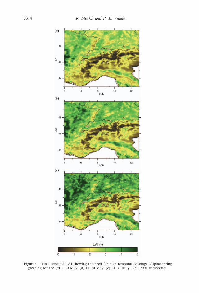
Figure 5. Time-series of LAI showing the need for high temporal coverage: Alpine springgreening for the (a) 1–10 May, (b) 11–20 May, (c) 21–31 May 1982–2001 composites.


these events is dependent on internal plant physiological factors and external

influences like plant diseases and local climate.

In figure 8, phenological curves derived from the EFAI-NDVI and averaged by

Figure 6. Maps of the derived land surface parameters covering the period from 10 to21 July (average yearly climatology derived from the years 1982–2001). (a) FPAR,(b) LAI and (c) z0.


land cover class (SiB land cover classification, derived from the DeFries et al. 1998

land cover classification, see table A1) are shown on the left side. The distribution

of NDVI values are displayed for each land cover class on the right side.

Deciduous forest types (figure 8(a), (b) and (d)) can clearly be distinguished from

evergreen forest (figure 8(c)) which is mostly found in the boreal zone and in alpine

areas. In total, tall tree biomes account for 10.1% of the examined land surface.

The evergreen pine trees keep their needles in winter and the seasonal variation is

due to the deciduous plants found in those forests. Mixed and deciduous forests

(figure 8(b)) found in intermediate and high latitudes have a large seasonal variabi-

lity, with low NDVI values in winter and high values in summer, also visible in the

NDVI distribution diagrams (right column of figure 8).

The shrub and bare soil biome (figure 8(e))—covering 13.8% of the area—is

found in the Mediterranean and is subject to a dry climate which does not allow the

growth of tall trees. This fact is well reflected in the phenological curve of this

biome, where even a reduced greenness in summer due to possible drought

conditions is visible. Tundra vegetation (figure 8( f )) is only present in 0.1% of the

examined land surface area but the usually short vegetation period and low

temperatures for this biome are reflected in the phenology curve, which does not

reach high values even in July/August.

The soil/desert landcover class (figure 8(g)) is not subject to much vegetation

activity, as expected. A rapid and early increase in NDVI is seen in the agriculture

Figure 7. The sub-domain extents that were used to derive anomalies and trends in the EFAI-NDVI dataset.

Figure 8. Yearly phenology time-series averaged by land cover class (left) and distributionsof NDVI values for these curves (right). The time-series (solid lines) are plotted withtheir standard deviation (dashed lines) for each land cover class.


biome (figure 8(h)) with a gradual decrease after June. Agricultural land is in fact

the biome with the largest area coverage found in Europe (24.9%)

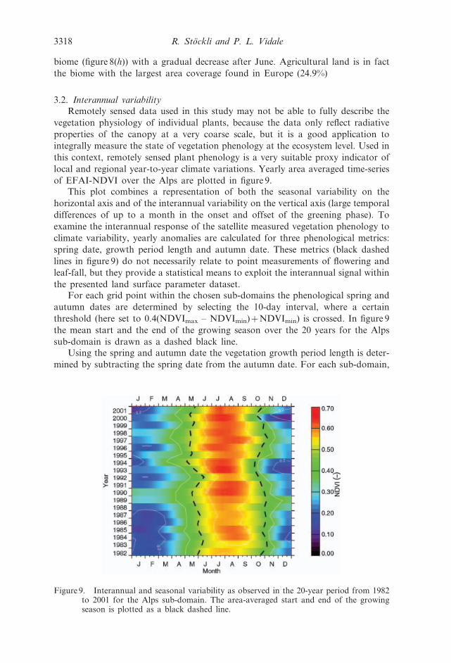
3.2. Interannual variability

Remotely sensed data used in this study may not be able to fully describe the

vegetation physiology of individual plants, because the data only reflect radiative

properties of the canopy at a very coarse scale, but it is a good application to

integrally measure the state of vegetation phenology at the ecosystem level. Used in

this context, remotely sensed plant phenology is a very suitable proxy indicator of

local and regional year-to-year climate variations. Yearly area averaged time-series

of EFAI-NDVI over the Alps are plotted in figure 9.This plot combines a representation of both the seasonal variability on the

horizontal axis and of the interannual variability on the vertical axis (large temporal

differences of up to a month in the onset and offset of the greening phase). To

examine the interannual response of the satellite measured vegetation phenology to

climate variability, yearly anomalies are calculated for three phenological metrics:

spring date, growth period length and autumn date. These metrics (black dashed

lines in figure 9) do not necessarily relate to point measurements of flowering and

leaf-fall, but they provide a statistical means to exploit the interannual signal within

the presented land surface parameter dataset.For each grid point within the chosen sub-domains the phenological spring and

autumn dates are determined by selecting the 10-day interval, where a certain

threshold (here set to 0.4(NDVImax – NDVImin)zNDVImin) is crossed. In figure 9

the mean start and the end of the growing season over the 20 years for the Alps

sub-domain is drawn as a dashed black line.

Using the spring and autumn date the vegetation growth period length is deter-

mined by subtracting the spring date from the autumn date. For each sub-domain,

Figure 9. Interannual and seasonal variability as observed in the 20-year period from 1982to 2001 for the Alps sub-domain. The area-averaged start and end of the growingseason is plotted as a black dashed line.


all successfully determined phenological metrics are averaged to form a regional

scale time-series of spring dates, autumn dates and growth period lengths for the

years 1982–2001.

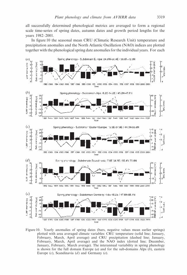
In figure 10 the seasonal mean CRU (Climatic Research Unit) temperature and

precipitation anomalies and the North Atlantic Oscillation (NAO) indices are plotted

together with the phenological spring date anomalies for the individual years. For each

Figure 10. Yearly anomalies of spring dates (bars, negative values mean earlier springs)plotted with area averaged climate variables: CRU temperature (solid line; January,February, March, April average) and CRU precipitation (dashed line; January,February, March, April average) and the NAO index (dotted line; December,January, February, March average). The interannual variability in spring phenologyis shown for the full domain Europe (a) and for the sub-domains Alps (b), easternEurope (c), Scandinavia (d ) and Germany (e).


sub-domain the spring dates are compared with winter (January, February, March,

April) temperature/precipitation anomalies and to the winter NAO indices (December,

January, February, March). The NAO is a very relevant climatic index for Europe.

Strong positive phases of the NAO tend to be associated with above-normal tem-peratures across Northern Europe and below-normal temperatures in Greenland

and often across southern Europe and the Middle East. They are also associated

with above-normal precipitation over northern Europe and Scandinavia and below-

normal precipitation over southern and central Europe. Opposite patterns of tem-

perature and precipitation anomalies are typically observed during strong negative

phases of the NAO. The wintertime NAO, in particular, exhibits significant

interannual and decadal variability (Hurrel 1995).

The full European domain (figure 10(a)) was subject to early springs in the years1989 and 1990 as well as the years 1994 and 1995 and 2000. A positive winter NAO

phase and warmer spring temperatures in 1989/1990 and in 1994/1995 are a possible

indication of the continental scale climate influence on the observed greening

pattern. The early 1980s were generally late years in phenological terms. Lower

winter temperatures as well as a negative NAO index (normally leading to colder

winters and springs and also to extended snow cover) can have caused delayed

spring greenings of land surface vegetation during the period 1982–1987. In

figure 11, phenological anomalies are correlated with climatic anomalies. The toprow of figure 11 displays anomalies in spring phenology correlated to temperature,

precipitation and NAO index anomalies. For Europe, winter temperatures are

negatively correlated with the timing of plant-growth in spring (figure 11(a)). No

significant correlation with precipitation is found (figure 11(b)) but the winter

NAO—a proxy for the general weather pattern over continental Europe—is weakly

linked to spring phenological timing (figure 11(c)). In elevated terrain and at high

latitudes plant growth in spring is known to be temperature limited and—because

of the high soil moisture availability—not highly dependent on precipitation. Springevents such as needle flush and leaf unfolding are found in biometeorology to be

very sensitive to spring and winter temperatures (Farquhar et al. 1980, Post and

Stenseth 1999, Menzel 2000, Defila 2001).

The Alps (figure 10(b)) do not show anomalously early springs in the years 1989/

1990 and 1995. Over this sub-domain we generally find late springs in the 1980s and

early springs in the 1990s. Apart from effects on plant growth related to

topography, the southern and eastern ridge of the Alps are known to be strongly

influenced by Mediterranean climate, which can lead to a significant difference inthe plant phenology to the one observed in the northern ridge (Defila 2001) and

may also explain some of the difference between the Alps and the rest of Europe. In

the second row of figure 11, we correlate spring temperature anomalies with spring

phenology for different sub-domains. The correlation of spring anomalies with the

observed winter/spring temperatures for the Alps sub-domain (figure 11(d )) is rather

weak compared with, for example, eastern Europe (figure 11(e)) and Scandinavia

(figure 11( f )).

Spring anomalies for eastern Europe are plotted in figure 10(c) and show verylarge interannual variability. No strong decadal pattern (1980/1990s) like in the

Alps is observed but rather the years 1989/1990, 1994/1995 and the most recent

years 1997–2001 are exhibiting very early springs of up to 25 days earlier than the

mean spring date. The negative correlation of eastern European spring phenology

with temperature anomalies is also high, with a value of 0.789 (figure 11(e)).

Phenology in the Scandinavian sub-domain (figure 10(d )) has a temporal pattern


similar to the full European domain. The growing season had an exceptionally early

start in the years 1989/1990 and did not show reasonable difference from the mean

in the years 1994–1998. Generally, the decadal pattern of late springs in the 1980s

is also visible in Scandinavia, but the same pattern is much more pronounced

in western central Europe (figure 10(e)). Early leaf-out in Scandinavia is strongly

linked with positive temperature deviations in winter/spring over that area

(figure 11( f )).

Interannual variability of plant phenology is also observed on the ground in a

sophisticated and long-term network of phenological gardens (IPG—International

Phenological Gardens) around the globe. Menzel (2000) has collected and analysed

observational data from the IPGs in Europe for the years 1959–1996. In this dataset

the same years as observed in the EFAI-NDVI show an early spring with more

Figure 11. Phenological metrics (spring date, autumn date and vegetation period length) arecorrelated to temperature, precipitation and the NAO index in different sub-domains.


than a week difference compared with the 1976–1980 spring dates. The growing

season was observed to be anomalously long throughout the period from 1989 until

1995, which was partly reproduced in this study. In our dataset the years 1989/1990

and 1994/1995 have early springs but years 1991–1993 show a rather nominal to

late spring. It is well known in phenology research that the leaf-out in spring is

easier to measure than the autumn date. In our dataset, autumn dates are likely to

be affected by persistent cloud cover and data dropouts in winter. The third row of

figure 11 correlates phenological metrics in different seasons to temperature

anomalies. The autumn phases do not correlate well with spring temperatures

(figure 11(i)). Also, summer temperature (figure 11( j)), precipitation (figure 11(k)) or

NAO data (figure 11(l)) anomalies are only correlating weakly with R2~0.330,

0.199 and 0.065. These simple relationships cannot account for the complex soil–

vegetation–atmosphere interactions during the summer months, especially for the

long term soil-moisture memory related effects. For most sub-domains the growth

period length has a positive (but weak) correlation with spring temperatures.

Since 1951, phenological data from wild grown plant species have been collected

systematically in Switzerland. A number of plant species at different biogeogra-

phical locations are observed and phenological phases are recorded by lay observers

and data are processed at MeteoSwiss. Defila (1996, 2001) has analysed the aver-

aged time-series for spring and autumn events for Switzerland covering the years

1951–1995. Interannual variations of these observations show a good agreement

with our phenology data. The overall picture of Switzerland indicates an excep-

tionally early spring in 1990 and 1994 (up to 20 days) and late growing seasons for

the period 1985–1987. The metrics for the Alps and Germany (figure 10(b),(e)) show

a similar temporal pattern, although the years 1989 and 1990 are somewhat less

pronounced (4–7 days earlier spring) than in 1994 (20 days earlier).

3.3. Multi-year trends

Error sources in the remotely sensed NDVI products may be a serious limitation

to the detection of anthropogenic trends in land surface vegetation. The non-

adequate calibration of the used Pathfinder NDVI dataset described in §2 can lead

to errors of the same order of magnitude as the observed trends in NDVI. Also,

existing satellite measurements cover a relatively short time period. It is important

to keep these limitations in mind while working with trend analysis of NDVI time-

series. Satellite remote sensing is nevertheless the only feasible means that we have

to observe the long term biospheric activity with a large area coverage.

In our dataset we assume that trends are due to changes in canopy reflectance

properties, thus only occurring in vegetated areas. Trends detected in deserted areas

can be attributed to systematic instrumental drifts. The mean EFAI-NDVI trend in

a deserted region (Sahara 0.2‡E–2.6‡E, 29.3‡N–31.1‡N) is 0.21% year21. Mean

NDVI trends for vegetated areas are significantly higher and range from 0.9 to

1.5% year21, which supports the reliability of trends in vegetated areas.

We apply linear regression analysis to our NDVI time-series and check for

trends in spring date, growth period length, autumn date, minimum NDVI,

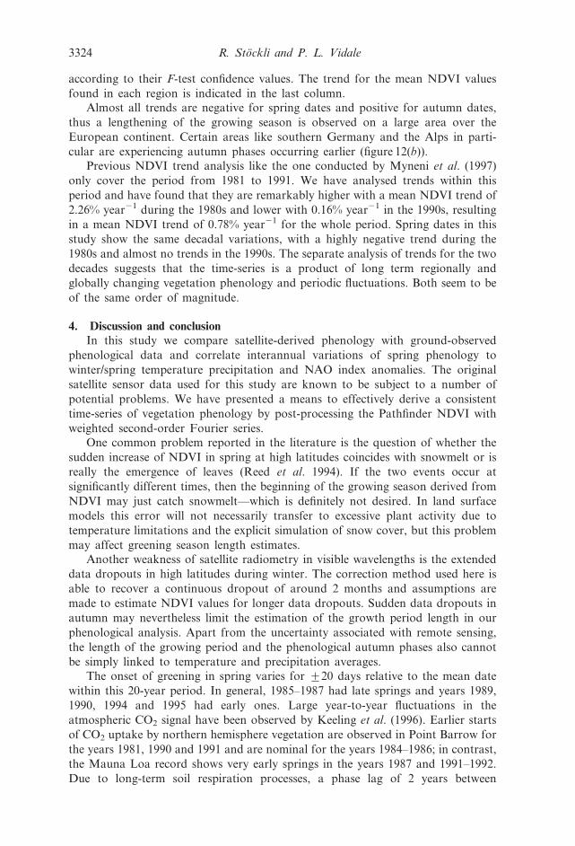
maximum NDVI and mean NDVI. Maps of Europe with spring and autumn date

trends are shown in figure 12. The results reveal evidence for long-term changes in

the European plant phenology. Central Europe seems to exhibit a general earlier

appearance of plants in spring during the last 20 years, whereas northern Europe

shows the opposite trend.


An average of the trends is calculated for the individual sub-domains in Europe.

The trends of the phenological metrics are only calculated for grid points where a

growth period was observed and phenological dates can actually be determined. In

table 1, spring, autumn and growing season length trends given and classified

Figure 12. Multi-year trends found in the spring (a) and the autumn dates (b).

Table 1. Trends in European phenology derived from the EFAI-NDVI dataset.

RegionSpring

(days year21)Autumn

(days year21)Length

(days year21)NDVI

(% year21)

Germany 21.41{ 20.04* 1.38{ 0.85Alps 21.53 20.69* 0.84* 0.74Scandinavia 20.48* 0.44* 0.92* 0.82Eastern Europe 21.32{ 0.30* 1.63* 1.12Western Russia 20.47* 0.61* 1.08* 0.79UK and Ireland 21.88{ 0.51* 2.38* 0.84Iceland 20.44* 0.37* 0.81* 1.26Middle East 20.48* 0.49* 0.97* 0.72

Europe (full domain) 20.54* 0.42* 0.96{ 0.78

Significance level: *1%, {5%, {10%.


according to their F-test confidence values. The trend for the mean NDVI values

found in each region is indicated in the last column.

Almost all trends are negative for spring dates and positive for autumn dates,

thus a lengthening of the growing season is observed on a large area over the

European continent. Certain areas like southern Germany and the Alps in parti-

cular are experiencing autumn phases occurring earlier (figure 12(b)).

Previous NDVI trend analysis like the one conducted by Myneni et al. (1997)

only cover the period from 1981 to 1991. We have analysed trends within this

period and have found that they are remarkably higher with a mean NDVI trend of

2.26% year21 during the 1980s and lower with 0.16% year21 in the 1990s, resulting

in a mean NDVI trend of 0.78% year21 for the whole period. Spring dates in this

study show the same decadal variations, with a highly negative trend during the

1980s and almost no trends in the 1990s. The separate analysis of trends for the two

decades suggests that the time-series is a product of long term regionally and

globally changing vegetation phenology and periodic fluctuations. Both seem to be

of the same order of magnitude.

4. Discussion and conclusion

In this study we compare satellite-derived phenology with ground-observed

phenological data and correlate interannual variations of spring phenology to

winter/spring temperature precipitation and NAO index anomalies. The original

satellite sensor data used for this study are known to be subject to a number of

potential problems. We have presented a means to effectively derive a consistent

time-series of vegetation phenology by post-processing the Pathfinder NDVI with

weighted second-order Fourier series.

One common problem reported in the literature is the question of whether the

sudden increase of NDVI in spring at high latitudes coincides with snowmelt or is

really the emergence of leaves (Reed et al. 1994). If the two events occur at

significantly different times, then the beginning of the growing season derived from

NDVI may just catch snowmelt—which is definitely not desired. In land surface

models this error will not necessarily transfer to excessive plant activity due to

temperature limitations and the explicit simulation of snow cover, but this problem

may affect greening season length estimates.

Another weakness of satellite radiometry in visible wavelengths is the extended

data dropouts in high latitudes during winter. The correction method used here is

able to recover a continuous dropout of around 2 months and assumptions are

made to estimate NDVI values for longer data dropouts. Sudden data dropouts in

autumn may nevertheless limit the estimation of the growth period length in our

phenological analysis. Apart from the uncertainty associated with remote sensing,

the length of the growing period and the phenological autumn phases also cannot

be simply linked to temperature and precipitation averages.

The onset of greening in spring varies for ¡20 days relative to the mean date

within this 20-year period. In general, 1985–1987 had late springs and years 1989,

1990, 1994 and 1995 had early ones. Large year-to-year fluctuations in the

atmospheric CO2 signal have been observed by Keeling et al. (1996). Earlier starts

of CO2 uptake by northern hemisphere vegetation are observed in Point Barrow for

the years 1981, 1990 and 1991 and are nominal for the years 1984–1986; in contrast,

the Mauna Loa record shows very early springs in the years 1987 and 1991–1992.

Due to long-term soil respiration processes, a phase lag of 2 years between


atmospheric CO2 anomalies and vegetation–climate anomalies is proposed by

Keeling et al. (1996), which makes their results consistent with our analysis.

The knowledge of these interactions has led to the assumption that global land

use changes, anthropogenic emissions of greenhouse gases (CO2, methane) as wellas the observed global warming are possibly enhancing large area biospheric

activity. We find trends in the 20-year EFAI-NDVI that generally agree with recent

findings in plant phenology research. Linear trends of the averaged EFAI-NDVI

time-series vary from 0.72 to 1.12% per year depending on the region. These trends

indicate an overall enhanced vegetation activity, mostly due to a prolongation of the

growing season with earlier occurring springs for the whole Europe (20.54 days year21).

Regional differences are visible. The trends are more pronounced in Germany

(1.41 days year21) than they are in Scandinavia (20.48 days year21) where we also findevidence for delayed springs. The quantitatively small trends which are extracted

from the satellite-measured vegetation phenology are, however, approximately of

the same order of magnitude as the expected errors in the dataset. Moreover, the

methodology presented here cannot replace and, in fact, requires a good pre-

calibration of satellite sensor data, which is not available in the Pathfinder dataset.

We believe that further research, longer NDVI time-series, ground validation and

especially an in-depth cross-calibration with new satellite sensors (the MODIS

instrument onboard TERRA and AQUA), and long-term ground measurements ofphenological data are needed to gain more confidence.

Developing this methodology was useful in order to prepare for the arrival of

MODIS data. The dataset has shown to be useful at this resolution and does agree

with known European climatic zone characteristics in both space and time.

Generally, the results increase our confidence in the usefulness of satellite sensor

derived land surface parameters for land surface modelling. These parameters

inherit seasonal and interannual dynamics seen in land surface vegetation over the

last two decades. They are a good estimator for large-scale plant photosynthesis

and phenology but they cannot account for many of the factors that drive landsurface processes (such as soil moisture availability, nutrients availability and

vapour pressure deficit). Only the use of these land surface parameters in a land

surface model which is coupled to a climate model (e.g. the CHRM regional climate

model, Vidale et al. 2003) will enable us to study the full spectrum of the complex

soil–vegetation processes and land–atmosphere feedbacks. An upcoming paper will

explore the application of this dataset in regional climate modelling.

AcknowledgmentsThe funding for this study was provided by the National Centre of Competence

in Research on climate variability, predictability, and climate risks (NCCR) funded

by the Swiss National Science Foundation (NSF). The authors would like to

first express their thanks for the support and suggestions of Professor Christoph

Schar.

We would like to thank Sietse O. Los, Jim Collatz and Jim Tucker for

discussions and data and would like to acknowledge ETH and Code 912/913 at

Goddard Space Flight Center for being able to use their computing resources,which were essential for the successful completion of this project. Special thanks

go to Scott Denning, Kevin Schaefer and Ian Baker from CSU for providing

access to the mapper code used to process the derived biophysical land surface

parameters.

The Land Pathfinder NDVI data used in this study were produced through


funding from the Earth Observing System Pathfinder Program of NASA’s Mission

to Planet Earth in cooperation with the National Oceanic and Atmospheric

Administration. The data were provided by the Earth Observing System Data and

Information System (EOSDIS), Distributed Active Archive Center at Goddard

Space Flight Center, which archives, manages and distributes this dataset.

We highly encourage the use of the presented biophysical land surface

parameters as a climatology (1982–2001) or as a 20-year time-series. This dataset is

designed for and capable of enhancing existing LSMs with a boundary condition

allowing the representation of spatial and temporal dynamics of land surface

vegetation. The parameter set is available from the authors upon request.

Appendix

The basic relationships between NDVI and the most common land surface

parameters are reviewed in this section.

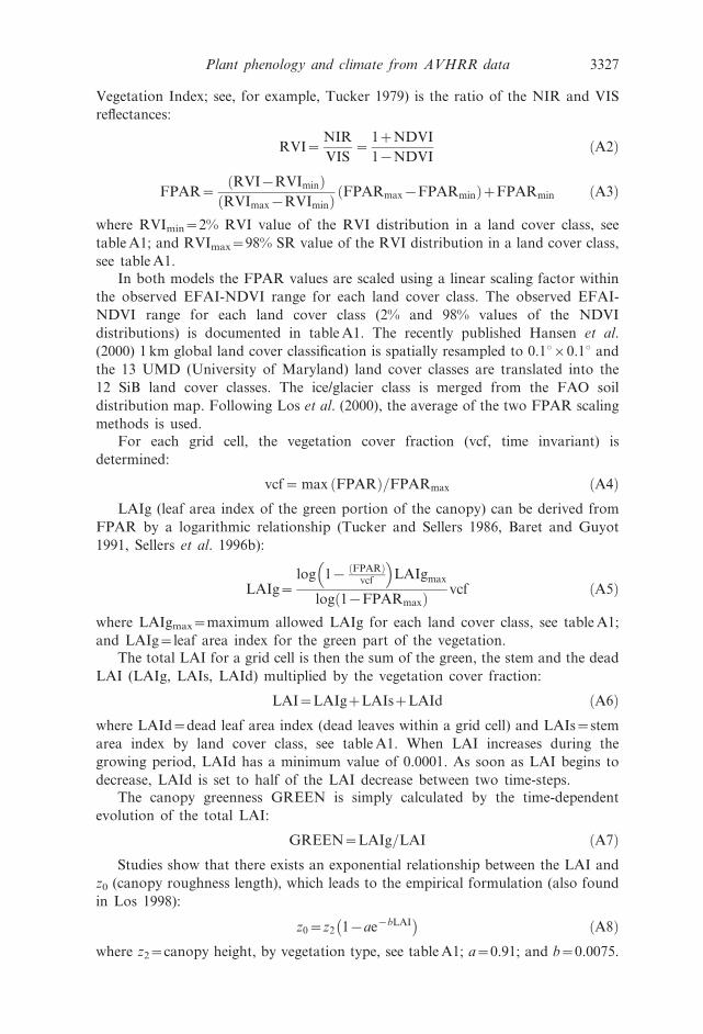
Dye and Goward (1993) and Sellers et al. (1996b) show that FPAR has a linear

relationship with NDVI:

FPAR~NDVI{NDVIminð Þ

NDVImax{NDVIminð Þ FPARmax{FPARminð ÞzFPARmin ðA1Þ

where NDVImin~2% NDVI value of the NDVI distribution in a land cover class,

see table A1; NDVImax~98% NDVI value of the NDVI distribution in a land cover

class, see table A1; FPAR~Fraction of Photosynthetically Active Radiation

absorbed by the green leaves of the canopy; FPARmax~0.95; and FPARmin~0.01.Los et al. (2000) also use the RVI–FPAR relationship, where RVI (Ratio

Table A1. DeFries et al. (1998)—SiB land cover reclassification with NDVI-FPAR scalingvalues.

ClassSiB

ClassUMD

Dominant vegetationtype

%Cover NDVImin NDVImax LAImax LAIs

z2

(m)

0 0 Ocean and inland water – – – – – –1 2 Broadleaf evergreen trees{ – – – 7 0.08 35.02 4 Broadleaf deciduous trees 0.4 0.008 0.766 7 0.08 20.03 5 Broadleaf and needleleaf

trees4.4 20.015 0.757 7.5 0.08 20.0

4 1 Needleleaf evergreen trees 5.3 20.102 0.742 8 0.08 17.05 3 Needleleaf deciduous trees 0.0 20.039 0.734 8 0.08 17.06 6 Broadleaf and groundcover 7.4 20.031 0.734 5 0.05 1.07 7 Grassland and shrub cover 9.3 20.055 0.718 5 0.05 1.08 – Shrubs and groundcover{ – – – 5 0.05 1.09 8, 9 Broadleaf shrubs with bare

soil13.8 20.039* 0.695* 5 0.05 0.5

10 13 Tundra 0.1 20.023 0.688 5 0.05 0.611 12 Bare soil and desert 21.3 20.039* 0.695* 5 0.05 1.012 10, 11 Agriculture and grasslands 24.9 20.039 0.695 6 0.05 1.013 – Ice§ 12.9 20.039* 0.695* 5 0.01 –

*These values were taken from the SiB Grassland class, since NDVI for these vegetationtypes does not rise to a maximum FPAR.

{There are no broadleaf evergreen trees (tropical rainforest) in the processed Europeandomain.

{For this SiB land cover class, no appropriate UMD class is found.§The Ice class was merged from the FAO Digital Soil Map of the World (FAO 1995).


Vegetation Index; see, for example, Tucker 1979) is the ratio of the NIR and VIS

reflectances:

RVI~NIR

VIS~

1zNDVI

1{NDVIðA2Þ

FPAR~RVI{RVIminð Þ

RVImax{RVIminð Þ FPARmax{FPARminð ÞzFPARmin ðA3Þ

where RVImin~2% RVI value of the RVI distribution in a land cover class, see

table A1; and RVImax~98% SR value of the RVI distribution in a land cover class,

see table A1.

In both models the FPAR values are scaled using a linear scaling factor within

the observed EFAI-NDVI range for each land cover class. The observed EFAI-

NDVI range for each land cover class (2% and 98% values of the NDVI

distributions) is documented in table A1. The recently published Hansen et al.

(2000) 1 km global land cover classification is spatially resampled to 0.1‡60.1‡ and

the 13 UMD (University of Maryland) land cover classes are translated into the

12 SiB land cover classes. The ice/glacier class is merged from the FAO soil

distribution map. Following Los et al. (2000), the average of the two FPAR scaling

methods is used.

For each grid cell, the vegetation cover fraction (vcf, time invariant) is

determined:

vcf~ max FPARð Þ=FPARmax ðA4ÞLAIg (leaf area index of the green portion of the canopy) can be derived from

FPAR by a logarithmic relationship (Tucker and Sellers 1986, Baret and Guyot

1991, Sellers et al. 1996b):

LAIg~log 1{

FPARð Þvcf

� �

LAIgmax

log 1{FPARmaxð Þ vcf ðA5Þ

where LAIgmax~maximum allowed LAIg for each land cover class, see table A1;

and LAIg~leaf area index for the green part of the vegetation.

The total LAI for a grid cell is then the sum of the green, the stem and the dead

LAI (LAIg, LAIs, LAId) multiplied by the vegetation cover fraction:

LAI~LAIgzLAIszLAId ðA6Þwhere LAId~dead leaf area index (dead leaves within a grid cell) and LAIs~stem

area index by land cover class, see table A1. When LAI increases during the

growing period, LAId has a minimum value of 0.0001. As soon as LAI begins to

decrease, LAId is set to half of the LAI decrease between two time-steps.

The canopy greenness GREEN is simply calculated by the time-dependent

evolution of the total LAI:

GREEN~LAIg=LAI ðA7ÞStudies show that there exists an exponential relationship between the LAI and

z0 (canopy roughness length), which leads to the empirical formulation (also found

in Los 1998):

z0~z2 1{ae{bLAI� �

ðA8Þwhere z2~canopy height, by vegetation type, see table A1; a~0.91; and b~0.0075.


References

ASRAR, G., KANEMASU, E. T., JACKSON, R. D., and PINTER, P. J., 1985, Estimation of totalabove-ground phytomass production using remotely sensed data. Remote Sensing ofEnvironment, 17, 211–220.

BARET, F., and GUYOT, G., 1991, Potentials and limits of vegetation indexes for LAI andAPAR assessment. Remote Sensing of Environment, 35, 161–173.

BETTS, A. K., and BALL, J. H., 1997, Albedo over the boreal forest. Journal of GeophysicalResearch, 102, 28 901–28 909.

BONAN, G. B., 1996, A land surface model (LSM version 1.0) for ecological, hydrological,and atmospheric studies: technical description and user’s guide. NCAR TechnicalNote, NCAR/TN-417zSTR, National Center for Atmospheric Research, Boulder,Colorado.

BOUNOUA, L., COLLATZ, G. J., SELLERS, P. J., RANDALL, D. A., DAZLICH, D. A., LOS, S. O.,BERRY, J. A., FUNG, I., TUCKER, C. J., FIELD, C. B., and JENSEN, T. G., 1999,Interactions between vegetation and climate: radiative and physiological effects ofdoubled atmospheric CO2. Journal of Climate, 12, 309–324.

CHAMPEAUX, J.-L., ARCOS, D., BAZILE, E., GIARD, D., GOUTORBE, J.-P., HABETS, F.,NOILHAN, J., and ROUJEAN, J.-L., 2000, AVHRR-derived vegetation mapping overWestern Europe for use in numerical weather prediction models. InternationalJournal of Remote Sensing, 21, 1183–1199.

CHEN, F., PIELKE, R. A., and MITCHELL, K., 2001, Development and application of land-surface models for mesoscale atmospheric models: problems and promises. WaterScience and Application, 3, 107–135.

CIHLAR, J., MANAK, D., and VOISIN, N., 1994, AVHRR bidirectional reflectance effects andcompositing. Remote Sensing of Environment, 48, 77–88.

DEFILA, C., 1996, 45 years phytophenological observations in Switzerland, 1951–1995.Proceedings of 14th International Congress of Biometeorology 1–8 September 1996,Ljubljana, Slovenia, edited by A. Hoeevar, Z. Repineek and L. Kajfe-Bogataj,Biometeorology, Volume 14, pp. 175–183.

DEFILA, C., 2001, Phytophenological trends in Switzerland. International Journal ofBiometeorology, 45, 203–207.

DEFRIES, R. S., HANSEN, M., TOWNSHEND, J. R. G., and SOLBERG, R., 1998, Global landcover classification at 8 km spatial resolution: the use of training data derived fromLandsat imagery in decision tree classifiers. International Journal of Remote Sensing,19, 3141–3168.

DICKINSON, R. E., 1984, Modelling evapotranspiration for three-dimensional global climatemodels. In Climate Processes and Climate Sensitivity, edited by J. E. Hansen andT. Takehashi, (Washington, DC: American Geophysical Union), 29, pp. 58–72.

DYE, D. G., and GOWARD, S. N., 1993, Photosynthetically active radiation absorbed byglobal land vegetation in August 1984. International Journal of Remote Sensing, 14,3361–3364.

FARQUHAR, G. D., CAEMMERER, S. V., and BERRY, J. A., 1980, A biochemical model ofphotosynthetic CO2 assimilation in leaves of C3 species. Planta, 149, 78–90.

FAO (FOOD AND AGRICULTURE ORGANIZATION), 1995, A Digital Soil Map of the World.CD-ROM, Land and Water Development Division, FAO, Rome, Italy.

GORDON, H. R., BROWN, J. W., and EVANS, R. H., 1988, Exact Rayleigh scattering calculationsfor use with the Nimbus-7 coastal zone color scanner. Applied Optics, 27, 2111–2122.

GOWARD, S. N., MARKHAM, B., DYE, D. G., DULANEY, W., and YANG, J., 1991,Normalized Difference Vegetation Index measurements from the Advanced VeryHigh Resolution Radiometer. Remote Sensing of Environment, 35, 257–277.

GUTMAN, G. G., and IGNATOV, A., 1995, Global land monitoring from AVHRR: potentialsand limitations. International Journal of Remote Sensing, 16, 2301–2309.

HANSEN, M. C., DEFRIES, R. S., TOWNSHEND, J. R. G., and SOHLBERG, R., 2000, GlobalLand cover classification at 1 km spatial resolution using a classification treeapproach. International Journal of Remote Sensing, 21, 1331–1364.

HOLBEN, B. N., 1986, Characteristics of maximum-value composite images for temporalAVHRR data. International Journal of Remote Sensing, 7, 1435–1445.

HURREL, J. W., 1995, Decadal trends in the NAO. Science, 269, 676–679.JAMES, M. E., and KALLURI, S. N. V., 1994, The Pathfinder AVHRR land dataset: an


improved coarse resolution dataset for terrestrial monitoring. International Journal ofRemote Sensing, 15, 3347–3363.

JUSTICE, C. O., TOWNSHEND, J. R. G., HOLBEN, B. N., and TUCKER, C. J., 1985, Thephenology of global vegetation using meteorological satellite data. InternationalJournal of Remote Sensing, 6, 1271–1318.

KEELING, C. D., CHIN, J. F. S., and WHORF, T. P., 1996, Increased activity of northernvegetation inferred from atmospheric CO2 measurements. Nature, 382, 146–149.

LOS, S. O., 1998, Linkages between global vegetation and climate: an analysis based onNOAA-Advanced Very High Resolution Radiometer Data. PhD Dissertation, VrijeUniversiteit, Amsterdam.

LOS, S. O., COLLATZ, G. J., SELLERS, P. J., MALMSTROM, C. M., POLLACK, N. H., DEFRIES,R. S., BOUNOUA, L., PARRIS, M. T., TUCKER, C. J., and DAZLICH, D. A., 2000, Aglobal 9-year biophysical land surface dataset from NOAA AVHRR data. Journal ofHydrometeorology, 1, 183–199.

LOS, S. O., COLLATZ, G. J., BOUNOUA, L., SELLERS, P. J., and TUCKER, C. J., 2001, Globalinterannual variations in sea surface temperature and land surface vegetation, airtemperature, and precipitation. Journal of Climate, 14, 1535–1549.

LOVELAND, T. R., REED, B. C., BROWN, J. F., OHLEN, D. O., ZHU, Z., YANG, L., andMERCHANT, J. W., 2000, Development of a global land cover characteristics databaseand IGBP DISCover from 1 km AVHRR data. International Journal of RemoteSensing, 21, 1303–1330.

MANABE, S., 1969, Climate and the ocean circulation: 1. The atmospheric circulation and thehydrology of the earth’s surface. Monthly Weather Review, 97, 739–805.

MATTHEWS, E., 1983, Global vegetation and land use: new high-resolution data bases forclimate studies. Journal of Climate and Applied Meteorology, 22, 474–487.

MEESON, B. W., CORPREW, F. E., MCMANUS, J. M. P., MYERS, D. M., CLOSS, J. W., SUN,K.-J., SUNDAY, D. J., and SELLERS, P. J., 1995, ISLSCP Initiative I: Global DataSets for Land–Atmosphere Models, 1987–1988, vols 1–5. CD ROM, NASA GoddardDAAC, Greenbelt, USA.

MENZEL, A., 2000, Trends in phenological phases in Europe between 1951 and 1996.International Journal of Biometeorology, 44, 76–81.

MOULIN, S., KERGOAT, L., VOIVY, N., and DEDIEU, G., 1997, Global-scale assessment ofvegetation phenology using NOAA/AVHRR satellite measurements. Journal ofClimate, 10, 1154–1170.

MYNENI, R. B., KEELING, C. D., TUCKER, C. J., ASRAR, G., and NEMANI, R. R., 1997,Increased plant growth in the northern high latitudes from 1981–1991. Nature, 386,698–702.

PIELKE, R. A., 2001, Earth system modeling—an integrated assessment tool forenvironmental studies. In Present and Future of Modeling Global EnvironmentalChange: Toward Integrated Modeling, edited by T. Matsuno and H. Kida (Tokyo:Terrapub), pp. 311–337.

POST, E., and STENSETH, N. C., 1999, Climatic variability, plant phenology, and northernungulates. Ecology, 80, 1322–1339.

RAO, C. R., and CHEN, J., 1996, Post-launch calibration of the visible and near-infraredchannels of the Advanced Very High Resolution Radiometer on the NOAA-14spacecraft. International Journal of Remote Sensing, 17, 2743–2847.

REED, B. C., BROWN, J. F., VANDERZEE, D., LOVELAND, T. R., MERCHANT, J. W., andOHLEN, D. O., 1994, Measuring phenological variability from satellite imagery.Journal of Vegetation Science, 5, 703–714.

ROETZER, T., WITTENZELLER, M., HAECKEL, H., and NEKOVAR, J., 2000, Phenology incentral Europe—differences and trends of spring phenophases in urban and ruralareas. International Journal of Biometeorology, 44, 60–66.

SELLERS, P. J., RANDALL, D. A., COLLATZ, G. J., BERRY, J. A., FIELD, C. B., DAZLICH,D. A., ZHANG, C., and BOUNOUA, L., 1996a, A revised land surface parameterization(SiB2) for GCMs. Part 1: Model formulation. Journal of Climate, 9, 676–705.

SELLERS, P. J., LOS, S. O., TUCKER, C. J., JUSTICE, C. O., DAZLICH, D. A., COLLATZ, G. J.,and RANDALL, D. A., 1996b, A revised land surface parameterization (SiB2) foratmospheric GCMs. Part 2: The generation of global fields of terrestrial biophysicalparameters from satellite data. Journal of Climate, 9, 706–737.

SELLERS, P. J., DICKINSON, R. E., RANDALL, D. A., BETTS, A. K., HALL, F. G., BERRY,


J. A., COLLATZ, G. J., DENNING, A. S., MOONEY, H. A., NOBRE, C. A., SATO, N.,FIELD, C. B., and HENDERSON-SELLERS, A., 1997, Modeling the exchanges of energy,water, and carbon between continents and the atmosphere. Science, 275, 502–509.

TUCKER, C. J., 1979, Red and photographic infrared linear combinations for monitoringvegetation. Remote Sensing of Environment, 8, 127–150.

TUCKER, C. J., and MATSON, M., 1985, Determination of volcanic dust deposition of ElChichon from ground and satellite data. International Journal of Remote Sensing, 6,619–627.

TUCKER, C. J., and SELLERS, P. J., 1986, Satellite remote sensing of primary production.International Journal of Remote Sensing, 7, 1395–1416.

VERMOTE, E. F., EL SALEOUS, N., JUSTICE, C. O., KAUFMAN, Y. J., PRIVETTE, J. L.,REMER, L., ROGER, J. C., and TANRE, D., 1997, Atmospheric correction of visibleand middle-infrared EOS-MODIS data over land surfaces: background, operationalalgorithm and validatation. Journal of Geophysical Research, 102, 17 131–17 141.

VIDALE, P. L., LUETHI, D., FREI, C., SENEVIRATNE, S., and SCHAER, C., 2003, Predictabilityand uncertainity in a regional climate model. Journal of Geophysical Research,108(D18), 4586.

VOIVY, N., and SAINT, G., 1994, Hidden Markov models applied to vegetation dynamicsanalysis using satellite remote sensing. IEEE Transactions on Geoscience and RemoteSensing, 32, 906–917.

WILSON, M. F., and HENDERSON-SELLERS, A., 1985, A global archive of land cover and soilsdata for use in general circulation models. Journal of Climatology, 5, 119–143.

ZHOU, L., TUCKER, C. J., KAUFMANN, R. K., SLAYBACK, D., SHABANOV, N. V., andMYNENI, R. B., 2001, Variations in northern vegetation activity inferred fromsatellite data of vegetation index during 1981 to 1999. Journal of GeophysicalResearch, 106, 20 069–20 083.

3330 Plant phenology and climate from AVHRR data

european plant phenology and climate as seen in a 20-year avhrr

Documents