ESTIMATION, VALIDATION, AND FORECASTS OF REGIONAL COMMERCIAL MARINE VESSEL

INVENTORIES Final Report

Submitted by James J. Corbett, P.E., Ph.D.

Jeremy Firestone University of Delaware

Coauthored by Chengfeng Wang, Ph.D.

ARB Contract Number 04-346 CEC Contract Number 113.111

Prepared for the California Air Resources Board

and the California Environmental Protection Agency and for

the Commission for Environmental Cooperation of North America

5 April 2007

i

Disclaimer The statements and conclusions in this Report are those of the contractor and not necessarily those of the California Air Resources Board. The mention of commercial products, their source, or their use in connection with material reported herein is not to be construed as actual or implied endorsement of such products.

ii

Acknowledgments This work received partial funding from the Commission for Environmental Cooperation

(CEC) project number 113.111. This work also benefited from significant in-kind support from members of the North American SOx Emission Control Area (SECA) team and their contractors. In particular, this work was shared with Research Triangle Institute (RTI), at the direction of the United States Environmental Protection Agency (U.S. EPA) and ARB. RTI developed a trade-based model forecasting energy demand from commercial ships, and the forecasts described in this work are a product of coordination with this U.S. EPA-funded effort. Necessarily, we cite these communications in this study, although future work may cite the RTI report to U.S. EPA when that report can be referenced.

In particular, we thank John Callahan of the Research & Data Management Services of the University of Delaware for his help applying the GIS tools. We acknowledge with appreciation the significant review comments, and contributions by ARB staff (including Dongmin Luo, Todd Sax, Andy Alexis, Michael Benjamin, and Kirk Rosenkranz); the work greatly benefited from their guidance. We acknowledge collaborative discussions with the North American SECA team, including representatives of Environment Canada (Joanna Bellamy, Naomi Katsumi (who provided the Canada data), Patrick Cram, Andrew Green, Veronique Bouchet, and Morris Mennell), the Commission for Environmental Cooperation (Paul Miller, now at NESCAUM, who obtained the Mexico data on our behalf), and the U.S. Environmental Protection Agency (Barry Garelick, Penny Carey, and others). In addition, we acknowledge the work and review of fellow SECA contractors, including Brewster Boyd at Ross and Associates, Louis Browning at ICF, and Chris Lindhjem at Environ. We acknowledge the good work products and collaborative discussions regarding forecast results with Mike Gallagher and Martin Ross at RTI and with Dave St. Amand at Navigistics Consulting.

This Report was submitted in fulfillment of contract number 04-346, Estimation, Validation, and Forecasts of Regional Commercial Marine Vessel Inventories, by the University of Delaware under the partial sponsorship of the California Air Resources Board (ARB). Tasks 1 and 2 received partial funding from the Commission for Environmental Cooperation (CEC) project number 113.111, and significant in-kind support from member of the North American SOx Emission Control Area (SECA) team and their contractors. Work on Tasks 1 and 2 of the project was completed as of March 2006. Work on Tasks 3 and 4 of the project was completed as of October 2006. Project work was completed as of January 2007.

iii

Table of Contents Disclaimer ...................................................................................................................................................... i Acknowledgments.........................................................................................................................................ii Table of Contents.........................................................................................................................................iii List of Figures .............................................................................................................................................. iv List of Tables ............................................................................................................................................... iv ABSTRACT.................................................................................................................................................. v EXECUTIVE SUMMARY .........................................................................................................................vi 1.0 INTRODUCTION............................................................................................................................... 1

1.1 Purpose and Scope....................................................................................................................... 1 1.2 Project Background and Assumptions......................................................................................... 1 1.3 Previous Work ............................................................................................................................. 2

1.3.1 Inventory Development ...................................................................................................... 3 1.3.2 Trends and Forecasting ....................................................................................................... 4

2.0 MATERIALS AND METHODS........................................................................................................ 7 2.1 Baseline Conditions: STEEM description ................................................................................... 8 2.2 Rates of Change: Installed power as first-order trend indicator for CMV emissions................ 12

2.2.1 Evaluating coupled growth in cargo and energy............................................................... 13 2.3 Patterns of Change: First-order consideration at North American scale ................................... 14

3.0 RESULTS ......................................................................................................................................... 16 3.1 Baseline Emissions Estimates ................................................................................................... 16 3.2 Producing Spatially Resolved Emissions Inventories for Various Pollutants (Task 1)............. 18 3.3 Inventory Summary by Vessel Type ......................................................................................... 20 3.4 Comparison with Other Emissions Studies (Task 2) ................................................................. 20 3.5 Forecasting principles................................................................................................................ 23 3.6 Activity-based modeling of freight growth ............................................................................... 24

3.5.1 Growth Rates .................................................................................................................... 26 3.5.2 Growth Patterns ................................................................................................................ 29

3.7 Future Emissions without SECA region (Task 3) ..................................................................... 30 3.8 Future Emissions with Potential SECA (Task 4) ...................................................................... 31

4.0 DISCUSSION ................................................................................................................................... 33 4.1 Comparison with global forecast trends .................................................................................... 33 4.2 Uncertainty and Bounding......................................................................................................... 33

5.0 SUMMARY AND CONCLUSIONS................................................................................................ 35 5.1 Baseline Inventory..................................................................................................................... 35 5.2 Forecast Trends ......................................................................................................................... 36

6.0 RECOMMENDATIONS .................................................................................................................. 39 6.1 Improve precision ...................................................................................................................... 39 6.2 Reduce Base-Year Uncertainty ................................................................................................. 39 6.3 Improve Trend Extrapolation .................................................................................................... 39 6.4 Incorporate additional detail among drivers affecting change................................................... 41 6.5 Incorporate planned or proposed signals to modify technological change trends ..................... 41 6.6 Model fleet behavior in response to potential action................................................................. 41 6.7 Extend voyage data or analytical detail ..................................................................................... 41

7.0 REFERENCES.................................................................................................................................. 42 LIST OF ACRONYMS .............................................................................................................................. 48 Appendix: Summary of North American Ports and Waterways................................................................ 49

iv

List of Figures Figure 1. Illustration of Waterway Network Ship Traffic, Energy and Environment Model

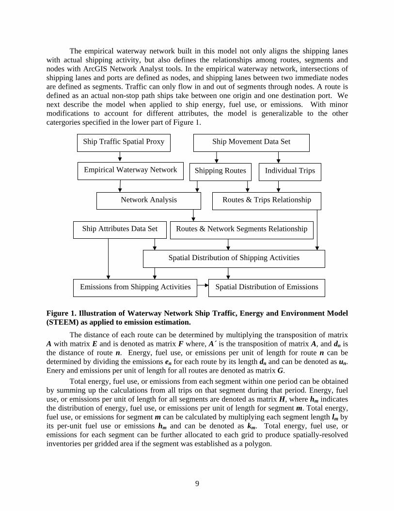
(STEEM) as applied to emission estimation........................................................................... 9 Figure 2. Illustration of spatial distribution of SO2 from North American shipping; shaded areas

represent approximate delineation of coastal exclusive economic zones (EEZs). ............... 19 Figure 3. Comparison of the inventories produced with Waterway Network-STEEM and top-

down approach using ICOADS. ........................................................................................... 22 Figure 4. Illustration of domains of regional/port emission inventories studies........................... 22 Figure 5. Comparison of emissions inventories of different approaches; emissions for Houston &

Galveston are NOx, emissions for the other areas are SO2................................................... 23 Figure 6. Container statistics from U.S. Maritime Administration and American Association of

Port Authorities..................................................................................................................... 25 Figure 7. South Coast (South Pacific) growth rates derived from historic data (1997-2003),

showing upper-bound (exponential), lower-bound (linear), and average trends. ................. 28 Figure 8. US container growth trends from data extrapolation (1997-2003) and from unpublished

draft RTI trade-energy model. .............................................................................................. 28 Figure 9. Model domain showing hypothetical with-SECA region and baseline 2002 model

results. ................................................................................................................................... 30 Figure 10. Illustration of 2020 ship SOx emissions without SECA reductions............................ 31 Figure 11. Illustration of 2020 ship SOx emissions with hypothetical SECA region. ................. 32 Figure 12. Global indices for seaborne trade, ship energy/fuel demand, installed power. ........... 34 Figure 13. Forecast reduction in 2020 of annual SOx emissions due to hypothetical SECA....... 36 Figure 14. Forecast increases from base-year inventory in SOx emitted in 2020 with SECA..... 37 Figure 15. Trends with and without IMO-compliant SECA, and with 0.5% SECA .................... 38 Figure 16. Uncertainty in model output from input parameters scaled by contribution to output

variance. ................................................................................................................................ 40 List of Tables Table ES-1. Baseline 2002 inventory of emissions and fuel use in North American Domain

(metric tonnes)………………………………………………………………………..…vii Table 1. Summary of engine power and at-sea load profile ......................................................... 16 Table 2. Emission Factors............................................................................................................. 17 Table 3. Summary of auxiliary engine SO2 emissions factor ....................................................... 17 Table 4. Baseline 2002 inventory of emissions and fuel use in North American Domain1 ......... 19 Table 5. Estimated Domain Emissions by Vessel Type .............................................................. 20 Table 6. Estimated Percent of Total Emissions from Auxiliary Engines (AEs).......................... 20 Table 7. Power-based growth rate summary for commercial ships 2002 -2020 (CAGR)............ 29 Table A-1. State-by-state Summary of Ports and Port Calls .…………………………………...50 Table A-2. U.S. Port and Waterway Summary from USACE Foreign Commerce Data ...…..…51 Table A-3. Canadian Port and Waterway Summary from LMIU Movement Data …………..…57 Table A-4. Mexican Port and Waterway Summary from LMIU Movement Data .…………..…61

v

ABSTRACT This report presents results of a project to develop and deliver commercial marine

emissions inventories for cargo traffic in shipping lanes serving U.S. continental coastlines. A regional scale methodology consistent with port-based inventory methods was applied for estimating commercial marine vessel (CMV) emissions in coastal waters. Geographically resolved inventories were produced for a 2002 baseline year (Task 1). Several port-based inventories were evaluated to validate the regional inventory (Task 2). Using average growth trends describing trade and energy requirements for North American cargo and passenger vessels, an unconstrained forecast was developed to describe a business as usual (BAU) scenario without sulfur controls (Task 3), and a with-SECA scenario assuming IMO-compliant reductions in fuel sulfur to 1.5% by weight for all activity within the Exclusive Economic Zone (200 nautical miles) of North American nations (Task 4). This work contributes to better regional inventories of commercial marine emissions for North America that supports the California Air Resources Board (ARB), Commission for Environmental Cooperation of North America (CEC), western regional states, United States federal, and multinational efforts to quantify and evaluate potential air pollution impacts from shipping in U.S, Canadian, and Mexican coastal waters.

vi

EXECUTIVE SUMMARY Background: Current best practices for marine vessel emissions inventories have not

been applied to spatially and temporally describe North American interport shipping activity until now. (Interport shipping is ship activity voyaging between ports; it does not include dockside hotelling.) We produced a baseline (2002) emissions inventory for ships engaged in foreign commerce arriving at U.S. ports, and for ship activity in Canada and Mexico by commercial cargo and passenger vessels (excluding ferries). We forecast inventories for business-as-usual (BAU) and for a hypothetical SOx Emission Control Area (SECA) including the Exclusive Economic Zone (EEZ) of North American nations (i.e., 200 nautical miles). The base-year inventory and forecasts assist the California Air Resources Board (ARB) in evaluating air quality and health impacts in California, and help evaluate national impacts, providing part of the required information to request a North American SECA (or SECAs) on behalf of the United States, Canada, and Mexico at the International Maritime Organization (IMO).

Methods: We use a network model, the Waterway Network Ship Traffic, Energy and Environment Model (STEEM), to quantify and geographically represent inter-port vessel traffic and emissions for North America, including the United States, Canada, and Mexico. The model estimates main and auxiliary engine emissions from nearly complete historical North American shipping activities and individual ship attributes, applying activity-based emissions estimates in a GIS platform using an empirically derived network of shipping routes.

We evaluate various sources of growth projections for commercial marine activity and energy use, ultimately choosing an adjusted extrapolation scenario from historic trends in installed power on ships calling on North American ports. Use of installed power trends depends on the following assumptions: 1) commercial marine vessels in cargo service design power systems to satisfy trade route speed and cargo payload requirements; 2) commercial marine vessels operate under duty cycles that are well understood, especially at sea speeds; 3) installed power trends for ships calling on North American ports directly reveals the trend in speed and size for these routes. Trend extrapolations for installed power reveal the correlated trend in energy use by ships, although different extrapolations approaches yield different forecasts. An unconstrained exponential fit may be overly optimistic given economic cycles in shipping and technological change in the fleet; a linear fit may be unrealistic with regard to fundamental work-energy principles and economic drivers for global trade. These define bounding limits for expected change in ship activity. We average these to describe a BAU growth trend that implicitly reflects a mix of positive and negative drivers for ship energy requirements.

Results for Baseline Inventory: North American shipping consumed about 47 million tons of heavy fuel oil and emitted ~2.4 million tons of SO2 in 2002, with approximately 30 million tons fuel and 1.6 million tons SO2 within the North American domain for this project. Comparison of our results with port and regional studies shows good agreement, and improved accuracy over existing top-down methods. Shipping activity within the domain, defined for this project by consensus with the North American SECA team. Table ES-1 summarizes the interport inventory estimates for the baseline year of 2002. The table presents results for coastal regions (defined as the 200 nautical mile EEZ) by nation, and the total for all domain areas outside coastal regions. Comparison of our results with five inventories from other regional and port emissions inventories studies (including Great Lakes, Western Canada, the Port of Los Angeles, Houston & Galveston area, and the Port of New York and New Jersey) showed no bias and better accuracy using STEEM than top-down emissions inventories.

vii

Results for Forecasts: We estimate a growth trend for North America (including United States, Canada, and Mexico) of about 5.9%, compounded. We produce two classes of forecasts: 1) a business as usual (BAU) forecast applying a common growth trend without sulfur controls (but with existing IMO NOx requirements); and 2) a with-SECA scenario assuming IMO-compliant reductions in fuel sulfur to 1.5% by weight for all activity within the Exclusive Economic Zone (200 nautical miles) of North American nations. Our BAU scenario compares reasonably well with available energy and fuel usage trends and with trends describing growth in trade volume; our growth trends are lower than have been reported since 2002 by major US ports. We identify no systemic bias in our forecasts. Various trends agree under BAU scenarios that energy used by ships bringing global trade to and from North America will double by or before 2020. Forecasts show that implementing a North American SECA region reducing fuel-sulfur content from 2.7% to 1.5% (whether through fuel changes or through control technology) will reduce future SOx emissions (as SO2) by more than 700 thousand metric tons (~44%) from what they may otherwise grow to be in 2020. However, our 2020 inventory with an IMO-compliant SECA represents an increase over emissions in the 2002 base-year of more than 2 million metric tons of SOx emissions throughout the North American domain. At a growth rate of 5.9% from the baseline year 2002, trade growth offsets emissions under a 1.5% fuel-sulfur SECA by 2012; using alternative growth rates of 3.6% (separate work presented to the West Coast SECA team), emissions within a North American SECA return to 2002 levels by 2019.

Conclusions: Baseline (2002) inventory results are being used by ARB, the U.S. Environmental Protection Agency (U.S. EPA), Environment Canada, and others to model atmospheric fate and transport of pollution, evaluate air quality impacts, and assess potential health effects attributed to ships. Health and environmental impacts evaluated using these inventories may merit emissions control beyond current IMO standards to maintain emissions targets despite trade growth. Future work could improve precision of near-port inventories through improved network or vessel activity details.

Table ES-1. Baseline 2002 inventory of emissions and fuel use in North American Domain (metric tonnes)1 NOx as NO2 SO2 CO2 HC PM CO Fuel Use United States EEZ2 West Coast 135,000 80,200 4,817,000 4,470 11,300 10,500 1,480,000 East Coast 255,000 151,000 9,095,000 8,440 21,300 19,900 2,800,000 Gulf Coast 174,000 103,000 6,201,000 5,750 14,500 13,600 1,910,000 Great Lakes 16,200 9,620 578,000 540 1,350 1,260 178,000 Alaska 63,300 37,600 2,260,000 2,100 5,300 4,940 697,000 Hawaii 20,500 12,200 732,400 680 1,720 1,600 226,000 Canada EEZ2,3 West Coast 21,900 13,000 781,000 720 1,830 1,700 241,000 East Coast 96,200 57,200 3,440,000 3,190 8,050 7,500 1,060,000 Great Lakes 10,100 5,980 359,000 330 840 800 111,000 Mexico EEZ2 West Coast 99,400 59,100 3,550,000 3,290 8,320 7,800 1,090,000 Gulf Coast 107,000 63,700 3,827,000 3,550 8,970 8,000 1,180,000 Total Coastal regions 998,000 593,000 35,640,000 33,100 83,500 77,900 10,980,000 Non-coastal regions4 1,740,000 1,040,000 62,200,000 57,700 146,000 136,000 19,170,000 Total in Domain 2,740,000 1,630,000 97,800,000 90,800 229,000 214,000 30,160,000

1. Values are rounded to three significant figures for presentation; sums may vary as a result of rounding. 2. National estimates of EEZ boundaries use an ArcGIS buffer of 200 nautical miles and informal national divisions. 3. Western Canada summaries include emissions in the Northwestern part of the domain; Eastern Canada summaries

include emissions in the Northeastern part of the domain. 4. Non-coastal regions are areas in the Domain not within the EEZ of Canada, United States or Mexico.

1

1.0 INTRODUCTION This report is intended to assist the role of the California Air Resources Board (ARB) and

other agencies evaluating the feasibility and extent of a North American Sulfur Emissions Control Area (SECA) as defined by the International Maritime Organization (IMO) in terms of potential impact to air quality and human health by oceangoing commercial marine vessels in transit.

1.1 Purpose and Scope A primary objective of this project is to describe a regional scale methodology for

estimating commercial marine vessel (CMV) emissions in coastal waters (i.e., the Exclusive Economic Zone or EEZ) that is consistent with port-based inventory methods. There are several tasks that follow from this objective, including: Task 1 Provide a baseline inventory of CMV emissions at a regional scale appropriate for modeling

impacts relevant to potential SECA designation. Using this methodology, this work produced a spatially resolved inventory of CMV emissions for North America for a baseline year of 2002. This represents a distance larger than the Exclusive Economic Zone for the continental United States and Canada and Mexico, a legal area beyond and adjacent to the territorial sea that provides certain federal authority to protect and preserve the marine environment (1).

Task 2 Evaluate several port-based inventories in terms of their potential agreement and validation of the regional inventory. We conclude that different assumptions, inputs, or methods applied in port-based inventories produce expected differences reflecting more detailed local information at the port level that cannot be easily reflected at the regional scale. Based on our results, we offer recommendations to improve regional inventory methods or otherwise reconcile differences with port-based inventories.

Task 3 Forecast how baseline emissions may change in future years. Future emissions will be dependent in part upon the changes in emission factors (due to MARPOL Annex VI, other policy, and other changes in engine characteristics), changes in vessel size and number. Additionally, changes may occur in vessel activity patterns and trade routes, and changes in fuel quality (especially sulfur content) – from a mix of technology, economic, and/or policy drivers.

Task 4 Forecast future-year ship emissions under a potential SECA designation. Modification of future-year baseline emissions are made using MARPOL Annex VI requirements that requires the sulfur content of marine fuel used by marine engines within a SECA be equal to or less than 1.5% S by weight. This project supports ARB efforts to understand the significance of ship emissions, by

providing forecasts of CMV emissions under assumptions that describe trade-driven fleet growth, technological changes, and potential designation of special areas under the IMO’s MARPOL Annex VI convention, called SOx Emission Control Areas (SECAs).

1.2 Project Background and Assumptions ARB is participating in a collaborative effort to understand and quantify potential impacts

of CMV activity on North American pollutant emissions, air quality, and public health. This collaboration is led by the U.S. EPA, with agency support also from Environmental Canada, and ARB, and with funded participation by various university researchers and consulting firms. Similarly, the California Goods Movement Action Plan and related efforts to improve freight transportation infrastructure and environmental performance are multi-scale and multi-

2

dimensional interests that depend on a good understanding of international freight movement through major U.S. ports, including but not limited to California ports.

While ARB may be most interested in how CMV emissions and their mitigation may affect California, the international nature of shipping and multi-jurisdictional nature of policy alternatives established a scale of interest that includes all North America. According to the World Shipping Council’s container cargo rankings of U.S. ports (2), the ports of Los Angeles and Long Beach together accounted for more than 36% of all U.S. containerized imports and exports in 2003; together with Oakland, CA ports handle nearly half of all U.S. waterborne containerized cargoes.

This report presents inventory methodology, results, and validation for ships engaged in foreign commerce arriving at U.S. ports, and for ship activity in Canada and Mexico by commercial cargo and passenger vessels (excluding ferries). We produce a spatially-resolved, activity-based inventory of North American shipping activity derived from 172,000 port calls in 2002 to Canada, Mexico, and the United States, employing activity-based methods in a GIS network of empirical shipping routes. We derive emissions forecast trends directly from aggregated installed power of ships calling on North American ports; this is because emissions are directly proportional to engine power and load, which for at-sea conditions is highly correlated with total installed power on commercial ships; this direct proportionality of stack emissions to engine power is implicit in the use of power-based emissions factors in activity-based inventory best practices. We then adjust base-year inventory to estimate emissions from commercial marine vessels for 2010 and 2020. Using observed trends in installed power by cargo and passenger vessels calling on North America, we produce two classes of forecasts: 1) an unconstrained forecast applying a common growth trend to forecast a business as usual (BAU) scenario without sulfur controls; and 2) a with-SECA scenario assuming IMO-compliant reductions in fuel sulfur to 1.5% by weight for all activity within the North American nations.

1.3 Previous Work Air pollutants from marine vessels account for a non-negligible portion of the emissions

inventory and contribute to air quality, human health and climate change issues at local, regional and global levels (3-25). According to the U.S. EPA, heavy duty truck, rail, and water transport together account for more than 25% of U.S. CO2 emissions, about 50% of NOx emissions, and nearly 40% of PM emissions from all mobile sources (26, 27). In Europe, freight modes together generate more than 30% of the transportation sector’s CO2 emissions (28). In California, marine vessel ship emissions are a significant concern with regard to state implementation of federal air quality requirements (http://www.arb.ca.gov/msprog/offroad/marinevess/marinevess.htm), particularly for air districts (21, 29)) and for major ports (http://www.portoflosangeles.org/ and http://www.polb.com/).

Better estimation of current and future emissions inventories, including spatial representation, is needed for atmospheric scientists, pollution modelers, and policy makers to evaluate and mitigate the impacts of ship emissions on the environment and human health. In fact, understanding the nature of commercial marine (e.g., cargo) vessel activity and energy use serves both environmental and goods movement goals for the State of California and the nation. This is particularly true for major ports which represent nodes connecting imported and exported ship cargoes with road and rail freight transportation serving the U.S. and global economies.

3

1.3.1 Inventory Development Although emissions estimates and fuel use are related to the energy used by ships, recent

studies call into question the validity of relying on the statistics of marine fuel sales (4, 30-33). Best practices of estimating emissions from transportation overall, and marine vessel emissions inventories specifically, have focused on activity-based estimation of energy and power demands from fundamental principles (4, 30, 32, 34). These approaches have shown that fuel allocated to international fuel statistics is insufficient to describe total estimated energy demand of international shipping. Even if marine fuel sales statistics were perfect, ships may consume fuel far from where they purchase it. At best, regional statistics provide limited insight into the spatial and temporal characteristics of ship energy consumption.

Principle existing approaches for producing spatially-resolved ship emissions inventories generally can be categorized as either top-down or bottom-up. The fundamental difference between these is that in bottom-up approaches emissions are directly estimated within a spatial context, whereas in top-down approaches emissions are calculated without respect to location at an aggregate level and may later be associated with spatial characteristics. In this work, a mixed approach is developed. First, we associate port arrival-departure data with ship characteristics data to identify more than 170,000 voyages for North America and to allow for activity-based inventory methods of estimating emissions for each voyage. Second, we assign routes to voyage origin-destination pairs using an empirically derived routing network in the Ship Traffic Energy and Environmental Model (STEEM); this is a top-down analytical approach in the sense that we are not directly observing actual voyage routes, but modeling them according to a least-distance algorithm intended to approximate a least-cost voyage. Third, we apply activity-based assumptions about vessel speed, power, energy, and emissions directly within the voyage routing network to produce spatially resolved emissions estimates.

Using a top-down approach, Corbett, et al. produced the first global spatial representation of ship emissions using a shipping traffic intensity proxy derived from the Comprehensive Ocean-Atmosphere Data Set (COADS), a data set of voluntarily reported ocean and atmosphere observations with ship locations (3, 11). They assumed that the reporting ship fleet is representative of the world fleet, spatial distribution of ship reporting frequencies represents the distribution of ship traffic intensity, and emissions are proportional to traffic intensity. Endresen, et al. improved the global spatial representation of ship emissions by using ship size (gross tonnage) weighted reporting frequencies from the Automated Mutual-assistance Vessel Rescue system (AMVER) data set (5). They implicitly assumed that ship energy consumption and emissions are proportional to ship size, which is not true for some types of ships, and they observed that COADS and AMVER lead to highly different regional perturbations (5). Wang, et al. addressed the potential statistical and geographical sampling bias of the International Comprehensive Ocean-Atmosphere Data Set (ICOADS, current version of COADS) and AMVER data sets, the two “best” global ship traffic intensity proxies, and made four advancements to improve the accuracy of the top-down approach using ICOADS as spatial proxy (35): i) trimming over-reporting vessels to mitigate geographic and statistical sampling bias; ii) increasing sample size by using multiple-year ICOADS data; iii) weighting ship observations with installed ship power to reflect emissions variability among different sizes and types of vessels; and iv) smoothing the inventory with GIS tools.

The quality of top-down approaches is limited by the accuracy of global emissions estimates, and inventory precision is limited by the representativeness of spatial proxies.

4

Significant differences exist among the various global ship emission inventories (4, 5, 30, 31). Activity-based energy consumption and emissions in the updated inventory by Corbett and Koehler roughly doubled the results of earlier studies (4). Uncertainty exists in the updated inventory such that the upper bound is about 60% higher than the lower bound (4). Discrepancies among different studies and the range between lower and upper bound of the same study can be explained by the uncertainties of marine engine load factor, time in operation, and fuel consumption rates, which vary by ship type, size, age, fuel type, and market situation (30, 31). Variation in these inputs represents first-order barriers to improving the accuracy of the global ship inventory. Second, since both ICOADS and AMVER data sets rely on voluntary reporting and neither of them is randomly sampled, both of them are statistically and spatially biased (35).

Bottom-up approaches were applied by Lloyd’s register and Entec UK Limited to produce regional ship emissions inventories for the European Monitoring and Evaluation Programme (EMEP) area, the Baltic Sea, and the Mediterranean Sea (17, 24, 25). In this type of approach, ship and route specific emissions are estimated based on historical ship movements, ship attributes, and ship emissions factors. The locations of emissions are determined by the locations of the most probable navigation routes, which are great-circle (i.e., radius) routes between transoceanic origins and destinations, adjusted where prohibited by land, ice, or depth; the Lloyds and Entec work was more regional (not transoceanic) and generally followed straight-line routes. Streets, et al. estimated emissions from international shipping in Asian waters based on commodity flow associated with major sea routes (7, 8).The accuracy of this method, which can be categorized as a bottom-up approach using trade as a proxy for emissions, is limited by the assumed relationships between the volume of trade flow and emissions, which are more closely related to ship installed power, load profile, etc., and by the aggregation of individual voyage routes into major shipping lanes.

Although bottom-up approaches appear more precise than top-down methods, large-scale bottom-up inventories also are uncertain because they must estimate engine workload, ship speed, and most importantly, the speculative locations of the routes which determine the spatial distribution of emissions. Given the large number of ship movements and potentially dynamic shipping routes, the accuracy of regional annual inventories in bottom-up approaches is limited when selected periods within a calendar year studied are extrapolated to represent annual totals (17, 24).

1.3.2 Trends and Forecasting

Trend analyses are useful in describing changes that may have occurred in the past or how changes may occur in the future. While past trends can often be observed without an understanding of underlying causes, they are useful when exploring relationships among correlating histories to evaluate causal drivers or correlated indicators of change. Developing future trends (forecasts) represents an uncertain extrapolation of past observations considering explicit or implicit assumptions about how the trend may be affected by sustained or modified drivers or indicators of change.

Forecasts differ depending on their purposes and scales. Some forecasts look to reveal where timely investment and action at a local scale or by a single firm can produce the most benefit (e.g., profit). Validity of insights is determined by whether recommended actions produce expected outcomes for a given decision, not whether the forecast trend or future value is realized. Other forests are intended to be conservative or aggressive; that is, they intend to be biased to serve the decision makers’ value and tolerance for risk and surprise. This may describe large

5

scale forecasts such as emissions or trade trends. One challenging class of forecasts may be considered “difference” forecasts, where alternative scenarios illustrate how “a path taken” may differ from “a path not taken” rather than to determine which is most probable. These kinds of forecasts are common in policy domains, such as energy, environment, and economics (e.g., IPPC scenarios). Certainly, freight forecasting presents one challenging example, especially at the international or multinational scales, and especially when considering policy actions like a SOx Emissions Control Area (SECA) under IMO MARPOL Annex VI (36).

Previous studies described global growth rates for maritime shipping energy and emissions based on fleet size, trade growth, and/or cargo ton-km, mostly calibrated to linear or conservative extrapolations of historic data. The IMO Study on Greenhouse Gas Emissions from Ships (37) used fleet growth rates based on two market forecast principles, validated by historical seaborne trade patterns: 1) World economic growth will continue; and 2) Demand for shipping services will follow the general economic growth. The IMO study correctly described that growth in demand for shipping services was driven by both increased cargo (tonnage) and increased cargo movements (ton-miles), and considered that these combined factors make extrapolation from historic data difficult. Nonetheless, their forecast for future seaborne trade (combined cargoes in terms of tonnage) was between 1.5% and 3% annually. The IMO study applied these rates of growth in trade to represent growth in energy requirements. The ENTEC study (38) adopted growth rates from the IMO study.

Eyring et al. (39) estimated “future world seaborne trade in terms of volume in million tons for a specific ship traffic scenario in a future year” using a linear fit to historical gross domestic product (GDP) data. Interestingly, this represents one of the only studies to forecast growth in seaborne trade for energy and emissions purposes at rates faster than GDP. The TREMOVE maritime model (40, 41) estimates fuel consumption and emissions trends derived from forecast changes in ship voyage distances (maritime movements in km) and the number of port calls. According to the TREMOVE report, maritime “fleet and vehicle kilometres grow annually by 2.5% for freight and 3.9% for passengers,” while “port callings grew by 8% compared to the previously used input figures.”

For national CMV emissions, U.S. EPA’s 2003 forecast methodology improved the similarity between economic and emissions forecasts from earlier analyses (23, 42-44), although emissions forecasts represent a compound annual growth rate (CAGR) of about 3.4% (range of 2.8% to 3.8%, depending on pollutant). While shipping growth rates accounted for the effect of increased tonnage in a newer fleet, they do not consider the effect of faster speeds – specifically the additional installed power to meet combined size and speed requirements. Correcting for these factors brings the forecasts for international marine activity into closer agreement with trucking growth rates (especially when rail cargo volume increases are considered), and better describes the role of imports growth on the intermodal freight system.

Freight energy use is correlated to increased goods movement, unless substantial energy efficiency improvements are being made within a freight mode (e.g., U.S. rail) or across the logistics supply network. Even assuming that efficiency improvements from economies of scale reduce energy intensity and emissions rather than being directed to larger and faster ships (e.g., containerships), compounding increases in trade volumes outstrip energy conservation efforts unless technological or operational breakthroughs in goods movement emerge. However, except for the Eyring et al. work, these linear extrapolations appear to present growth rates slower than the economy; these linear extrapolations are likely biased underestimates, because shipping and trade activity has grown (and is forecast to grow) faster than the economy. Freight

6

transportation, particularly international cargo movement, is an important and increasing contributor to global and national economic growth, as well as state and regional economic growth in and around major cargo ports. If growth in GDP and trade volumes is compounded as forecast by economic and transportation demand studies, then growth in energy requirements should be non-linear also. The U.S. Bureau of Transportation Statistics (BTS) recently released a report that describes North American freight activity and trends (45). This document reports growth rates for North America above 7.4% for international trade and above 7.2% across all measures of value, and states that:

“Since 1994, the value of freight moved among the three countries has averaged almost 8 percent annual growth in both current and inflation-adjusted terms, compared with about 7-percent growth for U.S. goods trade with all countries (table 1). In 2005, both goods trade and gross domestic product (GDP) grew in inflation-adjusted terms. Except in 2001 and 2002, during the past decade, U.S. trade with Canada and Mexico has increased at a faster rate than U.S. GDP.”

Growth in goods movement by dollar value may be expected to differ from growth in the volume of goods moved, and in the change in activity by the multimodal fleets (ships, trucks, trains, and aircraft) moving cargo. We confirmed that the contribution of international trade is increasing as a proportion of U.S. gross domestic product (GDP) – i.e., freight transportation is growing faster than U.S. GDP (45, 46). Economic activity related to imports and exports together contribute about 22% of recent U.S. GDP in recent years; whereas, goods movement contributed only about 10% of GDP in the 1970s. Moreover, the dominance of containerized cargoes in seaborne trade suggests that truck and containerized shipments may double by 2025 or sooner (47). GDP in the U.S. is growing at ~3.7% CAGR since 1980, and the freight sector is growing at ~6.4% CAGR over the same period (46). This freight-sector growth rate in terms of dollar value is reflected in the observed ~6.3% to 7.2% annual growth rates of “high-value” containerized trade volumes, particularly from Asia (48).

California studies also describe significant growth expected in commercial marine emissions. The recent Clean Air Action Plan for Southern California ports estimates that emissions of NOx and PM from oceangoing vessels will increase at baseline rates between 5.5% and 6% CAGR, respectively, unless measures are taken to reduce emissions (49).1 These growth rates are consistent with trade growth rates, perhaps modified for IMO-compliant NOx reductions in new vessels expected to call on California ports and descriptive of modest improvements in fuel efficiency through fleet modernization and economies of scale. Studies for Southern California (San Pedro Bay) ports agree that growth in cargo volumes equivalent to 6-7% compounding annual growth rates is expected (50-53). However, increased cargo may not produce a corresponding increase in port calls, as some studies interpret (51). Historic data on port calls to San Pedro Bay have shown the number of ship calls remained between 5,000 and 7,000 calls per year since the 1950s (54). Furthermore, proportional relationships between environmental impacts and goods movement trends are reflected in recent port and regional studies of goods transport and economic activity, particularly for California ports (50, 55-57). 1The Clean Air Action Plan shows emissions control measures may offset near-term growth (at least through 2011) if fully implemented.

7

2.0 MATERIALS AND METHODS This section describes principles, methods, and data used to produce baseline inventories

and future emissions inventory scenarios for North America. This project represents one of the first applications of a network model developed to evaluate ship activity characteristics on large regional and global scales using best-practice assumptions and methods comparable to the latest port-based inventories of ship activity. The Ship Traffic Energy and Environmental Model (STEEM) enables emissions inventory analyses that are not scaled from studies of a subset of ports or smaller regions or patched together from separate inventory efforts (58, 59). Starting with a global empirical network of observed shipping lanes, commercial cargo and passenger ship arrivals and departures from all ports in North America are routed along coastal and transoceanic shipping lanes. Vessel engine, speed, and size data for these vessels are applied to estimate emissions from these vessels in both spatial and temporal domains.

In general, materials for this work include the global network developed at the University of Delaware primarily by Dr. Chengfeng Wang (60), vessel activity data for the United States from the U.S. Army Corps of Engineers (61), vessel movement data for Canada and Mexico from Lloyds Maritime Intelligence Unit (LMIU) provided by Environment Canada and the Commission for Environmental Cooperation, respectively (62, 63). Ship characteristics were also obtained from Lloyd’s ship registry data (64). Inventory assumptions and other model inputs were primarily derived from earlier ARB reports and published work by Dr. Corbett (4, 30, 65), modified through discussion with U.S. EPA contractors and review of port-based best practices (34).

Emissions trends are derived from a pluralistic evaluation of historic time series of the above data and forecast studies that together describe: a) growth expected in international goods movement in economic terms (e.g., seaborne trade); and b) correlated trends in energy required to move more goods in service of global trade in terms of ship fleet characteristics (e.g., vessel type and installed power). For cargo activity, we reviewed studies at port, regional, national, and global scales, all of which document strong growth trends and/or forecast similar rates of continued growth (50-53, 66-71). For vessel activity specific to North American ports, we were able to construct detailed trend characteristics information including vessel type, power, size, and speed characteristics for the period between 1997 and 2003; at the global scale, we developed longer time-series trends in ship characteristics by year of build and from related global studies (39, 64).

Three critical questions for understanding freight activity and environmental impacts defined two phases of the project:

1. Baseline Conditions: What are freight energy and activity patterns? 2. Rates of Change: What is forecast trend in energy needed? 3. Patterns of Change: Where is future freight activity located?

While interrelated, these questions may be evaluated with some independence, and were separated into phases combining Tasks 1 and 2 and combining Tasks 3 and 4, described above. The first phase evaluated baseline conditions by applying STEEM, a model that integrates a GIS routing algorithm allocating North American voyage data to empirically derived global ocean routes with activity-based methodology to estimate emissions. The second phase analyses considered rates of change in energy and emissions, demonstrating that installed power was not only a direct input to estimating baseline emissions, but that installed-power trends described

8

rates of change in fleet energy requirement. These phases are described in detail in earlier technical memoranda, and summarized below.

2.1 Baseline Conditions: STEEM description By applying advanced GIS tools and using better data sets, STEEM adopts the strengths

of both top-down and bottom-up approaches and attempts to overcome the weaknesses in each approach and improves ship emissions inventory both mathematically and theoretically. First, the model builds an empirical waterway network based on shipping routes revealed from observed historical ship locations. The spatial allocation approaches the accuracy of a bottom-up approach by assigning routes from a historically accurate network of actual routes, and is more accurate than a top-down approach, which uses biased spatial proxies. Second, as in a bottom-up approach, this model estimates energy use and emissions using complete historical ship movements, ship attributes, and the distances of routes. Best-practices applied to baseline inventories include identification and use of installed power characteristics, current power-based emissions factors, engine load service corrections, and engine operating time (34, 72, 73). STEEM improves baseline emissions inventories for North American shipping in the following ways:

1. STEEM employs an emprical global waterway network derived from 20-year International Comprehensive Ocean-Atmosphere Data Set (ICOADS) data;

2. The model estimates emissions from nearly complete historical North American shipping activities (some 172,000 trips in U.S. Foreign Commerce Entrances and Clearances data set and Lloyds’ Movement data set) and individual ship attributes while a top-down approach estimates emissions based on statistical analysis;

3. The model is constructed using advanced GIS network analyst technology to solve the most probable route for each individual trip on a global scale;2

4. STEEM establishes explicit mathematical relationships among trips, ships, routes, pairs of ports, and segments of the waterway network using a matrix approach;

5. STEEM uses actual lengths of routes, together with service speed of each individual ship, to calculate hours of operation while top-down approaches estimate annual hours of operation based on fleetwide statistics;

6. STEEM follows best practice to estimate emissions based on ship installed power, service speed, and traveling distance for each trip;

7. STEEM assigns emissions based on the locations of solved routes while earlier bottom-up approaches drew straight lines between origins and destinations manually and top-down approaches allocate global emissions based on biased proxies;

8. STEEM captures transit traffic which contributes to local air quality problems in some areas like Santa Barbara, CA, while port-wide inventories have often ignored or been unable to quantify these effects.

Figure 1 illustrates the ship traffic module of STEEM, which can geographically and temporally characterize ship traffic based on an empirical waterway network, historical ship movement data, and ship attributes data set. The lower boxes in Figure 1 illustrate how we applied ship attributes data to produce activity-based, spatially-resolved emissions inventories. 2 A summary of ~400 North American ports and waterways is provided in the Appendix; these ports connect about with ~1,300 foreign ports in the 2002 U.S. Entrances and Clearances data set; about 950 ports are in the 2002 Lloyd’s movement data set, with some overlapping ports among Canada, Mexico, and the United States.

9

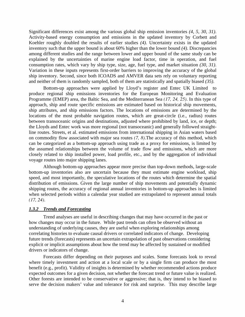
The empirical waterway network built in this model not only aligns the shipping lanes with actual shipping activity, but also defines the relationships among routes, segments and nodes with ArcGIS Network Analyst tools. In the empirical waterway network, intersections of shipping lanes and ports are defined as nodes, and shipping lanes between two immediate nodes are defined as segments. Traffic can only flow in and out of segments through nodes. A route is defined as an actual non-stop path ships take between one origin and one destination port. We next describe the model when applied to ship energy, fuel use, or emissions. With minor modifications to account for different attributes, the model is generalizable to the other catergories specified in the lower part of Figure 1.

Figure 1. Illustration of Waterway Network Ship Traffic, Energy and Environment Model (STEEM) as applied to emission estimation.

The distance of each route can be determined by multiplying the transposition of matrix A with matrix E and is denoted as matrix F where, A´ is the transposition of matrix A, and dn is the distance of route n. Energy, fuel use, or emissions per unit of length for route n can be determined by dividing the emissions en for each route by its length dn and can be denoted as un. Enery and emissions per unit of length for all routes are denoted as matrix G.

Total energy, fuel use, or emissions from each segment within one period can be obtained by summing up the calculations from all trips on that segment during that period. Energy, fuel use, or emissions per unit of length for all segments are denoted as matrix H, where hm indicates the distribution of energy, fuel use, or emissions per unit of length for segment m. Total energy, fuel use, or emissions for segment m can be calculated by multiplying each segment length lm by its per-unit fuel use or emissions hm and can be denoted as km. Total energy, fuel use, or emissions for each segment can be further allocated to each grid to produce spatially-resolved inventories per gridded area if the segment was established as a polygon.

Ship Traffic Spatial Proxy Ship Movement Data Set

Shipping Routes Individual Trips

Ship Attributes Data Set Routes & Network Segments Relationship

Spatial Distribution of Shipping Activities

Network Analysis Routes & Trips Relationship

Emissions from Shipping Activities Spatial Distribution of Emissions

Empirical Waterway Network

10

Matrix A describes the many-to-many relationships across m segments and n routes in the empirical waterway network, where, bm,n is a binary variable that shows whether segment m is part of route n (value of “0” if no, “1” if yes).

nmmmm

n

n

n

bbbb

bbbbbbbbbbbb

A

,3,2,1,

,33,32,31,3

,23,22,21,2

,13,12,11,1

L

MMMMM

L

L

L

= (1)

Relationships between routes and trips can be denoted as matrix B where, tn is the number of trips on route n within one period. The actual number of trips on each route in any temporal period, where trips are defined as a one-way movement on one route, can be derived from ship movement data set, where, tn is the number of trips on route n within one period.

nt

ttt

BM3

2

1

= (2)

Depending on need and data availability, we can either assume ships are identical (as one group or in subsets by vessel type, fuel properties, etc.) or incorporate individual ship characteristics into the model. The number of trips or the indicator of traffic volume weighted by ship attributes on each segment can be denoted as matrix C,where, vm is the number of trips or the indicator of traffic volume of segment m in one period.

mv

vvv

BACM3

2

1

=×= (3)

To estimate fuel use and air emissions out of port areas, we assume ships travel at a typical cruising speed, which appears true in most cases. Fuel use and air emissions from individual trips can be estimated with current best-practice models based on route distance, ship characteristics, and ship operating profile. Total emissions en on route n in one period in which there were tn trips is estimated by equation (4), and fuel use fn can be estimated by equation (5).

),,,,,,(1

Lpamiii

t

inn ellamsdfe

n

∑=

= (4)

),,,,,,(1

Lfamiii

t

inn sfocllamsdff

n

∑=

= (5)

Where, dn is the length of route n, s is vessel speed, m is main engine power, a is auxiliary engine power, lm and la are load factors for main and auxiliary engines, and ep represents emission factor for pollutant p; sfoc in equation (5) represents specific fuel oil

11

consumption (energy rate factor) for fuel type f. Equations (4) and (5) denote that total emissions en or fuel use fn on route n in one period is a function of the length of route, the characteristics of the ships on that route, the operating profile of the ships, and other variables concerned like the quality of fuel, etc. Where vessel-specific estimates are not required, average vessel values can be assigned by vessel type (e.g., tankers, containerized vessels, bulk carriers) to estimate energy, fuel use, or emissions by route.

Energy, fuel use, or emissions from each route can be denoted as matrix D.

ne

eee

DM3

2

1

= (6)

Fuel use and emissions per unit of length are determined by dividing the total emissions on one route by the length of that route, which is the sum of the lengths of all segments of the route. The length of each segment can be obtained by GIS tools and can be detonated as matrix E, where, lm is the length of segment m.

ml

lll

EM3

2

1

= (7)

The distance of each route can be determined by multiplying the transposition of matrix A with matrix E and is denoted as matrix F, where, A´ is the transposition of matrix A, and dn is the distance of route n.

nd

ddd

EAFM3

2

1

' =×= (8)

Energy, fuel use, or emissions per unit of length for route n can be determined by equation (8) and can be denoted as un.

n

nn d

eu = (9)

Enery and emissions per unit of length for all routes are denoted as matrix G.

12

nu

uuu

GM3

2

1

= (10)

Total energy, fuel use, or emissions from each segment within one period can be obtained by summing up the calculations from all trips on that segment during that period. Energy, fuel use, or emissions per unit of length for all segments are denoted as matrix H, where, hm is energy, fuel use, or emissions per unit of length for segment m. hm indicates the distribution of emissions over the waterway network.

mh

hhh

GAHM3

2

1

=×= (11)

Total energy, fuel use, or emissions for segment m can be calculated by equation (12) and can be denoted as km.

mmm hlk ×= (12)

Total energy, fuel use, or emissions for each segment can be further allocated to each grid to produce spatially-resolved inventories per gridded area if the segment was established as a polygon.

2.2 Rates of Change: Installed power as first-order trend indicator for CMV emissions Given that energy used and emissions produced during goods movement increases at a

rate correlated to growth in activity, a number of proxies may be used to estimate inventory growth rates. These include: economic activity (GDP and imports/exports value), trade activity (tons and ton-miles), and fuel usage (sales and estimates). All of these are indirect proxies (second or higher order) of the activity that produces emissions. Except for complete and accurate fuel usage statistics, none directly describe power requirements for shipboard power plants (propulsion and auxiliary engine systems). Best practices for ship emissions inventories typically use power-based (or fuel-based) emissions factors, because of the implicit proportionality between engine load and pollutant emissions – especially for uncontrolled sources (34, 72). Therefore, we derive emissions trends directly from installed power data for cargo ships in the world fleet.

Assumptions we must make to use trends in installed power are rather simple: 1) international vessels in cargo service generally design power systems to satisfy trade route speed and cargo payload requirements; in other words, there is no economic reason to design propulsion systems for containerships, tankers, etc., with more power than their cargo transport operation requires; 2) international vessels operate under duty cycles that are well understood, especially at sea speeds, which for most vessel types utilize the majority of installed power as reflected in best practice methodologies for activity based inventories of energy and emissions from ships; and 3) ships in commercial cargo service on major trade routes reflect the best fit of

13

ship design to service requirements; in other words, the trends revealed in installed power of ships reveals fleet trends in speed and size. With these assumptions, trends in installed power reveal the correlated trend in energy use by ships.

We evaluated installed power data associated with port calls from USACE and Lloyds Registry (for U.S. activity) and from LMIU data (for Canada and Mexico). Where data were missing in the installed power field for some vessels, we used linear regression statistics within each vessel type associating gross registered tonnage (GRT) and rated power to fill data gaps. Over a period from 1997 to 2003, we observed the trend in total ship calls, their collective cargo capacity (tonnage), and aggregate installed power. Observations provided further confirmation that ship calls change over time differently than cargo capacity; we also observed the expected relationship between growth in cargo capacity and installed power. Based on this analysis (performed for major ports in the U.S. and Canada using 1997-2003 data), related evaluation of trends in world fleet propulsion back to 1970, and discussions with the North American SECA team and with ARB, we used installed power trends to develop emissions forecast growth rates. 2.2.1 Evaluating coupled growth in cargo and energy

A variety of curves could be fit to the multi-year installed-power data. We believe that the underlying driver for growth in energy and emissions for CMVs is economic trade, which has and is expected by all accounts to grow at compounding rates. In theoretical terms, if the underlying functional form driving growth is non-linear, we see no justification for fitting a linear growth curve to the available data points. In practical terms, work and energy to move goods by ship are coupled fundamentally unless operational or technological change occurs. Compounding growth in goods movement could not be associated with a linear trend in energy or emissions unless that decoupling is dramatic. Air emissions control in onroad mobile sources provides examples where this has occurred; emissions trends of CO2 and NOx from heavy-duty trucks were decoupled, because regulatory action required new technologies that reduced NOx emissions substantially despite increased energy use over the same period (26, 27).

An important question is whether forecasts that directly apply seaborne trade growth rates to energy and emissions trends should assume any change in the fleet-average energy intensity over time. In international shipping, economies of scale and a shift to thermally efficient slow-speed diesels over the past three-to-five decades have served as the major drivers for technological change; ship air emissions remain the least regulated mobile source, and IMO regulations do not compare with the stringency of onroad standards. A common belief is technological change improves energy efficiency in ocean freight transportation (i.e., reduces energy intensity) over time; rationale for this belief may extend from two historical facts about shipping and energy use: 1) shipping has traditionally been less energy intensive than other freight modes (especially trucking), and 2) marine propulsion engineering developments over the past century produced what are arguably the most fuel-efficient internal combustion (diesel) engines in the world (74).

Our hypothesis was that these conditions may, at best, result in a less aggressive compounding growth in installed power, not a decoupling of work and energy significant enough to justify a linear fit to installed-power data. Depending on change in energy intensity and/or emissions through investments in economies of scale, fuel conservation measures, or emissions control measures, the rate of change in energy and emissions could be a modified growth curve from the growth in cargo activity. If so, one indication would be different rates of change for installed power on ships providing goods movement compared to changes in cargo volume. In

14

other words, if a fleet of ships can carry more cargo without a proportional increase in installed power, then it must be adopting improved technologies (e.g., hull forms, engine combustion systems, plant efficiency) or innovating its cargo operations (e.g., payload utilization).

In fact, the opposite trend is observed in the world fleet over the past 20 to 30 years, where fleet installed power has grown at rates faster than global trade growth. Fleetwide improvements in fuel economy (indicated for marine engines by in-service specific fuel oil consumption averages and/or thermal efficiency) have been much smaller than growth in seaborne trade and CMV installed power. The compound annual growth rate (CAGR) for installed power since 1985 is ~10.7% per year, more than twice the rate of world seaborne trade growth, driven by increases in containership power which grew at more than 16% CAGR over these two decades. While the slope before 1980 appears similar to the slope after 1985, one can observe the significant fleet restructuring (particularly for tankers) during the economic recession in the early 1980s. Choosing a period since 1970 (inclusive of the 1980s shipping recession), the rate of installed power growth for the world fleet ~5.1% CAGR; even so, power growth rates for the liner fleet over this period were still greater than 9% CAGR.

Rephrasing, ocean shipping may have become more energy intensive, not more energy conserving. This seemingly counter-intuitive observation is explainable in terms of globalization and containerization of international trade. Globalization has resulted in longer shipping routes, and containerization serves just-in-time (or at least on-time) liner schedules; both of these drivers motivated economic justification for larger and faster ships which require greater power to perform their service. Increasingly over the past two decades, ships serving all routes became faster and larger through intentional expansion and aging fleet transition from prime routes to secondary markets.

Of course, trends in installed power serving North America may differ from this global installed-power trend. Introduction of the fastest, largest ships first occurs on the most valuable trade routes (e.g., serving North America and Europe) where economics most justify the higher performing freight services. Given this, recent power growth trends for North America could be lower than the global average rate because recapitalization of ships on these mature containerized routes is not so heterogeneous, while larger and faster ships sold on the current second-hand market may have significantly more power than the ships they replace. We observed this to be true. A simple exponential curve fit to installed power produced an initial growth rate estimate of ~7% per year for North America, compared to ~11% globally.

2.3 Patterns of Change: First-order consideration at North American scale This project identified heterogeneity in growth rates among several other dimensions.

Containership growth rates are significantly larger than growth in dry bulk and tanker ships, for both seaborne trade volume and installed power. Energy use and emissions on routes to major containerized ports, therefore grows faster than routes primarily serving bulk trades. Regionally, growth in West Coast ports is generally stronger than North American average growth rates.

While results reveal heterogeneity in CMV growth rates, timing and budget limitations prevented us from forecasting growth rates spatially by vessel-route combination. Maps forecasting emissions applied North American average growth rates to our base-year inventory patterns. By increasing emissions proportionally for all routes on all North American coastlines, our spatially resolved forecasts necessarily underestimate growth on the West Coast where emissions from containerized trade are growing faster than the national average and overestimates emissions growth in regions where overall trade growth is slower, such as the Gulf

15

of Mexico served mostly by bulk ships. As such, this represents a first-order forecast appropriate to consider the value of a SECA for North America but not explicit enough without additional work to apply to other large-scale issues such as port development or regional shifts in traffic.

16

3.0 RESULTS This section describes specific input parameters chosen for STEEM and presents 2002

baseline inventory results required under Task 1; we also summarize Task 2 comparisons and validation using port-based and regional inventories. This section then presents results of BAU forecast trends required in Task 3 using the adjusted power-based extrapolations discussed previously, and a with-SECA scenario under Task 4 that assumes IMO-compliant reductions in fuel sulfur to 1.5% by weight for all activity within the Exclusive Economic Zone (200 nautical miles) of North American nations.

3.1 Baseline Emissions Estimates Main engine power of individual ships was used to estimate ship energy, fuel use, or

emissions for each trip. We adopted the at-sea main engine load factors used by Corbett and Koehler for the updated emissions inventory for international shipping (4). Based on engine manufacturer data used in other global analyses, we assumed that 55% of passenger vessel total main engine power is devoted to propulsion, and 25% of remaining power serves Auxiliary Engine (AE) power (4, 30). We used maneuvering load profile (lower engine load factor and slower ship speed) for the first and last 20 kilometers of each trip when a ship is entering or leaving a port. If the trip was shorter than 20 kilometers, we assumed that ships were maneuvering for the whole trip; although this assumption may underestimate emissions from some short-sea routes. We assumed that main engines operate at 20% of the installed power during maneuvering, the same number used by Entec UK Limited (17).

Since most of auxiliary engine data for ships are missing in the ship attributes data set, average auxiliary power of each ship type was used to estimate the energy, fuel use, or emissions from auxiliary engines. California Air Resources Board (ARB) survey results indicate that "29 percent of the auxiliary engines used marine distillate and 71 percent used HFO, except for passenger vessels that use approximately 8 percent marine distillate and 92 percent HFO" (75). This number was adopted to adjust the SO2 emissions factor for auxiliary engines. Table 1 summarizes the engine power and at-sea load profile used in this work. The average total installed auxiliary engine power was adopted from ARB survey (75); as documented by ARB and others, most vessels have multiple auxiliary engines.

Table 1. Summary of engine power and at-sea load profile Vessel Type Average ME

Power (kW) At-sea ME load (% MCR)

Average Total AE Power (kW)

At-Sea AE Load

Bulk Carrier 7,954 75% 1,169 17% Containership 30,885 80% 5,746 13% General Cargo 9,331 80% 1,777 17% Passenger/Cruise 39,563 55% 39,563 25% Refrigerated Cargo 9,567 80% 1,300 20% Roll On-Roll Off 10,696 80% 2,156 15% Tanker 9,409 75% 1,985 13% Miscellaneous 6,252 70% 1,680 17%

We use emissions factors shown in Table 2. Consistent with previous studies and with

both the ICF report and ARB survey results, we assume all main engines use residual fuel - this is standard practice especially in transit at sea. The emissions factors reported in the recent ARB

17

report “Emissions Estimation Methodology for Ocean-Going Vessels” are nearly identical to those in the ICF best practices paper, and indeed nearly identical to emission factors used in all recent analyses in the U.S., Canada, and Europe (4, 17, 34, 75, 76). We use the composite EF for our work because our data do not explicitly identify by voyage whether the main engine is slow or medium speed or whether the auxiliary engine uses distillate or heavy fuel. This composite may be recalculated for the Great Lakes if data for that region enables more specific analysis of the vessel, engine, and fuel characteristics.

Table 2. Emission Factors Main Engine Emission Factors - In-Transit Operations (g/kWh)

Engine Type Fuel Type NOx SOx CO2 HC PM* CO** Slow Speed Heavy Fuel Oil 18.1 10.5 620 0.6 1.5 1.4 Medium Speed Heavy Fuel Oil 14 11.5 677 0.5 1.5 1.1 Composite EF Heavy Fuel Oil **** 17.9 10.6 622.9 0.6 1.5 1.4

Auxiliary Engine Emission Factors (g/kWh) Engine Type Fuel Type NOx SOx CO2 HC PM CO*** Medium Speed Marine Distillate 13.9 4.3 MDO

1.1 MGO 690 0.4 0.3** 1.1

Heavy Fuel Oil 14.7 12.3 722 0.4 1.5* 1.1 Composite EF **** 14.5 9.1 713 0.4 1.2 1.1

* Emission Factors from ARB Staff ** Emission Factors from Environ Report *** Port of Los Angeles **** Composite used population weighting from ARB OGV Survey, 2005

Considering emissions factors used in previous studies, we used a composite SO2

emissions factor of 10.6 g/kWh to estimate main engine SO2 emissions (4, 17). The SO2 emissions factors for auxiliary engines using marine distillate oil (MDO) and heavy fuel oil are 4.3 g/kWh and 12.3 g/kWh respectively; for this study we do not assume oceangoing ships use marine gas oil (MGO). A composite SO2 emission factor was adopted for each type of ship, weighted by the percent of marine distillate used by that type of vessel (75). Table 3 summarizes the auxiliary engine SO2 emissions factors used for each type of ship in this work. The percent in-use marine distillate of auxiliary engines was adopted from the ARB survey (75). For estimating fuel consumption, 206 g/kWh was used as Specific Fuel Oil Consumption (SFOC) for transport ships and 221 g/kWh for miscellaneous (non-transport) ships, including fishing and factory vessels, research and supply ships, and tugboats, as adopted in other studies (4).

Table 3. Summary of auxiliary engine SO2 emissions factor

Vessel Type Percent In-Use Marine Distillate

Composite Aux. EF (g/kWh)

Bulk Carrier 29% 9.98 Containership 29% 9.98 General Cargo 29% 9.98 Passenger/Cruise 8% 11.66 Reefer 29% 9.98 RORO 29% 9.98 Tanker 29% 9.98 Miscellaneous 100% 4.3

18

We estimated that inter-port transport of North American commerce (including global voyage transits on route segments outside the project domain) consumed more than 44.7 million tons of heavy fuel oil and emitted about 2.3 million tons of SO2 in 2002, about 16.5% of SO2 emissions from all sources in the U.S. in the same year (77). Given that in-port emissions are about 2 to 6% of total emissions, as reported by Streets et al. and Entec UK Limited (8, 17), total heavy fuel use and SO2 emissions from North American shipping are approximately 47 million tons and 2.4 million tons, respectively. The North American shipping fuel use and SO2 emissions are between 18-20% of the world commercial fleet estimated by Corbett and Koehler and between 28-34% of the world cargo and passenger fleet estimated by Endresen et al. (4, 5).

We estimated that ships carrying U.S. foreign commerce consumed about 38 million tons of fuel in 2002 (again including global voyage transits on route segments outside the project domain). This number agrees well with Energy Information Administration statistics that estimate that ships consumed about 44 million tons of fuel in 2002. U.S. domestic waterborne commerce, which we did not include in this work, may be partially responsible for the difference. Moreover, it is likely that the actual distance ships travel often is longer than the distance estimated by the STEEM because data for this work include North American voyages only between prior and next ports and do not model multi-port logistics activity common to commercial shipping (especially containerships).

Containerships, bulk carriers, and tankers account for about 35%, 22%, and 17% of SO2 emissions from North American shipping, respectively. Other types of ships jointly account for the remaining 26%. The top ten maritime countries collectively account for about 71% of the 2.3 million tons of SO2 emissions. Panama, the largest flag of convenience country, accounts for 23% of the SO2 emissions. Liberia, Bahamas, and the U.S. account for 13%, 8%, and 5% of the emissions, respectively. The Norwegian International Register, Singapore, Greece, Cyprus, Malta, and Hong Kong each account for between 3-4% of the emissions. The other 111 countries account for the remaining 29% of the emissions. The energy use profile is similar to the SO2 emissions profile.

3.2 Producing Spatially Resolved Emissions Inventories for Various Pollutants (Task 1) Based on relationships among trips, routes and segments of the network, we allocated

total emissions onto the waterway network. We buffered the network with the width of each segment and calculated the area of the segments in ArcMap. We calculated average emissions per square kilometer by dividing total emissions for each pollutant in each segment with its area. We converted the buffered network to a raster file with a resolution of 4 kilometers by 4 kilometers, where each grid value is emissions from this 16 square kilometer area. We adjusted emissions within a 20-kilometer radius circle of ports to match maneuvering load profiles. Table 4 summarizes interport inventory estimates for 2002 by coastal regions (defined as the 200 nautical mile exclusive economic zone), by nation, and totals for areas outside coastal regions. Figure 2 illustrates the spatial distribution of annual SO2 from North American shipping. Coastal zones resemble the 200 nautical miles Exclusive Economic Zone (EEZ) but national divisions serve illustration purpose only. Monthly and annual pollutant inventories are posted at http://www.ocean.udel.edu/cms/jcorbett/sea/NorthAmericanSTEEM (SOx as sulfur dioxide, NOx as nitrogen dioxide, CO as carbon monoxide, CO2 as carbon dioxide, PM as PM2.5, and HC as total hydrocarbons).

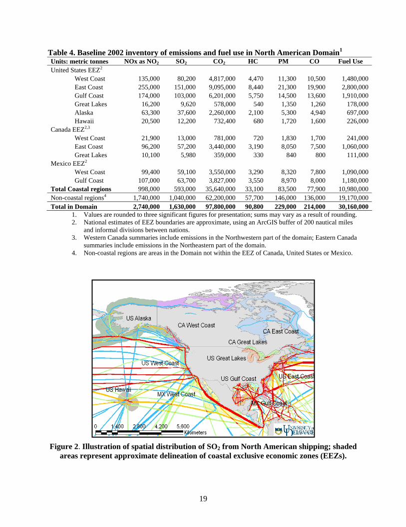
19

Table 4. Baseline 2002 inventory of emissions and fuel use in North American Domain1 Units: metric tonnes NOx as NO2 SO2 CO2 HC PM CO Fuel Use United States EEZ2 West Coast 135,000 80,200 4,817,000 4,470 11,300 10,500 1,480,000 East Coast 255,000 151,000 9,095,000 8,440 21,300 19,900 2,800,000 Gulf Coast 174,000 103,000 6,201,000 5,750 14,500 13,600 1,910,000 Great Lakes 16,200 9,620 578,000 540 1,350 1,260 178,000 Alaska 63,300 37,600 2,260,000 2,100 5,300 4,940 697,000 Hawaii 20,500 12,200 732,400 680 1,720 1,600 226,000 Canada EEZ2,3 West Coast 21,900 13,000 781,000 720 1,830 1,700 241,000 East Coast 96,200 57,200 3,440,000 3,190 8,050 7,500 1,060,000 Great Lakes 10,100 5,980 359,000 330 840 800 111,000 Mexico EEZ2 West Coast 99,400 59,100 3,550,000 3,290 8,320 7,800 1,090,000 Gulf Coast 107,000 63,700 3,827,000 3,550 8,970 8,000 1,180,000 Total Coastal regions 998,000 593,000 35,640,000 33,100 83,500 77,900 10,980,000 Non-coastal regions4 1,740,000 1,040,000 62,200,000 57,700 146,000 136,000 19,170,000 Total in Domain 2,740,000 1,630,000 97,800,000 90,800 229,000 214,000 30,160,000

1. Values are rounded to three significant figures for presentation; sums may vary as a result of rounding. 2. National estimates of EEZ boundaries are approximate, using an ArcGIS buffer of 200 nautical miles

and informal divisions between nations. 3. Western Canada summaries include emissions in the Northwestern part of the domain; Eastern Canada

summaries include emissions in the Northeastern part of the domain. 4. Non-coastal regions are areas in the Domain not within the EEZ of Canada, United States or Mexico.

Figure 2. Illustration of spatial distribution of SO2 from North American shipping; shaded

areas represent approximate delineation of coastal exclusive economic zones (EEZs).

20

3.3 Inventory Summary by Vessel Type While the scope did not require a spatial or temporal representation of emissions by vessel type, the STEEM input data did include vessel-type data. This enabled a post-hoc analysis to estimate emissions contribution by vessel type, as shown in Table 5. This summary represents a proportionally accurate distribution of global routes solved by STEEM, applied to the domain inventory in Table 4. Further work with STEEM to produce maps by ship type would perhaps refine these estimates within the study domain. Table 5. Estimated Domain Emissions by Vessel Type

Ship Type NOx as NO2 SO2 CO2 HC PM CO Fuel Use

Bulk Carrier 610,000 363,000 21,756,000 18,000 45,300 42,300 5,968,000 Container 964,000 574,000 34,413,000 32,300 81,400 76,100 10,723,000 Fishing 1,000 1,000 51,000 20 60 50 7,000 General Cargo 228,000 136,000 8,152,000 7,800 19,800 18,500 2,601,000 Miscellaneous 45,000 27,000 1,605,000 1,600 4,100 3,800 536,000 Passenger 157,000 94,000 5,614,000 5,900 14,800 13,800 1,948,000 Reefer 60,000 36,000 2,150,000 2,300 5,700 5,400 756,000 RO-RO 213,000 127,000 7,607,000 7,100 17,900 16,800 2,362,000 Tanker 461,000 274,000 16,453,000 15,800 39,900 37,300 5,258,000 Total in Domain 2,740,000 1,630,000 97,800,000 91,000 229,000 214,000 30,160,000

These emissions represent both main and auxiliary engines, as discussed above. However, we recognize that the distribution of auxiliary engines differs among vessel types in installed power, fuel type, and emissions. Table 6. Estimated Percent of Total Emissions from Auxiliary Engines (AEs)

Ship Type AE NOx AE SOx AE CO2 AE HC AE PM AE CO AE Fuel Use

Bulk Carrier 2.60% 3.04% 3.70% 2.20% 2.60% 2.50% 3.22% Container 2.40% 2.77% 3.30% 2.00% 2.40% 2.30% 2.93% Fishing 5.00% 2.58% 7.00% 4.20% 5.00% 4.90% 6.13% General Cargo 3.20% 3.67% 4.40% 2.60% 3.10% 3.10% 3.89% Miscellaneous 5.00% 2.58% 7.00% 4.20% 5.00% 4.90% 6.13% Passenger 26.90% 33.33% 34.20% 23.30% 26.70% 26.30% 31.25% Reefer 7.60% 8.76% 10.40% 6.40% 7.50% 7.40% 9.25% Ro-Ro 3.00% 3.44% 4.10% 2.50% 2.90% 2.90% 3.64% Tanker 2.90% 3.33% 4.00% 2.40% 2.80% 2.80% 3.53%

3.4 Comparison with Other Emissions Studies (Task 2) We compared emissions inventories that we produced using a top-down approach with

ICOADS as the spatial proxy with the inventories produced in this work using STEEM (35). In Figure 2, U.S. Coasts are the areas within the 200 nautical mile Exclusive Economic Zone (EEZ) as defined by NOAA in its Office of Coast Survey (78); the Great Lakes include Lake Superior, Lake Michigan, Lake Huron, Lake Erie, Lake Ontario, and connecting waters on both the U.S. and Canadian sides. Figure 3 shows that the emissions calculated with these two approaches agree very well for the US East Coast EEZ but differ to varying degrees on the other two coasts and the Great Lakes (both U.S. and Canadian side).

21

The amount of SO2 emissions within the Gulf Coast EEZ estimated by the network approach is 109% higher than the amount estimated with ICOADS; the amounts by the network approach for the West Coast and the Great Lakes are 32% and 89% lower than the ICOADS approach. The discrepancies between the two inventories can be explained by geographic sampling bias of ICOADS which significantly oversamples the Great Lakes and undersamples the Gulf of Mexico (35).

We also compared our results with the inventories from other regional and port emissions inventories studies (76, 79-82). Figure 4 illustrates the domains of the ports and regions we compared. The Great Lakes include the lakes and connecting waters within the Canadian boundary (76). “Western Canada” represents the coastal areas in British Columbia (B.C.) outside of the Greater Vancouver Regional District (GVRD) and Fraser Valley Regional District (FVRD), and a portion of Washington State, as defined in the Levelton report (82). The Port of Los Angeles, Houston & Galveston area, and the Port of New York and New Jersey (NYNJ) are the areas defined by the Starcrest Consulting Group, LLC in its port-wide air emissions inventory reports (79-81).

Figure 5 shows that the regional/port air emissions inventories produced with different approaches look very different. The emissions inventory produced with the top-down approach using ICOADS as a spatial proxy is significantly higher for the Great Lakes on the Canadian side, but significantly lower for the “Western Canada”, the Port of Los Angeles, and the Port of New York and New Jersey. The conclusion can be drawn that ICOADS is spatially biased as observed in other studies and small-scale emissions inventories produced with ICOADS as spatial proxies may be greatly distorted (5, 35).

Figure 5 also shows that the amount of emissions estimated by STEEM are higher than that of the regional/port studies for the Port of Los Angeles and “Western Canada”, but lower for the Great Lakes on the Canadian side, the port of New York and New Jersey, and the Houston and Galveston area.

We understand that: (1) the STEEM captures transit traffic, which might be ignored in the port-wide studies (Port of Los Angeles and Western Canada) that used arrivals and departures of the specific ports (e.g., the Port of Los Angeles study does not include shipping activity to other San Pedro Bay ports); (2) port-wide studies used more complete arrivals and departure data for the Great Lakes, the Port of New York and New Jersey, and Houston and Galveston; (3) emissions from dockside hotelling are included in the port-wide studies for the Port of New York and New Jersey, and the Houston and Galveston area but are not included in the STEEM results (the portion of hotelling emissions increases and might dominate the emissions inventory when the domain becomes smaller around the terminals and when ships spend less time in transiting); (4) the motivation behind the creation of the STEEM was to improve the emissions inventories from inter-port movements; emissions around ports have to be adjusted by either plugging in the inventories produced by port-wide studies or modifying the model itself to include the dockside emissions; (5) comparisons showing both higher and lower port and reigional estimates suggest there is no systemic error in the STEEM; and (6) our assumption that ships generally maneuver within 20 km (~12.4 miles) of ports may be conservative for many ports, since ARB reports recent Automatic Identification System (AIS) data suggests that ships may operate at sea-speeds until closer to port.

22

0

20,000

40,000

60,000

80,000

100,000

120,000

140,000

US

Gul

fC

oast

US

East

Coa

st

US

Wes

tC

oast

Gre

atLa

kes

tons

of S

O2

emiss

ions

STEEM ICOADS Top-down

Figure 3. Comparison of the inventories produced with Waterway Network-STEEM and top-down approach using ICOADS.

Figure 4. Illustration of domains of regional/port emission inventories studies

23

02,0004,0006,0008,000

10,00012,00014,00016,00018,00020,000

Gre

atLa

kes

(Can

ada)

"Wes

tern

Can

ada"

POLA

NY

NJ

Hou

ston

&G

alve

ston

Met

ric to

ns o

f em

issi

ons

STEEM ICOADS Top-down Port/Regional Inventory

Figure 5. Comparison of emissions inventories of different approaches; emissions for Houston & Galveston are NOx, emissions for the other areas are SO2.

We also observe that the emissions from ships carrying foreign cargo within the 200 nautical miles coastal areas of the United States estimated by the STEEM are about five times of the results estimated by Corbett and Fischbeck using cargo as a proxy (10). We understand that the STEEM is superior to the method used by Corbett and Fischbeck and is more accurate, consistent with the uncertainty discussion in the earlier paper and with the upward correction of more accurate work for the Northwest, United States also published previously (9). 3.5 Forecasting principles

Forecasts can differ depending on their purposes and scales. Some forecasts look to reveal where timely investment and action at a local scale or by a single firm can produce the most benefit (e.g., profit). Validity of insights is determined by whether recommended actions produce expected outcomes for a given decision, not whether the forecast trend or future value is realized. Other forests are intended to be conservative or aggressive; that is, they intend to be biased to serve the decision makers’ value and tolerance for risk and surprise. This may describe large scale forecasts such as emissions or trade trends. One challenging class of forecasts may be considered “difference” forecasts, where alternative scenarios illustrate how “a path taken” may differ from “a path not taken” rather than to determine which is most probable. These kinds of forecasts are common in policy domains, such as energy, environment, and economics (e.g., IPPC scenarios). Certainly, freight forecasting presents one challenging example, especially at the international or multinational scales, and especially when considering policy actions like a SOx Emissions Control Area (SECA) under IMO MARPOL Annex VI (36).

Admittedly, the quality of forecasts of maritime shipping and trade is limited (83), and thus forecasting of environmental impact from shipping is constrained by the quality of shipping and trade forecasts. Therefore, we employed a comparison of historic trends and forecast

24

indicators related to maritime trade and energy to provide reasonable insight into a range of feasible forecasts. Individually, none of these forecasts can be considered more correct than another, as they represent different assumptions about the relationship between transportation energy, trade, and North American port activity. However, taken together, they reveal a bounded range of trends with common insights useful in comparing sulfur controls with no action. We look for converging growth trends that are representative at several scales (port, region, coastal, and national) and informed by historic data. These lead to a set of principles for describing how freight transport emissions may change:

1. Define the forecast domain broadly through multiple perspectives on freight and economy. 2. Compare global, large regional forecasts with local efforts for converging insights, perhaps

allowing for probabilistic assessment. 3. Include the rear-view mirror in forecasting (i.e., compare with persistence). 4. Consider first principles involving energy and environment: Some work-energy relationship

must hold if fuel price matters to freight. 5. Make extrapolation adjustments as simple as possible, but no simpler: Assumptions inter-

relating energy, economy, and technology should be checked for potential inconsistencies. 6. Look for surprise, avoid overconfidence: Recognize heterogeneity at all scales; use detailed

scenarios to help broaden or delineate the forecast range, but do not rely on them as likely.

3.6 Activity-based modeling of freight growth Seaborne cargo activity has increased at significant rates over time. World seaborne

trade growth has increased monotonically except for a short period in the early 1980s (66-69). Containerized trade is growing faster than global rates. Figure 6 illustrates recent containerized cargo trends and TEU throughput since 1980. U.S. Maritime Administration (MARAD) statistics include cargo on both government and non-government shipments by vessels into and out of U.S. foreign trade zones, the 50 states, District of Columbia, and Puerto Rico, excluding postal and military shipments; AAPA statistics describe total container throughput, including empty container movements. Containerized cargo throughput (including empty container movements) grew at ~6.5% CAGR since 1985, with imported cargo grow since 1997 at more than 10% CAGR and total cargo TEUs (excluding empty container movements) growing at ~7% CAGR since 1997. Given the high-value nature of containerized cargoes, it is not surprising that these growth trends are most similar to growth in the value of cargo moved, reported by BTS.

Conceptually, growth in seaborne cargo movement should influence (if not determine) activity growth in the freight modes (truck and rail) carrying imports and exports to or from U.S. metropolitan regions and inland regions. For example, if growth in rail and truck modes is primarily a result of increasing imports, observed in the U.S. to range between 4.6% and 4.8% CAGR for all cargoes and between 6% and 9% for containerized (intermodal) cargoes (~6.5% CAGR for total container throughput including empty containers), then combining these modes should reflect seaborne trade growth rates (71, 84). The multimodal transportation of empty containers presents a unique challenge in understanding how international goods movement affects landside freight modes (85). Moreover, trucking and rail movements include exported and domestic freight movements, which are growing at much lower rates than containerized imports, effectively dampening national growth rates in intermodal freight transportation compared to port throughput. Considering these activities together helps provide an intuitively consistent explanation reconciling steeper seaborne trade trends reported in major ports, and obtained or derived from economic and trade analyses, with less-steep truck and rail freight

25

trends. In other words, we should expect growth rates in goods movement to be shared among modes because freight transportation is an intermodal network of imports, exports, empty repositioning, and domestic freight flows.3

0

5

10

15

20

25

30

35

40

45

1980 1985 1990 1995 2000 2005

Mill

ion

TEU

s

TEU throughput Total Cargo TEUs Export TEUs Import TEUs

Figure 6. Container statistics from U.S. Maritime Administration and American Association of Port Authorities (70, 71).

The U.S. Department of Transportation launched two of the first federal efforts to consider together multimodal and intermodal freight effects of imported cargoes, generally through its “Assessment of the U.S. Marine Transportation System and spatially through the Freight Analysis Framework (FAF) (86, 87). This work produced a forecast of freight transportation activity based on trade increases, primarily to identify infrastructure needs rather than estimate energy and environmental impacts. According to the Freight Analysis Framework (87),4 domestic freight volumes will grow by more than 65 percent from 1998 levels by the year 2020, increasing from 13.5 billion tons (in 1998) to 22.5 billion tons (in 2020). This represents a ~2.3% compound annual growth rate (CAGR), similar to that obtained from VMT growth rates (not adjusted for sales growth) in MOVES (88). In other reports, truck freight has doubled since 1980 (an average annual increase of 3.7%), while domestic waterborne freight has declined by nearly 30% (an average annual decline of 1.8%) (89).5 These rates represent the lowest growth trends we could find in the literature for goods movement.

3 This background discussion does not necessarily imply a direct relationship between energy and emission growth rates and seaborne trade growth rates; depending on efficiency gains and economies of scale (e.g., shown for the rail sector), the rate of change in energy and emissions for ships could be different. This background reinforces the purpose of and need for the forecasts analysis presented in this report. 4 See Freight Analysis Framework documents at http://ops.fhwa.dot.gov/freight/freight_analysis/faf/. 5 BTS Pocket Guide to Transportation 2003, http://www.bts.gov/publications/pocket_guide_to_transportation/2003/.

26

Currently, growth factors embedded in U.S. mobile source energy and emissions models appear to capture better this economic-driven growth in freight transportation. Growth factors for trucking (single-unit and combination trucks) in the U.S. EPA’s mobile source models include a combination of a population (sales) and VMT growth factors, with adjustments for fuel economy and other operational factors (88). U.S. EPA compared rail freight ton-miles with railroad distillate fuel consumption data to indicate substantial improvements in rail freight energy intensity, adjusting emissions based on regulatory requirements (90). And, in its 2003 rulemaking, U.S. EPA assumed that freight growth was linked to increased tonnage volume (23).

Historic and future growth rates for particular modes are consistent with coupled growth in economic-energy-emissions trends. For example, U.S. EPA projects that truck population and VMT will increase by 4.2% to 4.8% CAGR between 2002 and 2025 (88). For rail, U.S. EPA showed that growth rates in cargo ton-miles transported nearly doubled in recent periods, from ~2.4% CAGR between 1980 and 1995 to ~4.8% CAGR between 1990 and 1995 (illustrated in Figure 1-1 in U.S. EPA’s regulatory support document). In fact, updating observed growth rates in cargo ton-miles moved by rail to include more recent years reveal a rail-cargo growth rate of ~3.6% CAGR from 1985 to 2004 (91, 92). 3.5.1 Growth Rates

Most forecasts essentially take historic trends for some recent period and extrapolate with adjustment for expected change in trends (e.g., response to economic and population drivers affecting global trade or consumption). In coming decades, a number of events could modify an unconstrained growth trend in energy use. In terms of technology, there could be further improvements in thermal efficiency, fuel type and quality, and propulsion design. In terms of the economy, we expect shipping cycles to continue to provide periods of slower or negative growth in oceangoing goods movement (83). In terms of logistics operations, trends in containerization economies of scale and vessel speed over the past three decades could change over the next three decades if global inventory, energy, and labor costs change.

A simple exponential curve fit to installed power produced an initial growth rate estimate of 7.1% per year for North America, before averaging with a linear extrapolation. While we recognized the need for similar adjustment in our forecasts, we hesitated to arbitrarily insert “inflection points” in out-year forecasts corresponding to optimistic or pessimistic assumptions. We acknowledge that an unconstrained exponential curve fit would likely overestimate future emissions, particularly given expected shipping cycles; we also observed that a linear growth rate did not match known or expected technology changes relative to cargo growth. A linear trend in energy use would imply less power required to achieve the cargo throughput – where cargo volumes are projected to see compounded growth. We don't believe that average technology in the fleet will change that much from its current path over the next 35 years without strong policy incentive or substantial changes in fleet energy pricing and supply. Overall, fleet propulsion technologies will remain more similar than different to the current profile at least through 2040. Moving more cargo will require more power, in a similar manner to the current fleet (either through larger ships, faster ships, more ships, or some combination). Moreover, we did not identify physical capacity limits to ports or shipping routes (that are not being addressed through infrastructure investment) which would constrain trade growth.

Through discussions with ARB, we agreed that the unconstrained exponential trend and the linear trend define bounding limits for expected change in ship activity. Averaging these curves defines an arbitrary middle-growth trend, which implicitly describes a mix of positive and

27

negative drivers for ship energy requirements without articulating a detailed scenario of conditional events. After adjustment, we estimate a growth trend for North America (including United States, Canada, and Mexico) of about 5.9%, compounded.

Studies for Southern California (San Pedro Bay) ports supported this adjustment. These studies agree that growth in cargo volumes equivalent to 6-7% compounding annual growth rates is expected (50-53).6 Some studies articulate different pathways of growth than simple extrapolation; for example, the no-net-increase (NNI) forecast produces nearly the same result for 2020, but describes substantial increases in the near-term as a result of planned investment in the ports (50). In Figure 7, we show bounding curves (exponential and linear) and the average growth curve for Southern California ports. We converted growth trends from the no-net-increase study and from an unpublished trade-energy model (by RTI under U.S. EPA direction) to describe change in installed power and plotted them in Figure 7 with our extrapolation (50, 93).7

These comparisons demonstrate that increasing cargo throughput is related to technology innovation (e.g., larger ship sizes, higher speeds, and containerization) that promotes economies of scale with more powerful ships, more so than increased cargoes determine the number of voyages. Independent derivations of growth trends all describe at least a doubling of commercial marine energy use and emissions in California by 2020, corresponding to similar change in the expected port cargo throughput.

Agreement between the draft trade-energy model by RTI and extrapolation of observed data is even stronger for containerships. As shown in Figure 8, preliminary results from the draft RTI trade-energy forecast are more aggressive than our power-based extrapolation. RTI’s trade-energy model exception to calibrate on inbound containerized cargoes (“heavy-leg” activity) may explain this (93). Note excellent agreement in RTI draft model results with observed power-trend history for containership calls to U.S. ports. These sources of growth trends and forecasts are consistent with and validate our observed trends in installed power and support our extrapolation of power-based trends to forecast emissions under business-as-usual (BAU) conditions. Using our adjusted extrapolation to forecast growth at ~5.9%, we observe that power-based growth rates derived here are comparable to growth rates for land-based freight modes, by about 1% to 2% (45-48, 71, 84, 88, 91, 92, 94).8 This comparison is expected due to the fact that trucking and rail are also engaged in domestic and intra-continental trade with Canada and Mexico that would not require commercial shipping. Moreover, our forecast rates are generally lower than dollar-value growth in North American seaborne trade, and a bit lower than growth in containerized cargo volume. Again, such comparisons are expected given the importance of bulk cargoes (liquid and dry) to North American international trade. In addition, the lower growth in power-based rates compared to cargo activity provide confirming evidence that economies of scale are improving the energy intensity and emissions intensity of international shipping – but perhaps by not more than 1% to 2% overall yet. Additional analysis by vessel type could quantify these improvements in more detail, perhaps discerning relative roles of speed, size, and operational factors (e.g., average 6 Other studies interpret strong growth in cargo volume to produce a corresponding increase in port calls (51, 54). 7 While RTI work is in draft form, U.S. EPA and ARB coordinated discussions and comparisons between this project and the RTI project. NNI shows only the Southern California ports of Los Angeles and Long Beach, while the RTI work describes the “South Pacific” ports, which are considered to be mainly LA and LB but could include Oakland. 8 Multimodal comparisons are discussed in more detail in Technical Memorandum for Tasks 3-4.

28

payload utilization rate). Lastly, we observe emissions and energy use by the fastest, most powerful ships (containerships) are increasing at the fastest rates, along with demand for containerized trade.

0

200

400

600

800

1000

1200

1990 1995 2000 2005 2010 2015 2020 2025 2030

Fore

cast

ed T

rans

port

Ene

rgy

(kW

)

Unconstrained 7-point Trend

Baseline NNI

This Work

Linear Trend

RTI US South Pacific

Figure 7. South Coast (South Pacific) growth rates derived from historic data (1997-2003), showing upper-bound (exponential), lower-bound (linear), and average trends. Also shown

are trends from NNI Task Force and from unpublished draft RTI trade-energy model.

0

200

400

600

800

1000

1200

1400

1600

1990 1995 2000 2005 2010 2015 2020 2025 2030

Inst

alle

d Po

wer

Est

imat

e

AverageObserved Container PowerRTI Container

Figure 8. US container growth trends from data extrapolation (1997-2003) and from unpublished draft RTI trade-energy model.

29

Table 7 presents an overview of power-based growth rates for selected ports and North American regions. Growth rates for North America, US, Mexico, and Canada use regression statistics within each vessel type associating gross registered tonnage (GRT) and rated power to fill data gaps. General similarity is observed across all regions, with Canada installed-power data presenting the highest rate of growth and with Mexico presenting the lowest rate of growth. These growth rates represent an average of unconstrained exponential curve-fits with linear extrapolation of the data, which implicitly describes an implicit mix of positive and negative growth drivers. Given that such adjustments may not equally influence growth at different ports or regions, it is possible that actual growth in emissions will be higher for some places (and perhaps lower for others), depending on events that modify unconstrained growth trends over the next decades.

Table 7. Power-based growth rate summary for commercial ships 2002 -2020 (CAGR)

Ports, or Region Emissions Growth Rate Los Angeles/Long Beach 5.24% Oakland/San Francisco 5.68% New York/New Jersey 6.03% California (all ports) 5.53%

U.S. West Coast 5.93% U.S. National 5.86%

Canada 6.57% Mexico 5.06%

North America (U.S., Canada and Mexico) 5.86% 1. Growth rates represent an average of exponential and linear fit extrapolations,

presented in terms of compound annual growth rate (CAGR). 2. US data are from USACE and Lloyds Registry data, per this and other work by

Wang and Corbett. 3. Canada and Mexico data are from Lloyds Movement data (LMIU)

3.5.2 Growth Patterns We produced a set of baseline (Tasks 1 and 2) emissions estimates and forecast estimates

(this work, Tasks 3 and 4) conforming to a consensus domain and resolution appropriate for most of the atmospheric modeling that will use our North American ship emissions inventory. This consensus resulted from several meetings with the SECA team. Annual emissions are resolved into twelve monthly components, following time-resolved patterns in ship activity in North America, as discussed in the report for Tasks 1 and 2. The North American inventory estimates for each pollutant uses the following projection parameters from ESRI’s ArcGIS software:

Projection: Equidistant_Cylindrical Parameters: False Easting: 0.0 – default ESRI parameter False Northing: 0.0 – default ESRI parameter Central Meridian: 180.0 degrees – UD defined Standard Parallel_1: 0.0 – default ESRI parameter Linear Unit: User Defined Unit (1000 m) – UD defined Cell Units: kilograms per 16 square kilometers

We delivered inventory files using the following domain:

left -1000 km, right 18000 km, top 8000 km, bottom 0 km.

30

A hypothetical SECA region conforming to the Exclusive Economic Zone (EEZ) for North America was defined for the with-SECA scenarios. Figure 9 shows the model domain and also reproduces the SOx inventory illustration for the base-year 2002. The scale shown for emissions is delineated using units common to forecast inventory illustrations discussed below.

Figure 9. Model domain showing hypothetical with-SECA region and baseline 2002 model results.

3.7 Future Emissions without SECA region (Task 3) Based on trend comparisons discussed above, we use the following ratios for SOx

forecasts: For 2010, we multiply the 2002 base year inventory by 1.61 times; for 2020, we multiply the 2002 base year inventory by 2.79 times, corresponding to a growth rate of 5.9% compounded annually.

For NOx emissions we make adjustment for the introduction of IMO-compliant engines into the international cargo fleet. We use industry data to estimate ~11% percent average reductions in NOx for new engines complying with MARPOL Annex VI (95). This estimated reduction is similar but slightly lower than assigned in other analyses of IMO-compliant NOx reductions (42, 44); further study into the NOx reduction from uncontrolled to IMO-compliant engines is ongoing and may produce better per-engine reduction estimates. Introduction rates for new engines into the fleet are based on fleet scrapping and new ship orders used in previous work (3, 96). Following standard assumptions for the introduction of new engines in the fleet used of 2% per year, we estimate that about 46% of the fleet in 2010 and about 78% of the fleet in 2020 will be IMO-compliant. This accounts for fleet-weighted NOx reductions of 5% and 8.4% in 2010 and 2020, respectively, resulting in NOx multiplier ratios of 1.53 for 2010 and 2.55 for 2020.

Per project scope, we considered whether fuel-sulfur content may change in coming years, e.g., would refining practices result in generally higher fuel-sulfur averages over time as distillate fuels (particularly diesel) removed more sulfur. We chose not to make any adjustments to the average fuel-sulfur content in this work for two reasons. First, we observe very little change in world-average fuel-sulfur content for residual fuels over the past decade; in fact, most of the differences may be attributed to better statistical tracking on behalf of MARPOL Annex VI, more so than real changes in the global average. Second, we recognize that variation in fuel-suflur content regionally may be greater than the average change over time; we understand that U.S. EPA is sponsoring study of this issue, and that results of that work are not yet available. If

31

such trends are proven, they can be implemented at the regional level using STEEM in future work.

An illustration of 2020 emissions without applying any SECA reductions is presented in Figure 10. Annual and monthly data files for 2010 and 2020 for all forecasted pollutants (SOx as SO2, NOx as NO2, CO2, PM, CO, and HC) are provided in both raster and ASCII formats at the project website (http://coast.cms.udel.edu/NorthAmericanSTEEM/).

Figure 10. Illustration of 2020 ship SOx emissions without SECA reductions.

3.8 Future Emissions with Potential SECA (Task 4) To produce with-SECA forecast scenarios, uncontrolled inventories for 2010 and 2020

are modified to depict a reduction in average fuel-sulfur content from 2.7% to 1.5%, a SOx emissions reduction of about 44%. Only SOx emissions are assumed to change under this SECA scenario; no additional reductions in primary PM, NOx or other pollutants are calculated. Within GIS, we select the emissions within the hypothetical SECA region and multiply them by 66% (1 minus 44%). Similar to the forecast without SECA, this makes no assumptions for changes in fuel quality or supply between now and 2020. Such changes could occur through regulatory action in addition to an IMO-compliant SECA, or through a combination of fuel supply and price effects not considered in this work. Such considerations could be included in updated forecasts, based on insights from further (ongoing) studies. Figure 11 illustrates annual SOx emissions in 2020 depicting compliance with the hypothetical SECA domain.

An illustration of 2020 emissions with SECA reductions is presented in Figure 11. Annual and monthly files for 2010 and 2020 for SECA-compliant SOx emissions can be found in both raster and ASCII formats at (http://coast.cms.udel.edu/NorthAmericanSTEEM/). It is worth noting that sulfur inventories represent stack emissions of gaseous sulfur dioxide (SO2), not aerosol sulfate. Ours is a stack emissions inventory, before total fate and transport impacts. It is inappropriate to pre-process gaseous emissions from the stack within an inventory using

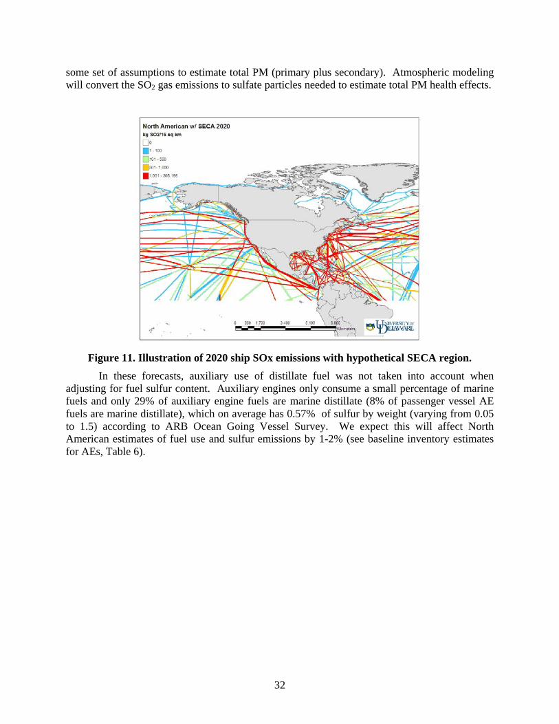
32

some set of assumptions to estimate total PM (primary plus secondary). Atmospheric modeling will convert the SO2 gas emissions to sulfate particles needed to estimate total PM health effects.

Figure 11. Illustration of 2020 ship SOx emissions with hypothetical SECA region.

In these forecasts, auxiliary use of distillate fuel was not taken into account when adjusting for fuel sulfur content. Auxiliary engines only consume a small percentage of marine fuels and only 29% of auxiliary engine fuels are marine distillate (8% of passenger vessel AE fuels are marine distillate), which on average has 0.57% of sulfur by weight (varying from 0.05 to 1.5) according to ARB Ocean Going Vessel Survey. We expect this will affect North American estimates of fuel use and sulfur emissions by 1-2% (see baseline inventory estimates for AEs, Table 6).

33

4.0 DISCUSSION

4.1 Comparison with global forecast trends For validation, we considered whether analyses at a global scale might yield similar

results. We compared world fleet trends in installed power (derived from average power by year of build) with energy trends (Eyring work and fuel sales), with trade-based historical data (tons and ton-miles). Activity-based energy results for similar base-years (2001 or 2002) are within close agreement (72, 97, 98).9 This allows us to index trends to nearly the same value and year, to index trade-based trends similarly, and to compare these with trends in installed power, as summarized in Figure 12. Three insights emerge from this global comparison.

1) Extrapolating past data (with adjustments) produces a range of BAU trends that is bounded and reveals convergence around a set of similar trends; in other words, while the range of growth may vary within bounds of a factor of two, one cannot get “any forecast they want” out of the data. If we consider that global trade and technology drivers mutually influence future trends, then we may interpret convergence within the bounds as describing a likely forecast of global shipping activity.

2) World shipping activity and energy use are on track to double from 2002 by about 2030 (~2015 if one considers seaborne trade since 1985, ~2050 if one considers Eyring’s BAU trend).10 Growth rates are not likely to be reduced without significant changes in freight transportation behavior and/or changes in shipboard technology.

3) Confirming earlier discussion, trends in installed power are clearly coupled with trends in trade and energy. This reinforces the analysis of installed power as a proxy for forecasting growth, not only for use in baseline inventory estimates.

Coincidentally, averaging bounding extrapolations yields between 3.8% and 4.5% CAGR growth in installed power, nearly the same 4.1% CAGR as observed for past world seaborne trade (66, 67, 69). In other words, this explains and confirms the use of seaborne trade growth to project ship fuel use and emissions, as other studies have done. Therefore, we consider this BAU forecast to be informed by observed past trends and consistent with adjustments intended to avoid overly aggressive growth estimates. Consistent with the market-forecast principles reflected in the IMO study, and given the strong relationship observed between cargo moved (work done) and maritime emissions (fuel energy used), we estimate that global emissions from CMVs are increasing at average growth rate of at least 4.1%. This suggests that the rate of growth in emissions for North America is greater than the global average growth rate.

4.2 Uncertainty and Bounding There are six types of uncertainty that affect these results. Three primary sources of

uncertainty involving parameters directly used in this study include a) uncertainty in the base-year estimates; b) uncertainty in the trend used to produce the forecasted inventories; and c) uncertainty in the patterns of future ship traffic. Additionally, uncertainty arises from factors not addressed in this work to date – but that could improve future efforts using these methods. Additional detail could be incorporated to describe better underlying drivers of change in freight

9 An exception is work by Endresen et al, that tends to adjust parameters to agree with international marine fuel sales statistics; their results are within uncertainty ranges described in other work (5, 94, 99). 10 A review of forecast trends for global marine fuel use in unpublished draft results from RTI work suggests that the trade-energy model developed in parallel with this project falls within these ranges.

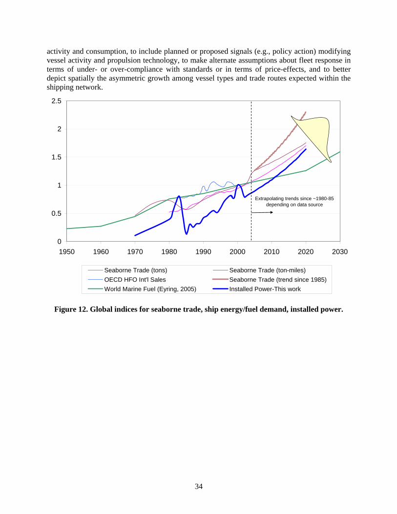
34

activity and consumption, to include planned or proposed signals (e.g., policy action) modifying vessel activity and propulsion technology, to make alternate assumptions about fleet response in terms of under- or over-compliance with standards or in terms of price-effects, and to better depict spatially the asymmetric growth among vessel types and trade routes expected within the shipping network.

0

0.5

1

1.5

2

2.5

1950 1960 1970 1980 1990 2000 2010 2020 2030

Seaborne Trade (tons) Seaborne Trade (ton-miles)OECD HFO Int'l Sales Seaborne Trade (trend since 1985)World Marine Fuel (Eyring, 2005) Installed Power-This work

Extrapolating trends since ~1980-85 depending on data source

Figure 12. Global indices for seaborne trade, ship energy/fuel demand, installed power.

35

5.0 SUMMARY AND CONCLUSIONS

5.1 Baseline Inventory The 2002 inventory of emissions from North American shipping successfully applies

bottom-up estimation methods, extending best-practices for commercial marine inventories to the largest spatially resolved scale so far, and the STEEM model is capable of conducting similar analyses for other regions and even globally. STEEM achieves many of the goals of nonroad marine modeling efforts, such as the U.S. EPA Mobile Vehicle Emissions Simulator (MOVES).11 STEEM exceeds MOVES current design in two important ways: 1) our approach produces spatial and temporal assignment of emissions in GIS; and 2) our model considers individual vessel movements, rather than binning vessels of similar type. (Similar to binning by MOVES, our model applies emissions factor and engine activity assumptions by vessel type, but considers installed power, routing, and speed individually.)

Our results for U.S. EEZ regions in the North American interport shipping inventory can be compared to US domestic freight overall, and compared to US domestic marine statistics (26, 27). For carbon dioxide, our results in U.S. EEZ regions are 32% of CO2 estimate by U.S. EPA for all shipping (coastal and inland ships and boats plus bunkers) and 85% of bunkers only; our estimates represent 6% of CO2 for U.S. surface freight transportation. Our estimates of CO2 emissions and fuel use conform generally to the expected ratio implicit in the fuel-based CO2 emissions factors, around 3200 tons of CO2 per 1000 tons fuel, suggesting the bunker fuel comparison with U.S. EPA is most appropriate for cargo ship activity addressed in this study. The comparison of our work with international bunkers is very good agreement, given the independent analysis and considering that we do not account for bunkers used in port or for fuel used on voyages in addition to transits from prior port or to next port. For NOx, our estimates are 70% of 2002 U.S. EPA NOx estimates from shipping, and represent approximately 12% of NOx from all U.S. surface freight modes (heavy-duty diesel truck, locomotive, and marine including bunkers). For SO2, our estimates in U.S. EEZ regions are 2.5 times greater than estimated by U.S. EPA for shipping, and 1.2 times greater than SO2 from U.S. surface freight transportation. For PM2.5, our inventory estimates in U.S. EEZ regions are 1.4 times greater than current estimates for US shipping, and 34% of U.S. surface freight transportation.

It is important to recognize that at least parts of our inventory may represent shipping not included in these national inventories, and that our inventory does not include some marine activity included in these comparison statistics. For example, we do not include inland river navigation12, and our data does include Canadian and Mexican vessel activity that may transit within U.S. coastal regions. In this regard, the emissions estimated in this work both augment and complement current national inventories. Therefore, further work would be required to evaluate the degree that our inventory may increase existing estimates; therefore, the percentages resulting from this comparison represent a first-order comparison.

11 See http://www.epa.gov/otaq/ngm.htm for MOVES information. 12 Inland river navigation refers to voyages entirely within inland river regions, typically not navigable by deep-draft or oceangoing vessels. River transits by deepwater vessels in bays and deepwater river channels are included in this study (e.g., in San Francisco Bay to Benicia or Redwood City, or in the Columbia River to the Port of Portland).

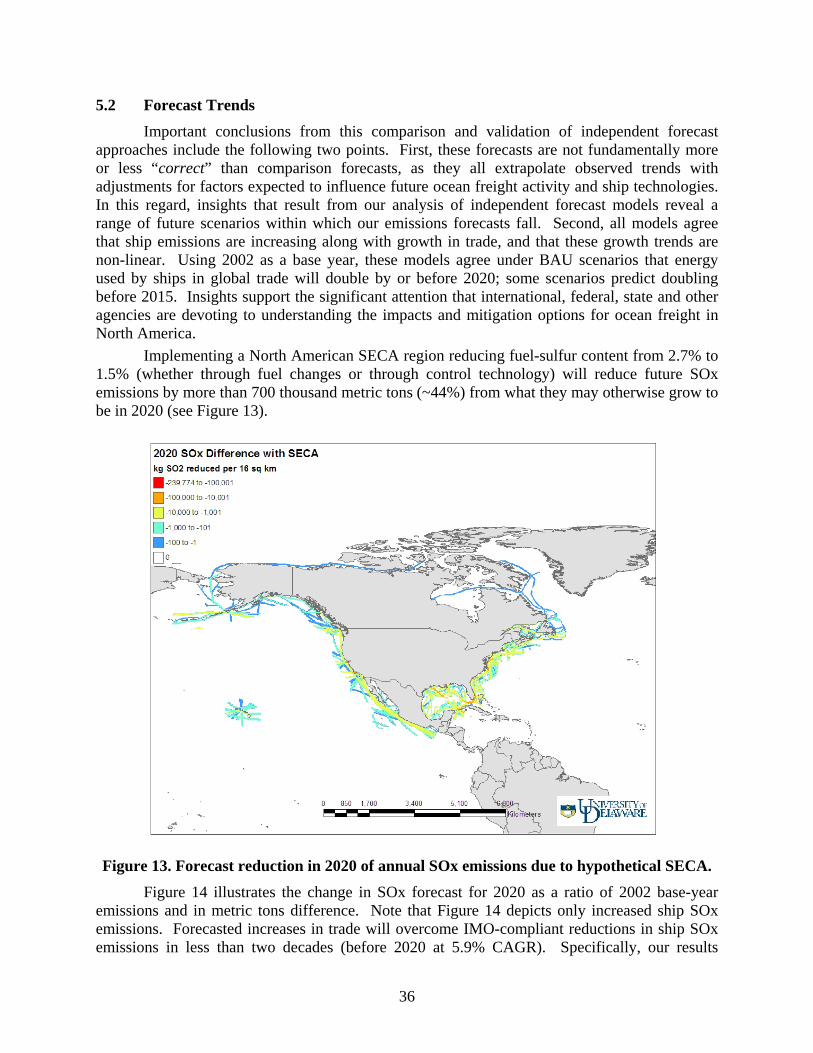
36

5.2 Forecast Trends Important conclusions from this comparison and validation of independent forecast

approaches include the following two points. First, these forecasts are not fundamentally more or less “correct” than comparison forecasts, as they all extrapolate observed trends with adjustments for factors expected to influence future ocean freight activity and ship technologies. In this regard, insights that result from our analysis of independent forecast models reveal a range of future scenarios within which our emissions forecasts fall. Second, all models agree that ship emissions are increasing along with growth in trade, and that these growth trends are non-linear. Using 2002 as a base year, these models agree under BAU scenarios that energy used by ships in global trade will double by or before 2020; some scenarios predict doubling before 2015. Insights support the significant attention that international, federal, state and other agencies are devoting to understanding the impacts and mitigation options for ocean freight in North America.

Implementing a North American SECA region reducing fuel-sulfur content from 2.7% to 1.5% (whether through fuel changes or through control technology) will reduce future SOx emissions by more than 700 thousand metric tons (~44%) from what they may otherwise grow to be in 2020 (see Figure 13).

Figure 13. Forecast reduction in 2020 of annual SOx emissions due to hypothetical SECA. Figure 14 illustrates the change in SOx forecast for 2020 as a ratio of 2002 base-year

emissions and in metric tons difference. Note that Figure 14 depicts only increased ship SOx emissions. Forecasted increases in trade will overcome IMO-compliant reductions in ship SOx emissions in less than two decades (before 2020 at 5.9% CAGR). Specifically, our results

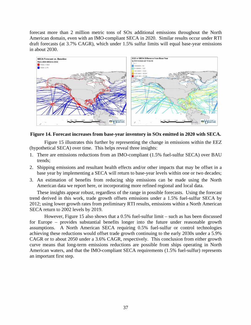
37

forecast more than 2 million metric tons of SOx additional emissions throughout the North American domain, even with an IMO-compliant SECA in 2020. Similar results occur under RTI draft forecasts (at 3.7% CAGR), which under 1.5% sulfur limits will equal base-year emissions in about 2030.

Figure 14. Forecast increases from base-year inventory in SOx emitted in 2020 with SECA. Figure 15 illustrates this further by representing the change in emissions within the EEZ

(hypothetical SECA) over time. This helps reveal three insights: 1. There are emissions reductions from an IMO-compliant (1.5% fuel-sulfur SECA) over BAU

trends; 2. Shipping emissions and resultant health effects and/or other impacts that may be offset in a

base year by implementing a SECA will return to base-year levels within one or two decades; 3. An estimation of benefits from reducing ship emissions can be made using the North

American data we report here, or incorporating more refined regional and local data. These insights appear robust, regardless of the range in possible forecasts. Using the forecast

trend derived in this work, trade growth offsets emissions under a 1.5% fuel-sulfur SECA by 2012; using lower growth rates from preliminary RTI results, emissions within a North American SECA return to 2002 levels by 2019.

However, Figure 15 also shows that a 0.5% fuel-sulfur limit – such as has been discussed for Europe – provides substantial benefits longer into the future under reasonable growth assumptions. A North American SECA requiring 0.5% fuel-sulfur or control technologies achieving these reductions would offset trade growth continuing to the early 2030s under a 5.9% CAGR or to about 2050 under a 3.6% CAGR, respectively. This conclusion from either growth curve means that long-term emissions reductions are possible from ships operating in North American waters, and that the IMO-compliant SECA requirements (1.5% fuel-sulfur) represents an important first step.

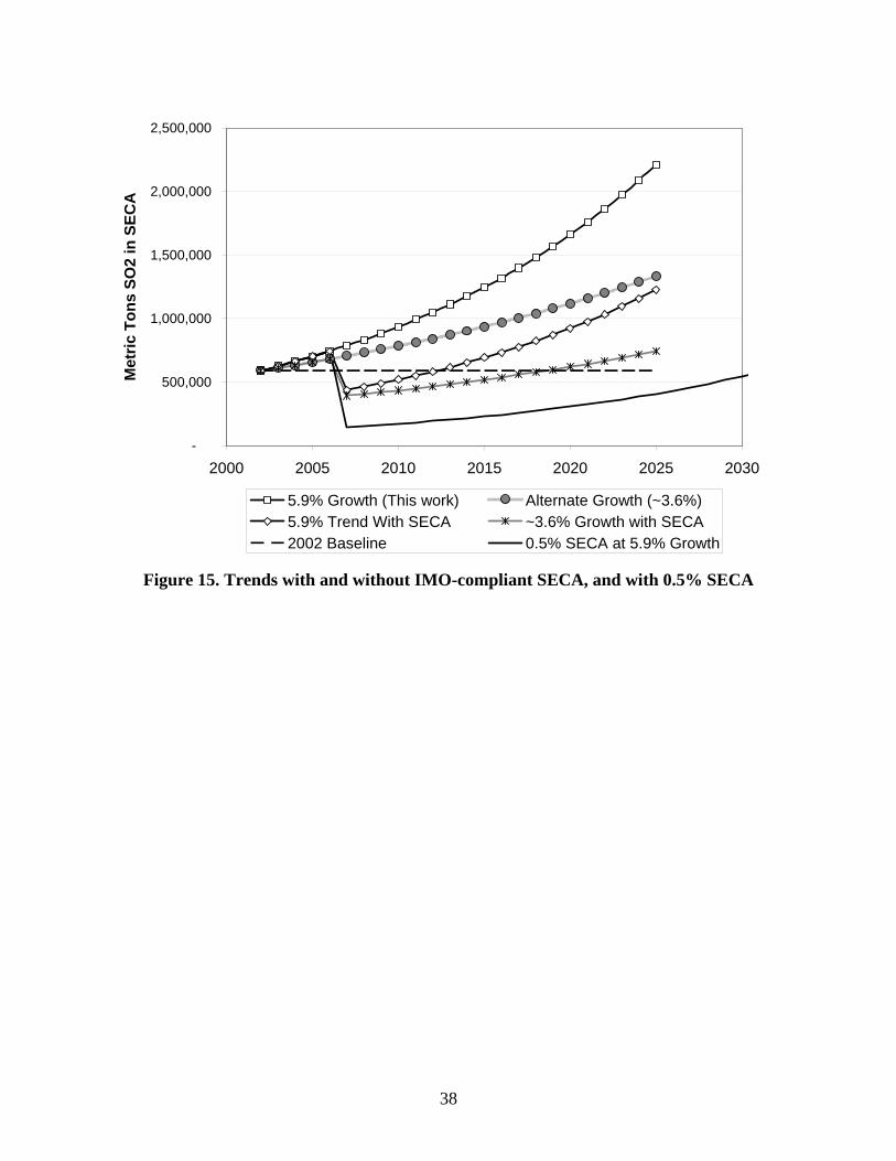
38

-

500,000

1,000,000

1,500,000

2,000,000

2,500,000

2000 2005 2010 2015 2020 2025 2030

Met

ric T

ons

SO2

in S

ECA

5.9% Growth (This work) Alternate Growth (~3.6%)5.9% Trend With SECA ~3.6% Growth with SECA2002 Baseline 0.5% SECA at 5.9% Growth

Figure 15. Trends with and without IMO-compliant SECA, and with 0.5% SECA

39

6.0 RECOMMENDATIONS

6.1 Improve precision The ability of this work to assign interport ship traffic to empirically derived shipping

patterns is an inherent strength of STEEM. However, the precision of this waterway network can be improved – particularly for regions near port. Some of this work is being attempted by U.S. EPA contractors to insert adjustments to the location and intensity of near-port traffic. This limitation is a function of the global context in which the STEEM network was developed, rather than a limitation in model capability. Using global ship location data (ICOADS), a network of shipping lanes was developed; this network could benefit from near-shore comparisons with Automatic Identification System (AIS) data, Vessel Traffic Management Systems (VTMS), or other local information describing near-port routing.

6.2 Reduce Base-Year Uncertainty The baseline inventory effort followed general best practices for calculating emissions

inventories, which enables general analysis of uncertainty due to estimating input parameters, as discussed in the report for Tasks 1 and 2, and elsewhere (100, 101). Results show good agreement with other inventories, including the draft trade-energy model estimate for 2001 by RTI (93). National level uncertainty includes four major elements: A) uncertainty in input parameter assumptions (e.g., emissions factors, engine activity profile, etc.); B) uncertainty in U.S. domestic shipping not included in foreign commerce vessel movement data; C) uncertainty in U.S. Army Corp of Engineers data, and in Canadian and Mexican LMIU data; and D) spatial uncertainty in routing choices, particularly within confined bay and port regions and seasonally for open ocean routes where weather routing may occur. An uncertainty analysis was performed on fundamental input parameters in the model, and potential undercounting of voyages or their misassignment in the routing model was discussed, including opportunities to improve the baseline inventory produced by STEEM for this work.

Figure 16 illustrates the influence of primary inputs on uncertainty for different pollutant estimates. This shows that the uncertainty of output is nearly symmetric, but that the emission factor (i.e., fuel-sulfur content for SO2 and possibly for PM) is the most uncertain input for SO2, PM, HC and CO. For NOx and CO2, similar internal engine combustion conditions (e.g., similar cylinder peak temperatures, pressures, etc.) result in similar emissions factors; this results in greater certainty for emissions factors and relatively greater contribution to variance from uncertainties in engine load, power, and hours of operation. Localized and in-port inventory uncertainties are expected to be larger than national-level bounds estimated here.

6.3 Improve Trend Extrapolation

These forecasts must be considered to represent what other forecast scenarios often refer to as “business as usual” (BAU). The primary uncertainty in the forecast trend applied to the 2002 baseline inventory can be best understood in terms of backcast validation efforts described above. Improving confidence in extrapolated trends for North American ship activity requires longer historic trends, regionally resolved. Improving the nature of extrapolations would require better articulated relationships among drivers and industry trends. However, as shown above, the extrapolated trends developed in this work are within bounded agreement with other forecasts more dependent on trade economics.

40

0% 5% 10% 15% 20% 25% 30% 35% 40%

Engine Load

EmissionsFactor

Power Rating

Operating Hours

Oxides of NitrogenCarbon Dioxide

0% 20% 40% 60% 80% 100%

Engine Load

Fuel Sulfur/Emissions

Factor

Power Rating

OperatingHours

Particulate Matter PM10Sulfur Dioxide

0% 10% 20% 30% 40% 50% 60% 70%

Engine Load

EmissionsFactor

Power Rating

Operating Hours

Carbon MonoxideHydrocarbons

Figure 16. Uncertainty in model output from input parameters scaled by contribution to

output variance. A secondary element in trend uncertainty could reside in missing data fields associating

installed power with ships calling on North America. For this work, we used linear regressions within each vessel type associating gross registered tonnage (GRT) and installed power to fill data gaps. During later review, we compared overall power-based growth trends using net registered tonnage (NRT) regressions. There was less than 0.6% difference between the regressed power and reported power in registry data for 2002, indicating that both GRT and NRT regressions yield similar results. However, as we move back in time, we note empty fields in the GRT data increase faster than empty fields in the NRT data; this could result in different trend estimates for the same historic ship calls. Upon review, we confirmed that using NRT correlations with installed power could increase the 1997 estimates by less than 9%; none of the other years’ installed power totals changed much. This could decrease the overall growth trends used in this work by less than 1%.

We think this uncertainty in trend extrapolation could be worth further research, but acknowledge that revised trends would still compare well in our validation analysis. No major insights or conclusions would change. Ship emissions activity would still be on track to double before 2020 in North America, and an IMO-compliant SECA would still return to 2002 levels within two decades. A lower growth rate in installed power could indicate slightly greater reductions in energy intensity (e.g., faster decoupling of trade and emissions) over time, but this would still be within the 1% to 2% range reported in this work.

41

6.4 Incorporate additional detail among drivers affecting change Underlying drivers of freight activity and the energy systems that produce emissions will

continue to merit analysis. For example, growing GDP may remain highly correlated with growth in imports as it has over past decades. This correlation could become stronger in the future, or one might consider how and whether change in population age and demographics could reduce the rate of consumption and trade in North America without a downturn in GDP. These sorts of effects on global and regional shipping are not considered in this work, either directly or through any of the BAU forecast trends considered; a potential exception could be include work by Eyring et al., which modifies growth on major trade routes greater than recent trends and North American analyses would suggest (39). Better consideration of drivers for change in freight transportation represents a rich area for future research, particularly in terms of goods movement.

6.5 Incorporate planned or proposed signals to modify technological change trends This work explicitly accounts for the expected impacts of NOx emissions limits imposed

by MARPOL Annex VI – already in force, as discussed above. In addition to the Annex VI NOx limits, one could consider including fuel switching measures proposed by the State of California for auxiliary engines and/or in a recent proposal by INTERTANKO (102). We forecast emissions without considering such interventions, to compare BAU results with a SECA regime. This enables atmospheric modeling analyses by members of the North American SECA team to consider what reductions may achieve air quality goals in North America. Future work could consider actions (e.g., emissions trading regimes) that could accelerate or out-perform a SECA for North America; recent work has begun to consider these issues (103).

6.6 Model fleet behavior in response to potential action Few assumptions about influences of EU regulatory activity, IMO decisions, or changes

in marine fuel supply and demand are imposed in forecasts presented here. Moreover, this work assumes full compliance with SECA requirements and no change in fleet logistics associated with these scenarios. Additional modeling of fleet responses to policy or economic signals may reveal motivations for unintended behavior and assess their likelihood. This could help clarify whether increased regulation could deter trade, or whether observations confirming such behavior are mostly anecdotal.

6.7 Extend voyage data or analytical detail Overall the inventories produced for this project using STEEM are shown to be valid

geospatial depictions of emissions from commercial ship activity in North America. Some limitations reveal potential for future analyses to become more accurate and descriptive. Consideration of heterogeneous forecast trends separately for different vessel types and trade routes would produce spatial results revealing asymmetry among future trends for liner trades and bulk trades.

STEEM is a global model that can provide significant insights beyond the North American domain defined for this project. Additionally, STEEM can be run with updated information at multiple scales to produce time series, vessel-type comparisons, or to reveal other characteristics important to understand industry-level effects of alternative mitigation strategies.

42

7.0 REFERENCES 1. Johnson, L.S., Coastal State Regulation of International Shipping. 2004, Dobbs Ferry,

NY: Oceans Publications, Inc. 2. World Shipping Council, Liner Shipping: Facts and Figures. 2006, World Shipping

Council. 3. Corbett, J.J. and P.S. Fischbeck, Emissions from Ships. Science, 1997. 278(5339): p. 823-

824. 4. Corbett, J.J. and H.W. Koehler, Updated Emissions from Ocean Shipping. Journal of

Geophysical Research, 2003. 108(D20): p. 4650. 5. Endresen, Ø., et al., Emission from International Sea Transportation and Environmental

Impact. Journal of Geophysical Research, 2003. 108(D17): p. 4560. 6. Endresen, O., et al., Improved modelling of ship SO2 emissions--a fuel-based approach.

Atmospheric Environment, 2005. 39(20): p. 3621-3628. 7. Streets, D.G., G.R. Carmichael, and R.L. Arndt, Sulfur Dioxide Emissions and Sulfur

Deposition from International Shipping in Asian Waters. Atmospheric Environment, 1997. 31(10): p. 1573-1582.

8. Streets, D.G., S.K. Guttikunda, and G.R. Carmichael, The Growing Contribution of Sulfur Emissions from Ships in Asian Waters 1988-1995. Atmospheric Environment, 2000. 24(26): p. 4425-4439.

9. Corbett, J.J., Emissions from Ships in the Northwestern United States. Environmental Science & Technology, 2002. 36(6): p. 1299-1306.

10. Corbett, J.J. and P.S. Fischbeck, Emissions from Waterborne Commerce Vessels in United States Continental and Inland Waterways. Environmental Science and Technology, 2000. 34(15): p. 3254-3260.

11. Corbett, J.J., P.S. Fischbeck, and S.N. Pandis, Global Nitrogen and Sulfur Emissions Inventories for Oceangoing Ships. Journal of Geophysical Research, 1999. 104(D3): p. 3457-3470.

12. Capaldo, K.P., et al., Effects of Ship Emissions on Sulphur Cycling and Radiative Climate Forcing Over the Ocean. Nature, 1999. 400: p. 743-746.

13. Lawrence, M. and P. Crutzen, Influence of NOx Emissions from Ships on Tropospheric Photochemistry and Climate. Nature, 1999. 402(6758): p. 167-170.

14. International Maritime Organization, Report on the outcome of the IMO Study on Greenhouse Gas Emissions from Ships. MEPC 45/8, 2000.

15. International Maritime Organization. Designation of the North Sea area as a SOx Emission Control Area. in MEPC 44/11/4. 1999.

16. Jonson, J.E., L. Tarrason, and J. Bartnicki, Effects of international shipping on European pollution levels. 2000, The Norwegian Metrorological Institute.

17. Commission of the European Communities and Entec UK Limited, Quantification of Emissions from Ships Associated with Ship Movements between Ports in the European Community. 2002, European Commission.

18. Isakson, J., T.A. Persson, and E. Selin Lindgren, Identification and assessment of ship emissions and their effects in the harbour of Goteborg, Sweden. Atmospheric Environment, 2001. 35(21): p. 3659-3666.

19. Kesgin, U. and N. Vardar, A study on exhaust gas emissions from ships in Turkish Straits. Atmospheric Environment, 2001. 35(10): p. 1863-1870.

43

20. Bailey, D. and G. Solomon, Pollution prevention at ports: clearing the air. Environmental Impact Assessment Review, 2004. 24(7-8): p. 749-774.

21. Murphy, T.M., et al. The Need to Reduce Marine Shipping Emissions: A Santa Barbara County Case Study. in Air & Waste Management Association Conference. 2003.

22. CONCAWE, The contribution of sulphur dioxide emissions from ships to coastal deposition and air quality in the channel and the southern north sea area. 1994: Brussels.

23. U.S. Environmental Protection Agency, Final Regulatory Support Document: Control of Emissions from New Marine Compression-Ignition Engines at or Above 30 Liters per Cylinder. 2003.

24. Lloyd's Register, Marine Exhaust Emissions Quantification Study - Mediterranean Sea. 1999.

25. Lloyd's Register and International Maritime Organization, Marine Exhaust Emission Quantification Study - Baltic Sea, in MEPC 45/INF.7. 1998.

26. Environmental Protection Agency, Inventory of U.S. Greenhouse Gas Emissions and Sinks: 1990-2003. 2005, U.S. Environmental Protection Agency: Washington, DC. p. 432.

27. Environmental Protection Agency, National Air Pollutant Emission Trends, 1970-2002. 2005, U.S. Environmental Protection Agency: Washington, DC.

28. Bates, J., et al., Economic Evaluation of Emissions Reductions in the Transport Sector of the EU: Bottom-up Analysis, UPDATED, Final Report. 2001, AEA Technology Environment: Abingdon, UK.

29. California Air Resources Board, Proposed 2003 State and Federal Strategy for California SIP. 2003, California Environmental Protection Agency: Sacramento, CA. p. 157.

30. Corbett, J.J. and H.W. Koehler, Considering alternative input parameters in an activity-based ship fuel consumption and emissions model: Reply to comment by Øyvind Endresen et al. on ‘‘Updated emissions from ocean shipping’’. Journal of Geophysical Research, 2004. 109(D23303).

31. Endresen, Ø., et al., Substantiation of a lower estimate for the bunker inventory: Comment on ‘‘Updated emissions from ocean shipping’’ by James J. Corbett and Horst W. Koehler. Journal of Geophysical Research, 2004. 109(D23302).

32. Wang, C. and J.J. Corbett, Geographical Characterization of Ship Traffic and Emissions. Transportation Research Record: Journal of the Transportation Research Board, 2005. 1909.

33. Olivier, J.G.J. and J.A.H.W. Peters, International Marine and Aviation Bunker Fuel: Trends, Ranking of Countries and Comparison with National CO2 Emissions. 1999, RIVM.

34. ICF Consulting, Best Practices in Preparing Port Emission Inventories: Draft for Review. 2005, Prepared for Office of Policy, Economics and Innovation, United States Environmental Protection Agency: Fairfax, Virginia. p. 39.

35. Wang, C., J.J. Corbett, and J. Firestone. Adapting Bottom-up Methods to Top-down Spatially Resolved Ship Emissions Inventories. in Transportation Research Board of the National Academies 85th Annual Meeting. 2006. Washington D.C.

36. International Maritime Organization, Annex VI of MARPOL 73/78 and NOx Technical Code. IMO-664E ed. 1998, London, UK: International Maritime Organization. 150.

44

37. Skjølsvik, K.O., et al., Study of Greenhouse Gas Emissions from Ships (MEPC 45/8 Report to International Maritime Organization on the outcome of the IMO Study on Greenhouse Gas Emissions from Ships). 2000, MARINTEK Sintef Group, Carnegie Mellon University, Center for Economic Analysis, and Det Norske Veritas: Trondheim, Norway.

38. European Commission and ENTEC UK Limited, Quantification of emissions from ships associated with ship movements between ports in the European Community. 2002, European Commission, DG ENV.C1, Rue de la Loi, 200, B-1049: Brussels, Belgium.

39. Eyring, V., et al., Emissions from international shipping: 2. Impact of future technologies on scenarios until 2050. Journal of Geophysical Research - Atmospheres, 2005. 110(D17): p. D17306.

40. Ceuster, G.D., B.v. Herbruggen, and S. Logghe, TREMOVE: Description of model and baseline version 2.41, Draft Report, TRANSPORT & MOBILITY LEUVEN, Editor. 2006, European Commission: Brussels, Belgium.

41. Zeebroeck, B.V., G.D. Ceuster, and B.V. Herbruggen, TREMOVE 2: Maritime model and runs, TRANSPORT & MOBILITY LEUVEN, Editor. 2006, European Commission: Brussels, Belgium.

42. Environmental Protection Agency, 40 CFR Parts 9 and 94: Control of Emissions From New Marine Compression-Ignition Engines at or Above 30 Liters per Cylinder: Final Rule. 2003, Federal Register: Washington, DC. p. 96.

43. Environmental Protection Agency, Final Regulatory Impact Analysis: Control of Emissions From Compression-Ignition Marine Engines. 1999, U.S. EPA Office of Air and Radiation; Office of Mobile Sources; Engine Programs and Compliance Division: Ann Arbor, MI. p. 132.

44. Environmental Protection Agency, 40 CFR Parts 89, 92, and 94: Control of Emissions of Air Pollution from New CI Marine Engines at or above 37 kW: Final Rule. 1999, Federal Register: Washington, DC.

45. U.S. Department of Transportation, Research and Innovative Technology Administration, and Bureau of Transportation Statistics, North American Freight Transportation. 2006, Bureau of Transportation Statistics: Washington, DC: 2006.

46. Bureau of Economic Analysis, Table 1.1.6. Real Gross Domestic Product, Chained Dollars, in National Income and Product Accounts Tables. 2006, U.S. Department of Commerce: Washington, DC. p. Today is: 11/3/2006 Last Revised on October 27, 2006 Next Release Date November 29, 2006.

47. TRB Executive Committee, G. Giuliano, and S. Godwin, Critical Issues in Transportation. 2006, Transportation Research Board: Washington, DC. p. 12.

48. Vickerman, J., North American Marine Trade and Transportation Trends, in Transystems Industry Presentations. 2006: Kansas City, MO.

49. Port of Los Angeles (POLA) and Port of Long Beach (POLB), San Pedro Bay Ports Clean Air Action Plan Technical Report: Final. 2006, Port of Los Angeles (POLA) and Port of Long Beach (POLB): Los Angeles and Long Beach, CA. p. 262.

50. NNI Task Force, Report to Mayor Hahn and Councilwoman Hahn by the No Net Increase Task Force. 2005, Port of Los Angeles: Los Angeles, CA. p. 603.

51. Mercator Transport Group, Herbert Engineering Corporation, and MDS Transmodal Ltd, Forecast of Container Vessel Specifications and Port Calls Within San Pedro Bay: Final Report. 2005, Cunningham Report: Bellevue, WA. p. 139.

45

52. Meyer Mohaddes Associates Inc., Port of Los Angeles Baseline Transport Study. 2004, Port of Los Angeles: Los Angeles. p. 70.

53. Parsons Transportation Group, San Pedro Bay Ports Rail Market Study, TM-1b, Draft Report. 2004, Port of Los Angeles: Los Angeles. p. 30.

54. Port of Los Angeles, et al., Control of Ship Emission in the South Coast Air Basin: Assessment of the Proposed Federal Implementation Plan Ship Fee Emission Fee Program. 1994, Port of Los Angeles: Los Angeles, CA.

55. California Air Resources Board, Goods Movement and Ports. 2006, California Air Resources Board: Sacramento, CA.

56. Southern California Association of Governments, Goods Movement. 2006, Southern California Association of Governments: Los Angeles, CA.

57. Port of Los Angeles, Goods Movement Projects. 2006. 58. U.S. Environmental Protection Agency and ARCADIS Geraghty & Miller Inc.,

Commercial Marine Activity for Deep Sea Ports in the United States. 1999, Assessment and Modeling Division, Office of Mobile Sources, Environmental Protection Agency: Ann Arbor, Michigan.

59. U.S. Environmental Protection Agency and ARCADIS Geraghty & Miller Inc., Commercial Marine Activity for Great Lake and Inland River Ports in the United States. 1999, Assessment and Modeling Division, Office of Mobile Sources, Environmental Protection Agency: Ann Arbor, Michigan.

60. Wang, C., A Study of Geographical Characterization of Ship Traffic and Emissions and Cost-effectiveness of Reducing Sulfur Emissions from Foreign Waterborne Commerce for the U.S. West Coast, in College of Marine Studies. 2006, University of Delaware: Newark.

61. U.S. Army Corps of Engineers, Vessel Entrances and Clearances. 2004, Waterborne Commerce Statistics Center, U.S. Army Corps of Engineers.

62. Lloyds Maritime Intelligence Unit, Commercial marine vessel activity data in Canada for the years 1995 through 2005. Various 1996-2004: London, United Kingdom.

63. Lloyds Maritime Intelligence Unit, Commercial marine vessel activity data in Mexico for the years 1996, 1998, 2000, 2002, and 2004. Various 1996-2004: London, United Kingdom.

64. Lloyds Maritime Information System (LMIS), The Lloyds Maritime Database. 2002, Lloyd's Register - Fairplay Ltd.

65. Corbett, J.J., Verification of Ship Emission Estimates with Monitoring Measurements to Improve Inventory and Modeling. 2004, University of Delaware: Newark, DE. p. 47.

66. UNCTAD, Review of Maritime Transport 2003. 2003, United Nations: Geneva. p. 158. 67. UNCTAD, Review of Maritime Transport 2002. 2002, United Nations: Geneva. p. 145. 68. UNCTAD, Review of Maritime Transport 1994. 1995, United Nations: New York and

Geneva. 69. UNCTAD, Review of Maritime Transport 2006. 2006, United Nations: Geneva. p. 160. 70. MARAD, Website pages. 2006, U.S. Maritime Administration, Department of

Transportation: Washington, DC. 71. American Association of Port Authorities (AAPA), U.S./Canada Container Traffic in

TEUs 1980-2005. 2006, AAPA: Alexandria, VA. p. spreadsheet sent from MARAD and similar found on website.

46

72. Corbett, J.J. and H.W. Koehler, Updated Emissions from Ocean Shipping. Journal of Geophysical Research - Atmospheres, 2003. 108(D20): p. 4650-4666.

73. UNFCCC and Subsidiary Body for Scientific and Technological Advice, Methodological issues relating to emissions from international aviation and maritime transport; Note by the secretariat. 2004, United Nations Framework Convention on Climate Change, Subsidiary Body for Scientific and Technological Advice: Bonn, Germany. p. 11.

74. Corbett, J.J., Marine Transportation and Energy Use, in Encyclopedia of Energy, C.J. Cleveland, Editor. 2004, Elesvier Science: San Diego, CA. p. 745-748.

75. California Air Resources Board, Emissions Estimation Methodology for Ocean-Going Vessels. 2005.

76. Levelton Consultants Ltd., Marine Emission Inventory Study Eastern Canada and Great Lakes - Interim Report 4: Gridding Results. 2006, Prepared for: Transportation Development Centre Transport Canada.

77. U.S. Environmental Protection Agency, Latest Findings on National Air Quality: 2002 Status and Trends. 2003.

78. NOAA Office of Coast Survey, Exclusive Economic Zone. 2004. 79. Aldrete, G., et al., Port-wide Baseline Air Emissions Inventory Prepared for Port of Los

Angeles. 2004, Starcrest Consulting Group, LLC. 80. Anderson, B.E. and J.L. Ray, Houston-Galveston Area Vessel Emissions Inventory. 2002,

Starcrest Consulting Group, LLC. 81. Anderson, B. and S. Wells, The New York, Northern New Jersey, Long Island

Nonattainment Area Commercial Marine Vessel Emissions Inventory. 2003, Starcrest Consulting Group, LLC.

82. Levelton Engineering Ltd., Marine Vessel Air Emissions in B.C. and Washington State outside the GVRD and FVRD for the Year 2000. 2002.

83. Stopford, M., Maritime Economics. Second ed. 1997, London, UK: Routledge, Taylor and Francis Group. 562.

84. US Army Corps of Engineers, Waterborne Commerce of the United States: Part 5 – National Summaries. 2005, U.S. Army Corps of Engineers: Alexandria, Virginia. p. 100.

85. Le Dam Hanh, P.I., The Logistics of Empty Cargo Containers in the Southern California Region: Are Current International Logistics Practices a Barrier to Rationalizing the Regional Movement of Empty Containers? 2003, METRANS Transportation Center, University of Southern California, and California State University, Long Beach: Long Beach, CA. p. 40.

86. Slater, R. and MTS Task Force, An Assessment of the U.S. Marine Transportation System: A Report to Congress. 1999, Washington, DC: U.S. Department of Transportation. 104.

87. Federal Highway Administration and B. Lambert, Freight Analysis Framework Overview. 2002, Federal Highway Administration: Washington, DC. p. 2.

88. U.S. Environmental Protection Agency, et al., MOVES2004 Highway Vehicle Population and Activity Data, Draft. 2004, U.S. Environmental Protection Agency: Washington, DC. p. 99.

89. Bureau of Transportation Statistics, Pocket Guide to Transportation. 2004, Bureau of Transportation Statistics: Washington, DC. p. 52.

47

90. U.S. Environmental Protection Agency, Locomotive Emissions Standards Regulatory Support Document. 1998, U.S. Environmental Protection Agency: Washington, DC. p. 127.

91. Dennis, S.M., Improved Estimates of Ton-Miles. Journal of Transportation and Statistics, 2005. 8(1).

92. Davis, S., Transportation Energy Data Book: Edition 23. 2003, Oak Ridge National Laboratory: Oak Ridge, TN.

93. RTI International, et al., Meeting discussions of preliminary model design and results for trade energy model, related to RTI Project Number 0209701.001, Upublished Results, J.J. Corbett and California Air Resources Board, Editors. 2006: Washington, DC.

94. Corbett, J.J., Environmental Impacts of Ocean Shipping in a Freight Context: A Summary of Current Assessments, Future Trends, and Approaches to Mitigation, Draft, Working Group on Transport, Editor. 2006, Organisation for Economic Cooperation and Development (OECD): Paris, France.

95. Wartsila NSD and K. Heim, Forward look at future emissions control measures for Sulzer RTA engines, in Marine News. 2001, Wartsila NSD: Helsinki, Finland. p. 4.

96. Levelton Engineering Ltd, et al., Marine Emission Inventory Study, Eastern Canada And Great Lakes, Final Report, Levelton Engineering Ltd and Maritime Innovation, Editor. 2006, Transport Canada: Montreal, Quebec. p. 74.

97. Corbett, J.J. and H.W. Koehler, Considering Alternative Input Parameters In An Activity-Based Ship Fuel Consumption And Emissions Model. Journal of Geophysical Research - Atmospheres, 2004. 109(D23303): p. 8.

98. Eyring, V., et al., Emissions from international shipping: 1. The last 50 years. Journal of Geophysical Research - Atmospheres, 2005. 110(D17): p. D17305.

99. Endresen, Ø., et al., Substantiation of a Lower Estimate for the Bunker Inventory: Comment on ‘‘Updated emissions from ocean shipping’’ by James J. Corbett and Horst W. Koehler. Journal of Geophysical Research - Atmospheres, 2004. 109(D23302).

100. Corbett, J.J., C. Wang, and J. Firestone, Estimation, Validation, And Forecasts Of Regional Commercial Marine Vessel Inventories, Tasks 1 And 2: Baseline Inventory And Ports Comparison, Final Report. 2006, State of California Air Resources Board and Commission for Environmental Cooperation of North America: Sacramento, CA, and Montreal, Quebec. p. 42.

101. Wang, C., J.J. Corbett, and J. Firestone, Modeling Energy Use and Emissions from North American Shipping: an Application of Ship Traffic, Energy and Environment Model. Environmental Science & Technology, 2006. under review.

102. Intertanko, Revisions of MARPOL Annex VI, the NOx Technical Code and Relevant Guidelines, in Intersessional Meeting of the BLG-WGAP, BLG Working Group on Air Pollution, IMO submittal, Editor. 2006, INTERSESSIONAL MEETING OF THE BLG WORKING GROUP ON AIR POLLUTION, 1st session, Agenda item 2: London, UK.

103. Wang, C., J.J. Corbett, and J.J. Winebrake, Reducing Sulfur Emissions from Ships. 2006. in preparation.

48

LIST OF ACRONYMS

AAPA American Association of Port Authorities AE Auxiliary Engine AIS Automatic Identification System AMVER Automated Mutual Vessel Emergency Response ARB California Air Resources Board BAU Business as usual BTS U.S. Bureau of Transportation Statistics CAGR Compound annual growth rate CEC Commission for Environmental Cooperation of North America CMV Commercial Marine Vessel CO Carbon monoxide CO2 Carbon dioxide COADS Comprehensive Ocean-Atmosphere Data Set (now ICOADS) EEZ Exclusive Economic Zones EF Emissions factor GDP Gross Domestic Product GIS Geographic Information System GRT Gross Registered Tonnage HC Hydrocarbon HFO Heavy fuel oil IMO International Maritime Organization ICOADS International Comprehensive Ocean-Atmosphere Data Set INTERTANKO Independent Tanker Owners And Operators kW Kilowatts LMIU Lloyds Maritime Intelligence Unit MARAD U.S. Maritime Administration MARPOL Maritime Pollution Convention MDO Marine distillate oil MOVES U.S. EPA Mobile Vehicle Emissions Simulator NESCAUM Northeast States for Coordinated Air Use Management NNI No net increase NRT Net Register Tonnage NOx Oxides of nitrogen PM Particulate matter RTI Research Triangle Institute, Inc. SECA SOx Emission Control Area SFOC Specific fuel oil consumption SOx Oxides of sulfur STEEM Waterway Network Ship Traffic, Energy and Environment Model TREMOVE Transportation and environment policy assessment model (European Commission) USACE U.S. Army Corps Engineers U.S. EPA United States Environmental Protection Agency

49

Appendix: Summary of North American Ports and Waterways There are over 400 North American ports and waterways; these ports connect about with

~1,300 foreign ports in the 2002 U.S. Entrances and Clearances data set; about 950 ports are in the 2002 Lloyd’s movement data set, with some overlapping ports among Canada, Mexico, and the United States. These ports are located based on longitude and latitude and connected to the STEEM network in ArcMap. The following tables summarize ports and waterways from input data for the United States, Canada, and Mexico, respectively. These are listed according to descending order of port calls, by percentage. Because of some duplicate voyages where arrivals in some ports represent departures in other ports, we do not report absolute counts of port calls from these input data (estimated from STEEM to be ~172,000 for North America in 2002) and we do not merge these into one North American ranking.

Table A1 and Table A2 represent U.S. ports and waterways as reported in USACE foreign commerce data. Thirty-seven states and some 250 ports and waterways are represented in U.S. Foreign Commerce data. The top 12 states and the top 50 ports and waterway locations account for more than 80% of U.S. foreign commerce ship calls, respectively.

Table A3 represents Canadian ports as provided in LMIU data. The top 21 of 150 ports represent more than 80% of Canadian ship calls.

Table A4 represents Mexican ports as provided in LMIU data. The top 7 of 42 ports represent more than 80% of Mexican ship calls.

50

Table A-1. State-by-state Summary of Ports and Port Calls

Rank by Foreign Commerce Port Calls US State or Region

Ports and Waterways in

Input Data Percent of U.S. Calls Cumulative Percent 1 Florida 14 16.18% 16.18% 2 Texas 12 12.90% 29.08% 3 Louisiana 9 9.94% 39.02% 4 California 17 9.59% 48.60% 5 Washington 13 6.62% 55.22% 6 New York/New Jersey 1 5.20% 60.43% 7 Virgin Islands 6 4.94% 65.37% 8 Puerto Rico 9 3.92% 69.29% 9 Alaska 35 3.41% 72.69%

10 Georgia 2 2.99% 75.68% 11 Virginia 9 2.77% 78.45% 12 South Carolina 3 2.64% 81.09% 13 Maryland 2 2.08% 83.17% 14 Michigan 29 1.54% 84.71% 15 Ohio 10 1.37% 86.08% 16 Alabama 3 1.32% 87.40% 17 Oregon 4 1.29% 88.68% 18 Pennsylvania 5 1.27% 89.95% 19 Mississippi 3 1.20% 91.15% 20 Hawaii 7 1.19% 92.34% 21 Maine 7 1.16% 93.50% 22 Massachusetts 7 1.06% 94.57% 23 New Jersey 5 1.00% 95.57% 24 North Carolina 4 0.73% 96.30% 25 Delaware 3 0.59% 96.89% 26 Minnesota and Wisconsin 1 0.59% 97.48% 27 Connecticut 3 0.42% 97.89% 28 Louisiana and Texas 1 0.27% 98.17% 29 New York 4 0.27% 98.44% 30 Rhode Island 2 0.23% 98.67% 31 Gulf 1 0.21% 98.88% 32 Maine and New Hampshire 1 0.20% 99.08% 33 Great Lakes 2 0.19% 99.27% 34 Indiana 3 0.18% 99.45% 35 Illinois 2 0.17% 99.62% 36 Wisconsin 1 0.13% 99.75% 37 New York 6 0.11% 99.86% 38 Maryland and Virginia 1 0.07% 99.93% 39 Michigan and Wisconsin 1 0.06% 99.99% 40 Minnesota 1 0.01% 100.00% 41 Washington, DC 1 0.00% 100.00% 42 Minnesota 1 0.00% 100.00%

Grand Total 251 100.00%

51

Table A-2. U.S. Port and Waterway Summary from USACE Foreign Commerce Data

Rank by Foreign Commerce Port Calls US Port/Waterway Name Percent of U.S. Calls Cumulative Percent

1 Houston 5.64% 5.64% 2 Port Of New York 5.20% 10.84% 3 Miami Harbor 4.95% 15.79% 4 Port Everglades Harbor 4.16% 19.95% 5 San Juan Harbor 2.99% 22.94% 6 Port Of New Orleans 2.98% 25.91% 7 Los Angeles Harbor 2.74% 28.65% 8 Long Beach Harbor 2.59% 31.24%

9 Charleston Harbor (Including Ashley River, Cooper River, Shem Creek) 2.52% 33.76%

10 St. Thomas Harbor 2.51% 36.27% 11 Savannah Harbor 2.42% 38.70% 12 Seattle Harbor 2.35% 41.04% 13 Port Of South Louisiana 2.16% 43.20% 14 Baltimore Harbor And Channels 2.07% 45.28% 15 Elizabeth River 1.99% 47.27%

16 Bayou Lafourche And Lafourche-Jump Waterway 1.93% 49.20%

17 Tacoma Harbor 1.79% 50.99% 18 Oakland Harbor 1.71% 52.70% 19 Jacksonville Harbor 1.67% 54.36% 20 Galveston Channel 1.59% 55.95% 21 Beaumont 1.40% 57.35% 22 Corpus Christi 1.39% 58.74% 23 Tampa Harbor 1.39% 60.12% 24 Palm Beach Harbor 1.38% 61.50% 25 Mobile Harbor 1.23% 62.73% 26 Port Of Portland 1.12% 63.86% 27 Port Of Boston 0.94% 64.80% 28 San Diego Harbor 0.92% 65.72% 29 Canaveral Harbor 0.92% 66.64% 30 Texas City Channel 0.91% 67.54% 31 Port Hess St. Croix Island 0.90% 68.45% 32 Freeport Harbor 0.88% 69.33% 33 Calcasieu River And Pass (Lake Charles) 0.84% 70.18% 34 Ketchikan Harbor 0.84% 71.02%

35 Atchafalaya River (Morgan City To Gulf Of Mexico) 0.73% 71.75%

36 Port Of Baton Rouge 0.69% 72.43% 37 Philadelphia Harbor 0.68% 73.12% 38 Honolulu Harbor, Oahu 0.62% 73.74% 39 Key West Harbor 0.62% 74.35% 40 Delaware River At Camden 0.59% 74.95% 41 Duluth-Superior Harbor 0.59% 75.54% 42 Port Of Plaquemines 0.59% 76.12% 43 Pascagoula Harbor 0.57% 76.69%

52

Rank by Foreign Commerce Port Calls US Port/Waterway Name Percent of U.S. Calls Cumulative Percent

44 East River And Oglethorpe Bay 0.57% 77.26% 45 Port Of Wilmington 0.52% 77.78% 46 Juneau Harbor 0.52% 78.31% 47 Port Harvey St. Croix Island 0.52% 78.83% 48 Port Arthur 0.51% 79.34% 49 St. John Island 0.48% 79.82% 50 Christiansted Harbor, St. Croix 0.47% 80.30% 51 Anacortes Harbor 0.45% 80.74% 52 Port Of Newport News 0.42% 81.16% 53 Wilmington Harbor 0.42% 81.58% 54 Other Puget Sound Area Ports 0.41% 81.99% 55 Gulfport Harbor 0.40% 82.39% 56 Portland Harbor 0.40% 82.79% 57 Ponce Harbor 0.39% 83.19% 58 Toledo Harbor 0.39% 83.58% 59 Skagway Harbor 0.38% 83.96% 60 Everett Harbor And Snohomish River 0.37% 84.33% 61 Port Manatee 0.37% 84.70% 62 Port Hueneme 0.36% 85.05% 63 Conneaut Harbor 0.35% 85.40% 64 Matagorda Ship Channel 0.34% 85.75% 65 Rouge River 0.34% 86.09% 66 Paulsboro 0.32% 86.42% 67 Port Of Vancouver 0.32% 86.74% 68 Fernandina Harbor 0.31% 87.05% 69 Unalaska Bay And Island 0.31% 87.36% 70 Cleveland Harbor 0.30% 87.66% 71 Richmond Harbor 0.29% 87.95% 72 Kivilina 0.29% 88.24% 73 Eastport Harbor 0.28% 88.52%

74 Gulf Intracoastal Waterway, Mississippi River, LA, To Sabine River, TX 0.27% 88.79%

75 Port Of Longview 0.27% 89.06% 76 New Haven Harbor 0.27% 89.33% 77 Fore River 0.27% 89.59% 78 Marcus Hook 0.26% 89.85% 79 Mayaguez Harbor 0.25% 90.10% 80 Carquinez Strait 0.24% 90.34% 81 East Pearl River 0.23% 90.57% 82 Sitka Harbor 0.23% 90.80% 83 Port Angeles Harbor 0.22% 91.02% 84 Gulf Via Tiger Pass 0.21% 91.23% 85 Port Huron 0.21% 91.44% 86 Chester Area 0.21% 91.65% 87 Piscataqua River And New Hampshire 0.20% 91.85% 88 Brownsville 0.20% 92.04% 89 San Francisco Harbor 0.18% 92.22%

53

Rank by Foreign Commerce Port Calls US Port/Waterway Name Percent of U.S. Calls Cumulative Percent

90 Sandusky Harbor 0.18% 92.40% 91 Other Hawaiian Islands Area Ports 0.18% 92.58% 92 Grays Harbor And Chehalis River 0.17% 92.75% 93 Elizabeth River (Southern Branch) 0.17% 92.91% 94 Port Of Kalama 0.16% 93.08% 95 Providence River And Harbor 0.16% 93.24% 96 Fort Pierce Harbor 0.15% 93.40% 97 Port Of Chicago 0.15% 93.55% 98 Hilo Harbor, Hawaii Is. 0.14% 93.69% 99 Stockton 0.14% 93.83%

100 Morehead City Harbor 0.14% 93.96% 101 Milwaukee Harbor 0.13% 94.10% 102 Bridgeport Harbor 0.13% 94.23% 103 Ecorse 0.13% 94.36% 104 Burns Waterway Harbor 0.12% 94.48% 105 Detroit Harbor 0.12% 94.60% 106 El Segundo 0.12% 94.73% 107 Lower Delaware Bay 0.12% 94.85% 108 Oswego Harbor 0.12% 94.97% 109 Seward Harbor 0.12% 95.08% 110 Guayanilla Harbor 0.12% 95.20% 111 Nikishka 0.12% 95.31% 112 Searsport Harbor 0.11% 95.43% 113 Panama City Harbor 0.11% 95.54% 114 Georgetown Harbor 0.11% 95.65% 115 Coos Bay 0.11% 95.76% 116 Wrangell Harbor 0.11% 95.86% 117 Nawiliwili Harbor, Kauai 0.10% 95.97% 118 Penn Manor Area 0.10% 96.07% 119 Anchorage 0.10% 96.17% 120 Manistee Harbor 0.10% 96.27% 121 Presque Isle Harbor 0.10% 96.36% 122 Bar Harbor 0.10% 96.46% 123 Lake Huron 0.09% 96.55% 124 Lake Michigan 0.09% 96.65% 125 San Joaquin River 0.08% 96.73% 126 Calcite 0.08% 96.81% 127 Pensacola Harbor 0.08% 96.89% 128 Whittier Harbor 0.08% 96.98% 129 Kahului Harbor, Maui 0.07% 97.05% 130 Dauphin Island Bay 0.07% 97.12% 131 Barbers Point 0.07% 97.19% 132 Port Of Richmond 0.07% 97.26% 133 Fajardo Harbor 0.07% 97.32% 134 Chesapeake Bay 0.07% 97.39% 135 Sacramento 0.07% 97.46% 136 Haines 0.06% 97.52%

54

Rank by Foreign Commerce Port Calls US Port/Waterway Name Percent of U.S. Calls Cumulative Percent

137 Narragansett Bay 0.06% 97.58% 138 Old Tampa Bay 0.06% 97.65% 139 Salem River 0.06% 97.71% 140 Ashtabula Harbor 0.06% 97.77% 141 Homer 0.06% 97.83% 142 Port Of Albany 0.06% 97.89% 143 Humboldt Harbor And Bay 0.06% 97.95% 144 Bellingham Bay And Harbor 0.06% 98.01% 145 Northeast (Cape Fear) River 0.06% 98.06% 146 Menominee Harbor And River 0.06% 98.12% 147 New Castle Area 0.05% 98.17% 148 Port Of Astoria 0.05% 98.23% 149 Port Of Buffalo 0.05% 98.28% 150 Jobos Harbor 0.05% 98.33% 151 Port Of Hopewell 0.05% 98.38% 152 Fall River Harbor 0.05% 98.42% 153 Algonac 0.04% 98.47% 154 Yabucoa Harbor 0.04% 98.51% 155 Frederiksted St. Croix Island 0.04% 98.55% 156 Rochester (Charlotte) Harbor 0.04% 98.60% 157 Sabine Pass Harbor 0.04% 98.64% 158 Sault Ste. Marie 0.04% 98.68% 159 Marysville 0.04% 98.72% 160 Suisun Bay Channel 0.04% 98.76% 161 Little River (Creek) 0.04% 98.79% 162 New Bedford And Fairhaven Harbor 0.04% 98.83% 163 Alexandria Bay 0.03% 98.86% 164 Olympia Harbor 0.03% 98.90% 165 St. Clai 0.03% 98.93% 166 Fairport Harbor 0.03% 98.97% 167 Redwood City Harbor, Ca 0.03% 99.00% 168 Monroe Harbor 0.03% 99.03% 169 Port Dolomite 0.03% 99.06% 170 Port Inland 0.03% 99.09% 171 York River 0.03% 99.12% 172 Adak Island 0.03% 99.15% 173 Indiana Harbor 0.03% 99.18% 174 Akutan Island 0.03% 99.21% 175 Lorain Harbor 0.03% 99.24% 176 Trenton 0.03% 99.27% 177 Alpena Harbor 0.03% 99.29% 178 Charlevoix Harbor 0.03% 99.32% 179 Ogdensburg Harbor 0.03% 99.35% 180 Gary Harbor 0.02% 99.37% 181 Hudson River 0.02% 99.40% 182 New London Harbor 0.02% 99.42% 183 Northville, L.I. 0.02% 99.44%

55

Rank by Foreign Commerce Port Calls US Port/Waterway Name Percent of U.S. Calls Cumulative Percent

184 Marblehead 0.02% 99.46% 185 Michoud Canal 0.02% 99.48% 186 San Pablo Bay And Mare Island Strait 0.02% 99.50% 187 Stoneport 0.02% 99.52% 188 Waukegan Harbor 0.02% 99.54% 189 Detroit District Small Ports - Lake Michigan 0.02% 99.56% 190 Erie Harbor 0.02% 99.58% 191 Hoonah Harbor 0.02% 99.60% 192 Kingston Harbor (North Plymouth) 0.02% 99.61% 193 Muskegon Harbor 0.02% 99.63% 194 Bayou La Batre 0.02% 99.65% 195 Drummond Island 0.02% 99.67% 196 Kodiak Island 0.02% 99.68% 197 Ludington Harbor 0.02% 99.70% 198 Salem Harbor 0.02% 99.72% 199 Escanaba 0.01% 99.73% 200 Port Royal Harbor 0.01% 99.74% 201 Afognak Bay 0.01% 99.76% 202 Burlington-Florence-Roebling 0.01% 99.77% 203 Chignik Bay 0.01% 99.78% 204 Southport 0.01% 99.79% 205 Intracoastal Waterway, Jacksonville To Miami 0.01% 99.80% 206 St. Paul Island, Pribilof Island 0.01% 99.81% 207 Icy Bay 0.01% 99.83%

208 Inland Wtwy From Franklin To The Mermentau River 0.01% 99.84%

209 Togiak Bay 0.01% 99.85% 210 Two Harbors (Agate Bay) 0.01% 99.86% 211 Detour And Vicinity 0.01% 99.86% 212 Penobscot River 0.01% 99.87% 213 Catalina Island Ports 0.01% 99.88% 214 St. Lawrence Island 0.01% 99.89% 215 Nome 0.01% 99.90% 216 Pearl Harbor, Oahu 0.01% 99.90% 217 Absecon Inlet 0.01% 99.91% 218 Elizabeth River (Eastern Branch) 0.01% 99.91% 219 Guanica Harbor 0.01% 99.92% 220 Hydaburg 0.01% 99.92% 221 Marquette Harbor 0.01% 99.93% 222 Valdez Harbor 0.01% 99.94% 223 Mitrofania Bay 0.00% 99.94% 224 Asharoken, Li. 0.00% 99.94% 225 Cape Cod Canal 0.00% 99.95% 226 Clayton 0.00% 99.95% 227 Columbia River At Bakers Bay, Wa 0.00% 99.95% 228 King Cove Lagoon 0.00% 99.96% 229 Marine City 0.00% 99.96%

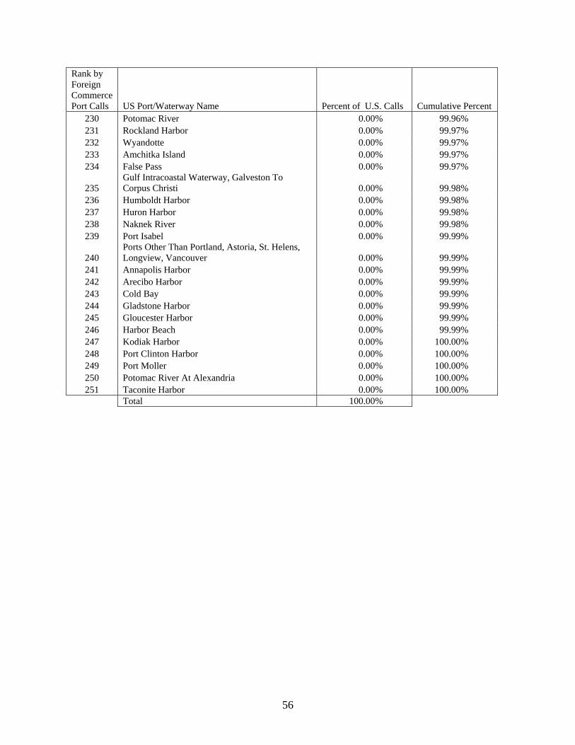
56

Rank by Foreign Commerce Port Calls US Port/Waterway Name Percent of U.S. Calls Cumulative Percent

230 Potomac River 0.00% 99.96% 231 Rockland Harbor 0.00% 99.97% 232 Wyandotte 0.00% 99.97% 233 Amchitka Island 0.00% 99.97% 234 False Pass 0.00% 99.97%

235 Gulf Intracoastal Waterway, Galveston To Corpus Christi 0.00% 99.98%

236 Humboldt Harbor 0.00% 99.98% 237 Huron Harbor 0.00% 99.98% 238 Naknek River 0.00% 99.98% 239 Port Isabel 0.00% 99.99%

240 Ports Other Than Portland, Astoria, St. Helens, Longview, Vancouver 0.00% 99.99%

241 Annapolis Harbor 0.00% 99.99% 242 Arecibo Harbor 0.00% 99.99% 243 Cold Bay 0.00% 99.99% 244 Gladstone Harbor 0.00% 99.99% 245 Gloucester Harbor 0.00% 99.99% 246 Harbor Beach 0.00% 99.99% 247 Kodiak Harbor 0.00% 100.00% 248 Port Clinton Harbor 0.00% 100.00% 249 Port Moller 0.00% 100.00% 250 Potomac River At Alexandria 0.00% 100.00% 251 Taconite Harbor 0.00% 100.00%

Total 100.00%

57

Table A-3. Canadian Port and Waterway Summary from LMIU Movement Data

Rank in LMIU data Canada Ports Percent of Canadian Port Calls Cumulative Percent 1 Vancouver (Canada) 17.54% 17.54% 2 Halifax 12.49% 30.03% 3 Montreal 11.05% 41.08% 4 Quebec 5.23% 46.31% 5 Fraser River Port 3.72% 50.04% 6 Saint John (Canada) 3.26% 53.30% 7 Hamilton (Canada) 3.22% 56.52% 8 Welland Canal 3.12% 59.63% 9 Seven Islands 2.66% 62.29%

10 Point Tupper 2.45% 64.74% 11 Prince Rupert 2.22% 66.96% 12 Port Cartier 1.88% 68.84% 13 Mulgrave 1.75% 70.60% 14 Thunder Bay 1.75% 72.35% 15 Pointe aux Trembles 1.60% 73.95% 16 St. John's (Canada) 1.23% 75.18% 17 Comeau Bay 1.12% 76.31% 18 Sorel 1.05% 77.36% 19 Port Hawkesbury 0.97% 78.32% 20 Three Rivers 0.93% 79.25% 21 Windsor (Canada) 0.86% 80.11% 22 Come by Chance 0.84% 80.94% 23 Toronto 0.80% 81.74% 24 Canso Strait 0.74% 82.48% 25 Port Alfred 0.70% 83.19% 26 Corner Brook 0.69% 83.88% 27 Goderich 0.66% 84.54% 28 Sarnia 0.58% 85.12% 29 Crofton 0.52% 85.63% 30 Nanticoke 0.52% 86.15% 31 Belledune 0.48% 86.63% 32 Victoria (British Columbia) 0.48% 87.11% 33 Port Colborne 0.44% 87.55% 34 Harmac 0.43% 87.98% 35 Clarkson 0.43% 88.40% 36 Contrecoeur 0.40% 88.80% 37 Bayside 0.38% 89.18% 38 Sault Ste. Marie 0.37% 89.55% 39 Charlottetown (Canada) 0.36% 89.91% 40 Dalhousie 0.35% 90.26% 41 Duncan Bay 0.34% 90.60% 42 Becancour 0.33% 90.93% 43 Whiffen Head 0.33% 91.26% 44 Sydney (Nova Scotia) 0.32% 91.58% 45 Cote Ste. Catherine 0.30% 91.88% 46 Meldrum Bay 0.30% 92.18% 47 Corunna (Canada) 0.29% 92.46%

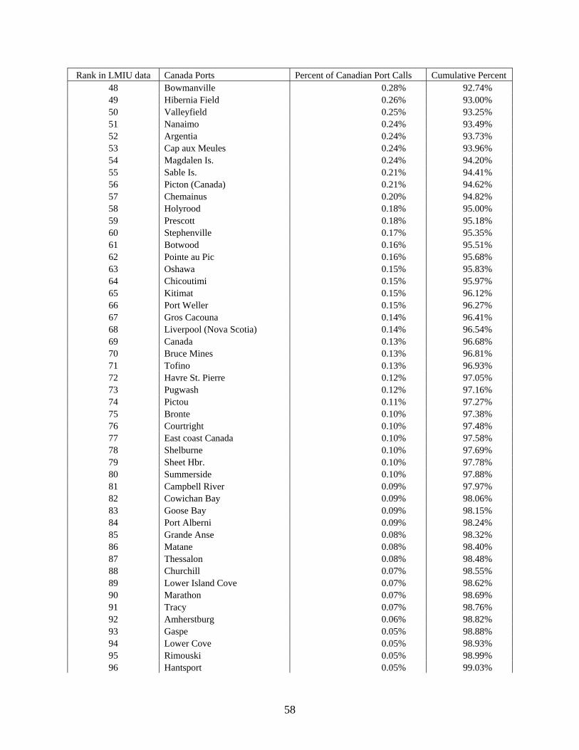
58

Rank in LMIU data Canada Ports Percent of Canadian Port Calls Cumulative Percent 48 Bowmanville 0.28% 92.74% 49 Hibernia Field 0.26% 93.00% 50 Valleyfield 0.25% 93.25% 51 Nanaimo 0.24% 93.49% 52 Argentia 0.24% 93.73% 53 Cap aux Meules 0.24% 93.96% 54 Magdalen Is. 0.24% 94.20% 55 Sable Is. 0.21% 94.41% 56 Picton (Canada) 0.21% 94.62% 57 Chemainus 0.20% 94.82% 58 Holyrood 0.18% 95.00% 59 Prescott 0.18% 95.18% 60 Stephenville 0.17% 95.35% 61 Botwood 0.16% 95.51% 62 Pointe au Pic 0.16% 95.68% 63 Oshawa 0.15% 95.83% 64 Chicoutimi 0.15% 95.97% 65 Kitimat 0.15% 96.12% 66 Port Weller 0.15% 96.27% 67 Gros Cacouna 0.14% 96.41% 68 Liverpool (Nova Scotia) 0.14% 96.54% 69 Canada 0.13% 96.68% 70 Bruce Mines 0.13% 96.81% 71 Tofino 0.13% 96.93% 72 Havre St. Pierre 0.12% 97.05% 73 Pugwash 0.12% 97.16% 74 Pictou 0.11% 97.27% 75 Bronte 0.10% 97.38% 76 Courtright 0.10% 97.48% 77 East coast Canada 0.10% 97.58% 78 Shelburne 0.10% 97.69% 79 Sheet Hbr. 0.10% 97.78% 80 Summerside 0.10% 97.88% 81 Campbell River 0.09% 97.97% 82 Cowichan Bay 0.09% 98.06% 83 Goose Bay 0.09% 98.15% 84 Port Alberni 0.09% 98.24% 85 Grande Anse 0.08% 98.32% 86 Matane 0.08% 98.40% 87 Thessalon 0.08% 98.48% 88 Churchill 0.07% 98.55% 89 Lower Island Cove 0.07% 98.62% 90 Marathon 0.07% 98.69% 91 Tracy 0.07% 98.76% 92 Amherstburg 0.06% 98.82% 93 Gaspe 0.05% 98.88% 94 Lower Cove 0.05% 98.93% 95 Rimouski 0.05% 98.99% 96 Hantsport 0.05% 99.03%

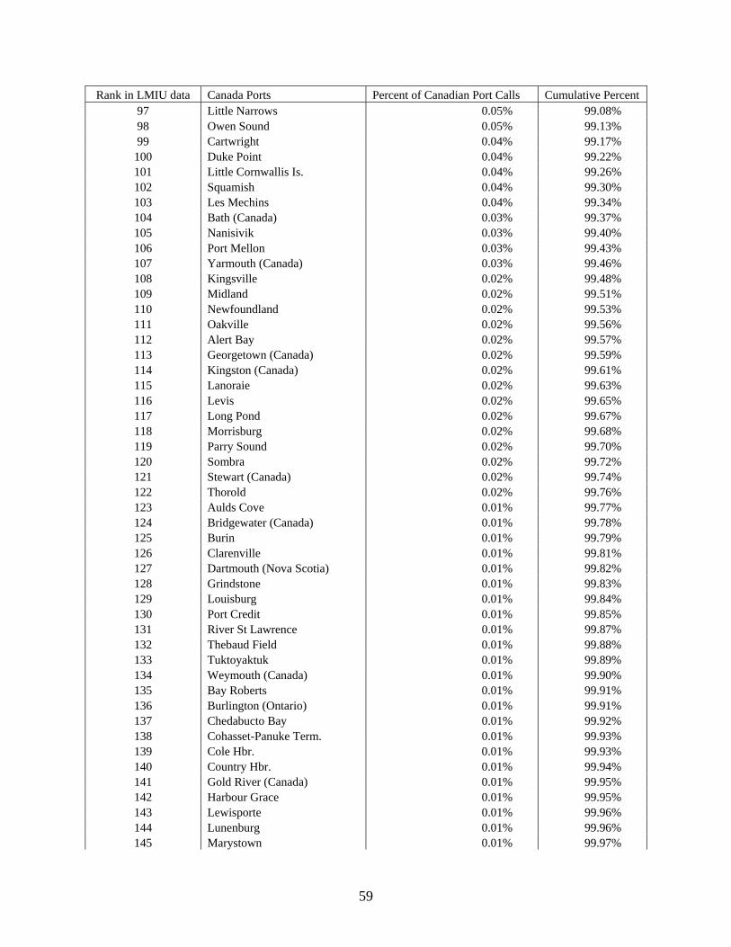
59

Rank in LMIU data Canada Ports Percent of Canadian Port Calls Cumulative Percent 97 Little Narrows 0.05% 99.08% 98 Owen Sound 0.05% 99.13% 99 Cartwright 0.04% 99.17% 100 Duke Point 0.04% 99.22% 101 Little Cornwallis Is. 0.04% 99.26% 102 Squamish 0.04% 99.30% 103 Les Mechins 0.04% 99.34% 104 Bath (Canada) 0.03% 99.37% 105 Nanisivik 0.03% 99.40% 106 Port Mellon 0.03% 99.43% 107 Yarmouth (Canada) 0.03% 99.46% 108 Kingsville 0.02% 99.48% 109 Midland 0.02% 99.51% 110 Newfoundland 0.02% 99.53% 111 Oakville 0.02% 99.56% 112 Alert Bay 0.02% 99.57% 113 Georgetown (Canada) 0.02% 99.59% 114 Kingston (Canada) 0.02% 99.61% 115 Lanoraie 0.02% 99.63% 116 Levis 0.02% 99.65% 117 Long Pond 0.02% 99.67% 118 Morrisburg 0.02% 99.68% 119 Parry Sound 0.02% 99.70% 120 Sombra 0.02% 99.72% 121 Stewart (Canada) 0.02% 99.74% 122 Thorold 0.02% 99.76% 123 Aulds Cove 0.01% 99.77% 124 Bridgewater (Canada) 0.01% 99.78% 125 Burin 0.01% 99.79% 126 Clarenville 0.01% 99.81% 127 Dartmouth (Nova Scotia) 0.01% 99.82% 128 Grindstone 0.01% 99.83% 129 Louisburg 0.01% 99.84% 130 Port Credit 0.01% 99.85% 131 River St Lawrence 0.01% 99.87% 132 Thebaud Field 0.01% 99.88% 133 Tuktoyaktuk 0.01% 99.89% 134 Weymouth (Canada) 0.01% 99.90% 135 Bay Roberts 0.01% 99.91% 136 Burlington (Ontario) 0.01% 99.91% 137 Chedabucto Bay 0.01% 99.92% 138 Cohasset-Panuke Term. 0.01% 99.93% 139 Cole Hbr. 0.01% 99.93% 140 Country Hbr. 0.01% 99.94% 141 Gold River (Canada) 0.01% 99.95% 142 Harbour Grace 0.01% 99.95% 143 Lewisporte 0.01% 99.96% 144 Lunenburg 0.01% 99.96% 145 Marystown 0.01% 99.97%

60

Rank in LMIU data Canada Ports Percent of Canadian Port Calls Cumulative Percent 146 Port Alice 0.01% 99.98% 147 Souris 0.01% 99.98% 148 St. Andrews (Canada) 0.01% 99.99% 149 St. Anthony 0.01% 99.99% 150 Tadoussac 0.01% 100.00%

Total 100.00%

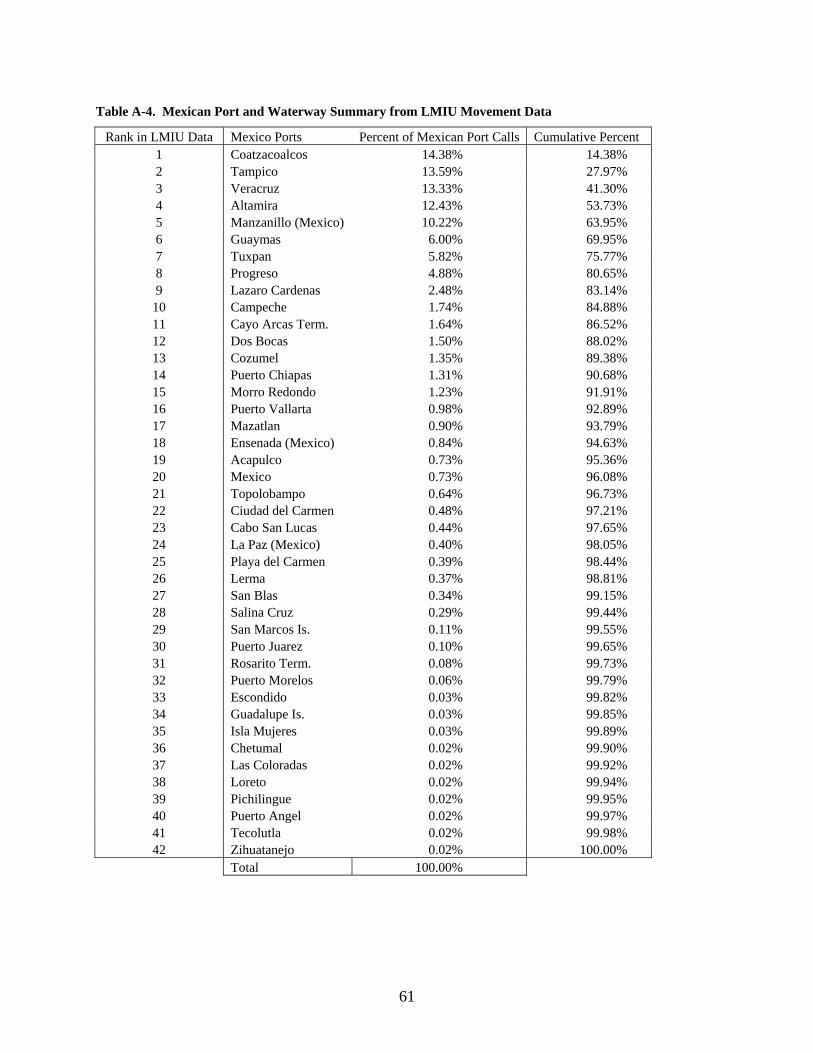
61

Table A-4. Mexican Port and Waterway Summary from LMIU Movement Data

Rank in LMIU Data Mexico Ports Percent of Mexican Port Calls Cumulative Percent 1 Coatzacoalcos 14.38% 14.38% 2 Tampico 13.59% 27.97% 3 Veracruz 13.33% 41.30% 4 Altamira 12.43% 53.73% 5 Manzanillo (Mexico) 10.22% 63.95% 6 Guaymas 6.00% 69.95% 7 Tuxpan 5.82% 75.77% 8 Progreso 4.88% 80.65% 9 Lazaro Cardenas 2.48% 83.14%

10 Campeche 1.74% 84.88% 11 Cayo Arcas Term. 1.64% 86.52% 12 Dos Bocas 1.50% 88.02% 13 Cozumel 1.35% 89.38% 14 Puerto Chiapas 1.31% 90.68% 15 Morro Redondo 1.23% 91.91% 16 Puerto Vallarta 0.98% 92.89% 17 Mazatlan 0.90% 93.79% 18 Ensenada (Mexico) 0.84% 94.63% 19 Acapulco 0.73% 95.36% 20 Mexico 0.73% 96.08% 21 Topolobampo 0.64% 96.73% 22 Ciudad del Carmen 0.48% 97.21% 23 Cabo San Lucas 0.44% 97.65% 24 La Paz (Mexico) 0.40% 98.05% 25 Playa del Carmen 0.39% 98.44% 26 Lerma 0.37% 98.81% 27 San Blas 0.34% 99.15% 28 Salina Cruz 0.29% 99.44% 29 San Marcos Is. 0.11% 99.55% 30 Puerto Juarez 0.10% 99.65% 31 Rosarito Term. 0.08% 99.73% 32 Puerto Morelos 0.06% 99.79% 33 Escondido 0.03% 99.82% 34 Guadalupe Is. 0.03% 99.85% 35 Isla Mujeres 0.03% 99.89% 36 Chetumal 0.02% 99.90% 37 Las Coloradas 0.02% 99.92% 38 Loreto 0.02% 99.94% 39 Pichilingue 0.02% 99.95% 40 Puerto Angel 0.02% 99.97% 41 Tecolutla 0.02% 99.98% 42 Zihuatanejo 0.02% 100.00%

Total 100.00%