estimation of the branching ratio matrix - arxiv.org · june 13, 2017 quantitative finance main to...

June 13, 2017 Quantitative Finance main

To appear in Quantitative Finance, Vol. 00, No. 00, Month 20XX, 1–20

Analysis of order book flows using a nonparametric

estimation of the branching ratio matrix

M. Achab†, E. Bacry†, J. F. Muzy†, ‡ and M. Rambaldi†

†CMAP, Ecole Polytechnique, CNRS, UMR 7641, 91128 Palaiseau, France‡SPE, Universite de Corse, CNRS, UMR 6134, Campus Grimaldi, 20250 Corte, France

(Received 00 Month 20XX; in final form 00 Month 20XX)

We introduce a new non parametric method that allows for a direct, fast and efficient estimation ofthe matrix of kernel norms of a multivariate Hawkes process, also called branching ratio matrix. Wedemonstrate the capabilities of this method by applying it to high-frequency order book data from theEUREX exchange. We show that it is able to uncover (or recover) various relationships between all thefirst level order book events associated with some asset when mapped to a 12-dimensional process. Wethen scale up the model so as to account for events on two assets simultaneously and we discuss the jointhigh-frequency dynamics.

Keywords: Hawkes processes; Non-parametric estimation; GMM method; Order books; MarketMicrostructure;

JEL Classification: C14, C58.

1. Introduction

With the large number of empirical studies devoted to high frequency finance, relying on datasets ofincreasing size and quality, many progresses have been made during the last decade in the modellingand understanding the microstructure of financial markets. Within this context, as evidenced bythis special issue, Hawkes processes have become a very popular class of models. The main reasonis that they allow one to account for the mutual influence of various types of events in a simpleand parsimonious way through a conditional intensity vector. Hawkes processes have been involvedin many different problems of high frequency finance ranging from the simple description of thetemporal occurrence of market orders or price changes (Bowsher (2007), Hardiman and Bouchaud(2014), Filimonov and Sornette (2012)), to the complex modelling of the arrival rates of variouskinds of events in a full order book model (Large (2007), Toke (2011), Jedidi and Abergel (2013)).We refer to Bacry et al. (2015b) for a recent review.

A multivariate Hawkes model of dimension d is characterized by a d×d matrix of kernels, whoseelements φij(t) account for the influence, after a lag t, of events of type j on the arrival rate ofevents of type i. The challenging issue of the statistical estimation of the shape of these excitationkernels has been addressed by many authors and various solutions have been proposed whoseperformances (accuracy and computational complexity) strongly depend on the empirical situationone considers. Indeed, if non-parametric methods like e.g. the EM method (Lewis and Mohler(2011)), the Wiener-Hopf method (Bacry and Muzy (2014), Bacry and Muzy (2016), Bacry et al.(2016)) or the contrast function method (Reynaud-Bouret et al. (2014)) can be applied in lowdimensional situations with a large number of events, one has to consider parametric penalizedalternatives (like e.g., in Zhou et al. (2013a), Yang and Zha (2013)) when one has to handle a system

1

arX

iv:1

706.

0341

1v1

[q-

fin.

TR

] 1

1 Ju

n 20

17


of very large dimension with a relative low number of observed events (as, e.g., when studyingevents associated with the node activities of some social networks).

As far as (ultra) high frequency finance is concerned, the overall number of events can be verylarge. These events occur in a very correlated manner (with long-range correlations) and the systemdimensionality can vary from low to moderately high. In a series of recent papers, Bacry et al.have shown that the non parametric Wiener-Hopf method provides reliable estimations in order todescribe, within a multivariate Hawkes model, various aspects of level-I order book fluctuations: thecoupled dynamics of mid-price changes, market and limit order arrivals (Bacry and Muzy (2014),Bacry et al. (2016)), the impact of market orders (Bacry et al. (2015a)) or the interplay betweenbook orders of different sizes (Rambaldi et al. (2016)). However, if one wants to account for systemsof larger dimensionality by considering for instance a wider class of event types or the book eventsassociated with a basket (e.g. a couple) of assets, then the Wiener-Hopf method (or any othersimilar non-parametric method) may reach its limits as respect to both computational cost andestimation accuracy. On the other hand, a parametric approach can lead to strong bias in theestimated influences between components.

For this reason, in the present paper, we propose to estimate Hawkes models of order book datausing the faster and simpler non-parametric approach introduced in Achab et al. (2016). Thismethod focuses only on the global properties of the Hawkes process. More precisely, it aims atestimating directly the matrix of the kernel norms (also called the branching ratio matrix) withoutpaying attention to the precise shape of these kernels. As recalled in the next section, this matrixdoes not bring all the information about the process dynamics, but is sufficient to disentangle thecomplex interactions between various type of events and estimate the magnitude of their self- andcross- excitations. Moreover, it allows one to estimate the amplitude of fluctuations of endogenousorigin as compared to those of exogenous sources. The method we propose can be considered as themultivariate extension of the approach pioneered by Hardiman and Bouchaud (2014) that proposedto estimate the kernel norm of a one-dimensional Hawkes model directly from the integral of theempirical correlation function. Unfortunately their approach cannot be immediately extended to amultivariate framework because it does not bring a sufficient number of constraints as compared tothe number of unknown parameters. The method of Achab et al. (2016) circumvents this difficultyby taking into account the first three integrated cumulant tensors of Hawkes process.

The paper is organized as follows: in Section 2 we provide the main definitions and propertiesof multivariate Hawkes processes and we introduce the main notations we use all along the paper.The cumulant method of Achab et al. is described and illustrated in Section 3. In Section 4 weestimate the matrix of kernel of Hawkes models for level-I book events associated with 4 differentsvery liquid assets, namely DAX, Euro-Stoxx, Bund and Bobl future contracts. We first consider the8-dimensional model proposed in Bacry et al. (2016) in order to compare our method to the formerresults obtained with a computationally more complex Wiener-Hopf method. We then show thatthe cumulant approach can easily be extended to a 12-dimensional model where all types of level-Ibook events are considered. Within this model, we uncover all the relationships between thesetypes of events and we study the daily amplitude variations of exogenous intensities. In Section5 we investigate the correlation between two assets by considering the events of their order bookwithin a 16-dimensional model. This allows us to discuss the influence of both their tick size andtheir degree of reactivity with respect to the impact of their book events on each other. Section 6contains concluding remarks while some technical details are provided in Appendix.

2. Hawkes processes: definitions and properties

In this section we provide the main definitions and properties of multivariate Hawkes processes andset the notations we need all along the paper.

2


2.1. Multivariate Hawkes processes and the branching ratio matrix G

A multivariate Hawkes process of dimension d is a d-dimensional counting processes N t with aconditional intensity vector λt that is a linear function of past events. More precisely,

λit = µi +

d∑j=1

∫ t

−∞φij(t− s) dN j

s (1)

where µi represents the baseline intensity while the kernel φij(t) quantifies the excitation rate of anevent of type j on the arrival rate of events of type i after a time lag t. In general it is assumedthat each kernel is causal and positive, meaning that Hawkes processes can only account for mutualexcitation effects since the occurrence of some event can only increase the future arrival intensity ofother events. In order to consider the possibility of inhibition effects, one can allow kernels to takenegative values. In that case, we have to consider expression (1) only when it provides a positiveresult while the conditional intensity is assumed to be zero otherwise. Rigorously speaking, suchnon-linear variant of Eq. (1) cannot be handled as simply as the original Hawkes process (Bremaudand Massoulie (1996)) but, as empirically shown in e.g. Reynaud-Bouret et al. (2014) or Bacry andMuzy (2016), if the probability that λit < 0 is small enough, one can safely consider the model aslinear so that all standard expressions provide accurate results. In the following we will suppose thatwe are in this case and we don’t necessarily impose that the kernels φij(t) are positive functions.

Let us define the matrix G as the matrix whose coefficients are the integrals of the kernels φij(t)(that are supported by IR+):

Gij =

∫ +∞

0φij(t)dt . (2)

Let us remark that, as it can directly be seen from the cluster representation of Hawkes processes(Hawkes and Oakes (1974)), Gij represents the mean total number of events of type i directlytriggered by an event of type j. For that reason, in the literature, the matrix G is also referredto as the branching ratio matrix (Hardiman and Bouchaud (2014)). Notice that since the kernelsφij(t) are not necessarily non negative functions, Gij does not in general correspond to the L1 normof φij . For the sake of simplicity, though this is not technically correct, we shall often refer to thematrix G as the “matrix of kernel norms” or more simply the “norm matrix”.

If ‖G‖ stands for the largest eigenvalue of G, it is well known that a sufficient condition for theintensity process λt to be stationary is that ‖G‖ < 1. In the following we will always consider thiscondition satisfied. One can then define the matrix R as:

R = (Id −G)−1, (3)

where Id denotes the identity matrix of dimension d.Let Λ denote the mean intensity vector:

Λ = E(λt) , (4)

so that the ratio µi

Λi represents the fraction of events of type i that are of exogenous origin. One caneasily prove that Λ and µ are related as:

Λ = R µ (5)

If one defines the matrix Ψ as:

Ψ = GR = R− Id, (6)

3


then Ψij represents the average number of events of type i triggered (directly or indirectly) by anexogenous event of type j. When one analyzes empirical data within the framework of Hawkesprocesses, the previous remarks allow one to quantify causal relationships between events in thesense of Granger, i.e., within a well defined mathematical model. In that respect, the coefficientsof the matrices G or Ψ can be read as (Granger-)causality relationships between various types ofevents and used as a tool to disentangle the complexity of the observed flow of events occurring insome experimental situations (Eichler et al. (2017)). Let us emphasize that such causal implicationsare just a matter of interpretation of data within a specific model (namely a Hawkes model) andshould simply be considered as a convenient and parsimonious way to represent that data. Theyshould not, in any way, be understood as a “physical” causality reflecting their “real nature”.

2.2. Integrated Cumulants of Hawkes Process

The NPHC algorithm developed in Achab et al. (2016) and described in Sec. 3 below, enables thedirect estimation of the matrix G from a single or several realizations of the process. It relies onthe computation of low order cumulant functions whose expressions are recalled below.

Given 1 ≤ i, j, k ≤ d, the first three integrated cumulants of the Hawkes process can be, thanksto stationarity, defined as follows:

Λidt = E(dN it ) (7)

Cijdt =

∫τ∈R

(E(dN i

tdNjt+τ )− E(dN i

t )E(dN jt+τ )

)(8)

Kijkdt =

∫ ∫τ,τ ′∈R2

(E(dN i

tdNjt+τdN

kt+τ ′) + 2E(dN i

t )E(dN jt+τ )E(dNk

t+τ ′)

− E(dN itdN

jt+τ )E(dNk

t+τ ′)− E(dN itdN

kt+τ ′)E(dN j

t+τ )− E(dN jt+τdN

kt+τ ′)E(dN i

t )),

(9)

where Eq. (7) is the mean intensity of the Hawkes process, the second-order cumulant (8) refers tothe integrated covariance density matrix and the third-order cumulant (9) measures the skewnessof N t. Using the martingale representation (Bacry and Muzy (2016)) or the Poisson cluster processrepresentation (Jovanovic et al. (2015)), one can obtain an explicit relationship between theseintegrated cumulants and the matrix R (and therefore the matrix G thanks to Eq. (3)). Somestraightforward computations (see Achab et al. (2016)) lead to the following identities:

Λi =

d∑m=1

Rimµm (10)

Cij =

d∑m=1

ΛmRimRjm (11)

Kijk =

d∑m=1

(RimRjmCkm +RimCjmRkm + CimRjmRkm − 2ΛmRimRjmRkm). (12)

3. The NPHC method

In this section we briefly recall the main lines of the recent non parametric method proposed inAchab et al. (2016) that leads to a fast and robust direct estimation of the branching ratio matrix

4


G without estimating the shape of the kernel functions. This method is based on the remark that,as shown in Jovanovic et al. (2015) and as it can be seen in Eqs. (10), (11) and (12), the integratedcumulants of a Hawkes process can be explicitly written as functions of R. The NPHC method is amoment method that consists in directly exploiting these equations to recover R and thus G.

3.1. Estimation of the integrated cumulants

Let us first introduce explicit formulas to estimate the three moment-based quantities listed in theprevious section, namely, Λ, C and K. In what follows, we assume there exists H > 0 such that thetruncation from (−∞,+∞) to [−H,H] of the domain of integration of the quantities appearingin Eqs. (8) and (9) introduces only a small error. This amounts to neglecting tail effects in thecovariance density and in the skewness density, and it corresponds to a good approximation if(i) each kernel φij(t) is essentially supported by [0, H] and (ii) the spectral norm ‖G‖ is less than 1.In this case, given a realization of a stationary Hawkes process {N t : t ∈ [0, T ]}, as shown in Achabet al. (2016), we can write the estimators of the first three cumulants (7), (8) and (9) as

Λi =1

T

∑τ∈Zi

1 =N iT

T(13)

Cij =1

T

∑τ∈Zi

(N jτ+H −N

jτ−H − 2HΛj

)(14)

Kijk =1

T

∑τ∈Zi

(N jτ+H −N

jτ−H − 2HΛj

)·(Nkτ+H −Nk

τ−H − 2HΛk)

− Λi

T

∑τ∈Zj

∑τ ′∈Zk

(2H − |τ ′ − τ |)+ + 4H2ΛiΛjΛk.

(15)

In practice, the filtering parameter H is selected by (i) computing estimates of the covariancedensity at several points t 1, (ii) assessing the characteristic time τc after which the covariancedensity is negligible, and (iii) setting a multiple of τc for H, for instance H = 5τc.

3.2. The NPHC algorithm

The covariance C only provides d(d+ 1)/2 independent coefficients and is therefore not sufficientto uniquely identify the d2 coefficients of the matrix G. In order to set a sufficient number ofconstraints, the NPHC approach relies on using all the covariance C along with a restricted numberof the (d3 + 3d2 + 2d)/6 third-order independent cumulant components, namely the d2 coefficients

Kc = {Kiij}1≤i,j≤d. Thus, we define the estimator of R as R ∈ argminRL(R), where

L(R) = (1− κ)‖Kc(R)− Kc‖22 + κ‖C(R)− C‖22, (16)

where ‖ · ‖2 stands for the Frobenius norm, while Kc and C are the respective estimators of Cand Kc as defined in Equations (14), (15) above. It is noteworthy that the above mean squareerror approach can be seen as a peculiar instance of Generalized Method of Moments (GMM),see Hall (2005), Hansen (1982). Though this framework allows to determine the optimal weightingmatrix involved in the loss function, in practice this approach is unusable, as the associatedcomplexity is too high. Indeed, since we have d2 parameters, this matrix has d4 coefficients and

1the pointwise covariance density at t can be estimated with 1hT

∑τ∈Zi

(Njτ+t+h −N

jτ+t − hΛj

)for a small h

5


t

φt

0 γ γ + 1/β

αβ

(a) Rectangular kernel

log t

log φt

− log β

logαβγ

slope ≈ −(1 + γ)

(b) Power-law kernel on log-log scale

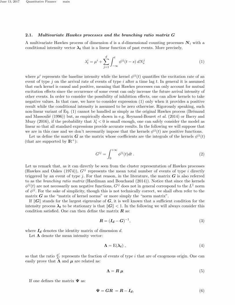
Figure 1. The two different kernels used to simulate the datasets.

GMM calls for computing its inverse leading to a O(d6) complexity. Thus, instead, we choose touse the loss function (16) in which, so as to be of the same order, the two terms are rescaled using

κ = ‖Kc‖22/(‖Kc‖22 + ‖C‖22). We refer to Appendix A for an explanation of how κ is related to theweighting matrix. Finally the estimator of G is straightforwardly obtained as

G = Id − R−1,

from the inversion of Eq. (2). The authors of Achab et al. (2016) proved the consistency of the

so-obtained estimator G, i.e. the convergence in probability to the true value, when the observationtime T goes to infinity.

Let us mention that, when applied to financial time-series, the number of events is generally largeas compared with d (i.e., n = maxi |Zi| � d), thus the matrix inversion in the previous formula isnot the bottleneck of the algorithm. Indeed, it has a complexity O(d3) which is cheap as comparedwith the computation of the cumulants which is O(nd2). Thus, assuming the loss function (16) isminimized after Niter iterations, the overall complexity of the algorithm is O(nd2 +Niterd

3). Theauthors of Achab et al. (2016) compared the complexity of their algorithm with other state-of-the-artmethods’ ones, namely the ordinary differential equations based (ODE) algorithm in Zhou et al.(2013b), the Sum of Gaussians based algorithm in Xu et al. (2016), the ADM4 algorithm in Zhouet al. (2013a), and the Wiener-Hopf-based algorithm in Bacry and Muzy (2016). The complexity ofNPHC is smaller, because the algorithm NPHC directly estimates the kernels’ integrals while othermethods go through the estimation of the kernel functions themselves.

3.3. Numerical experiments

As mentioned above, the NPHC algorithm is non parametric and provides an estimation of theintegral of the kernels regardless of their shapes. In order to illustrate the stability of our methodwith respect to the shape of the kernels, we simulated two datasets with Ogata’s Thinning algorithmintroduced in Ogata (1981) using the open-source library tick1. Each dataset corresponds to adifferent kernel shape (but with the same norm), a rectangular kernel and a power-law kernel, bothrepresented in Figure 1:

rectangular kernel: φ(t) = αβ1[0,1/β](t− γ) (17)

power law kernel: φ(t) = αβγ(1 + βt)−(1+γ) (18)

1https://github.com/X-DataInitiative/tick

6

https://github.com/X-DataInitiative/tick


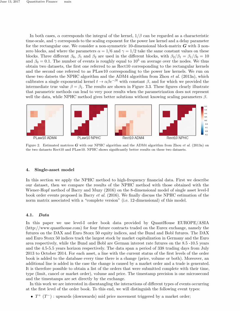
In both cases, α corresponds the integral of the kernel, 1/β can be regarded as a characteristictime-scale, and γ corresponds to the scaling exponent for the power law kernel and a delay parameterfor the rectangular one. We consider a non-symmetric 10-dimensional block-matrix G with 3 non-zero blocks, and where the parameters α = 1/6 and γ = 1/2 take the same constant values on theseblocks. Three different β0, β1 and β2 are used in the different blocks, with β2/β1 = β1/β0 = 10and β0 = 0.1. The number of events is roughly equal to 105 on average over the nodes. We thusobtain two datasets, the first one referred to as Rect10 corresponding to the rectangular kernelsand the second one referred to as PLaw10 corresponding to the power law kernels. We run onthese two datsets the NPHC algorithm and the ADM4 algorithm from Zhou et al. (2013a), whichcalibrates a single exponential kernel t→ αβe−βt with constant β, and for which we provided theintermediate true value β = β1. The results are shown in Figure 3.3. These figures clearly illustratethat parametric methods can lead to very poor results when the parametrization does not representwell the data, while NPHC method gives better solutions without knowing scaling parameters β.

Figure 2. Estimated matrices G with our NPHC algorithm and the ADM4 algorithm from Zhou et al. (2013a) onthe two datasets Rect10 and PLaw10. NPHC shows significantly better results on these two datasets.

4. Single-asset model

In this section we apply the NPHC method to high-frequency financial data. First we describeour dataset, then we compare the results of the NPHC method with those obtained with theWiener-Hopf method of Bacry and Muzy (2016) on the 8-dimensional model of single asset level-Ibook order events proposed in Bacry et al. (2016). We finally discuss the NPHC estimation of thenorm matrix associated with a “complete version” (i.e. 12-dimensional) of this model.

4.1. Data

In this paper we use level-I order book data provided by QuantHouse EUROPE/ASIA(http://www.quanthouse.com) for four future contracts traded on the Eurex exchange, namely thefutures on the DAX and Euro Stoxx 50 equity indices, and the Bund and Bobl futures. The DAXand Euro Stoxx 50 indices track the largest stock by market capitalization in Germany and the Euroarea respectively, while the Bund and Bobl are German interest rate futures on the 8.5 -10.5 yearsand the 4.5-5.5 years horizon respectively. The data span a period of 338 trading days from July2013 to October 2014. For each asset, a line with the current status of the first levels of the orderbook is added to the database every time there is a change (price, volume or both). Moreover, anadditional line is added in the case the change is caused by a market order and a trade is generated.It is therefore possible to obtain a list of the orders that were submitted complete with their time,type (limit, cancel or market order), volume and price. The timestamp precision is one microsecondand the timestamps are set directly by the exchange.

In this work we are interested in disentangling the interactions of different types of events occurringat the first level of the order book. To this end, we will distinguish the following event types:

• T+ (T−) : upwards (downwards) mid price movement triggered by a market order;

7


T+ T− L+ L− C+ C− T a T b La Lb Ca Cb

DAX 11.9 11.9 21.8 21.9 10.1 10.1 11.6 11.7 80.0 79.5 97.3 96.1ESXX 2.6 2.6 3.5 3.6 0.9 0.9 16.4 16.5 176.0 174.7 172.4 170.8Bund 3.2 3.2 4.0 4.0 0.8 0.8 14.5 14.7 125.4 125.0 111.5 110.7Bobl 1.1 1.1 1.5 1.5 0.5 0.5 6.1 6.1 86.5 86.8 81.6 81.4

Table 1. Average number of events in thousands per type in a trading day (from open at 08:00 to closing at 22:00Frankfurt time) for the four assets considered.

• L+ (L−) : upwards (downwards) mid price movement triggered by a limit order;• C+ (C−) : upwards (downwards) mid price movement triggered by a cancel order;• T a (T b) : market order at the ask (bid) that does not move the mid price;• La (Lb) : limit order at the ask (bid) that does not move the mid price;• Ca (Cb) : cancellation order at the ask (bid) that does not move the mid price.

Additionally, we introduce the symbols P+ (P−) to denote an upwards (downwards) mid pricemovement irrespectively of its origin. In Table 1 we report the average number of events per day(from 08:00 am to 10:00 pm) for each asset and each type. We remark that all four assets areextremely active securities with an average of more than 300.000 events per day.

One characteristic that strongly influences the order book dynamics at short time scales is thetick size to average spread ratio. When this ratio is close to one (resp. much smaller than one), theasset is said to be a “large tick asset” (resp. a “small tick asset”) (see, e.g., Dayri and Rosenbaum(2015)). In our dataset, all assets are large-tick assets (the spread is equal to one tick in more than95% of the times) except for the DAX future, which is a small-tick one. As evidenced by Table 1,the price changes much less frequently on large tick assets. One can also remark that the quantityavailable at the best quotes tends do be proportionally much larger on large tick assets. Thesemicrostructural characteristics will be reflected by our analysis.

4.2. Revising the 8-dimensional mono-asset model of Bacry et al. (2016) : Asanity check

In Bacry and Muzy (2014), Bacry and Muzy (2016), the authors outlined a method for non-parametric estimation of the Hawkes kernel functions based the infinitesimal covariance densityand the numerical solution of a Wiener-Hopf system of integral equations that links the covariancematrix and the kernel matrix. Their method has been applied to high-frequency financial data inBacry and Muzy (2014), Bacry et al. (2016), and Rambaldi et al. (2016).

The aim of this section is to compare the newly proposed NPHC methodology with the Wiener-Hopf method mentioned above in order to assess the reliability of the new NPHC method. To thisend, we reproduce the results obtained in Bacry et al. (2016).

As it was done there, we consider the DAX and Bund futures data1 and for each asset we separateLevel-I order book events into 8 categories as defined above: P+, P−, T a, T b, La, Lb, and Ca,Cb. Note that here a price move can be of any type. We then consider the timestamp associatedwith all events as a realization of a 8-dimensional Hawkes process and we use both the NPHCmethod outlined in Section 3 and the Wiener-Hopf method of Bacry and Muzy (2016) to estimatethe integrated kernel interaction matrix G from the data. For the Wiener-Hopf method, we followthe same procedure as Bacry et al. (2016) and in particular we estimate the covariance densityup to a maximum lag of ≈ 1000s using a log-linear spaced grid2, while for the NPHC method wefollow the steps outlined in Section 3 and we fix H = 500s so to be on a comparable scale with

1Note that we use the very same dataset as in Bacry et al. (2016)2As was done in Bacry et al. (2016), for the estimation of the covariance density we take a linearly spaced grid at short time lags

(until a lag of 1ms) and we switch to a log-spaced one for longer time lags. This allows to estimate the covariance on severalorders of magnitude in time.

8


P + P − T a T b L a L b C a C b

Cb

Ca

Lb

La

Tb

Ta

P−

P+

0.8

0.4

0.0

0.4

0.8

P + P − T a T b L a L b C a C b

Cb

Ca

Lb

La

Tb

Ta

P−

P+

0.8

0.4

0.0

0.4

0.8

Figure 3. Kernel norm matrix G estimated with the NPHC method for the DAX future (left) and with the Wiener-Hopf method of Bacry and Muzy (2016) (right) when the 8-dimensional model described in Section 4.2 is considered.

the Wiener-Hopf method. Let us note that this scale is several orders of magnitude larger than thetypical inter-event time. Indeed, on the assets considered median inter-event times are of the orderof 300µs (the mean being ≈ 50ms), with minimum time distances in the tens of microseconds.

In Figure 3, we compare the kernel integral matrices G obtained with the NPHC method (left)with those obtained with the Wiener-Hopf approach (right) on the DAX future. Although the precisevalues of the matrix entries differ somewhat, as it is difficult to tune the estimation parameters ofthe two methods as to produce the exact same numerical results, we note that the two methodsproduce very consistent results. Indeed, they recover the same interaction structure and thus leadto the same interpretation of the underlying system dynamics. In our view, this represents a goodsanity check for the proposed NPHC methodology. Analogous results are obtained for the Bundfuture. Let us also point out that the small asymmetries between symmetric interactions (such ase.g. T+ → T− and T− → T+) can be used get a rough measure of the estimation error. In thecase presented here, the average absolute difference between symmetric interactions kernels is 0.03,which means relative error of a few percent on the most relevant interactions.

We do not comment here the features emerging from the kernel norm matrices presented in thissection since they have been already discussed at length in (Bacry et al. 2016) and some of themwill be further discussed in the next sections. Instead, here we highlight that the results of thissection provide a strong case for the use of the NPHC method over the Wiener-Hopf method whenthe focus is solely on the kernel interaction matrix. Indeed, in order to estimate the kernel normmatrix with the Wiener-Hopf method, the full kernel functions have to be estimated first and thennumerically integrated. The NPHC method thus represents a much faster alternative, as it does notrequire the estimation of d2 functions but directly estimates their integrals. Besides the speed gain,the gain in complexity allows NPHC to scale much better when increasing the dimension, i.e., whenusing more detailed models.

4.3. A 12-dimensional mono-asset model

By estimating directly the norm of the kernels and not the whole kernel function, the NPHC methodcan be used to investigate systems of greater dimension. In this section we extend the model ofSection 4.2 to 12 dimensions by separating the type of events that lead to a price move. The 12even types we consider are thus T+ (T−), L+ (L−), C+ (C−), T a (T b), La (Lb), Ca (Cb). We thenapply the NPHC algorithm to estimate the branching ratio matrix. When not otherwise specified,we set H = 500s. To further assess the validity of our methodology and the impact of time-of-dayeffects, we first estimate the model using different time slots within the trading day. In Section 4.3.2

9


T + T − L + L − C + C − T a T b L a L b C a C b

CbCaLbLaTbTaC−C

+L−L

+T−T

+

08:00 - 10:00

0.6

0.3

0.0

0.3

0.6


CbCaLbLaTbTaC−C

+L−L

+T−T

+

12:00 - 14:00

0.6

0.3

0.0

0.3

0.6


CbCaLbLaTbTaC−C

+L−L

+T−T

+

16:00 - 18:00

0.6

0.3

0.0

0.3

0.6

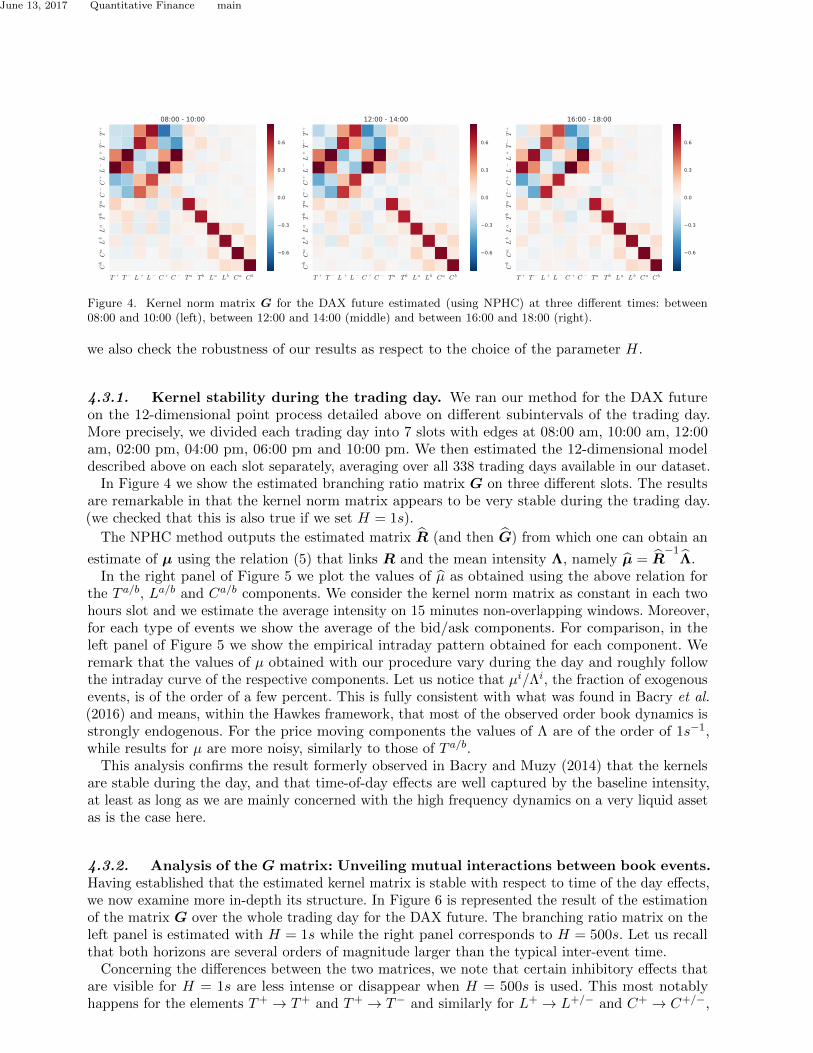
Figure 4. Kernel norm matrix G for the DAX future estimated (using NPHC) at three different times: between08:00 and 10:00 (left), between 12:00 and 14:00 (middle) and between 16:00 and 18:00 (right).

we also check the robustness of our results as respect to the choice of the parameter H.

4.3.1. Kernel stability during the trading day. We ran our method for the DAX futureon the 12-dimensional point process detailed above on different subintervals of the trading day.More precisely, we divided each trading day into 7 slots with edges at 08:00 am, 10:00 am, 12:00am, 02:00 pm, 04:00 pm, 06:00 pm and 10:00 pm. We then estimated the 12-dimensional modeldescribed above on each slot separately, averaging over all 338 trading days available in our dataset.

In Figure 4 we show the estimated branching ratio matrix G on three different slots. The resultsare remarkable in that the kernel norm matrix appears to be very stable during the trading day.(we checked that this is also true if we set H = 1s).

The NPHC method outputs the estimated matrix R (and then G) from which one can obtain an

estimate of µ using the relation (5) that links R and the mean intensity Λ, namely µ = R−1

Λ.In the right panel of Figure 5 we plot the values of µ as obtained using the above relation for

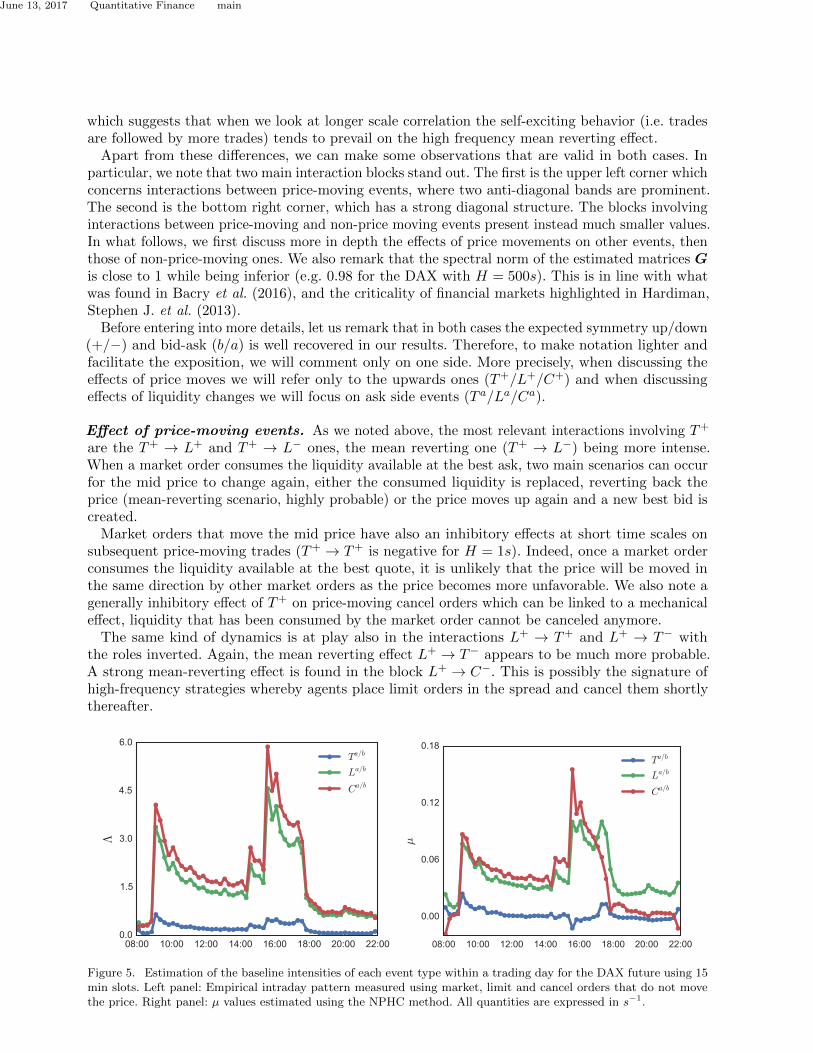
the T a/b, La/b and Ca/b components. We consider the kernel norm matrix as constant in each twohours slot and we estimate the average intensity on 15 minutes non-overlapping windows. Moreover,for each type of events we show the average of the bid/ask components. For comparison, in theleft panel of Figure 5 we show the empirical intraday pattern obtained for each component. Weremark that the values of µ obtained with our procedure vary during the day and roughly followthe intraday curve of the respective components. Let us notice that µi/Λi, the fraction of exogenousevents, is of the order of a few percent. This is fully consistent with what was found in Bacry et al.(2016) and means, within the Hawkes framework, that most of the observed order book dynamics isstrongly endogenous. For the price moving components the values of Λ are of the order of 1s−1,while results for µ are more noisy, similarly to those of T a/b.

This analysis confirms the result formerly observed in Bacry and Muzy (2014) that the kernelsare stable during the day, and that time-of-day effects are well captured by the baseline intensity,at least as long as we are mainly concerned with the high frequency dynamics on a very liquid assetas is the case here.

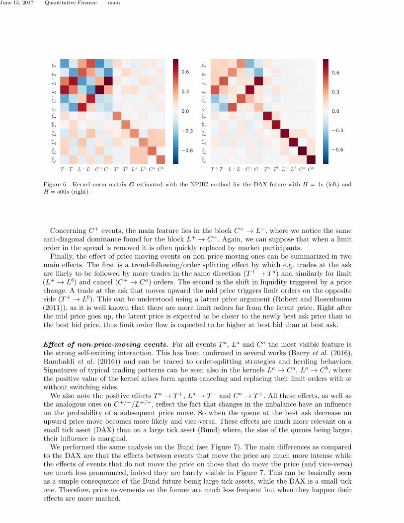
4.3.2. Analysis of the G matrix: Unveiling mutual interactions between book events.Having established that the estimated kernel matrix is stable with respect to time of the day effects,we now examine more in-depth its structure. In Figure 6 is represented the result of the estimationof the matrix G over the whole trading day for the DAX future. The branching ratio matrix on theleft panel is estimated with H = 1s while the right panel corresponds to H = 500s. Let us recallthat both horizons are several orders of magnitude larger than the typical inter-event time.

Concerning the differences between the two matrices, we note that certain inhibitory effects thatare visible for H = 1s are less intense or disappear when H = 500s is used. This most notablyhappens for the elements T+ → T+ and T+ → T− and similarly for L+ → L+/− and C+ → C+/−,

10


which suggests that when we look at longer scale correlation the self-exciting behavior (i.e. tradesare followed by more trades) tends to prevail on the high frequency mean reverting effect.

Apart from these differences, we can make some observations that are valid in both cases. Inparticular, we note that two main interaction blocks stand out. The first is the upper left corner whichconcerns interactions between price-moving events, where two anti-diagonal bands are prominent.The second is the bottom right corner, which has a strong diagonal structure. The blocks involvinginteractions between price-moving and non-price moving events present instead much smaller values.In what follows, we first discuss more in depth the effects of price movements on other events, thenthose of non-price-moving ones. We also remark that the spectral norm of the estimated matrices Gis close to 1 while being inferior (e.g. 0.98 for the DAX with H = 500s). This is in line with whatwas found in Bacry et al. (2016), and the criticality of financial markets highlighted in Hardiman,Stephen J. et al. (2013).

Before entering into more details, let us remark that in both cases the expected symmetry up/down(+/−) and bid-ask (b/a) is well recovered in our results. Therefore, to make notation lighter andfacilitate the exposition, we will comment only on one side. More precisely, when discussing theeffects of price moves we will refer only to the upwards ones (T+/L+/C+) and when discussingeffects of liquidity changes we will focus on ask side events (T a/La/Ca).

Effect of price-moving events. As we noted above, the most relevant interactions involving T+

are the T+ → L+ and T+ → L− ones, the mean reverting one (T+ → L−) being more intense.When a market order consumes the liquidity available at the best ask, two main scenarios can occurfor the mid price to change again, either the consumed liquidity is replaced, reverting back theprice (mean-reverting scenario, highly probable) or the price moves up again and a new best bid iscreated.

Market orders that move the mid price have also an inhibitory effects at short time scales onsubsequent price-moving trades (T+ → T+ is negative for H = 1s). Indeed, once a market orderconsumes the liquidity available at the best quote, it is unlikely that the price will be moved inthe same direction by other market orders as the price becomes more unfavorable. We also note agenerally inhibitory effect of T+ on price-moving cancel orders which can be linked to a mechanicaleffect, liquidity that has been consumed by the market order cannot be canceled anymore.

The same kind of dynamics is at play also in the interactions L+ → T+ and L+ → T− withthe roles inverted. Again, the mean reverting effect L+ → T− appears to be much more probable.A strong mean-reverting effect is found in the block L+ → C−. This is possibly the signature ofhigh-frequency strategies whereby agents place limit orders in the spread and cancel them shortlythereafter.

08:00 10:00 12:00 14:00 16:00 18:00 20:00 22:000.0

1.5

3.0

4.5

6.0

Λ

Ta/b

La/b

Ca/b

08:00 10:00 12:00 14:00 16:00 18:00 20:00 22:00

0.00

0.06

0.12

0.18

µ

Ta/b

La/b

Ca/b

Figure 5. Estimation of the baseline intensities of each event type within a trading day for the DAX future using 15min slots. Left panel: Empirical intraday pattern measured using market, limit and cancel orders that do not movethe price. Right panel: µ values estimated using the NPHC method. All quantities are expressed in s−1.

11


T + T − L + L − C +C − T a T b L a L b C a C b

CbCaLbLaTbTaC−C

+L−L

+T−T

+

0.6

0.3

0.0

0.3

0.6


CbCaLbLaTbTaC−C

+L−L

+T−T

+

0.6

0.3

0.0

0.3

0.6

Figure 6. Kernel norm matrix G estimated with the NPHC method for the DAX future with H = 1s (left) andH = 500s (right).

Concerning C+ events, the main feature lies in the block C+ → L−, where we notice the sameanti-diagonal dominance found for the block L+ → C−. Again, we can suppose that when a limitorder in the spread is removed it is often quickly replaced by market participants.

Finally, the effect of price moving events on non-price moving ones can be summarized in twomain effects. The first is a trend-following/order splitting effect by which e.g. trades at the askare likely to be followed by more trades in the same direction (T+ → T a) and similarly for limit(L+ → Lb) and cancel (C+ → Ca) orders. The second is the shift in liquidity triggered by a pricechange. A trade at the ask that moves upward the mid price triggers limit orders on the oppositeside (T+ → Lb). This can be understood using a latent price argument (Robert and Rosenbaum(2011)), as it is well known that there are more limit orders far from the latent price. Right afterthe mid price goes up, the latent price is expected to be closer to the newly best ask price than tothe best bid price, thus limit order flow is expected to be higher at best bid than at best ask.

Effect of non-price-moving events. For all events T a, La and Ca the most visible feature isthe strong self-exciting interaction. This has been confirmed in several works (Bacry et al. (2016),Rambaldi et al. (2016)) and can be traced to order-splitting strategies and herding behaviors.Signatures of typical trading patterns can be seen also in the kernels La → Ca, La → Cb, wherethe positive value of the kernel arises form agents canceling and replacing their limit orders with orwithout switching sides.

We also note the positive effects T a → T+, La → T− and Ca → T+. All these effects, as well asthe analogous ones on C+/−/L+/−, reflect the fact that changes in the imbalance have an influenceon the probability of a subsequent price move. So when the queue at the best ask decrease anupward price move becomes more likely and vice-versa. These effects are much more relevant on asmall tick asset (DAX) than on a large tick asset (Bund) where, the size of the queues being larger,their influence is marginal.

We performed the same analysis on the Bund (see Figure 7). The main differences as comparedto the DAX are that the effects between events that move the price are much more intense whilethe effects of events that do not move the price on those that do move the price (and vice-versa)are much less pronounced, indeed they are barely visible in Figure 7. This can be basically seenas a simple consequence of the Bund future being large tick assets, while the DAX is a small tickone. Therefore, price movements on the former are much less frequent but when they happen theireffects are more marked.

12



CbCaLbLaTbTaC−C

+L−L

+T−T

+

1.2

0.6

0.0

0.6

1.2


CbCaLbLaTbTaC−C

+L−L

+T−T

+

1.6

0.8

0.0

0.8

1.6

Figure 7. Kernel norm matrix G estimated with the NPHC method for the Bund future with H = 1s (left) andH = 500s (right).

4.3.3. Analysis of the Ψ matrix: the fingerprint of meta-orders. As discussed in Sec-tion 2, the elements of the matrix Ψ quantifies the total effect, direct and indirect, of an eventof type j on events of type i. More precisely, thanks to the branching process structure, we caninterpret ψij as the mean number of events of type i generated by a single exogenous ancestor oftype j. We plot the estimated matrices Ψ for the DAX and Bund futures in Figure 8. The mainfeature that appears for both assets is the set of strong values found in the bottom right corner,namely in the columns and lines associated with La/b and Ca/b. We note that an exogenous limitor cancel event generates a large number of limit and cancel events and, to a lesser extent, tradeevents. This can be read as the signature of meta-orders. Indeed, if an agent wants to sell a largenumber of contracts1, he will place a meta-order, i.e., he will optimize the overall cost by dividingthis large order into several smaller orders. The overall optimization will result in many limit/cancelsell orders La, Ca and, as less as possible, of sell market orders T b (the cost of a market order is onaverage higher than that of a limit order). The same description can be applied to understand whyan exogenous sell market order T b generates mainly limit and cancel sell orders La, Ca as well asother sell market orders T b.

Due to the much lower values of the exogenous intensities for price moving events, the left part ofthe Ψ matrix is more noisy. Nevertheless, at least in the DAX case, we note also for the price movingcomponents the prevalence of the L+ → L+ and L+ → C− elements, which are the price-movingcounterparts of the effect described for La.

Finally, we also remark that although we noted several inhibition effects in the matrices G, theelements of Ψ are non negative. This suggests that most inhibition effects are short lived and theeffect of an event arrival is towards an increase of the overall intensity. This is in line with what wasfound in Bacry et al. (2016) and Rambaldi et al. (2016), where the inhibitions effects were shownto be mostly concentrated around the typical market reaction time.

Within the branching ratio representation of Hawkes processes, µj

Λiψij represents the fraction ofevents of type i that has a type j as primary ancestor. Along the same line, we can estimate thefraction of aggressive orders (i.e. all T ), as opposed to passive orders (L or C), that is ultimately

1Let us recall that, in our discussion, we only address half of the matrix coefficients since the discussion on the other half can be

obtained using the symmetries ask/bid, buy/sell, price up/price down. Following these lines, we only consider here the case of aselling meta-order.

13



CbCaLbLaTbTaC−C

+L−L

+T−T

+

0

4

8

12

16

20


CbCaLbLaTbTaC−C

+L−L

+T−T

+

0

5

10

15

20

Figure 8. Ψ matrix of eq. (6) estimated with the NPHC method for the DAX future (left) and the Bund future(right) with H = 500s.

generated by another aggressive order, as:

1∑i={T+/−,T a/b} Λi

∑j={T+/−,T a/b}

∑i={T+/−,T a/b}

ψijµj . (19)

We find that for both assets this fraction is about 10%, which means that the large majority ofmarket orders have a “passive order” (L or C) oldest ancestor. We compute the analogous fractionfor passive orders and we find that for both assets more than 96% of the passive orders (L or C)have an oldest ancestor that is itself a passive (L or C) order. This fact is in line with the idea thatmeta-orders would be at the origin of most of the trading activity within the order book.

5. Multi-asset model

Studying and quantifying the interactions and comovements within a basket of assets is an importanttopic in finance. Most of these studies focus on the return correlations properties in relationship withportfolio theory. At very high frequency, the discrete nature of price variations and the asynchronousoccurrence of price change events make the correlation analysis trickier and, in order to avoid wellknown bias (like the Epps effect) one has to use specific techniques like the estimator proposed byHayashi et al. (2005). Hawkes processes, being naturally defined in continuous time, can representa complementary tool for the investigation of high-frequency cross-asset dynamics.

The idea of capturing the joint dynamic of multiple assets via Hawkes processes has only beenconsidered in few recent papers. Let us mention the work proposed by Bormetti et al. (2015) whichmodels the simultaneous cojumps of different assets using a one-dimensional Hawkes process, and amore recent work (Da Fonseca and Zaatour (2017)) which focuses on the correlation and lead-lagrelationships between the price changes of two assets, in the spirit of Bacry et al. (2013).

In this section, we aim at unveiling a more precise structure of the high-frequency cross-assetdynamics by pushing further the dimensionality of the model to include simultaneously events ontwo assets. We first consider the pair DAX-EURO STOXX and then the one Bobl-Bund. The pairsof assets considered here are tightly related, as they share exposure to the same risk factors and, inthe case of DAX-EURO STOXX, also because the underlying indices actually share a significantpart of their components. This is confirmed also by Table 2 where we report 5 minutes returncorrelations among the considered assets.

In this section we consider the same kind of events as in Section 4.2 and we have therefore a

14


16-dimensional model (2× 8) corresponding to 256 possible interactions. Let us point out that thisis quite a large dimension value for a non parametric methodology.

DAX ESXX Bobl Bund

DAX 1.00 0.89 -0.18 -0.22ESXX 0.89 1.00 -0.19 -0.22Bobl -0.18 -0.19 1.00 0.85Bund -0.22 -0.22 0.85 1.00

Table 2. Five minutes return correlation coefficients for the examined assets.

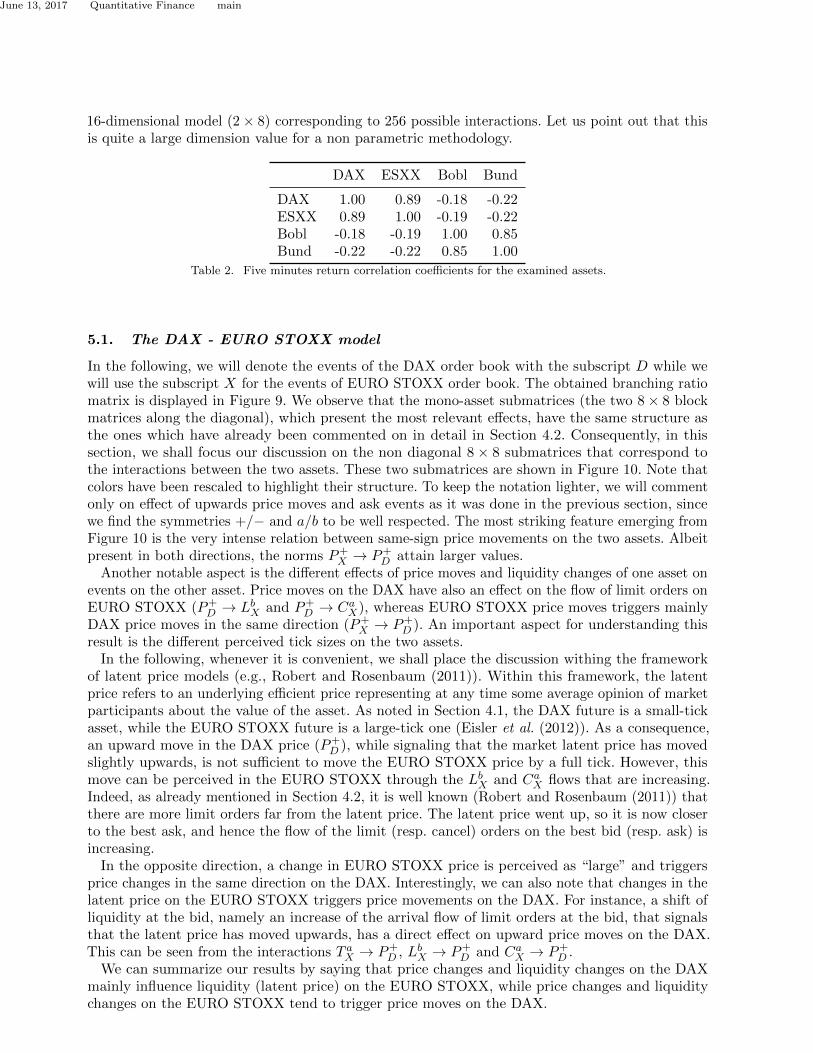
5.1. The DAX - EURO STOXX model

In the following, we will denote the events of the DAX order book with the subscript D while wewill use the subscript X for the events of EURO STOXX order book. The obtained branching ratiomatrix is displayed in Figure 9. We observe that the mono-asset submatrices (the two 8× 8 blockmatrices along the diagonal), which present the most relevant effects, have the same structure asthe ones which have already been commented on in detail in Section 4.2. Consequently, in thissection, we shall focus our discussion on the non diagonal 8 × 8 submatrices that correspond tothe interactions between the two assets. These two submatrices are shown in Figure 10. Note thatcolors have been rescaled to highlight their structure. To keep the notation lighter, we will commentonly on effect of upwards price moves and ask events as it was done in the previous section, sincewe find the symmetries +/− and a/b to be well respected. The most striking feature emerging fromFigure 10 is the very intense relation between same-sign price movements on the two assets. Albeitpresent in both directions, the norms P+

X → P+D attain larger values.

Another notable aspect is the different effects of price moves and liquidity changes of one asset onevents on the other asset. Price moves on the DAX have also an effect on the flow of limit orders onEURO STOXX (P+

D → LbX and P+D → CaX), whereas EURO STOXX price moves triggers mainly

DAX price moves in the same direction (P+X → P+

D ). An important aspect for understanding thisresult is the different perceived tick sizes on the two assets.

In the following, whenever it is convenient, we shall place the discussion withing the frameworkof latent price models (e.g., Robert and Rosenbaum (2011)). Within this framework, the latentprice refers to an underlying efficient price representing at any time some average opinion of marketparticipants about the value of the asset. As noted in Section 4.1, the DAX future is a small-tickasset, while the EURO STOXX future is a large-tick one (Eisler et al. (2012)). As a consequence,an upward move in the DAX price (P+

D ), while signaling that the market latent price has movedslightly upwards, is not sufficient to move the EURO STOXX price by a full tick. However, thismove can be perceived in the EURO STOXX through the LbX and CaX flows that are increasing.Indeed, as already mentioned in Section 4.2, it is well known (Robert and Rosenbaum (2011)) thatthere are more limit orders far from the latent price. The latent price went up, so it is now closerto the best ask, and hence the flow of the limit (resp. cancel) orders on the best bid (resp. ask) isincreasing.

In the opposite direction, a change in EURO STOXX price is perceived as “large” and triggersprice changes in the same direction on the DAX. Interestingly, we can also note that changes in thelatent price on the EURO STOXX triggers price movements on the DAX. For instance, a shift ofliquidity at the bid, namely an increase of the arrival flow of limit orders at the bid, that signalsthat the latent price has moved upwards, has a direct effect on upward price moves on the DAX.This can be seen from the interactions T aX → P+

D , LbX → P+D and CaX → P+

D .We can summarize our results by saying that price changes and liquidity changes on the DAX

mainly influence liquidity (latent price) on the EURO STOXX, while price changes and liquiditychanges on the EURO STOXX tend to trigger price moves on the DAX.

15


Finally, let us note that the above effects are even more pronounced when we estimate theinteraction matrices with a smaller H. In particular the effects of DAX price movements on T, L,Con the EURO STOXX become more relevant compared with those on prices. At the same time,while the effect of EURO STOXX price moves on DAX’s ones is still strong, the effect of liquiditymovements on DAX price movements is comparatively stronger with smaller H. This suggests thatthese effects are mainly localized at short time scales, while the P+ → P+ ones have much slowerdecay in time.

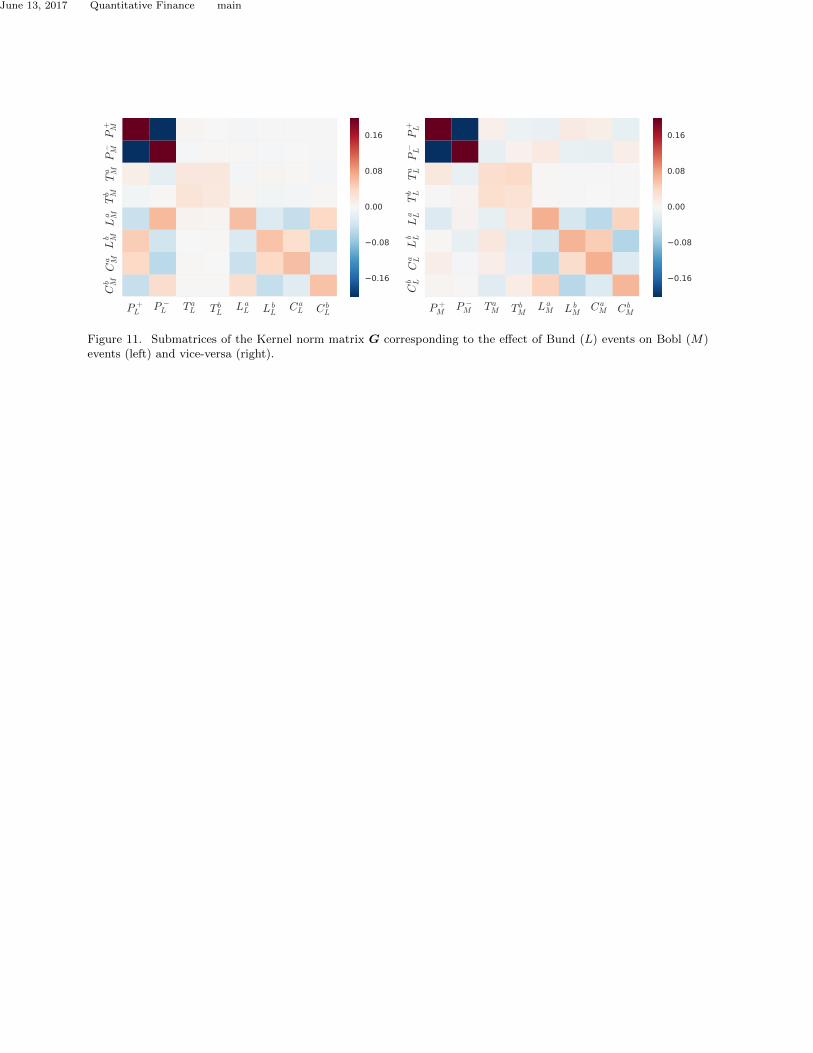
5.2. Bobl - Bund

We perform the same analysis on the asset pair Bobl-Bund futures. Here both assets are largetick assets, however the Bund is much more actively traded than the Bobl in the sense that allthe order flows are of higher intensity. The cross-asset submatrices are depicted in Figure 11. Asin the previous case, we remark that the elements P+

L → P+M and P+

M → P+L reflect the strong

correlation observed between the two assets. Price changes in the Bund have also a noticeable effecton limit/cancel order flows in the Bobl, while price changes in the Bobl have little to no effect onthe Bund except for the mentioned P+

M → P+L interaction. At the same time, T a, La, Ca events on

the Bobl impact prices on the Bund, while the corresponding event on the Bund have little effect.Comparing this with the case of the DAX-EURO STOXX pair, we can liken the effect of the

Bund on the Bobl to that of the DAX over the EURO STOXX and vice-versa. We argue thatthe difference in trading frequency between the Bobl and Bund contracts has a similar effect ofthat of a different tick size that we observed in the previous case. As before, we have an asset, theBund, which is more “reactive” (the limit/cancel order flows are higher than those of the Bobl)than the Bobl, thus a price change of the Bund indicating a change of the latent price impacts thelimit/cancel flows of the Bobl. In the previous case, the higher “reactivity” of the DAX was due toits smaller tick size.

6. Conclusion and prospects

In the context of Hawkes processes, the estimation of the matrix kernel norms is essential, as itgives a clear overview of the dependencies involved in the underlying dynamics. In the contextof high-frequency financial time-series non-parametric estimation of the matrix kernel norms hasalready shown to be very fruitful (Bacry and Muzy (2014), Bacry et al. (2016)), since it provides avery rich summary of the system interactions, and it can thus be a valuable tool in understanding asystem where many different types of events are present. However, its estimation is a computationallydemanding process since these estimations are computed from a non-parametric pre-estimation ofthe kernels themselves, i.e., their entire shape and not only their norm. The resulting complexityprevents the estimations from being performed when the dataset is too heavy or (more important)when the dimension of the Hawkes process (i.e., the number of considered different event types) istoo large.

In this work, we presented the newly developed NPHC algorithm (Achab et al. (2016)) that allowsto directly estimate non-parametrically the kernel norms matrix of a multidimensional Hawkesprocess, that is without going through the kernel shapes pre-estimation step. As of today, it isthe only direct non-parametric estimation procedure available in the academic literature. Thismethod can be seen as a Generalized Method of Moments (GMM) that relies on second-orderand third-order integrated cumulants. This paper shows that this method successfully reveals thevarious dynamics between the different (first level) order flows involved in order books. In a contextof a single-asset 8-dimensional Hawkes process, we have shown (as a “sanity check”) that it is ableto reproduce former results obtained using “indirect” methods. Moreover, the so-obtained gainin complexity allowed us to run a much more detailed analysis (increasing the dimension to 12),separating the different types of events that lead to a mid-price move. This in turn allowed us to

16


have a very precise picture of the high frequency order book dynamics, revealing, for instance, thedifferent interactions that lead to the high-frequency price mean reversion or those between liquiditytakers and liquidity makers as well as the influence of the tick-size of these dynamics. Not the least,through the analysis of the matrix Ψ we also detected the signature of meta-orders. We have alsosuccessfully used the NPHC algorithm in a multi-asset 16-dimensional framework. It allowed usto unveil very precisely the high-frequency joint dynamics of two assets that share exposure tothe same risk factors but that have different characteristics (e.g., different tick sizes or differentdegrees of reactivity). It is noteworthy that our methodology can efficiently highlight these types ofdynamics, especially since cross-asset effects are second order effects compared to mono-asset’s.

We conclude by noting that our study left out some relevant information such as the volumeof the orders and the size of the jumps in the mid-price. This will be the objective of futureworks. Moreover, within the methodology presented in this paper, an analysis of baskets of assets(with more than two assets) as well as multi-agent high-frequency interactions are currently underprogress.

Acknowledgments

This research benefited from the support of the Chair “Changing Markets”, under the aegis of LouisBachelier Finance and Sustainable Growth laboratory, a joint initiative of Ecole Polytechnique,Universite d’Evry Val d’Essonne and Federation Bancaire Francaise and from the chair of the RiskFoundation: Quantitative Management Initiative.

References

Achab, M., Bacry, E., Gaıffas, S., Mastromatteo, I. and Muzy, J.F., Uncovering Causality from MultivariateHawkes Integrated Cumulants. arXiv preprint arXiv:1607.06333, 2016.

Bacry, E., Delattre, S., Hoffmann, M. and Muzy, J.F., Modelling microstructure noise with mutually excitingpoint processes. Quantitative Finance, 2013, 13, 65–77.

Bacry, E., Iuga, A., Lasnier, M. and Lehalle, C.A., Market Impacts and the Life Cycle of Investors Orders.Market Microstructure and Liquidity, 2015a, 01, 1550009.

Bacry, E., Jaisson, T. and Muzy, J.F., Estimation of slowly decreasing Hawkes kernels: application tohigh-frequency order book dynamics. Quantitative Finance, 2016, 16, 1179–1201.

Bacry, E., Mastromatteo, I. and Muzy, J.F., Hawkes Processes in Finance. Market Microstructure andLiquidity, 2015b, 1, 1550005–1550064.

Bacry, E. and Muzy, J.F., Hawkes model for price and trades high-frequency dynamics. Quantitative Finance,2014, 14, 1–20.

Bacry, E. and Muzy, J.F., First- and Second-Order Statistics Characterization of Hawkes Processes andNon-Parametric Estimation. IEEE Transactions on Information Theory, 2016, 62, 2184–2202.

Bormetti, G., Calcagnile, L., Treccani, M., Corsi, F., Marmi, S. and Lillo, F., Modelling systemic pricecojumps with Hawkes factor models. Quantitative Finance, 2015, 15, 1137–1156.

Bowsher, C.G., Modelling security market events in continuous time: Intensity based, multivariate pointprocess models. Journal of Econometrics, 2007, 141, 876 – 912.

Bremaud, P. and Massoulie, L., Stability of nonlinear Hawkes processes. Annals of Probability, 1996, 24,1563–1588.

Da Fonseca, J. and Zaatour, R., Correlation and Lead–Lag Relationships in a Hawkes Microstructure Model.Journal of Futures Markets, 2017, 37, 260–285.

Dayri, K. and Rosenbaum, M., Large tick assets: implicit spread and optimal tick size. Market Microstructureand Liquidity, 2015, 1, 1550003.

Eichler, M., Dahlhaus, r. and Dueck, J., Graphical modeling for multivariate Hawkes processes with nonpara-metric link functions. Journal of Time Series Analysis, 2017, 38, 225–242.

Eisler, Z., J.-P., B. and Kockelkoren, J., The price impact of order book events: market orders, limit ordersand cancellations. Quantitative Finance, 2012, 12, 1395–1419.

17


Filimonov, V. and Sornette, D., Quantifying reflexivity in financial markets: Toward a prediction of flashcrashes. Physical Review E, 2012, 85, 056108.

Hall, A., Generalized Method of Moments, 2005, Oxford university press.Hansen, L., Large sample properties of generalized method of moments estimators. Econometrica: Journal of

the Econometric Society, 1982, pp. 1029–1054.Hardiman, S. and Bouchaud, J.P., Branching-ratio approximation for the self-exciting Hawkes process. Phys.

Rev. E, 2014, 90, 062807.Hardiman, Stephen J., Bercot, Nicolas and Bouchaud, Jean-Philippe, Critical reflexivity in financial markets:

a Hawkes process analysis. Eur. Phys. J. B, 2013, 86, 442.Hawkes, A. and Oakes, D., A Cluster Process Representation of a Self-Exciting Process. Journal of Applied

Probability, 1974, 11, 493–503.Hayashi, T., Yoshida, N. et al., On covariance estimation of non-synchronously observed diffusion processes.

Bernoulli, 2005, 11, 359–379.Jedidi, A. and Abergel, F., On the stability and price scaling limit of a Hawkes process-based order book

model. Available at SSRN: https://ssrn.com/abstract=2263162, 2013.Jovanovic, S., Hertz, J. and Rotter, S., Cumulants of Hawkes point processes. Physical Review E, 2015, 91,

042802.Large, J., Measuring the resiliency of an electronic limit order book. Journal of Financial Markets, 2007, 10,

1–25.Lewis, E. and Mohler, G., A nonparametric EM algorithm for multiscale Hawkes processes. preprint, 2011.Ogata, Y., On Lewis’ simulation method for point processes. Information Theory, IEEE Transactions on,

1981, 27, 23–31.Rambaldi, M., Bacry, E. and Lillo, F., The role of volume in order book dynamics: a multivariate Hawkes

process analysis. Quantitative Finance, 2016, pp. 1–22.Reynaud-Bouret, P., Rivoirard, V., Grammont, F. and Tuleau-Malot, C., Goodness-of-fit tests and nonpara-

metric adaptive estimation for spike train analysis. The Journal of Mathematical Neuroscience (JMN),2014, 4, 1–41.

Robert, C. and Rosenbaum, M., A New Approach for the Dynamics of Ultra-High-Frequency Data: TheModel with Uncertainty Zones. Journal of Financial Econometrics, 2011, 9, 344.

Toke, I.M., Market making in an order book model and its impact on the spread. In Econophysics ofOrder-driven Markets, pp. 49–64, 2011, Springer.

Xu, H., Farajtabar, M. and Zha, H., Learning Granger Causality for Hawkes Processes. In Proceedings of theProceedings of The 33rd International Conference on Machine Learning, pp. 1717–1726, 2016.

Yang, S.H. and Zha, H., Mixture of mutually exciting processes for viral diffusion. In Proceedings of theProceedings of the International Conference on Machine Learning, 2013.

Zhou, K., Zha, H. and Song, L., Learning Social Infectivity in Sparse Low-rank Networks Using Multi-dimensional Hawkes Processes. AISTATS, 2013a.

Zhou, K., Zha, H. and Song, L., Learning triggering kernels for multi-dimensional Hawkes processes. InProceedings of the Proceedings of the International Conference on Machine Learning, pp. 1301–1309, 2013b.

Appendix A: Origin of the scaling coefficient κ

Following the theory of GMM, we denote m(X, θ) a function of the data, where X is distributedwith respect to a distribution Pθ0 , which satisfies the moment conditions g(θ) = E[m(X, θ)] = 0 ifand only if θ = θ0, the parameter θ0 being the ground truth. For x1, . . . , xN observed copies of X,

we denote gi(θ) = m(xi, θ), the usual choice of weighting matrix is WN (θ) = 1N

∑Ni=1 gi(θ)gi(θ)

>,and the objective to minimize is then

(1

N

N∑i=1

gi(θ)

)(WN (θ1)

)−1(

1

N

N∑i=1

gi(θ)

), (A1)

18


where θ1 is a constant vector. Instead of multiplying by the inverse weighting matrix, we havedecided to divide by the sum of its eigenvalues, which is easily computable:

Tr(WN (θ)) =1

N

N∑i=1

Tr(gi(θ)gi(θ)>)

=1

N

N∑i=1

Tr(gi(θ)>gi(θ))

=1

N

N∑i=1

||gi(θ)||22

In our case, g(R) =[vec[Kc −Kc(R)],vec[C −C(R)]

]>∈ R2d2 . Assuming the associated

weighting matrix is block-wise, one block for Kc −Kc(R) and the other for C −C(R), the sum of

the eigenvalues of the first block becomes ‖Kc −Kc(R)‖22, and ‖C −C(R)‖22 for the second. Wecompute the previous terms with R1 = 0. All together, the objective function to minimize is

1

‖Kc‖22‖Kc(R)− Kc‖22 +

1

‖C‖22‖C(R)− C‖22, (A2)

which equals the loss function given in 16, up to a constant.

19


P+ D

P− D Ta D

Tb D

La D

Lb D

Ca D

Cb D

P+ X

P− X Ta X

Tb X

La X

Lb X

Ca X

Cb X

C bX

C aX

L bX

L aX

T bX

T aX

P −X

P +X

C bD

C aD

L bD

L aD

T bD

T aD

P −D

P +D

2

1

0

1

2

Figure 9. Hawkes kernel norm matrix obtained when the DAX and EURO STOXX futures are considered simulta-neously in a 16D model. DAX events are denoted with the D subscript, EURO STOXX ones with the X subscript.

P +D

P −D T aD T bD L a

D L bD

C aD C b

D

Cb X

Ca X

Lb X

La X

Tb X

Ta X

P− X

P+ X

0.2

0.1

0.0

0.1

0.2

P +X

P −X T aX T bX L a

X L bX

C aX C b

X

Cb D

Ca D

Lb D

La D

Tb D

Ta D

P− D

P+ D

0.2

0.1

0.0

0.1

0.2

Figure 10. Submatrices of the Kernel norm matrix G corresponding to the effect of DAX events on EUROSTOXXSTOXX events (left) and vice versa (right). These two submatrices correspond to the ones lying on the antidiagonalon the Figure 9

20


P +L

P −L T aL T bL L a

L L bL

C aL C b

L

Cb MCa MLb MLa MTb MTa MP− MP

+ M

0.16

0.08

0.00

0.08

0.16

P +M

P −M T aM T bM L a

M L bM

C aM C b

M

Cb LCa LLb LLa LTb LTa LP− LP

+ L

0.16

0.08

0.00

0.08

0.16

Figure 11. Submatrices of the Kernel norm matrix G corresponding to the effect of Bund (L) events on Bobl (M)events (left) and vice-versa (right).

21

estimation of the branching ratio matrix - arxiv.org · june 13, 2017 quantitative finance main to...

Documents