estimation of reservoir properties from...
TRANSCRIPT


ii
Estimation of Reservoir Properties from Seismic Attributes and Well Log Data using Artificial Intelligence
By
MOHAMED SITOUAH
A Thesis Presented to the DEANSHIP OF GRADUATE STUDIES
KING FAHD UNIVERSITY OF PETROLEUM & MINERALS DHAHRAN, SAUDI ARABIA
In Partial Fulfillment of the Requirements for the Degree of
MASTER OF SCIENCE
In
GEOPHYSICS
June 2009

iii

iv
Dedicated
To my Loving Parents and my loving wife

v
ACKNOWLEDGEMENT
All gratitude belongs to Almighty Allah SWT the lord of the universe, who teaches man
what he knows not. I thank Allah for having spared my life over the years and for
bestowing on me His uncompromising blessings.
First, I like to acknowledge the opportunity given to me by King Fahd University of
Petroleum and Minerals and especially Department of Earth Sciences to pursue my
master degree in a harmonious environment with state-of the-art facilities.
My thanks are due to Dr.Al-Shaibani the Chairman of ESD, for his support and help.
My immense appreciation and gratitude goes to my thesis advisor Prof. Gabor. Korvin
and co-advisor Dr. Abdulatif Al-Shuhail, for their guidance, encouragement and support
during the research. Most important of all were their enthusiastic approach towards
research and their readiness and eagerness to help me at any times. Additionally their
innovative thinking and valuable suggestions greatly inspired me. I thank them, as they
are indeed not only advisors but fathers to reckon with.
My sincere gratitude is due to my thesis committee members: Dr.Abdulatif. Osman, Dr.
Abdulazeez. AbdulaReheem and Dr. Azedine. Zerguine. Their constructive and positive
criticism and suggestions were extremely helpful and an immense privilege.
I also want to acknowledge the support and suggestions of my friends and colleagues:
Maamer Al-Djabri, Ali Al-Rayeh and Fayçal Belaid.

vi
TABLE OF CENTENTS DEDICATE……………………………………………………………………………………...iii ACKNOWLEDGMENT……………………………………..…………………………………iV TABLE OF CONTENT………………………………………………….………………………V LIST OF TABLES………………………………………………………………….…………...iX LIST OF FIGURES…………………………………………………………………………..….X THESIS ABSTRACT ......................................................................................................... xv
الرسالة ملخص ........................................................................................................................ xvii
CHAPTER ONE
Introduction ..........................................................................................................................1
1.1 Overview .......................................................................................................................1
1.2 Problem Statement ........................................................................................................3
1.3 Thesis Objectives ...........................................................................................................4
1.4 Thesis Organization ......................................................................................................4
1.5 Literature review ...........................................................................................................5
CHAPTER TWO
Geological Setting of Study Area ..........................................................................................7
2.1 Overview .......................................................................................................................7
2.2 Regional Geological description of the basin ..................................................................9
2.2.1 The Southern accident atlas: .......................................................................................... 9
2.2.2 The Paleozoic of the Sahara: ......................................................................................... 9
2.2.3 The Lower and the Middle Jurassic (Lias-Dogger) ......................................................... 9
2.2.4 The Upper Jurassic ................................................................................................... 10
2.2.5 The Lower Cretaceous ............................................................................................... 11
2.2.5.1 Barremian……….. ................................................................................................... 11
2.2.5.2 Aptian………………. ............................................................................................... 11
2.2.5.3 Albian…………….. ................................................................................................. 11
2.2.5.4 Cenomanian……… .................................................................................................. 12
2.2.5.5 Turonian………….. ................................................................................................... 12
2.2.5.9 Eocene………………… ............................................................................................ 13
2.2.5.10 The Quaternary ...................................................................................................... 13
vii
2.3 Local geological framework ......................................................................................... 16
2.4 The Geological Structure of the Study Area ................................................................ 18
2.5 Geological History of the Study Area ............................................................................. 19
2.6 The characteristics of the Source Rock ........................................................................ 20
2.7 Sedimentary facies Analysis ........................................................................................ 23
2.7.1 Fluvial-channel lag deposit ...................................................................................... 24
2.7.2 Point bar deposit ...................................................................................................... 24
2.7.3 Channel bar sedimentary .......................................................................................... 24
2.7.4 Over bank deposit .................................................................................................... 25
2.7.5 Crevasse splay deposit ............................................................................................. 25
2.8 Reservoir Properties .................................................................................................... 25
2.9 Cap rock characteristics .............................................................................................. 30
2.10 Migration System ........................................................................................................ 31
CHAPTER THREE
3.1 Introduction .................................................................................................................. 32
3.2 Definitions ................................................................................................................... 32
3.4 Classification of Seismic Attributes ............................................................................. 34
3.4.1Geometrical attributes (reflection configuration)………................................................ 34
3.4.2Physical attributes (reflection characteristics)…. .......................................................... 35
3.4.3 Pre-stack Attributes ............................................................................................... 35
3.4.5 Instantaneous Attributes ......................................................................................... 36
3.4.7 Reflection Attributes .................................................................................................. 36
3.4.8 Transmissive Attributes ............................................................................................. 36
3.5 Hilbert Transform ....................................................................................................... 38
3.5.1 Definition of the Hilbert Transform ............................................................................... 38
Figure 3.2 Hilbert Filter ...................................................................................................... 39
3.5.2 Properties of Hilbert Transform .............................................................................. 39
3.5.3 Discrete Hilbert Transform ...................................................................................... 40
Figure 3.3 Impulse Response of Hilbert Transform ............................................................ 43
3.6 Computation of Seismic Attributes .............................................................................. 44
3.6.1 Formulation of Seismic Attributes ............................................................................ 45
CHAPTER FOUR
Artificial Neural Networks .................................................................................................. 52
viii
4.1 Definition .................................................................................................................... 52
4.2 Historical background of Neural Networks.......................................................... 52
4.2 Comparison between Artificial neurons and Human ................................................... 56
4.3.1 a simple neuron ........................................................................................................ 57
4.3.2 Firing rules ............................................................................................................. 58
4.3.3 How the firing rule works ........................................................................................ 59
4.4 Neural network structure ........................................................................................... 60
4.4.1 Feed-forward networks ............................................................................................ 61
4.4.2 Adaptive networks .................................................................................................... 62
4.5 The Mathematical Model (figure 4.5) .......................................................................... 64
4.6 Multilayer Perceptron Neural Network (MLP) ........................................................... 70
4.6.1 The Network Performance ....................................................................................... 75
4.6.2 Testing (Generalizing) ............................................................................................... 76
4.6.3 Advantages and disadvantages of MLP ..................................................................... 77
4.7 General Regression Neural Networks .......................................................................... 79
4.7.1 Advantages and disadvantages of GRNN .................................................................. 83
CHAPTER FIVE
5.1 Overview ..................................................................................................................... 84
5.2 DATA ANALYSIS ...................................................................................................... 85
5.3 Experimental Results Using Mutilayer Perception and General Regression Neural Networks ............................................................................................................................ 87
5.3.1 Porosity Estimation Results From Well Logs ............................................................. 87
5.3.2 Permeability Estimation Results From Well Logs ...................................................... 92
5.3.3 Porosity Estimation Results From Seismic Attributes ................................................. 97
5.3.4 GRNN MODEL FOR POROSITY ......................................................................... 107
5.3.5 GRNN MODEL FOR PERMEABILITY ................................................................ 109
5.4 Predicting Porosity and Permeability using Well logs and Seismic Attributes ............... 111
5.4.1 GRNN MODEL FOR POROSITY ......................................................................... 112
5.4.2 GRNN MODEL FOR PERMEABILITY ................................................................ 115
5.5 Prediction of Lithofacies Using ANNs........................................................................ 117
Figure 4.14b Facies Predictions using ANNs ..................................................................... 118
5.6 Predicting the Spatial Distribution of Porosity, Permeability and Lithofaces ............. 119

ix
5.6.1 Porosity Models .................................................................................................... 120
5.6.2 Permeability Models .............................................................................................. 122
5.6.3 Lithofacies models ................................................................................................ 124
CHAPTER SIX
6.1 Summary .................................................................................................................. 128
6.2 Conclusions ............................................................................................................... 129
References ........................................................................................................................ 131

x
LIST OF TABLES
Table 2.1: The main reservoirs in the study area and their Properties…………………...26
Table4.1: The truth table…………………………………………...………………….…59
Table 5.1: Statistics of the combined wells 1 and 2 (Training set)…...……………….…86
Table 5.2: Statistics of the combined wells 1 and 2 (Testing set)………..........................86
Table 5.3 Results Summary for MLP and GRNN models……...…………………….….96
Table 5.4 Statistical Properties of the Seismic Attributes (Training set)……………..….97
Table 5.5 Statistical Properties of the Seismic Attributes (Testing set)…………………97
Table 5.6 Statistical Analysis for Seismic and Logs (Training data)…………………..111
Table 5.7 Statistical Analysis for Seismic and Logs (Testing data)…...……………….112

xi
LIST OF FIGURES
Figure 2.1: Satellite Image of the Study area……………………………….………….….7
Figure2.2: Geographical Map of the Study Area………………………………….……...8
Figure 2.3: Origin of Sands of Lower Cretaceous………………………………………10
Figure 2.4: Regional geological Map showing the geological time of each
zone……………………………………………………………………..………………..14
Figure 2.5: Stratigraphic Colum of the Northeast of Sahara showing the main lithology in
each stage…………………………………………..……………………………….……15
Figure 2.6: Maturation in the Lower Silurian Radioactive Clays…........................……22
Figure 2.6 b: TOC Distribution in the Lower Silurian Radioactive Clays………………23
Figure.2.7a: Porosity Distribution within lower Ordovician…………………….………27
Figure 2.7 b. Porosity Distribution within upper Ordovician…………….…………...…28
Figure 2.7c: Porosity distribution within Triassic………………………..……...….……29
Figure 2.8: Distribution of Clay & Evaporate deposits from Triassic & Liassic.........................................................................................................................…...31
Figure 3.1: Seismic attributes Classification………………………………........………37
Figure .3.2: Hilbert Filter…………………………………………………….………....39 Figure 3.3: Impulse response of Hilbert Transform………………………........……….43
Figure.4.1: Comparison between Artificial neurons and
Human neurons…………………………………………………………….…………… 57

xii
Figure 4.2: a simple neuron ………………………………………………………...…58
Figure 4.3: Feed Forward Networks Structure………………..………………………....61
Figure 4.4: Supervised Learning Scheme ........................................................................64
Figure 4.5: Mathematical model of ANNs ………………………………..……………65
Figure 4.6: Pure linear function…………………………………………………..…..…67
Figure 4.7: Threshold function……………………………...……………...……….…..68
Figure 4.8: Sigmoid Function …………………………………………………………...69
Figure 4.9: Tangent Hyperbolic Function for a =1………………………………….…...70
Figure 4.10: Multilayer Perceptron with two hidden layers……………………………..71
Figure.4.11 Typical GRNN architecture………………………………………………...79
Figure.4.12: Radial Basis Transfer Function for one input……………………………...81
Figure.4.13: Radial Basis Transfer Function for multi inputs………….....................….82
Figure 5 .1a: Training core porosity vs predicted porosity
using MLP……………………………………………………………………………....88
Figure 5.1b: Testing core porosity vs predicted porosity
using MLP………………………………………………………………………………89
Figure 5.2a: Training core porosity vs predicted porosity
using GRNN………………………………………………………………………….…90
Figure 5.2b: Testing core porosity vs predicted porosity
using GRNN…………………………………………………………………………..…91
Figure 5.3a:Training core permeability vs predicted permeability
using MLP……………………………………………………………………………….93
Figure 5.3b: Testing core permeability vs predicted permeability
using MLP…………………………………………………………………………….....94
xiii
Figure 5.4a: Training core permeability vs predicted permeability
using GRNN……………………………………………………….………………...….95
Figure 5.4b: Testing core permeability vs predicted permeability
using GRNN………………………………………………………………………..……96
Figure 5.5: Base map of the study area………………………………..…………………98
Figure 5.6: 3D Seismic Volume of the study site……………………..…………………99
Figure 5.7: Top of T1 on base map……………………………………………………..100
Figure 5.8a: 3D Volume of Instantaneous Frequency…………………….……………101
Figure 5.8b: 3D Volume of RMS amplitude…………………………………………...102
Figure 5.9a: Time slice of the Instantaneous Frequency at 2ms…………...…………...103
Figure 5.9b: Time slice of the Instantaneous Frequency at 8ms………………………..103
Figure 5.9c: Time slice of the Instantaneous Frequency at 12ms……..........…………..104
Figure 5.9d: Time slice of the Instantaneous Frequency at 20ms…...........…………….104
Figure5.10a: Time slice of the Instantaneous Phase at 2ms…………….……………...105
Figure 5.10b: Time slice of the Instantaneous Phase at 6ms……………….…..............105
Figure 5.10c: Time slice of the Instantaneous Phase at 10ms……………..…..............106
Figure 5.10d: Time slice of the Instantaneous Phase at 12ms………………..………...106
Figure 5.11a :Training core porosity vs predicted porosity
using GRNN…………………………………………...……………………………….107
Figure 5.11b :Testing core porosity vs predicted porosity
using GRNN……………………………………………………………………………108
Figure 5.12c :Training core permeability vs predicted permeability
using GRNN……………………………………………………………….…………...109
Figure 5.12d: Training core permeability vs predicted permeability
using GRNN………………………………………………………..………..………...110

xiv
Figure 5.13a Training core porosity vs predicted porosity
using GRNN (Logs + Attributes)………………………………..……………………...113
Figure 5.13b Testing core porosity vs predicted porosity
using GRNN (Logs + Attributes)……………………………………….………………114
Figure 5.13c Training core permeability vs predicted permeability
using GRNN (Logs + Attributes)……………………………………………...………..115
Figure 5.13d: Testing core permeability vs predicted permeability
using GRNN (Logs + Attributes)…………………………............……………..……..116
Figure 5.14a: Facies Description of Well-1 and Well-2………………………………..117
Figure 5.14b: Facies Predictions (in column # 4) using ANNs…………….………….118
Figure 5.15: Seismic Interpretation of T1, SI and Dev reservoirs
in the study area……………………………………………………….………………119
Figure 5.16a: Histogram of the porosity distribution.....................................................120
Figure 5.16b: Porosity distributions in the 3D model for SI reservoir...........................121
Figure.5.16c: Porosity (10% - 30 %) distribution in the 3D model for SI reservoir………………………………………………………………………………...121
Figure 5.17 Histogram of permeability distribution…………………………………...122
Figure 5.17 a. Permeability Distribution in 3D model for SI reservoir…………...…....123
Figure 5.17b: Permeability (10-300 mD) distribution for SI reservoir……………..….123
Figure 5.18: Histogram of facies distribution …………………………...………….…124
Figure 5.18a: Facies model of SI and Dev reservoirs………………………………….125
Figure 5.18b: Channel lag distribution for SI Reservoir …………..…………………..126
Figure 5.18.c. Point bar distribution for SI Reservoir ………………………………....126
Figure 5.18d: Over bank distribution for SI Reservoir …………..……………………127

xv
THESIS ABSTRACT
NAME: Mohamed Sitouah TITLE OF STUDY: Estimation of Reservoir Properties from
Seismic Attributes and Well Log Data Using Artificial Intelligence
MAJOR FIELD: Geophysics DATE OF DEGREE: June, 2009 Permeability, Porosity and Lithofacies are key factors in reservoir
characterizations. Permeability, or flow capacity, is the ability of porous rocks to transmit
fluids, porosity, represent the capacity of the rock to store the fluids, while lithofacies,
describe the physical properties of rocks including texture, mineralogy and grain size.
Many empirical approaches, such as linear/non-linear regression or graphical techniques.
Were developed for predicting porosity, permeability and lithofacies. Recently,
researches used another tool named Artificial Neural Networks (ANNs) to achieve better
predictions. To demonstrate the usefulness of Artificial Intelligence technique in
geoscience area, we describe and compare two types of Neural Networks named
Multilayer Perception Neural Network (MLP) with back propagation algorithm and
General Regression Neural Network (GRNN), in prediction reservoir properties from
seismic attributes and well log data.

xvi
This study explores the capability of both paradigms, as automatique systems for
predicting sandstone reservoir properties, in vertical and spatial directions. As it was
expected, these computational intelligence approaches overcome the weakness of the
standard regression techniques.
Generally, the results show that the performances of General Regression neural networks
outperform that of Multilayer Perceptron neural networks. In addition, General
Regression Neural networks are more robust, easier and quicker to train. Therefore, we
believe that the use of these better techniques will be valuable for Geoscientists.

xvii
ملخص الرسالة
محمد ستواح :الكامل اإلسم
تقدير خصائص المكامن من المعطيات السيزمية و بيانات اآلبار :عنوان الرسالة باستخدام الذآاء الصناعي
جيزفيزياء :التخصص
٢٠٠٩جوان :تاريخ الشهادة
هو النفاذية ، أو تدفق القدرة ،. هي عوامل رئيسية في تحديد خصائص المكمن المسامية، النفاذية والسحن الصخري
وصف السحن الصخري فهو بينما قدرة الصغور لنقل السوائل ، المسامية ، تمثل قدرة الصخر لتخزين السوائل ،
توجد الكثير من الطرق التجربية للتنبأ بالنفاذية، .والمعادن الحبوب حجم الملمس منالخصائص الفيزيائية للصخور
.المسامية و السحن الصخري ، مثل االنحدار الخطي و االنحدار الالخطي و آذا الطرق البيانية
هذه الطرق أثبتت محدويتها في هذا المجال عندما يتعلق األمر بتنبأ خصائص المكامن الغير متجانسة حيث أن
.رات في خصائص المكمن تجعل من الصعوبة بمكان التنبأ بخصائصهالتغي
لتحقيق مستوى أفضل من) ANNs(أداة أخرى للبحوث اسمها الشبكات العصبية االصطناعية مؤخرا ، استخدم
إلثبات جدوى تقنية الذآاء االصطناعي في مجال علوم األرض ، قمنا بإجراء مقارنة بين نوعين من . التوقعات
و ذلك باستعمال المعطيات السيزمية و ). MLP( و الثاني (GRNN )ت العصبية النوع األول يسمى الشبكا
.تسجبل بيانات المكامن
ن البترولية آالمسامية، النفاذية المكامفي هذا البحث تم تناول قدرة آلتا الشبكتين العصبيتين على تنبأ بعض خصائص
على تنبأ ) GRNN( دراسة أثبتت نجاعت و قدرة الشبكة العصبية المسماة عموما نتائج هذه ال .و السحن الصخري
باالضافة ). MLP( خصائص المكمن و بدقة عالية تفوق تلك التي تم تقديرها باستعمال الشبكة الثانية المسماة

xviii
التقنيات المتطورة سيساعد لهذا نعتقد أن استعمال هذه . أآثر سرعة و أآثر قوة) GRNN( الى أن الشبكة العصبية
و يعطي نظرة أوضح للجيولوجيين و الجيوفيزيائين في تقدير حرآة السوائل داخل أآثر في تطوير المكامن البترولية
.المكمن

1
CHAPTER ONE
Introduction
1.1 Overview
Reservoir characteristics can be divided into three groups: geological characteristics
(structure and seal, lithology, diagenesis), engineering data (well spacing, well-bore
integrity, etc.) and rock-fluid properties (porosity, permeability, resistivity, etc.), (see
James and Lawrence , 2002). Porosity, permeability and lithofacies are key factors for
reservoir modeling. Permeability is the ability of the porous rock to transmit fluid, it
depends on the statistics of the pore throat diameters rather than of the pore size, and is
related to effective porosity rather than the total porosity.
Lithofacies identification is a primary task in reservoir characterization; it is achieved by
studying a combination of petrophysical and petrographical properties of the rock. In
general, when core samples are taken from rocks, they are described and classified into
categories called “Facies” or “Lithofacies”. Such lithofacies represent a well defined rock
type (e.g. sandstone, limestone, dolomite, etc.). To build a 3D geological model for a
reservoir, accurate knowledge of permeability, porosity and lithofacies is required. The
best method to get accurate values for these three factors is to measure them directly in
the laboratory; however, this method has some disadvantages: its high cost, being time
consuming, and incomplete representation of the total depth range. For these reasons
geologists often core only a few out of all

2
wells and even then only a small portion of the well. Geologists generally use a statistical
approach, such as linear or non-linear multiple regressions (Wendt et al.,1981; Jensen et
al. 1985) to correlate different reservoir properties (such as: porosity and permeability).
In these approaches, a linear or non-linear relationship is assumed between permeability
and other reservoir properties. However, these techniques have proved inadequate for
certain geological problems like heterogeneous reservoirs (Moline and Bahr, 1995).
Recently, geoscientists have utilized methods of Artificial Intelligence (AI), especially
Neural Networks (NNs), to predict reservoir properties. Neural Networks have been
widely used in many fields of science and engineering (e.g. in economy to predict
chaotic stock market behavior, or to optimize financial portfolios). In Petroleum Industry,
Neural Networks have been used to predict fracture intensity (Boevner et al., 2003;
Ouenes et al., 1998), for field development (Dorusamy, 1997), for litho-facies analysis
(Tanmbasu et al., 2004), to predict irreducible water saturation (Goda et al., 2007), to
predict drilling hydraulics in real time (Fruhwirth et al., 2007), and for other purposes,
such as to optimize hydraulic fracture designs, characterize oil and gas reservoirs,
optimize drilling operation, interpret well logs, generate virtual magnetic resonance logs,
and to select candidate wells for reservoir stimulation.
Artificial Neural Networks are powerful tools for modeling nonlinear, complex systems.
They are distributive, parallel systems, very useful to deal with pattern recognition
problems. They are able to predict complex relationships between several variables (e.g.
between well log data and seismic attributes, permeability, porosity and rock types).
However, Neural Networks are black-box models that use activation functions of a
predefined form (but with parameters adjusted through learning) and a predefined
3
architecture (number of hidden layers, number of neurons in each layer), without duly
considering the specific properties of the phenomena being modeled.
Computer scientists in the field of Machine Learning and Data Mining have found
several alternative methods to get over the limitations of Neural Networks. One of the
popular methods is Adaptive Neural Fuzzy Inference System (ANFIS), which is a new
framework, dealing with prediction and classification problems.
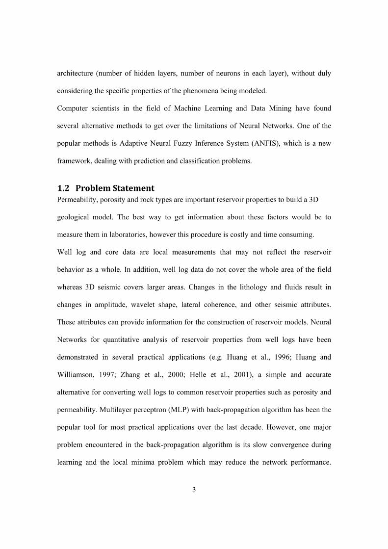
1.2 Problem Statement Permeability, porosity and rock types are important reservoir properties to build a 3D
geological model. The best way to get information about these factors would be to
measure them in laboratories, however this procedure is costly and time consuming.
Well log and core data are local measurements that may not reflect the reservoir
behavior as a whole. In addition, well log data do not cover the whole area of the field
whereas 3D seismic covers larger areas. Changes in the lithology and fluids result in
changes in amplitude, wavelet shape, lateral coherence, and other seismic attributes.
These attributes can provide information for the construction of reservoir models. Neural
Networks for quantitative analysis of reservoir properties from well logs have been
demonstrated in several practical applications (e.g. Huang et al., 1996; Huang and
Williamson, 1997; Zhang et al., 2000; Helle et al., 2001), a simple and accurate
alternative for converting well logs to common reservoir properties such as porosity and
permeability. Multilayer perceptron (MLP) with back-propagation algorithm has been the
popular tool for most practical applications over the last decade. However, one major
problem encountered in the back-propagation algorithm is its slow convergence during
learning and the local minima problem which may reduce the network performance.

4
Thus, to overcome the drawbacks of multi-layer perceptron neural networks, we are
interested in designing and investigating some more adequate intelligent system
techniques which have been proposed as an improvement to neural networks, and can be
utilized in estimation of porosity and permeability.
1.3 Thesis Objectives
The main objective of this research work is to explore new techniques developed by
computer scientist particularly neural networks to predict reservoir properties such us
porosity, permeability and rock types in vertical and spatial directions from well log data
and seismic attributes. This study aims to develop the best approach for the estimation of
these properties. More specifically this work aims to achieve the following
1. Investigate and develop a multi layer perceptron (MLP) to estimate porosity and
permeability from well log data.
2. Investigate the suitability of estimating porosity and permeability from well logs
using general regression neural network (GRNN).
3. Compare the above two techniques and choose the better one.
4. Estimate porosity and permeability from seismic attributes using the selected
algorithm.
5. Build a 3D model for the properties estimated by the selected neural network.
1.4 Thesis Organization
In the introductory Chapter one, I highlight the motivation behind this work. Chapter two
describes the geological setting of the study area and the main reservoirs. Chapter three

5
deals with seismic attributes calculation and analysis. The main technique, neural
networks are discussed in detail in Chapter four. In Chapter five I discuss the results
provided by MLP and GRNN and investigate the performance of both techniques in
estimating reservoir properties. Finally, conclusions and recommendations will be given
in Chapter six.
1.5 Literature review
Porosity, permeability and lithofacies are very important factors in geological modeling.
Many empirical approaches are available to estimate these reservoir properties such as
linear/non-linear multiple regression. Recently, geoscientists benefited from the fast
development in computer science, and used other, non standard approaches to solve
complicated geological problems, related to reservoir heterogeneity (e.g.: permeability
and lithofacies distributions). The following discussion focuses on the use of Artificial
Neural Networks (NNs) in prediction reservoir properties.
Mohaghegh et al. (1991, 1997) designed a Neural Network model for permeability
determination from well log data. Smith et al. (1991) used a distributed Neural Network
to identify the presence of lithographic facies types in an oil well, using only the readings
obtained by a log probe. Hsien-Cheng et al. (1991) presented a hybrid system consisting
of three adaptive resonance-theory NNs and a rule-based expert system to identify
lithofacies from well log data. Rogers et al. (1992) also determined lithology from well
logs using NNs. Huang (1996) used NNs to predict permeability in a venture gas field
offshore eastern Canada. Olson (1998) used NNs to predict porosity and permeability in
a low permeability gas reservoir based on well log data. Garrouch et al. (1998) used a

6
back-propagation NN to estimate tight gas sand and permeability from porosity, mean
pore size and mineralogical data. Tamhane (2000) presented an overview of soft
computing technologies for reservoir characterization, including Neural Networks, fuzzy
logic and evolutionary algorithms. Soto et al. (2000, 2001) developed an integrated
concept of multi-variant statistical analysis, Neural Networks and Fuzzy Logic to predict
reservoir properties on uncored wells. Jong et al. (2004) combined fuzzy logic and neural
networks to predict reservoir porosity and permeability from well log data.
Tanwi et al. (2004) integrated core data and log data for facies analysis using NNs. Ferraz
and Garcia (2005) made a comparative study of four different techniques: traditional
discriminant analysis, neural networks, fuzzy logic and neuro-fuzzy system, to determine
the rock's lithofacies. El-shafei and Hamada (2007) used NNs to identify the
Hydrocarbon Potential of shaly sand reservoirs.

7
CHAPTER TWO
Geological Setting of Study Area
2.1 Overview The study area is situated in the North East of the Algerian Sahara (Figures 2.1 and 2.2).
The exploration area is 4353.46KM2 and its surface altitude is about 230M.
Figure 2.1 Satellite Image of the Study area ( Google Earth)

8
Figure2.2 Geographical Map of the Study Area (Bellaoueur.A, 2008)

9
2.2 Regional Geological description of the basin There have been a great number of published articles and reports on the geology of the
sedimentary basin of the Sahara (Busson, 1970; Conrad, 1969 and Dubief, 1959).
The study is located in the sedimentary basin of Oued Mya, North-Eastern Sahara, whose
large geologic features are given below.
2.2.1 The Southern accident atlas: Its separates the Maghrebian mobile zone from the remainder of Western Africa. The
rigid shield is made of sedimentary and eruptive, folded and metamorphosed rocks.
2.2.2 The Paleozoic of the Sahara: It corresponds to the deposits of periglacial desert climate. Around the outcrops of the
base, sandy and schist layers of Tassilis are staged. The Hercynian movements caused the
erosion of the shield, then settled a great continental period during the Triasic
(Busson, 1970). TheTriassic is divided into large distinct lithological units which can be:
salty, argillaceous, argilo-sandy or carbonate. The thickness of these various formations
varies mainly where salty benches are intercalated. The thickness of Triassic shaly-sand
increases towards the North-West (150-180 m) and decreases in the zones of Hassi
Messaoud and R. El Baguel. Triassic has a thickness of 700 m in the N-E of Ghadamès
and which reaches 1300 m in H. Messaoud.
2.2.3 The Lower and the Middle Jurassic (Lias-Dogger) It consists of mainly evaporate layers primarily made up of salt, anhydrite and clays
which are superimposed in marine layers and which are presented in the form of
limestones and clays with anhydrite benches. The Middle Jurassic is characterized by a

10
transgression covering all the basin of the Great Eastern Erg and the deposits are thick
there.
2.2.4 The Upper Jurassic It is characterized by a relative permanence of the marine mode with sediments of
confined surroundings. In the Western part of the basin, the marine mode shows a certain
regression .The passage of the upper Jurassic to the lower Cretaceous is characterized by
terrigenous contributions having for origin the feeder reliefs located at the South of the
Saharan basin (Hoggar) (Figure.2.3) (Busson, 1970).
Figure 2.3 Origin of Sands of Lower Cretaceous (Ouaja, 2003)

11
2.2.5 The Lower Cretaceous
The study of core data (Busson, 1970) made possible to specify the succession of
paleogeography in the lower Cretaceous. It consists of fluvio-deltaic layers which are in
lithological and sedimentary contrast with the marine deposition of the upper Jurassic . It
include the following:
2.2.5.1 Barremian It is characterized by a spreading of the detrital formations of the Lower Cretaceous into
the Low-Sahara. These formations arise in the form of fine to coarse sandstones and of
clays coming apparently from the South (Hoggar) (Figure.2.3). The intercalations of
carbonates are very few and confined in the North-East of the Algerian Sahara.
2.2.5.2 Aptian It is a good lithological reference marker in the surveys. It is represented in most of the
Low-Sahara, by 20 to 30 m of dolomite alternating with beds of anhydrite, clays and
lignite.
2.2.5.3 Albian It is characterized by a remarkable return of sedimentation. This stage gathers the mass
of sands and clays lain between the Aptian bar and the overlying argillaceous horizon
allotted to Cenomanian. It has been noticed that the change of the sedimentary mode and
the arrival of clastic rock mass occurred during the Albian (Fabre, 1976).

12
2.2.5.4 Cenomanian It is formed by an alternation of benches of dolomite, dolomitic limestone, clays and
evaporates (anhydrite or salt).
Its facies varies:
a- In the South of the basin, clays and evaporate.
b- In North, the dolomite and limestone benches are dominant.
Moreover, the thickness increases along South-North direction from 50 m in Tademaït to
350 m in the Low-Sahara. The presence of many benches of evaporates and clays make
Cenomanian sediments impermeable (Bel and Cuche, 1969). The lower and the middle
Cenomanian are argillaceous in Tinrhert and Lower-Sahara, whereas the upper
Cenomanian is a calcareous (Busson, 1970).
2.2.5.5 Turonian It is presented in three different facies, from the South to the North:
a- In the South of the parallel of El Goléa, it is marly-limestone
b- Between El Goléa and Djamaâ, it is primarily calcareous.
c- In the North of Djamaâ, it is again marly-limestone.
Its average thickness varies between 50 and 100 m. However, it increases in the area of
the chotts , where it exceeds 300 m (Bel and Cuche, 1969).
2.2.5.6 Santonian
It subdivides into two facies. Lower Santonian with Laguna sedimentation characterized
by argillaceous and salty formations with anhydrite, it is an impermeable formation
(Busson, 1970). Upper Santonian , which is a permeable carbonated formation.

13
2.2.5.9 Eocene
from the lithological point of view, we distinguish between two different sets:
a- At the base: The carbonated Eocene is formed primarily by dolomites and
limestones with some intercalations of marls, clays and even of anhydrite and
marls. The thickness of this formation varies between 100 and 500 m, the
maximum thickness being in the zone of the Low-Sahara.
b- At the top: The Eocene evaporitic is formed by an alternation of limestone,
anhydrite and marls. Its thickness reaches a hundred meters under Chotts (Bel and
Cuche, 1969).
The Eocene constitutes the last marine episode of the Algerian Sahara (Busson, 1970).
2.2.5.10 The Quaternary The continental Tertiary sector of the Sahara can be relatively thick (150 m). It is
presented in the form of a sandy and argillaceous facies with gypsum. In the Lower-
Sahara, (lacustrine sedimentation) is presented in the form of sandy and argillaceous
series known as the Continental Terminal (Me-Pliocene) in which the thickness can
reach, in the area of Chotts Algéro-Tunisian, a few hundred meters. We identify there, in
the area of Oued. Rhir, two aquiferous levels within sands which are separated by an
argillaceous layer in the medium of Oued Rhir. The unit is overcome by Plio-Quaternary
argilo-sandy and gypseous formations which results from medium sedimentation in lake
during the phase of draining lagoons of the chotts (Busson, 1970).

14
Figure 2-4 Regional geological Map showing the geological time of each zone
(OSS, 2003)
15
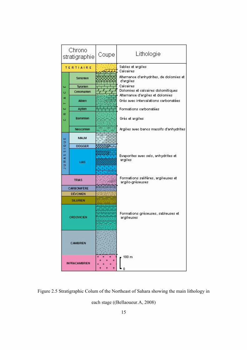
Figure 2.5 Stratigraphic Colum of the Northeast of Sahara showing the main lithology in
each stage ((Bellaoueur.A, 2008)

16
2.3 Local geological framework The exploration area is 4353.46KM2 and its surface altitude is about 230m. The surface
slope of the block dips down from west to east, the central and west area are dunes and
dune ridges, and the east is desert.
The seismic and drilling was started in 1970's. Now there are 7900km2 2D-seismic and
266km2 of 3D seismic data. Totally there are 62 wells drilled in this block, from among
them 20 are production wells. The oil fields were discovered between 1970 and 1984,
with a daily oil production of 624 m3/d (3925bbl/d).
According to the regional geological analysis and drilled formations in this basin the
strata sequence is Precambrian basement, Palaeozoic Cambrian (which is constituted by
one set of volcanic and meta sandstone with stable sedimentary facies), marine facies
sandstone and mudstone of Ordovician, clay shale of Silurian, sand-shale interbedding of
Devonian; sandstone/shale/gypsum-salt rock of Triassic in Mesozoic, gypsum-salt
rock/calcareous rock with shale of Jurassic, sandstone/calcareous rock/gypsum rock of
Cretaceous; the development of Cenozoic is not entire, it is mainly sand-mud rock of
Miocene and Pliocene of Tertiary. The main targets of exploration are Triassic, Devonian
and Ordovician.
The Triassic
It has been divided into 6 layers from bottom to top.
1. SI: interbedding of fine to medium sandstone with maroon and celadon
mudstone.

17
2. Volcanic effusive rock: andesite, basalt.
3. T1: consists of gray and maroon fine-to medium sandstone, its bottom
contains granules; the maroon barrier bed on its top is split from T2. It is the
production layer of this area.
4. T2: consists of brown and crimson-pearl silt and fine sandstone, its top is pelite
siltstone.
5. Argillaceous: mainly maroon mud stone.
6. S4: interbedding of white and pink salt rock with maroon and celadon mud
stone.
From the cross plane of well, the longitudinal distribution character of Triassic strata
shows the trend of gradually thickening from west to east, and sharply thinning from
south to north. The thickness of SI in Triassic changes between 12-96m, the northwest is
thicker than the southeast part and in the central part of this Block, the thickness
distribution is more stable, generally between 70-80m.The thicknesses of volcanic
effusive rock changes between 0-110m, its distribution characteristic shows that the
southern part is thicker than the northern part. The thickness of T1 in Triassic changes
between 0-78m, its northern thickness is larger than of the southern part. Note the
absence of T1 in well-4B and well-5. The thickness of T2 in Triassic changes between 9-
66m and its thickness distribution shows more stability in the central and the eastern area,
and it increases to northwest.

18
The thickness of the Devonian changes between 9-66m, and its thickness distribution
shows that the thickest part is located along the well-5 well-1Line and the strata sharply
thin down to the east.
2.4 The Geological Structure of the Study Area This block is geographically located in the north of OUED MYA Basin with more
flattening stratum and simple structure. Tectonically, this basin is located in the North
Africa platform. The structural system with SSW-NNE trend controls the areal structure
unit. Because of the Hercynian uplift, the strata of Paleozoic have been eroded. The
structure system trending SSW-NNE was formed by the Australian compression structure
movement in the end period of Lower Cretaceous. That movement controls the
distribution of structural traps. All the monoclines in this area are distributed from
Southwest to East North and show the complication caused by two set of fractures
trending in North East and East West.
Interpretation of 237 profiles indicated the existence of the structures below:
The top Triassic (S4), bottom Triassic (Hercynian surface SI), lower Ordovician (O).
32 traps have been discovered in this area, 27 traps confirmed and 5 new traps
discovered. The structural traps are mainly attached with fracture belt, and show the
distribution in form of pinch-and-swell. I list below some of the structures which are
traversed by wells.
Well-4 Structure
It is a fault anticline structure with drilling history. Its south and east regions are sheltered
by the normal faults trending NE and NW and the structure appears clearly on the 2D

19
seismic profiles LINE97-NGS-2 and LINE97-NGS-6. Now there are 11 controlled
survey lines, and 3 wells were drilled, out of which 2 wells have oil production history.
Well-5 Structure
It is an anticline structure with drilling history. Its east region is sheltered by a normal
fault trending NE; the axial direction is NE-SW and the structure is shown clear on the
2D seismic profiles LINE97-NGS-1 and LINE97-NGS-10. Now there are 14 controlled
survey lines, and 5 wells were drilled, 4 having oil production history.
Well-1B Structure
This trap is located to the south of Well-1B with distance of 2Km, its eastern region is
sheltered by the north south fault and its south is sheltered by the east fault, thereby it
forms a faulted anticline and its structural area is about 6.17Km2, the structural amplitude
closure is about 30ms two-way time.
2.5 Geological History of the Study Area
Sedimentary evolution of this area is a marine and continental facies. Sedimentary
association developed from Precambrian basement which consists mainly of volcanic
rocks and metamorphic quartz sandstone in Precambrian. This area was an open sea
deposition during Ordovician and Silurian periods, mainly developed marine facies
(quartz sandstone, mudstone and shale). Mudstone and shale developed from lower
Silurian is the main hydrocarbon source rock in this area. Sea water gradually shrunk
during Devonian period, developed a neritic shelf fades deposition; after that, the strata
uplifted and suffered from erosion due to Hercynian uplift. In Carboniferous, Permian,
this area integrally sank and undertook sedimentation, mainly of fluvial type. The

20
direction of main source material is SW—NE. The Devonian formation and overlying
Triassic formation present an unconformable contact.
2.6 The characteristics of the Source Rock The main source rock in the study area is the hot shale mudstone and shale in lower
Silurian. Its distribution keeps stable in the whole area, with a thickness of 40—60m .
Hot shale mudstone and shale (radioactive black shale) contain high abundance of
organic matter (TOC, generally about 4—10%). The kerogen is of type-2 which leads to
oil generation.
The lower Silurian clays are essentially grey to black clays, radioactive at the base. They
are present over the whole Saharan Platform. At a few places they have been removed
away by the Hercynian erosion phases (Figure 2.6a). The radioactive clays were
deposited immediately after the late Ordovician glacial period and correspond to the first
significant Paleozoic marine transgression. Radioactivity is mainly due to a high uranium
concentration. Thicknesses vary from 10 m to 100m with the maxima located in the
basins of Ahnet, Ghadames, Illizi, Oued Mya, Mouydir, to the north of Timimoun Basin
(Guern El Mor trough) and in the Benoud and Sbaa troughs (Figure 2.6 b). The total
organic carbon (TOC) varies from 1% to 11% but reaches 20% in some cases. The richest
zones are located in the vicinity of Hassi Rmel and Hassi Messaoud structures, in the
north-east of the Triassic province (El Borma and north of Ghadames Basin), to the west
of Illizi Basin, in the Sbaa trough and in the NE of the Grand Erg occidental. Organic
matter is of marine origin (algae, chitinozoa, graptolites; amorphous sapropelic organic
matter). The resulting source rock is of excellent quality and its hydrocarbon potential is
often in excess of 60 Kg HC/t as it is the case for the lower Silurian formations of the

21
Saharan Platform The separate evolution of each basin means that residual hydrocarbon
potentials vary from basin to basin. They are controlled by the state of maturation
reached in the radioactive clays. Kerogen maturation is the gas window (dry gas and
condensate) for the basins of Timimoun, Ahnet, Bechar and Mouydir, in the central and
northern parts of the Reggane and Tindouf Basins, in the centre of Ghadames Basin and
Oued Mya , and in the centre and the NW of the Sbaa trough. In other parts the same
kerogen is in the oil window, as in the rest of the Triassic province, in Illizi Basin, in the
south of the Reggane and Tindouf basins, in the east of Reggane in the vicinity of
Ougarta and finally in the SE of the Sbaa trough. In other cases the kerogen is not mature
(for example: in the south east of the Sbaa trough close to the Azzene uplift).
The mudstone and shale of the upper Ordovician is considered as a source rock for this
basin. Its organic matter content (TOC) is about 1-5%. The lower Ordovician (Shal
d’Azel and d’El Gassi) can also be considered as a source rock.

22
Basement Erosion Dry Gas Gas condensate Oil Mature zone
Figure 2.6 Maturation in the Lower Silurian Radioactive Clays (Geology of Algeria)

23
Figure 2.6 b.TOC Distribution in the Lower Silurian Radioactive Clays (Geology of
Algeria)
2.7 Sedimentary facies Analysis From bottom to top, sedimentary cap rock in this area is composed of deep, shallow
sea and continental facies strata. In Ordovician, marine sedimentary facies are mainly
quartz sandstone, mudstone and shale. Mudstone and shale are the main hydrocarbon
source rocks. The reservoir in this area is buried deeply and its porosity is low. Its
lithology is relative compact, so the effective reservoir storage place is formed only by
fractures. Lower Devonian (under Hercynian unconformity), is a neritic shelf fades
sedimentary, its thickness ranges from 0 to 239m. Reservoir lithology in the Devonian is
medium to fine grained sandstone, with porosity 4—20 % (average 12 %) and low
permeability is 0.03 — 100 md.

24
In Silurian, marine sedimentary facies mainly consist of a stable distribution of mud-
stone, dolomitic mudstone and argillaceous limestone.
In this area, Triassic is the main target layer and it is deposited in fluvial environment.
According to layer's color, depositional structure, lithology assembly and electrical
characteristics the classification can be as follows:
1. SI layer: It is mainly braided river sedimentation, it can be divided into over bank
deposit, channel bar sedimentary, fluvial-channel lag deposit.
2. T1, T2 layers: They are meandering river sedimentary, they can be divided to
point bar deposit, over bank deposit, crevasse splay deposit and fluvial-channel
lag deposit.
2.7.1 Fluvial-channel lag deposit It is medium to fine grained sandstone interbeded by argillaceous siltstone. Degree of
roundness is high. Gamma ray (GR) values range 20-160 API and resistivity response
shows large values, generally from 1 to 30Ω.m, resistivity curve appears as zigzag.
2.7.2 Point bar deposit It is meandering river sediments with medium to fine grained sandstone. The degree of
roundness is high. Gamma ray (GR) values range 30-50 API, resistivity value is low,
generally from 3 to 10Ω.m, resistivity curve is zigzag.
2.7.3 Channel bar sedimentary It is braided river sedimentation with medium to fine grained sandstone. The degree of
roundness is high. Gamma ray (GR) values range 20-40 API with high resistivity,
generally from 10 to 50Ω.m. Resistivity curve is shown as zigzag or bell shape. Sand
body maturity of this sedimentary micro-facies is high, this sedimentary formation is the

25
main reservoir.
2.7.4 Over bank deposit It is mudstone and silty mudstone, frequently has a massive structure, parallel and small-
sized cross bedding. Gamma ray (GR) values range 70-120 API with low resistivity
values, generally from 1 to 4Ωm. Resistivity curve is box shaped
2.7.5 Crevasse splay deposit It is an argillaceous siltstone, silty mudstone, with little sandstone at the bottom.
Frequently shows massive structure, sometimes shows parallel and small-sized cross
bedding. Gamma ray (GR) value is high, from 60 to 100 API with large resistivity values
range, generally from 2 to 100Ωm. Resistivity curve is dentate.
2.8 Reservoir Properties The main reservoirs (T1, TSI, Lower Devonian, Upper and Middle Ordovician ) with
their properties are summarized in the table below.

26
Table1.The main reservoirs in the study area and their properties.
Reservoir Thickness Lithology Porosity and Permeability
Triassic
T1,
sandstone <75
medium to
fine
sandstone
Φ: 2~17 % (average=10 %)
K: 0.1~300md (max500md)
TSI
Sandstone <95
coarse to
fine
Sandstone
Φ: 1~14 % (average= 8 %)
K: 0.04~200md(max800md)
Lower Devonian <240
medium to
fine
Sandstone
Φ: 4~20 % (average= 12
%)K:0.03~100md(max200md)
Upper Ordovician <20
Quartz
sandstone
Φ: 2~10 % (average= 6 %)
K: 0.02~3md(100md)
Middle Ordovician 150 Quartz
sandstone
Φ: 2~11 % (average= 7 %)
K: 0.03~8md(max200md)
27
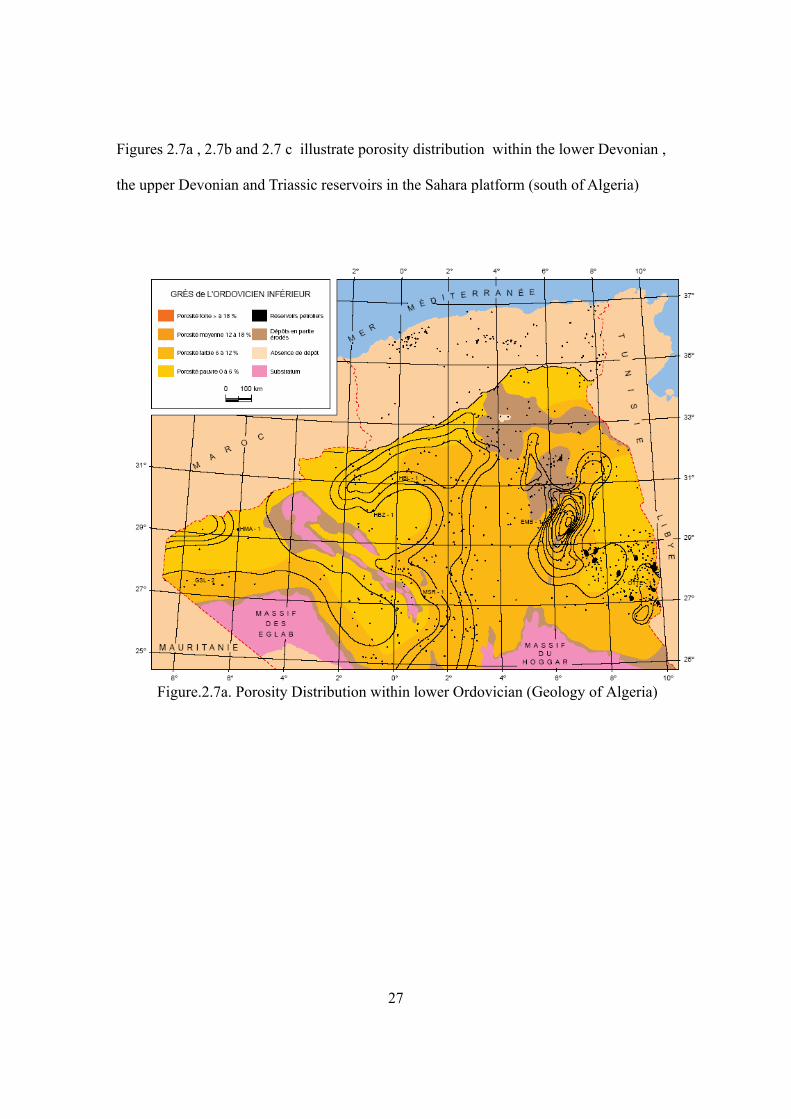
Figures 2.7a , 2.7b and 2.7 c illustrate porosity distribution within the lower Devonian ,
the upper Devonian and Triassic reservoirs in the Sahara platform (south of Algeria)
Figure.2.7a. Porosity Distribution within lower Ordovician (Geology of Algeria)

28
Figure 2.7 b. Porosity Distribution within upper Ordovician (Geology of Algeria)

29
Figure 2.7c. Porosity distribution within Triassic (Geology of Algeria)
The Triassic (TSi) sandstone lithology is fine to coarse grained sandstone and it is the
main production formation. TSi sand layer is the lower Triassic, the Hercynian erosion
plane landform controls Triassic Si sedimentary, it is the most favorable oil-gas
accumulation formation. Its main source material direction is SW—NE. The thickest of
TSi layers in this block is 95m, it is a braided river sedimentation formation with a net
thickness of sandstone generally 20-30m. TSi sandstone porosity is medium, with
medium pore size, permeability is not high but the existence of micro-fractures has made
a great improvement in reservoir properties, note ( Table.1) that the highest permeability
value is about 800mD.
Triassic T1: It is a meandering river deposit; its lithology is fine to medium grained

30
sandstone. T1 material source is from Hassi R’Mel ancient highland, with a thickness of
75m (the net thickness of the sandstone is 10-20m). The reservoir porosity is low to
medium with low permeability which was improved by the micro-fractures.
Devonian layer: This section is mainly shallow marine and continental shelf sediments.
It develops as offshore bar and underwater channel-mouth bar sand bodies. The oil
production from this reservoir is low.
Ordovician: Little oil and gas have been discovered in the northeast section of this area.
2.9 Cap rock characteristics The Mesozoic cap rocks correspond to the Triassic and Liassic clays and evaporites. In
the Triassic basin they act as cap rocks for the sandstone reservoirs and in some cases,
through an unconformity surface, for the Paleozoic reservoirs.
Due to their thickness, in excess of 2000 m, and their lithology they are classified as
"super seals". The cover consists of a number of sub-units. The "argillaceous Triassic" is
made of salty clays. Unit "S4" is a salty interval. The "argillaceous Liassic" is generally
overpressured. Unit "S3" is a Liassic interval, formed of salt and shale. It is followed by
units S1 and S2 which consist of salts, anhydrites and clays, topped by the Liassic B
dolomitic horizon and terminated by the upper Liassic anhydritic clays (Figure 2.8). Due
to pinchouts only the upper units are found on the borders of the Triassic basin. The
gypsum-salt rock of the Upper Triassic, the gypsum-salt rock, mud stone and limestone
of Jurassic-Cretaceous are good cap rocks in the study area.
The thickness of these rocks is up to 1000m.

31
Figure 2.8 . Distribution of Clay & Evaporate deposits from Triassic & Liassic (Geology of Algeria)
2.10 Migration System The oil and gas accumulation of this area has a direct relation with the Hercynian
unconformity plane and fault zone. The Hercynian movement in the Devonian caused an
erosion of the study area, and formed a local Hercynian unconformity plane.
Additionally, Australian structure movements formed a series of SSW – NNE direction
compresso-shear fault structural zones in early Cretaceous (Australia rifted away from
Africa), the long fracture extension and fault horizon reached Silurian, interconnected the
hydrocarbon source rock and overlaying sandstone rock reservoir.

32
CHAPTER THREE SEISMIC ATTRIBUTES CALCULATIONS AND ANALYSIS
3.1 Introduction
Seismic Reservoir Characterization (SRC) is a branch of Reservoir Geophysics, which
provides reservoir description using 2-D or 3-D seismic reflection methods. The main
objective of Seismic Reservoir Characterization is to predict and estimate reservoir
properties using 3-D seismic attributes as the main source of estimation of reservoir
parameters in the sparse inter-well area.
Generally, porosity, permeability, rock type, pore fluid, pore shape, burial depth
(temperature and pressure), consolidation (compaction and cementation) and geological
age are the most important rock properties to be considered in any description of the
reservoir. However, only some of these properties have a considerable effect on the
dominant component in the seismic response (namely: the velocity).
3.2 Definitions
Seismic attribute is any characteristics, qualitative or quantitative, measured,
calculated or inferred from seismic data, representing all the parameters of the trace
complex, geometrical configurations of seismic events and their spatial variations. Taner
et al. (1979) defined seismic attributes as all the information obtained from seismic data,
either by direct measurements or by logical or experience-based reasoning. They relate to
33
basic information from the seismic data, time, amplitude, frequency and attenuation. The
attributes provide alternative representations of seismic data and can be used for
geological and petrophysical characterization. These attributes can be classified in a way
that allows one to make the most of their usefulness in seismic.
Generally, the calculation of seismic attributes is based on data represented in time.
Therefore, conventional sections (CDP stack), the migrated sections before or after stack
are given as input for this calculation. The attributes derived from the migrated sections
in time, due to the accurate positioning of reflectors, may be more beneficial for the
objectives of the seismic interpretation.
Seismic attributes were introduced in the 1970's as useful tool to help interpret the
seismic data in a quantitative way. Walsh (1971) published the first paper under the title
of “Color Sonograms”. In the same period, Nigel Anstey published “Seiscom 1971” and
he introduced the concept of reflection strength and mean frequency. Realizing the
potential for extracting useful instantaneous information, Taner, Koehler and Anstey
turned their attention to wave propagation and simple harmonic motion (Taner, 2000).
Neidell proposed the use of the Hilbert transform to derive the kinetic portion of the
energy flux. In the mid 70’s three major attributes were established. Since the early
1990s, the quantitative analysis of seismic attributes has become widely used and applied
through calibration with well bore measurements (Doyen, 1988, Schultz et al.1994, Taner
et al.. 1994, Trappe and Hellmich, 1998).
In reservoir geophysics, rock physics play a role of a bridge establishing physical
relationships between seismic attributes and reservoir properties. Many examples are
found in literature related to seismic attributes and their application to reservoir

34
characterization;(Taner et al. 1979; Lawrence 1998; Brown 1999 and 2001; Skiruis
1999; Hampson et al. 2001).
3.4 Classification of Seismic Attributes
Chan and Sidney (1997) divided seismic attributes into two categories
Horizon based attributes
The average properties of the seismic trace are computed between two geologic
boundaries generally defined by picked horizons.
Sample based attributes
The input seismic traces are transformed in such a way as to produce a new output trace
with the same number of samples as the input (e.g., transformation of seismic amplitude
sample based volume to acoustic impedance sample based volume).
Post stack attributes can, therefore, be extracted along one horizon or over a specific
window (window attributes).
Taner et al. (1994) divided the attributes into two general categories
3.4.1 Geometrical attributes (reflection configuration)
They describe the spatial and temporal relationship of all other attributes. Lateral
continuity measured by semblance is a good indicator of bedding similarity as well as
discontinuity. Bedding dips and curvatures give depositional information. Geometrical
attributes are generally found useful in structural interpretation (e.g., faults) and in
seismic stratigraphic interpretation of 3D data volumes. Their objective is to enhance the

35
visibility of the geometrical characteristics of seismic events for the interpreter ( Taner
et al. 1994, 2000).
3.4.2 Physical attributes (reflection characteristics). They are related to physical qualities and quantities. The magnitude of the trace envelope
is proportional to the acoustic impedance contrast, frequencies are related to the bed
thickness, wave scattering and absorption. Instantaneous and average velocities are
directly related to rock properties. These attributes are mainly applicable for lithological
and reservoir characterization (Taner et al., 2000). They can be divided into two sets
• Attribute computed from seismic data planes (2-D planes): these attributes, computed
from analytical traces, are the most widely used ones. They include the trace envelope
and its first and second derivatives, instantaneous phase and instantaneous frequency,
instantaneous acceleration, apparent polarity, bandwidth, instantaneous Q factor
(attenuation), and their statistic computed along reflectors over a time window.
• Attributes computed from the pre-stack data: which reflect variation of various attributes
with offset, such as amplitude (AVO) and instantaneous frequency, ect. (Taner et al.,
1994).
3.4.3 Pre-stack Attributes: Seismic data are CDP or image gather traces.
They will have directional (azimuth) and offset related information. Computations
generate huge amounts of data; hence they are not practical for initial studies
(Taner, 2000).
3.4.4 Post stack Attributes: Stacking is an averaging process, losing offset and
azimuth information. Seismic data could be CDP stacked or migrated.
Based on the information content, attributes are divided into two groups (Taner, 2000).

36
3.4.5 Instantaneous Attributes:
Instantaneous attributes computed sample by sample, representing instantaneous
variations of different parameters. Instantaneous values of attributes such as trace
envelope, its derivatives, frequency and phase may be determined from the complex
trace.
3.4.6 Wavelet Attributes: Instantaneous attributes computed at the peak of the trace
envelope have a direct relation to the Fourier transform of the wavelet in the vicinity of
the envelope peak. For example, the instantaneous frequency at the peak of the envelope
is equal to the mean frequency of the wavelet amplitude spectrum.
Therefore, attributes can be divided into two sets based on their origin.
3.4.7 Reflection Attributes: They correspond to the characteristics of interfaces. All
instantaneous and wavelet attributes can be included under this category. Pre-
stack attributes such as AVO are also reflective attributes, since AVO analysis
measures the angle versus reflection response of an interface.
3.4.8 Transmissive Attributes: they are related to the characteristics of a bed between
interfaces. Q, absorption, dispersion, interval-, RMS- and average velocities
come under this category
37
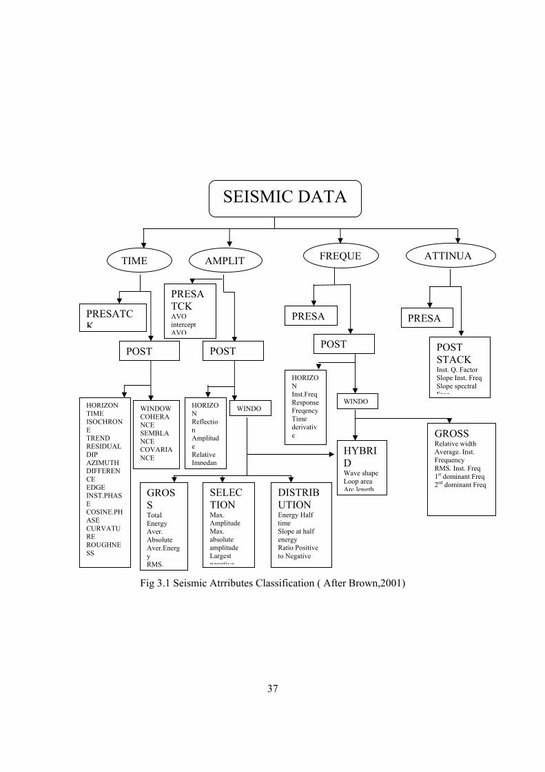
Fig 3.1 Seismic Atrributes Classification ( After Brown,2001)
SEISMIC DATA
POST STACK Inst. Q. Factor Slope Inst. Freq Slope spectral Freq
PRESAPRESATCK
POST
HORIZON TIME ISOCHRONE TREND RESIDUAL DIP AZIMUTH DIFFERENCE EDGE INST.PHASE COSINE.PHASE CURVATURE ROUGHNESS
WINDOW COHERANCE SEMBLANCE COVARIANCE
PRESATCK AVO intercept AVO
POST
GROSS Total Energy Aver. Absolute Aver.Energy RMS.
SELECTION Max. Amplitude Max. absolute amplitude Largest negative
DISTRIBUTION Energy Half time Slope at half energy Ratio Positive to Negative
HORIZON Reflection Amplitude Relative Impedan
WINDOWINDO
PRESA
POST
HORIZON Inst.Freq Response Freqency Time derivative GROSS
Relative width Average. Inst. Frequency RMS. Inst. Freq 1st dominant Freq 2nd dominant Freq
HYBRID Wave shape Loop area Arc length
TIME AMPLIT FREQUE ATTINUA
38
3.5 Hilbert Transform
Hilbert transform and analytical signal are useful for several applications in the field of
telecommunication and electronics. Hilbert transform has many seismic applications
such as:
• Introducing a phase shift.
• Measure of trace envelope.
• Measure of Instantaneous phase.
• Measure of Instantaneous frequency.
In seismic, these concepts are used to provide the local characteristics of a trace.
3.5.1 Definition of the Hilbert Transform
The Hilbert Transform of a function s(t) is given by:
=)(ˆ ts HT [ s(t) ] (3.1)
In the frequency domain HT defined by:
Sq(f)= FT[ )().()(ˆ fSfisignts −= (3.2)
In the time domain the transform is :
τττ
ππd
tsPv
tPptsts ∫
+∞
∞− −=∗=
)(111)()(ˆ (3.3)
Where Pv means Cauchy's principal value. Principal value integration is the limit of the
sum of two integrals from -∞ to -ε and from ε to +∞ as ε tends to zero.
PP: Principal part. The integration of the convolution is done as a principal value.

39
s(t) tV p
11π tVtsts p
11)()(ˆ π∗=
Figure 3.2 Hilbert Filter 3.5.2 Properties of Hilbert Transform
BEDROSIAN Theorem
Let s1(t) and s2(t) , two signals , the HT of their product is
HT [ s1(t) . s2(t) ] = [ ])()(1121 tststVp ⋅∗π
HT [ s1(t) . s2(t) ] ( ) )()(1121 tststVp ∗π= (3.4)
which enable us to write the following equality
HT[ s1(t) . s2(t) ] = s1(t) . HT [ s2(t) ] = HT [ s1(t) ] . s2(t) (3.5)
Orthogonality
The scalar product < s(t) , HT [ s(t) ] > is zero
Therefore,
< s(t) , )(ˆ ts > = ∫∫∞
∞−
∞
∞−
= dffSfSdttsts )(ˆ)()(ˆ)( (3.6)
with
FT [ t
PP1 ] = )sgn(fjπ−
40
So
)()sgn()(ˆ fSfjfS ⋅−=
The final result will be
∫∞
∞−
∧
=−=⟩⟨ 0)sgn()(, 2 dfffSjss (3.7)
Convolution
The HT of a convolution product is equal to the convolution product of one of the
signals with the HT of the other. If )()()()( 2121 fSfStsts ⋅↔∗
HT [ S1(f) . S2(f) ] = j sgn(-f) .[ S1(f) . S2(f) ]
= [ j sgn(-f) . S1(f) ] . S2(f)
= HT [ S1(f) ] . S2(f)
So
HT [ )()( 21 tsts ∗ ] = HT [ s1(t) ] ∗=∗ )()( 12 tsts HT [ s2(t) ] (3.8)
3.5.3 Discrete Hilbert Transform
The introduction of the discrete Hilbert transform makes possible the calculation of
analytical signal from sampled data, knowing that the majority of the data gathered for
processing, particularly in seismic, are in numerical form.
Given, the discrete sequence of complex numbers S (n), whose real part is indicated by
sr(n)), imaginary part by si(n) : sr(n) = Re [ s(n) ]
41
si(n) = Im [ s(n) ]
in the frequency domain the Fourier Transform is:
S(f)=Sr(f)+jSi(f) (3.9)
Fourier Transform causality is defined by:
⎪⎩
⎪⎨⎧
<≤−
≤≤=
0210
210)(
)(f
ffSfS
(3.10)
The conjugate of S(f) is given by:
)()()( fjSfSfS ir −−−=−
sr(n) is real so: Sr(-f) = Sr(f)
from equations (3.9) and (3.10) we get:
[ ])()(21)( fSfSfS r −+= (3.11)
And
[ ])()(21)( fSfSj
fS i −−= (3.12)
Following the property of causality of Fourier transform, a relation between the real and
imaginary parts can be established.
⎪⎩
⎪⎨⎧
<≤−−
≤≤=
021)(
210)(
)(2ffS
ffSfS r (3.13)

42
⎪⎩
⎪⎨⎧
<≤−−−
≤≤=
021)(
210)(
)(2ffS
ffSfjS i (3.14)
By comparing these two last expressions, the relation established is
⎪⎩
⎪⎨⎧
<≤
≤≤−=
021)(
210)(
)(ffjS
ffjSfS
r
ri
(3.15)
Or
Sr(f)=G(f).Si(f) (3.16)
with
⎪⎩
⎪⎨⎧
<≤−
≤≤−=
021
210
)(fj
fjfG
G (F) can be written in another form: G(f) = - jsgn(f) with f ≤ 21
g(n) = FT -1 [ G(f) ] = ∫+∞
∞−
πdfefG
fnj2)(
= ∫∫+
π
−
π−
21
0
20
21
2dfejdfej
fnjfnj
= ( )nn π−π cos11
= ( )2sin2 2 nn
ππ

43
Finally, the impulse response of Hilbert filter is given by
⎪⎩
⎪⎨⎧
=
≠=
00
0)2(sin2)(
2
n if
n if n
nng
ππ
Figure 3.3 Impulse Response of Hilbert Transform
0 1 2 3 4 5 6 7 8 9 10-2.5
-2
-1.5
-1
-0.5
0
0.5
1
1.5
2
2.5
Time (second)
Am
plitu
de
Impulse Response: blue. Ideal Response: red. Axis of symmetry: black

44
3.6 Computation of Seismic Attributes In this section several methods of analytic trace computation will be reviewed.
Frequency Domain Computation
The real and imaginary part of the analytical trace are Hilbert Transform pairs, then their
Fourier Transforms have to be causal, their amplitude spectra have to be the same and
their phase spectra have to be 90 degrees out of phase.
The analytical trace can be formed by the following steps:
• Transfer the seismic trace to a complex array and place it into the real part, leaving the
imaginary part equal to zero.
• Compute Fourier Transform by FFT.
• Zero out negative frequency, double the positive side, but leave zero and folding
frequencies as they are. This will create the causal Fourier Transform.
• The inverse Fourier Transform will give an input trace that is unaltered in the real part
and the imaginary part will contain the Hilbert Transform of the input trace.
Discrete Time Domain Computation
The discrete Hilbert Transform in the time domain is an infinitely long filter with zero
weights at the center and at all even-numbered samples. Its odd numbered coefficients are
1/n (Clearbout, 1976). In practice we use a limited-length filter which causes the
spectrum of the computed imaginary part to differ from that of the real part. The main
problem comes from phase discontinuities at zero samples. In order to overcome this, we
use a more convenient band-pass filter ( Butterworth).
Gabor-Morlet Decomposition
A major problem associated with the Hilbert Transform is that it is only valid for narrow-
band signals. For example, the spike has the widest possible bandwidth among all signals

45
and its Hilbert Transform is the time domain response of the transform. In the Gabor-
Morlet decomposition we divide the signal bandwidth into smaller Gabor-Morlet bands.
)exp().exp(),( 2 tittG ωαω −= (3.17)
The decomposition process is done by convolving the data by a series of Gabor-Morlet
wavelets. Since the wavelets are complex valued, their output will also be complex
valued and analytic.
3.6.1 Formulation of Seismic Attributes
Taner et al. (1979) gave the initial formulation of seismic attributes as applied to seismic
interpretation. His work covered five main attributes: envelope amplitude, instantaneous
phase, instantaneous frequency, weighted mean frequency and apparent polarity. Their
application was discussed by Robertson and Nogami (1984) for thin bed analysis, and
Robertson and Fisher (1988) for general interpretation.
In this section we will discuss the attributes computed directly from individual traces. We
will give the mathematical formulation of each attribute and indicate their direct or
possible relation to the physical properties of the subsurface.
(Amplitude/Trace) Envelope:
Let the analytical trace be given by
)()()( tihtstF += (3.18)
where
s(t): the real part corresponding to the seismic data.
h(t): the imaginary part corresponding to the Hilbert Transform of s(t).
The envelope is the modulus of the complex function F(t)

46
)()()( 22 thtstE += (3.19)
it represents the total energy, varies between 0 and the maximum amplitude of the trace.
The trace envelope is a physical attribute and it can be used as an indicator of the
following characteristics:
• Represents mainly the acoustic impedance contrast, hence reflectivity,
• Bright spots,
• Possible gas accumulation,
• Sequence boundaries,
• Unconformities,
• Major change in lithology,
• Major change in depositional environment,
• Lateral change indicating faulting,
• It has spatial correlation to porosity
Rate of Change of the Envelope
It shows the variation of the energy of the reflected events, it indicates the absorption
effects. A slower rise indicates larger absorption. The mathematical expression is given
by:
)(*)()]([ tdifftEdttEd = (3.20)
where
*: denotes convolution operation
diff: the differentiation operation.
47
This attribute has a concrete physical meaning and it can be used to detect possible
fracturing and absorption effects.
Instantaneous Phase
The argument of the complex analytic signal is the instantaneous phase
])()(arctan[)(
tsthtPh = (3.21)
The phase information is independent of trace amplitude and it relates to the propagation
phase of the seismic wave front. The instantaneous phase is also a physically meaningful
attribute and can be used for:
• To indicate lateral continuity,
• To compute the phase velocity,
• Has no amplitude information, hence all events are represented, even the weak ones
• Shows discontinuity, but may not be the best for this purpose
• Indicate sequence boundaries,
• Gives detailed visualization of bedding configurations,
• It is used to compute instantaneous frequency and acceleration
Instantaneous frequency
Represent the time rate of change of phase
ttxPhtxFreq
∂∂
=)],([),( (3.22)
Instantaneous frequency is a physical attribute; it can be used as effective discriminator in
case of lateral changes:
48
• Seismic character correlator in lateral direction,
• Indicates the edges of low impedance thin beds,
• Hydrocarbon indicator by low frequency anomaly,
• Fracture zone indicator, fractures may appear as lower frequency zones.
• Bed thickness indicator, high frequencies indicate sharp interface of thin shale bedding,
lower frequencies indicate sand-rich bedding.
• Sand /Shale ratio indicator in a clastic environment
Thin Bed Indicator
Information that can be extracted is the locations where instantaneous frequencies jump
or go in the reverse direction. These jumps are indicative of closely arriving reflected
wavelets. The thin-bed indicator is computed as the difference between the instantaneous-
and the time-averaged frequencies
)()()(. tttbedthin ωω −= (3.23)
This attribute is a physical attribute, it can be used for
• As an indicator of overlapping events,
• To indicate thin beds, when laterally continuous,
• To indicate non-reflecting zones, when they appear laterally random.
• Shows the fine details of bedding patterns.
Instantaneous Dominant Frequency
Similar to instantaneous frequency, it can be used as a reflection correlation tool.
49
Instantaneous Band Width
Related to overall absorption effects, considered as a high resolution seismic character
correlator tool.
Instantaneous Q Factor
It is a good indicator of absorption effects, fractures, gas zone and a possible permeability
indicator.
Normalized Amplitude
Useful for correlation , it is an event tracking tool and event termination indicator.
Dip of Maximum Coherency (a coherency attribute)
It is a good indicator for parallel, divergent or convergent bedding.
Apparent polarity
May differentiate between various types of bright spots, a section polarity indicator
Arc length
It measures reflection heterogeneity, and may be used to quantify lateral changes in
reflection patterns. It is calculated using the following formula:
ratesamplen
tjAmpjAmpZ
n
ij
×−
++−=∑−
=
)1(
)()1()((1
22
(3.24),
where Z is in milliseconds in time domain, or in feet or meters in depth domain.
Arc length is a stratigraphic sequence indicator.

50
Average energy
This is the squared RMS (Root Mean Square) Amplitude. This attribute is a measure of
reflectivity within a time or depth window and may be used to map direct hydrocarbon
indicators in a zone.
Average energy is computed using the following formula:
k
k
jAmpiAmp
k
i
k
j∑∑
=
=
⎟⎟⎟⎟⎟
⎠
⎞
⎜⎜⎜⎜⎜
⎝
⎛
⎟⎟⎟⎟⎟
⎠
⎞
⎜⎜⎜⎜⎜
⎝
⎛
−1
2
1)(
)(
(3.25)
assuming all samples are live samples.
Half energy
This operation computes the time or depth required for the cumulative energy within a
window to reach one-half of the total energy within the entire window. Half Energy is
computed by finding 2/1k from the following equation:
∑∑
∑∑
=
=
=
=
⎟⎟⎟⎟⎟
⎠
⎞
⎜⎜⎜⎜⎜
⎝
⎛
−=⎟⎟⎟⎟⎟
⎠
⎞
⎜⎜⎜⎜⎜
⎝
⎛
⎟⎟⎟⎟⎟
⎠
⎞
⎜⎜⎜⎜⎜
⎝
⎛
−
2/1
1
2
1
1
2
1
)()(
2
)()(
k
i
k
j
k
i
k
j
k
jAmpiAmp
k
jAmpiAmp
(3.26)
Half energy may indicate asymmetric changes in lithology or porosity within a specified
zone.

51
RMS Amplitude
RMS Amplitude is the square root of the sum of all squared amplitudes, divided by the
number of live samples as shown in the following formula:
2/1
1
2
1)(
)(
⎥⎥⎥⎥⎥⎥⎥⎥⎥⎥⎥
⎦
⎤
⎢⎢⎢⎢⎢⎢⎢⎢⎢⎢⎢
⎣
⎡
⎟⎟⎟⎟⎟
⎠
⎞
⎜⎜⎜⎜⎜
⎝
⎛
⎟⎟⎟⎟⎟
⎠
⎞
⎜⎜⎜⎜⎜
⎝
⎛
−∑∑
=
=
k
k
jAmpiAmp
n
i
k
j
(3.27)
Where n is number of all amplitudes, k is the number of live samples.
RMS may map directly to hydrocarbon indicators and other geologic features which
emerge from the background by their amplitude response. Additional discussion on
attribute categories and their relationships to reservoir properties are found in much
geophysical literature such as: Chen and Sidney (1997); Taner et al. (1979 & 2000) and
Brown (2001).

52
CHAPTER FOUR
Artificial Neural Networks
4.1 Definition
The Artificial Neural Network (ANN) is a processing paradigm imitating the way
biological nervous systems (eg: brain), process information, in other words, is an
emulation of a biological neural system. It is composed of a large number of
interconnected elements (neurons) working in parallel to solve specific problems. A
given ANN is configured for the specific application, such as pattern recognition or data
classification, through a learning process. Learning in biological systems involves
adjustments to the synaptic connections that exist between the neurons. This is true of
ANNs as well.
4.2 Historical background of Neural Networks
The history of neural networks can be divided into several periods:
4.2.1 First Period (Initial attempts)
In 1943, McCulloch and Pitts developed models of neural networks based on their
expertise in neurology. These models involved several assumptions about how neurons
worked. The networks were based on simple neurons which were considered to be binary
devices with fixed thresholds. The outputs of the models were simple logic functions
such as "A or B" and "A and B". An other attempt was made by using computer
simulations. In 1954, Farley and Clark (IBM researchers) maintained closed contact with
53
neuroscientists at McGill University. So whenever their models did not work, they
consulted the neuroscientists. This interaction established a multidisciplinary trend which
has continued to the present day.
4.2.3 Second Period (Promising & Emerging Technology)
Not only was neuroscience influential in the development of neural networks, but
psychologists and engineers also contributed to the progress of neural network
simulations. Rosenblatt (1958) stirred considerable interest and activity in the field when
he designed and developed the Perceptron. The Perceptron had three layers with the
middle layer known as the association layer. This system could learn to connect or
associate a given input to a random output unit. In 1960, Rosenblatt demonstrated the
Mark I Perceptron. The Mark I was the first machine that could “learn” to identify optical
patterns.
Another system was the ADALINE (Adaptive Linear Element) which was developed in
1960 by Widrow and Hoff (of Stanford University). The ADALINE was an analogue
electronic device made from simple components. The method used for learning was
different to that of the Perceptron, it employed the Least-Mean-Squares (LMS) learning
rule.
4.2.4 Third Period (Frustration & Disrepute)
In 1969, Minsky and Papert wrote a book in which they generalized the limitations of
single layer Perceptrons to multilayered systems. In the book they said: "...our intuitive
judgment that the extension (to multilayer systems) is sterile". The result of their book
54
was to eliminate funding for research with neural network simulations. As a result,
considerable prejudice against this field was created.
4.2.5 Fourth Period (Innovation)
Although public interest and available funding were minimal, several researchers
continued working to develop neuromorphically based computational methods for
problems such as pattern recognition. During this period several paradigms were
generated which modern work continues to enhance. Grossberg's (Steve Grossberg and
Gail Carpenter in 1988) influence founded a school of thought which explores resonating
algorithms. They developed the ART (Adaptive Resonance Theory) networks based on
biologically plausible models. Anderson and Kohonen developed associative techniques,
independently of each other. Klopf in 1972, developed a basis for learning in artificial
neurons based on a biological principle for neuronal learning called it heterostasis.
Werbos (1974) developed and used the back-propagation learning method, however
several years passed before this approach was popularized. Back-propagation nets are
probably the most well known and most widely applied of the neural networks today. In
essence, the back-propagation net is a Perceptron with multiple layers, a different
thershold function in the artificial neuron, and a more robust and capable learning rule.
Amari (A. Shun-Ichi, 1967) was involved with theoretical developments, he published a
paper which established a mathematical theory for a learning basis (error-correction
method) dealing with adaptive pattern classification. Fukushima (F. Kunihiko) developed
a step-wise trained multilayered neural network for interpretation of handwritten
characters. The original network was published in 1975 and was called the Cognitron.

55
4.2.6 Fifth Period (Re-Emergence)
Progress during the late 1970's and early 1980's was important for the re-emergence of
interest in neural networks. Several factors influenced this movement. For example,
comprehensive books and conferences provided a forum for people in diverse fields with
specialized technical languages, and the response to conferences and publications was
quite positive. The news media picked up on the increased activity and tutorials helped
disseminate the technology. Academic programs appeared and courses were introduced at
most major Universities (in US and Europe). In Europe, Japan and the US funding had
become available, and several new applications in industry and financial institutions
emerged.
4.2.7 Today
Significant progress has been made in the field of neural networks. Improvement beyond
current commercial applications appears to be possible, and research is advancing the
field on many fronts. Clearly, today is a period of transition for neural network
technology.
Why use neural networks
Neural networks, with their ability to derive meaning from complicated or imprecise data,
can be used to extract patterns and detect trends that are too complex to be noticed by
either humans or other computer techniques. A trained neural network can be thought of
as an "expert" in the category of information it has been trained to analyze. This expert
system can then be used to provide projections for new situations of interest and answer
"what if" questions.

56
Other advantages include:
a) Adaptive learning
An ability to learn how to do tasks based on the data given for training or initial
experience.
b) Self-Organization
An ANN can create its own organization or representation of the information it
receives during the learning time.
c) Real Time Operation
ANN computations may be carried out in parallel, and special hardware devices
are being designed and manufactured which take advantage of this capability.
d) Fault Tolerance via Redundant Information Coding
Partial destruction of a network leads to the corresponding degradation of
performance. However, some network capabilities may be retained even with
major network damage.
4.2 Comparison between Artificial neurons and Human neurons
Little information is available about how the human brain trains itself to process data. To
construct an artificial neural network, researchers imitated the individual cells that make
up of the brain rather than the whole brain which is enormously complicated. A neuron
cell, as seen in Figure (4.1) is the basic building block of the human brain. A typical
neuron collects signals from other neurons through a net of fine structures called
dendrites.
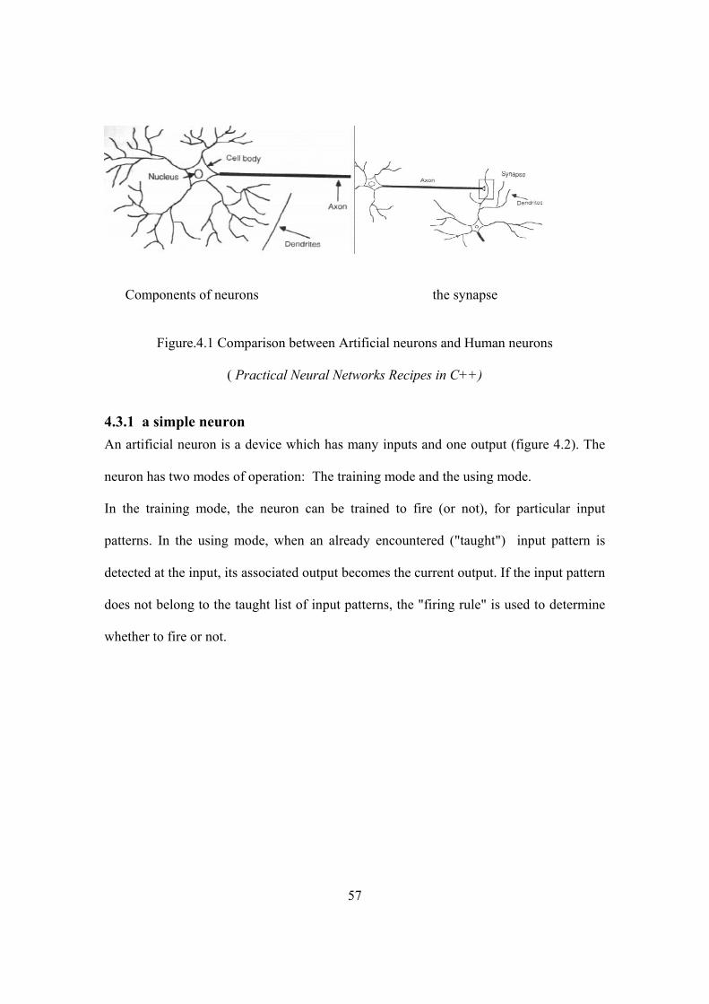
57
Components of neurons the synapse
Figure.4.1 Comparison between Artificial neurons and Human neurons
( Practical Neural Networks Recipes in C++)
4.3.1 a simple neuron An artificial neuron is a device which has many inputs and one output (figure 4.2). The
neuron has two modes of operation: The training mode and the using mode.
In the training mode, the neuron can be trained to fire (or not), for particular input
patterns. In the using mode, when an already encountered ("taught") input pattern is
detected at the input, its associated output becomes the current output. If the input pattern
does not belong to the taught list of input patterns, the "firing rule" is used to determine
whether to fire or not.
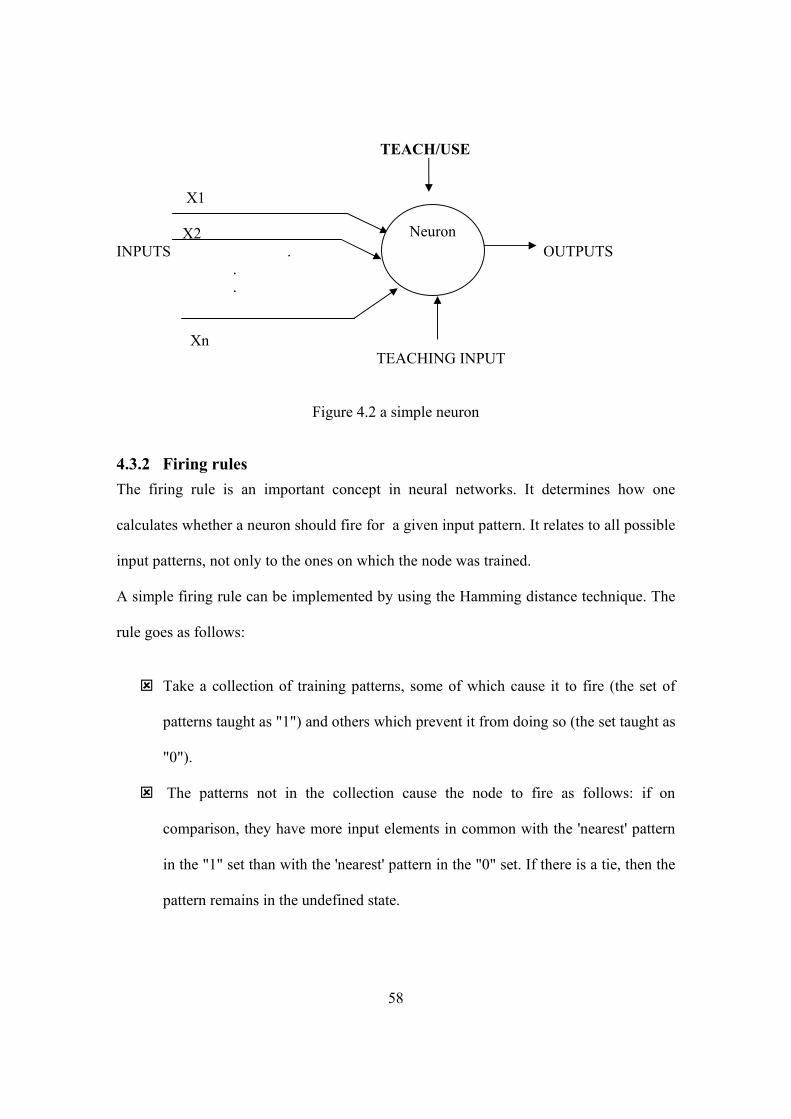
58
TEACH/USE
X1 X2 INPUTS . OUTPUTS . . Xn TEACHING INPUT
Figure 4.2 a simple neuron
4.3.2 Firing rules The firing rule is an important concept in neural networks. It determines how one
calculates whether a neuron should fire for a given input pattern. It relates to all possible
input patterns, not only to the ones on which the node was trained.
A simple firing rule can be implemented by using the Hamming distance technique. The
rule goes as follows:
Take a collection of training patterns, some of which cause it to fire (the set of
patterns taught as "1") and others which prevent it from doing so (the set taught as
"0").
The patterns not in the collection cause the node to fire as follows: if on
comparison, they have more input elements in common with the 'nearest' pattern
in the "1" set than with the 'nearest' pattern in the "0" set. If there is a tie, then the
pattern remains in the undefined state.
Neuron

59
Example:
A 3-input neuron is taught to produce output 1 when the input (X1, X2 and X3) is 111 or
101 and to output 0 when the input is 000 or 001. Then, before applying the firing rule,
the truth table is:
Table 2: The truth table
X1 0 0 0 0 1 1 1 1
X2 0 0 1 1 0 0 1 1
X3 0 1 0 1 0 1 0 1
output 0 0 0/1 0/1 0/1 1 0/1 1
4.3.3 How the firing rule works
Example 1:
Take the pattern 010. It differs:
from 000 in 1 element
from 001 in 2 elements
from 101 in 3 elements
from 111 in 2 elements.
Therefore, the 'nearest' pattern is 000 which belongs in the 0-taught set. Thus the firing
rule requires that the neuron should not fire when the input is 001.

60
Example 2:
The pattern 011 is equally distant from two taught patterns that have different outputs
and thus the output stays undefined (0/1).
By applying the firing rule, the truth table becomes
X1 0 0 0 0 1 1 1 1
X2 0 0 1 1 0 0 1 1
X3 0 1 0 1 0 1 0 1
output 0 0 0 0/1 0/1 1 1 1
Note : the difference between the two tables is called" the generalization of the
neuron".
4.4 Neural network structure
An artificial Neural Network is composed of several elements:
A - Input layer: the role of the input units is to receive the raw information that is fed into
the network.
B- Hidden layers: it is the processing unit for the network. Its activity is determined by
the activities of the input units and the weights of the connections between the input and
the first row of the hidden units, or between nodes of adjacent hidden layers.
C- Output layer: The behavior of the output units depends on the activity of the last row
of the hidden units and the weights between the nodes in this row and the output units.
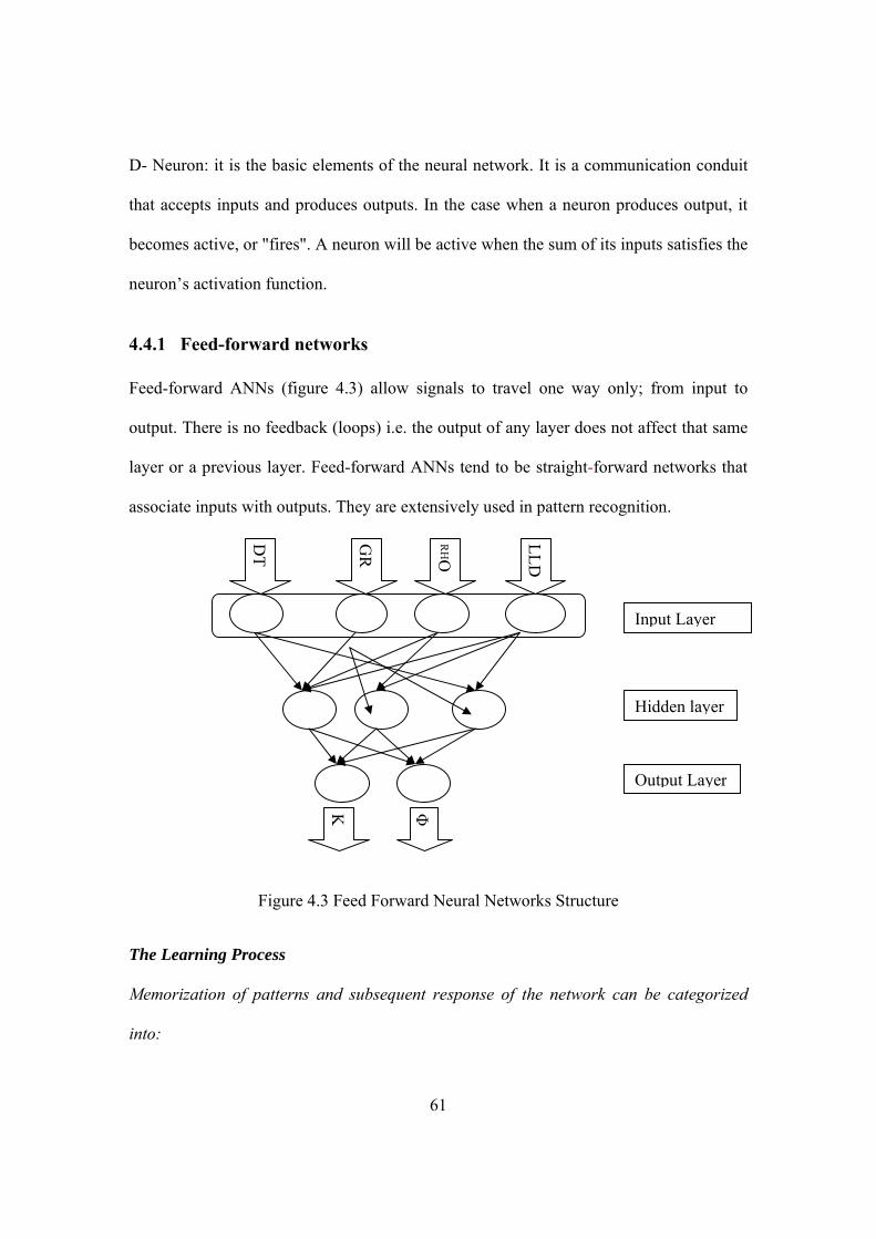
61
D- Neuron: it is the basic elements of the neural network. It is a communication conduit
that accepts inputs and produces outputs. In the case when a neuron produces output, it
becomes active, or "fires". A neuron will be active when the sum of its inputs satisfies the
neuron’s activation function.
4.4.1 Feed-forward networks
Feed-forward ANNs (figure 4.3) allow signals to travel one way only; from input to
output. There is no feedback (loops) i.e. the output of any layer does not affect that same
layer or a previous layer. Feed-forward ANNs tend to be straight-forward networks that
associate inputs with outputs. They are extensively used in pattern recognition.
Figure 4.3 Feed Forward Neural Networks Structure
The Learning Process
Memorization of patterns and subsequent response of the network can be categorized
into:
Input Layer
Hidden layer
Output Layer
DT
GR
RHO
LLD
K Φ

62
Associative mapping
In which the network learns to produce a particular pattern on the set of input units
whenever another particular pattern is applied on the set of input units. In associative
mapping the network stores the relationships among patterns. It can generally be broken
down into two mechanisms:
Auto association and hetero-association.
Regularity detection
In which the network learns to respond to particular properties of the input patterns. In
regularity detection the response of each unit has a particular 'meaning'. This type of
learning mechanism is essential for feature discovery and knowledge representation.
Notice that information is stored in the weight matrix of the neural network.
Following the way as the network learns we can distinguish between two types of neural
networks:
A- Fixed networks
In which the weights can not be changed( dW/dt=0). In such networks, the weights are
fixed a priori according to the problem to solve.
B- Adaptive networks
These are able to change their weights ( dW/dt ≠ 0).
4.4.2 Adaptive networks Adaptive means that the system parameters (Weights) are changed during operations.
This is called done during the training step. After the training phase the Artificial Neural

63
Network parameters are fixed and the system is deployed to solve the problem at hand
(the testing phase). Learning methods used in adaptive neural networks can be
categorized into two groups:
Supervised learning ( Figure 4.4)
Which incorporates an external teacher, the network is trained by providing it with input
and matching output patterns. During the learning process global information may be
required. Paradigms of supervised learning include error-correction learning,
reinforcement learning and stochastic learning. An important issue concerning supervised
learning is the problem of error convergence, the minimization of error between the
desired and computed unit values. The aim is to determine a set of weights which
minimizes the error. In one well-known method, which is commonly used for many
learning paradigms, the system converges to a set of weights providing the least mean
square (LMS) error.

64
Figure 4.4 Supervised Learning Scheme
Unsupervised learning
It is based upon only local information (no external teacher), it is also called Self
Organization, in the sense that it self-organizes the data presented to the network and
detects their emergent collective properties. In this paradigm the system is supposed to
discover statistically salient features of the input data. Unlike the supervised learning
process, there is no a priori set of categories into which the patterns are to be classified;
rather the system must develop its own representation of the input stimuli.
4.5 The Mathematical Model (figure 4.5) When we model a biological neuron, there are three important components:
1- The synapses of the neuron are modeled as weights. The strength of the
connection between an input and a neuron is given by the value of the weight.
+ -
Input Features
Neural Network
Target Features
Supervised Learning Algorithm
Weight/ threshold adjustment
Error vector
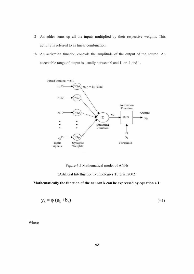
65
2- An adder sums up all the inputs multiplied by their respective weights. This
activity is referred to as linear combination.
3- An activation function controls the amplitude of the output of the neuron. An
acceptable range of output is usually between 0 and 1, or -1 and 1.
Figure 4.5 Mathematical model of ANNs
(Artificial Intelligence Technologies Tutorial 2002)
Mathematically the function of the neuron k can be expressed by equation 4.1:
yk = φ (uk +bk) (4.1) Where

66
∑=
=m
ijkju xwk
1 (4.2)
And where
xj is the input signal from an m dimensional input.
wkj is the synaptic weights of neuron k.
uk is the linear combiner output due to the input signals.
bk is the bias, )(⋅ϕ is the activation function.
yk is the output signal of the neuron.
The relation between the linear combiner output uk and the activation potential vk is
vk= uk +bk (4.3)
The activation function )(vϕ defines the output of a neuron in terms of the
induced local field v.
Activation Function
The behavior of an ANN (Artificial Neural Network) depends on the weights and the
input-output function (transfer function) that is specified for the units. This function
typically falls into one of three categories:
Linear: the output activity is proportional to the total weighted output. The
mathematic expression is y= ax, its graph is given in figure (4.6).

67
Figure 4.6 Purelinear function
Threshold Function (figure 4.7)
The output is set at one of two levels, depending on whether the total input is
greater than or less than some threshold value. The mathematical expression is
given by:
⎩⎨⎧
<≥
=0 00 1
)(vifvif
vφ
-5 -4 -3 -2 -1 0 1 2 3 4 5-5
-4
-3
-2
-1
0
1
2
3
4
5
x
y

68
-5 -4 -3 -2 -1 0 1 2 3 4 5-1
-0.8
-0.6
-0.4
-0.2
0
0.2
0.4
0.6
0.8
1
x
y
Figure 4.7 Threshold function
Sigmoid: the output varies continuously but not linearly as the input changes.
Notice that sigmoid units bear a greater resemblance to real neurons than do linear or
threshold units, but all three must be considered rough approximations. The mathematical
expression is given by
av-1
1)(e
v+
=φ
where a is the slope parameter of the sigmoid function. By varying the parameter a,
we can obtain sigmoid functions of different slopes.
A sigmoid graph is given in figure 4.8. For a =1.

69
Figure 4.8 Sigmoid Function
Tangent Hyperbolic Function
This transfer (activation) function is sometimes used in place of the sigmoid function and
is described by the following mathematical form
avav
avav
eeeevv −
−
+−
== )tanh()(φ
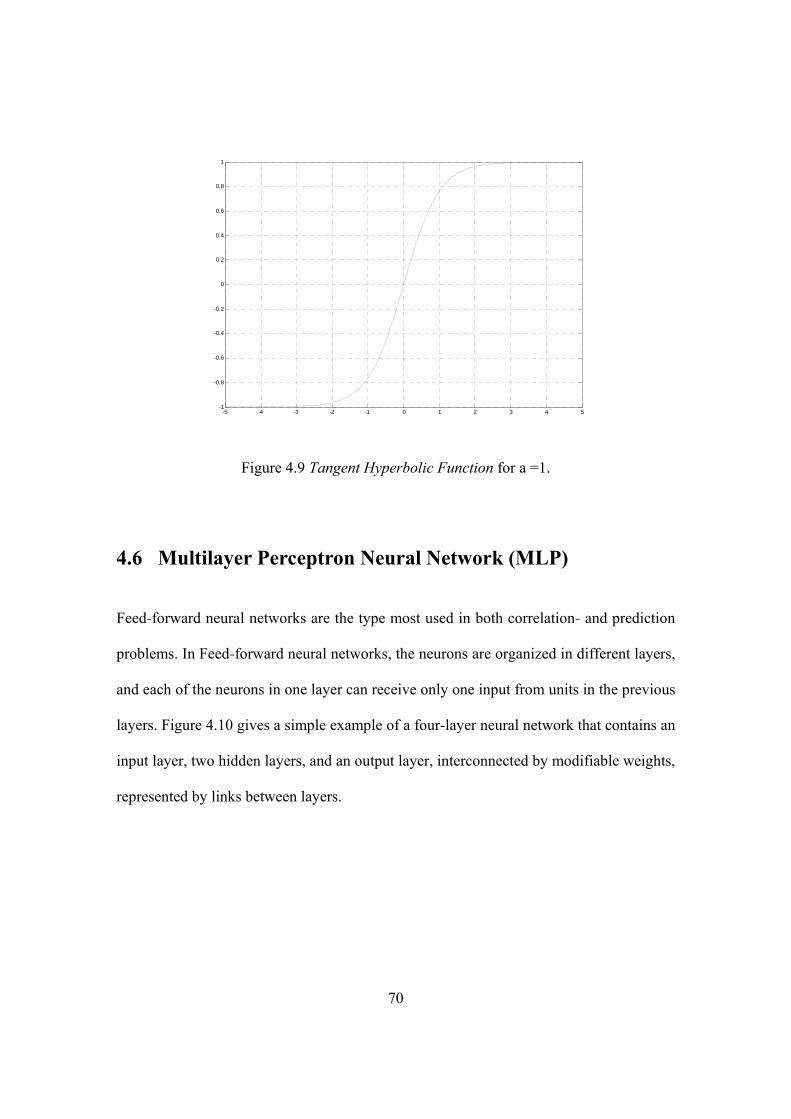
70
-5 -4 -3 -2 -1 0 1 2 3 4 5-1
-0.8
-0.6
-0.4
-0.2
0
0.2
0.4
0.6
0.8
1
Figure 4.9 Tangent Hyperbolic Function for a =1.
4.6 Multilayer Perceptron Neural Network (MLP) Feed-forward neural networks are the type most used in both correlation- and prediction
problems. In Feed-forward neural networks, the neurons are organized in different layers,
and each of the neurons in one layer can receive only one input from units in the previous
layers. Figure 4.10 gives a simple example of a four-layer neural network that contains an
input layer, two hidden layers, and an output layer, interconnected by modifiable weights,
represented by links between layers.

71
Figure 4.10: Multilayer Perceptron with two hidden layers (Artificial Intelligence
Technologies Tutorial 2002)
The presence of one or more hidden layers, whose neurons are correspondingly called
hidden neurons, enables the network to extract higher order statistics. Thus the network
acquires a global perspective, despite its local connectivity, by virtue of the extra set of
synaptic connections and the extra dimension of neural interaction. Such a network is
called a “multilayer feed-forward network”.
Learning Process of MLP
In the learning procedures one provides the network with a training set of patterns having
inputs and outputs. Real valued m–dimensional input feature vectors
(x1 ,x2,…xn) are presented to each of the first hidden layer units through the weight vector
w. Hidden layer unit k receives input j through the synaptic weight wkj ⎩⎨⎧
==
mjnk
,........,2,1,.......,2,1
.

72
Unit k computes a function of the input signal x and the weights wkj and then it passes its
output forward to all of the units in the next successive layer. Like the first hidden layer,
the units of the second hidden layer are fully connected to the previous layer through the
synaptic weights. These units also compute a function of their inputs and their synaptic
weight and they pass their output on to the next layer. The output of one layer becomes
the input to the following layer. Then, at the output, the unit error is calculated between
the target value and the computed value of the pattern. This process is repeated until the
final computation is produced by the output unit. The learning algorithm for this type of
network is called the back propagation (BP) algorithm, and it was published in the mid-
1980s for multilayer perceptrons. This architecture of the network is the basic unit in the
present study. Hornik et al. (1989) suggested that, if a sufficient number of hidden units
are available, then an MLP with one hidden layer and a sigmoid transfer function in the
hidden layer and a linear transfer function in the output layer can approximate any
function to any degree of accuracy.
Back-propagation is a reliable method for training multilayer neural networks due to its
strong mathematical foundation. Despite its limitations, back-propagation has
dramatically expanded the range of problems we can solve by ANN's. Many successful
implementations demonstrate its power. The steps to implement the back-propagation
algorithm are as follows: The error signal at the output of neuron j at iteration n (i.e.
presentation of the nth training pattern) is defined by
Ej(n)=dj(n)-yj(n) (4.4)
where dj(n) is the desired response for neuron j
yj(n) is the function signal appearing at the output of neuron j

73
Ej(n) refers to the error signal at the output of neuron j.
The instantaneous value of the sum of squared errors is obtained by summing the
sum of squared errors over all neurons in the output layer; as
∑∈
=cj
j ne )(21 2ξ (4.5)
The net internal activity level vj(n) produced at the of neuron j is therefore written as
)()(0
nynwv i
p
ijij ∑
=
= (4.6)
where p is the total number of inputs applied to neuron j and wji(n) denote the synaptic
weight connecting the output of neuron i to the input of neuron j at iteration n. Hence the
output of neuron j at iteration n is given as
Yi(n)= φj(vj(n)) (4.7)
The instantaneous gradient which is proportional to the weight correction term is
given as
)()()()()()()()(
)()(
nwnvnynenvnynen
nwn
jijjj
jjj
ji ∂∂∂∂∂∂∂∂
=∂∂ ξξ
)())(()()()( ' nynvne
nwn
jjjj
ji
φξ−=
∂∂
(4.8)
The correction Δwji (n) applied to wji(n) is defined by the delta rule as

74
))(()()()()()(
)()()(
' nvnennynnw
nwnnw
jjjj
ijji
ji
ji
φδηδ
ξη
=
=Δ
∂∂
=Δ
(4.9)
η is a small constant called Learning rate, it determines to what extent the newly
acquired information will override the old ones.
When neuron j is located in a hidden layer of the network, the local gradient is redefined
as
)())(()(
))(()()()(
'
'
nwnvn
nvnynn
kjk kjjj
jj
j
j
∑=
∂∂
=
δφδ
φξδ (4.10)
where computation of δk requires the knowledge of the error signals ek for all those
neurons that lie in the layer to the immediate right of hidden neuron j. The wkj(n) consists
of the synaptic weights associated with these connections. We are now ready to carry out
the weight correction update for the back-propagation algorithm, which is defined by the
delta rule
jjji ynw ηδ=Δ )( (4.11)
Note: the weight correction term depends on whether neuron j is an output node or a
hidden node:
if neuron j is an output node, equation 4.10 is used for the computation of the
local gradient.

75
if neuron j is a hidden node, equation 3.11 is used for the computation of the local
gradients.
4.6.1 The Network Performance The network performance is checked by monitoring the mean square error. The mean
squared error is obtained by summing ξ (n) over all n and then normalizing with respect
to N (number of training patterns)
∑=
=N
nAv nN 1
)(1 ξξ (4.12)
The process is repeated several times for each pattern in the training set, until the total
output squared error converges to a minimum, or until some preset limit is reached in the
number of training iterations.
One of the major problems with the back propagation algorithm is the long training times
due to the steepest descent method of optimization (minimization), which is
algorithmically simple but slow. The learning rate is sensitive to the weight changes. The
smaller the learning rate, the smaller will be the changes to the synaptic weights from one
iteration to the next, and the smoother will be the trajectory in the weight space.
However, if the learning rate is chosen too large in order to speed up the learning process,
the resulting large changes in the synaptic weights make the network unstable. The
solution for this problem is to add a momentum term to the weight update in the back
propagation algorithm.
Momentum term is simple to implement, and it significantly increases the speed of
convergence. The inclusion of the momentum term may also have the benefit of

76
preventing the learning process from terminating in shallow local minima on the error
surface.
An other method of accelerating the back propagation algorithm is achieved by using the
Levenberg - Marquardt algorithm (Hagan et al., 1996). It is based on Newton’s
optimization method (Hagan et al., 1996) and differs from the usual back propagation
algorithm in the manner in which the resulting derivatives are used to update the weights.
The main drawback of the LMBP (Levenberg - Marquardt Back Propagation) algorithm
is the need for large memory and storage space of the free parameters in the computers. If
the network has more than a few thousand parameters, the algorithm becomes impractical
on current machines.
4.6.2 Testing (Generalizing) A network is said to generalize well when the input-output mapping computed by the
network is correct for test data which is unknown to the network. A well designed neural
network will produce a correct output mapping, even when the input is slightly different
from the data used for training. However, when a neural network has too many neurons
in the hidden layers, the network may end up memorizing the training data. It even find
some irrelevant feature that is present in the training data (noise) but not a real property
of the underlying function that is to be modeled. This phenomenon is referred to as
overfitting. Overfitting is the result of more hidden neurons than actually necessary, with
the result that undesired contributions in the input space due to noise, spurious
periodicities, etc. are stored in the synaptic weights.

77
On the other hand if the number of hidden neurons is less than the optimum number, then
the network is unable to learn the correct input-output mapping. Therefore, it is important
to determine the optimum number of hidden neurons for a given problem.
Testing is influenced by three factors (Haykin, 1999)
the size of the training set.
the architecture of the neural network.
the complexity of the problem.
4.6.3 Advantages and disadvantages of MLP
An MLP network generates a nonlinear relationship between inputs and outputs by
interconnecting nonlinear neurons. The nonlinearity is distributed throughout the
network. It does not require any assumption about the underlying data distribution for
designing the networks. The network exhibits a great degree of robustness or fault
tolerance because of its built-in redundancy. Damage to a few nodes or links thus need
not impair overall performance significantly. It can form in any unbounded decision
region in the space spanned by the inputs. Such regions include convex polygons and
unbounded convex regions. The network has a strong capability for function
approximation. The abilities to learn and generalize are additional qualities. Previous
knowledge of the relationship between input and output is not necessary, unlike for
statistical methods. The MLP has a built-in capability to adapt its synaptic weights to
changes in the surrounding environment by adjusting the weights to minimize the error.
Experience with neural networks has revealed a number of drawbacks for the technique.
For an MLP network, the, i.e. the number of hidden layers and neurons, the size of the

78
training dataset, and the type of transfer function(s) for neurons in the various layers are
all important for the solution of a given problem,. With no analytical guidance on the
choice of the design parameters (initial weights, learning rate, and momentum), the
developer has to follow an ad hoc, trial-and-error approach of manual exploration.
Although acceptable results may be obtained with some effort, it is obvious that
potentially superior models might be easily overlooked. The considerable amount of user
intervention not only slows down model development, but also works against the
principle of ‘letting the data speak’, i.e. objectivity. Over-fitting or poor network
generalization with new data during actual use is another problem. The commonly used
back-propagation training algorithm, with a gradient descent approach to minimize the
error during training, suffers from the local minima problem, which may prevent to arrive
at the optimum model.
Another problem is the black-box nature of neural network models. The lack of
explanation capabilities is a handicap in many decision support applications such as
medical diagnostics, where the user would naturally like to know how the model has
come to a certain conclusion. Model parameters are buried in large weight matrices,
making it difficult to gain insight into the modeled phenomenon or compare the model
with available empirical or theoretical models. Information on the relative importance of
the various inputs to the model is not readily available, which hampers efforts for model
reduction by discarding less significant inputs. Additional processing, using techniques
such as the principal component analysis, may be required for this purpose.

79
4.7 General Regression Neural Networks In 1990, Donald F. Specht formulated the weighted-neighbor method in the form of a
neural network. He called this a Probabilistic Neural Network. Here is a diagram of a
GRNN network
Figure.4.11 Typical GRNN architecture
All GRNN networks have four layers:
Input layer ( Input nodes)
There is one neuron in the input layer for each predictor variable. The input
neurons (or pre-processing before the input layer) standardize the range of the values
by subtracting the median and dividing by the interquartile range. The input neurons
then feed the values to each of the neurons in the hidden layer.
X1
X2
X3
H1
H1
H1
H1
C1
C2
Z
Input nodes
Hidden nodes
Class nodes
Decision nodes
80
Hidden layer ( Hidden nodes)
This layer has one neuron for each case in the training data set. The neuron stores
the values of the predictor variables for the case along with the target value. When
presented with the x vector of input values from the input layer, a hidden neuron
computes the Euclidean distance of the test case from the neuron‘s center point and
then applies the RBF (Radial Basis Function) kernel function using the sigma
value(s). The resulting value is passed to the neurons in the pattern layer.
Pattern layer ( Class nodes)
This layer has one neuron for each case in the training data set. The neuron stores the
values of the predictor variables for the case along with the target value. When presented
with the x vector of input values from the input layer, a pattern neuron computes the
Euclidean distance of the test case from the neuron’s center point, and a radial basis
function (RBF) (also called a "kernel function") is applied to the distance to compute the
weight (influence) for each point,
Weight = RBF (distance) (equation 4.13).
The calculations performed in each pattern neuron of GRNN are exp(-D2/2σ2) with the
normal distribution centered at each training sample. The radial basis function is so
named because the radial distance is the argument to the function. The further some other
point is from the new point, the less influence it has. Different types of radial basis
functions can be used, but the most common is the Gaussian function (figures 4.12
&4.13). The peak of the radial basis function is always centered on the point it is
weighting. The function’s sigma value (σ) determines the spread of the RBF function;
that is, how quickly the function declines as the distance increases from the point. With

81
larger sigma values and more spread, distant points have a greater influence. Then the
resulting value is passed to the neurons in the summation layer.
Summation layer
There are only two neurons in the summation layer. One is the denominator
summation unit, the other numerator summation unit. The denominator summation unit
adds up the weight values coming from each of the hidden neurons. The numerator
summation unit adds up the weight values multiplied by the actual target value for each
hidden neuron.
Decision layer ( Decision nodes)
The decision layer divides the value accumulated in the numerator summation unit
by the value in the denominator summation unit, and it uses the result as the predicted
target value.
Figure.4.12 Radial Basis Transfer Function for one input

82
Figure.4.13 Radial Basis Transfer Function for multi inputs
The main consideration when training a GRNN network is the proper selection of the
optimal sigma values to control the spread of the RBF functions.
)()(
)2/exp()2/exp(
)(
2
1
22
1
22
i
T
ii
n
i i
n
i ii
xxxxD
DDy
xY
−−=
−
−=
∑
∑
=
=
σσ
(4.13)

83
4.7.1 Advantages and disadvantages of GRNN GRNN networks have advantages and disadvantages compared to multilayer
perceptron networks:
It is usually much faster to train a GRNN network than an MLP network.
GRNN networks are often more accurate than MLP networks.
GRNN networks are relatively insensitive to outliers
GRNN networks are slower than MLP networks at classifying new cases.
GRNN networks require more memory space.

84
CHAPTER FIVE
PERFORMANCE ANALYSIS AND COMPARATIVE STUDIES
5.1 Overview The main contribution of this Thesis is to investigate and develop neural network
models for porosity, permeability and lithofacies estimation using Multilayer Perception
Neural Network and General Regression Neural Network.
In the first part of this chapter, I present the implementation process for estimation of
porosity, permeability and lithofacies from well logs based on the framework discussed
in Chapter 4. The results to be presented have been obtained from the implementation of
Multilayer Perception Neural Network (MLP) and General Regression Neural Networks
(GRNN).
In the second part, I present the estimation of reservoir properties (porosity, permeability
and lithofacies) from Seismic Attributes. Only those results will be presented which
were obtained using General Regression Neural Network (GRNN).
In the third part, integration of well logs and seismic attributes will be used to predict
porosity, permeability and lithofacies as a function of depth.
In the last part of the Thesis, I present the spatial prediction of these properties. The
Neural Network Model used for this purpose was built using the professional software
“Petrel” of Sclumberger.

85
5.2 DATA ANALYSIS
In this study I used a data set from a Reservoir in South Algeria. The data consist of
well logs, core porosity values, core permeability values and data of a 3-D seismic
survey. The study area has seven wells from which 3 wells have core data. In this work
we used two wells named Well-1 , Well-2 with a total of 145 data samples. I investigated
these data sets, and performed statistical analysis to determine the hidden patterns and
deterministic relationship between the actual outputs and the provided input features.
This helps to get more knowledge about the data. The two wells were combined together
and divided randomly into two sets, namely the training and testing sets of 70% and 30%
respectively. The training set was then used to build the model while the testing set was
used to evaluate the predictive power of the model. In order to study the prediction of
porosity and permeability six well logs namely; Sonic log (DT), Neutron log (NPHI),
Density log (RHOB), Gamma Ray (GR), Deep Resistivity (LLD), and Shale Volume
(Vsh) were used as inputs to both networks.
To determine the performance and accuracy of the models, I made use of some of the
statistical quality measures, namely: correlation coefficient, and root mean squared error.
A good model should have a high correlation coefficient (CC) and a low root mean
square error (RMSE).
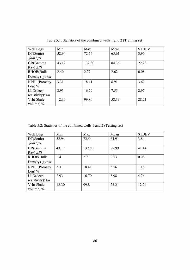
86
Table 5.1: Statistics of the combined wells 1 and 2 (Training set)
Well Logs Min Max Mean STDEV DT(Sonic)
sfoot μ/ 52.94 72.54 65.61 3.96
GR(Gamma Ray) API
43.12 132.80 84.36 22.23
RHOB(Bulk Density) 3/ cmg
2.40 2.77 2.62 0.08
NPHI (Porosity Log) %
3.31 18.41 8.91 3.67
LLD(deep resistivity) mΩ
2.93 16.79 7.55 2.97
Vsh( Shale volume) %
12.30 99.80 58.19 28.21
Table 5.2: Statistics of the combined wells 1 and 2 (Testing set)
Well Logs Min Max Mean STDEV DT(Sonic)
sfoot μ/ 52.94 72.54 64.91 3.84
GR(Gamma Ray) API
43.12 132.80 87.99 41.44
RHOB(Bulk Density) 3/ cmg
2.41 2.77 2.53 0.08
NPHI (Porosity Log) %
3.31 18.41 5.56 1.18
LLD(deep resistivity) mΩ
2.93 16.79 6.98 4.76
Vsh( Shale volume) %
12.30 99.8 23.21 12.24

87
5.3 Experimental Results Using Mutilayer Perception and General Regression Neural Networks An MLP model was developed to estimate porosity and permeability along the vertical
axis using well log data. Different models were tried before selecting the best one. The
best model had one input layer with six neurons, two hidden layers with twenty neurons
(ten for each) and one output layer. Purely linear and sigmoidal functions were used as
activation functions for this model.
5.3.1 Porosity Estimation Results From Well Logs The MLP model is able to predict porosity, with a correlation coefficient
CC=0.91 and MSE=0.10 for the training set, but CC = 0.66 and MSE= 0.40 for
the testing set. The results for the estimation are shown in Table 4.3, while
Figures 4.1a and 4.1b show the performance plot for the best selected model.
The GRNN model was built to predict porosity, using the following
parameters: The apropriete sigma (0.01-50) for each variable and the Gaussian
as kernel function. The results provided by GRNN were for the training process
CC=0.97 and MSE =0.07, while for the testing process CC=0.81 and MSE=0.37.
Figures 4.2a and 4.2b show the performance plot for the best selected model.

88
Figure 5.1a Training core porosity vs predicted porosity using MLP
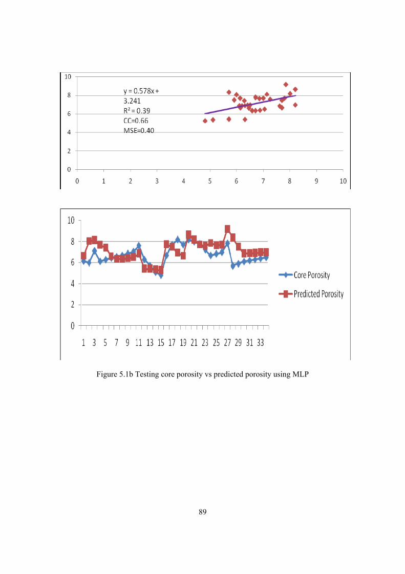
89
Figure 5.1b Testing core porosity vs predicted porosity using MLP

90
Figure 5.2a Training core porosity vs predicted porosity using GRNN

91
Figure 5.2b Testing core porosity vs predicted porosity using GRNN
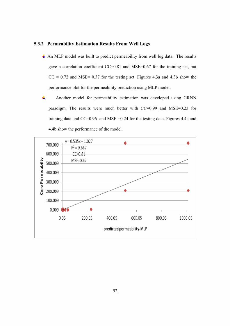
92
5.3.2 Permeability Estimation Results From Well Logs
An MLP model was built to predict permeability from well log data. The results
gave a correlation coefficient CC=0.81 and MSE=0.67 for the training set, but
CC = 0.72 and MSE= 0.37 for the testing set. Figures 4.3a and 4.3b show the
performance plot for the permeability prediction using MLP model.
Another model for permeability estimation was developed using GRNN
paradigm. The results were much better with CC=0.99 and MSE=0.23 for
training data and CC=0.96 and MSE =0.24 for the testing data. Figures 4.4a and
4.4b show the performance of the model.

93
Figure 5.3a Training core permeability vs predicted permeability using MLP
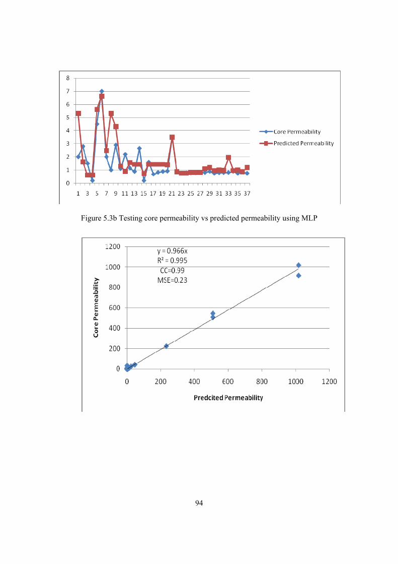
94
Figure 5.3b Testing core permeability vs predicted permeability using MLP
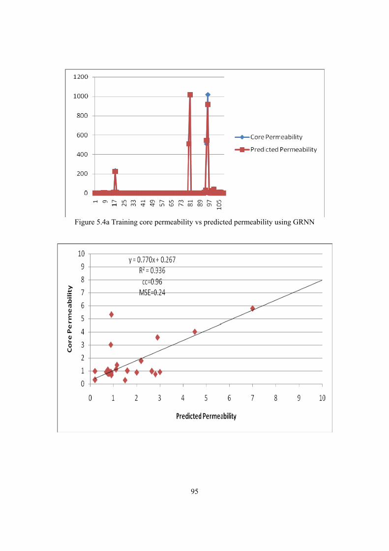
95
Figure 5.4a Training core permeability vs predicted permeability using GRNN

96
Figure 5.4b Testing core permeability vs predicted permeability using GRNN
Table 5.3 Results Summary for MLP and GRNN models
Type of Paradigm Porosity Permeability
Multilayer Perceptron Neural Network
Training (CC=0.91& MSE=0.10)
Testing (CC=0.66 &
MSE=0.40 )
Training (CC=0.81 & MSE=0.67)
Testing (CC=0.72 &
MSE=0.37 )General Regression Neural
Network Training (CC=0.97 &
MSE=0.67 )
Testing (CC=0.81& MSE=0.37 )
Training (CC=0.99 & MSE=0.23)
Testing (CC=0.96 &
MSE=0.24)
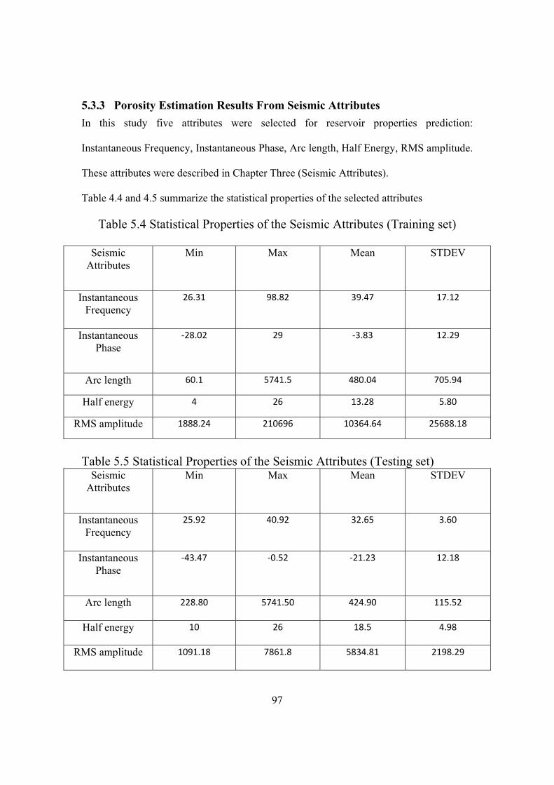
97
5.3.3 Porosity Estimation Results From Seismic Attributes In this study five attributes were selected for reservoir properties prediction:
Instantaneous Frequency, Instantaneous Phase, Arc length, Half Energy, RMS amplitude.
These attributes were described in Chapter Three (Seismic Attributes).
Table 4.4 and 4.5 summarize the statistical properties of the selected attributes
Table 5.4 Statistical Properties of the Seismic Attributes (Training set)
Seismic Attributes
Min Max Mean STDEV
Instantaneous Frequency
26.31 98.82 39.47 17.12
Instantaneous Phase
‐28.02 29 ‐3.83 12.29
Arc length 60.1 5741.5 480.04 705.94
Half energy 4 26 13.28 5.80
RMS amplitude 1888.24 210696 10364.64 25688.18
Table 5.5 Statistical Properties of the Seismic Attributes (Testing set)
Seismic Attributes
Min Max Mean STDEV
Instantaneous Frequency
25.92
40.92
32.65
3.60
Instantaneous Phase
‐43.47
‐0.52
‐21.23
12.18
Arc length 228.80
5741.50 424.90
115.52
Half energy 10
26
18.5
4.98
RMS amplitude 1091.18
7861.8
5834.81
2198.29

98
Note: For GRNN and MLP models using Seismic Attributes I used the two wells, and
extracted the seismic attributes at the well location ("Well Seismic"). I took as a reference
the top of the reservoir and calculated the attributes at every two millisecond (sample
rate =2 ms) for the total depth of 80ms ( TWT) in each well.
Figures 4.5 and 4.6 show the base map and the 3-D seismic volume for the study site in
which it indicates the location of the main wells drilled in this area. Figure 4.7 illustrate
the top of the reservoir T1.
Figure 5.5 Base map of the study area

99
Figure 5.6 3D Seismic Volume of the study site
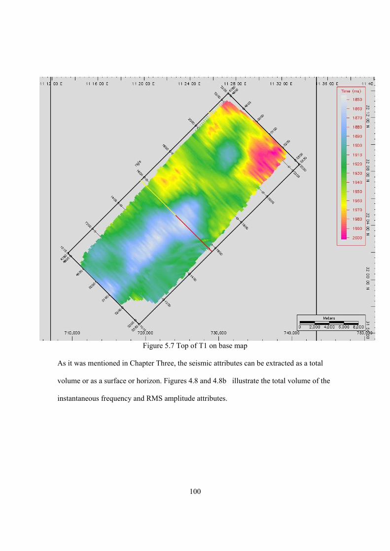
100
Figure 5.7 Top of T1 on base map
As it was mentioned in Chapter Three, the seismic attributes can be extracted as a total
volume or as a surface or horizon. Figures 4.8 and 4.8b illustrate the total volume of the
instantaneous frequency and RMS amplitude attributes.

101
Figure 5.8a 3D Volume of Instantaneous Frequency

102
Figure 5.8b 3D Volume of RMS amplitude
From these volumes surface or horizon attributes can be extracted. Figures 4.9a, 4.9b,
4.9c, 4.9d show the time-slice attributes (Instantaneous Frequency) at different levels
(2ms,8ms,12ms,20ms), while figures 4.10a, 4.10b, 4.10c, 4.10d show the time slice of
( Instantaneous Phase ) at ( 2ms,6ms,10ms,12ms).

103
Figure 5.9a Time slice of the Instantaneous Frequency at 2ms
Figure 5.9b Time slice of the Instantaneous Frequency at 8ms
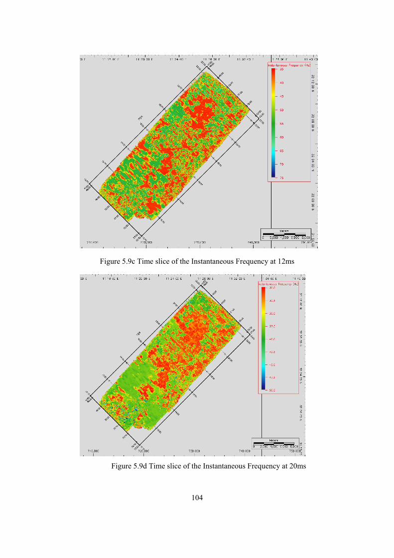
104
Figure 5.9c Time slice of the Instantaneous Frequency at 12ms
Figure 5.9d Time slice of the Instantaneous Frequency at 20ms

105
Figure 5.10a Time slice of the Instantaneous Phase at 2ms
Figure 5.10b Time slice of the Instantaneous Phase at 6ms

106
Figure 5.10c Time slice of the Instantaneous Phase at 10ms
Figure 5.10d Time slice of the Instantaneous Phase at 12ms
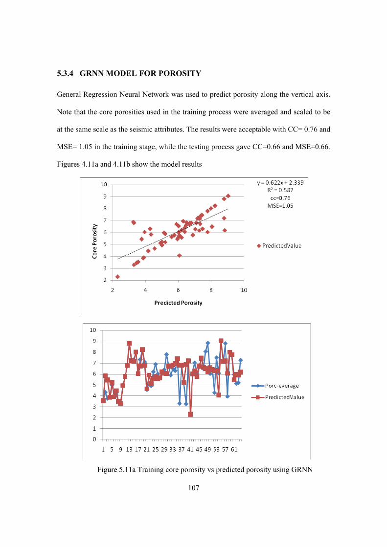
107
5.3.4 GRNN MODEL FOR POROSITY General Regression Neural Network was used to predict porosity along the vertical axis.
Note that the core porosities used in the training process were averaged and scaled to be
at the same scale as the seismic attributes. The results were acceptable with CC= 0.76 and
MSE= 1.05 in the training stage, while the testing process gave CC=0.66 and MSE=0.66.
Figures 4.11a and 4.11b show the model results
Figure 5.11a Training core porosity vs predicted porosity using GRNN

108
Figure 5.11b Testing core porosity vs predicted porosity using GRNN

109
5.3.5 GRNN MODEL FOR PERMEABILITY The same what I did for porosity prediction was also repeated with the permeability model. The results gave CC= 0.83 and MSE = 2.21 in the training process but CC= 0.73 and 0.77 in the testing stage. Figures 4.12a and 4.12b illustrate the model performance.
Figure 5.12a Training core permeability vs predicted permeability using GRNN
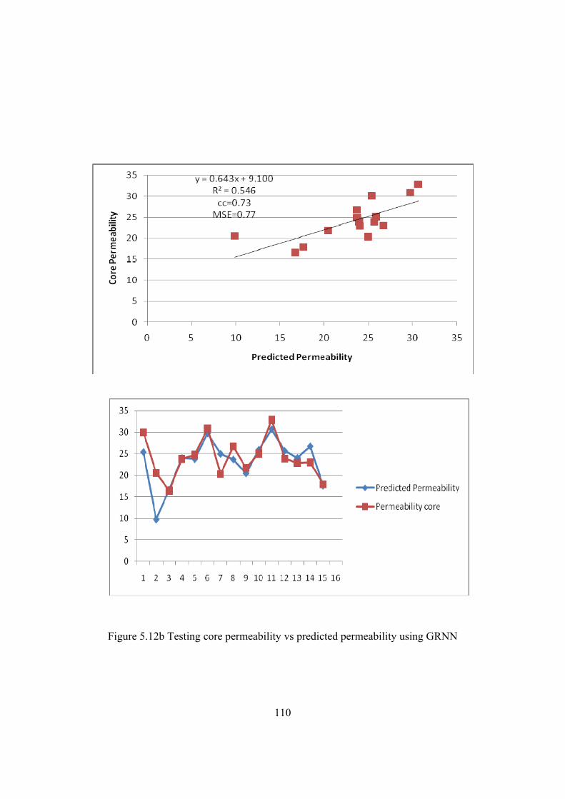
110
Figure 5.12b Testing core permeability vs predicted permeability using GRNN
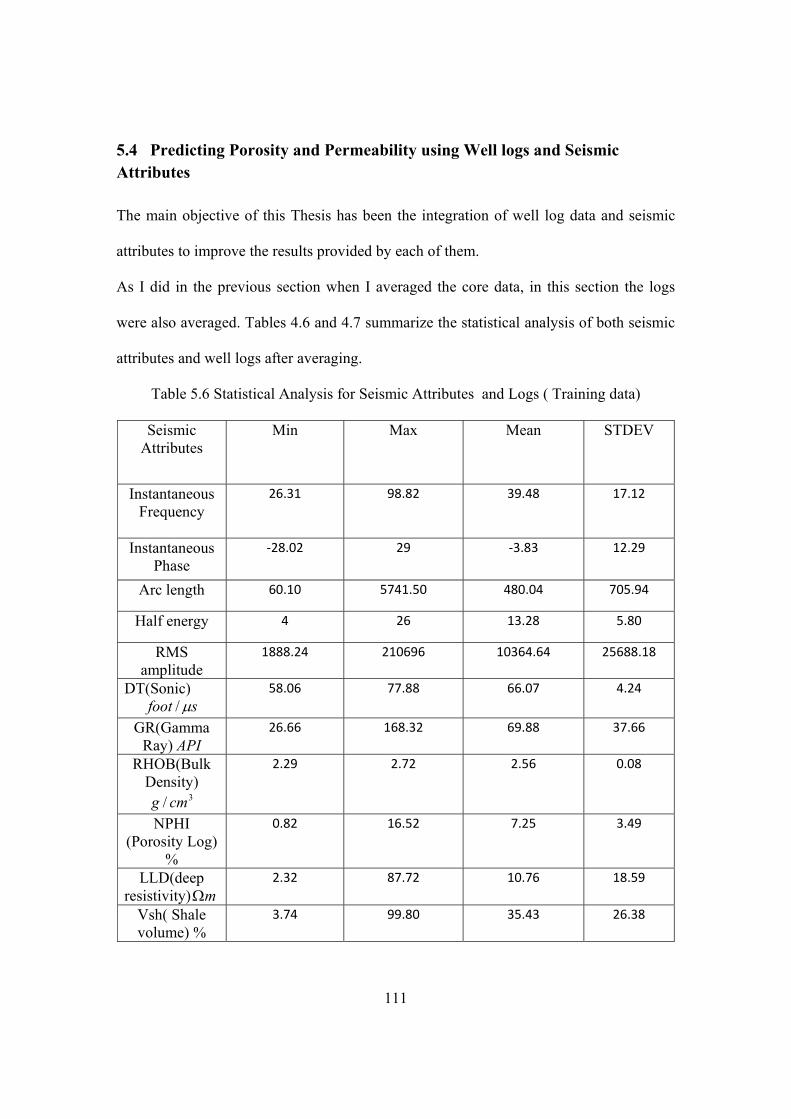
111
5.4 Predicting Porosity and Permeability using Well logs and Seismic Attributes The main objective of this Thesis has been the integration of well log data and seismic
attributes to improve the results provided by each of them.
As I did in the previous section when I averaged the core data, in this section the logs
were also averaged. Tables 4.6 and 4.7 summarize the statistical analysis of both seismic
attributes and well logs after averaging.
Table 5.6 Statistical Analysis for Seismic Attributes and Logs ( Training data)
Seismic Attributes
Min Max Mean STDEV
Instantaneous Frequency
26.31 98.82 39.48 17.12
Instantaneous Phase
‐28.02 29 ‐3.83 12.29
Arc length 60.10 5741.50 480.04 705.94
Half energy 4 26 13.28 5.80
RMS amplitude
1888.24 210696 10364.64 25688.18
DT(Sonic) sfoot μ/
58.06
77.88
66.07
4.24
GR(Gamma Ray) API
26.66
168.32
69.88
37.66
RHOB(Bulk Density)
3/ cmg
2.29
2.72
2.56
0.08
NPHI (Porosity Log)
%
0.82
16.52
7.25
3.49
LLD(deep resistivity) mΩ
2.32
87.72
10.76
18.59
Vsh( Shale volume) %
3.74
99.80
35.43
26.38

112
Table 5.7 Statistical Analysis for Seismic and Logs ( Testing data)
Seismic Attributes and
well logs
Min Max Mean STDEV
Instantaneous Frequency
25.92
40.92
32.65
3.60
Instantaneous Phase
‐43.47
‐0.52
‐21.23
12.18
Arc length 228.8
5741.5 424.9 115.52
Half energy 10
26
18.5
4.98
RMS amplitude
1091.18
7861.8
5834.81
2198.29
DT(Sonic) sfoot μ/
68.44
55.93
62.41
3.74
GR(Gamma Ray) API
102.24
36.73
65.18
20.25
RHOB(Bulk Density)
3/ cmg
2.69
2.20
2.45
0.14
NPHI (Porosity Log)
%
27.86
5.17
11.90
5.94
LLD(deep resistivity) mΩ
102.52
4.47
34.07
35.58
Vsh( Shale volume) %
70.94
4.35
28.42
21.25
5.4.1 GRNN MODEL FOR POROSITY A GRNN model was built to estimate porosity using both seismic attributes and well log
data. The results show CC = 0.93 and MSE =0.29 in the training stage, while testing
produced results with CC= 0.90 and MSE= 0.16. Figures 4.13a and 4.13b show the
model performance
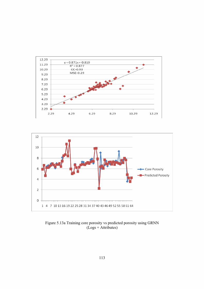
113
Figure 5.13a Training core porosity vs predicted porosity using GRNN (Logs + Attributes)

114
Figure 5.13b Testing core porosity vs predicted porosity using GRNN (Logs + Attributes)

115
5.4.2 GRNN MODEL FOR PERMEABILITY A model was built using GRNN to estimate permeability using both seismic attributes
and well log data. The results show CC = 0.99 and MSE= 0.32 in training stage, while
testing produced results with CC= 0.96 and MSE= 1.29. Figures 4.14a and 4.14b show
the model performance for permeability prediction.
Figure 5.13c Training core permeability vs predicted permeability using GRNN (Logs + Attributes)

116
Figure 5.13d Testing core permeability vs predicted permeability using GRNN (Logs + Attributes)
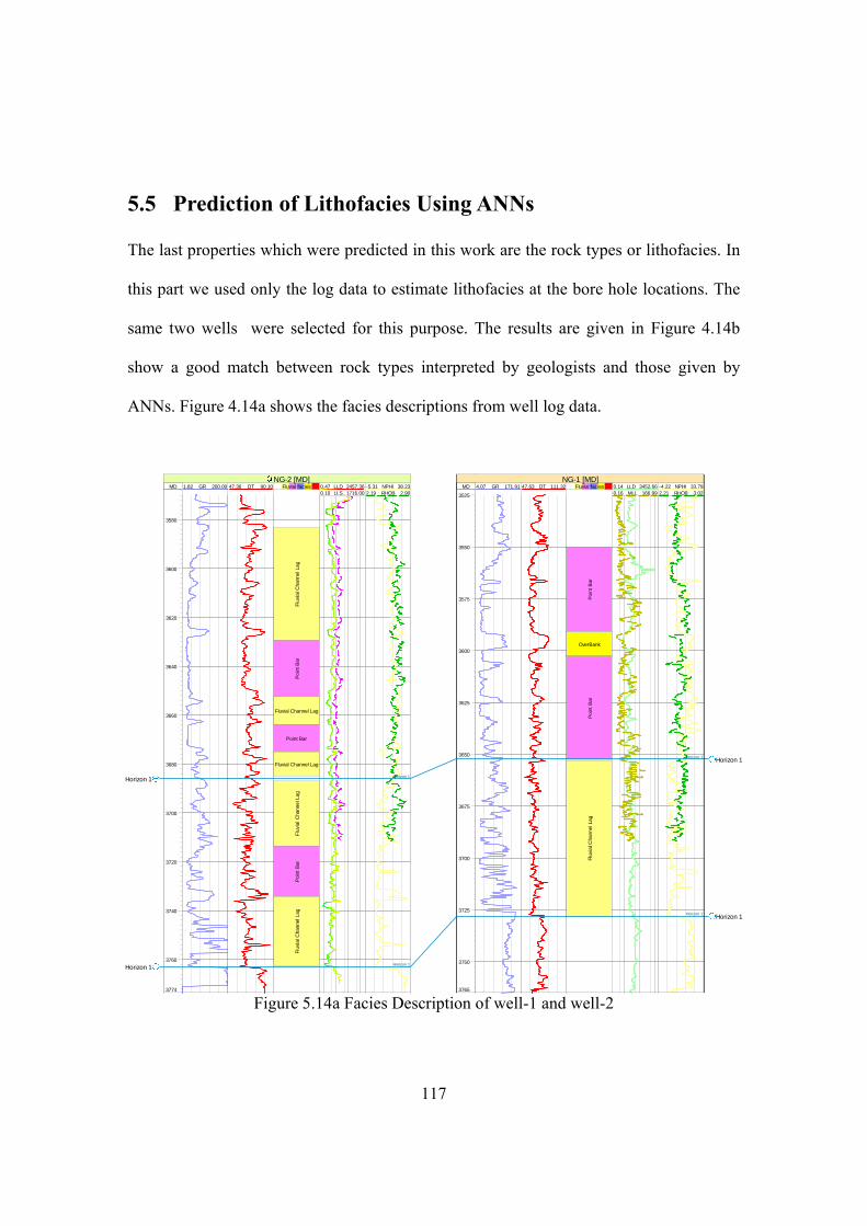
117
5.5 Prediction of Lithofacies Using ANNs The last properties which were predicted in this work are the rock types or lithofacies. In
this part we used only the log data to estimate lithofacies at the bore hole locations. The
same two wells were selected for this purpose. The results are given in Figure 4.14b
show a good match between rock types interpreted by geologists and those given by
ANNs. Figure 4.14a shows the facies descriptions from well log data.
Figure 5.14a Facies Description of well-1 and well-2
Horizon 1
Horizon 1
3580
3600
3620
3640
3660
3680
3700
3720
3740
3760
3774
MD 1.82 200.00GR 47.36 90.10DT
Fluv
ial C
hann
el L
agPo
int B
ar
Fluvial Channel Lag
Point Bar
Fluvial Channel Lag
Fluv
ial C
hann
el L
agPo
int B
arFl
uvia
l Cha
nnel
Lag
Fluvial facies 0.47 2457.36LLD0.10 1716.00LLS
-5.31 38.23NPHI2.19 2.90RHOB
Horizon 1
Horizon 1
NG-2 [MD]
3525
3550
3575
3600
3625
3650
3675
3700
3725
3750
3765
MD 4.07 171.91GR 47.63 111.32DT
Poin
t Bar
OverBank
Poin
t Bar
Fluv
ial C
hann
el L
ag
Fluvial facies 0.14 3452.66LLD0.16 166.99MLL
-4.22 33.79NPHI2.21 3.02RHOB
Horizon 1
Horizon 1
NG-1 [MD]
Horizon 1
Horizon 1
Horizon 1
Horizon 1
3580
3600
3620
3640
3660
3680
3700
3720
3740
3760
3774
MD 1.82 200.00GR 47.36 90.10DT
Fluv
ial C
hann
el L
agPo
int B
ar
Fluvial Channel Lag
Point Bar
Fluvial Channel Lag
Fluv
ial C
hann
el L
agPo
int B
arFl
uvia
l Cha
nnel
Lag
Fluvial facies 0.47 2457.36LLD0.10 1716.00LLS
-5.31 38.23NPHI2.19 2.90RHOB
Horizon 1
Horizon 1
NG-2 [MD]
3525
3550
3575
3600
3625
3650
3675
3700
3725
3750
3765
MD 4.07 171.91GR 47.63 111.32DT
Poin
t Bar
OverBank
Poin
t Bar
Fluv
ial C
hann
el L
ag
Fluvial facies 0.14 3452.66LLD0.16 166.99MLL
-4.22 33.79NPHI2.21 3.02RHOB
Horizon 1
Horizon 1
NG-1 [MD]
Horizon 1
Horizon 1
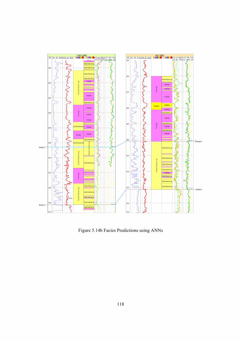
118
Figure 5.14b Facies Predictions using ANNs
Horizon 1
Horizon 1
3580
3600
3620
3640
3660
3680
3700
3720
3740
3760
3774
MD 1.82 200.00GR 47.36 90.10DT
Fluv
ial C
hann
el L
agPo
int B
ar
Fluvial Channel Lag
Point Bar
Fluvial Channel Lag
Fluv
ial C
hann
el L
agPo
int B
arFl
uvia
l Cha
nnel
Lag
Fluvial facies
Point Bar
Fluvial Channel Lag
Fluvial Channel Lag
Fluvial Channel Lag
Fluvial Channel Lag
Point Bar
Point Bar
Fluvial Channel Lag
Point Bar
Point Bar
Point Bar
Point Bar
Point Bar
Fluvial Channel Lag
Fluv
ial C
hann
el L
ag
Fluvial Channel Lag
Fluvial Channel Lag
Fluvial Channel Lag
Fluvial Channel Lag
Fluvial Channel Lag
Fluvial Channel Lag
Fluvial facies [Neural net 1] 0.47 2457.36LLD0.10 1716.00LLS
-5.31 38.23NPHI2.19 2.90RHOB
Horizon 1
Horizon 1
NG-2 [MD]
3525
3550
3575
3600
3625
3650
3675
3700
3725
3750
3765
MD 4.07 171.91GR 47.63 111.32DT
Poin
t Bar
OverBank
Poin
t Bar
Fluv
ial C
hann
el L
ag
Fluvial facies
Fluvial Channel Lag
Point Bar
Point Bar
Point Bar
OverBank
Point Bar
Fluvial Channel Lag
Point Bar
Fluvial Channel Lag
Point Bar
Fluvial Channel Lag
Point Bar
Fluvial Channel Lag
Fluvial Channel Lag
Fluvial Channel Lag
Fluvial Channel Lag
Point Bar
Fluvial Channel Lag
Fluvial Channel Lag
Fluvial Channel Lag
Fluvial facies [Neural net 2] 0.14 3452.66LLD0.16 166.99MLL
-4.22 33.79NPHI2.21 3.02RHOB
Horizon 1
Horizon 1
NG-1 [MD]
Horizon 1
Horizon 1

119
5.6 Predicting the Spatial Distribution of Porosity, Permeability and Lithofaces The last part of this study is to build a 3D model for porosity, permeability and rock type
for a given reservoir. Petrel software from Schlumberger was used to build the 3D grid
from the interpreted seismic surfaces. The model was built using the top and the bottom
of the reservoir. Figure 4.15 shows the seismic interpretation of the three main reservoirs
existing in the study area.
Figure 5.15 Seismic Interpretation of T1, SI and Dev reservoirs in the study area
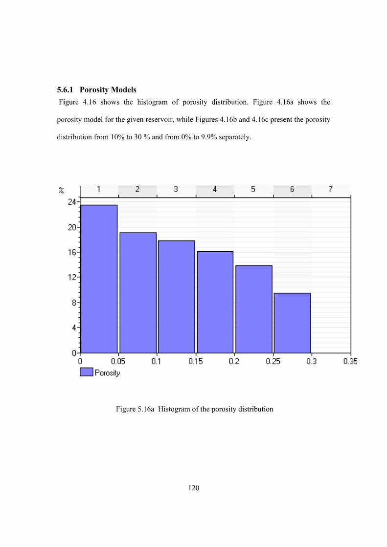
120
5.6.1 Porosity Models Figure 4.16 shows the histogram of porosity distribution. Figure 4.16a shows the
porosity model for the given reservoir, while Figures 4.16b and 4.16c present the porosity
distribution from 10% to 30 % and from 0% to 9.9% separately.
Figure 5.16a Histogram of the porosity distribution

121
Figure 5.16b Porosity distributions in the 3D model for SI Reservoir, pink color indicates low porosity, red color indicates high porosity
Figure.5.16c Porosity (10% - 30 %) distribution in the 3D model for SI Reservoir, pink color indicates low porosity, red color indicates high porosity

122
5.6.2 Permeability Models
Figure 4.17 shows the histogram of permeability distribution. Figure 4.17a illustrates
permeability model obtained using ANNs, while Figure 4.17b shows permeability
distribution from 10 mD to 300mD.
Figure 5.17 Histogram of permeability distribution
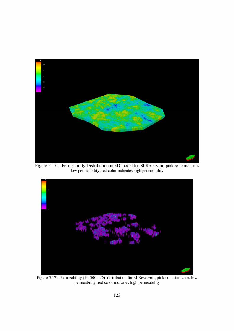
123
Figure 5.17 a. Permeability Distribution in 3D model for SI Reservoir, pink color indicates low permeability, red color indicates high permeability
Figure 5.17b .Permeability (10-300 mD) distribution for SI Reservoir, pink color indicates low permeability, red color indicates high permeability
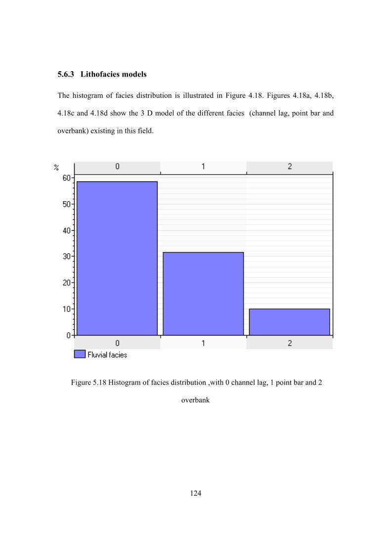
124
5.6.3 Lithofacies models The histogram of facies distribution is illustrated in Figure 4.18. Figures 4.18a, 4.18b,
4.18c and 4.18d show the 3 D model of the different facies (channel lag, point bar and
overbank) existing in this field.
Figure 5.18 Histogram of facies distribution ,with 0 channel lag, 1 point bar and 2
overbank

125
Figure 5.18a Facies model for SI Reservoir , blue color indicates overbank, pink color
point bar and yellow indicates channel lag
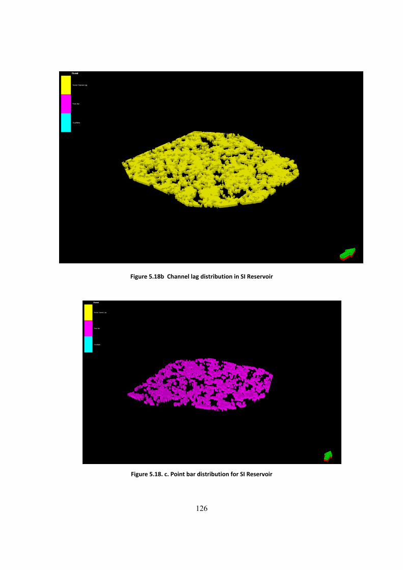
126
Figure 5.18b Channel lag distribution in SI Reservoir
Figure 5.18. c. Point bar distribution for SI Reservoir

127
Figure 5.18d Over bank distribution for SI Reservoir

128
CHAPTER SIX
CONCLUSION AND RECOMMENDATIONS
6.1 Summary
This research work investigated the application of two paradigms in neural networks in
developing accurate models for the prediction of reservoir properties (porosity,
permeability and lithofacies).
The first part of this study focused on designing and investigating multilayer perceptron
(MLP) and general regression neural networks (GRNN) for the prediction of these
reservoir properties using well log data.
From the previous part we selected the best algorithm (GRNN) and we used it to predict
porosity and permeability using seismic attributes derived from 3D seismic volume.
In the third part, we integrated seismic attributes with well log data for better prediction
of reservoir properties.
The last part of this study was to build 3D models for the predicted properties (porosity,
permeability and lithofacies).

129
6.2 Conclusions
Based on the research and analysis discussed previously in this work, the following
conclusions are reached:
• Porosity, permeability and lithofacies can be easily predicted using well log data
rather than coring every well in the field.
• The agreement between the core data and the predicted values by neural networks
demonstrate a successful implementation and validation of the network’s ability
to map complex non-linear relationships between well logs, seismic attributes,
permeability and porosity.
• Results from this study show how powerful general regression neural network
(GRNN) is compared to multilayer perceptron (MLP).
• Multilayer perceptron (MLP) can have good generalization if there is enough time
and knowledge of the network topology.
• The use of seismic attributes combined with well log data gave better prediction
results and enhanced the results reached by using well logs only.
• The 3D geological models gave the full distribution of reservoir properties and
indicated the appropriate zones for future well implementation.
6.3 Recommendations for Future Work
Although good results were obtained from the investigation carried out in this research
work, better accuracy and generalization may be obtained from the following
recommendations:

130
• Investigating using new development of neural network techniques such us
function networks ( FN) and Cascaded correlation neural network (CCNN).
• Using other techniques in artificial intelligence such as support vector machine
( SVM) , fuzzy logic ( FL) and neuro-fuzzy systems ( NFL).
• Investigating combined networks in the form of committee machine or modular
networks where different networks such as Ploynet, FN and GRNN are combined.
These three models were suggested because of the unique results that can be
obtained from them. However, many factors need to be considered in developing
such architecture, including:
1- There are several different methods of combining networks, depending on the
task at hand.
2- Determination of training strategy for different networks to achieve more
accurate network model can be challenging. For example, do we train each
network with the same data set, or different data sets, with overlapping or
without overlapping?
3- Determination of the techniques to combine is also not an easy task.
4- Model complexity versus gained accuracy is another factor to consider.
It is also recommended to integrate more data for more accurate predictions such
as petrography data ( Grain size, Sorting , percentage of cements, gain
shape…ect). It is hoped that implementation of these recommendations will lead
to better models for the prediction of rock properties.
131
References
1) AL-Bazzaz, W. H, Y. W. Al-Mehanna, A. Gupta, Permeability Modeling Using
Neural-Networks Approach for Complex Mauddud-Burgan Carbonate Reservoir
SPE 105337, 2007.
2) Ali .K, Neural Networks: A New Tool for the Petroleum Industry, SPE 1994.
3) Aminzadeh, F. and Brouwer, F. Integrating Neural Networks and Fuzzy Logic for
Improved Reservoir Property Prediction and Prospect Ranking. SEG New Orleans
2006 Annual Meeting.
4) Asquith, G. and Gibson, Ch., Basic Well Log Analysis for Geologists. AAPG
Methods for Exploration Series, Number 3. 1982.
5) Basu Tanwi, Michel Claverie, and David Noland, Kamarolzaman B. Yahya and
Mustafa Suleiman, Facies Analysis: Integration of Core and Log Data using a
Neural Networks as Input for Reservoir Modeling in Betty Field, Malaysia. The
Leading Edge, v. 23; no. 8; pp. 794-797, 2004.
6) Baldwin, J. L. , Bateman, A. R. M. , Wheatley, C. L. , 1990. Application of Neural
Network to the Problem of Mineral Identification from Well Logs. The Log
Analyst 3, pp. 279–293.
7) Balan, B. , Mohaghegh, S. , Ameri, S. , 1995. State-of-the-Art in Permeability
Determination from Well Log Data: Part I. Comparative study, model
development. SPE Eastern Regional Conference and Exhibition, West Virginia,
pp. 17–21.
8) Bean M. and Jutten C., 2000. Neural Networks in Geophysical Applications.
Geophysics, 65, pp. 1032-1047.
132
9) Bel F. and Demargne F,1996. Etude Géologique du Terminal ANRH, Alger,
Algérie, pp. 22.
10) Bellaoueur. A, 2008. Etude hydrogéologique des eaux souterraines de la région de
Ouargla soumise a la remontée des eaux de la nappe phréatique et perspectives de
solutions palliatives. Mémoire de Magister, L’université El-Hadj lakhdar, Batna,
Algerie.
11) Bhatt A. and Helle H. B, 2002. Committee Neural Networks for Porosity and
Permeability Prediction from Well Logs. Geophysical Prospecting, 50, pp. 645-
660.
12) Black, M.: Reasoning with Loose Concepts. Dialogue (2) 1–12 (1963).
13) Brown, A.R., 1996, Seismic attributes and their classification. The Leading Edge,
15, p.1090.
14) Brown, A. R., 2001, Understanding seismic attributes: Geophysics, 66, pp. 47-48.
15) Busson.G, 1970. Principes, Méthodes et Résultats d’une étude stratigraphique du
Mésozoïque saharien. Mémoire Muséum Histoire Naturelle Paris, série C XXVI
(1972), p. 441.
16) Chang H.C., Kopaska-Merkel D. C., Chen H.C. and Durrans S. R., Lithofacies
Identification using Multiple Adaptive Resonance Theory Neural Networks and
Group Decision Expert System, Computers and Geosciences, 26, Number 5, 1
June 2000, pp. 591-601.
17) Chen, Q. and Sidney, S.,1997, Seismic attribute technology for reservoir
forecasting and monitoring. The Leading Edge, 16, No.5, pp. 445-450.

133
18) Cheng Dang Zou, Xi-Ling Wu, and Ju-An Cheng, Determination of Reservoir
Properties using a Fuzzy Neural Network, SPE 26430, 68th Annual Technical
Conference and Exhibition, Houston, Texas, 3-6 October 1993.
19) Christian Perrin, Mohamed Rafik, Mahmoud Akbar, Samir Jain, Integration of
Borehole Image to Enhance Conventional Electrofacies Analysis in Dual Porosity
Carbonate Reservoirs, SPE 11622, International Petroleum Technology
Conference, Dubai, UAE 4-6 December 2007.
20) Daniel J. Leiphart and Bruce S. Hart, Case History Comparison of Linear
Regression and Probabilistic Neural Network to Predict Porosity from 3-D seismic
Attributes in Lower Brushy Canyon Channel Sandstones, Southeast New Mexico,
Geophysics, Vol.66, No. 5, 2001, pp. 1349-1358.
21) Djabbar Tiab and Erle. C. Donaldson, Petrophysics. Theory and Practice of
Measuring Reservoir Rock and Fluid Transport Properties. 1996 Gulf Publishing
Company, Houston, Texas.
22) Doyen, P. M., 1998, Porosity from seismic data -A geostatistical approach:
Geophysics, 3, pp. 1263-1275.
23) Dubief, J., 1963. Le climat du Sahara. Memoire Institut des Recherches
Sahariennes. Tome 1 & 2, Alger, 317 + 275 pp.
24) Eshafei, M. and Gharib, M., Neural Network Identification of Hydrocarbon
Potential of Shaly Sand Reservoirs , Technical Symposium SPE, 2007 .
25) Fabre, J, 1976. Introduction à la Géologie du Sahara algérien. SNED, Alger,
Algerie, 422 pp.

134
26) Fruhwirth R.K., Thonhauser, G. and W. Mathis, Hybrid Simulation using Neural
Networks to Predict Drilling Hydraulics in Real Time. SPE Paper 103217, SPE
Annual Technical Conference and Exhibition, San Antonio, Texas, U.S.A., 24–27
September 2006.
27) Garrouch, N. and Smaoui, H., An Artificial Neural Network Model for Estimating
Tight gacs sand Permeability, SPE 39703, 1994.
28) Geology of Algeria, Sonatrach Exploration Division, Research and Development
Centre and Petroleum Engineering and Development Division. pp 93.
29) Guangyi Hu, Xuri Huang, Mingxiang Mei, Li Gu and Chaozheng Xiao,
Characterization of a Reef Reservoir Permeability using Well and Seismic Data,
SPE 110179, SPE Annual Technical Conference and Exhibition, California, USA,
11-14 November, 2007.
30) Jeff Heaton, Introduction to Neural Networks with Java. Heaton Research, Inc.,
2005.
31) Hampson, D.P., Schuelke, J.S., and Quirein, J.A., 2001, Use of multiattribute
transforms to predict log properties from seismic data: Geophysics, v. 66, pp. 220-
236.
32) Herrera, V.M., Russell, B., and Flores, A., Neural Networks in Reservoir
Characterization, The Leading Edge, 25, no. 4 (2006): pp. 402-411.
33) Lianshuang Qi, Timothy R. Carr, Neural Network Prediction of Carbonate
Lithofacies from Well Logs, Big Bow and Sand Arroyo Creek Fields, Southwest
Kansas, Computers and Geosciences 32 (2006) pp. 947–964.
34) Lucia, F.J., Carbonate Reservoir Characterization. Springer, 1999 .
135
35) Mari, J.-L, GlanGeaud, F and Coppens F., Signal Processing for Geologists and
Geophysicists . Édition Technip, Paris, 1997.
36) Masters, T., Practical Neural Networks Recipes in C++ , Elsevier, 1993.
37) Matos, M.C., Osório, P.L.M. and Johann, P.R.S., Unsupervised Seismic Facies
Analysis Using Wavelet Transform and Self Organization Maps, Geophysics, Vol.
72, No. 1 (2007); pp. 9-21.
38) Mial, A.D., The Geology of Fluvial Deposits: Sedimentary Facies, Basin Analysis
and Petroleum Geology: Springer-Verlag, Berlin, 582 pp., 1996.
39) Mohaghegh S., Arefi R., Ameri S. and Rose D., Design and Development of an
Artificial Neural Network for Estimation of Permeability, SPE 28237, SPE Petr.
Computer Conference, Dallas, Texas, USA, July 31 – August 3, 1994.
40) Moline, G.R. and Bahr, J.M., Estimating spatial distributions of heterogeneous
subsurface characteristics by regionalized classification of electrofacies.
Mathematical Geology 27, pp. 3–22, 1995.
41) Osborne, D. A. Neural Networks Provide More Accurate Reservoir Permeability.
Oil and Gas Journal , Sept., 1992, pp. 80-83.
42) Oss (2003a et b), Système aquifère du Sahara septentrional. Rapport interne.
Annexes, Tunis, Tunisie, pp229.
43) Ouja M, 2003. Etude sedimentologique et paléobotanique du jurassique moyen-
crétacé inferieur du basin de Tataouine. Phd, Université Claude Bernard. Lyon,
pp164.
44) Raiche, A., A Pattern Recognition Approach to Geophysical Inversion using
Neural Nets. Geophysical Journal International 105, pp. 629–648, 1991.
136
45) Rivera Vega Nestor, Reservoir Characterization using Wavelet Transforms. Texas
A and M University Thesis, 2003.
46) Rogers, S.J., Fang, J.H., Karr, C.L. and Stanley, D.A., Determination of lithology
from well logs using a neural network. American Association of Petroleum
Geologists Bulletin 76 (1992): pp. 731–739.
47) Russell, B., Vagueness. Austrian Journal of Philosophy (1) (1923) pp. 84-92.
48) Salan B., Mohaghegh S. and Ameri S., Permeability Determination from Well Log
Data: A Comparative Study, Model Development. SPE 30978, 1995.
49) Saggaf, M.M., Toksöz, M.N. and Marhoon, M.I., Seismic Facies Classification
and Identification by Competitive Neural Networks, Geophysics ,Vol. 68, No. 6
(November-December 2003); pp. 1984-1999.
50) Schutz, P.S Hattori, M and Corbett, C., 1994, Seismic guided estimation of log
properties, parts 1,2, and 3: The Leading Edge,13,305-310,674-678, and 770-776.
51) Sheriff, R.E., 1992, Reservoir Geophysics, IG No.7, Edited By SEG, 408pp.
52) Sippel, M., Reservoir Characterization from Seismic and Well Control with
Intelligent Computing Software, AAPG Annual Convention, Salt Lake City, Utah,
May 11-14, 2003.
53) Soto, R.B., Bernal, M.C. and Silva, B., How to Improve Reservoir
Characterization using Intelligent Systems. SPE 62938, 2000.
54) Soto, R., Torres, B.F., Arango, S. and Cobaleda, G., Improved Reservoir
Permeability Models from Flow Units and Soft Computing Techniques. A Case
Study, Suria and Reforma-Libertad, SPE 69625, 2001.

137
55) Taner, M.T., Koehler, F., and Sheriff, R.F., 1979, Complex seismic trace analysis.
Geophysics, 44,1041-1063.
56) Taner, M.T., Schuelke, J.S., O’Doherty, R., Baysal, E., 1994, Seismic attributes
revisited: 64th Annual Internal Mtg, SEG., Expanded Abstracts, 1104-1106.
57) Tamhane, P., Wong, M., and Aminzadeh, F., Soft Computing for Intelligent
Reservoir Characterization, SPE 59397, 2000.
58) Trappe H and Hellmich C., 1998, Seismic characterization of Rotliegend reservoir;
from bright spots to stochastic simulation: First Break, 16, pp. 79-87.
59) Van der Baan, M. and Jutten, Ch., Neural Networks in Geophysical Applications.
Geophysics, Vol. 65, No. 4 (2000); pp. 1032-1047.

138
VITAE
Mohamed Sitouah was born on September 02,1978 in Bordj Menail Algeria. He
graduated from Boumerdes University in 2002 with bachelor degree in Geophysics.
He then joined the Algerian Company of Geophysics ( ENAGEO) as Geophysicist and
worked there till January 2007. Mohamed Sitouah joined earth Sciences Department at
King Fahd University of Petroleum & Minerals in February 2007, as a Research assistant
and completed his Master of Science ( MSc ) majoring in Geophysics in June 2009.
His areas of research include:
1- Seismic acquisition & Quality Control.
2- Seismic Data Processing ( Promax, SU).
3- Reservoir Characterization
4- Reservoir Geophysics
5- Reservoir Monitoring (4 D Seismic )
6- Well Logging Interpretation
7- Geostatistical Modeling
8- Geological Modeling