estimation of optimal crop plan using nature inspired ... of optimal crop plan using nature inspired...

ISSN 1 746-7233, England, UKWorld Journal of Modelling and Simulation

Vol. 6 (2010) No. 2, pp. 97-109

Estimation of optimal crop plan using nature inspired metaheuristics

Millie Pant1, Radha Thangaraj1∗, Deepti Rani2, Ajith Abraham3, Dinesh Kumar Srivastava4

1 Department of Paper Technology, Indian Institute of Technology Roorkee, Saharanpur 247 001, India2 Department of Rural Engineering, University of Evora, Evora 7002-054, Portugal

3 Center of Excellence for Quantifiable Quality of Service, Norwegian University of Science and Technology, TrondhiemNO-7491, Norway

4 Department of Hydrology, Indian Institute of Technology Roorkee, Roorkee 247 667, India

(Received December 15 2008, Revised October 11 2009, Accepted October 23 2009)

Abstract. Irrigation management has gained significance due to growing social needs and increasing com-mand for food grains while the available resources have remained limited and scarce. Irrigation managementincludes optimal allocation of water for irrigation purposes, optimal cropping pattern for a given land areaand water availabilities with an objective to maximize economic returns. In the present study we consideran optimization model based on linear programming for determining optimal crop plan for command areaof Pamba-Achankovil-Vaippar (PAV) link project, Kerala, India. The crop planning model considers variousresource constraints (land area, seeds, manure, fertilizers etc.) availability etc. adaptive to national conditions,with the objective to maximize net irrigation benefits. For crop planning, the extent of quantity available forfertilizers, manure and seeds as inputs were unknown. Estimates for the extent of unknown minimum quan-tities of these resource inputs available are obtained with the help of crop planning model itself. For optimalreleases made from reservoir using a multi-reservoir operation model, optimal crop plans are developed underadequate, normal and limited irrigation water defined by 50 percent, 75 percent and 90 percent water year de-pendable flows, respectively. The optimization model is solved using four popular Evolutionary Algorithms(EA) viz. Genetic Algorithms (GA), Particle Swarm Optimization (PSO), Differential Evolution (DE) andEvolutionary Programming (EP). EA are compared with each other in terms of average CPU time, averagenumber of generations, standard deviation etc. the algorithms are also compared with LINGO, a popularsoftware used for solving LPP models.

Keywords: evolutionary algorithms, reservoir, crop plan, constrained optimization, penalty function

1 Introduction

Agriculture in India is one of the most prominent sectors in its economy. Agriculture and allied sectorslike forestry, logging and fishing accounts nearly for 16.6% of the GDP and 8.56% of India’s exports. About43% of India’s geographical area is used for agricultural activity. About 70% of India is directly dependenton agriculture, which is the main component of most state economies in India. The dependence of agricultureon monsoon has boosted the need of irrigation management. Also, it is worth mentioning that most of theirrigation management problems can be formulated as optimization models. Some of the interesting examplesinclude Windsor and Chow[30], who developed a multilevel optimization model for a farm irrigation system.Linear programming (LP) was used by them at second level of optimization for optimal land and water al-location. At first level dynamic programming was used to estimate the expected data for LP model. Rogersand Smith[22] employed the interaction of surface and ground water systems in irrigation management usingdeterministic LP model.

∗ Corresponding author. Tel.: +91-9808517165, fax: +91-132-2714311; E-mail address: [email protected].

Published by World Academic Press, World Academic Union

98 M. Pant & R. Thangaraj & et al.: Estimation of optimal crop plan

Lakshminarayan and Raja Gopalan[16] used an LP model to determine an optimal cropping patternand optimal release policy from canals and tube wells for maximizing the economic returns. Matanga andMarinno[19] and Chavez-Morales et al.[4] used linear optimization models to obtain optimal cropping patternswith different objective functions. Two chance constrained LP models were formulated by Maji and Heady[18]

to maximize net return from project area for the Mayurakshi project in India. Raju and Kumar[12] proposed acrop planning model with the objective of maximizing irrigation benefits for a typical irrigation system. Kuoet al.[15] used Genetic Algorithm (GA) based model for irrigation project planning for case study of Delta,Utah with the objective of maximization of net economic benefits for a cultivable command area of 394.6 ha.Raju and Kumar[25] applied Genetic Algorithms for irrigation planning in Indian context and compared theresults with LP approach. Their results showed the comparable performance of GA with LP. In an applicationoriented research article, Mayer et al.[20] discussed the optimal parameter settings of Evolutionary Algorithmsfor optimization of agricultural system models. In one of the recent studies Zhang et al.[31] studied the cornoptimization irrigation model using Genetic Algorithms.

For the present study we analyzed the performance of four EA namely GA, EP, PSO and DE to obtainoptimal crop plans under adequate, normal and limited irrigation water availability for irrigation area subjectto various constraints in context of the national scenario, under the PAV link project, India. Penalty functionmethod is used for dealing with constraints while using EA.

2 Study area: Pamba-Achankovil-Vaippar Link project, Kerala, India submitting

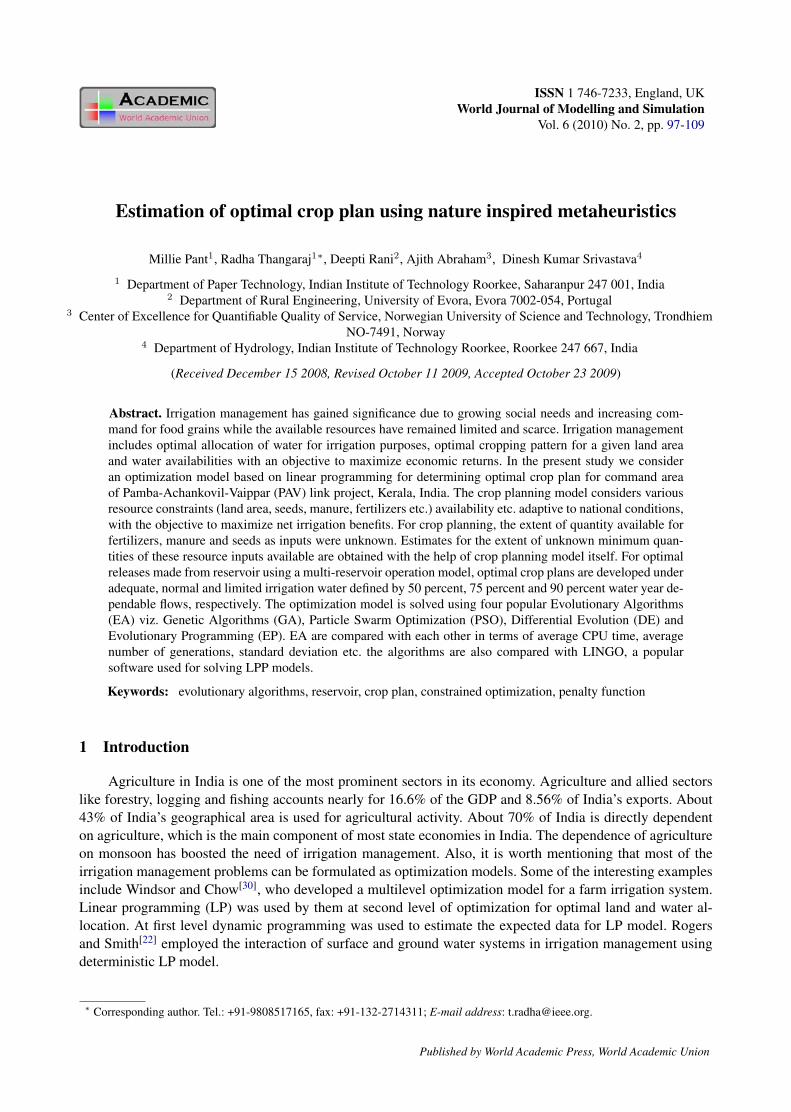
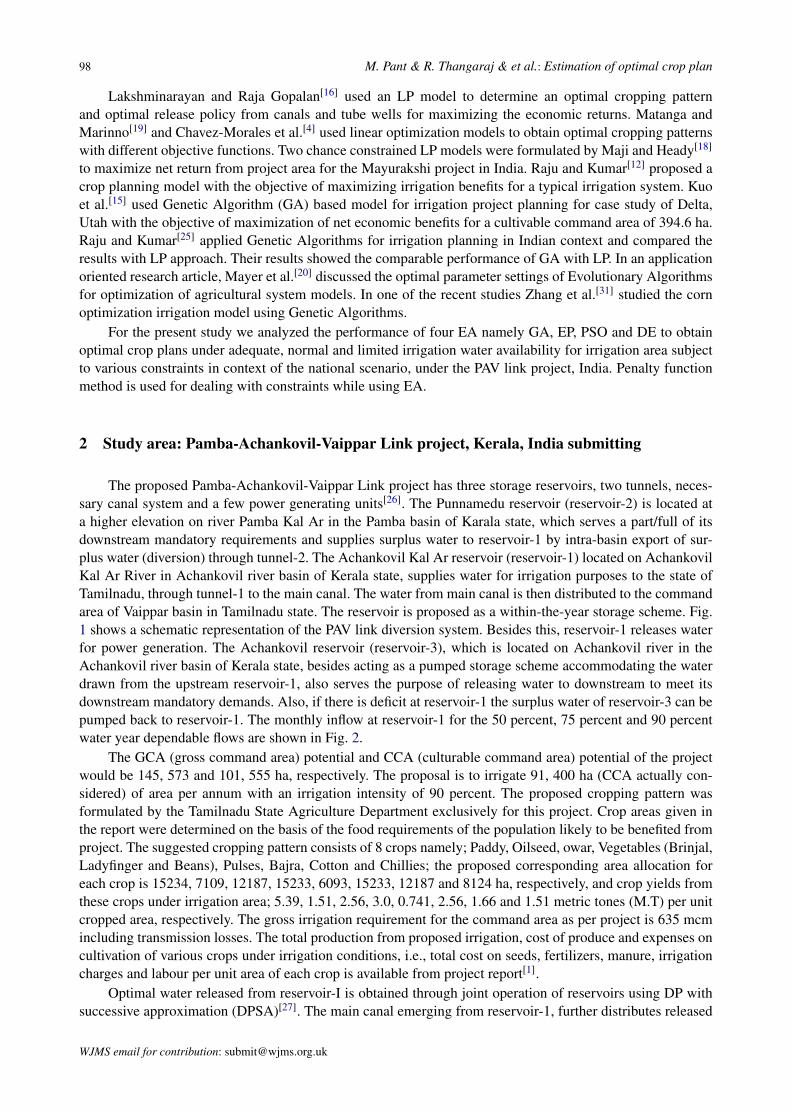
The proposed Pamba-Achankovil-Vaippar Link project has three storage reservoirs, two tunnels, neces-sary canal system and a few power generating units[26]. The Punnamedu reservoir (reservoir-2) is located ata higher elevation on river Pamba Kal Ar in the Pamba basin of Karala state, which serves a part/full of itsdownstream mandatory requirements and supplies surplus water to reservoir-1 by intra-basin export of sur-plus water (diversion) through tunnel-2. The Achankovil Kal Ar reservoir (reservoir-1) located on AchankovilKal Ar River in Achankovil river basin of Kerala state, supplies water for irrigation purposes to the state ofTamilnadu, through tunnel-1 to the main canal. The water from main canal is then distributed to the commandarea of Vaippar basin in Tamilnadu state. The reservoir is proposed as a within-the-year storage scheme. Fig.1 shows a schematic representation of the PAV link diversion system. Besides this, reservoir-1 releases waterfor power generation. The Achankovil reservoir (reservoir-3), which is located on Achankovil river in theAchankovil river basin of Kerala state, besides acting as a pumped storage scheme accommodating the waterdrawn from the upstream reservoir-1, also serves the purpose of releasing water to downstream to meet itsdownstream mandatory demands. Also, if there is deficit at reservoir-1 the surplus water of reservoir-3 can bepumped back to reservoir-1. The monthly inflow at reservoir-1 for the 50 percent, 75 percent and 90 percentwater year dependable flows are shown in Fig. 2.

The GCA (gross command area) potential and CCA (culturable command area) potential of the projectwould be 145, 573 and 101, 555 ha, respectively. The proposal is to irrigate 91, 400 ha (CCA actually con-sidered) of area per annum with an irrigation intensity of 90 percent. The proposed cropping pattern wasformulated by the Tamilnadu State Agriculture Department exclusively for this project. Crop areas given inthe report were determined on the basis of the food requirements of the population likely to be benefited fromproject. The suggested cropping pattern consists of 8 crops namely; Paddy, Oilseed, owar, Vegetables (Brinjal,Ladyfinger and Beans), Pulses, Bajra, Cotton and Chillies; the proposed corresponding area allocation foreach crop is 15234, 7109, 12187, 15233, 6093, 15233, 12187 and 8124 ha, respectively, and crop yields fromthese crops under irrigation area; 5.39, 1.51, 2.56, 3.0, 0.741, 2.56, 1.66 and 1.51 metric tones (M.T) per unitcropped area, respectively. The gross irrigation requirement for the command area as per project is 635 mcmincluding transmission losses. The total production from proposed irrigation, cost of produce and expenses oncultivation of various crops under irrigation conditions, i.e., total cost on seeds, fertilizers, manure, irrigationcharges and labour per unit area of each crop is available from project report[1].

Optimal water released from reservoir-I is obtained through joint operation of reservoirs using DP withsuccessive approximation (DPSA)[27]. The main canal emerging from reservoir-1, further distributes released

WJMS email for contribution: [email protected]

World Journal of Modelling and Simulation, Vol. 6 (2010) No. 2, pp. 97-109 99

water to users (Reach-I, II and III). In this study optimal cropping pattern is obtained for the total area lyingunder Reach-I, II and III.

Fig. 1. Schematic diagram for PAV link diversion system

Fig. 2. Monthly inflows at Reservoir-I

3 Evolutionary algorithms used for comparison

Evolutionary Algorithms (EAs) may be termed as general purpose algorithms for solving optimizationproblems. These algorithms have been successfully applied to a wide range of problems occurring in variousfields[17, 23, 24]. Each EA is assisted with special operators that are based on some natural phenomenon. Thesealgorithms are iterative in nature and in each iteration special operators are invoked to manipulate the popu-lation of candidate solutions in order to reach to optimal (or near optimal) solution. Although all algorithmshave same modus-operendi like starting with a population of candidate solutions which are manipulated so asto be guided towards the optimum solution, each algorithm has certain unique feature associated with it whichmakes it different. A brief description of the three EAs used in this study is given in the following subsections.Pseudo codes of the algorithms used in the present study are given in Appendix.

3.1 Genetic algorithms

Genetic Algorithms (GAs) are perhaps the most commonly used EA for solving optimization problems.In fact it was the success of GAs that made the concept of EAs widely popular for solving various optimizationproblems. The natural phenomenon which forms the basis of GA is the concept of survival of the fittest. GAswere first suggested by John Holland[11]. The main operators of GA are Selection, Reproduction and Mutation.GAs work with a population of solutions called chromosomes. The fitness of each chromosome is determined

WJMS email for subscription: [email protected]


by evaluating it against an objective function. The chromosomes then exchange information through crossoveror mutation. In the present study we have used arithmetic crossover[21]. It is a two parent crossover operationin which two individuals selected from the population undergo reproduction to produce two new offspring.The working of Arithmetic Crossover may be defined as: Arithmetic Crossover: if Pi and Pj are two parentsthe offsprings Ci and Cj are generated as: Ci = a× Pi + (1− a)× Pj ;Cj = (1− a)× Pi + a× Pj . Where‘a’ may be taken as a constant or variable. The Arithmetic Crossover is followed by Gaussian mutation wherea Gaussian noise is added to the particles to add perturbation to the particles. More detail on the working ofGAs may be obtained from [5, 10, 21] etc.

3.2 Particle swarm optimization

Particle swarm optimization (PSO) was first suggested by Kennedy and Eberhart[14]. The mechanism ofPSO is inspired from the complex social behavior shown by the natural species. For a D-dimensional searchspace the position of the ith particle is represented as Xi = (xi1, xi2, · · · , xiD). Each particle maintains amemory of its previous best position Pi = (pi1, pi2, · · · , piD) and a velocity Vi = (vi1, vi2, · · · , viD) alongeach dimension. At each iteration, the P vector of the particle with best fitness in the local neighborhood,designated g, and the P vector of the current particle are combined to adjust the velocity along each dimensionand a new position of the particle is determined using that velocity. The two basic equations which govern theworking of PSO are that of velocity vector and position vector are given by:

vid = ωvid + c1r1(pid − xid) + c2r2(pgd − xid); (1)

xid = xid + vid. (2)

The first part of Eq. (1) represents the inertia of the previous velocity, the second part is tells us about thepersonal thinking of the particle and the third part represents the cooperation among particles and is thereforenamed as the social component. Acceleration constants c1, c2 and inertia weight are predefined by the userand r1, r2 are the uniformly generated random numbers in the range of [0, 1].

3.3 Differential evolution

Differential Evolution was proposed by Storn and Price[28]. It is a population based algorithm like geneticalgorithms using the similar operators; crossover, mutation and selection. The main difference in constructingbetter solutions is that genetic algorithms rely on crossover while DE relies on mutation operator[13]. DE worksas follows: First, all individuals are initialized with uniformly distributed random numbers and evaluated usingthe fitness function provided. Then the following will be executed until maximum number of generation hasbeen reached or an optimum solution is found.

For a D-dimensional search space, each target vector xi,g, a mutant vector is generated by:

vi,g+1 = xr1,g + F × (xr2,g − xr3,g), (3)

where r1, r2, r3 ∈ {1, 2, · · · , NP} are randomly chosen integers, must be different from each other and alsodifferent from the running index i. F (x > 0) is a scaling factor which controls the amplification of the differ-ential evolution xr2,g − xr3,g. In order to increase the diversity of the perturbed parameter vectors, crossoveris introduced[29]. The parent vector is mixed with the mutated vector to produce a trial vector uj,i,g+1,

uj,i,g+1 ={vj,i,g+1 if randj ≤ Cr

∨j = k

xj,i,g otherwise(4)

where j = 1, 2, · · · , D; randj ∈ [0, 1]; CR is the crossover constant takes values in the range [0, 1] andjrand ∈ (1, 2, · · · , D) is the randomly chosen index.

Selection is the step to choose the vector between the target vector and the trial vector with the aim ofcreating an individual for the next generation. Several versions of DE are available in literature. In the presentstudy we use the DE/rand/1/bin-version, which is apparently the most commonly used version.



3.4 Evolutionary programming

Initially, Evolutionary Programming (EP) was introduced as an evolutionary approach to artificialintelligence[9], however, it has been successfully applied to many numerical optimization problems[6–8]. Opti-mization by EP consists of two major steps:

• Mutate all the solutions in the current population.

• Select the next generation from the mutated and the current solutions.

In the present article we use self adaptive EP (SAEP) which was introduced by Back and Schwefel[3] andFogel[8] and was shown to be more efficient than the normal EP. In SAEP each individual is taken as a pair ofreal-valued vectors, (xi, σi) for all i = 1, · · · ,M . The xi’s give the ith member’s object variables and σi’s theassociated strategy parameters. The objective function is evaluated for each individual. Mutation in EP createsa single offspring (x

′i, σ

′i) for all i = 1, · · · ,M by

σ′i(j) = σi(j) exp(τN(0, 1) + τ

′Nj(0, 1));

x′i(j) = xi(j) + σ

′i(j)Nj(0, 1) for all j = 1, · · · , n. (5)

WhereN(0, 1) denotes a random number distributed by Gaussian or Cauchy distribution. In the present articlewe used Cauchy mutation. The factors τ and τ

′are commonly set to 1/

√2n and 1/

√2√n respectively.

3.5 Penalty method for solving constrained optimization problems

The mathematical model considered in the present study is subject to various constraints and penaltyfunction approach is used to solve the constraints. The search space in Constrained Optimization Problems(COPs) consists of two kinds of solutions: feasible and infeasible. Feasible points satisfy all the constraints,while infeasible points violate at least one of them. Therefore the final solution of an optimization problemmust satisfy all constraints. In the penalty function approach, the constrained problem is transformed into anunconstrained optimization algorithm by penalizing the constraints and building a single objective function,which is minimized using an unconstrained optimization algorithm. That is,

F (x) = f(x) + λp(x), (6)

where

p(xi, t) =ng+nh∑m=1

λm(t)pm(xi); (7)

pm(xi) = max{0, gm(xi)α} ifm ∈ [1, · · · , ng] (intequality); (8)

pm(xi) = |hm(xi)|α ifm ∈ [ng + 1, · · · , ng + nh] (equality). (9)

Where α is a positive constant representing the power of the penalty. The inequality constraints are consideredas g(x) and h(x) represents the equality constraints. ng and nh denotes the number inequality and equalityconstraints respectively. λ is the constraint penalty coefficient.

4 Mathematical model

A linear programming based optimization model is used for crop planning. The model maximizes netreturns from crops and yields optimal crop plan and monthly releases required from reservoir-1. Surface water,land availability, fertilizers (N , P , and K), seeds and manure requirements are considered as constraints inthe model. For the purpose of modeling, the crops have been segregated as food grains, cash crops and others.Paddy, Jowar and Bajra are clubbed together as these falls under the category of food grains.



Crop planning model

maxZ = GT − PT . (10)

Where

GT =N∑

i=1

yibiAi and PT =N∑

i=1

(CSi + CMi + CFi + CIi + CLHi)Ai.

Subject to:

N∑i=1

(Wi,t)Ai ≤ Rt for all t (11)

N∑i=1

(λi,t)Ai ≤ AT andN∑

i=1

Ai ≤ AT (12)∑i

yiAi ≥∑

i

yiT for i = 1, 3 and 6 and yiAi ≥ yi

T (13)

N∑i=1

Ff,iAi ≤ Ff,T for all f (14)

N∑i=1

MiAi ≤MT (15)

SiAi ≤ ST for all i (16)

Ai,min ≤ Ai ≤ Ai,max (17)

In the above model, Eq. (10) represents the objective function to maximize the net returns from crops andyields optimal crop plan. Eqs. (11) ∼ (17) represent constraints. Surface water availability constraints whichshould be less than or equal to the surface water available is given by Eq. (11) and land availability constraintswhich should be less than or equal to the total area available are given by Eq. (12). Eq. (13) represents the yieldrequirement constraint which should be greater than or equal to the proposed yield requirement. Fertilizersavailability constraints are given by Eq. (14). Three types of fertilizers have been considered in the applicationof model, i.e., Nitrogen, Phosphorus and Potassium (N , P , K). Manure and Seed Availability Constraintsare given by (15) and (16) respectively. Constraint (9) gives the Seeds Availability Constraints and finally theBounds on Areas under Various Crops are given by Eq. (17). Index i = 1, 2, · · · , 8 represents various cropsfor Paddy, Oilseeds, Jowar, Vegetables, Pulses, Bajra, Cotton and Chilies respectively.

A minimum crop area constraint has been specified on each crop so as to see that area occupied bycrops does not fall below area under rain-fed cultivation. It has also been specified that area proposed undercotton and chilies should not be more than 18 percent and 17 percent of annual irrigation. This condition isjustified because their yields have high revenues and optimally higher area allocation to these crops may causereduction in food grain output, which is socially undesirable. It has been considered essential that total foodgrain production should not be less than 101, 995 M.T.

5 Experimental settings

In this section we give the data used for the mathematical model used in section 3 and the parametersettings for EA. From information available[2] estimates of average values of quantities/ha required for eachcrop for resource inputs, i.e., seeds, manure and fertilizers are obtained. Total requirements of these resourcesare obtained from these values and crop area allocation as per project report. Initially it was assumed that total



quantity available for each resource is equal to total quantity required for the resource. The crop planningmodel is solved using LINGO package. The first trial run is made of the model assuming that the amount ofeach resource available is equal to the required amount, and from results it was seen that out of the total CCA,i.e., 91400 ha only 88818.64 ha is allocated to the crops, i.e., with this trial the total CCA was not allocatedto various crops (please also see Tab. 1). Further model runs were made by varying quantity of resourceavailability in some percent of required amount the area allocations for these trials are given in Tab. 1.

Table 1. Optimal area allocations with variable resource inputs available

Resource Inputs Optimal Area Allocations (ha)80% 73120.0090% 74384.31

100% 88818.64110% 89754.08130% 91400.00

Table 2. Extents of resource available

ResourceExtent

Availability+

Fertilizers(kg)N 5774510P 4911240K 2303256

Manure (M.T.) 1431135

Seeds(kg)

Paddy 1188252Oil seeds 2102154

Jowar 93838.8Vegetables 178403.04

Pulses 329049Bajra 255906

Cotton 319893Chillies 329049

Table 3. Results of all algorithms: 50% water year de-pendable flow

ITEM DE PSO EP GA LINGOA1 2818.71 2818.76 2858.45 5009.97 2818.639A2 15233 15233 15232.9 14758.3 15233A3 7109 7109 6970.71 5537.59 7109A4 8124 8124 8124 7718.13 8124A5 12186 12186 12186 2956.97 12186.99A6 4433.27 4433.36 4445.71 850.346 4433.273A7 15233 15233 15233 15614.2 15233A8 14273.1 14283.7 14283.6 13965.9 14273.09Z 16513.1 16518.5 16517.6 16000.2 16513.1

Finally it was assumed that 120 percent of the total quantity initially estimated for each resource maybe considered as the extent of quantity available as input, for which almost all the area proposed has beenallocated (please also see Tab. 2).

5.1 Parameter selection

As mentioned in earlier, in Section 3, EA are associated with certain parameters that should be fine tunedso that the algorithm gives the best performance. For the four EA taken in the present study we conducted aseries of experiments for all the algorithms with varied parameters and selected the ones that gave the bestresults. The experimental settings are given as follows:

GA settings PSO settingsPopulation size: 20 Population size: 20Encoding: Real Inertia weight w: Linearly decreasingCrossover: Arithmetic Crossover with Acceleration constants c1 and c2: 2

crossover rate as 0.5Mutation: GaussianDE settings EP SettingsPopulation settings: 20 Population Size: 20Crossover Constant: 0.5 Mutation: CauchyScaling Factor: 0.5

In order to give a fair chance to all the algorithms we initiated the population with the same seed ofrandom number. Maximum number of generations for all the algorithms was set as 1000. All the algorithmswere executed on P-IV using DEV C++.



However, we would like to maintain that the choice of parameters is generally problem specific and maybe changed depending on the number of variables, nonlinearity, number of constraints etc.

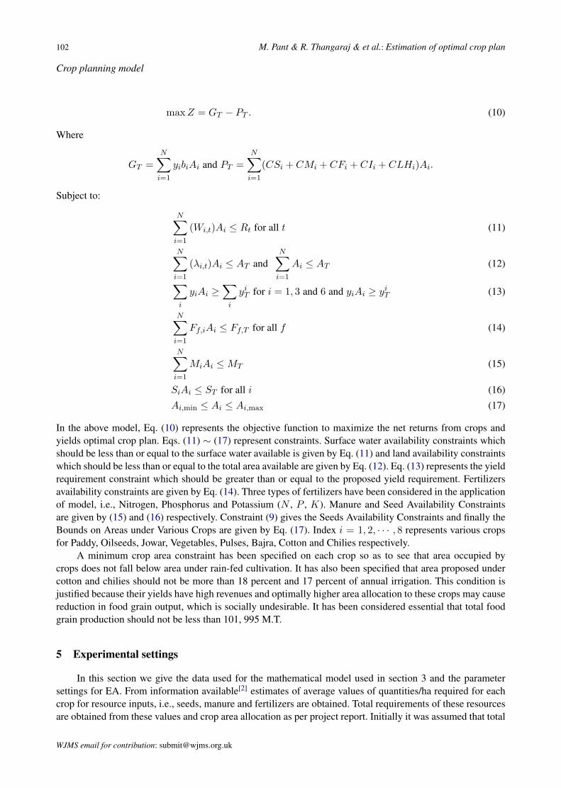
Table 4. Results of all algorithms: 75% water year dependable flow

ITEM DE PSO EP GA LINGOA1 0.001616 0 0.116411 1986.13 0A2 15233 15233 15232.9 15148.9 15233A3 5034.2 5034.29 5035.25 1232.31 5033.97A4 8124 8124 8123.99 5460.96 8124A5 12186 12186 12186 7155.7 12186.99A6 5193.36 5193.54 5192.15 2948.6 5193.36A7 16000 16000 16000 15933.6 15876.04A8 14624.4 14624.4 14624.4 14570.1 14592.21Z 16503.3 16503.3 16503.3 15731.2 16449.01

Table 5. Results of all algorithms: 50% water year dependable flow

ITEM DE PSO EP GA LINGOA1 0.000198 0 0 128.783 0A2 13125.4 13125.7 13125.7 12634.3 13125.35A3 0.000444 0 0 167.924 0A4 8124 8124 8123.99 7088.14 8124A5 0.000233 0 0 586.484 0A6 927.386 927.889 927.896 683.921 927.3857A7 16000 16000 16000 15699.2 15876.04A8 14624.4 14624.4 14624.4 13507.6 14592.21Z 15319.1 15319.1 15319.1 14455 15264.74

6 Numerical results

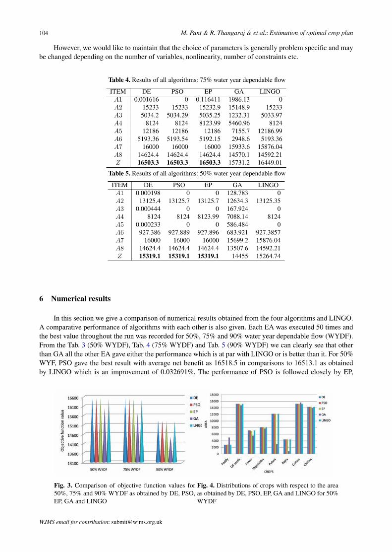
In this section we give a comparison of numerical results obtained from the four algorithms and LINGO.A comparative performance of algorithms with each other is also given. Each EA was executed 50 times andthe best value throughout the run was recorded for 50%, 75% and 90% water year dependable flow (WYDF).From the Tab. 3 (50% WYDF), Tab. 4 (75% WYDF) and Tab. 5 (90% WYDF) we can clearly see that otherthan GA all the other EA gave either the performance which is at par with LINGO or is better than it. For 50%WYF, PSO gave the best result with average net benefit as 16518.5 in comparisons to 16513.1 as obtainedby LINGO which is an improvement of 0.032691%. The performance of PSO is followed closely by EP,

Fig. 3. Comparison of objective function values for50%, 75% and 90% WYDF as obtained by DE, PSO,EP, GA and LINGO

Fig. 4. Distributions of crops with respect to the areaas obtained by DE, PSO, EP, GA and LINGO for 50%WYDF



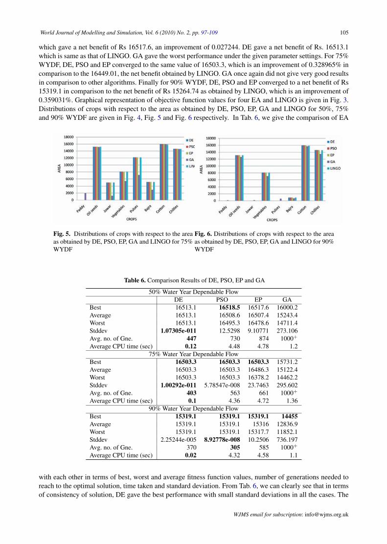
which gave a net benefit of Rs 16517.6, an improvement of 0.027244. DE gave a net benefit of Rs. 16513.1which is same as that of LINGO. GA gave the worst performance under the given parameter settings. For 75%WYDF, DE, PSO and EP converged to the same value of 16503.3, which is an improvement of 0.328965% incomparison to the 16449.01, the net benefit obtained by LINGO. GA once again did not give very good resultsin comparison to other algorithms. Finally for 90% WYDF, DE, PSO and EP converged to a net benefit of Rs15319.1 in comparison to the net benefit of Rs 15264.74 as obtained by LINGO, which is an improvement of0.359031%. Graphical representation of objective function values for four EA and LINGO is given in Fig. 3.Distributions of crops with respect to the area as obtained by DE, PSO, EP, GA and LINGO for 50%, 75%and 90% WYDF are given in Fig. 4, Fig. 5 and Fig. 6 respectively. In Tab. 6, we give the comparison of EA



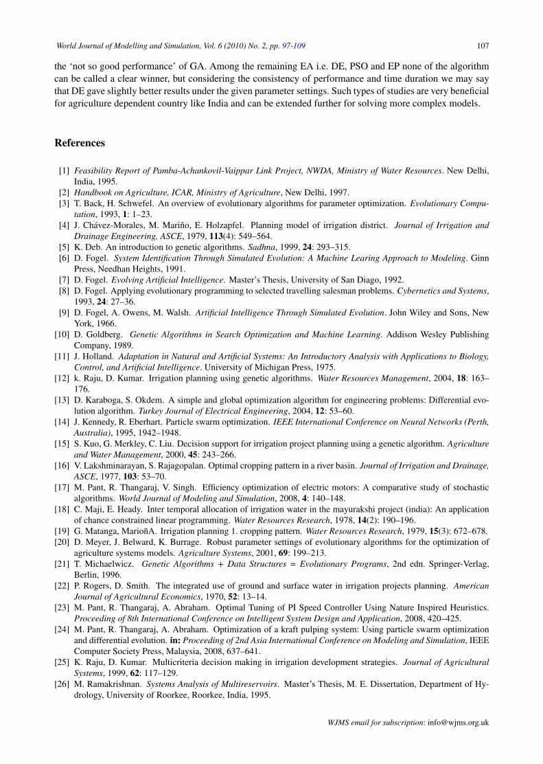
Table 6. Comparison Results of DE, PSO, EP and GA

50% Water Year Dependable FlowDE PSO EP GA

Best 16513.1 16518.5 16517.6 16000.2Average 16513.1 16508.6 16507.4 15243.4Worst 16513.1 16495.3 16478.6 14711.4Stddev 1.07305e-011 12.5298 9.10771 273.106Avg. no. of Gne. 447 730 874 1000+

Average CPU time (sec) 0.12 4.48 4.78 1.275% Water Year Dependable Flow

Best 16503.3 16503.3 16503.3 15731.2Average 16503.3 16503.3 16486.3 15122.4Worst 16503.3 16503.3 16378.2 14462.2Stddev 1.00292e-011 5.78547e-008 23.7463 295.602Avg. no. of Gne. 403 563 661 1000+

Average CPU time (sec) 0.1 4.36 4.72 1.3690% Water Year Dependable Flow

Best 15319.1 15319.1 15319.1 14455Average 15319.1 15319.1 15316 12836.9Worst 15319.1 15319.1 15317.7 11852.1Stddev 2.25244e-005 8.92778e-008 10.2506 736.197Avg. no. of Gne. 370 305 585 1000+

Average CPU time (sec) 0.02 4.32 4.58 1.1

with each other in terms of best, worst and average fitness function values, number of generations needed toreach to the optimal solution, time taken and standard deviation. From Tab. 6, we can clearly see that in termsof consistency of solution, DE gave the best performance with small standard deviations in all the cases. The



best and worst values of GA fluctuated the most and highest deviation was recorded for it. On comparing thetime taken (in sec) we see that DE took minimum time by taking fraction of a second for reaching the optimalsolution, followed by GA, whereas EP and PSO took relatively more time. Also in terms of average numberof generations, DE gave the best performance for 50% and 75% WYDF, followed by PSO and EP. For 90%WYDF, PSO took 305 average numbers of generations followed by DE which took 370 average numbers ofgenerations. The convergence graphs of average number of generations vs. objective function value for 50%,75% and 90% WYDF with respect to DE, PSO and EP are also shown in Fig. 7 ∼ Fig. 9. In all the cases GAtook more than 1000 average numbers generations to reach to the solution and hence it is not depicted in theconvergence graphs.

Fig. 7. Convergence graph for objective function valuevs. number of generations as obtained by DE, PSO andEP with 50% WYDF

Fig. 8. Convergence graph for objective function valuevs. number of generations as obtained by DE, PSO andEP with 75% WYDF

Fig. 9. Convergence graph for objective function value vs. number of generations as obtained by DE, PSO and EP with90% WYDF

7 Conclusion

The present article deals with developing an optimal crop plan model for the command area of PAV linkproject, Kerela, India. The mathematical model of the problem is linear in nature subject to various constraints.For optimal releases made from reservoir using a multi-reservoir operation model, optimal crop plans are de-veloped under adequate, normal and limited irrigation water defined by 50 percent, 75 percent and 90 percentwater year dependable flows, respectively. The optimization model is solved using four popular EvolutionaryAlgorithms; Genetic algorithm, Particle Swarm Optimization, Differential Evolution and Evolutionary Pro-gramming and also with LINGO, a software commonly used for solving LPP models. The performance ofEA is compared with the performance of LINGO and also with each other. Simulation results show that PSO,DE and EP gave a better or at par performance within a satisfactory time frame in comparison to LINGO.Surprisingly GA, which has been most frequently advocated for solving such types of problems didn’t givesatisfactory results in comparison to LINGO and other EA. However we are making further investigations on



the ‘not so good performance’ of GA. Among the remaining EA i.e. DE, PSO and EP none of the algorithmcan be called a clear winner, but considering the consistency of performance and time duration we may saythat DE gave slightly better results under the given parameter settings. Such types of studies are very beneficialfor agriculture dependent country like India and can be extended further for solving more complex models.

References

[1] Feasibility Report of Pamba-Achankovil-Vaippar Link Project, NWDA, Ministry of Water Resources. New Delhi,India, 1995.

[2] Handbook on Agriculture, ICAR, Ministry of Agriculture, New Delhi, 1997.[3] T. Back, H. Schwefel. An overview of evolutionary algorithms for parameter optimization. Evolutionary Compu-

tation, 1993, 1: 1–23.[4] J. Chavez-Morales, M. Marino, E. Holzapfel. Planning model of irrigation district. Journal of Irrigation and

Drainage Engineering, ASCE, 1979, 113(4): 549–564.[5] K. Deb. An introduction to genetic algorithms. Sadhna, 1999, 24: 293–315.[6] D. Fogel. System Identification Through Simulated Evolution: A Machine Learing Approach to Modeling. Ginn

Press, Needhan Heights, 1991.[7] D. Fogel. Evolving Artificial Intelligence. Master’s Thesis, University of San Diago, 1992.[8] D. Fogel. Applying evolutionary programming to selected travelling salesman problems. Cybernetics and Systems,

1993, 24: 27–36.[9] D. Fogel, A. Owens, M. Walsh. Artificial Intelligence Through Simulated Evolution. John Wiley and Sons, New

York, 1966.[10] D. Goldberg. Genetic Algorithms in Search Optimization and Machine Learning. Addison Wesley Publishing

Company, 1989.[11] J. Holland. Adaptation in Natural and Artificial Systems: An Introductory Analysis with Applications to Biology,

Control, and Artificial Intelligence. University of Michigan Press, 1975.[12] k. Raju, D. Kumar. Irrigation planning using genetic algorithms. Water Resources Management, 2004, 18: 163–

176.[13] D. Karaboga, S. Okdem. A simple and global optimization algorithm for engineering problems: Differential evo-

lution algorithm. Turkey Journal of Electrical Engineering, 2004, 12: 53–60.[14] J. Kennedy, R. Eberhart. Particle swarm optimization. IEEE International Conference on Neural Networks (Perth,

Australia), 1995, 1942–1948.[15] S. Kuo, G. Merkley, C. Liu. Decision support for irrigation project planning using a genetic algorithm. Agriculture

and Water Management, 2000, 45: 243–266.[16] V. Lakshminarayan, S. Rajagopalan. Optimal cropping pattern in a river basin. Journal of Irrigation and Drainage,

ASCE, 1977, 103: 53–70.[17] M. Pant, R. Thangaraj, V. Singh. Efficiency optimization of electric motors: A comparative study of stochastic

algorithms. World Journal of Modeling and Simulation, 2008, 4: 140–148.[18] C. Maji, E. Heady. Inter temporal allocation of irrigation water in the mayurakshi project (india): An application

of chance constrained linear programming. Water Resources Research, 1978, 14(2): 190–196.[19] G. Matanga, MarionA. Irrigation planning 1. cropping pattern. Water Resources Research, 1979, 15(3): 672–678.[20] D. Meyer, J. Belward, K. Burrage. Robust parameter settings of evolutionary algorithms for the optimization of

agriculture systems models. Agriculture Systems, 2001, 69: 199–213.[21] T. Michaelwicz. Genetic Algorithms + Data Structures = Evolutionary Programs, 2nd edn. Springer-Verlag,

Berlin, 1996.[22] P. Rogers, D. Smith. The integrated use of ground and surface water in irrigation projects planning. American

Journal of Agricultural Economics, 1970, 52: 13–14.[23] M. Pant, R. Thangaraj, A. Abraham. Optimal Tuning of PI Speed Controller Using Nature Inspired Heuristics.

Proceeding of 8th International Conference on Intelligent System Design and Application, 2008, 420–425.[24] M. Pant, R. Thangaraj, A. Abraham. Optimization of a kraft pulping system: Using particle swarm optimization

and differential evolution. in: Proceeding of 2nd Asia International Conference on Modeling and Simulation, IEEEComputer Society Press, Malaysia, 2008, 637–641.

[25] K. Raju, D. Kumar. Multicriteria decision making in irrigation development strategies. Journal of AgriculturalSystems, 1999, 62: 117–129.

[26] M. Ramakrishnan. Systems Analysis of Multireservoirs. Master’s Thesis, M. E. Dissertation, Department of Hy-drology, University of Roorkee, Roorkee, India, 1995.



[27] D. Rani. Multilevel Optimization of a Water Resources System. Master’s Thesis, Department of Mathematics,Indian Institude of Technology, Roorkee, India, 2004.

[28] R. Storn, K. Price. Differential evolution–A simple and efficient adaptive scheme for global optimization overcontinuous spaces. Technical Report, International Computer Science Institute, 1995.

[29] R. Storn, K. Price. Differential evolution–a simple and efficient heuristic for global optimization over continuousspaces. Journal Global Optimization, 1997, 11: 341–359.

[30] J. Windsor, V. Chow. Model of farm irrigation in humid areas. Journal of the Irrigation and Drainage Division,American Society of Civil Engineers, 97 (IR3), 1971, 369–385.

[31] B. Zhang, S. Yuan, et al. Study of corn optimization irrigation model by genetic algorithm. IFIP InternationalFederation for Information Processing 258, Computer and Computing Technologies in Ariculture, 2008, 1: 121–132.

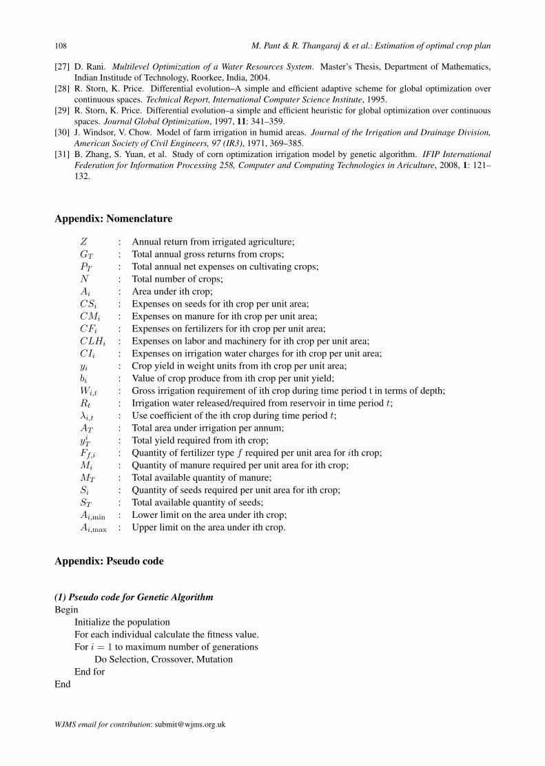
Appendix: Nomenclature

Z : Annual return from irrigated agriculture;GT : Total annual gross returns from crops;PT : Total annual net expenses on cultivating crops;N : Total number of crops;Ai : Area under ith crop;CSi : Expenses on seeds for ith crop per unit area;CMi : Expenses on manure for ith crop per unit area;CFi : Expenses on fertilizers for ith crop per unit area;CLHi : Expenses on labor and machinery for ith crop per unit area;CIi : Expenses on irrigation water charges for ith crop per unit area;yi : Crop yield in weight units from ith crop per unit area;bi : Value of crop produce from ith crop per unit yield;Wi,t : Gross irrigation requirement of ith crop during time period t in terms of depth;Rt : Irrigation water released/required from reservoir in time period t;λi,t : Use coefficient of the ith crop during time period t;AT : Total area under irrigation per annum;yi

T : Total yield required from ith crop;Ff,i : Quantity of fertilizer type f required per unit area for ith crop;Mi : Quantity of manure required per unit area for ith crop;MT : Total available quantity of manure;Si : Quantity of seeds required per unit area for ith crop;ST : Total available quantity of seeds;Ai,min : Lower limit on the area under ith crop;Ai,max : Upper limit on the area under ith crop.

Appendix: Pseudo code

(1) Pseudo code for Genetic AlgorithmBegin

Initialize the populationFor each individual calculate the fitness value.For i = 1 to maximum number of generations

Do Selection, Crossover, MutationEnd for

End



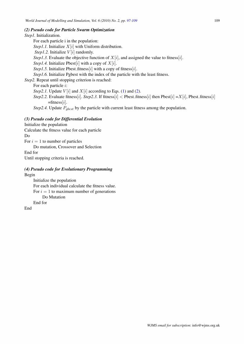
(2) Pseudo code for Particle Swarm OptimizationStep1. Initialization.

For each particle i in the population:Step1.1. Initialize X[i] with Uniform distribution.Step1.2. Initialize V [i] randomly.Step1.3. Evaluate the objective function of X[i], and assigned the value to fitness[i].Step1.4. Initialize Pbest[i] with a copy of X[i].Step1.5. Initialize Pbest fitness[i] with a copy of fitness[i].Step1.6. Initialize Pgbest with the index of the particle with the least fitness.

Step2. Repeat until stopping criterion is reached:For each particle i:Step2.1. Update V [i] and X[i] according to Eqs. (1) and (2).Step2.2. Evaluate fitness[i]. Step2.3. If fitness[i] < Pbest fitness[i] then Pbest[i] =X[i], Pbest fitness[i]

=fitness[i].Step2.4. Update Pgbest by the particle with current least fitness among the population.

(3) Pseudo code for Differential EvolutionInitialize the populationCalculate the fitness value for each particleDoFor i = 1 to number of particles

Do mutation, Crossover and SelectionEnd forUntil stopping criteria is reached.

(4) Pseudo code for Evolutionary ProgrammingBegin

Initialize the populationFor each individual calculate the fitness value.For i = 1 to maximum number of generations

Do MutationEnd for

End


estimation of optimal crop plan using nature inspired ... of optimal crop plan using nature inspired...

Documents