APPLIED AND ENVIRONMENTAL MICROBIOLOGY, Aug. 1989, p. 1934-19420099-2240/89/081934-09$02.00/0Copyright © 1989, American Society for Microbiology

Estimation of Microbial Densities from Dilution Count ExperimentsCHARLES N. HAAS

Pritzker Department of Environmental Engineering, Illinois Institute of Technology, Chicago, Illinois 60616

Received 22 December 1988/Accepted 8 May 1989

Although dilution counts have been widely used in quantitative microbiology, their interpretation has alwaysbeen widely discussed both in microbiology and in applied statistics. Maximum-likelihood (most-probable-number) methods have generally been used to estimate densities from dilution experiments. It has not beenwidely recognized that these methods are intrinsically and statistically biased at the sample sizes used inmicrobiology. This paper presents an analysis of proposed method for correction of such biases, and themethod was found to be robust for moderate deviations from Poisson behavior. For analyses at greater variancewith the Poisson assumptions, the use of the Spearman-Karber method is analyzed and shown to yield anestimate of density of lesser bias than that produced by the most-probable-number method. Revised methodsof constructing confidence limits proposed by Loyer and Hamilton (M. W. Loyer and M. A. Hamilton,Biometrics 40:907-916, 1984) are also discussed, and charts for the three- and four- decimal dilution series withfive tubes per dilution are presented.

The use of dilution counts for the determination of micro-bial densities has a long history in applied microbiology. Insuch a technique, a number of tubes are inoculated withvarious dilutions of a suspension containing microorgan-isms. Under the assumption of random sampling of enumer-able units, leading to a Poisson probability distribution forthe expected number of organisms inoculated in a givenvolume, the density of the original suspension can be esti-mated by using the maximum-likelihood technique (3, 10, 22,23).

It has been known for many years, however, that themaximum-likelihood technique leads to biased estimates forparameters in all but the most simple cases (11, 15, 18).Indeed, in early comparisons of the membrane filter andmost-probable-number (MPN) coliform techniques, the ten-dency for a positive bias in the MPN method was noted (20).Only more recently, however, has a method become avail-able for the first-order correction of the inherent positivebias of this technique (17). In a related area, the estimation ofconfidence limits for MPN determinations has been reexam-ined by Loyer and Hamilton (14), who present alternativeand more statistically rigorous methods for addressing thisproblem than those presently used in environmental micro-biology (22).Any procedure for the analysis of dilution experiments

must be reasonably robust to the possible presence ofdeviations from the Poisson assumption. For example, a

number of studies have indicated that replicate counts inenvironmental samples might be distributed according to thenegative binomial, rather than the Poisson, distribution (2, 6,8, 9, 16). The negative binomial distribution is an example ofa discrete distribution with variance in excess of the Pois-son-termed an overdisperse distribution. Such variancemay be intrinsic to the enumeration methodology itself andthus may be experimentally correctable; one example of thistype of situation is a possible variation in the efficiency ofrecovery between tubes. Alternatively, the variation may bea property of the microbial population itself. For example, iforganisms exist in clumps possessing a frequency distribu-tion of organisms per clump, and if clumps are randomlysampled but a dislodgement occurs during handling, thedistribution of viable units will probably be overdisperse. Ifthe latter type of situation forms the basis for the overdis-

persion, some method of analysis of dilution count datarobust to the overdispersion is required.

It is the objective of this paper to explore the utility of thebias correction method and the alternative methods forconstructing confidence limits to the common dilution seriesused in MPN determinations. First, the more recent tech-niques are examined and are found to be relatively robust forsmall to moderate deviations from the underlying assump-tions of Poisson distribution of replication error. Then,alternatives methodologies for use when the replication erroris severely different from Poisson are developed. In workpreviously published, diagnostic methods for detecting de-viations from the Poisson distribution are presented (9).

MATERIALS AND METHODS

Likelihood estimation. If dilutions 1 through r, each with nrtubes (not necessarily equal), are inoculated with a volumeVr of sample from a material containing an average concen-tration of microorganisms p,, standard theory (3) shows thatthe probability that a random vector (P1, P2.... Pr) ofpositive tubes will be observed is given by the followingequation:

(1)L= E (ni pi)!p! !(p0,)i Pi(l _ Po0i)Pii~

with

pO.i e-Vi (2)Equation 2 results from an independent Poisson distributionat each dilution for the distribution of microorganisms in a

single volume of inoculum, and equation 1 expresses theindependence of each replication and each dilution. If pu isknown, L is the probability that a given combination ofpositive tubes will be obtained. If is unknown, the maxi-mum-likelihood estimate (MLE) of its value can be obtainedby finding the value of which, for the observed tubescores, maximize the value of L (termed the likelihood).Should the sample be drawn under circumstances where

the Poisson distribution does not apply, equation 1 can stillbe used to compute the probability that a given set of tubescores were obtained given the true distribution (and param-

1934

Vol. 55, No. 8

on June 20, 2018 by guesthttp://aem

.asm.org/

Dow

nloaded from

DILUTION COUNT DENSITY ESTIMATION 1935

eters of the distribution). However, in this case, equation 2will be replaced by an alternative relationship for the prob-ability of having no organisms in an inoculum. For example,if the distribution is negative binomial, the relationship willbecome

Po= (1 + p.Vlk)I-k (3)with k being the dispersion parameter of the negative bino-mial distribution. The negative binomial distribution hasbeen used to describe microbial distributions in which thevariance between replicates is in excess of the Poissondistribution (2, 6, 16). As k increases to infinity, the negativebinomial distribution approaches the Poisson distribution.

If a Poisson distribution is used to formulate the likelihoodequation for an MLE of a sample drawn from a populationwhich is, in fact, negative binomial, a systematic error in theMLE will result. Wadley (21) first noted that, for a singledilution (r = 1), the erroneous use of a Poisson assumptionnegatively biases the estimate of microbial densities ofsamples from negative binomially distributed populations.Bias is defined as the expected value of p. minus its truevalue. However, the robustness of the MLE (as well as tobias-corrected MLEs) to deviations from the Poisson as-sumption when r > 1 has not, apparently, been explored.

Bias correction methodology. Standard statistical theorypredicts that the MLE estimator of the mean of a Poissonpopulation should, for a sufficiently large number of samples(large nr), approach the true mean at a rate proportional tollnr. However, in usual practice, nr is not large, and bias inthe estimator is to be expected. Salama et al. (17) havepresented a method for correcting the bias to order llnr2.However, these authors did not present the application oftheir method to the typical five-tube decimal dilution seriesused in environmental microbiology, nor did they examinethe robustness of their correction to deviations from thePoisson assumption.The correction derived by Salama et al. (17) is essentially

a Taylor series expansion. If ,u* is the maximum likelihoodestimator of microbiol density, a bias-corrected densityestimator (p.) is given by the following equation:

r 2Rp * (1/2) E (2 nie - *V(l -eL*Vi)

with

d2, v,2 rvEVJzjsinh(R*Vj)laxi2 2(1 - e Vi)2D3 1[cosh(*Vj)-

(1 - e - > Vl)cosh(p.* Vi) - 1ID2

zj = n1(l - e- "*V)

r VJ2ZjD= Ejj

i = 12[cosh(R* Vj) - 1]Distribution-free estimation of densities. The problem of

estimating the central point (50% effective dose or 50% lethalconcentration) of a bioassay has been a longstanding one inbiology and statistics. The MPN technique can be regardedas a bioassay with the ED50 being related to the microbialdensity. In particular, one can assume an underlying toler-

ance distribution (logit or probit) and use the method ofmaximum likelihood to estimate the median of this distribu-tion (4). Alternatively, by using a variety of distribution-freemethods, one can form estimates of the median of theempirical bioassay curve (1, 7, 12, 13). Distribution-freemethods, although frequently less precise than other meth-ods (in the statistical sense of producing greater estimatingvariance when the underlying assumptions are true), arevery often insufficiently robust (being highly sensitive todeviations from the underlying assumptions).One of the most widely used methods for producing a

distribution-free estimate of the 50% effective concentrationis the Spearman-Karber method (7, 12). In this work, theSpearman-Karber method is applied to locate the volumewhich is capable of infecting 50% of the dilution tubes. Thereciprocal of this volume is defined as the Spearman-Karber(SK) estimate of microbial density. The procedure for con-struction of this estimate, given an MPN experiment inwhich sets of Ttubes are exposed to a series of volumes (Vl,V2, ..., V, with V1 > V2, etc.) producing positives (infectedtubes) P1, ..., P, is as follows. (i) A transformed doseparameter is computed to make the infectivity curve moresymmetrical. In bioassay work, log-transforms are common(see, e.g., reference 12). In this work, the log-transform isused; thus, one computes di = In (V,). Coincidentally, thisalso renders the dose intervals equally spaced on an arith-metic scale (for common dilution sequences) with a separa-tion (di - di + 1) of A. (ii) The series is appended with twofictitious observations designed so that the series continuesfrom complete infection to complete sterility. This proce-dure has no effect if the sequence is already bracketed by 100and 0% infection. Mathematically,

do = d1 + A, PO = Td + = dn- A, Pn+l = 0

(iii) Frequencies of positives are computed at each dose; i.e.,fi = P/T. (iv) The frequencies of positives are adjusted toproduce a monotonically decreasing sequence off s. For anyi, if fti > fi - 1, new frequencies (fI) are defined by

ri =ffi- = (1/2)(fi + f-1);after replacing thef s by thefJ's, the process continues untilthe entire sequence is monotonic (12). (v) The SK estimate isthen obtained by the following computation, which amountsto an integration of the dose-response polygon:

Q = E(f3 -f + 1)(dj + dj+ 1)/2j=o

where SK = e-Q.Comparison of point estimators. In this study, the perfor-

mance of the MLE, the bias-corrected MLE estimator, andthe SK estimator were studied by using a four-dilution,five-tube experiment with volumes of 10, 1, 0.1, and 0.01 ml.The range of p. values from 0.01 to 100/ml was subdividedinto 40 intervals equally spaced on a log scale (i.e., log1ointervals of 0.1). For each assumed true p. value, thefrequency of all possible tube scores (i.e., combinations ofpositive and negative tubes) was computed from equation 1.From the tube score, the value of each of the estimators(standard, bias-corrected, and SK) was then computed. Theexpected value of each estimator as a function of p. was thenobtained by summing the products of the value of theestimator for a given tube score and the frequency withwhich that tube score is obtained at the value of p.. Similarly,

VOL. 55, 1989

on June 20, 2018 by guesthttp://aem

.asm.org/

Dow

nloaded from

APPL. ENVIRON. MICROBIOL.

1.5

1.

U1)

\

+-JF-i

Uf)

CL

1.

1.2

1.1_

.0

Correctedi0.0

0.8V.000.001

U0U

0~

ci0U1)

U1)

0

U1)

0.010 0.100 1.000 10.000 100.000

True Meon (I#/mL)FIG. 1. Comparison of expected bias versus true mean for Pois-

son-distributed bacteria by using the MLE and corrected MLEmethods.

the mean square error (MSE) of each estimator as a functionof the true mean was also computed. The MSE is the averageof the sum of the squares of the differences between the truevalue of microbial concentration and its estimate. For thescore (5, 5, 5, 5), the MLE and the bias-corrected MLE wereboth assumed to be 10,000/ml. The MLE estimate wascomputed by a Newton-Raphson iteration method.The performance of the estimators in the presence of

overdispersion was also assessed by using the above proce-dure, in which the negative binomial distribution with a fixedk value was used to determine the tube score frequency viaequations 1 and 3. However, the MLE was determined byusing an assumed Poisson distribution and equations 1 and 2.

Confidence limits to the maximum likelihood estimator. TheSterne method for computing confidence limits (intervalestimates) for the MPN estimator developed by Loyer andHamilton (14) computes the set of tube scores (P1, P2.9 Pr)which lie in a confidence limit by successively, for all valuesof the true density (,u), computing the most frequentlyobserved scores ranked by their frequency. The ot confi-dence limit (e.g., 0.05) for a tube score combination (Pl, P2,. Pr) is defined as the range of I. values for which that score

lies within the (1 - ot) most frequently observed combina-tions. In this study, the confidence limits were determinedby examining the range 0.01 to 1,000/ml over 500 equallyspaced logarithmic intervals (log1o intervals of 0.01) for pL.

The Woodward method (22) by which confidence limits ofmost frequent use in sanitary microbiology have been ob-tained assumes that the MLE for the observed tube score isthe true mean. The confidence limit for the true meanconsists of the range of the MLE values for the central (1 -

a) proportion of tube scores ranked by their MLE. One ofthe major criticisms of this method (14) is that it frequentlyincludes highly improbable tube scores in the confidenceregion while rejecting more probable scores.

RESULTS

Bias reduction method. For a four-dilution experiment,over the entire range examined, the first-order bias reductionmethod produced point estimates of MPN of lower relativebias (defined as [mean estimator - true value]/true value)(Fig. 1) and MSE (Fig. 2) than the conventional MLE. These

10 0.100 1.000

True Meon (#/mL)100.000

FIG. 2. Comparison of relative MSE (as a fraction of the truemean) for Poisson-distributed bacteria by using the MLE andcorrected MLE methods.

findings are similar to those of Salama et al. (17), whopresented results for other experimental designs.

Prior workers have used a bias correction factor of 85%for the five-tube MPN test (19). The derivation of this factoris obscure, but probably involved an assumption about theunderlying true MPN value itself. Examination of Fig. 1shows that this correction factor is roughly the average ofthe bias over the midrange of microbial densities. It is alsoclear from this figure that over a similar range the bias in thecorrected MLE is substantially less than 5%.

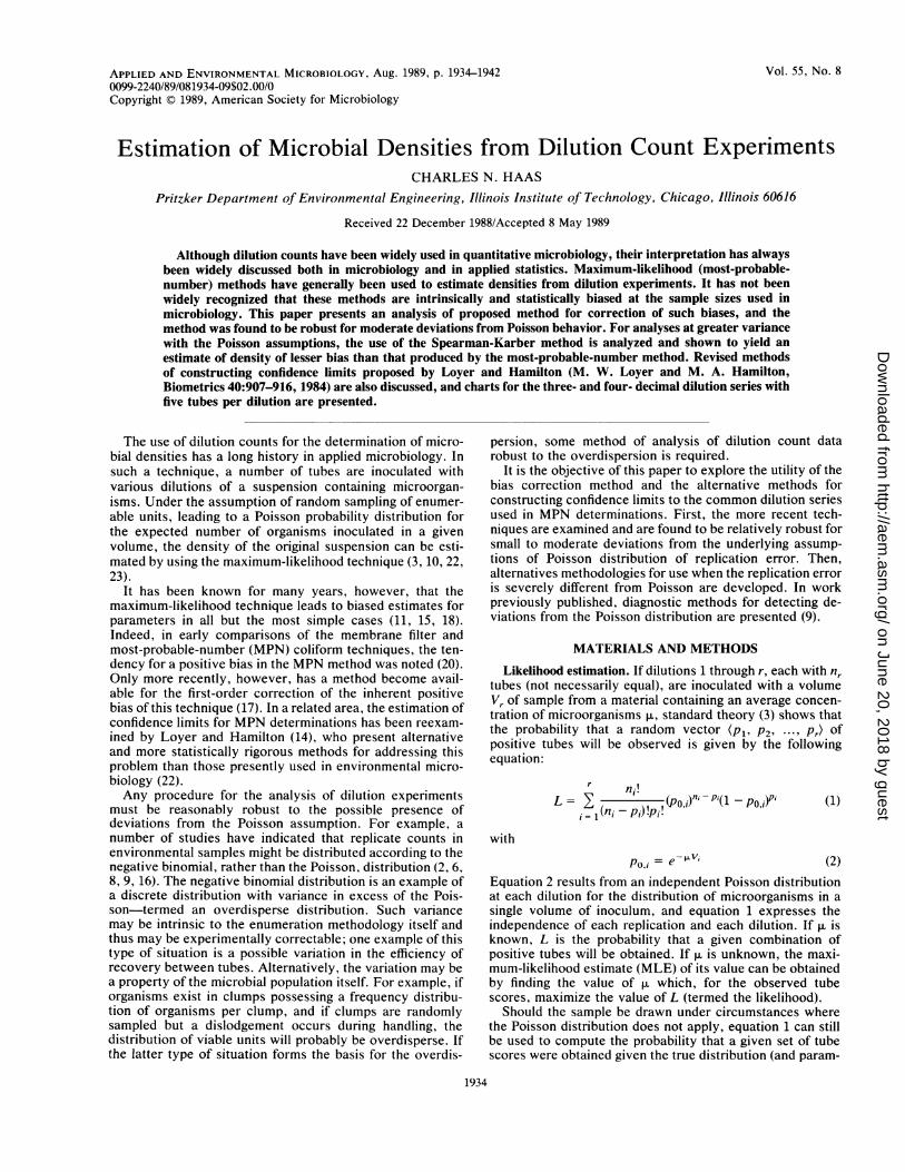
If the average relative bias and MSE are computed overthe midrange of values for for negative binomial distribu-tions of various degrees of dispersion (k values), it is foundthat the bias-corrected estimator is still superior to the MLE,provided that the negative binomial k value is greater than6.0 (Fig. 3 and 4). Since tests are available to detectdeviations from Poisson behavior which are sensitive tonegative binomial k values at this level with sample sizes ofabout 1,000 (9), the correction for bias appears to be usefulin conjunction with tests of homogeneity to confirm consis-tency with underlying Poisson statistics. This result is in

()

a)

-s-i

0

0

U)b

0.2 1.0 10.0 100.0 300.0

negotive binomiol k volue

FIG. 3. Effect of negative binomial k value on the estimation biasby the MLE and corrected MLE methods.

4 dilution Poisson.4

MLE

1936 HAAS

on June 20, 2018 by guesthttp://aem

.asm.org/

Dow

nloaded from

DILUTION COUNT DENSITY ESTIMATION 1937

L

F-,-0cSao XA

E

C) 0.19

. Co rrec e

0.8 ..............0.001 0.010 0.100 1.000 10.000 100.000

True Meon (#/100 mL)FIG. 4. Estimation bias versus true mean for a negative binomial

distribution with k = 6.

qualitative accord with the results of Wadley (21), who notedthat for single-dilution experiments, a negative binomiallydistributed population would be underestimated if the Pois-son assumption were used to compute an MPN value.

Similar conclusions about the effect of deviation on therelative performance of the MLE versus the correctedmethods were obtained for a five-tube, three-decimal-di-lution experiment (results not shown). Furthermore, thereduction in bias and MSE was about as good in thethree-decimal-dilution protocol as in the four-decimal-di-lution protocol.Based on this analysis, alternative MPN tables for the

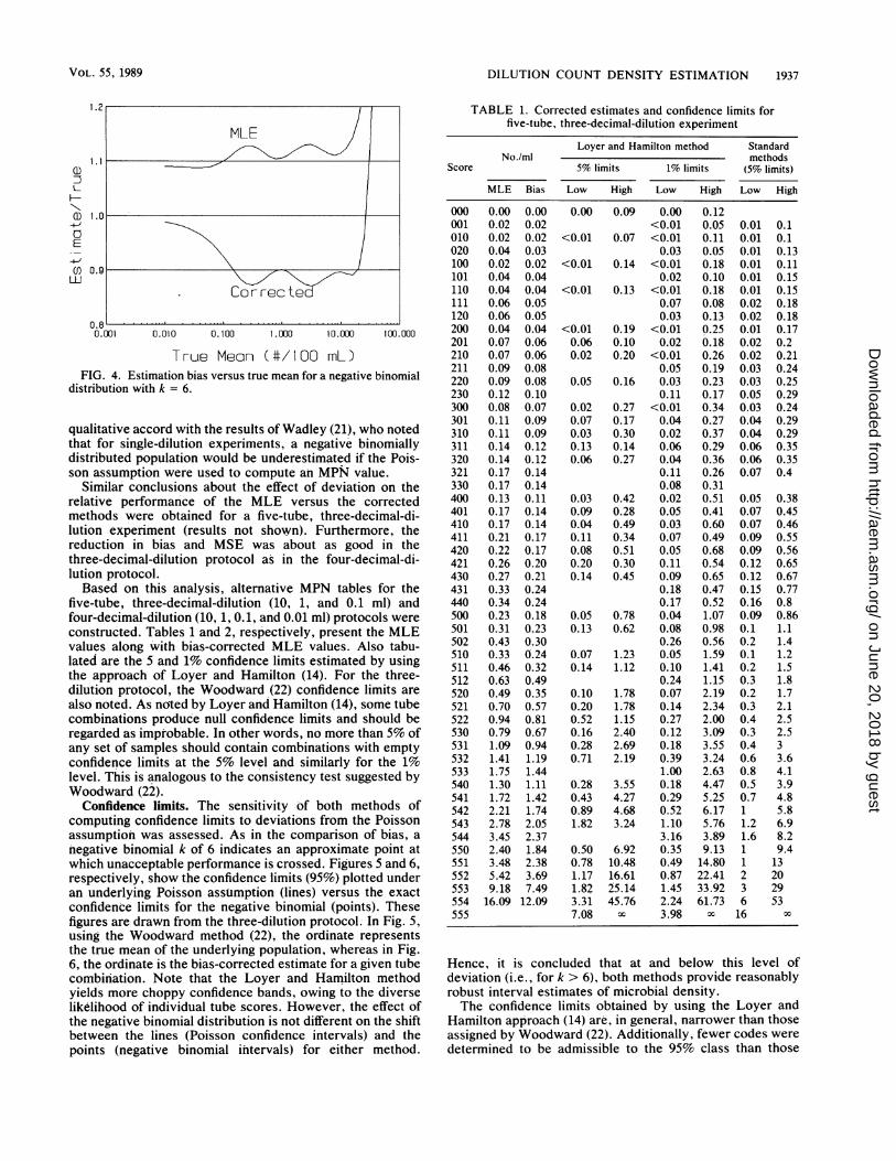
five-tube, three-decimal-dilution (10, 1, and 0.1 ml) andfour-decimal-dilution (10, 1, 0.1, and 0.01 ml) protocols wereconstructed. Tables 1 and 2, respectively, present the MLEvalues along with bias-corrected MLE values. Also tabu-lated are the 5 and 1% confidence limits estimated by usingthe approach of Loyer and Hamilton (14). For the three-dilution protocol, the Woodward (22) confidence limits arealso noted. As noted by Loyer and Hamilton (14), some tubecombinations produce null confidence limits and should beregarded as improbable. In other words, no more than 5% ofany set of samples should contain combinations with emptyconfidence limits at the 5% level atid similarly for the 1%level. This is analogous to the consistency test suggested byWoodward (22).

Confidence limits. The sensitivity of both methods ofcomputing confidence limits to deviations from the Poissonassumption was assessed. As in the comparison of bias, anegative binomial k of 6 indicates an approximate point atwhich unacceptable performance is crossed. Figures 5 and 6,respectively, show the confidence limits (95%) plotted underan underlying Poisson assumption (lines) versus the exactconfidence limits for the negative binomial (points). Thesefigures are drawn from the three-dilution protocol. In Fig. 5,using the Woodward method (22), the ordinate representsthe true mean of the underlying population, whereas in Fig.6, the ordinate is the bias-corrected estimate for a given tubecombination. Note that the Loyer and Hamilton methodyields more choppy confidence bands, owing to the diverselikelihood of individual tube scores. However, the effect ofthe negative binomial distribution is not different on the shiftbetween the lines (Poisson confidence intervals) and thepoints (negative binomial intervals) for either method.

TABLE 1. Corrected estimates and confidence limits forfive-tube, three-decimal-dilution experiment

Score

000001010020100101110111120200201210211220InLJU

300301310311320321330400401410411420421430431440500501502510511512520521522530531532533540541542543544550551552553554555

No./ml

MLE Bias

0.00 0.000.02 0.020.02 0.020.04 0.030.02 0.020.04 0.040.04 0.040.06 0.050.06 0.050.04 0.040.07 0.060.07 0.060.09 0.080.09 0.080.12 0.100.08 0.070.11 0.090.11 0.090.14 0.120.14 0.120.17 0.140.17 0.140.13 0.110.17 0.140.17 0.140.21 0.170.22 0.170.26 0.200.27 0.210.33 0.240.34 0.240.23 0.180.31 0.230.43 0.300.33 0.240.46 0.320.63 0.490.49 0.350.70 0.570.94 0.810.79 0.671.09 0.941.41 1.191.75 1.441.30 1.111.72 1.422.21 1.742.78 2.053.45 2.372.40 1.843.48 2.385.42 3.699.18 7.4916.09 12.09

Loyer and Hamilton method Standardmethods

5% limits 1% limnits

Low High Low High

0.00 0.09 0.00 0.12<0.01 0.05

<0.01 0.07 <0.01 0.110.03 0.05

<0.01 0.14 <0.01 0.180.02 0.10

<0.01 0.13 <0.01 0.180.07 0.080.03 0.13

<0.01 0.19 <0.01 0.250.06 0.10 0.02 0.180.02 0.20 <0.01 0.26

0.05 0.190.05 0.16 0.03 0.23

0.11 0.170.02 0.27 <0.01 0.340.07 0.17 0.04 0.270.03 0.30 0.02 0.370.13 0.14 0.06 0.290.06 0.27 0.04 0.36

0.11 0.260.08 0.31

0.03 0.42 0.02 0.510.09 0.28 0.05 0.410.04 0.49 0.03 0.600.11 0.34 0.07 0.490.08 0.51 0.05 0.680.20 0.30 0.11 0.540.14 0.45 0.09 0.65

0.18 0.470.17 0.52

0.05 0.78 0.04 1.070.13 0.62 0.08 0.98

0.26 0.560.07 1.23 0.05 1.590.14 1.12 0.10 1.41

0.24 1.150.10 1.78 0.07 2.190.20 1.78 0.14 2.340.52 1.15 0.27 2.000.16 2.40 0.12 3.090.28 2.69 0.18 3.550.71 2.19 0.39 3.24

1.00 2.630.28 3.55 0.18 4.470.43 4.27 0.29 5.250.89 4.68 0.52 6.171.82 3.24 1.10 5.76

3.16 3.890.50 6.92 0.35 9.130.78 10.48 0.49 14.801.17 16.61 0.87 22.411.82 25.14 1.45 33.923.31 45.76 2.24 61.737.08 oc 3.98 Xc

(5% limits)

Low High

0.010.010.010.010.010.010.020.020.010.020.020.030.030.050.030.040.040.060.060.07

0.050.070.070.090.090.120.120.150.160.090.10.20.10.20.30.20.30.40.30.40.60.80.50.711.21.61123616

0.10.10.130.110.150.150.180.180.170.20.210.240.250.290.240.290.290.350.350.4

0.380.450.460.550.560.650.670.770.80.861.11.41.21.51.81.72.12.52.533.64.13.94.85.86.98.29.413202953

cc

Hence, it is concluded that at and below this level ofdeviation (i.e., for k > 6), both methods provide reasonablyrobust interval estimates of microbial density.The confidence limits obtained by using the Loyer and

Hamilton approach (14) are, in general, narrower than thoseassigned by Woodward (22). Additionally, fewer codes weredetermined to be admissible to the 95% class than those

VOL. 55, 1989

on June 20, 2018 by guesthttp://aem

.asm.org/

Dow

nloaded from

APPL. ENVIRON. MICROBIOL.

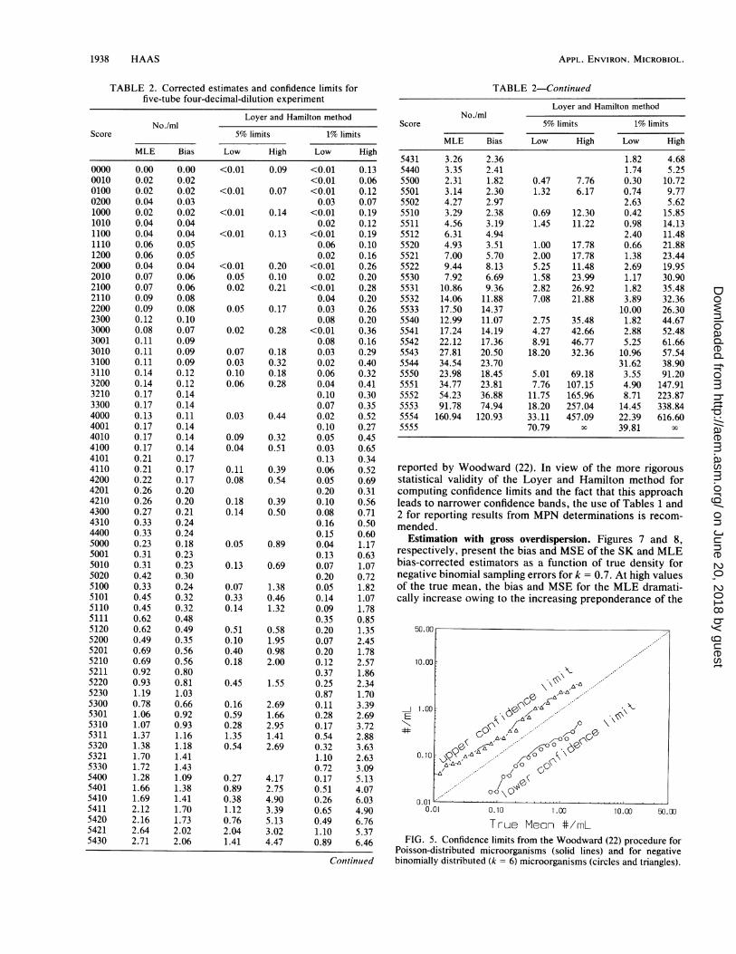
TABLE 2. Corrected estimates and confidence limits forfive-tube four-decimal-dilution experiment

Loyer and Hamilton methodNo./ml

Score 5% limits 1% limits

High Low

0.09 <0.01<0.01

0.07 <0.010.03

0.14 <0.010.02

0.13 <0.010.060.02

0.20 <0.010.10 0.020.21 <0.01

0.040.17 0.03

0.080.28 <0.01

0.080.18 0.030.32 0.020.18 0.060.28 0.04

0.100.07

0.44 0.020.10

0.32 0.050.51 0.03

0.130.39 0.060.54 0.05

0.200.39 0.100.50 0.08

0.160.15

0.89 0.040.13

0.69 0.070.20

1.38 0.050.46 0.141.32 0.09

0.350.58 0.201.95 0.070.98 0.202.00 0.12

0.371.55 0.25

0.872.69 0.111.66 0.282.95 0.171.41 0.542.69 0.32

1.100.72

4.17 0.172.75 0.514.90 0.263.39 0.655.13 0.493.02 1.104.47 0.89

High

0.130.060.120.070.190.120.190.100.160.260.200.280.200.260.200.360.160.290.400.320.410.300.350.520.270.450.650.340.520.690.310.560.710.500.601.170.631.070.721.821.071.780.851.352.451.782.571.862.341.703.392.693.722.883.632.633.095.134.076.034.906.765.376.46

Continued

TABLE 2-Continued

Loyer and Hamilton methodNo./ml

Score 5% limits 1% limits

MLE Bias Low High Low High

5431 3.26 2.36 1.82 4.685440 3.35 2.41 1.74 5.255500 2.31 1.82 0.47 7.76 0.30 10.725501 3.14 2.30 1.32 6.17 0.74 9.775502 4.27 2.97 2.63 5.625510 3.29 2.38 0.69 12.30 0.42 15.855511 4.56 3.19 1.45 11.22 0.98 14.135512 6.31 4.94 2.40 11.485520 4.93 3.51 1.00 17.78 0.66 21.885521 7.00 5.70 2.00 17.78 1.38 23.445522 9.44 8.13 5.25 11.48 2.69 19.955530 7.92 6.69 1.58 23.99 1.17 30.905531 10.86 9.36 2.82 26.92 1.82 35.485532 14.06 11.88 7.08 21.88 3.89 32.365533 17.50 14.37 10.00 26.305540 12.99 11.07 2.75 35.48 1.82 44.675541 17.24 14.19 4.27 42.66 2.88 52.485542 22.12 17.36 8.91 46.77 5.25 61.665543 27.81 20.50 18.20 32.36 10.96 57.545544 34.54 23.70 31.62 38.905550 23.98 18.45 5.01 69.18 3.55 91.205551 34.77 23.81 7.76 107.15 4.90 147.915552 54.23 36.88 11.75 165.96 8.71 223.875553 91.78 74.94 18.20 257.04 14.45 338.845554 160.94 120.93 33.11 457.09 22.39 616.605555 70.79 Xo 39.81 x

reported by Woodward (22). In view of the more rigorousstatistical validity of the Loyer and Hamilton method forcomputing confidence limits and the fact that this approachleads to narrower confidence bands, the use of Tables 1 and2 for reporting results from MPN determinations is recom-mended.

Estimation with gross overdispersion. Figures 7 and 8,respectively, present the bias and MSE of the SK and MLEbias-corrected estimators as a function of true density fornegative binomial sampling errors for k = 0.7. At high valuesof the true mean, the bias and MSE for the MLE dramati-cally increase owing to the increasing preponderance of the

t#

10.00 50.00

True Meon #/mLFIG. 5. Confidence limits from the Woodward (22) procedure for

Poisson-distributed microorganisms (solid lines) and for negativebinomially distributed (k = 6) microorganisms (circles and triangles).

0000001001000200100010101100111012002000201021002110220023003000300130103100311032003210330040004001401041004101411042004201421043004310440050005001501050205100510151105111512052005201521052115220523053005301531053115320532153305400540154105411542054215430

MLE Bias

0.00 0.000.02 0.020.02 0.020.04 0.030.02 0.020.04 0.040.04 0.040.06 0.050.06 0.050.04 0.040.07 0.060.07 0.060.09 0.080.09 0.080.12 0.100.08 0.070.11 0.090.11 0.090.11 0.090.14 0.120.14 0.120.17 0.140.17 0.140.13 0.110.17 0.140.17 0.140.17 0.140.21 0.170.21 0.170.22 0.170.26 0.200.26 0.200.27 0.210.33 0.240.33 0.240.23 0.180.31 0.230.31 0.230.42 0.300.33 0.240.45 0.320.45 0.320.62 0.480.62 0.490.49 0.350.69 0.560.69 0.560.92 0.800.93 0.811.19 1.030.78 0.661.06 0.921.07 0.931.37 1.161.38 1.181.70 1.411.72 1.431.28 1.091.66 1.381.69 1.412.12 1.702.16 1.732.64 2.022.71 2.06

Low

<0.01

<0.01

<0.01

<0.01

<0.010.050.02

0.05

0.02

0.070.030.100.06

0.03

0.090.04

0.110.08

0.180.14

0.05

0.13

0.070.330.14

0.510.100.400.18

0.45

0.160.590.281.350.54

0.270.890.381.120.762.041.41

1938 HAAS

on June 20, 2018 by guesthttp://aem

.asm.org/

Dow

nloaded from

DILUTION COUNT DENSITY ESTIMATION 1939

UU1 ,- W y ;/' .AI>C;-"~~~~A 6\=t4=~~~~~~~~~~~~~0/

0. 10 ~ CAI/

0.01"0.01 1O.0 1.00 10.00 50.00

correcited estimote (#/mL)FIG. 6. Confidence limits from the Loyer and Hamilton (14)

procedure for Poisson-distributed microorganisms (solid lines) andfor negative binomially distributed (k = 6) microorganisms (circlesand triangles).

score (5, 5, 5, 5). However, the SK estimator is less sensitiveto this score (owing to the bracketing of the sequence,effectively converting it to the sequence (5, 5, 5, 5, 5, 0)). Inthe range of intermediate densities, it is clear that the SKestimator is substantially less biased than the MLE. TheMSE is not substantially greater for the SK estimator thanfor the MLE in this broad intermediate range (Table 3).From a more global perspective, the average values of the

relative bias and the relative MSE over true densities of 0.02to 20/ml are shown in Fig. 9 and 10. It is clear that the SKestimator leads to a lowered MSE (Fig. 10) over the entirerange of k values studied (0.3 to 256). Furthermore, as the kvalue decreases and deviations from the Poisson assumptionincrease, the reduction in MSE becomes more pronounced.With respect to bias, below a k value of approximately 1, theabsolute value of mean relative bias is less for the SKestimator than for the MLE (and, although not shown, alsofor the bias-corrected MLE).

Nonetheless, there is significant negative bias for allestimators studied at low values of the negative binomial k(and high degrees of excess dispersion relative to the Poisson

0.4

m 0.2 s

.-' -0.2

- -0.4 0ILEDGil _n

0.01 0.10 1.00 10.00 100.00

True Mean ( /mL )FIG. 7. Relative bias for various estimators with an underlying

negative binomial distribution (k = 0.7).

CfO)

1 .2

0.

0.84

0.4 . .. . ..0.01 0.10 1.00 10.00 100.00

True eon (#/ 100 mL)FIG. 8. Relative MSE for various estimators with an underlying

negative binomial distribution (k = 0.7).

distribution). Thus, further research is desirable to exploremeans of reducing this bias at high overdispersions.The tendency of the SK estimator to produce results in

excess of the MLE is probably a direct consequence of theassumption that the observed sequence is bracketed bycomplete infection (at the next highest volume) and completesterility (at the next lowest volume), thus introducing a slightpositive bias (4). The reasonable performance of the SKestimator for assessing negative binomial means stems fromthe consistency of the negative binomial distribution with theunderlying assumptions in the range 0.1 < k < 1. Thetolerance distribution can be written as follows:

P = [1 + exp(QD)/kf-kwhere 1 = log p.V.

Table 4 presents the mean and median values of cP forvarious values of k. The closeness of the mean and themedian down to k = 0.2 (where they are within 0.3 log unit,or a factor of 2) indicates the existence of a reasonablysymmetric distribution. Furthermore, a k < 1, the medianvalue of 1) is positive; hence, by the above definition, thetrue mean (p.) would be greater than that estimated by the

1 .2

0.6-0)

CD o.o LDE C.4r 00c

0.1 1.0 10.0k vo ILie

FIG. 9. Average relative bias (0.02 to 20/ml true density) versusnegative binomial k value.

VOL. 55, 1989

on June 20, 2018 by guesthttp://aem

.asm.org/

Dow

nloaded from

APPL. ENVIRON. MICROBIOL.

5.0

0

MLE Bios

En>1

DI/OK,- /X

0.5~~~~~~

O. .0 10.0

k volueFIG. 10. Average relative MSE (0.02 to 20/ml true density)

versus negative binomial k value.

reciprocal of the Spearman Karber volume for 50% infectedtubes. In other words, the tendency to a negative bias as kdecreases is a direct outcome of the tolerance distribution.On the basis of this analysis, it is concluded that for

negative binomial deviations leading to k .1.0, the SKestimator is a better indicator of microbial densities than isthe MLE. Although the SK estimator can readily be com-puted by hand, for convenience, Table 3 presents values forvarious tube combinations. For comparison, the MLE esti-mator is also tabulated.

DISCUSSION

The tables presented in this paper can be used as is, assubstitutes for the usual MPN tables, in the analysis of datafrom dilution count experiments. For other tube combina-tions, the procedures discussed above can be used to con-struct alternative tables. The use of these tables is illustratedby an example. Assume that 10 replicate analyses, eachusing a four-decimal-dilution, five-tube protocol, have beenperformed on each of three different water samples. All threewater samples have a mean density of 0.15/ml. However,one water sample has a Poisson distribution of microorgan-isms, whereas the other two have negative binomial distri-butions with k = 1.0 and 0.4. Table 5 indicates the tubescores recorded from each set of samples (at volumes of 10,1, 0.1, and 0.01 ml). Each set of tube scores was a randomsample, given the assumed distribution.The first step is to use Table 2 (to four significant figures)

to obtain, from each tube score, the MLE and the bias-corrected estimates, along with the 95% confidence limitsfrom the Sterne procedure. The SK estimates for each tubescore are obtained from Table 3. It is noted, first, that one ofthe tube scores for the negative binomial (k = 0.4) case,0200, has no confidence limits. This indicates that this tubescore is rare (not appearing in the 95% most frequent set ofscores at any value of >). With only 10 observations, littlecan be done; however, if such a rate of infrequent samplesappeared consistently in a larger data set, a just reason forrejecting the consistency with the Poisson assumption wouldbe provided.When the three methods are used, the conclusions noted

above are seen. The average of the bias-corrected MPN inthe case of the true Poisson distribution is much closer to thetrue value than the MLE itself. However, in the case of the

TABLE 3. SK method for estimating densities in four-dilution,five-tube protocol

Estimated no./ml Estimated no./mlScore Score

MLE SK MLE SK

00000010010002001000101011001110120020002010210021102200230030003001301031003110320032103300400040014010410041014110420042014210430043104400500050015010502051005101511051115120

0.00000.01800.01820.03670.01980.03990.04020.06060.06120.04460.06760.06830.09200.09300.11880.07770.10540.10550.10690.13630.13820.16940.17190.12730.16520.16540.16850.21070.21110.21560.26320.26380.27010.32500.33410.23030.31110.31240.42390.32740.44990.45290.61970.6249

0.03160.05010.05010.07940.05010.07940.07940.12590.12590.07940.12590.12590.19950.19950.31620.12590.19950.19950.19950.31620.31620.50120.50120.19950.31620.31620.31620.50120.50120.50120.79430.79430.79431.25891.25890.31620.50120.50120.79430.50120.79430.79431.25891.2589

520052015210521152205230530053015310531153205321533054005401541054115420542154305431544055005501550255105511551255205521552255305531553255335540554155425543554455505551555255535554

0.48900.68510.69200.92210.93221.18960.78201.05701.07091.36511.38421.69631.72161.27561.65771.68882.11612.16092.64422.70843.25973.35122.31163.13914.26653.29064.56196.30854.93226.99649.43517.924310.864514.055717.497912.993417.238222.115927.809734.543723.979034.766854.225691.7842160.9442

0.79431.25891.25891.99531.99533.16231.25891.99531.99533.16233.16235.01195.01191.99533.16233.16235.01195.01197.94337.9433

12.589312.58933.16235.01197.94335.01197.9433

12.58937.9433

12.589319.952612.589319.952631.622850.118719.952631.622850.118779.4328125.892531.622850.118779.4328125.8925199.5262

" The dilutions are 10, 1, 0.1, and 0.01 ml.

two negative binomial samples, the SK method gives anresult closer to the true mean. Perhaps as importantly, in allcases (except for the one rare tube score combination), thetrue mean was contained within the 95% confidence limitsobtained by using the Sterne intervals.

Conclusions. Correction for bias in the MLE for microbialdensities in dilution experiments is a sufficiently robustprocedure to small deviations from Poisson behavior to beadopted. The Loyer and Hamilton procedure (14) for esti-mating confidence limits leads to smaller intervals and is alsorobust to small deviations from the Poisson assumption.Alternative MPN tables for the three- and four-decimal-dilution, five-tube series, are presented; these methods wereused to construct the tables.As a practical manner, methods to correct for the well-

known positive bias of the MPN technique can result ingreater comparability between methods for measuring mi-

H

1940 HAAS

on June 20, 2018 by guesthttp://aem

.asm.org/

Dow

nloaded from

DILUTION COUNT DENSITY ESTIMATION 1941

TABLE 4. Mean and median of negative binomial-basedtolerance distribution as a function of k

Logl0 1k

Median Mean

10 -0.14403 -0.228558 -0.14022 -0.222916 -0.13384 -0.213434 -0.12100 -0.194092 -0.08174 -0.133211 0 0.0000470.8 0.042469 0.0714730.7 0.073447 0.1239940.5 0.176091 0.2962260.4 0.270152 0.4442730.3 0.435176 0.6653600.2 0.792391 0.9737000.1 2.009875 1.212624

croorganisms in water by using dilution and colony countmethods. The tables presented in this article should be usedin conjunction with statistical tests of conformity of the dataset with the underlying assumptions of Poisson replicationerror.

In the face of more substantial deviations from Poissonbehavior, which may be intrinsic to the distribution ofmicroorganisms in an environment, a distribution-free tech-nique to estimate microbial densities must be used.

It is clear that the SK estimator leads to lowered MSE(Fig. 10) over the entire range of k values studied (0.3 to 256).Furthermore, as k decreases and deviations from the Poissonassumption increase, the reduction in MSE becomes morepronounced. Below a k value of approximately 1, corre-sponding to 100% overdispersion, the absolute value ofmean relative bias is less for the SK estimator than for theMLE estimator (and, although not shown, also for thebias-corrected MLE).The following rules are suggested for analysis of dilution

count data. (i) If the degree of overdispersion is less than thatfor a negative binomial k value of 6.0 (k > 6), the maximumlikelihood estimator with bias correction should be used. (ii)If the degree of overdispersion is greater than that for anegative binomial k value of 1.0 (k - 1.0), the Spearman-Karber estimate is superior. (iii) In the intermediate case, theordinary maximum likelihood estimator appears to be supe-rior to either bias correction or the Spearman-Karber esti-mate. (iv) The conformity of the underlying microbial distri-bution with the Poisson distribution can be tested using themodified Stevens range statistic suggested by Haas andHeller (9).

It should be stressed that, depending upon the cause of thedeviations from Poisson statistics, although the Spearman-Karber method can provide a better estimate of the actualmean, the mechanism leading to the overdispersion mayhave resulted in a general reduction in microbial counts. Forexample, if microbial counts are actually distributed accord-ing to Poisson statistics, but if the dilution tube medium ispartially inhibitory (and if this inhibition is variable), anegative binomial distribution (or similar overdisperse dis-tributions) may be mimicked. As stressed by Eisenhart andWilson (5), a finding of deviations from the Poisson assump-tion always requires a determination of the mechanism forsuch deviation before the proper interpretation of microbialenumeration data can be made.

TABLE 5. Illustration of application of bias correction, SK,and interval estimates

Bias- Sterne confidenceanditribubson" MLE corrected limits (5%) SKand tube score MEestimateMLE Low High

Poisson4100 0.1680 0.1405 0.0427 0.5129 0.31625200 0.489 0.3492 0.0955 1.9498 0.79435100 0.3274 0.2379 0.0692 1.3804 0.50124100 0.1685 0.1405 0.0427 0.5129 0.31624100 0.1685 0.1405 0.0427 0.5129 0.31624000 0.1273 0.1095 0.0295 0.4365 0.19954000 0.1273 0.1095 0.0295 0.4365 0.19954100 0.1685 0.1405 0.0427 0.5129 0.31623000 0.0777 0.0688 0.0166 0.2754 0.12593000 0.0777 0.0688 0.0166 0.2754 0.1259Mean 0.1900 0.15057 0.32111

NB (k = 1)3200 0.1382 0.1179 0.0603 0.2754 0.31624100 0.1685 0.1405 0.0427 0.5129 0.31621100 0.0402 0.0363 0.0129 0.1349 0.07942000 0.0446 0.0402 0.01 0.1995 0.07944010 0.1652 0.1381 0.0891 0.3236 0.31624000 0.1273 0.1095 0.0295 0.4365 0.19953100 0.1069 0.0931 0.0339 0.3162 0.31622000 0.0446 0.0402 0.01 0.1995 0.07943000 0.0777 0.0688 0.0166 0.2754 0.12592100 0.0683 0.0609 0.0229 0.2138 0.1259Mean 0.0982 0.08455 0.19543

NB (k = 0.4)2100 0.0683 0.0609 0.0229 0.2138 0.12593000 0.0777 0.0688 0.0166 0.2754 0.12592000 0.0446 0.0402 0.01 0.1995 0.07944100 0.1685 0.1405 0.0427 0.5129 0.31620200 0.0367 0.0332 b 0.07942000 0.0446 0.0402 0.01 0.1995 0.07942100 0.0683 0.0609 0.0229 0.2138 0.12593000 0.0777 0.0688 0.0166 0.2754 0.12593110 0.1363 0.1165 0.1047 0.1778 0.31623100 0.1069 0.0931 0.0339 0.3162 0.1995Mean 0.083 0.07231 0.15737

"NB, Negative binomial.b -, Not in region.

ACKNOWLEDGMENTS

This work was completed while I was on sabbatical at theUniversity of Illinois at Urbana Champaign, under the support of theAdvanced Environmental Control Technology Research Center andthe Racheff Chair in Environmental Engineering.

LITERATURE CITED

1. Bross, I. 1950. Estimates of the LD50: a critique. Biometrics6:413-423.

2. Chase, G. R., and D. G. Hoel. 1975. Serial dilutions: error effectsand optimal designs. Biometrika 62:329-334.

3. Cochoran, W. G. 1950. Estimation of bacterial densities bymeans of the most probable number. Biometrics 6:105-117.

4. Cornfield, J., and N. Mantel. 1950. Some new aspects of theapplication of maximum likelihood to the calculation of thedosage response curve. J. Am. Stat. Assoc. 45:181-210.

5. Eisenhart, C., and P. W. Wilson. 1943. Statistical methods andcontrol in bacteriology. Bacteriol. Rev. 7:57-137.

6. El-Shaarawi, A. H. 1981. Bacterial density in water determinedby Poisson and negative binomial distributions. Appl. Environ.Microbiol. 41:107-116.

7. Epstein, B., and C. W. Churchman. 1944. On the statistics of

VOL. 55, 1989

on June 20, 2018 by guesthttp://aem

.asm.org/

Dow

nloaded from

1942 HAAS APPL. ENVIRON. MICROBIOL.

sensitivity data. Ann. Math. Stat. 15:90-96.8. Haas, C. N., and B. A. Heller. 1986. Statistics of enumerating

total coliforms in water samples by membrane filter procedures.Water Res. 20:525-530.

9. Haas, C. N., and B. A. Heller. 1988. Test of the validity of thePoisson assumption for analysis of most-probable-number re-sults. Appl. Environ. Microbiol. 54:2996-3002.

10. Haldane, J. B. S. 1939. Sampling errors in the determination ofbacterial or virus density by the dilution method. J. Hyg.39:289-293.

11. Haldane, J. B. S. 1956. The sampling distribution of a maximumlikelihood estimate. Biometrika 43:96-103.

12. Hamilton, M. A., R. C. Russo, and T. V. Thurston. 1977.Trimmed Spearman-Karber method for estimating medium le-thal concentrations in toxicity bioassays. Environ. Sci. Tech-nol. 11:714-719.

13. James, B. R., K. L. James, and H. Westenberger. 1984. Anefficient R-estimator for the ED50. J. Am. Stat. Assoc. 79:164-173.

14. Loyer, M. W., and M. A. Hamilton. 1984. Interval estimation ofthe density of organisms using a serial dilution experiment.Biometrics 40:907-916.

15. Norden, R. H. 1972. A survey of maximum likelihood estima-tion. Int. Stat. Rev. 40:329-354.

16. Pipes, W. O., P. Ward, and S. H. Ahn. 1977. Frequencydistribution for coliforms in water. J. Am. Water Works Assoc.69:664-668.

17. Salama, I. A., G. G. Koch, and H. D. Tolley. 1978. On theestimation of the most probable number in a serial dilutiontechnique. Commun. Stat. Theor. Methodol. A7:1267-1281.

18. Shenton, L. R., and K. Bowman. 1963. Higher moments of amaximum likelihood estimate. J. R. Stat. Soc. B25:305-317.

19. Thomas, H. A. 1955. Statistical analysis of coliform data.Sewage Ind. Wastes 27:212-222.

20. Thomas, H. A., and R. L. Woodward. 1955. Estimation ofcoliform density by the membrane filter and the fermentationtube techniques. Am. J. Public Health 45:1431-1437.

21. Wadley, F. M. 1950. Limitations of the "zero method" ofpopulation counts. Science 119:689-690.

22. Woodward, R. L. 1957. How probable is the most probablenumber? J. Am. Water Works Assoc. 49:1060-1068.

23. Worcester, J. 1954. How many organisms? Biometrics 10:227-234.

on June 20, 2018 by guesthttp://aem

.asm.org/

Dow

nloaded from