Estimation of genetic diversity, genetic structure, and effective population size for Alabama shad

(Alosa alabamae) in the Apalachicola River, Florida

2012 Final report generated by USFWS Conservation Genetic Laboratory

19 July 2012

Principle investigator: Dr. Gregory R. Moyer

US Fish and Wildlife Service

Warm Springs Fish Technology Center

5151 Spring Street

Warm Springs, GA

Email: Greg_Moyer@fws.gov

Phone: 706.655.3382 ext 1231

Summary of major findings

1) There was no observable genetic structure in Alabama shad over the course of this study.

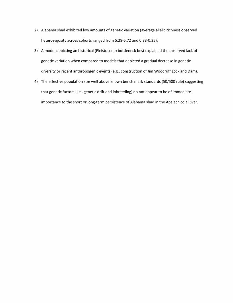
2) Alabama shad exhibited low amounts of genetic variation (average allelic richness observed

heterozygosity across cohorts ranged from 5.28-5.72 and 0.33-0.35).

3) A model depicting an historical (Pleistocene) bottleneck best explained the observed lack of

genetic variation when compared to models that depicted a gradual decrease in genetic

diversity or recent anthropogenic events (e.g., construction of Jim Woodruff Lock and Dam).

4) The effective population size well above known bench mark standards (50/500 rule) suggesting

that genetic factors (i.e., genetic drift and inbreeding) do not appear to be of immediate

importance to the short or long-term persistence of Alabama shad in the Apalachicola River.

Introduction

Some of the greatest estimates of aquatic species diversity in North America are found in the

freshwater systems of the southeastern United States (Lydeard and Mayden 1995, Neves et al 1997,

Crandal l and Buhay 2008). This rich aquatic fauna also has an alarming degree of imperilment (Jelks

Neves Williams). Perhaps one of the more notable river systems exhibiting this pattern of high species

diversity and imperilment is the Apalachicola Chattahoochee-Flint (ACF) River basin. Like many of the

freshwater systems of the Southeast, the ACF basins is experiencing human population growth and is

one of the most rapidly growing regions of the United States. As such, the ACF is heavily relied upon as

an important source and supply of water for human consumption, agriculture, and recreation (Barnett

2007) and has been highly publicized for the ongoing water allocation dispute between Alabama,

Georgia, and Florida. Habitat loss and fragmentation, which are leading causes of global reductions in

biodiversity (Brook et al., 2003; Fahrig, 2003), are often cited for declines in aquatic biodiversity of the

southeastern United States (Neves et al 1997, Warren et al 1997). Yet biodiversity and its loss are often

measured in terms of species diversity with little attention or understanding as to how these processes

affect other levels of biodiversity.

On such level of biodiversity, which is recognized by the World Conservation Union, is genetic

diversity (McNeely et al,1990). Genetic diversity is an important factor influencing population viability

and maintaining genetic diversity of populations (both within and between populations) is fundamental

for future adaptation to changing environmental conditions and other more immediate threats such as

disease, competition from invasive species and parasites (Brook et al., 2002). ). For example, as

populations become more and more fragmented, isolated sub-populations become the units on which

genetic drift, inbreeding, and selection act. Without the ameliorating influence of gene flow, their

concerted effects impose a more rapid erosion of genetic diversity, exacerbating fitness reductions and

extinction risks. In a climate of proposed management actions in the ACF basin to meet emerging water

needs (including changes in reservoir operation schedules and construction of new water supply

reservoirs) the estimation and monitoring of genetic diversity (both within and among populations)

should be a key consideration when developing conservation and management strategies for

threatened or endangered taxa of the ACF because it can provide for 1) an understanding of the present

and historical levels genetic diversity in a population or species (e.g., prior to release of hatchery

individuals), 2) an assessment of the alteration of these characteristics (i.e., perhaps due anthropogenic

factors), and 3) an evaluation of the biological consequences of management and conservation

initiatives (Schwartz et al. 2007; Laikre et al. 2010).

The goal of this study was to provide an initial assessment of genetic parameters to assess the

influence of genetic factors pertaining to extinction risk for two species of concern in the ACF – Alosa

alabamae (the Alabama shad) and Amblema neislerri (the fat threefridge). In doing so, we also provide

an initial assessment of genetic parameters for potential genetic monitoring of each species. We

accomplished our goal by 1) evaluating the extent of population substructure within ACF, 2) establishing

an estimate of genetic diversity (number of alleles and heterozygosity), 3) estimating Ne, and 4) testing

whether the observed genetic variation present in each species could be attributed anthropogenic or

more historic (Pleistocene) events.

The anadromous fish species Alosa alabamae occurs throughout the northern Gulf of Mexico.

Historically, this species ranged from the Suwannee River, FL, to the Mississippi River, LA and was known

to migrate inland as far as the Ohio and Missouri river drainages (Lee et al. 1980; Pattillo et al. 1997).

Once found in large numbers, this species in now considered rare or has been extirpated from many

rivers within its historical range. Such decline in distribution and abundance has prompted the National

Oceanic and Atmospheric Administration (NOAA) to list A. alabamae as a species of concern (Federal

Register 2004)(19975, Vol. 69, No. 73, 15 April 2004) due to lack of information available about the

species. Presently, the largest spawning population of A. alabamae occurs in the Apalachicola River, FL

(McBride 2000; Mettee and O’Neil 2003) below Jim Woodruff Lock and Dam and while the lock is an

impediment to upstream migration, migration has been documented upstream to the City Mills and

Eagle & Phenix Dams on the Chatahoochee River, and to the Albany Dam on the Flint River.

The life history of A. alabamae is similar to many salmonid species in that A. alabamae is

considered anadromous (Boschung and Mayden) and presumed to be phylopatric (i.e., its Atlantic coast

relative A. sapadisima exhibits phylopatry; Melvin et al. 1986; Hendricks et al. 2002). The spawning run

for the ACF population begins as early as February (Laurence 1967) when sexual mature males (ages 1-3)

and females (ages 2-4) migrate into freshwater (Ingram 2007). Spawning is thought to occur in swift

water over sandy substrate, gravel shoals, or limestone outcrops, (Shaeffer et al 2010). The ACF

population appears semelparous (Ingram 2007), but studies in the 1960-70s found that 25–57% of the

adult A. alabamae in the Apalachicola River, FL, were repeat spawners (Mills 1972, Laurence and Yerger

1967). Larvae develop into juveniles in freshwater and then migrate to estuaries in late fall or winter

(Bakuloo et al 1995).

The freshwater mussel, A. neislerii, is an endangered endemic whose historical distribution once

spanned 308 river miles of the ACF. Currently it is only found in 42 percent of its historical range that

includes the Apalachicola, Chipola (tributary of the Apalachicola River), and lower Flint rivers (Brim-Box

et al. 2000; USFWS, unpubl. data 2006). Like all freshwater mussels, A. neislerii requires a host fish to

complete its life cycle. Fertilization of freshwater mussels takes place in the suprabranchial chamber of

the female mussel (Jirka and Neves 1992). The fertilized eggs remain in the marsupial gills until they

develop into a parasitic stage called glochidia (Lefevre and Curtis 1912, Coker 1919). When fully

developed, the glochidia are released from the female mussels into the water column where they must

come into contact with a proper host fish. Once attached to the host fish, the glochidia become

encysted, metamorphose, and drop to the substrate to become juveniles. Glochidia failing to come into

contact with a suitable host will drift through the water column, surviving for only a few days (Jansen

1990).

There is little published literature pertaining to the life history of A. neislerii. Based on findings

from a closely-related congener A. plicata, Amblema neisleri is presumed to reach sexual maturity at

three years of age (Haag and Stanton 2003) for both males and females and are long-lived reaching a

maximum age of approximately 24 years of age (G. Moyer USFWS pers com.).

Historical records for anadromous species in the Chattahoochee and Flint Rivers are limited by

the past construction of dams as well as incomplete survey data. Dam construction in the

Chattahoochee River Basin began in the early 1800s at Columbus, GA, with the construction of City Mills

Dam and Eagle & Phenix Dam in the area of the Fall Line. Because the lower dam (Eagle & Phenix) is

impassable to Alabama shad, and because these dams are located at the Fall Line, there has been no

access above the Fall Line for Alabama shad since the dams were completed. Therefore, historical

records for Alabama shad in the upper Chattahoochee are limited since reports would have occurred

prior to dam construction. Anadromous spawning migrations upstream to the Fall Line (Eagle & Phenix

tailrace) were additionally impacted by the construction of three USACE lock and dams (Jim Woodruff,

George W. Andrews, and Walter F. George) that were completed in the 1950s and 1960s. In the

mainstem Flint River, two dams were constructed below the Fall Line in the 1920s that similarly

prevented spawning migrations to the upper reaches of this stream.

As noted, these deterministic events can adversely impact a population by decreasing

population size and by increasing the number of smaller populations (Thomas,2000; Fahrig, 2003).

However, small populations are often vulnerable to random fluctuations in demographic,

environmental, and genetic processes -- all of which are not mutually exclusive and can influence the

rate of extinction (Gilpin and Soule 1986; Reed 2010). ). For example, as populations become more and

more fragmented, each isolated sub-populations become the units on which genetic drift, inbreeding

and selection act. Without the ameliorating influence of gene flow, their concerted effects impose a

more rapid erosion of genetic diversity, exacerbating fitness reductions and extinction risks.

In a climate of proposed management actions in the ACF basin to meet emerging water needs (including

changes in reservoir operation schedules or construction of new water supply reservoirs) and contains.

substantial evidence suggests that genetic diversity is indeed an important factor influencing

population viability and is. Maintaining the genetic diversity of populations

which is regconized which sthe influence major divers of biodiversity loss are influenceWhile

aquatic biodiversity and its loss is often measured in terms of species diversity, the IUCN,the World

conservation Union, recognizes the need to conserve biodiversity at three levels: genetic, species, and

ecosystem diversity Yet biodiversity As noted, these deterministic events can adversely impact a

population by decreasing population size and by increasing the number of smaller populations

(Thomas,2000; Fahrig, 2003). However, small populations are often vulnerable to random fluctuations

in demographic, environmental, and genetic processes -- all of which are not mutually exclusive and can

influence the rate of extinction (Gilpin and Soule 1986; Reed 2010). ). For example, as populations

become more and more fragmented, each isolated sub-populations become the units on which genetic

drift, inbreeding and selection act. Without the ameliorating influence of gene flow, their concerted

effects impose a more rapid erosion of genetic diversity, exacerbating fitness reductions and extinction

risks.

In a climate of proposed management actions in the ACF basin to meet emerging water needs (including

changes in reservoir operation schedules or construction of new water supply reservoirs) and contains.

The southeastern region encompassing the Apalachicola Chattahoochee-Flint (ACF) River basin

is one of the most rapidly growing regions of the United States. The ACF is heavily relied upon as an

important source of water supply both for human consumption, agriculture, and recreation (Barnett

2007) and has been highly publicized for the ongoing water allocation dispute between Alabama,

Georgia, and Florida. The basin also supports one of the most diverse assemblages of freshwater

mussels in the southeast along with numerous aquatic species of conservation concern. Two such

species of concern are the fat threeridge (Amblema neislerii) and the Alabama shad (Alosa alabamae).

As noted, these deterministic events can adversely impact a population by decreasing

population size and by increasing the number of smaller populations (Thomas,2000; Fahrig, 2003).

However, small populations are often vulnerable to random fluctuations in demographic,

environmental, and genetic processes -- all of which are not mutually exclusive and can influence the

rate of extinction (Gilpin and Soule 1986; Reed 2010). ). For example, as populations become more and

more fragmented, each isolated sub-populations become the units on which genetic drift, inbreeding

and selection act. Without the ameliorating influence of gene flow, their concerted effects impose a

more rapid erosion of genetic diversity, exacerbating fitness reductions and extinction risks.

In a climate of proposed management actions in the ACF basin to meet emerging water needs (including

changes in reservoir operation schedules or construction of new water supply reservoirs) and contains.

The importance of genetic variation as a basis for future biological evolution and long term

viability of populations, species, and ecosystems is well establish (Frankel and Soule 1981, Frankham

2005, Laikre et al 2010), and its importance is reflected by the International Union for Conservation and

Nature’s recognition that genetic diversity is an essential component of biodiversity (McNeely et al.

1990). Unforturnately, the recognition of conservation genetic concerns in practical management is

largely lacking (Laikre 2010).

I For example, substantial evidence suggests that genetic diversity is indeed an important factor

influencing population viability and is therefore a key consideration when developing conservation and

management strategies for threatened taxa. Maintaining the genetic diversity of populations is

fundamental for future adaptation to changing environmental conditions and other more immediate

threats such as disease, competition from invasive species and parasites (Brook et al., 2002).

by increasing population isolation and thus reducing gene flow and by increasing inbreeding and thus

reducing population fitness (Nieminen et al., 2001; Keller &Waller, 2002). Therefore, many populations

of aquatic species in the southeast must also be experience a depletion of genetic diversity due to

incresaded genetic drift and inbreeding.

Major drivers of habitat loss, fragmentation and degradation have been linked to water impoundments

(e.g as physical barriers to gene flow and physical alteration of habitat and changes to flow regimes).

and is often identified as a reion with high biodiversity that is subjected to rapid environmental

changes.

of the species given endanger or threaten status by the United States Fish and Wildlife Service. Even

more alarming is that this percentage has increased through time with greater ()

Beyond two historic descriptive studies conducted on the Apalachicola River (Laurence and

Yerger 1966, Mills 1972) no detailed data regarding population distribution and abundance, genetic

structure, and habitat requirements of Alabama shad are available. Recognizing the need for restorative

research and action, the Alabama Shad Restoration and Management Plan for the Apalachicola-

Chatahoochee-Flint (SCF) river basin was drafted and is a joint venture among Alabama Department of

Conservation and Natural Resources, Florida Fish and Wildlife Conservation Commission, Georgia

Department of natural Resources, National Marine Fisheries Service, South Carolina Cooperative Fish

and Wildlife Research Unit, The Nature Conservancy, and the United States Fish and Wildlife Service.

Among other objectives, the management plan sought to examine the genetic diversity and calculate

the effective population size of the existing wild Alabama shad population.

Genetic variation is important in maintaining the adaptive potential of species/populations and

the fitness of individuals to help ensure their survival (Frankel and Soule 1981, Frankham 2005, Laikre et

al 2010): its importance is reflected by the International Union for Conservation and Nature’s

recognition that genetic diversity is an essential component of biodiversity (McNeely et al 1990).

Monitoring temporal fluctuations in population genetic metrics or other population data generated

using molecular markers is an integral tool for the conservation of threatened or endangered species

because it can provide for 1) an understanding of the present and historical levels genetic diversity in a

population or species (e.g., prior to release of hatchery individuals), 2) an assessment of the alteration of

these characteristics (i.e., perhaps due anthropogenic factors), and 3) an evaluation of the biological

consequences of management and conservation initiatives (Schwartz et al. 2007; Laikre et al. 2010).

Parameters most often used in population genetic monitoring include allelic richness (number of alleles

per locus), allelic evenness (heterozygosity), and effective population size; Schwartz et al 2007,

Aravanopoulos 2010).

The goal of this study was to provide an initial assessment of genetic parameters to assess the

influence of genetic factors pertaining to extinction risk for Alabama shad in the Apalachicola River. In

doing so, we also provide an initial assessment of genetic parameters for potential genetic monitoring of

this species. We accomplished our goal by 1) evaluating the extent of population substructure within

ACF, 2) establishing an estimate of genetic diversity (number of alleles and heterozygosity), 3) estimating

Ne, and 4) testing whether the observed genetic variation present Alabama shad could be attributed

anthropogenic or more historic events.

Materials and Methods

Clemson University and Georgia Department of Natural Resources provided fin clips from

Alabama shad collected in 2005 (n = 100), 2008 (n = 144), 2009 (n = 97), 2010 (n = 192), and 2011 (n =

96). Fish were collected from May-March (representing the spawning run) in Apalachicola River, Florida,

2 km downstream of Jim Woodruff Lock and Dam (JWLD) via boat electrofishing or angling. Jim

Woodruff Lock and Dam is located at river km 172 on the Apalachicola River and represents the first

barrier to migration for anadromous fish. Positioned at the confluence of the Flint and Chattahoochee

rivers, JWLD forms Lake Seminole and is used for hydroelectric power and locking from the Apalachicola

River to Lake Seminole. Our sampling location was chosen because migrating adult Alabama shad

impeded by the dam congregate in this area. DNA was extracted from a proportion of the ethanol

preserved fin clip using the DNeasy® Blood and Tissue kit (QIAGEN, Inc., Valencia, California) protocol.

We used multiplex polymerase chain reactions (PCR) on a suite of 11 microsatellite markers

known to amplify in American shad (Julian and Bartron 2007). Multiplex PCR amplifications were

performed in 20 μL reactions using the following reaction components: 1 × Taq reaction buffer (Applied

Biosystems Inc., Foster City, California), 3.75 mM MgCl2, 0.423 mM of each dNTP, 0.25 μM of each

primer, and 0.08 U Taq polymerase (Applied Biosystems, Inc.). PCR conditions were an initial

denaturation at 94 °C (10 min), followed by a touchdown procedure involving 33 cycles and consisting of

denaturing (94 °C, 30 s), annealing, and extension (74 °C, 30 s) cycles, where the initial annealing

temperature was initiated at 56 ºC and decreased by 0.2 °C per cycle for 30 s. Prior to electrophoresis, 2

μL of a 1:100 dilution of PCR product was mixed with a 8 μL solution containing 97% formamide and 3%

Genescan™ LIZ® 500 size standard (Applied Biosystems, Inc.). Microsatellite reactions were visualized

with an ABI 3130 genetic analyzer (Applied Biosystems, Inc.) using fluorescently labeled forward primers

and analyzed using GeneMapper® software v3.7 (Applied Biosystems, Inc.).

Genetic diversity, in the form of average number of alleles, observed heterozygosity, and

expected heterozygosity, was calculated for each cohort of Alabama shad in the Apalachicola River using

the computer program GenAIEx (Peakall and Smouse 2006). HP-RARE (Kalinowski 2005) was used to

estimate allelic richness (note that allelic richness in an estimate of number of alleles that is corrected

for sample size). Tests for significance among cohorts were conducted using the Wilcoxon rank-sum test

(Sokal and Rohlf 1995) as implemented in S-Plus v7.0 (Insightful Corporation).

To assess stock structure, we tested the hypothesis that the collected samples were of one large

panmictic population (we could not use a molecular variation approach outlined in the proposal because

all individuals came from the same approximate sampling location). Our expectation is that each cohort

should be in Hardy–Weinberg equilibrium and gametic disequilibrium if no stock structure is present.

Gametic disequilibrium tests (all pairs of loci per cohort) and locus conformance to HWE (for each locus

in a cohort) were implemented using GENEPOP v4.0.10 (Raymond and Rousset 1995). Significance

levels for all simultaneous tests were adjusted using a sequential Bonferroni correction (Rice 1989).

We also assessed the degree of population structure in Alabama shad by using a Bayesian-based

clustering algorithm implemented in the program STRUCTURE v2.3.3 (Pritchard et al. 2000; Falush et al.

2003). STRUCTURE assumed no a priori sampling information; rather, individuals were assigned to

groups in such a way as to achieve Hardy-Weinberg and gametic equilibriums. STRUCTURE was run with

three independent replicates for K (i.e., distinct populations or gene pools), with K set from one to four.

The burn-in period was 20,000 replicates followed by 100,000 Monte Carlo simulations (number of

iterations was set to three) run under a model that assumed no admixture and independent allele

frequencies. The mean and standard deviation of likelihood estimates (Pr[X/K] = posterior probability of

the data given K populations) among runs at each values of K and estimates of delta K (Evanno et al.

2005) were used to determine the most likely value of K.

Estimation of effective population sized (Ne) was assessed by estimating temporal changes in

allele frequencies (F�) among cohorts (Nei and Tajima 1981); however, the presumed semelparity of

Alabama shad (Ingram 2007) allowed us to use a modified method outlined by previous studies (Waples

1989; 1990). Waples (1989, 1990) showed that the rate of change of neutral allele frequency in a

semelparous Pacific salmon population with Nb effective breeders each year was the same as in an

organism with discrete generations and effective population size = gNb , were g is the generation length.

Since adults were sampled nondestructively before spawning (equivalent to sampling plan I in the

discrete generation model; Nei and Tajima 1981), we estimated Nb using the equation

N�b= b/(2(F�-1/S�+1/N)

(Waples 1990) where b is the slope of the regression of 2S�F� on S�/Nb (Waples 1990), S� is the harmonic

mean of the number of individuals sampled, and N is total number of spawners subject to the sampling

process. We estimated b and g by solving a set of linear equations given information about the number

of spawners returning at each year class (Tajima 1992). Estimation of number of spawners for each age

class 1-4 was 0.33, 0.39, 0.26, and 0.02, respectively (Ingram 2007). Population size for each yearly

sample of Alabama shad reaching JWLD was estimated by mark – recapture via the Schnabel multiple

census method (Ricker 1975). Per cohort population size was then summed and used for a value of N in

the estimation of Nb. The parameter F� was estimated for all pairwise comparisons among sampling

years (ten comparisons). These values were averaged to produce and overall estimate of F�. The

confidence interval (CI) for F� was computed from the formula

95% CI for F� = �nF�

χ0.025 [n]2 ,

nF�χ0.9755 [n]

2 �

Waples (1989), where χ0.025 [n]2 is the critical chi-square valued for n degrees of freedom and α/2 = 0.025

(Sokal and Rohlf 1995). The 95% confidence interval for F� computed as above was based on using n =

675 degrees of freedom (10 - 1 = 9 degrees of freedom for each of the 76 - 1 independent alleles). Once

N�b was obtained, we estimated Ne (N�e) as gN�b. Confidence in this estimate was obtained by using the

95% CI for F�, which provided a 95% CI for N�b and subsequently for N�e.

We tested whether the lack of genetic diversity in Alabama shad (see below) was attributed to a

recent or a more historical bottleneck by testing competing hypothesis in an approximate Bayesian

computation (ABC) framework (Beaumont et al. 2002), as implemented by the program DIY ABC

v1.0.1.34beta (Cornuet et al. 2008). This approach was employed to model evolutionary scenarios given

a uniform distribution of values for each parameter (discussed below) and summary statistics based on

the observed microsatellite data. Summary statistics included average number of alleles, expected

heterozygosity, allele size variance across loci, and M-index (Garza and Williamson 2001). The ABC

method entailed generating simulated data sets (based on the microsatellite data), selecting simulated

data sets closest to observed data set, and estimating posterior distributions of parameters through a

local linear regression procedure (Beaumont et al. 2002; Cornuet et al. 2008). In doing so, this approach

provided a way to quantitatively compare alternative evolutionary scenarios.

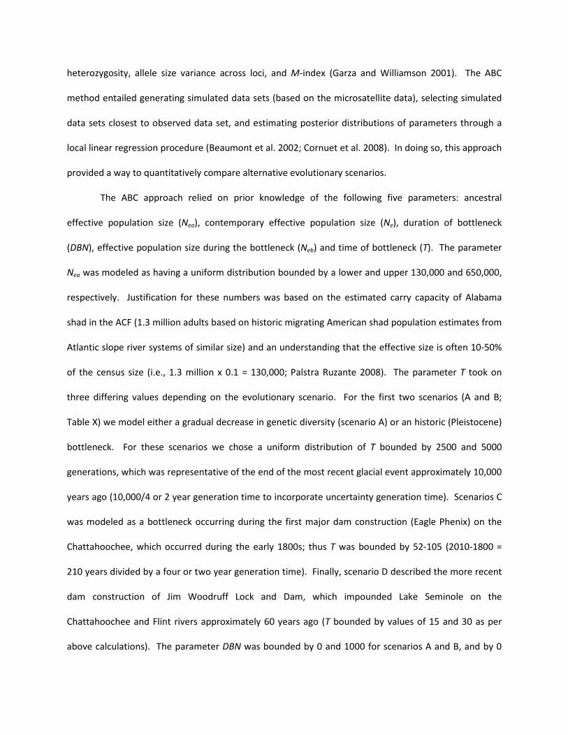
The ABC approach relied on prior knowledge of the following five parameters: ancestral

effective population size (Nea), contemporary effective population size (Ne), duration of bottleneck

(DBN), effective population size during the bottleneck (Neb) and time of bottleneck (T). The parameter

Nea was modeled as having a uniform distribution bounded by a lower and upper 130,000 and 650,000,

respectively. Justification for these numbers was based on the estimated carry capacity of Alabama

shad in the ACF (1.3 million adults based on historic migrating American shad population estimates from

Atlantic slope river systems of similar size) and an understanding that the effective size is often 10-50%

of the census size (i.e., 1.3 million x 0.1 = 130,000; Palstra Ruzante 2008). The parameter T took on

three differing values depending on the evolutionary scenario. For the first two scenarios (A and B;

Table X) we model either a gradual decrease in genetic diversity (scenario A) or an historic (Pleistocene)

bottleneck. For these scenarios we chose a uniform distribution of T bounded by 2500 and 5000

generations, which was representative of the end of the most recent glacial event approximately 10,000

years ago (10,000/4 or 2 year generation time to incorporate uncertainty generation time). Scenarios C

was modeled as a bottleneck occurring during the first major dam construction (Eagle Phenix) on the

Chattahoochee, which occurred during the early 1800s; thus T was bounded by 52-105 (2010-1800 =

210 years divided by a four or two year generation time). Finally, scenario D described the more recent

dam construction of Jim Woodruff Lock and Dam, which impounded Lake Seminole on the

Chattahoochee and Flint rivers approximately 60 years ago (T bounded by values of 15 and 30 as per

above calculations). The parameter DBN was bounded by 0 and 1000 for scenarios A and B, and by 0

and 12 (duration of dam construction) for scenarios C and D. During this duration Neb was assumed to

be between a value of 2 and 500. Finally, the lower and upper bounds (1184 and 47500) for our

distribution of Ne were conservative and estimated as 50% of the lower and upper spawning abundance

estimates (2,368 and 98,000; see below).

We simulated 1,000,000 datasets per scenario (via DIY ABC) to produce reference datasets using

uniform priors for each parameter (Table 3). Prior information regarding the mutation rate and model

for microsatellites was taken as the default values in DIY ABC. The posterior distribution of each

scenario was estimated using local linear regression on logit transformed data for the 10,000 simulated

datasets closest to the observed dataset (Cornuet et al. 2008). The exact posterior probability of each

scenario was reliant on the model that generated the posterior probability distribution; therefore, poor

model fit could lead to inaccurate estimation of the models posterior distribution and subsequent model

choice (Cornuet et al. 2010). As recommended by Cornuet et al. (2010), we employed the model

checking function of DIY ABC to assess the goodness-of-fit between each model parameter posterior

combination and the observed dataset by using different summary statistics for parameter estimation

and model discrimination. The parameter estimation summary statistics used were M-index and allele

size variance, while the model discrimination summary statistics were average number of alleles and

average expected heterozygosity. Finally, we evaluated the level of confidence in the choice of the best

supported scenario by estimating type I and II errors. We simulated 450 data sets using the scenario

with the highest posterior probability to estimate parameters to which all other scenarios were

compared. Then we counted the proportion of times that the scenario with the highest posterior

probability did not generate the highest posterior probability among the three competing scenarios

when it was the true scenario (type I error) or the proportion of times that the scenario had the highest

posterior probability when it was not the true scenario (type II error, estimated from test data sets

simulated under the other competing scenarios).

Results

A total of 628 Alabama shad were analyzed using 11 microsatellite markers. Average number of

alleles and observed heterozygosity were similar for each sample year and ranged from 5.45-6.00 and

0.33- 0.35, respectively (Table 1). The number of alleles, observed heterozygosity, and expected

heterozygosity were not significantly different among cohorts (all P > 0.74). For each year, all loci

conformed to per locus HWE (all P > 0.12) except for locus D429, which showed a significant (p <0.001)

excess of homozygotes in years 2005 and 2008. Microchecker indicated that the significance may be

due to null alleles as indicated by the general excess of homozygotes at most allele size classes. This

locus was removed from all subsequent analyses. All loci showed gametic equilibrium after sequential

Bonferroni correction (all P > 0.01, n = 48 comparisons, α = 0.001 after Bonferroni correction).

STRUCTURE analysis revealed K = 2 using the Evanno et al. (2005) method (Figure 1); however, the

proportion of sampled individuals to each sampling site was symmetrical for all K-values 2-4, which is an

indication of no population structure (Pritchard et al. 2000; Evanno et al. 2005).

Pairwise estimates of F�, for each sample year (Table 2; see Appendix for allele frequency data)

ranged from 0.0050-0.0110 and averaged 0.0078 (95% CI = 0.0070-0.0087). The harmonic mean of per

cohort samples sizes (S�) was 116, and b and g were estimated to be 1.67 and 1.97, respectively.

Estimation of the number of spawners for 2005, 2008, 2009, 2010, and 2011 was 25·935, 2·368, 10·753,

98·469, and 26·193. respectively. Summing individual estimates of population size yielded a value for N

of 163·718. Using values of b, F�, S� and N, we obtained a value for N�b -1·040 (95% CI = 8·166-∞) and an

estimate for N�e= gN�bof -2·048 (95% CI = 16·087-∞). Note that a value negativ implies our data provided

no evidence that the population is not very large (Nei and Tajima 1981; Waples and Do 2010).

We were interested in testing whether the observed genetic variation present Alabama shad

could be attributed anthropogenic events (e.g., the construction of Jim Woodruff Lock and Dam);

therefore, we tested four alternative evolutionary scenarios that might explain the observed genetic

variation. Scenario B, which was the model depicting a past Pleistocene bottleneck, produced a

posterior probability of 0.9025 (95% confidence interval of 0.8971 - 0.9079; Table 3) suggesting that this

scenario explained the observed data better than competing hypotheses. Scenario B was also the only

scenario for which none of the test quantities used to assess model misfit had low tail probability values

(Table 3) indicating a good fit of the scenario-posterior combination to the pseudo-observed data set.

Over the 450 data sets simulated using scenario B, 84% exhibited scenario B as having the greatest

posterior probability when compared to competing scenario C; thus, our estimate of type I error was

16%. In contrast, only 6% of the data sets had the largest posterior probability for scenario B when data

sets were created using scenario C indicating that type II error was minimized.

Discussion

Fish population genetic structure is often associated with barriers to gene flow and typically

coincides with differences among major river basins. However, anadromous fish such as salmon species

typically migrate to their natal river to spawn and often demonstrate fine-scale structure in a river or

river system. Like salmon, Alabama shad migrate to their natal river to spawn (Ingram 2007 and

references there in); therefore, unrecognized population structure within the ACF river system could

exist. Our data provided no evidence of fine-scale population structure in the ACF. Microsatellite

markers were in accordance with HWE and gametic equilibrium and while Bayesian cluster analysis

revealed the potential for two distinct groups, the proportion of sampled individuals to each sampling

site was symmetrical for all K values, which is an indication of no population structure (Pritchard et al.

2000; Evanno et al. 2005). Our findings were consistent with previous genetic studies (Hasselman 2010,

and references there in) that concluded American shad spawning site fidelity appeared nonexistent at

fine spatial scales.

The observed genetic variation (both number of alleles and observed heterozygosity) found in

Alabama shad was lower than expected based on other shad studies. Estimates of allelic richness and

observed heterozygosity, which range from 7-11 and 0.68-0.80 for spawning populations of American

shad distributed along the Atlantic coast (Hasselman 2010), were in stark contrast to estimates found in

Alabama shad (5-6 and 0.33- 0.35). These findings suggest that the genetic variation of Alabama shad in

the Apalachicola River has been severely impacted by some type of bottleneck event. We found no

evidence indicating that this bottleneck was anthropogenic in origin; rather it appears the result of past

events presumably during the Pleistocene.

Data pertaining to past and present processing that have shaped present levels of genetic

variation are critical to management and conservation because information gleaned from conservation

genetics can assist in the proper design, implementation, and monitoring of management and

conservation strategies of imperiled species. For example, populations or species that have undergone

population bottlenecks throughout their evolutionary history may have reduced genetic load (genetic

defined as the reduction in mean fitness resulting from detrimental variation for a population when

compared to a population without lowered fitness) and thus be less prone to have inbreeding

depression during population bottlenecks. As a consequence, such a population may have increased

viability and be more likely to recover from near-extinction/extirpation than population lacking such a

history (Hedrick 2001). This type of a scenario may be the case for Alabama shad. Simulations using an

ABC approach indicated that the bottleneck was both intense (Ne during the bottleneck was estimated

to be between 76 and 398) and prolonged (duration of bottleneck was approximately 145-987

generations). The bottleneck, therefore, may have purged much of their genetic load making the

population less prone to have fitness deceases in the event that another bottleneck should arise. While

the risk of inbreeding depression appears low, the efficiency of purging is difficult to predict because

bottlenecks may have variable outcomes regarding their effects on genetic diversity, fitness, and

extinction (Bouzat 2010). Therefore, Apalachicola River Alabama shad should be monitored for and

protected from any depression of demographic rate that could cause the population to decline.

Likewise, if hatchery augmentation is every implemented for this species, inbreeding should be avoided

as much as possible in order to minimize inbreeding depression. This entails establishing a clear

conservation hatchery plan that minimized mean kinship between parents (Ballou and Lacy 1995) and

maximizes Ne (Allendorf 1993).

The cause of the bottleneck is unknown, but based on the estimated value of T for scenario B, it

occurred approximately 3620 generations ago (95% CI of 2540 - 4920) and corresponds roughly to the

early Holocene (assuming that Alabama shad had a two year generation time). This time period

corresponded with the last lowstand of sea level where rivers such as the Apalachicola drained to the

outer continental shelf. Thus low water levels and or the establishment of a continuous offshore shoal

(Osterman et al 2009) could have restricted the influx of American shad in to the Apalachicola River.

Conversely, intensive exploitation of marine shellfish and fish has been documented as early as 4000–

5000 years ago in this region (Saunders and Russo 2009).

While the genetic diversity was low for Alabama shad in the Apalachicola River, the risk of losing

genetic diversity appeared minimal due to the rather large estimate of Ne. The effective population size

can be used to predict the expected rate of loss of genetic variation (in terms of heterozygosity). That is

to say, the smaller the effective size the greater the rate of loss of genetic variation. Our estimate of Ne

was infinite but had a lower bound of 16,087. If this is compared to known bench marks such as the

50/500 rule (Franklin 1980), where as a general rule of thumb, in the short term Ne should not be less

than 50 and in the long term should not be less than 500, then our estimate of Ne was well above these

thresholds and suggests that genetic factors (i.e., genetic drift and inbreeding) do not appear to be of

immediate importance to the short or long-term persistence of Alabama shad in the Apalachicola River

(given the assumption that biotic and abiotic factors remain relatively stable over time).

Perhaps the main consequence of reduced variability is the presumption that loss of genetic

diversity can reduce an organism’s adaptive capacity to respond to differing environmental conditions

and thereby increasing extinction risk. For example, when for populations of Drosophila of variously

inbred and outbred lines were exposed to increasing salt concentrations, the relatively outbred

populations proved better able to adapt over time (Frankham et al 1999). Unfortunately, it is often

difficult to maintain and predict an organism's adaptive genetic potential, but genomic approaches may

one day allow the identification of adaptive genetic variation related to key traits such as phenology

(Allendorf et al 2010).

In conclusion, the importance of genetic variation, as a basis for future biological evolution and

long-term viability of populations, species, and ecosystems, are well established (Frankel and Soule

1981; Frankham 1995). Therefore, identifying and monitoring processes that are likely to have adverse

impacts on the conservation of natural populations are becoming increasingly important.

Unfortunately, most conservation programs do not take full advantage of the potential afforded by

molecular genetic markers (Schwartz et al. 2007; Laikre 2010). Genetic data collected in this study serve

as a reference for comparison in an ongoing effort to monitor temporal changes in population genetic

metrics as well as assess and predict potential extinction risks associated with genetic stochasticity. The

risk of population decline and extinction due to inbreeding depression and genetic drift appears low;

however, the limited amount of genetic diversity may inhibit the ability for this organism to respond to

unanticipated environmental and anthropogenic changes – a risk that is difficult to prioritize given the

available genetic data. These data will provide guidance and a means to evaluate the effectiveness

(both in terms of increasing the census size and maintaining the long-term viability of the population)

for hatchery augmentation if the need should ever arise.

Literature Cited

Allendorf, F. W. 1993. Delay of adaptation to captive breeding by equalizing family size. Conservation

Biology 7:416-419.

Allendorf, F. W., P. A. Hohenlohe, and G. Luikart. 2010. Genomics and the future of conservation

genetics. Nat Rev Genet 11:697-709.

Aravanopoulos, F. A. 2011. Genetic monitoring in natural perennial plant populations. Botany 89:75-81.

Ballou, J., and R. C. Lacy. 1995. Identifying genetically important individuals for management of genetic

variation in pedigreed populations. Pages 76-111 in J. D. Ballou, editor. In Population

Management for Survival and Recovery. Columbia University Press.

Beaumont, M. A., W. Zhang, and D. J. Balding. 2002. Approximate Bayesian computation in population

genetics. Genetics 162:2025-2035.

Bouzat, J. 2010. Conservation genetics of population bottlenecks: the role of chance, selection, and

history. Conservation Genetics 11:463-478.

Cornuet, J.-M., V. Ravigne, and A. Estoup. 2010. Inference on population history and model checking

using DNA sequence and microsatellite data with the software DIYABC (v1.0). BMC

Bioinformatics 11:401.

Cornuet, J.-M., F. Santos, M. A. Beaumont, C. P. Robert, J.-M. Marin, D. J. Balding, T. Guillemaud, and A.

Estoup. 2008. Inferring population history with DIY ABC: a user-friendly approach to

approximate Bayesian computation. Bioinformatics 24:2713-2719.

Ely, P. C., S. P. Young, and J. J. Isely. 2008. Population size and relative abundance of adult Alabama shad

reaching Jim Woodruff Lock and Dam, Apalachicola River, Florida. North American Journal of

Fisheries Management 28:827-831.

Evanno, G., S. Regnaut, and J. Goudet. 2005. Detecting the number of clusters of individuals using the

software STRUCTURE: a simulation study. Molecular Ecology Notes 14:2611-2620.

Falush, D., M. Stephens, and J. K. Pritchard. 2003. Inference of population structure using multilocus

genotype data: Linked loci and correlated allele frequencies. Genetics 164:1567-1587.

Frankel, O. H., and M. E. Soule. 1981. Conservation and Evolution. Cambridge University Press,

Cambridge, UK.

Frankham, R. 1995. Conservation genetics. Annual Review of Genetics 29:305-27.

Frankham, R. 2005. Conservation biology: ecosystem recovery enhanced by genotypic diversity. Heredity

95:183.

Frankham, R. 2010. Challenges and opportunities of genetic approaches to biological conservation.

Biological Conservation 143:1919-1927.

Frankham, R., K. Lees, M. E. Montgomery, P. R. England, E. H. Lowe, and D. A. Briscoe. 1999. Do

population size bottlenecks reduce evolutionary potential? Animal Conservation 2:255-260.

Franklin, I. R. 1980. Evolutionary changes in small populations. Pages 135-149 in M. E. Soule, and B. A.

Wilcox, editors. Conservation Biology, An Evolutionary-Ecological Perspective. Sinauer Assoc,

Sunderland.

Garza, J. C., and E. G. Williamson. 2001. Detection of reduction in population size using data from

microsatellite loci. Molecular Ecology 10:305-318.

Glémin, S. 2003. How are deleterious mutations purged? Drift versus nonrandom mating. Evolution

57:2678-2687.

Hasselman, D. J. 2010. Spatial distribution of neutral genetic variation in a wide ranging anadromous

clupeid, American shad (Alosa sapidissima). Doctor of Philosophy. Dalhousie University, Halifax.

Hasselman, D. J., R. G. Bradford, and P. Bentzen. 2010. Taking stock: defining populations of American

shad (Alosa sapidissima) in Canada using neutral genetic markers. Canadian Journal of Fisheries

and Aquatic Sciences 67:1021-1039.

Hedrick, P. W. 1994. Purging inbreeding depression and the probability of extinction: full-sib mating.

Heredity 73:363-372.

Hedrick, P. W. 2001. Conservation genetics: where are we now? Trends in Ecology & Evolution 16:629-

636.

Ingram, T. R. 2007. Age, growth and fecundity of Alablama shad (Alosa alabamae) in the Apalachicola

River, Florida. Master of Science. Clemson University, Clemson.

Julian, S., and M. Bartron. 2007. Microsatellite DNA markers for American shad (Alosa sapidissima) and

cross-species amplification within the family Clupeidae. Molecular Ecology Notes 7:805-807.

Kalinowski, S. T. 2005. HP-Rare: A computer program for performing rarefaction on measures of allelic

diversity. Molecular Ecology Notes 5:187-189.

Laikre, L. 2010. Genetic diversity is overlooked in international conservation policy implementation.

Conservation Genetics 11:349-354.

Laikre, L., M. K. Schwartz, R. S. Waples, and N. Ryman. 2010. Compromising genetic diversity in the wild:

unmonitored large-scale release of plants and animals. Trends in Ecology and Evolution 25:520-

529.

Laurence, G. C., and R. W. Yerger. 1966. Life history studies of the Alabama shad, Alosa alabamae, in the

Apalachicola River, Florida. Proceedings of the Annual Conference of the Southeastern

Association of Fish and Wildlife Agencies 20.

Lee, D. S., C. R. Gilbert, C. H. Hocutt, R. E. Jenkins, D. E. McAllister, and J. R. Stauffer. 1980. Atlas of North

American freshwater fishes, North Carolina State Museum of Natural History.

McNeely, J., K. Miller, W. Reid, R. Mittermeier, and T. Werner. 1990. Conserving the World's Biological

Diversity. IUCN, World Resources Institute, Conservation International, WWF-US and the World

Bank: Washington, DC.

Mettee, M. F., and P. O'Neil. 2003. Status of Alabama shad and skipjack herring in Gulf of Mexico

drainages. Pages 157-170 in K. E. Limburg, and J. R. Waldman, editors. Biodiversity, status, and

conservation of the world's shads. American Fisheries Society, Bethesda, MD.

Miller, L. M., and A. R. Kapuscinski. 2003. Genetic guidelines for hatchery supplementation programs.

Pages 329-355 in E. M. Hallerman, editor. Population genetics: principles and applications for

fisheries scientists. American Fisheries Society, Maryland.

Mills, J. G. 1972. Biology of the Alabama shad in northwest Florida. Florida Department of Natural

Resources Marine Research Laboratory Technical Series 68:1-24.

Moyer, G. R., and A. S. Williams. 2011. Assessment of genetic diversity for American shad in the Santee-

Cooper basin of South Carolina prior to hatchery augmentation. Marine Coastal Fisheries In

press.

Nei, M., and F. Tajima. 1981. Genetic drift and estimation of effective population size. Genetics 98:625-

640.

NOAA. 2004. Endangered and threatened species; establishment of species of concern list, addition of

species to species of concern list, description of factors for identifying species of concern, and

revision of candidate species list under the Endangered Species Act. Federal Register 69:11975-

19979.

Osterman, L., D. Twichell, and R. Poore. 2009. Holocene evolution of Apalachicola Bay, Florida. Geo-

Marine Letters 29:395-404.

Palstra, F. P., and D. E. Ruzzante. 2008. Genetic estimates of contemporary effective population size:

what can they tell us about the importance of genetic stochasticity for wild population

persistence? Molecular Ecology 17:3428-3447.

Peakall, R., and P. E. Smouse. 2006. GENALEX 6: genetic analysis in Excel. Population genetic software for

teaching and research. Molecular Ecology Notes 6:288-295.

Pritchard, J. K., M. Stephens, and P. Donnelly. 2000. Inference of population structure using multilocus

genotype data. Genetics 155:945-959.

Raymond, M., and F. Rousset. 1995. GENEPOP (version 1.2): population genetics software for exact tests

and ecumenicism. Journal of Heredity 86:248-249.

Reed, D. H., and R. Frankham. 2003. Correlation between fitness and genetic diversity. Conservation

Biology 17:230-237.

Rice, W. R. 1989. Analyzing tables of statistical tests. Evolution 43:223–225.

Saunders, R., and M. Russo. 2009. Coastal shell middens in Florida: A view from the Archaic period.

Quaternary International 239:38-50.

Schwartz, M. K., G. Luikart, and R. S. Waples. 2007. Genetic monitoring as a promising tool for

conservation and management. Trends in Ecology & Evolution 22:25-33.

Sokal, R. R., and F. J. Rohlf. 1995. Biometry: the principles and practice of statistics in biological research,

3 edition. W.H. Freeman and Company, New York.

Stapley, J., J. Reger, P. G. D. Feulner, C. Smadja, J. Galindo, R. Ekblom, C. Bennison, A. D. Ball, A. P.

Beckerman, and J. Slate. 2010. Adaptation genomics: the next generation. Trends in Ecology &

Evolution 25:705-712.

Tajima, F. 1992. Statistical method for estimating the effective population size in Pacific salmon. Journal

of Heredity 83:309-311.

Waples, R. S. 1989. A general approach for estimating effective population size from temporal changes

in allele frequency. Genetics 121:379-391.

Waples, R. S. 1990. Conservation genetics of pacific salmon. III. Estimating effective population size.

Journal of Heredity 81:277-289.

Waples, R. S., and C. Do. 2010. Linkage disequilibrium estimates of contemporary Ne using highly

polymorphic genetic markers: a largely untapped resource for applied conservation and

evolution. Evolutionary Applications 2010:244-262.

Table 1. Population genetic parameters for sampled Alabama shad in the Apalachicola River.

Abbreviations N, Na, Ho, and He represent the number of samples genotyped, average number of

alleles, observed heterozygosity and expected heterozygosity.

Year Locus N Na Ho He

2005 D21 100 5.000 0.270 0.266

D30 100 8.000 0.390 0.379

D31 100 2.000 0.010 0.010

D429 100 3.000 0.160 0.149

B20 100 3.000 0.190 0.190

D312 100 13.000 0.830 0.832

D55 100 3.000 0.250 0.241

C249 100 6.000 0.470 0.508

C334 100 5.000 0.490 0.475

D42 100 4.000 0.230 0.266

D392 100 9.000 0.650 0.576

Average

5.545 0.358 0.354

2008 D21 144 5.000 0.278 0.272

D30 144 8.000 0.403 0.384

D31 144 2.000 0.014 0.014

D429 144 3.000 0.090 0.112

B20 144 3.000 0.153 0.166

D312 143 18.000 0.818 0.811

D55 144 3.000 0.236 0.248

C249 143 6.000 0.510 0.523

C334 143 4.000 0.413 0.466

D42 143 4.000 0.203 0.198

D392 144 10.000 0.556 0.585

Average

6.000 0.334 0.343

2009 D21 97 5.000 0.309 0.340

D30 97 9.000 0.412 0.428

D31 97 1.000 0.000 0.000

D429 96 3.000 0.167 0.154

B20 97 3.000 0.206 0.197

D312 97 15.000 0.845 0.823

D55 97 3.000 0.247 0.256

C249 97 6.000 0.454 0.458

C334 97 3.000 0.485 0.469

D42 97 4.000 0.237 0.221

D392 96 8.000 0.521 0.590

Average

5.455 0.353 0.358

2010 D21 171 5.000 0.298 0.311

D30 186 8.000 0.349 0.382

D31 184 2.000 0.011 0.011

D429 184 2.000 0.136 0.154

B20 191 3.000 0.188 0.198

D312 191 16.000 0.838 0.812

D55 191 4.000 0.236 0.227

C249 175 6.000 0.526 0.523

C334 190 5.000 0.416 0.429

D42 190 5.000 0.200 0.192

D392 182 10.000 0.538 0.581

Average

6.000 0.340 0.347

2011 D21 93 4.000 0.280 0.288

D30 93 8.000 0.366 0.404

D31 94 2.000 0.011 0.011

D429 93 2.000 0.129 0.121

B20 93 3.000 0.194 0.184

D312 94 16.000 0.777 0.813

D55 94 4.000 0.287 0.273

C249 95 6.000 0.463 0.492

C334 95 4.000 0.516 0.474

D42 95 4.000 0.284 0.257

D392 92 8.000 0.533 0.514

Average

5.545 0.349 0.348

Table 2. Pairwise estimate of the temporal change in allele frequencies (F�) among Alabama shad

collection years.

2005 2008 2009 2010 2011

2005 -- 0.0080 0.0089 0.0107 0.0110

2008

-- 0.0063 0.0050 0.0073

2009

-- 0.0075 0.0051

2010

-- 0.0080

2011

--

Table 3. Prior uniform distributions, posterior probabilities, and summary statistics for coalescent models used to

compare competing evolutionary scenarios. Each scenario (A-D) was comprised of five parameters: ancestral

effective population size (Nea), effective population size during a bottleneck (Neb), duration of bottleneck (DBN, in

generations) contemporary effective population size (Ne ), and time of bottleneck (T). Each parameter was

sampled from a uniform distribution with lower and upper bounds indicated in brackets (refer to Material and

Methods for details about each uniform distribution). Also reported is the posterior probability for each

evolutionary scenario along with summary statistics (average number of alleles, No. alleles and expected

heterozygosity, He) used to assess the goodness-of-fit between each model parameter posterior combination and

the observed dataset. Test quantities (x), which corresponded to the summary statistics, were interpreted as the

probability (xsimulated < xobserved); therefore, values greater than 0.95 and less than 0.05 were considered significant,

and denoted with an asterisk.

A B C D

Nea [130000-650000] [130000-650000] [130000-650000] [130000-650000]

Neb na [2-500] [2-500] [2-500]

DBN na [0-1000] [0-12] [0-12]

T [2500-5000] [2500-5000] [35-105] [16-32]

Ne [1184-47500] [1184-47500] [1184-47500] [1184-47500]

No. alleles 0.4980 0.9280 0.9370 0.9740

He 0.0500 0.4870 0.9250 0.9440

Posterior probability 0.0235 0.9025 0.0385 0.0356

Figure 1. Delta K averaged across three replicate simulations with the number of groups (K) of 1-4.

Simulation results indicated that the most plausible value for K represented by sampled Alabama shad

from the Apalachicola River was two as observed by the distinct reduction in delta K from K = 2 to K = 3.

Note however, that the proportion of sampled individuals to each sampling site was symmetrical for all

K of 2-4, which is an indication of no population structure (Pritchard et al. 2000; Evanno et al. 2005).

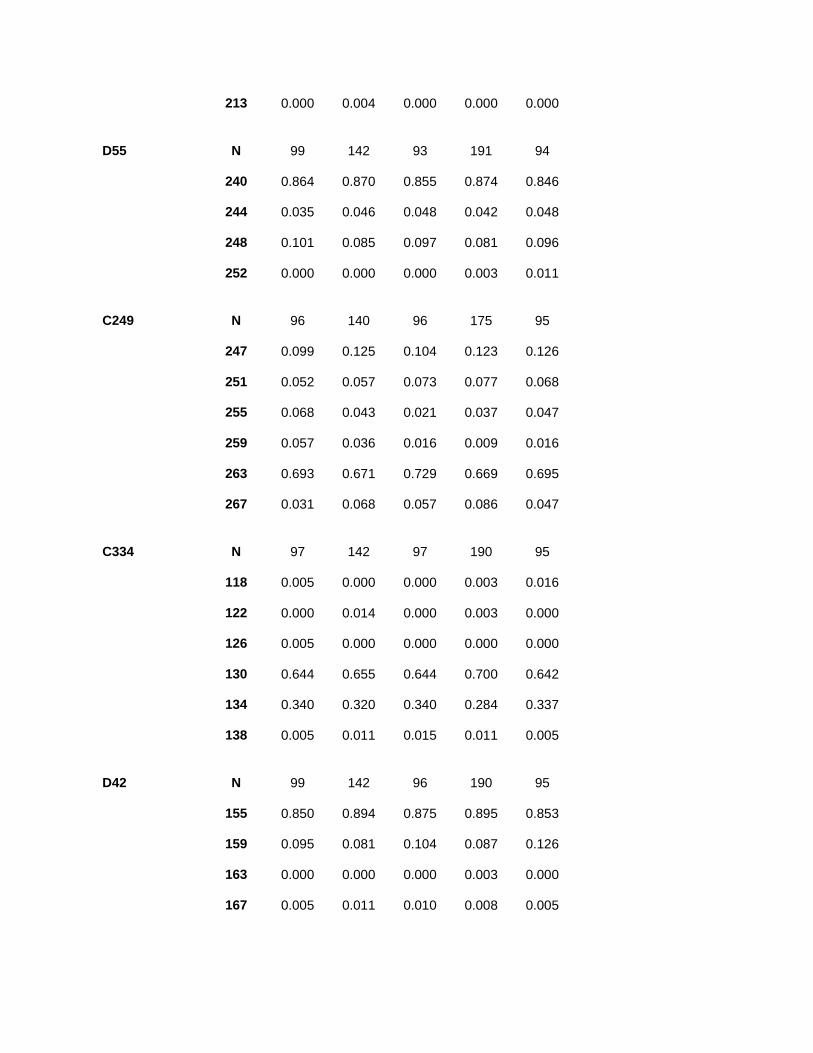
Appendix. Allele frequencies and sample size of Alabama shad microsatellite loci for each sampling year.

Locus Allele/n 2005 2008 2009 2010 2011

D21 N 52 96 97 171 93

275 0.010 0.000 0.010 0.003 0.000

279 0.029 0.005 0.005 0.003 0.005

287 0.865 0.828 0.799 0.816 0.833

291 0.077 0.141 0.139 0.149 0.129

303 0.019 0.026 0.046 0.029 0.032

D30 N 99 142 97 186 93

96 0.000 0.000 0.005 0.000 0.000

100 0.000 0.000 0.015 0.000 0.000

116 0.025 0.074 0.067 0.046 0.070

120 0.005 0.007 0.000 0.000 0.005

124 0.010 0.014 0.021 0.008 0.011

132 0.778 0.782 0.747 0.777 0.763

136 0.035 0.021 0.015 0.030 0.043

140 0.101 0.067 0.082 0.102 0.075

144 0.025 0.025 0.026 0.030 0.027

148 0.000 0.000 0.000 0.003 0.000

152 0.020 0.011 0.021 0.005 0.005

D31 N 99 142 97 184 94

198 0.995 0.993 1.000 0.995 0.995

210 0.005 0.007 0.000 0.005 0.005

D429 N 99 141 96 184 93

126 0.000 0.007 0.010 0.000 0.000

146 0.495 0.652 0.917 0.916 0.935

150 0.030 0.035 0.073 0.084 0.065

154 0.409 0.270 0.000 0.000 0.000

158 0.061 0.035 0.000 0.000 0.000

166 0.005 0.000 0.000 0.000 0.000

B20 N 100 144 94 191 93

110 0.010 0.010 0.021 0.010 0.005

114 0.095 0.080 0.090 0.099 0.097

122 0.895 0.910 0.888 0.890 0.898

D312 N 100 143 94 191 94

142 0.005 0.007 0.005 0.005 0.005

146 0.020 0.004 0.005 0.008 0.011

150 0.010 0.014 0.021 0.016 0.011

154 0.000 0.004 0.005 0.008 0.016

158 0.195 0.178 0.186 0.152 0.138

162 0.280 0.325 0.303 0.348 0.351

166 0.140 0.196 0.160 0.152 0.154

170 0.140 0.077 0.101 0.081 0.106

174 0.085 0.017 0.059 0.050 0.037

178 0.050 0.056 0.032 0.050 0.053

182 0.045 0.052 0.069 0.092 0.064

186 0.000 0.014 0.011 0.005 0.005

190 0.015 0.014 0.021 0.016 0.021

194 0.000 0.010 0.000 0.005 0.011

198 0.000 0.000 0.005 0.003 0.000

202 0.010 0.021 0.016 0.010 0.011

206 0.005 0.004 0.000 0.000 0.005

209 0.000 0.004 0.000 0.000 0.000

213 0.000 0.004 0.000 0.000 0.000

D55 N 99 142 93 191 94

240 0.864 0.870 0.855 0.874 0.846

244 0.035 0.046 0.048 0.042 0.048

248 0.101 0.085 0.097 0.081 0.096

252 0.000 0.000 0.000 0.003 0.011

C249 N 96 140 96 175 95

247 0.099 0.125 0.104 0.123 0.126

251 0.052 0.057 0.073 0.077 0.068

255 0.068 0.043 0.021 0.037 0.047

259 0.057 0.036 0.016 0.009 0.016

263 0.693 0.671 0.729 0.669 0.695

267 0.031 0.068 0.057 0.086 0.047

C334 N 97 142 97 190 95

118 0.005 0.000 0.000 0.003 0.016

122 0.000 0.014 0.000 0.003 0.000

126 0.005 0.000 0.000 0.000 0.000

130 0.644 0.655 0.644 0.700 0.642

134 0.340 0.320 0.340 0.284 0.337

138 0.005 0.011 0.015 0.011 0.005

D42 N 99 142 96 190 95

155 0.850 0.894 0.875 0.895 0.853

159 0.095 0.081 0.104 0.087 0.126

163 0.000 0.000 0.000 0.003 0.000

167 0.005 0.011 0.010 0.008 0.005

179 0.050 0.014 0.010 0.008 0.016

D392 N 100 144 93 182 92

254 0.015 0.003 0.005 0.003 0.011

258 0.300 0.271 0.210 0.266 0.201

274 0.040 0.059 0.070 0.033 0.054

278 0.000 0.007 0.011 0.003 0.000

282 0.575 0.580 0.602 0.585 0.663

286 0.010 0.007 0.000 0.003 0.005

290 0.010 0.021 0.038 0.003 0.005

294 0.005 0.010 0.000 0.027 0.005

298 0.045 0.042 0.065 0.077 0.054