University of Pennsylvania University of Pennsylvania

ScholarlyCommons ScholarlyCommons

Technical Reports (CIS) Department of Computer & Information Science

April 1990

Estimation of General Rigid Body Motion From a Long Sequence Estimation of General Rigid Body Motion From a Long Sequence

of Images of Images

Siu-Leong Iu University of Pennsylvania

Kwangyoen Wohn University of Pennsylvania

Follow this and additional works at: https://repository.upenn.edu/cis_reports

Recommended Citation Recommended Citation Siu-Leong Iu and Kwangyoen Wohn, "Estimation of General Rigid Body Motion From a Long Sequence of Images", . April 1990.

University of Pennsylvania Department of Computer and Information Science Technical Report No. MS-CIS-90-22.

This paper is posted at ScholarlyCommons. https://repository.upenn.edu/cis_reports/524 For more information, please contact repository@pobox.upenn.edu.

Estimation of General Rigid Body Motion From a Long Sequence of Images Estimation of General Rigid Body Motion From a Long Sequence of Images

Abstract Abstract In estimating the 3-D rigid body motion and structure from time-varying images, most of previous approaches which exploit a large number of frames assume that the rotation, and the translation in some case, are constant. For a long sequence of images, this assumption in general is not valid. In this paper, we propose a new state estimation formulation for the general motion in which the 3-D translation and rotation are modeled as the polynomials of arbitrary order. Extended Kalman filter is used to find the estimates recursively from noisy images. A number of simulations including the Monte Carlo analysis are conducted to illustrate the performance of the proposed formulation.

Comments Comments University of Pennsylvania Department of Computer and Information Science Technical Report No. MS-CIS-90-22.

This technical report is available at ScholarlyCommons: https://repository.upenn.edu/cis_reports/524

Estimation Of General Rigid Body Motion From A Long Sequence

Of Images

MS-CIS-90-22 GRASP LAB 204

Siu-Leong Iu Kwangyoen Wohn

Department of Computer and Information Science School of Engineering and Applied Science

University of Pennsylvania Philadelphia, PA 19104-6389

April 1990

ESTIMATION OF GENERAL RIGID BODY MOTION FROM A LONG

SEQUENCE OF IMAGES

Siu-Leong Iu & Kwangyoen Wohn

The Grasp Laboratory School of Engineering and Applied Science

University of Pennsylvania Philadelphia, PA 19 104.

Abstract

In estimating the 3-D rigid body motion and structure from time-varying images, most of previous approaches which exploit a large number of frames assume that the rotation, and the translation in some case, are constant. For a long sequence of images, this assumption in gen- eral is not valid. In this paper, we propose a new state estimation formulation for the general motion in which the 3-D translation and rotation are modeled as the polynomials of arbitrary order. Extended Kalman filter is used to find the estimates recursively from noisy images. A number of simulations including the Monte Carlo analysis are conducted to illustrate the per- formance of the proposed formulation.

Key words: Image motion analysis, structure from motion, extended Kalman filter.

Acknowledgement: This research was supported in part by DARPA grant N00014-88-K- 0632, NSF equipment grant CCR-87 16975 and NSF grant IRI89-06770.

Page 2

1. INTRODUCTION

Token-matching approach and optical flow approach are two kinds of approaches to the recovery of 3-

D motion and structure from images by using, respectively, the measurement of projective position

[Agga81, Lin86, Seth87, Fang84, Rana801 and the measurement of optical flow [Ullrn81, Hom81,

Wohn83, Hild83, Nage83, Schu85, Heeg861. Our work described in this paper belongs to the token-

matching approach. For the token matching approach, point features in the scene have been studied

extensively [Ullrn79, Roac80, Nage81, Long81, Huan81, Tsai84, Faug87, Nage861. Other features like

line segments and conic arc in the scene have also been used [Liu86, Miti86, Faug87, Tsai831. For the

optical flow approach, 3-D motion is determined from the measurement of optical flows, and its tem-

poral and spatial derivatives [Long80, Waxm85, Long84, Subb85, Kana85, Waxm86, Wu861.

Aggarwal and Nandhakumar [Agga88] gave an excellent and up to date review of the whole field of

estimating the 3-D structure and motion from sequences of monocular and stereoscopic images.

Most of existing structure-from-motion algorithms which utilize a small number (two or three) of

frames perform poorly under the presence of noise in the measurement. Recently, a number of

researchers [Weng87, Broi86a,b, Bo1185, Iu89a, Broi89, Kuma891 have proposed to use a large number

of frames in order to improve the estimation performance. The very first step towards the "multi-

frame" analysis is to model the kinematic variables of moving object during an extended period of

time. As far as the translational motion is concerned, the trajectory w.r.t. time describes the motion

completely. Since an object can move almost arbitrarily in front of a camera, we do not know this tra-

jectory explicitly. However, according to Weierstrass approximation theorem, we can approximate any

continuous trajectory over a closed and bounded time interval by using polynomials. In practice, we

can only use low order polynomials because of the numerical stability and the real-time constraints. If

the object moves in the 3-D space smoothly, such low order polynomials may be good enough in

describing its motion locally. Note that the projectile motion of a throwing ball can be represented by

using second order polynomials. In the following we contrast our approach to the two previous work

which is considered as the major contribution to our understanding of motion estimation from a long

sequence of images.

Weng, Huang and Ahuja [Weng87] proposed the locally constant angular momentum model in

estimating 3-D motion from the measurements of projective positions. Their model assumed that angu-

lar momentum was constant over a short time interval, the moving body possessed an axis of syrn-

metry and the motion of the rotation center was approximated as a polynomial. The first two assump-

tions are required in their derivation because they wanted the Euler's equations integrable. In our

Page 3

approach, we do not make these two assumptions because we directly derive the relation between the

unknown motion parameters and the projective positions, rather than solving the equations involving

the external torque and the angular momentum. In finding the 3-D motion, they first estimated the rota-

tion matrices and the translation between the frames by using "two-frame" motion analysis, and then

determined the motion of the rotation center, i.e., their approach considers each frame separately. In

our approach, we utilize all the available information in the temporal and spatial domains to estimate

the translation velocity of the rotation center, the rotation of the rigid body and the relative depth

simultaneously. Furthermore, in their paper, only simulations on binocular image sequences were

reported.

Broida and Chellappa [Broi86a,b] estimated motion parameters sequentially from the projective

position of multiple points in a sequence of noisy images. They used a dynamic model to describe the

temporal behavior of parameters and employed the iterative extended Kalrnan filter to estimate them.

In [Broi86a], they estimated the motion of a two-dimensional object from its one-dimensional projec-

tions. They assumed that the image coordinates of feature points were available, that the motion was

unforced, that the absolute distance to the center of rotation was known and that the noise level in the

Kalrnan filter formulation was known. In [Broi86b], they extended their work to 3-D rigid body

motion. Quaternions were used to describe the rotation. Motion was modeled by a truncated Taylor

series but only the linear term was used in their derivation. Simulations on very special motion only,

such as pure translation or rotation about a fixed and known axis, were reported in their paper. In

[Broi86c], they used batch approach to find the estimate. Their result on uniqueness of rigid body

motion was limited to the pure translational motion [Broi89]. For the non-constant rotation, numerical

integration was proposed [Broi86b,c, Broi891 but neither specific algorithms nor experiments were

given.

Iu and Wohn [Iu89a] argued that the estimation of motion should exploit the temporal informa-

tion from images first rather than seeking for the motion constraint from the spatial domain. They

showed that the 3-D velocity of a single point up to a scalar factor could be recovered from images

and proved the uniqueness of solution for the case that the 3-D velocity is modeled as an arbitrary

order of polynomials. Regression relation between unknown motion parameters and measurements

from noisy images was derived and the batch approach was used to find the optimal estimate under the

criterion of Maximum Likelihood. They also extended their work to 3-D rigid body motion with con-

stant angular velocity. In [Iu89b], extended Kalman filter was used to estimate the motion sequen-

tially.

Page 4

We have observed that most of the previous approaches modeled the rotation, and the translation

for some cases, as a constant. One may attempt to extend the analysis for the constant motion to the

one for the general motion by expanding the translational and the rotational parameters in polynomials

and plugging them into the original formulation of the constant motion. However, for the rotational

motion, although we can still use a higher order polynomials to describe the rotation, the state equation

relating the rotation and the 3-D trajectory of the feature points respect to the rotational center is time

varying. Since there is no explicit closed form solution for this equation, the previous approaches were

not able to handle the non-constant rotational motion effectively. In this paper, we propose a new state

estimation formulation in which the explicit solution of the above state equation is not required. Conse-

quently, the analysis can include the object motion with arbitrary orders of translation and rotation.

The rest of the paper is organized as follows. Section 2 describes the model of general rigid body

motion. Section 3 gives the state estimation formulation. The motion with constant acceleration is dis-

cussed first. Section 4 gives the result of simulations. Some concern on generating the test data is also

pointed out. Section 5 is the conclusion of this paper with discussion.

Page 5

2. MODEL OF RIGID BODY MOTION

Suppose that there are n, feature points on the visible surface of the rigid object and that we have

measured the projected position of these points as the object moves in front of a camera. It is well

known that any rigid body motion can be represented by the translation of the rotational center and the

rotation of the entire object with respect to this rotational center. We also know that we can only

recover the translation up to a scale factor because of the perspective projection. Thus, our objective is

to find this translation of the rotational center up to the scalar factor and the rotation from the observed

projected positions.

Let $(t) = [Xi(t) Yi(t) zi(t)lT, ~ ( t ) = [xi(t) yi(t)lT and x( t ) = [Vxi(t) VYi(t) vZi(t)lT be the 3-D position,

the projected position and the instantaneous velocity of i-th feature point at time t, respectively. The

symbol 'T' denotes the transpose of a vector. Then we have

Note that we have used the pin-hole camera model and have scaled the Z-axis such that the focal

length is normalized to one [Long80]. Let ;Z(t) = [Q,(t) QY(t) QZ(t)lT be the angular velocity of the

object respect to the rotational center Po(t). - From the assumption of rigidity, we have

where the symbol 'x' denotes the cross product of vectors. We can express (2.3) alternatively in the

following form:

If the object moves smoothly in the 3-D space, we may model the translation and the rotation as the

following polynomials with orders d, and d, respectively.

Page 6

where @'](to) = [ xrnl(to> Y["I(~) Z["I(~) lT and @"](to) = [ i2g1(to) !2F1(t,,) i2P1(to) lT are the n-th deriva-

tives of Eo(t) and g(t) evaluated at time t = to. Note that gho1(k) = co(to) and @[O1(t,,) = Q(t,,). The physi-

cal interpretation of Ehll(b) and gh21(b) are the velocity and acceleration of translation at time to, respec-

tively. The g[O1(to) and at1](b) - are the angular velocity and acceleration of rotation at time t,,, respec-

tively. Then our goal is to estimate the translational coefficients PR](~~J, - n = 0, 1, . - , d, in (2.6) scaled

by the factor representing the absolute depth and rotational coefficients @"](to), n = 0, 1, - . , d, in

(2.7), from the measurement of ~ ( t ~ ) , i = 0, - - . , n, - 1, j = 0, 1, . . - . If the rotation is constant, i.e., - Q(t) = Q(t,-,), - then A(t) is a constant matrix and the state equation

(2.4) has the close-form solution

where e A [ t - b l is the state transition matrix and eAt is equal to the inverse Laplace transform of

(sI - A)-'. Then the rigid body motion can be determined by solving the regression problem [Iu89a] or

the state estimation problem [Broi86b]. Unfortunately, if the rotation is time varying, there is in general

no closed-form expression for [ E(t) - Po(t) - ] in terms of - Q(t) and [ E(t,,) - gflt,,) ] because of the time-

varying nature of A(t) [Iu89aj. This is why one can not extend the derivation of the previous

approaches [Iu89a, Broi86bl to the general motion in a straightforward manner. In this paper, we

develop a state estimation formulation in which the explicit solution of (2.4) is not required, given an

arbitrary order of rigid body motion.

3. STATE ESTIMATION FORMULATION AND RECURSIVE SOLUTION

The problem of recovering general rigid body motion will be formulated as the state estimation prob-

lem. Let ~ ( t ) be the state vector which is composed of the unknown motion parameters. Let - m(tj) be the

measurement vector which is formed by the available measurements from the image at time tj;

where - n(tj) is a discrete-time random process describing the noise in the measurements. The com-

ponents of ~( t . ) are assumed to be independent and ( - n(tj), j = 0, 1, . e . ) are assumed to be white zero

mean Gaussian random vectors with common variance matrix. If we can derive the state evolution and

the relation between the measurement and state vectors in the following plant equation and measure-

ment equation,

Page 7

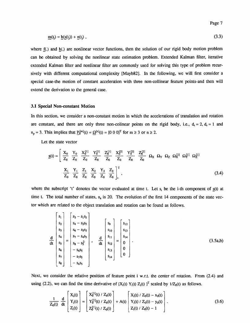
where - f(.) and - h(.) are nonlinear vector functions, then the solution of our rigid body motion problem

can be obtained by solving the nonlinear state estimation problem. Extended Kalman filter, iterative

extended Kalman filter and nonlinear filter are commonly used for solving this type of problem recur-

sively with different computational complexity [Mayb82]. In the following, we will first consider a

special case-the motion of constant acceleration with three non-collinear feature points-and then will

extend the derivation to the general case.

3.1 Special Non-constant Motion

In this section, we consider a non-constant motion in which the accelerations of translation and rotation

are constant, and there are only three non-colinear points on the rigid body, i.e., d, = 2 , 4 = 1 and

n, = 3. This implies that ~I"l(t) - = - i2rnl(t) = [O 0 OIT for m 2 3 or n 2 2.

Let the state vector

where the subscript 't' denotes the vector evaluated at time t. Let q be the i-th component of ~ ( t ) at

time t. The total number of states, n, is 20. The evolution of the first 14 components of the state vec-

tor which are related to the object translation and rotation can be found as follows.

Next, we consider the relative position of feature point i w.r.t. the center of rotation. From (2.4) and

using (2.2), we can find the time derivative of [Xi@) Yi(t) &(t) lT scaled by l/Zo(t) as follows.

Page 8

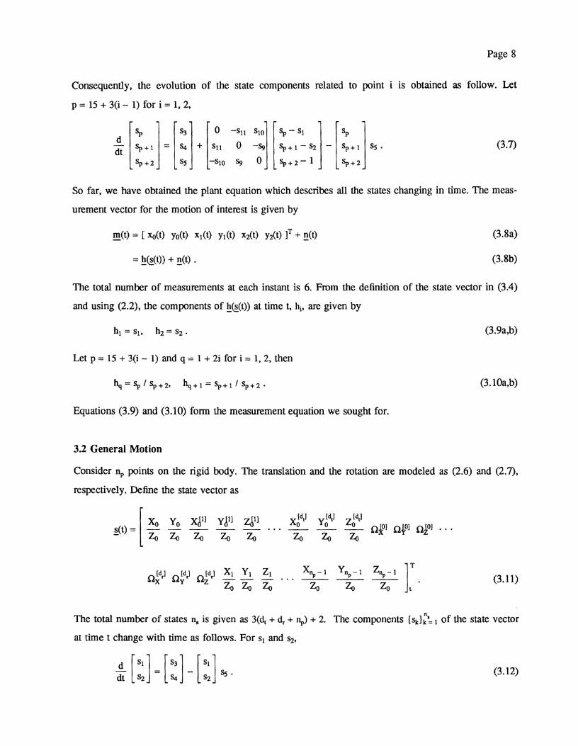
Consequently, the evolution of the state components related to point i is obtained as follow. Let

p = 15 + 3(i - 1) for i = 1, 2,

So far, we have obtained the plant equation which describes all the states changing in time. The meas-

urement vector for the motion of interest is given by

The total number of measurements at each instant is 6. From the definition of the state vector in (3.4)

and using (2.2), the components of ljs(t)) at time t, hi, are given by

Let p = 15 + 3(i - 1) and q = 1 + 2i for i = 1,2, then

Equations (3.9) and (3.10) form the measurement equation we sought for.

3.2 General Motion

Consider n, points on the rigid body. The translation and the rotation are modeled as (2.6) and (2.7),

respectively. Define the state vector as

The total number of states n, is given as 3(4 + 4 + %) + 2. The components ( s k ] 2 of the state vector

at time t change with time as follows. For sl and s2,

Page 9

For the states which represent the translational motion, let p = 3 + 3(i - 1) for i = 1, . . . , dt - 1,

For the states which represent the rotational motion, let p = (34 + 3) + 3i for i = 0, . . - , 4 - 1,

For the states which represent the location of feature points, let p = (34 + 3 4 + 6) + 3(i - 1) for

i = l , - . . , n , - 1,

I;.] = [a::]. t dt + 2 + 5

Using the definitions of state vector and measurement vector in (3.11) and (3.1), we can obtain the

measurement equation in the form of (3.3) with the following components of &&(t,)), (h,~:: ,, where n,

is the total number of measurements at each time and equals to 2n,.

Let p = (34+ 3 4 + 6) + 3(i - 1) and q = 1 + 2i for i = 1, - - 0 , n,- 1,

hq=Sp/Sp+2> h q + 1 = s p + 1 / s p + 2 -

- S34+3d1+3

s34+.+4

s34+3dr+5 L

In summary, we obtain the state equation which is formed by (3.12)-(3.15) and the measurement equa-

tion which is given by (3.16)-(3.17) for the general rigid body motion. Thus, the estimation of the gen-

eral motion for a rigid body can be obtained by solving the nonlinear state estimation problem as we

claimed earlier.

= [n]

4. SIMULATION RESULTS

In order to illustrate the performance of the proposed approach to the motion estimation of the general

rigid body motion, a number of experiments on simulated data are conducted. In the simulation, only

three feature points are used. The focal length of the camera is set to one unit. The visible portion of

Page 10

the image plane is (-0.36, 0.36) x (-0.36, 0.36) units. This portion corresponds to the viewing angle of

k 20 degrees. The observed image is considered as 256 x 256 pixels. We consider the motion of con-

stant acceleration (4 = 2 and d, = 1). The time interval between frames is 0.04 second. To solve the

nonlinear state estimation problem in (3.2) and (3.3) recursively, extended Kalrnan filter is used. The

initial estimates of the translation and rotation are set to zero. The initial estimates of the related depth

of the feature points are set to one.

On generating test data

The noisy measurements of the projected position ~ ( t ) , i = 0, - , npl at different sampling time tj,

j=O, 1, . . . , are generated by adding white zero mean Gaussian noise to the exact values of ~ ( t ) . In

the following, we explain and discuss the procedure of obtaining these exact projected positions from

the given motion parameters: the 3-D position of feature points at time zero, the translational

coefficients pP1(0), - n = 1, . . , d, and rotational coefficients - nl"](0), n = 1, - . . , 4.

At a first glance, one may be tempted to use (3.12)-(3.15) to get the time evolution of state vector

and then use (3.16) and (3.17) to obtain ~ ( t ) at different sampling times. However, since the time evo-

lution of the states in (3.12)-(3.15) is nonlinear and coupled, a system of nonlinear differential vector

equations with a large number of unknowns is required to solve. Although numerical techniques such

as Runge Kutta method can be used to find this solution, the accumulated error may result the large

error in the generated data. This is especially true when a large number of frames, say 100 frames, are

involved. In order to overcome this problem, we use another approach. We first obtain the 3-D trajec-

tory of rotational center &(t) at different sampling times by using (2.6) with known P~](O), - n = 1, - . . , d,. The 3-D trajectory of individual feature point, s(t), is determined by solving the state

equation (2.4) and adding the result to - Po(t). Note that A(t) in (2.4) at any time can be found by using

(2.7) with known - Q["](o), n = 1, - . - ,4. The state equation (2.4) is time-varying but it is not nonlinear.

Also, there are only three unknowns in the equation. Runge Kutta method is used to solve the equa-

tion. Then the exact projected positions are obtained by using the perspective relation in (2.2).

Experiment 1: Various noisy levels

In this experiment, we compare the estimates at different noisy levels. The standard deviations of the

noise are set to 0.5, 2.5 and 5 pixels. The 3-D translation gJ1](t) is [ -1 5 10 lT + [ -0.05 -2.5 -5 lT t

unitslsecond. The 3-D angular velocity - Q(t) is [ -0.4 0.5 3 lT + [ 0.1 -0.3 -1.7 lT t radianslsecond. The

3-D positions of the three feature points at time zero are (4, -2, 20), (5, -5, 19.5) and (3, -5, 20.5)

Page 11

units. Figure l a shows the images of the simulated motion at every five frames. Figure l b shows the

exact and noisy trajectories of the first three feature points on the image plane (Only the trajectory with

2.5 pixel error is shown). Figures l c and Id are the x and y components of the trajectory, respec-

tively. Figures le-11 are the exact and estimated x,J11(t)/zo(t), ~,J'l(t)/z~(t), all(t)iZo(t), Qx(t), a&), Qz(t),

Zl(t)/Zo(t) and Z2(t)/Zo(t), respectively. From these results, we observed that the estimated errors

decrease as the noise in the measurements decrease. The estimate errors for xi1] / Zo(t) and YJ'] / Z,-,(t)

are smaller than that for z,J11 / zo(t). The estimate of rotations in X and Y direction are worst than that

in Z direction. The estimate of relative depths can follow the change of the movement. As we use

more frames, the estimate error decreases. For the case of 2.5 pixel error in the measurements, it takes

about 60 frames to converge. This observation period is less than 2.5 seconds. Note that the estimate

error is very large if we only use a smaller number of frames. This justifies that motion analysis using

a small number of frames performs badly if there is noise in the measurements. We have similar

observations discussed above for the following Monte Carlo analysis.

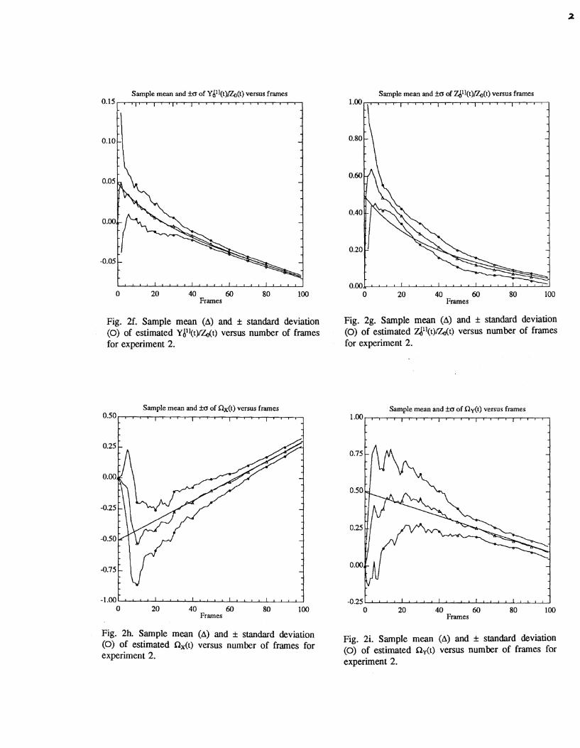
Experiment 2: Monte Carlo analysis

In this experiment, we run the simulation for fifty different sets of noise and compute the sample mean

and standard deviation of the estimates . The standard deviation of the noise is 2.5 pixels. The 3-D

translation zJ1](t) is [ -3 1 10 lT + [ 1 -1 -2 lT t unitslsecond. The 3-D angular velocity @(t) is

[ -0.5 0.5 2 lT + [ 0.2 -0.1 -1.4 lT t radianslsecond. The 3-D positions of the particles at time zero are

(0, 0, 20), (4, -4, 19.5) and (-2, -4, 20.5) units. Figure 2a shows the images of the simulated motion at

every five frames. Figures 2b, 2c and 2d show the exact and a typical noisy trajectories, and their x

and y components. Figures 2e-21 show the sample mean and the rt 1 standard deviation of the

estimated x6l1(t)tZ0(t), ~6l](t)/Z~(t), Z6l1(t)/z0(t), Qx(t), Qy(t), aZ(t), Zl(t)iZo(t) and &(t)/Zo(t) versus

number of frames used in the estimation, respectively. It is observed that the sample mean converges

to the true values and the sample standard deviations decrease as we use more frames.

5. CONCLUSION

We have proposed a new state formulation to analyze the object motion with arbitrary orders of trans-

lation and rotation from a sequence of video images. Extended Kalrnan filter was used to find the esti-

mate recursively. The simulations showed that the proposed formulation was quite effective for

estimating the non-constant rigid body motion, even the measurements had 5 pixels error. This formu-

lation may be adopted with minor modification to the motion analysis for other measurements, such as

the sequences of stereo images, spatially distributed infrared image, and radar observations of range

Page 12

and bearings [Mayb82].

We may follow the derivations in this paper with modification to formulate the general rigid body

motion in terms of quaternions [Broi86b]. However, we need to solve an additional time-varying 4x1

vector differential equation in order to obtain the quaternions at different instant from the non-constant

angular velocity. Also, a non-linear algebra transformation is required to relate the estimated states to

the measurements. These will increase the computational complexity and the additional error in the

numerical integration.

For the model of rigid body motion we used, we assumed that the projective position of rota-

tional center is visible, that the motion is smooth, and that the orders of the translation and rotation are

known. Note that these assumptions are also used in [Weng87] and [Broi89]. For the first assurnp-

tion, if the rotational center belongs to one of the feature points but we do not know which point is,

one may regard each point as the rotational center, and apply the estimation procedure to each case.

This approach is not unrealistic since the number of feature points we observed is commonly small and

all the procedures can be processed simultaneously. Another approach is to detect the rotational center

from the observed points and then estimate the motion. On the other hand, if the feature points do not

contain the rotational center, then the method is not applicable directly.

In regard to the other two assumptions, since the object can move almost arbitrarily in front of a

camera, the order of polynomials in describing the true motion may not match to the model exactly.

Also, the object may change its motion abruptly. One such example is a ball bouncing off the ground.

This situation leads us to consider three classes of model mismatch: undermodeling, overmodeling and

parameter jumping. We have analyzed the performance degradation due to these model mismatches and

proposed the Finite Lifetime Alternately Triggered Multiple Model Filter @TAT MMF), as a new solu-

tion. This issue is dealt in [Iu89b, Iu90aI.

Page 13

Reference

[Agga8 11 J.K. Aggarwal, L.S. Davis and W.N. Martin, "Correspondence process in dynamic scene analysis", Proc. of IEEE, 1981, pp. 562-572.

lAgga881 J.K. Aggarwal and N. Nandhakumar, "On the computation of motion from sequence of image- a review", Proc. of IEEE, August 1988, pp. 917-935.

[Boll851 R.C. Bolles and H.H. Bakers, "Epipolar-plane image analysis: a technique for analyzing motion sequences", in Workshop on computer vision: representation and control, Oct. 1985.

[Broi86a] TJ. Broida and R.Chellappa, "Estimation of object motion parameters from noisy images", IEEE PAMI, January 1986 , pp. 90-99.

[Broi86b] TJ. Broida and R. Chellappa, "Kinematics and structure of a rigid object from a sequence of noisy images", IEEE Workshop on visual motion 1986, pp. 95-100.

[Broi86cl T.J. Broida and R. Chellappa, "Kinematics and structure of a rigid object from a sequence of noisy images: A batch approach", Proc. IEEE Conf. Computer Vision and Pattern Recognition, Miami Beach, FL, June 1986, pp. 176-182.

[Broi89] TJ. Broida and R. Chellappa, "Experiments and uniqueness results on object structure and kinematics from a sequence of monocular images", IEEE Workshop on visual motion, March 1989, pp. 21-30.

Fang841 J.Q. Fang and T.S. Huang, "Solving three- dimensional small-rotation motion equations : uniqueness, algorithms and numerical results", CVGIP 26, 1984, pp. 183-206.

Faug871 O.D. Faugeras, F. Lustman and G. Toscani, "Motion and structure from motion from point and line matches", To be published, 1987.

[Hild83] E.C. Hildreth, The measurement of visual motion, MIT press, Cambridge, 1983.

EHeeg861 DJ. Heeger, "Depth and flow from motion energy", Science 86, pp. 657-663.

[Horn811 B.K.P. Horn and B.G. Schunck, "Determining optical flow", Artificial Intelligence 17, 1981, pp. 185-204.

[Hum8 11 T.S. Huang and R.Y. Tsai, "Image sequence analysis: Motion estimation", in Image Sequence Processing and Dynamic Scene Analysis, T.S. Huang, Ed. NY: Springer-verlag, 1981.

[Iu89a] S.-L. Iu and K. Wohn, "Estimation of 3-D motion and structure based on a temporally- oriented approach with the method of regres- sion", IEEE Workshop on visual motion, March 1989, pp. 273-281.

[Iu89b] S.-L. Iu and K. Wohn, "Recovery of 3-D motion of a single particle", SPIE Proceedings, Intelli- gent Robots and Computer Vision VIII, Philadel- phia, Nov. 1989, pp. 746-757.

[Iu90a] S.-L. Iu, "Analysis of the effects of model mismatch and FLAT MMF for estimating parti- cle motion", Tech. Report MS-CIS-90-10, GRASP Lab., Univ. of Pennsylvania, Feb. 1990.

[Kuma89] R.V.R. Kumar, A. Tirumalai and R. C. Jain, "A non-linear optimization algorithm for the estima- tion of structure and motion parameters", IEEE Workshop on visual motion, March 1989, pp. 136-143.

[Kana851 K. Kanatani, "Structure from motion without correspondence : general principle", 9th UCAI, pp. 886-888.

Liu861 Y. Liu and T.S. Huang, "Estimation of rigid body motion using straight line correspondences: further results", IEEE ICPR 1986, pp. 306-309.

Lin861 Z.C. Lin, H. Lee and T.S. Huang, "Finding 3-D point correspondences in motion estimation", IEEE ICPR 1986, pp. 303-305.

Long801 H.C. Longuet-Higgins and K. Prazdny, "The interpretation of a moving retinal image", Roc. of Royal Society of London, B208, pp. 385-397.

Long8 1 I H.C. Longuet-Higgins, "A computer algorithm for reconstructing a scene from two projections", Nature 293, pp. 133-135, 1981.

Page 14

[ILong841 H.C. Longuet-Higgins, "The visual ambiguity of a moving plane ", Roc. of Royal Society of London, B223, pp. 165-175.

[Mayb82] P. S. Maybeck, Stochastic models, estimation and control, vol. 1-2, Academic Press, 1982.

[Miti863 A. Mitiche, S. Seida and J.K. Aggarwal, "Line- based computation of structure and motion using angular invariance", Proc. of IEEE Workshop on visual motion : representation and analysis, 1986, pp. 175-180.

W ~ e 8 1 I H.-H. Nagel, " Representation of moving rigid objects based on visual observations", Computer, A u ~ . 1981, pp. 29-39.

mage831 H.-H. Nagel, "Displacement vectors derived £rom second-order intensity variations in image sequences", CVGIP, 1983, pp.85-117.

INage861 H.-H. Nagel, "Image sequences-Ten (octal) years- From phenomenology towards a theoreti- cal foundation", in Proc. Int. Conf. on Pattern Recognition, Oct. 1986, pp. 1174-1185.

IRana801 S. Ranade and A. Rosenfeld, "Point pattern matching by relaxation", Pattern Recognition, V O ~ . 12, 1980, pp. 269-275.

rRoac801 J.W. Roach and J.K. Aggarwal, "Determining the movement of object from a sequence of images", IEEE PAMI, Nov 1980, pp.554-562.

[Schu85] B.G. Schunck, "Image flow: Fundamentals and future research", in Proc. of IEEE Conf. on Pat- tern recognition and Image Processing, 1985, pp. 560-57 1.

[Se ti1871 S.K. Sethi and R. Jain, "Finding trajectories of feature points in a monocular image sequence", IEEE PAMI, Jan. 1987, pp. 56-73.

[Subb85] M. Subbarao and A. M. Waxman, "On the uniqueness of image flow solutions for planar surfaces in motion", IEEE Workshop on com- puter vision: representation and control, Oct 1985, pp. 129-140.

CTsai831 R. Y. Tsai, "3-D inference from the motion

parallax of a conic arc and a point in two per- spective view", IEEE UCA183, pp. 1038-1042.

[Tsai84] R.Y. Tsai and T.S. Huang, "Uniqueness and esti- mation of three-dimensional motion parameters of rigid objects with curved surfaces", IEEE PAMI, Jan 1984, pp. 13-26.

CUllm791 S. Ullrnan, The interpretation of visual motion, Cambridge MIT Press.

Wllrn8 11 S. Ullman, "Analysis of visual motion by biolog- ical and computer systems", IEEE Computer, Aug 1981, pp. 57-69.

[Warn851 A. M. Waxman and S. Ullman, "Surface struc- ture and 3-D motion from image flow : a kinematic analysis", Intl. Journal of Robotics Research 4, 1985, pp. 72-94.

[Warn861 A.M. Waxman, B.Kamgar-Parsi and M. Sub- barao, "Closed-form solutions to image flow equations for 3-D structure and motion", CAR- TR-190, Univ. of Maryland, Feb 1986.

[Weng87] J. Weng, T.S. Huang and N. Ahuja, "3-D motion estimation, understanding and prediction from noisy image sequences", IEEE PAMI, May 1987, pp. 370-389.

[Wohn831 K. Wohn, L.S. Davis and P. Thrift, "Motion esti- mation based on multiple local constraints and nonlinear smoothing", Pattern Recognition 16, 1983, pp. 563-570.

mu861 J. Wu and K. Wohn, "Recovering 3-D motion and structure from 1st-order image deformation", SPIE symposium on intelligent robots, Oct 1986.

Fig. la. Images of simulated motion at every five frames for experiment 1. Last plot includes the trajec- tories on image plane.

Exact and noisy trajectories (2.5 pixels error)

0.24 6

Fig. lb. Exact and noisy trajectories for experiment 1. Standard deviation of the noise is 2.5 pixels.

Exact and noisy measurements of y-component versus frames

0.24

0 20 40 60 80 Frames

100

Fig. Id. Noisy measurements of y-component of the trajectories versus number of frames for experiment 1. Standard deviation of the noise is 2.5 pixels.

Exact and noisy measurements of x-component versus frames , , , , 1 , ' , , , " , ' 1 , , " 1 , , "

-0.244 -0.36 0 20 40 Frames 60 80 100

Fig. lc. Noisy measurements of x-component of the trajectories versus number of frames for experiment 1. Standard deviation of the noise is 2.5 pixels.

Exact and estimated X#l(t)&(t) versus frames

0.20 0

-0.30 0 20 40 60 80 100

Frames

Fig. le. Exact and estimated x6l1(t)/Z0(t) versus number of frames for experiment 1. Standard devia- tions of the noise are 0.5 (O), 2.5 (A) and 5.0 (0) pixels.

Exact and estimated Y~'I(t)lZo(t) versus frames

0

0 20 40 60 80 Frames

100

Exact and estimated Z#](t)&(t) versus frames

-1.00 o o 20 40 Frames 60 80 loo

Fig. If. Exact and estimated YJ1l(t)/&(t) versus Fig. lg. Exact and estimated zdl1(t)/zo(t) versus number of frames for experiment 1. Standard devia- number of frames for experiment 1. Standard devia- tions of the noise are 0.5 (01, 2.5 (A) and 5.0 (0) tions of the noise are 0.5 (a), 2.5 (A) and 5.0 (0) pixels. pixels.

Exact and estimated &(t) versus frames

2.00m

-2.00 I$ 0 20 40 60 80

Frames 1 DO

Fig. lh. Exact and estimated Rx(t) versus number of frames for experiment 1. Standard deviations of the noise are 0.5 (D), 2.5 (A) and 5.0 (0) pixels.

Exact and estimated Ry(t) versus frames

- 2 l l , , , I

0 20 40 60 80 100 Frames

Fig. li. Exact and estimated RY(t) versus number of frames for experiment 1. Standard deviations of the noise are 0.5 (O), 2.5 (A) and 5.0 (0) pixels.

Exact and estimated Qz(t) versus frames " " 1 " " 1 " " 1 " " 1 " "

0 20 40 60 80 100 Frames

Exact and estimated &(t)/&(t) versus frames " ' , 1 ' , ' , 1 , ' , , 1 , , " 1 " "

0.85 0 20 40 60 80 100

Frames

Fig. lj. Exact and estimated Llz(t) versus number of Fig. lk. Exact and estimated Zl(t)/zo(t) versus number frames for experiment 1. Standard deviations of the of frames for experiment 1. Standard deviations of noise are 0.5 (a), 2.5 (A) and 5.0 (0) pixels. , the noise are 0.5 (O), 2.5 (A) and 5.0 (0) pixels.

Exact and estimated Z2(t)&(t) versus frames , , , , 1 , , , , 1 , , , , 1 , , , ,

0 20 40 60 80 100 Frames

Fig. 11. Exact and estimated Z z ( t ) / ~ t ) versus number of frames for experiment 1. Standard deviations of the noise are 0.5 (O), 2.5 (A) and 5.0 (0) pixels.

Fig. 2a. Images of simulated motion at every five frames for experiment 2. Last plot includes the tra- jectories on image plane.

Exact and noisy trajectories

0.366

Fig. 2b. Exact and noisy trajectories for experiment 2. Standard deviation of the noise is 2.5 pixels.

Exact and noisy measurements of y-component versus frames ::;I

-0.24

-0.36 0 20 40 60 80 100

Frames

b a a and noisy measurements of x-component versus frames

0.24 6

Fig. 2d. Noisy measurements of y-component of the trajectories versus number of frames for experiment 2. Standard deviation of the noise is 2.5 pixels.

0 20 40 60 80 100 Frames

Fig. 2c. Noisy measurements of x-component of the trajectories versus number of frames for experiment 2. Standard deviation of the noise is 2.5 pixels.

Sample mean and Am of Xdll(t)&(t) versus frames

0.05 5

- 0 . 2 0 ~ ~ t 1 ~ ~ s ~ ~ 0 ' ~ 9 ~ ~ ~ ~ ~ ~ ~ ~ ~ ~ ~ 1 J 0 20 40 60 80 100

Frames

Fig. 2e. Sample mean (A) and +- standard deviation (0) of estimated x6l1(t)/Zo(t) versus number of frames for experiment 2.

Sample mean and ko of Ydl](t)&,(t) versus frames 0.15, , , , , , , , , , , , , , , , , , , ,

0 20 40 60 80 100 Frames

Fig. 2f. Sample mean (A) and f standard deviation (0) of estimated YJ11(t)/Zo(t) versus number of frames for experiment 2.

Sample mean and of Qx(t) versus frames 0.50

0.25

0.00

-0.25

-0.50

4.75

- 1 . m . ~ ~ ~ ~ ~ ~ l . ~ ' ~ ~ ~ . 1 1 1 1 1 1 1 , , 1

0 20 40 60 80 100 Frames

Fig. 2h. Sample mean (A) and * standard deviation (0) of estimated &(t) versus number of frames for experiment 2.

Sample mean and fo of Z#](t)/&(t) versus frames

l ' " ~ l l " " ' " " l r r l ' ~ ~ ' ~ " " ' I

0 20 40 60 80 100 Frames

Fig. 2g. Sample mean (A) and k standard deviation (0) of estimated Z#'(t)/Zo(t) versus number of frames for experiment 2.

Sample mean and L-a of Qy(t) versus frames

l.ww

0 20 40 60 80 100 Frames

Fig. 2i. Sample mean (A) and * standard deviation (0) of estimated Ry(t) versus number of frames for experiment 2.

Sample mean and of RZ(t) versus frames

0 20 40 60 80 100 Frames

Sample mean and +a of Zl(t)/Zo(t) versus frames 1.05

1.00

0.95

0.90

0.85 0 20 40 60 80 100

Frames

Fig. 2j. Sample mean (A) and * standard deviation Fig. 2k. Sample mean (A) and * standard deviation (0) of estimated Rz(t) versus number of frames for (0) of estimated Zl(t)lZo(t) versus number of frames experiment 2. for experiment 2.

Sample mean and h~ of Zz(t)&,(t) versus frames 1.10 , , , , , , , , , , , , , , , , , , ,

0.95 0 20 40 60 80 100

Frames

Fig. 21. Sample mean (A) and k standard deviation (0) of estimated Zz(t)/Zo(t) versus number of frames for experiment 2.