Estimation of Dynamic Term Structure Models

Gregory R. Duffee and Richard H. Stanton∗

June 8, 2012

ABSTRACTWe study the finite-sample properties of some of the standard techniques used to estimate

modern term structure models. For sample sizes and models similar to those used in mostempirical work, we reach three surprising conclusions. First, while maximum likelihood workswell for simple models, it produces strongly biased parameter estimates when the modelincludes a flexible specification of the dynamics of interest rate risk. Second, despite havingthe same asymptotic efficiency as maximum likelihood, the small-sample performance ofEfficient Method of Moments (a commonly used method for estimating complicated models)is unacceptable even in the simplest term structure settings. Third, the linearized Kalmanfilter is a tractable and reasonably accurate estimation technique, which we recommend insettings where maximum likelihood is impractical.

JEL classification: C14, C52, G12, G13.

∗Duffee is with the Department of Economics, Johns Hopkins University. Stanton is with the Haas Schoolof Business, U.C. Berkeley. We gratefully acknowledge helpful comments and suggestions from Darrell Duffie,Ron Gallant, Bin Gao, Eric Renault, George Tauchen, and seminar participants at Carnegie Mellon, Cornell,Stanford, Stockholm School of Economics, U.C. Berkeley, University of Southern California, Wharton, Yale,the Federal Reserve Bank of San Francisco, Moody’s KMV, and the 2000 Duke Conference on Risk Neutraland Objective Probability Distributions. We are also grateful for financial support from the Fisher Centerfor Real Estate and Urban Economics.

1 Introduction

Starting with Vasicek (1977) and Cox, Ingersoll, and Ross (1985), an enormous literature

has focused on building and estimating dynamic models of the term structure. By specifying

particular functional forms for both the risk-neutral dynamics of short-term interest rates

and the compensation investors require to bear interest rate risk, these models describe

the evolution of yields at all maturities. Much of the literature focuses on the affine class

characterized by Duffie and Kan (1996). This class allows multiple state variables to drive

interest rates and has the computationally convenient feature that bond yields are linear

functions of these variables. The first generation of affine models, including multivariate

generalizations of Vasicek and Cox et al., imposed two specializing assumptions: the state

variables are independent and the price of risk is a multiple of interest rate volatility. Given

these restrictions, estimation of the models’ parameters is reasonably simple.

The estimation results revealed limitations in the models. For example, Dai and Singleton

(2000) find strong evidence of nonzero correlations among the state variables. Duffee (2002)

finds that the restriction on the price of risk implies unrealistic behavior for bonds’ excess

returns. Moreover, there is evidence of nonlinearity in expected interest rate movements

that is inconsistent with these models.1 In response to these limitations, researchers have

introduced more flexible, “second generation” models. For example, Dai and Singleton

(2000) estimate affine models in which the state variables are allowed to be correlated, while

retaining the assumption that the price of risk is proportional to volatility. Duffee (2002)

constructs a multifactor affine model with a more general specification for the dynamics of

the price of risk than in Dai and Singleton (2000). Duarte (2004), Ahn, Dittmar, and Gallant

(2002), and Leippold and Wu (2002) construct models with fairly general specifications of

the price of risk that produce nonlinear dynamics.2

Although these new models are a significant improvement over earlier models, their ability

to capture the observed dynamics of bond yields is not yet clear because the corresponding

empirical literature is relatively immature. This is due to both the quick pace of the model-

ing advances and the difficulty of estimating some of these more complex models. Maximum

likelihood is asymptotically efficient, but its finite-sample properties in the context of these

models are not clear. Moreover, for many of these models the probability distribution of

discretely sampled bond yields is unknown or intractable. Alternative techniques include

1Nonlinearities are documented in Pfann, Schotman, and Tschernig (1996), Aıt-Sahalia (1996), Conley,Hansen, Luttmer, and Scheinkman (1997), and Stanton (1997).

2Other nonlinear models include Longstaff (1989), Beaglehole and Tenney (1992), Constantinides (1992),and Ahn and Gao (1999). The latter two have prices of risk that are more flexible than those in Dai andSingleton (2000). Stanton (1997) and Boudoukh, Downing, Richardson, Stanton, and Whitelaw (2010) arenonparametric (and therefore nonlinear) models of both physical drifts and prices of risk.

1

moment-based methods and simulation methods. The optimal technique is difficult to de-

termine due to our limited understanding of the properties of these techniques when applied

to sophisticated term structure models.

In this paper we study the finite-sample properties of three prominent techniques used

to estimate second-generation term structure models, in settings close to those facing re-

searchers estimating these models. The first technique we study is maximum likelihood (the

method of choice when the state variables can be precisely inferred by the econometrician),

used, for example, by Pearson and Sun (1994), Chen and Scott (1993), Aıt-Sahalia and

Kimmel (2010), and Brandt and He (2002). We employ exact maximum likelihood when

the likelihood function is known, and simulated maximum likelihood when it is not, using

the method of Pedersen (1995) and Santa-Clara (1995). The second technique we study

is the Efficient Method of Moments of Gallant and Tauchen (1996) (used, for example, by

Dai and Singleton, 2000; Ahn et al., 2002; Andersen and Lund, 1997; Gallant and Tauchen,

1997). It is the most widely used alternative when maximum likelihood is infeasible, be-

cause it is tractable and can attain the same asymptotic efficiency as maximum likelihood.

This technique uses an auxiliary model. We follow common practice by choosing a semi-

nonparametric model; thus we refer to this technique as EMM/SNP. The final method is a

variant of the Kalman filter. This may or may not be maximum likelihood, depending on

the setting. For each technique, we use Monte Carlo simulations to determine the behavior

of the estimators for sample sizes and models similar to those used in most empirical work.

To keep the size of the paper manageable, we restrict our attention to models in the affine

class with independent factors. We examine models in both the “essentially affine” class of

Duffee (2002) and the “semi-affine” class of Duarte (2004).

Though we consider only a few of the infinite number of possible models, our results

allow us to draw three main conclusions that apply much more generally. Each stands in

surprising contrast to what we would expect based solely on asymptotic considerations. The

first conclusion is that when the term structure model does not include a highly restrictive

form of the price of risk, maximum likelihood does a poor job of estimating the parameters

that determine expected changes in interest rates. The estimates are strongly biased and

estimated with little precision. One implication is that conditional expectations of bond

returns implied by maximum likelihood parameter estimates differ substantially from their

true values. This behavior is related to the well-known downward bias in estimates of the

speed of mean reversion of highly persistent processes such as bond yields. While Ball and

Torous (1996) find that high persistence in bond yields does not pose a serious problem

in estimating first-generation models, we find that it causes major problems in estimating

second-generation models due to their more flexible specification of the dynamics of the price

2

of risk.

Our second conclusion is that the performance of EMM/SNP is unacceptable in even

the simplest first-generation term structure settings, where maximum likelihood methods

work well. This conclusion is particularly surprising because EMM/SNP attains the same

asymptotic efficiency as maximum likelihood. The explanation for this poor performance

involves the asymmetry of the EMM criterion function and is thus fairly technical. Section 8

describes the basic intuition, and a more complete discussion of the problem is in Duffee and

Stanton (2008). The main result is that while the high persistence of bond yields drives a

wedge between the finite-sample and asymptotic properties of all estimation techniques, the

consequences of this wedge are much more dramatic for EMM.

This is a discouraging conclusion because EMM/SNP is a tractable method for estimating

models for which maximum likelihood is infeasible. However, our third conclusion is more

positive. We find that the Kalman filter is a reasonable choice even when it does not

correspond to maximum likelihood. In many second-generation term structure models the

standard Kalman filter cannot be implemented because the first and second moments of

discretely observed bond yields are unknown. For these models we advocate the use of a

modified Kalman filter that uses linearized instantaneous term structure dynamics. Although

this method is inconsistent, its finite-sample biases are similar to the biases associated with

maximum likelihood.

In the next section we describe the estimation techniques that we examine in the re-

mainder of the paper. The specific term structure models that we consider are discussed in

Section 3, and Section 4 gives details of the simulation procedure. Sections 5 and 6 present re-

sults for one-factor term structure models (Gaussian and square root respectively), Section 7

presents results for two factor models, Section 8 investigates in more detail the performance

of EMM/SNP, and concluding comments are offered in Section 9.

2 Estimation techniques

This section outlines the three estimation techniques whose small-sample properties we study

in the rest of the paper: maximum likelihood (ML), EMM/SNP, and a variant of the Kalman

filter. Although we perform our Monte Carlo analysis using specific models presented in

Section 3, our discussion here is more general.

The data are a panel of bond yields. They are equally spaced in the time series, at

intervals t = 1, . . . , T . The random vector yt represents a length-m vector of bond yields.

Denote the history of yields through t as Yt = (y′1, . . . , y′t)′. Yields are a function of a length-n

3

latent state vector xt and (perhaps) a latent noise vector wt:

yt = y(xt, wt, ρ1). (1)

The noise may represent market microstructure effects or measurement error. Although

these are certainly plausible features of the data, the main role played in the literature by

this noise is to give the model flexibility to fit high-dimensional data with a low-dimensional

state vector. The vector ρ1 contains the parameters of this function. The state vector follows

a diffusion process

dxt = µ(xt, ρ2) dt+ σ(xt, ρ2) dzt, (2)

where ρ2 is the parameter vector. The density function associated with the noise is

gw(w1, . . . , wT ). (3)

For simplicity, we assume that the distribution of the noise is independent of xt.

A term structure model (including a description of noise in bond yields) implies functional

forms for (1), (2), and (3). We are interested in the resulting probability distribution of

yields. Stack the parameter vectors ρ1 and ρ2 into ρ. Then we can always write the log

density function of the data as

log gYT (YT ) =T∑t=1

log gt(yt | Yt−1; ρ),

where g1(y1 | Y0; ρ) is interpreted as the unconditional distribution of y1. The true parameter

vector is denoted ρ0. The primary difficulty in estimating ρ0 with this structure is that the

functional form for gt() is often unknown or intractable.

2.1 Maximum Likelihood

The maximum likelihood estimator is the value that maximizes the (log) likelihood. Due to

its asymptotic efficiency, maximum likelihood is the estimation method of choice in almost

any econometric setting where we can evaluate the likelihood function. In many dynamic

term structure models there is a one-to-one mapping between a length-n xt and n bond

yields. Thus we can pick any n points on the date-t yield curve, assume these yields have

no noise, and invert the appropriate pricing equations to infer xt.3 This commonly adopted

3When the true parameters are used, this inversion always produces an admissible state vector. However,for an arbitrary parameter vector the resulting state vector may be inadmissible. For example, observedbond yields might imply negative values for state variables that ought never to be negative.

4

approach was first used by Pearson and Sun (1994) and Chen and Scott (1993). In principle,

when we can identify the state we can estimate the model with maximum likelihood because

the likelihood function can be expressed as the solution to a partial differential equation

involving the functions µ and σ in (2).4 However, this equation can be solved in closed form

for only for a few special cases such as the square-root diffusion model of Cox et al. (1985)

model (hereafter CIR) and the Gaussian diffusion model of Vasicek (1977). In many other

models the equation can only be solved numerically, making direct maximum likelihood via

this approach infeasible.

Another potential problem with the use of maximum likelihood is that when we observe

m > n bond yields, there is in general no set of values of xt that exactly matches the m bond

yields every period. One way to circumvent this difficulty is to assume that only n of the

yields are measured without error and allow for noise in the remaining yields. This does not

add to the difficulty of using maximum likelihood, but has the disadvantage that the choice

of the yields estimated without error is, necessarily, somewhat ad hoc. If we are unwilling to

accept this assumption, or if the term structure model does not imply a one-to-one mapping

between xt and bond yields even in the absence of noise as in Ahn, Dittmar, and Gallant

(2002), our inability to infer xt exactly will make maximum likelihood estimation even more

difficult.

Much progress has been made recently in expanding the settings where maximum like-

lihood is possible. Pedersen (1995) and Santa-Clara (1995) develop a simulation-based ap-

proach that allows the approximation of the likelihood function when the state is observable

and the likelihood function is intractable. The idea is to split each observation interval into

small subintervals. The conditional distribution of the state approaches the normal distribu-

tion as the length of the subintervals shrinks towards zero. If a particular observation interval

is split into k pieces, the method involves simulating a large number of paths for the first

k − 1 of the subintervals, then for each path calculating the likelihood of jumping from the

value at subperiod n−1 to the (next observed) value at subperiod k. As both the number of

simulated paths and the number of subintervals per observation become large, the average of

these normal likelihoods converges to the true likelihood of moving from one observed value

to the next. Aıt-Sahalia (1999, 2008) proposes an alternative estimation procedure for this

case. He develops a series of approximations to the likelihood function that are tractable to

estimate and converge to the true likelihood function. Aıt-Sahalia and Kimmel (2010) apply

this technique to term structure modeling. The econometrician controls the accuracy of the

approximation by choosing the order of the approximating series. Finally, when the under-

4This equation is known as the Kolmogorov forward equation (see Øksendal, 2002, for further informa-tion). Lo (1988) describes the use of this equation to implement maximum likelihood.

5

lying state cannot be exactly observed due to measurement error, Brandt and He (2002) and

Bates (2006) have recently developed techniques that allow calculation of an approximate

likelihood function for certain classes of term structure models.

We estimate a variety of models with maximum likelihood. The implementation differs

depending on the model. If the model is Gaussian, we assume that bond yields are all

observed with error and use the Kalman filter, as discussed in Section 2.3. If the model is

not Gaussian we assume that m = n bond yields are observed without error. In this case

we use the exact likelihood function if it is known. If not, we use the Pedersen/Santa-Clara

technique, following the implementation in Brandt and Santa-Clara (2002). Because the

technique is designed to simulate conditional densities rather than unconditional densities,

we condition the likelihood of the data on the first observation.

2.2 Efficient Method of Moments

When maximum likelihood is infeasible, the most commonly used method for estimating term

structure models is the Efficient Method of Moments (EMM), a path simulation method.

Simulations produced with the dynamic model are used to draw indirect inferences about

the density function gYT (YT ). These simulations can be used to calculate arbitrary popu-

lation moments as functions of the parameters of the process being estimated, which can

be compared with sample moments estimated from the data.5 Since it is never evaluated,

the true density function gYT (YT ) can be intractable or even unknown, and the data can be

observed with or without noise, since adding noise to simulated data is trivial. The defining

characteristic of EMM is the choice of moments to simulate. Following Gallant and Tauchen

(1996), EMM uses the score vector from some tractable auxiliary model. Although the tech-

nique is well-known, we go through the details here to motivate our later discussion of the

finite-sample behavior of EMM.

Let f be some auxiliary function that (perhaps approximately) expresses the log density

of yt as a function of Yt−1 and a parameter vector γ0:

f(yt | Yt−1; γ0).

The first step in EMM is to calculate the parameters of the auxiliary function that maximize

the (pseudo) log likelihood. Equivalently, the parameter vector γT is the vector that sets the

5Duffie and Singleton (1993) discuss the properties of simulation estimators in general.

6

sample mean of the derivative of the log-likelihood function to zero.

1

T

T∑t=1

(∂f(yt|Yt−1; γ)

∂γ

∣∣∣∣γ=γT

)= 0.

The Central Limit Theorem implies that

√T (γT − γ0)

d→ N(0, d−1Sd−1

)(4)

where the convergence is in distribution. The matrices S and d are defined as

S = E

[(∂f

∂γ

)(∂f

∂γ′

) ∣∣∣∣γ=γ0

](5)

and

d = E

(∂f

∂γ∂γ′

∣∣∣∣γ=γ0

).

Intuitively, d transforms the variability of the moment vector S into the variability of the

auxiliary parameters.

The second step in EMM is to simulate a long time series YN(ρ) = (y1(ρ)′, . . . , yN(ρ)′)′

using the true model (1), (2) and (3). If the discrete density of bond yields conditional on

ρ is known, yields can be generated from this density. Otherwise the continuous process (2)

is discretized.6 The simulated time series is used to calculate the expectation of the score

vector associated with the auxiliary model:

mT (ρ, γT ) =1

N

N∑τ=1

∂f(yτ (ρ) | Yτ−1(ρ); γ)

∂γ

∣∣∣∣γ=γT

. (6)

The arguments of f in (6) are explicit to show that the score vector is calculated using the

combination of simulated yields and parameters from the original data YT . As N approaches

infinity, this sample mean approaches the expectation of the score vector evaluated at γT :

limN→∞

mT (ρ, γT ) = E

(∂f(yt(ρ)|Yt−1(ρ); γ)

∂γ

∣∣∣∣γ=γT

),

where Yt−1 and yt are drawn from the distribution of bond yields as determined by ρ.

6Discretization techniques are discussed in Kloeden and Platen (1992).

7

The Central Limit Theorem determines the asymptotic distribution of mT :

√TmT (ρ0, γT )

d→ N(0, C(ρ0)d

−1Sd−1C(ρ0))

(7)

where

C(ρ) = limT→∞

(∂mT (ρ, γ)

∂γ′

∣∣∣∣γ=γT

)=∂mT (ρ, γ)

∂γ

∣∣∣∣γ=γ0

.

The inner part of the variance-covariance matrix in (7) is the variance-covariance matrix

of the auxiliary parameters from (4). This inner matrix is pre- and post-multiplied by the

sensitivity of mT to the auxiliary parameters.

The distribution in (7) can be simplified by recognizing that C(ρ0) = d, so that

√TmT (ρ0, γT )

d→ N (0, S) .

This asymptotic result leads to the EMM estimator

ρT = argminρ

mT (ρ, γT )′S−1T mT (ρ, γT ). (8)

where ST is the sample counterpart to (5):

ST =1

T

T∑t=1

[(∂f

∂γ

)(∂f

∂γ′

) ∣∣∣∣γ=γT

].

An estimate of the asymptotic variance-covariance matrix of ρT is

ΣT =1

T[(MT )′S−1T (MT )]−1,

where

MT =∂mT (ρ, γT )

∂ρ′

∣∣∣∣ρ=ρT

.

If there are more moment conditions (length of γ) than parameters (length of ρ), then under

the null hypothesis,

J = TmT (ρT , γT )′S−1T mT (ρT , γT )

is asymptotically distributed as a χ2(q) random variable, where q is the number of over-

identifying moment conditions.

This estimation procedure does not specify which auxiliary log-likelihood function to use.

Gallant and Tauchen (1996) note that if the distribution implied by the auxiliary model is

8

close to that implied by the true underlying model, then the estimates obtained should be

close to those obtained using maximum likelihood. A common choice of auxiliary model is

a semi-nonparametric (SNP) description of the data (outlined in Appendix A), in large part

motivated by its asymptotic properties. Gallant and Long (1997) show that with this choice

of auxiliary model, EMM asymptotically attains the efficiency of maximum likelihood.

Although it is desirable to use estimation techniques that have good asymptotic proper-

ties, their finite-sample properties are more important in practice. The finite-sample prop-

erties of EMM/SNP have been studied in several contexts.7 However, this earlier work has

not examined settings that contain the salient features of bond yield data: highly persis-

tent and highly correlated multivariate time series. The most relevant work is Zhou (2001),

who studies methods to estimate the parameters of a square-root diffusion model of the

instantaneous interest rate. In this univariate setting he finds that when the data are highly

persistent, the performance of EMM/SNP is mixed. There is good reason to suspect that

the performance of EMM/SNP will deteriorate in a multivariate setting. Efficient Method

of Moments is a GMM estimator, and it is well-known that the finite-sample properties of

GMM can deteriorate seriously as the number of over-identifying restrictions increases (see,

for example, Tauchen, 1986; Kocherlakota, 1990; Ferson and Foerster, 1994; Hansen et al.,

1996). Because SNP puts little structure on data, the number of SNP parameters that are

used to summarize a multivariate time series can be large. An SNP specification uses a min-

imum of m(m + 1)(3/2) parameters to fit an m-dimensional time series, and usually many

more than this.

2.3 The Kalman Filter

Filtering is a natural approach when the underlying state is unobserved. The Kalman fil-

ter corresponds to ML when the state vector dynamics are Gaussian and the noise is also

normally distributed. In non-Gaussian settings, given an analytic conditional density for

the state vector, exact nonlinear filtering is possible but numerically demanding, especially

for nonscalar xt. We are unaware of any empirical term-structure implementations of exact

filtering when the dynamics of xt are nonlinear.8

Approximate linear filtering is easier to implement. The Kalman filter has been applied

to term structure models in which xt has affine dynamics and thus analytic expressions of

7See, for example, Chumacero (1997), Andersen, Chung, and Sørensen (1999), and Andersen and Sørensen(1996).

8The exact filter of Kitagawa (1987) is implemented by Lu (1999) for a Constantinides (1992) model,which has Gaussian dynamics for the state vector. For a discussion of the high computational cost ofKitagawa’s filter, see the comments by Kohn and Ansley (1987) and Martin and Raftery (1987).

9

the first two moments of the conditional density are available.9 Outside the Gaussian class of

term structure models, parameter estimates obtained directly from Kalman filter estimation

are inconsistent. There is Monte Carlo evidence that when the underlying model is linear

but heteroskedastic, the inconsistency may be of limited importance in practice.10

In this paper we examine the empirical performance of a variant of the Kalman filter.

To introduce this variant we first review the extended Kalman filter. The observation equa-

tion expresses observed yields, yt, as a linear function of the unobservable state, xt, plus

measurement error εt. The transition equation expresses the discrete-time evolution of xt as

linear in xt. These equations are determined by the parameters of the term structure model

ρ. The term “extended” means that the parameters of the linear functions may depend on

the underlying state xt. The structure is

yt = H0(ρ) +H1(ρ)′xt + εt; (9)

xt+1 = F0(xt, ρ) + F1(xt, ρ)xt + vt+1; (10)

E(εt) = 0; E(vt+1) = 0; E(εtε′t) = R(ρ); E(vt+1v

′t+1) = Q(xt, ρ).

In (9), H0 and H1 are not functions of xt. Although there are no additional complications

introduced by allowing for such dependence, the term structure models we examine have

pricing formulas that satisfy (9). The contemporaneous prediction of the state vector and

its associated variance-covariance matrix are denoted xpt|t and Pt|t respectively. One-step-

ahead forecasts of the state vector and observable vector, are denoted xpt+1|t and ypt+1|t and

the variance-covariance matrices of these forecasts are denoted Pt+1|t and Vt+1|t respectively.

The extended Kalman filter is estimated using the standard Kalman filter recursion,

though the resulting parameter estimates are generally inconsistent. The recursion begins

with a candidate parameter vector ρ. This vector is used to calculate an unconditional

expectation and variance-covariance matrix for x1, which we can denote xp0|0 and P0|0. (If

closed-form expressions for these moments are unavailable, the moments can be produced

with simulations.) The steps in the recursion are

1. Use xpt|t and ρ to evaluate the matrices F0(xt, ρ), F1(xt, ρ), and Q(xt, ρ). Denote these

values by F0t, F1t, and Qt. This is the step that creates inconsistency in the estimates,

because the filtered xt is used instead of the (unknown) true xt.11

9Applications include Pennacchi (1991), Chen and Scott (2003), Duan and Simonato (1999), Lund (1997),de Jong (2000), Geyer and Pichler (1999), and Jegadeesh and Pennacchi (1996).

10Some results are in de Jong (2000) and Duan and Simonato (1999). In addition, in certain cases, as inLund (1997), the approximation error can be reduced using iterative techniques or numerical integration.

11The distribution of the shock also affects the consistency of the estimates. See Duan and Simonato(1999) for a detailed discussion.

10

2. Compute the one-period-ahead prediction and variance of xt+1, xpt+1|t = F0t + F1tx

pt|t

and Pt+1|t = F1tPt|tF′1t +Qt.

3. Compute the one-period-ahead prediction and variance of yt+1, ypt+1|t = H0 +H ′1x

pt+1|t

and Vt+1|t = H ′1Pt+1|tH1 +R.

4. Compute the forecast error in yt+1, et+1 = yt+1 − ypt+1|t.

5. Update the prediction of xt+1, xpt+1|t+1 = xpt+1|t + Pt+1|tH1V

−1t+1|tet+1 and Pt+1|t+1 =

Pt+1|t − Pt+1|tH1V−1t+1|tH

′1Pt+1|t.

The estimated parameter vector ρT solves

ρT = argmaxρ

T∑t=1

f(et, Vt|t−1),

where the period-t approximate log-likelihood is

f(et, Vt|t−1) = −1

2[m log(2π) + log |Vt|t−1|+ e′tV

−1t|t−1et].

This filter requires a closed-form expression for the discrete-time dynamics of xt. In

many term structure settings there is no such expression. In such cases we advocate the

use of a variant of the Kalman filter, where (10) is replaced with a linearization of the

instantaneous dynamics of xt in (2). The linearization is taken in the neighborhood of xpt|t.

The time between discrete observations is denoted ∆t. The linearization is (suppressing the

dependence on parameters)

xt+1 = F0t + F1txt + vt+1; (11)

F0t =

µ(xpt|t)−∂µ(xt)

∂x′t

∣∣∣∣∣xt=x

pt|t

xpt|t

∆t; (12)

F1t = I +∂µ(xt)

∂x′t

∣∣∣∣∣xt=x

pt|t

∆t; (13)

Qt = σ(xpt|t)σ(xpt|t)′∆t. (14)

In (11) through (14), two new approximation errors are added to that caused by eval-

uating dynamics at the filtered xt instead of at the true xt. The first is the use of the

instantaneous dynamics of xt as a proxy for the discrete-time dynamics of xt. The second is

the linearization of these dynamics.

An estimate of the asymptotic variance-covariance matrix of the estimated parameters

11

ρT is based on the outer product of first derivatives of the log likelihood function,

ΣT =1

T 2

T∑t=1

[(∂f

∂ρ

)(∂f

∂ρ′

) ∣∣∣∣ρ=ρT

].

Because the log-likelihood function is misspecified for non-Gaussian models, a theoretically

more robust estimate of the variance-covariance matrix uses both first and second derivatives

of the log likelihood function. In practice, however, we have found that when estimating term

structure models, numerical difficulties in the calculation of second derivatives outweigh the

value of using this more robust estimator.

3 Model description

The focus of this paper, as of most of the literature in this area, is on estimating models

within the affine framework of Duffie and Kan (1996). There are n state variables, de-

noted xt ≡ (xt,1, . . . , xt,n)′. Uncertainty is generated by n independent Brownian motions.

Under the equivalent martingale measure these are denoted zt ≡ (zt,1, . . . , zt,n)′; correspond-

ing Brownian motions under the physical measure are represented without the tildes. The

instantaneous nominal interest rate, denoted rt, is affine in the state:

rt = δ0 + δxt.

Here, δ0 is a scalar and δ is an n-vector. The equivalent-martingale dynamics of the vector xt

determine bond prices. We consider two special cases of this framework. In both of them the

individual elements of xt are independent. The first is when these elements follow Gaussian

processes:

dxit = (kθi − kixit)dt+ σidzit.

The second is when these elements follow square-root diffusion processes:

dxit = (kθi − kixit)dt+ σi√xitdzit.

Duffie and Kan show that we can write the price and yield of a zero-coupon bond that

matures at time t+ τ in the form

P (xt, τ) = exp[A(τ)−B(τ)′xt], (15)

Y (xt, τ) = (1/τ)[−A(τ) +B(τ)′xt]. (16)

12

In (15) and (16), A(τ) is a scalar function and B(τ) is an n-valued function. Explicit solutions

can be calculated for the special cases we consider, given the results of Vasicek (1977) and

Cox et al. (1985).

3.1 The price of risk

The dynamics of xt under the physical measure are determined by specifying the dynamics

of the market price of risk. Defining πs/πt as the state price deflator for time-t pricing of

time-s payoffs, we can writedπtπt

= −rtdt− Λ′tdzt. (17)

The element i of the n-vector Λt represents the price of risk associated with the Brownian

motion zit. When the equivalent-martingale dynamics are pure Gaussian diffusions we use

the following form for the price of risk:

Λit = σ−1i (λi1 + λi2xit).

This form is a special case of the “essentially affine” models in Duffee (2002). When the

equivalent-martingale dynamics are pure square-root diffusions we use the following form:

Λit = σ−1i (λi1 + λi2√xit).

This “semi-affine” specification is introduced in Duarte (2004). In either case, when λi2 = 0

we are in the “completely affine” world of Dai and Singleton (2000). When λi2 6= 0, the

individual elements of Λt can change sign depending on the shape of the term structure

(i.e., depending on the elements of xt). Thus investors’ willingness to face certain types of

interest-rate risk can switch sign in a way that is not possible when λi2 = 0.

3.2 Interest rate dynamics under the physical measure

The general representation of the state price deflator’s dynamics in (17) allow us to write

the dynamics of xt under the physical measure. For the Gaussian case the physical dynamics

are

dxit = (kθi + λi1 − (ki − λi2)xit)dt+ σidzit.

Note that under the physical measure the dynamics of xit are also Gaussian. This equivalence

between equivalent martingale and physical dynamics does not carry over to the case of

square-root diffusions under the equivalent martingale measure. In this case the physical

13

dynamics are

dxit = (kθi + λi1√xit − (k − λi2)xit)dt+ σi

√xitdzit. (18)

These dynamics are nonlinear if λi1 6= 0. Stationarity of xt in the Gaussian case is equivalent

to ki − λi2 > 0. The same condition ensures stationarity of xit in (18). Stationarity is also

ensured in this case if ki − λi2 = 0 and λi1 < 0.

4 Details of the simulation procedure

We study one-factor and two-factor affine term structure models. For each choice of n,

we consider both Gaussian dynamics and square-root diffusion dynamics. We further break

down these models into the first-generation version (Vasicek for Gaussian and CIR for square-

root diffusion) and a version that generalizes the price of risk. For Gaussian dynamics this

generalization is an affine price of risk and for the square-root diffusion this is Duarte’s

semi-affine price of risk.

The “true” parameters for all of these processes are based on the results of fitting the

models to Treasury yields. We used implied zero-coupon month-end bond yields computed

by Rob Bliss from coupon bond yields, and are indebted to him for sharing the data. For the

two-factor semi-affine model the parameters were estimated using data from 1971 through

1998. For all other models the parameter estimates are based on data from 1970 through

2001. (The use of two samples is accidental.)

Most of the simulated data samples we examine contain 1000 weeks (a little more than

19 years) of bond yields. Typically the samples include yields on bonds with maturities of

three months, one year, and ten years. Occasionally we consider only two yields. In this

case we drop the one-year yield. We also occasionally consider five yields. In this case we

add yields for maturities of six months and five years. In most of the simulations the bond

yields are given by the sum of the model-implied bond yields and normally distributed noise.

The noise in each bond’s yield is independent across other bonds and across time and has

a maturity-independent variance V . When we use estimation techniques that rely on exact

identification of the state, the ten-year bond yield is observed without error. With n = 2, the

three-month bond yield is also observed without error. The simulated data are generated

by discretizing the instantaneous dynamics (ten subperiods per week) using the Milstein

Fortran code of Gallant and Tauchen.

For each set of simulated data we estimate the parameters of the term structure model us-

ing various techniques. Three of the techniques require simulations. For the Pedersen/Santa-

Clara simulated ML procedure we divide each weekly interval into five subperiods and es-

14

timate the conditional distribution with 2500 Monte Carlo simulations. For the Kalman

filter that uses linearized instantaneous dynamics, we estimate the unconditional first two

moments of the state with a single path simulation of 5000 years. We set the length of the

path simulation in EMM at 50,000 weeks. We experimented with longer simulations, but

increasing the simulation length had no appreciable effect on the results. For each technique

we compute parameter estimates and their associated standard errors. We use Gallant and

Tauchen’s Fortran 77 code to estimate parameters using EMM/SNP. Our code to estimate

parameters using the other techniques is written in Fortran 90 and calls IMSL optimization

routines (Simplex and a quasi-Newton optimizer). We conduct an extensive search over the

parameter space to find the optimal parameters.

Five hundred Monte Carlo simulations are produced for each model. The results from

these simulations are discussed in the next three sections. The one-factor Gaussian model

has a simple structure that allows us to pinpoint what is driving the finite-sample behavior

of its parameter estimates. Therefore we devote the next section to these models. We then

briefly examine the results of finite-sample estimation of one-factor square-root diffusion

models, and finally consider two-factor models.

5 One-factor Gaussian models

In this section we make two major points. First, ML estimation of term structure models that

allow for a general specification of the price of risk—more precisely, models that allow the

drift of the state under the physical measure to be unrelated to the drift under the equivalent

martingale measure—produces estimates of the dynamics of the price of risk that are strongly

biased and imprecise. Second, the performance of EMM/SNP is substantially inferior to that

of ML. In particular, the estimated asymptotic standard errors of the parameter estimates

differ substantially from the finite-sample standard deviations of the parameter estimates.

For the one-factor Gaussian model the equivalent martingale dynamics of the instanta-

neous interest rate are

dr = (kθ − krt)dt+ σdzt (19)

and the physical dynamics are

dr = (kθ + λ1 − (k − λ2)rt)dt+ σdzt. (20)

The Vasicek model sets λ2 = 0. The more general form is an affine price of risk. As discussed

in the previous section, the parameters of the model are estimated from the behavior of

Treasury data over the past thirty years. For the Vasicek model the parameters are kθ =

15

0.0084, λ1 = −0.005, k = 0.065, and σ = 0.0175. The mean interest rate is 0.052. The half-

life of a shock to rt is almost eleven years; rt is close to a random walk. For the more general

Gaussian model we retain the same parameters identified under the equivalent martingale

measure and set the price of risk parameters to λ1 = 0.005 and λ2 = −0.14.

Before we get into the details of term structure estimation, we take a look at the finite-

sample properties of the instantaneous interest rate itself. Without cross-sectional informa-

tion, we can only identify parameters that are identified under the physical measure: kθ+λ1,

k−λ2, and σ. For the purposes of this exercise we use the “true” parameters for the Vasicek

model. Table 1 displays results from Monte Carlo simulation of ML estimation of the phys-

ical dynamics of rt, given 1000 weeks of observations of rt. The estimates of both kθ + λ1

and k are strongly biased. The bias in k is the standard finite-sample bias in estimates of

the autoregressive parameter of an AR process that has a near unit root, as noted by Ball

and Torous (1996). The bias in kθ+ λ1 is created by the same bias, since the mean interest

rate is (kθ + λ1)/k. To fit the sample mean with a biased estimate of k, the estimate of

kθ + λ1 must also be biased. Also note that the sample standard deviations of these two

parameter estimates are substantially larger (by 40 to 80 percent) than their corresponding

mean standard errors. Below, we contrast these results with those from estimation of the

complete dynamic term structure model.

5.1 ML estimation of Vasicek model

We estimate the model using a panel of bond yields. The panel gives us information about

both the physical and equivalent-martingale dynamics of rt, allowing us to estimate all of the

model’s parameters. Recall that all bond yields are measured with normally distributed error

with standard deviation√V . In this case the standard Kalman filter produces maximum

likelihood estimates of the model’s parameters. The left side of Table 2 displays the results

of 500 Monte Carlo simulations of Kalman filter estimation.

In contrast to ML estimation using only observations of rt, here all of the estimated

parameters are now unbiased (or, more precisely, there is no statistically significant bias

given 500 simulations). In addition, except for λ1 the mean standard errors are close to

the sample standard deviations of the parameter estimates. The reason the bias disappears

when using panel data is that the drift of rt under the physical dynamics shares the pa-

rameter k with the drift of rt under the risk-neutral dynamics. The cross-section contains

precise information about the risk-neutral drift, thus for the purposes of estimating k the

ML estimation procedure essentially discounts the imprecise information contained in the

physical drift. This is why the standard deviation of the estimates of k using panel data is

16

less than two percent of the corresponding standard deviation using only time series data.

Here we are simply restating the point made by Ball and Torous (1996) in the context of

CIR-type models. Note that the panel contains much more information about the speed of

mean reversion than does the time series of rt even though the bond yields are observed with

error. (No measurement error was introduced in the simulated time series of rt.)

5.2 ML estimation of the general Gaussian model

We now extend the analysis to the affine specification for the price of interest rate risk. The

price of risk is linear in rt such that the speed of mean reversion under the physical measure

k − λ2 = 0.205. Therefore rt is not as persistent as in the Vasicek model estimated above.

As in that model, the Kalman filter corresponds to maximum likelihood.

The left side of Table 3 displays the results of 500 Monte Carlo simulations of ML esti-

mation. Estimates of the parameters identified under the equivalent martingale measure are

close to unbiased and, as in the Vasicek case, are estimated with high precision. (The vari-

ability in the estimates is a little higher here than in the Vasicek case.) However, estimates

of the parameters identified only under the physical measure are strongly biased and highly

variable. The bias in the estimate of λ1 is about one standard deviation and the bias in the

estimate of λ2 is about minus one standard deviation.

These results for the one-factor general Gaussian model are characteristic of all of the

models we examine that have a general specification of the price of risk. Because of the

relative simplicity of this model, we can see clearly the source of the bias in the risk premium

parameters. It is created by the decoupling of the risk-neutral dynamics from the physical

dynamics. Recall that in the Vasicek model, the parameters identified under the risk-neutral

measure help to pin down the drift of rt under the physical measure. When the dynamics

of the risk premia are more flexible, the physical and risk-neutral drifts have no common

parameters. Therefore the parameters (kθ + λ1) and (k − λ2) are determined exclusively by

the time-series properties of bond yields. The near unit-root bias produces an upward-biased

speed of mean reversion, and thus a downward-biased estimate of λ2 (since k is determined by

the cross section). Note that the bias in the speed of mean reversion, 0.374− 0.140 = 0.234,

is almost identical to the bias in the speed of mean reversion we saw in Table 1, where only

time-series information is used. In addition, the variability in the estimate of mean reversion

from Table 1 is almost identical to the variability in the estimate of λ2 here.

Figure 1 displays the true and estimated drift functions for both the Vasicek and gener-

alized Vasicek model. Panel A corresponds to the Vasicek model and Panel B corresponds

to the Gaussian model with an affine price of risk. The solid lines represent true drift func-

17

tions and the dashed lines represent drift functions implied by the mean parameter estimates

from Kalman filter estimation. In Panel A these lines are indistinguishable. In Panel B, we

see that the estimated drift function implies a too-high drift when rt is below average and

a too-low drift when rt is above average. To give some intuition for the results, the true

half-life of an interest rate shock in the affine-risk model is 3.38 years. The implied half-life

is less than half as long, 1.58 years.

Another way to interpret the magnitude of this bias is to ask what implications it has for

the dynamics of expected excess returns to bonds. In this model the instantaneous expected

excess return to a bond with maturity τ is

excess rett = −1− e−kτ

k(λ1 + λ2rt).

The intuition behind this expression is straightforward. The fraction in this expression is

the sensitivity of a bond’s log price to instantaneous interest rates. (For k close to zero it is

approximately the maturity of the bond.) The term in parentheses is the difference between

the true drift of rt and the risk-neutral drift. The higher is the true drift relative to the

risk-neutral drift, the lower is the expected excess return to the bond: investors are pricing

bonds as if interest rates will rise less quickly (or fall more rapidly) than they are expected

to under the physical measure.

The estimated model implies a much wider range of expected excess bond returns than

does the true model for a given range of rt. According to the true model, the expected excess

return to a ten-year bond typically ranges from around zero to around six percent a year.

Consider, for example, three values of rt: one standard deviation below the mean, the mean,

and one standard deviation above the mean. These values are 3.80 percent, 6.54 percent,

and 9.27 percent respectively. The corresponding expected excess returns to a ten-year bond

are 0.24, 3.05, and 5.87 percent per year. If we use the mean parameter estimates from

the model to predict instantaneous expected excess returns at these various values of rt,

the range of expected excess returns would roughly triple. The expected excess returns are

−2.04, 5.48, and 13.0 percent per year respectively.

The expectations hypothesis of interest rates is hard to reconcile with the behavior of

Treasury yields. For example, Campbell and Shiller (1991) find that when the slope of

the term structure is steep, expected excess returns to bonds are high. Backus, Foresi,

Mozumdar, and Wu (2001) conclude that the evidence against the expectations hypothesis

of interest rates is strengthened when we take into account finite-sample biases in tests of

the hypothesis. Although their analysis focused on estimating simple regressions, the result

carries over to estimating dynamic term structure models. The finite-sample bias we docu-

18

ment works against rejecting the expectations hypothesis. The negative bias in λ2 implies

that when rt is low (and therefore the slope is steep), the expected excess returns implied

by the model’s parameter estimates are lower than those implied by the true model. This

bias pushes the implied behavior of returns closer to that consistent with the expectations

hypothesis.

The bias in the price of risk dynamics is an important feature of term structure estimation,

thus it is worth taking a closer look at its determinants. We conduct a variety of experiments

to determine the sensitivity of the bias to variations in the amount of information in the

data sample. We vary the number of points along the yield curve that are observed, the

amount of measurement error in bond yields, the frequency of observation, and the length

of the sample period.

Given the nature of the bias, none of the results from these experiments are particularly

surprising. More cross-sectional information (either more points on the yield curve or less

measurement error) increases the accuracy of estimates of the parameters identified under

the equivalent martingale measure but has little effect on the accuracy of estimates of the

parameters identified under the physical measure. The relevant evidence is in Tables 4 and

5. When five points on the yield curve are used (the first set of results in Table 4), the

standard deviations of the estimates of kθ, k, σ, and√V drop to about 80 percent of the

corresponding standard deviations when three points are used. However, this change has a

minimal effect on the means and the standard deviations of λ1 and λ2. The same pattern

appears when only two points on the yield curve are used (the middle set of results in the

table). Finally, when the standard deviation of measurement error in bond yields is set to

10 basis points instead of 60 (the final set of results in the table), the standard deviations of

estimates kθ, k, σ, and√V drop by about 3/4, but again the effect on estimates of the price

of risk parameters is minimal.

Table 5 displays results based on varying the amount of information in the time series.

In Panel A we consider both cutting the sample size in half and doubling the sample size.

The results are easy to summarize. The standard deviations of all the parameter estimates

decrease with the sample size. The bias in the estimates of the price of risk also decreases

with the sample size. For example, doubling the sample to 2000 weeks (more than 38 years)

cuts the bias in the estimates of both λ1 and λ2 in half. Nonetheless, the mean parameter

estimates of k and λ2 imply that the half-life of interest rate shocks (2.16 years) is less than

2/3 the actual half-life of interest rate shocks.

Monthly data are often used to estimate dynamic term structure models. Panel B reports

results at this frequency. The first set of results is for 240 months, which is about the length

of a sample of 1000 weeks. Thus a comparison of these results with those of Kalman filter

19

estimation in Table 3 reveals the effects of a decrease in the frequency of observation while

holding the length of the sample period constant. This change decreases the precision of

the parameter estimates identified under the equivalent martingale measure. The standard

deviations of kθ, k, σ, and√V roughly double. It has a much smaller effect on the estimates

of λ1 and λ2. Their standard deviations rise by between 10 and 20 percent. Moreover, the

bias in these estimates is unaffected. Doubling the length of the data sample has the same

effect with monthly data as with weekly: standard deviations of parameter estimates fall

and the bias in the estimates of the price of risk parameters decreases.

We now shift our attention to estimation of the Gaussian model with EMM/SNP. Since

this technique is not as efficient at exploiting information in the sample as is maximum

likelihood, we expect that the performance of this estimator will not match that of ML. But

the actual performance of EMM/SNP is nonetheless surprising.

5.3 EMM/SNP Estimation

Model estimation with EMM/SNP is a two-step procedure. First, an SNP specification

is chosen to summarize the features of the data. Second, parameters of the term structure

model are chosen to minimize a quadratic form in the score vector from this chosen specifica-

tion. We follow Gallant and Tauchen by choosing the SNP specification through a sequential

search process using the Schwarz Bayes criterion. This search usually resulted in a VAR(2)

specification with no higher-order terms for the variance-covariance matrix of innovations.

Occasionally the search resulted in a VAR(3) specification. These SNP specifications should

be good auxiliary functions because they capture the relevant features of the data. In partic-

ular, no higher-order terms for variance-covariance matrix are necessary because the models

are Gaussian. Denoting the number of points on the yield curve by m and the lag length as

p, there are m(mp+ 1) +m(m+ 1)/2 SNP parameters and therefore an equivalent number

of moment conditions.

The right side of Table 2 summarizes the results for estimation of the Vasicek model.

The results differ from those produced by ML estimation in two important ways. First,

the estimate of σ is strongly biased and estimated with low precision. The mean estimate

is about 70 percent of its true value, while its standard deviation is almost four times the

standard deviation of the ML estimate. Second, EMM/SNP’s estimates of the uncertainty in

the parameter estimates are much too small. For example, the sample standard deviations of

the estimates of both σ and λ1 are more than three times the corresponding mean standard

errors. Moreover, the χ2 test of the adequacy of the model, based on the over-identifying

moment conditions, rejects the model at the five percent level in more than forty percent

20

of the simulations. The rejection rate at the one percent level is nearly thirty percent. Put

differently, if we use EMM/SNP to judge whether these data are generated by the Vasicek

term structure model, we frequently will conclude that they are not.

In Section 8 we discuss in detail the reasons for the poor performance of EMM/SNP. Here

we simply preview some of the points we make later. The problem is with EMM, not SNP.

Estimation with EMM relies on the asymptotic equivalence between the curvature of the

auxiliary function given the sample data and the curvature given an infinite sample of data

generated by the true parameters. When the underlying data are highly persistent, these

curvatures are often quite different from each other in finite samples. An implication of this

divergence is that the weighting matrix used in EMM estimation is the wrong weighting

matrix. The use of a wrong weighting matrix results in inefficient parameter estimates and

improper statistical inference.

The finite-sample performance of EMM/SNP does not improve when the underlying

model is the more general one-factor Gaussian model. The right side of Table 3 summarizes

results for estimation of the one-factor model with an affine price of risk. The divergence

between EMM/SNP and ML is concentrated in the estimates of the price of risk parameters.

The biases in the estimates of λ1 and λ2 are about 30 percent larger with EMM/SNP than

with ML. The standard deviations of these EMM/SNP estimates are more than twice the

corresponding ML standard deviations. They are also more than twice the corresponding

mean standard errors. Thus statistical inference is again problematic, although here the χ2

test of the over-identifying restrictions does not tend to reject the model too often.

In this one-factor Gaussian setting—the simplest possible term structure model—the

finite-sample performance of EMM/SNP diverges dramatically from ML. In particular, sta-

tistical inference with EMM/SNP is, to put it mildly, problematic, while inference with ML

is well-behaved. Given its performance in this simple setting, it is not too difficult to predict

how EMM/SNP will perform in estimating the more complicated models that we examine

later in the paper.

6 One-factor square-root models

In this section we estimate models in which the instantaneous interest rate follows a non-

Gaussian process. The instantaneous interest rate is

rt = δ0 + xt, (21)

21

where the state variable xt follows a square-root diffusion process under the equivalent mar-

tingale measure.

dxt = (kθ − kxt)dt+ σ√xtdzt (22)

Under the physical measure the dynamics of xt are

dxt = (kθ + λ1√xt − (k − λ2)xt)dt+ σ

√xtdzt (23)

This is Duarte’s semiaffine extension of the translated CIR model. The translated CIR

model sets λ1 to zero. The “true” parameters of the process are set to the values reported

in the second column of Table 6. The true value of λ1 is set to zero, although we fit data

simulated using the true parameters to both the translated CIR model and to the more

general semiaffine extension.

We examine three estimation techniques. The first is maximum likelihood using exact

identification of the state vector. For this estimation technique we do not add noise to the

ten-year bond yield, so that it can be inverted to infer the state. The three-month and

one-year yields are contaminated with noise with a standard deviation of 70 basis points.

The second is the Kalman filter and the third is EMM/SNP. For the latter two techniques,

all bond yields are observed with measurement error with a standard deviation of 60 basis

points. Note that because of the different structures of measurement error, the data used

with ML estimation differs from that used with Kalman filter and EMM/SNP estimation.

We make three main points in the following discussion. First, generalizing the price of

risk has the same qualitative consequences for finite-sample estimation as it does in the

Gaussian model. Second, Kalman filter estimation does not use information from the data

as efficiently as does ML estimation. The main consequence is that estimates of parameters

identified under the equivalent martingale measure are estimated by the Kalman filter with

less precision than they are estimated by ML. Third, EMM/SNP is an unacceptable method

for estimating these models.

6.1 ML estimation

We first examine results of estimating the model with the restriction λ1 = 0. This restriction

allows computation of the probability distribution of discretely observed values of xt. We

therefore implement maximum likelihood using the exact likelihood function. The simulation

results are summarized in the first set of columns in Table 6. (Unlike previous tables, this

table reports medians as well as means. We refer to the median values when discussing

the EMM/SNP results.) Only the estimate of λ2 is biased, and its bias is not economically

22

large. The mean estimate of λ2, combined with the value of k, implies somewhat faster mean

reversion of rt. The implied half-life of a shock with the mean estimate is 4.5 years, while

the true half-life is 5.3 years.

More troubling are the large biases in the estimates of the standard errors of the parame-

ters. Aside from the standard deviation of measurement error, the standard deviations of the

parameter estimates are all much larger (on average, twice as large) than the corresponding

mean standard errors. Thus with this model, unlike the purely Gaussian model considered

in the previous section, finite-sample statistical inference with ML is unreliable.

We next examine results of estimating the more general model (allowing λ1 6= 0) on

the same data. Because the probability distribution of discretely observed values of xt is

not known, we use simulated ML in place of exact ML. The parameter space is restricted

to ensure stationarity. The restriction is k − λ2 ≥ 0, with the additional requirement that

λ1 < 0 if k − λ2 = 0.12 This restriction is occasionally binding. Of the 500 simulations,

13 produced parameter estimates k − λ2 = 0, λ1 < 0. (Although this is a boundary of the

parameter space, the process is strictly stationary.) Results from these 13 simulations are

included in the summary statistics for the parameter estimates. They are not included in

the summary statistics for standard errors.

A summary of the results is displayed in the first set of columns of Table 7. The main

point to take from the table is that the estimates of the price of risk parameters are strongly

biased. As with the general Gaussian model, the bias in λ1 is about one standard deviation

and the bias in λ2 is about minus one standard deviation. Although the implied drift of rt

is nonlinear in rt, the bias is not really a consequence of nonlinear finite-sample behavior.

Instead, it is simply reflecting the same finite-sample bias in the speed of mean reversion

that affected estimates of the general Gaussian model discussed in the previous section. The

introduction of λ1 in the model breaks the link between physical and equivalent martingale

drifts. Therefore the physical drift is determined exclusively by the time-series properties

of the data. Because of the finite-sample bias in the speed of mean reversion, the param-

eter estimates of the physical drift imply faster mean reversion than is implied by the true

parameters.

Figure 2 illustrates the different drifts. The solid lines in both panels display the true

drift of rt as a function of rt. In Panel A, the dashed line is the drift implied by the mean

parameter estimates from exact ML estimation of the restricted model (the mean estimates

reported in Table 6). In Panel B, the dashed line is the drift implied by the mean parameter

estimates from simulated ML estimation of the more general model. The combination of a

12Because we condition on the first observation, stationarity is not necessary. Nonetheless we explicitlyimpose the stationarity restriction on the estimated parameters.

23

positive bias in the estimate of λ1 and a negative bias in the estimate of λ2 produces a drift

function that intersects the x-axis at approximately the same point as the true drift function

(thus producing the correct mean of rt), while implying faster reversion to this mean at all

other rt.

Not all of the features of ML estimation of the more general model compare unfavorably

to ML estimation of the restricted model. There is a closer correspondence between standard

deviations of the parameter estimates and mean standard errors. Thus statistical inferences

concerning parameters identified under the equivalent martingale measure are well-behaved.

6.2 Linearized Kalman filter estimation

First consider the simulation results for Kalman filter estimation that imposes the restriction

λ1 = 0. We implement the Kalman filter using the correct functional forms for the first and

second moments of the discretely observed data and evaluate these functions at the filtered

value of the state. The Kalman filter is not ML in this non-Gaussian setting. The simulation

results are summarized in the second set of columns in Table 6. The parameter estimates

are more biased than the ML estimates, although the differences are not large. For example,

the mean Kalman filter estimates imply an unconditional mean interest rate about 80 basis

points below the mean ML estimates, which in turn is about 90 basis points below the true

unconditional mean. The half-life of an interest rate shock implied by the mean Kalman

filter estimates is four years.

The biggest difference between ML and Kalman filter estimation is that the latter’s

estimates of the equivalent-martingale parameters are much less precise. The extreme cases

are δ0 and kθ. The standard deviations of Kalman filter estimates of these parameters

are four times the standard deviations of ML estimates. The precision of parameters not

identified under the equivalent martingale measure (λ2 and√V ) are about the same across

the two estimation techniques.

Similar patterns are associated with Kalman filter estimation of the more general model,

where λ1 is free. With this model we do not have functional forms for the the discrete-time

first and second moments. Therefore the filter is implemented using linearized instantaneous

dynamics. For 24 of the 500 simulations, the parameter estimates are on the boundary of

the parameter space. They are treated in the same way that such simulations are treated

with ML estimation. The estimation results are summarized in the second set of columns

in Table 7. The mean parameter estimates produced by the Kalman filter are close to those

produced with ML. (The biases in the price of risk parameters are actually slightly less

with the Kalman filter than with ML.) Standard deviations of the equivalent-martingale

24

parameter estimates are much larger than the corresponding standard deviations produced

with ML estimation. The precision of estimates of λ1, λ2, and√V are roughly the same

across the two estimation techniques.

On balance, parameter estimates produced with Kalman filter estimation have biases sim-

ilar to those produced with ML estimation but are less efficient. Thus not surprisingly ML

estimation is preferable if it is feasible.13 If we are willing to assume exact identification of

the state, feasibility effectively depends on computer run time. With the computer resources

available to us, a single simulation of this one-factor square-root model (i.e., finding the

optimal parameter estimates by maximizing the likelihood function, including an extensive

search over the parameter space) takes a few hours. Of course, more complex models require

more time; for example, the square-root model with two independent factors discussed in the

next section takes about eleven hours to estimate. The current practice in term structure

estimation is to use at least three correlated factors. Although such a model could be esti-

mated using a few days of computing time, Monte Carlo analysis of the estimation properties

is probably infeasible with current technology. For the models we examine, estimation with

the Kalman filter is about 25 to 60 times faster than estimation with simulated ML.

6.3 EMM/SNP estimation

The final sets of results in the two tables summarize EMM/SNP estimation of the models.

They do not require a detailed analysis. There are three points to note. First, distributions

of parameter estimates and standard errors are strongly skewed. The mean parameter esti-

mates are typically nowhere near the true parameters, while the median estimates are closer.

Second, the distributions of parameter estimates have extremely high standard deviations,

probably driven by the tail observations. For example, in Table 7, the standard deviations

of SNP/EMM estimates are typically about ten times larger than the standard deviation

of Kalman filter estimates. Third, tests of the over-identifying restrictions often reject the

model. The χ2 test rejects the model at the five percent level in more than one quarter of

the simulations. In a nutshell, EMM/SNP is a failure at estimating the parameters of the

one-factor square-root diffusion model.

13There is a caveat to this conclusion. The Kalman filter produces standard errors that are closer to thestandard deviations of the parameter estimates. Thus inference with the Kalman filter is less prone to falserejections of the true parameters.

25

7 Estimation of two-factor models

In this section we briefly consider results from estimation of two-factor versions of the Gaus-

sian and square-root diffusion models with generalized prices of risk. We do this primarily

to confirm that our conclusions based on one-factor models carry over to two-factor models.

We also use a two-factor setting to evaluate the performance of the Kalman filter when the

true model exhibits nonlinear dynamics.

7.1 A two-factor Gaussian model with affine risk premia

The model is

rt = δ0 + x1t + x2t, (24)

where the equivalent martingale dynamics of the state variables are

dxit = −kixitdt+ σidzit (25)

and the physical dynamics are

dxit = (λi1 − (ki − λi2)xit)dt+ σidzit. (26)

The measurement error in bond yields has a standard deviation of 20 basis points. The true

parameters of the process and a summary of the results of Kalman filter (ML) estimation

of the model are displayed in Table 8. The table also summarizes the results of estimation

with EMM/SNP.

There are two main points to take from these results. The first is that the properties

of the Kalman filter estimates are similar to those in the one-factor case. The price of risk

parameters are biased and estimated imprecisely. The true speeds of mean reversion of the

factors, ki − λi2, are 0.60 and 0.15. The mean estimated speeds of mean reversion are 0.86

and 0.36, and the resulting biases of 0.26 and 0.21 are of the same order of magnitude as

the standard deviations of the estimated parameters. To put these biases in a more intuitive

perspective, the true half-lives of interest rate shocks are 1.2 years and 4.7 years for the

two processes. The half-lives corresponding to the mean parameter estimates are 0.9 years

and 1.9 years, respectively. From this perspective, the bias is larger for the more persistent

process, as we expect.

The second main point is that EMM/SNP performs much worse than the Kalman filter.

The distribution of the parameter estimates of the price of risk are highly skewed. The

standard deviations of these estimates are around five to ten times the standard deviations

26

of the corresponding Kalman filter estimates. The distributions of standard errors are also

strongly biased and skewed.

The main conclusion we draw from these results is that the finite-sample estimation

properties that we examined extensively in the one-factor Gaussian setting carry over to

this two-factor setting. We now consider whether the same conclusion can be drawn for

square-root diffusion models.

7.2 A two-factor square-root model with nonlinear risk premia

The model is

rt = δ0 + x1t + x2t, (27)

where the equivalent martingale dynamics of the state variables are

dxit = ((kθ)i − ki)xitdt+ σi√xitdzit (28)

and the physical dynamics are

dxit = ((kθ)i + λi1√xit − (ki − λi2)xit)dt+ σi

√xitdzit. (29)

We estimate the model with simulated ML and with the Kalman filter. The measurement er-

ror in bond yields has a standard deviation of 20 basis points. For estimation with simulated

ML, we observe the three-month and ten-year yields without error. For estimation with the

Kalman filter, all yields are measured with error. Estimation results with EMM/SNP are

not reported because of the failure of this technique on the simpler one-factor square-root

model.

Unlike the one-factor square-root model we examined, here the true values of λi2 differ

from zero. Another difference is that here we do not impose stationarity on the parameter

estimates produced with simulated ML. (The true model exhibits stationarity.) Since simu-

lated ML conditions on the first observation, we can estimate the model without imposing

stationarity and then take a separate look at the sets of parameter estimates that imply non-

stationary rates. Stationarity is imposed on parameter estimates produced with the Kalman

filter.

The true parameters of the process and a summary of the estimation results are displayed

in Table 9. We first examine the results for ML estimation. Estimates of the parameters

identified under the equivalent martingale measure are unbiased, while estimates of the price

of risk parameters are strongly biased. As we have seen elsewhere in this paper, the biases

are in the direction of faster mean reversion of the states. The drift functions of both state

27

variables are displayed in Figure 3. The solid lines are the true drift functions.14 The dashed

lines are the drift functions implied by the mean parameter estimates.

Nonstationary term structure behavior is implied by parameter estimates of 71 of the 500

Monte Carlo simulations. These simulations are characterized by negative estimates of both

ki−λi2 and λi1. (In almost all of these simulations x1t is nonstationary and x2t is stationary.)

The negative λi1 induces mean-reverting behavior for small xit and the negative ki − λi2 in-

duces mean-averting behavior for large xit. For the purposes of stationarity the latter term

dominates, but in any finite sample the former term may dominate. Therefore parameter es-

timates that imply nonstationarity do not necessarily correspond to mean-averting behavior

in the sample.

We now turn to the Kalman filter estimates. Of the 500 Monte Carlo simulations, 126

produced a set of parameter estimates that are on the boundary of the parameter space. As

in one-factor square-root model, Kalman filter estimates of equivalent-martingale parameters

are not strongly biased, but are much estimated with much less precision than ML estimates.

Biases in estimates of the price of risk parameters are similar to the biases in the ML

estimates, and the precision of these parameter estimates is close to (but somewhat less

than) the precision of the corresponding ML estimates. As with the case of the two-factor

Gaussian model, the main conclusion we draw from these results is that the finite-sample

estimation properties that we examined extensively in the one-factor square-root setting

carry over to this two-factor setting.

8 Interpreting the finite-sample behavior of EMM

One of the more surprising results documented in the previous sections is the poor finite-

sample performance of EMM/SNP. Because EMM is a GMM estimator, a natural reaction

is to blame the usual GMM suspects: too many moments or poorly chosen moments. In

this section we argue that a more subtle effect is at work. The problem is with the matrix

used to weight the moments, not with the moments themselves. When the data are highly

persistent, the finite-sample variance-covariance matrix of the EMM moments is unlikely to

look anything like the finite-sample estimate of this matrix.

For clarity, we illustrate this problem in the starkest possible setting: when the auxiliary

likelihood function is the true likelihood function. Thus the moments used by EMM are

optimal, in the sense of asymptotic efficiency. To clearly highlight the issues, we do not

14Note that they do not display much nonlinearity. Recall from Section 4 that the parameters are basedon results of fitting the term structure model to Treasury data.

28

examine a term structure model here. Instead, we examine a Gaussian AR(1) process,

yt = α0 + β0yt−1 + εt, εt ∼ N(0, ν0).

Stack the parameters into the vector ρ0 = (α0 β0 ν0)′. We can estimate ρ0 given a time series

of data y0, . . . , yT . We first discuss some features of ML estimation, then turn to EMM

estimation.

8.1 ML estimation of an AR(1)

Denote the true log-likelihood function conditional on an unknown parameter vector ρ as

f(yt|yt−1; ρ). Its derivative with respect to ρ is

h(yt|yt−1; ρ) ≡ ∂f(yt|yt−1; ρ)

∂ρ= ν−1

et

etyt−1

−(1/2)(1− e2t/ν)

,

where the fitted residual is

et = yt − α− βyt−1.

Denote the ML parameter estimate (conditioned on observation y0) as ρT . This estimate

sets the mean derivative equal to zero:

hT (ρT , YT ) = 0, hT (ρ, YT ) ≡ 1

T

T∑t=1

h(yt|yt−1; ρ).

We can think of ML as a GMM estimator where the moment vector is h(yt|yt−1; ρ). The

estimates of α and β are the usual ordinary least-squares parameter estimates and the

estimate of ν is the mean of the squared fitted residuals. This parameter vector is biased

but consistent, the bias arising because the sample means of εt and yt−1 are correlated.

The asymptotic variance of the moment vector h evaluated at ρ0 is S/T , where

S = ν−1

1 E(y) 0

E(y) E(y2) 0

0 0 1/(2ν)

.

Here, E(y) = α0/(1 − β0) and E(y2) = E(y)2 + ν0/(1 − β20). An estimate of S can be

29

calculated from the outer product of h:

ST =1

T

T∑t=1

h(yt|yt−1; ρT )h(yt|yt−1; ρT )′.

One way to judge the accuracy of this variance estimate is to use it to test the hypoth-

esis that ρ0 is the true parameter vector. (Although the moment vector is identically zero

when evaluated at the ML estimate, it is a random variable when evaluated at some other

parameter vector such as ρ0.) If the finite-sample variance of hT (ρ0, YT ) is close to ST , then

the following likelihood ratio test statistic should have a distribution close to a χ2(3):

LR = ThT (ρ0, YT )′S−1T hT (ρ0, YT ). (30)

The difference between the finite-sample and asymptotic distributions of this statistic is a

common metric for evaluating GMM estimation techniques. Below we use Monte Carlo

simulations to compute the true distribution of this statistic.

8.2 EMM estimation of an AR(1)

Now consider estimating the same model with EMM, using the true likelihood function

as the auxiliary model. Because EMM requires two sets of parameter estimates, denote

the parameter vector for the auxiliary model as p = (a b v)′. The ML estimate of this

vector is denoted pT . The model’s simplicity allows us to express the EMM moment vector

analytically. It is

mT (ρ, pT ) = v−1T

aT + bTE(y; ρ)

aTE(y; ρ) + bTE(y2; ρ)

−(1/2)(

1− v−1T (a2T + b2TE(y2; ρ) + ν + 2aT bTE(y; ρ))) , (31)

where

aT ≡ α− aT , bT ≡ β − bT ,

E(y; ρ) ≡ α/(1− β), E(y2; ρ) = E(y; ρ)2 + ν/(1− β2).

It is well-known that when the true log-likelihood function is used as the auxiliary model,

the EMM parameter estimates are identical to ML estimates. This is easily seen in (31). At

ρ = pT , this moment vector is identically zero.

Recall the general formula for the variance of the EMM moment vector in (7). Although

C(ρ0) and d cancel each other asymptotically, it is helpful to write out finite-sample estimates

30

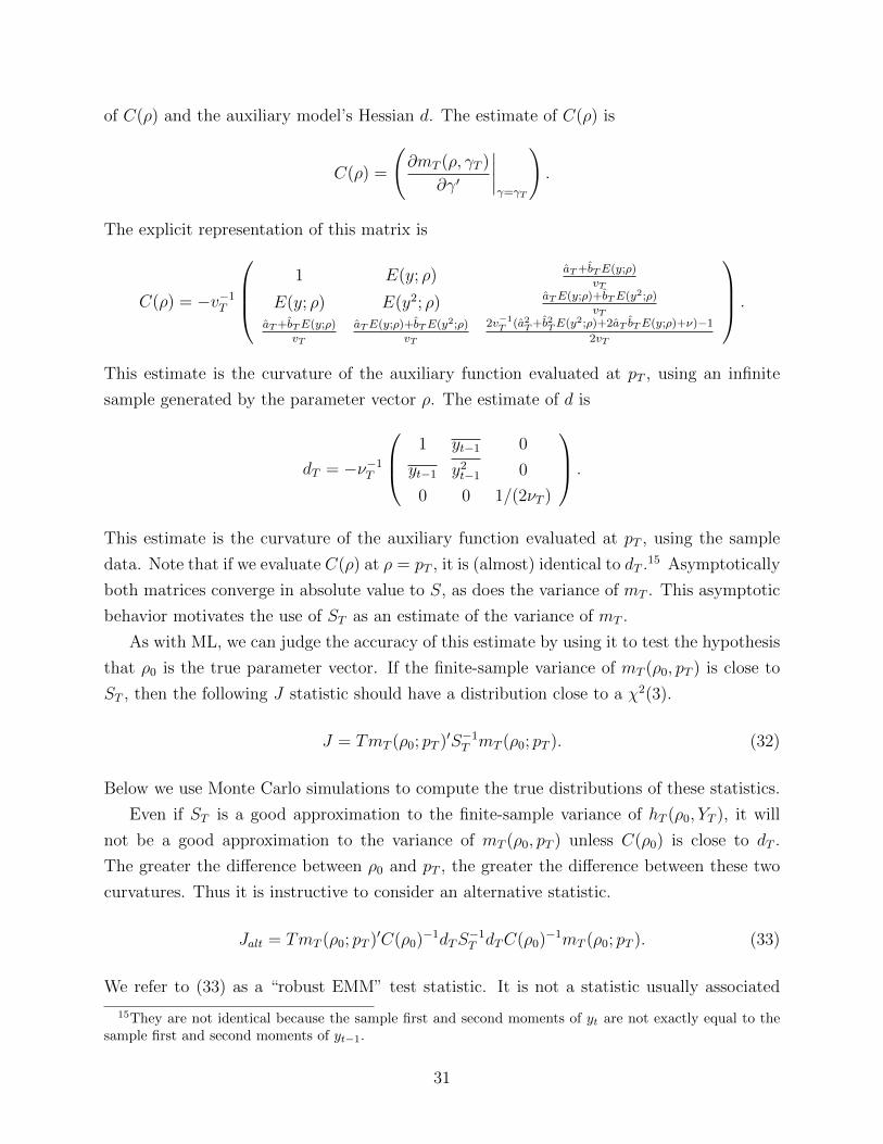
of C(ρ) and the auxiliary model’s Hessian d. The estimate of C(ρ) is

C(ρ) =

(∂mT (ρ, γT )

∂γ′

∣∣∣∣γ=γT

).

The explicit representation of this matrix is

C(ρ) = −v−1T

1 E(y; ρ) aT+bTE(y;ρ)

vT

E(y; ρ) E(y2; ρ) aTE(y;ρ)+bTE(y2;ρ)vT

aT+bTE(y;ρ)vT

aTE(y;ρ)+bTE(y2;ρ)vT

2v−1T (a2T+b2TE(y2;ρ)+2aT bTE(y;ρ)+ν)−1

2vT

.

This estimate is the curvature of the auxiliary function evaluated at pT , using an infinite

sample generated by the parameter vector ρ. The estimate of d is

dT = −ν−1T

1 yt−1 0

yt−1 y2t−1 0

0 0 1/(2νT )

.

This estimate is the curvature of the auxiliary function evaluated at pT , using the sample

data. Note that if we evaluate C(ρ) at ρ = pT , it is (almost) identical to dT .15 Asymptotically

both matrices converge in absolute value to S, as does the variance of mT . This asymptotic

behavior motivates the use of ST as an estimate of the variance of mT .

As with ML, we can judge the accuracy of this estimate by using it to test the hypothesis

that ρ0 is the true parameter vector. If the finite-sample variance of mT (ρ0, pT ) is close to

ST , then the following J statistic should have a distribution close to a χ2(3).

J = TmT (ρ0; pT )′S−1T mT (ρ0; pT ). (32)

Below we use Monte Carlo simulations to compute the true distributions of these statistics.

Even if ST is a good approximation to the finite-sample variance of hT (ρ0, YT ), it will

not be a good approximation to the variance of mT (ρ0, pT ) unless C(ρ0) is close to dT .

The greater the difference between ρ0 and pT , the greater the difference between these two

curvatures. Thus it is instructive to consider an alternative statistic.

Jalt = TmT (ρ0; pT )′C(ρ0)−1dTS

−1T dTC(ρ0)

−1mT (ρ0; pT ). (33)

We refer to (33) as a “robust EMM” test statistic. It is not a statistic usually associated

15They are not identical because the sample first and second moments of yt are not exactly equal to thesample first and second moments of yt−1.

31

with EMM because it relies on the ability to compute C(ρ). We can compute it analytically

in this simple case, but when the true likelihood function is unknown or intractable this

matrix is also either unknown or intractable.

8.3 Monte Carlo Results

We use Monte Carlo simulations to study the finite-sample properties of these estimation

techniques. We set α0 = 0 and ν0 = 1, and focus on values of β0 that are very close to

one. Given ρ0, we use the AR model to simulate a set of data YT . We then calculate the

ML estimate ρT , the estimated asymptotic variance of the moments ST , the GMM moment

vector hT (ρ0, YT ), and the EMM moment vector mT (ρ0, pT ). We also calculate the tests of

the true model (30), (32), and (33).

We summarize the behavior of the simulated ML and EMM moment vectors with their

sample variances across the Monte Carlo simulations. We then compare these empirical

variances to the mean, across the simulations, of ST . The results are displayed in Table 10.

To simplify the interpretation of the results, the empirical variances of the individual elements

of these moment vectors are divided by the mean of the corresponding diagonal elements

of ST . To conserve space the table does not report the ratio of the variance of the EMM

moment vector to the more robust estimate of its variance, C(ρ0)d−1T STd

−1T C(ρ0). We discuss

this ratio in the text.

The first two rows of the table consider the case of β0 = 0.99875, which is the AR(1)

coefficient for weekly observations of the instantaneous interest rate from a Vasicek model

with a speed of mean reversion of 0.065. With 1000 observations (the first row), the mean

estimate of β is biased down. If the data are weekly, the annual speed of mean reversion

implied by this mean coefficient is 0.11.

Although the estimate of β is biased, the finite-sample variance of the ML moment is close

to its estimated asymptotic value. The ratios of individual variances lie between 0.98 and

1.1. By contrast, the finite-sample variance of the EMM moment vector differ dramatically

from its estimated asymptotic value. The ratios of individual variances range from 0.01 to 12.

The main reason for this large divergence between finite-sample and estimated asymptotic

behavior is that the curvature of the likelihood function in the neighborhood of truth differs

from the curvature in the neighborhood of the ML estimates. The robust estimate of the

variance of the EMM moment vector corrects for this difference in curvature. With this

correction, the ratios of the empirical variances of the elements of the EMM moment vector

to the corresponding diagonal elements of this robust variance estimate (not reported in the

table) range from 1.12 to 2.20.

32

Given these results concerning the accuracy of the asymptotic variance estimates, it is

not surprising that the EMM test (32) of the hypothesis ρ = ρ0 is rejected at the five percent

asymptotic level in roughly three-quarters of the simulations. The ML test also over-rejects

truth, but the empirical rejection rate at the five percent level is a more modest eight percent.

The robust EMM test rejects the hypothesis ρ = ρ0 in twelve percent of the simulations.

Doubling the amount of data reduces the difference between the ML and EMM results, but

as the second row of the table shows, the behavior of the EMM moment vector still differs

substantially from its asymptotic behavior.

The third and fourth rows of the table reports results for a less persistent process: β0 =

0.95. For weekly data, this corresponds to speed of mean reversion of 2.67. The lower

persistence produces finite-sample behavior of the EMM moment vector that is much closer

to its asymptotic behavior. For example, with 1000 observations, the ratios of true variances

of the three EMM moments to their estimated asymptotic variances range from 0.96 to 1.13.

Nonetheless, with 1000 observations the true model is over-rejected; the rejection rate is

thirteen percent using the five percent asymptotic test statistic.

Zhou (2001) also shows that EMM over-rejects the true model when the data exhibit high

persistence. He simulates a square-root diffusion model of the instantaneous interest rate and

calls the empirical rejection rate with EMM/SNP “unacceptably large.” Our contribution

is to explain the source of this behavior. It is a consequence of the fact that when the data

are highly persistent, the curvature of the log-likelihood function evaluated using the sample

data diverges from the curvature evaluated using the true parameters. More generally,

convergence of the variability of the EMM moment vector to the variability of the auxiliary

score vector requires longer samples of data than are usually available to the econometrician.

In practice, we are seldom confronted with a problem in which the divergence between

the curvature of f using the sample data and the curvature using data generated by the

true model is relevant: we usually do not know the true model. But the main message here

carries over to a much broader class of problems. Anytime there is a divergence between

the properties of the sample data and the simulated data, there will also be a divergence

in the curvature of the log-likelihood function. This situation arises whenever the number

of moment conditions exceeds the number of free parameters. In this case, the moments

cannot be set exactly to zero, and instead a quadratic form in those moments is minimized

(see Equation (8)). The moments are weighted by the inverse of their estimated asymptotic

variance. If this matrix differs substantially from the true variance of the EMM moment

vector, it will result in both inefficient parameter estimates and incorrect statistical inference.

As the results in this paper have shown, this is a particular problem in a term structure

setting when SNP is used as the auxiliary model. When panel data are used to estimate the

33

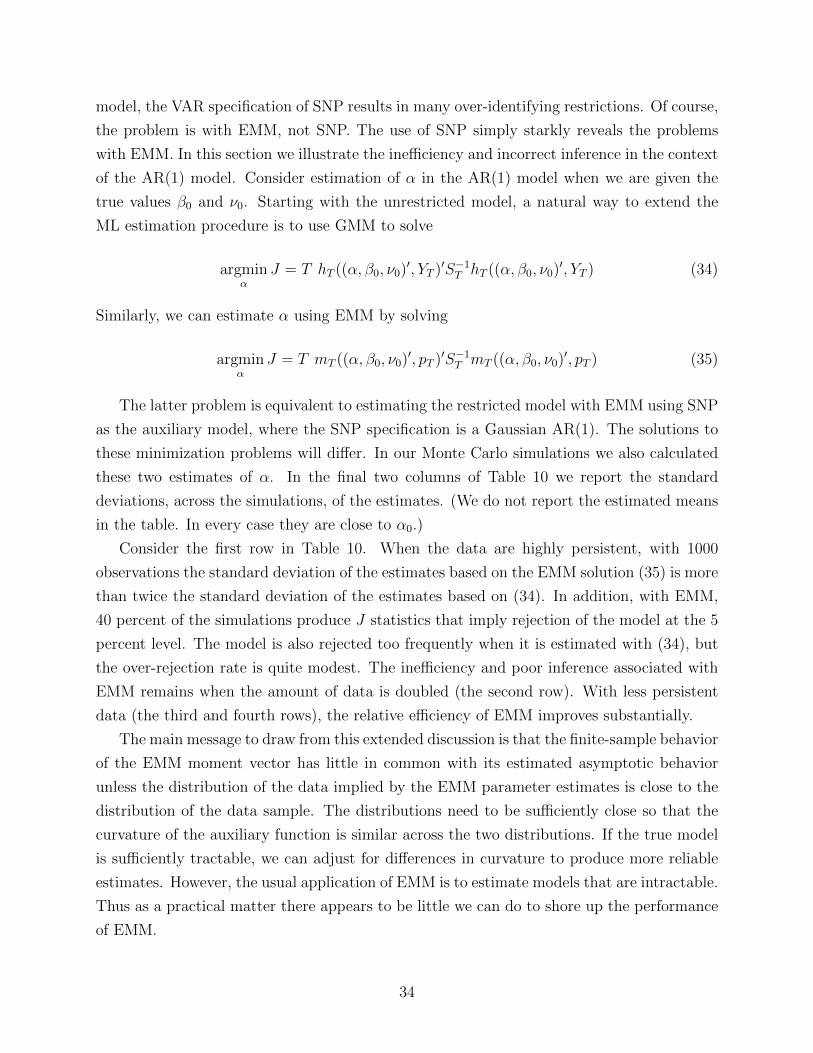
model, the VAR specification of SNP results in many over-identifying restrictions. Of course,

the problem is with EMM, not SNP. The use of SNP simply starkly reveals the problems

with EMM. In this section we illustrate the inefficiency and incorrect inference in the context

of the AR(1) model. Consider estimation of α in the AR(1) model when we are given the

true values β0 and ν0. Starting with the unrestricted model, a natural way to extend the

ML estimation procedure is to use GMM to solve

argminα

J = T hT ((α, β0, ν0)′, YT )′S−1T hT ((α, β0, ν0)

′, YT ) (34)

Similarly, we can estimate α using EMM by solving

argminα

J = T mT ((α, β0, ν0)′, pT )′S−1T mT ((α, β0, ν0)

′, pT ) (35)

The latter problem is equivalent to estimating the restricted model with EMM using SNP

as the auxiliary model, where the SNP specification is a Gaussian AR(1). The solutions to

these minimization problems will differ. In our Monte Carlo simulations we also calculated

these two estimates of α. In the final two columns of Table 10 we report the standard

deviations, across the simulations, of the estimates. (We do not report the estimated means

in the table. In every case they are close to α0.)

Consider the first row in Table 10. When the data are highly persistent, with 1000

observations the standard deviation of the estimates based on the EMM solution (35) is more

than twice the standard deviation of the estimates based on (34). In addition, with EMM,

40 percent of the simulations produce J statistics that imply rejection of the model at the 5

percent level. The model is also rejected too frequently when it is estimated with (34), but

the over-rejection rate is quite modest. The inefficiency and poor inference associated with

EMM remains when the amount of data is doubled (the second row). With less persistent

data (the third and fourth rows), the relative efficiency of EMM improves substantially.

The main message to draw from this extended discussion is that the finite-sample behavior

of the EMM moment vector has little in common with its estimated asymptotic behavior

unless the distribution of the data implied by the EMM parameter estimates is close to the

distribution of the data sample. The distributions need to be sufficiently close so that the

curvature of the auxiliary function is similar across the two distributions. If the true model

is sufficiently tractable, we can adjust for differences in curvature to produce more reliable

estimates. However, the usual application of EMM is to estimate models that are intractable.

Thus as a practical matter there appears to be little we can do to shore up the performance

of EMM.

34

9 Conclusions

The analysis in this paper leads to several important conclusions. First, despite its well-

known asymptotic optimality properties, maximum likelihood yields highly biased parameter

estimates in settings representative of those used in the estimation of modern term structure

models. This differs from the results of Ball and Torous (1996). They find that when

cross-sectional information is used in estimation, the bias in the estimated speed of mean

reversion and price of risk disappears. However, they only consider very simple forms for the

market price of interest rate risk. Their conclusion does not hold when we allow the price

of risk to be more flexible, such as the forms specified by Duarte (2004) and Duffee (2002).

Once the physical and equivalent-martingale drifts are decoupled, the use of cross-sectional

information can no longer eliminate the time-series related bias in the estimated speed of

mean reversion.

Our second conclusion is that, despite its asymptotic equivalence to maximum likelihood,

the Efficient Method of Moments is an unacceptable alternative to maximum likelihood in

finite samples. Most surprisingly, this is true even in settings where maximum likelihood

performs well. Much larger samples are required for the small-sample performance of EMM

to approach its asymptotic behavior than is the case for ML.

Our third conclusion is that the Kalman filter is a reasonable alternative to maximum

likelihood, even in non-Gaussian settings where the two are not equivalent. Unsurprisingly,

when feasible, ML usually makes more efficient use of the information in the sample than

does the Kalman filter, but the Kalman filter is vastly superior to EMM.

These results underscore the importance of performing detailed Monte Carlo analysis to

study the small-sample properties of new estimators, rather than merely relying on their

asymptotic properties. As we have shown in this paper, even techniques that are asymptot-

ically equivalent can have very different properties when used on finite samples.

35

A SNP as the Auxiliary Model for EMM

The standard auxiliary model for use with EMM has become the SNP (for SemiNonParametric)

model of Gallant and Tauchen (1992) (see also the user’s guide, Gallant and Tauchen, 1998).

It consists of writing the conditional density of the dataset under analysis in the form of a

Hermite polynomial multiplied by a normal density, i.e.,

f(yt | xt−1, ρ) = c(xt−1) [h(zt | xt−1)]2 φ(zt),

where

• φ(.) represents the standard normal p.d.f.,

• h(zt | xt−1) is a Hermite polynomial in zt,

• c(xt−1) is a normalization constant (equal to 1/∫

[h(s | xt−1)]2 φ(s) ds), and

• zt is a normalized version of yt, defined by

zt = R−1x,t−1 (yt − µx,t−1) ,

where µx,t−1 is the conditional mean, and R−1x,t−1 the Cholesky decomposition of the con-

ditional variance of yt. This specification allows great flexibility in fitting the conditional

distribution. In particular, we are free to choose:

• the dimensionality of the Hermite polynomial in z, Kz (allows for non-Gaussian be-

havior).

• the degree of the polynomial in x that makes up each of the coefficients in the Hermite

polynomial, Kx (another way to allow for conditional heterogeneity).

• the number of lags of x in the Hermite polynomial, Kp.

• the number of lags in a VAR specification for µx,t−1, Lµ.

• the degree of an ARCH (or GARCH, setting Lg > 0) specification for the scale trans-

formation Rx,t−1, Lr.

Choice of an appropriate specification is performed by using a model selection criterion, such

as the Schwarz Bayes information criterion (see Schwarz, 1978), which rewards good fit while

penalizing over-parametrization. Gallant and Tauchen (1998) discuss a search strategy for

finding an appropriate parametrization for a given problem.

36

References

Ahn, Dong-Hyun, Robert F. Dittmar, and A. Ronald Gallant, 2002, Quadratic term struc-

ture models: Theory and evidence, Review of Financial Studies 16, 459–485.

Ahn, Dong-Hyun, and Bin Gao, 1999, A parametric nonlinear model of term structure

dynamics, Review of Financial Studies 12, 721–762.

Aıt-Sahalia, Yacine, 1996, Testing continuous-time models of the spot interest rate, Review

of Financial Studies 9, 385–426.

Aıt-Sahalia, Yacine, 1999, Transition densities for interest rate and other diffusions, Journal

of Finance 54, 1361–1395.

Aıt-Sahalia, Yacine, 2008, Closed-form likelihood expansions for multivariate diffusions, An-

nals of Statistics 36, 906–937.

Aıt-Sahalia, Yacine, and Robert Kimmel, 2010, Estimating affine multifactor term structure

models using closed-form likelihood expansions, Journal of Financial Economics 98, 113–

144.

Andersen, Torben G., Hyung-Jin Chung, and Bent E. Sørensen, 1999, Efficient method of

moments estimation of a stochastic volatility model: A Monte Carlo study, Journal of

Econometrics 91, 61–87.

Andersen, Torben G., and Jesper Lund, 1997, Estimating continuous time stochastic volatil-

ity models of the short term interest rate, Journal of Econometrics 77, 343–377.

Andersen, Torben G., and Bent E. Sørensen, 1996, GMM estimation of a stochastic volatility

model: A Monte Carlo study, Journal of Business and Economic Statistics 14, 328–352.

Backus, David K., Silverio Foresi, Abon Mozumdar, and Liuren Wu, 2001, Predictable

changes in yields and forward rates, Journal of Financial Economics 59, 281–311.

Ball, Clifford A., and Walter N. Torous, 1996, Unit roots and the estimation of interest rate

dynamics, Journal of Empirical Finance 3, 215–238.

Bates, David S., 2006, Maximum likelihood estimation of latent affine processes, Review of

Financial Studies 19, 909–965.

Beaglehole, David, and Mark Tenney, 1992, A nonlinear equilibrium model of the term

structure of interest rates: Corrections and additions, Journal of Financial Economics 32,

345–354.

37

Boudoukh, Jacob, Chris Downing, Matthew Richardson, Richard Stanton, and Robert F.

Whitelaw, 2010, A multifactor, nonlinear, continuous-time model of interest rate volatility,

in Tim Bollerslev, Jeffrey R. Russell, and Mark W. Watson, eds., Volatility and Time

Series Econometrics: Essays in Honor of Robert F. Engle, chapter 14, 296–322 (Oxford

University Press, Oxford).

Brandt, Michael W., and Ping He, 2002, Simulated likelihood estimation of affine term

structure models from panel data, Working paper, University of Pennsylvania.

Brandt, Michael W., and Pedro Santa-Clara, 2002, Simulated likelihood estimation of dif-

fusions with an application to exchange rate dynamics in incomplete markets, Journal of

Financial Economics 63, 161–210.

Campbell, John Y., and Robert J. Shiller, 1991, Yield spreads and interest rate movements:

A bird’s eye view, Review of Economic Studies 58, 495–514.

Chen, Ren-Raw, and Louis Scott, 1993, Maximum likelihood estimation for a multifactor

equilibrium model of the term structure of interest rates, Journal of Fixed Income 3,

14–31.

Chen, Ren-Raw, and Louis Scott, 2003, Multifactor Cox-Ingersoll-Ross models of the term

structure: Estimates and tests from a Kalman filter model, Journal of Real Estate Finance

and Economics 27, 143–172.

Chumacero, Romulo A., 1997, Finite sample properties of the efficient method of moments,

Studies in Nonlinear Dynamics and Econometrics 2, 35–51.

Conley, Timothy G., Lars Peter Hansen, Erzo G. J. Luttmer, and Jose A. Scheinkman,

1997, Short-term interest rates as subordinated diffusions, Review of Financial Studies

10, 525–577.

Constantinides, George M., 1992, A theory of the nominal term structure of interest rates,

Review of Financial Studies 5, 531–552.

Cox, John C., Jonathan E. Ingersoll, Jr., and Stephen A. Ross, 1985, A theory of the term

structure of interest rates, Econometrica 53, 385–407.

Dai, Qiang, and Kenneth J. Singleton, 2000, Specification analysis of affine term structure

models, Journal of Finance 55, 1943–1978.

de Jong, Frank, 2000, Time-series and cross-section information in affine term structure

models, Journal of Business and Economic Statistics 18, 300–314.

38

Duan, Jin-Chuan, and Jean-Guy Simonato, 1999, Estimating and testing exponential-affine

term structure models by Kalman filter, Review of Quantitative Finance and Accounting

13, 111–135.

Duarte, Jefferson, 2004, Evaluating an alternative risk preference in affine term structure

models, Review of Financial Studies 17, 379–404.

Duffee, Gregory R., 2002, Term premia and interest rate forecasts in affine models, Journal

of Finance 57, 405–443.

Duffee, Gregory R., and Richard Stanton, 2008, Evidence on simulation inference for near

unit-root processes with implications for term structure estimation, Journal of Financial

Econometrics 6, 108–142.

Duffie, Darrell, and Rui Kan, 1996, A yield-factor model of interest rates, Mathematical

Finance 6, 379–406.

Duffie, Darrell, and Kenneth J. Singleton, 1993, Simulated moments estimation of Markov

models of asset prices, Econometrica 61, 929–952.

Ferson, Wayne E., and Stephen R. Foerster, 1994, Finite sample properties of the Generalized

Method of Moments in tests of conditional asset pricing models, Journal of Financial

Economics 36, 29–55.

Gallant, A. Ronald, and Jonathan R. Long, 1997, Estimating stochastic differential equations

efficiently by minimum chi-square, Biometrika 84, 125–141.

Gallant, A. Ronald, and George Tauchen, 1997, Estimation of continuous-time models for

stock returns and interest rates, Macroeconomic Dynamics 1, 135–168.

Gallant, A. Ronald, and George E. Tauchen, 1992, A nonparametric approach to nonlinear

time series analysis: Estimation and simulation, in David Brillinger, Peter Caines, John

Geweke, Emanuel Parzen, Murray Rosenblatt, and Murad S. Taqqu, eds., New Directions

in Time Series Analysis, Part II , 71–92 (Springer-Verlag, New York, NY).

Gallant, A. Ronald, and George E. Tauchen, 1996, Which moments to match?, Econometric

Theory 12, 657–681.

Gallant, A. Ronald, and George E. Tauchen, 1998, SNP: A program for nonparametric time

series analysis, version 8.7, User’s guide, University of North Carolina, Chapel Hill.

39

Geyer, Alois L. J., and Stefan Pichler, 1999, A state-space approach to estimate and test

multifactor Cox-Ingersoll-Ross models of the term structure, Journal of Financial Research

22, 107–130.

Hansen, Lars Peter, John C. Heaton, and Amir Yaron, 1996, Finite-sample properties of some

alternative GMM estimators, Journal of Business and Economic Statistics 14, 262–280.

Jegadeesh, Narasimhan, and George G. Pennacchi, 1996, The behavior of interest rates

implied by the term structure of Eurodollar futures, Journal of Money, Credit and Banking

28, 426–446.

Kitagawa, Genshiro, 1987, Non-Gaussian state-space modeling of nonstationary time series,

Journal of the American Statistical Association 82, 1032–1041.

Kloeden, Peter E., and Eckhard Platen, 1992, Numerical Solution of Stochastic Differential

Equations (Springer-Verlag, New York, NY).

Kocherlakota, Narayana R., 1990, On tests of representative consumer asset pricing models,

Journal of Monetary Economics 26, 285–304.

Kohn, Robert, and Craig F. Ansley, 1987, Comment, Journal of the American Statistical

Association 82, 1041–1044.

Leippold, Markus, and Liuren Wu, 2002, Asset pricing under the quadratic class, Journal of

Financial and Quantitative Analysis 37, 271–295.

Lo, Andrew W., 1988, Maximum likelihood estimation of generalized Ito processes with

discretely sampled data, Econometric Theory 4, 231–247.

Longstaff, Francis A., 1989, A nonlinear general equilibrium model of the term structure,

Journal of Financial Economics 23, 195–224.

Lu, Biao, 1999, A maximum-likelihood estimation of the Constantinides and Cox, Ingersoll,

and Ross models of the term structure of interest rates, Working paper, University of

Michigan.

Lund, Jesper, 1997, Non-linear Kalman filtering techniques for term structure models, Work-

ing paper, Aarhus School of Business.

Martin, R. Douglas, and Adrian E. Raftery, 1987, Comment: Robustness, computation, and

non-Euclidean models, Journal of the American Statistical Association 82, 1044–1050.

40

Øksendal, Bernt, 2002, Stochastic Differential Equations: An Introduction with Applications ,

fifth edition (Springer-Verlag, New York, NY).

Pearson, Neil D., and Tong-Sheng Sun, 1994, Exploiting the conditional density in estimating

the term structure: An application to the Cox, Ingersoll, and Ross model, Journal of

Finance 49, 1279–1304.

Pedersen, Asger Roer, 1995, A new approach to maximum likelihood estimation of stochastic

differential equations based on discrete observations, Scandinavian Journal of Statistics

22, 55–71.

Pennacchi, George G., 1991, Identifying the dynamics of real interest rates and inflation:

Evidence using survey data, Review of Financial Studies 4, 53–86.

Pfann, Gerard A., Peter C. Schotman, and Rolf Tschernig, 1996, Nonlinear interest rate

dynamics and implications for the term structure, Journal of Econometrics 74, 149–176.

Santa-Clara, Pedro, 1995, Simulated likelihood estimation of diffusions with an application

to the short term interest rate, Working paper, INSEAD.

Schwarz, Gideon, 1978, Estimating the dimension of a model, Annals of Statistics 6, 461–464.

Stanton, Richard, 1997, A nonparametric model of term structure dynamics and the market

price of interest rate risk, Journal of Finance 52, 1973–2002.

Tauchen, George E., 1986, Statistical properties of generalized method-of-moments estima-

tors of structural parameters obtained from financial market data, Journal of Business

and Economic Statistics 4, 397–416.

Vasicek, Oldrich A., 1977, An equilibrium characterization of the term structure, Journal of

Financial Economics 5, 177–188.

Zhou, Hao, 2001, Finite sample properties of EMM, GMM, QMLE, and MLE for a square-

root interest rate diffusion model, Journal of Computational Finance 5, 89–122.

41

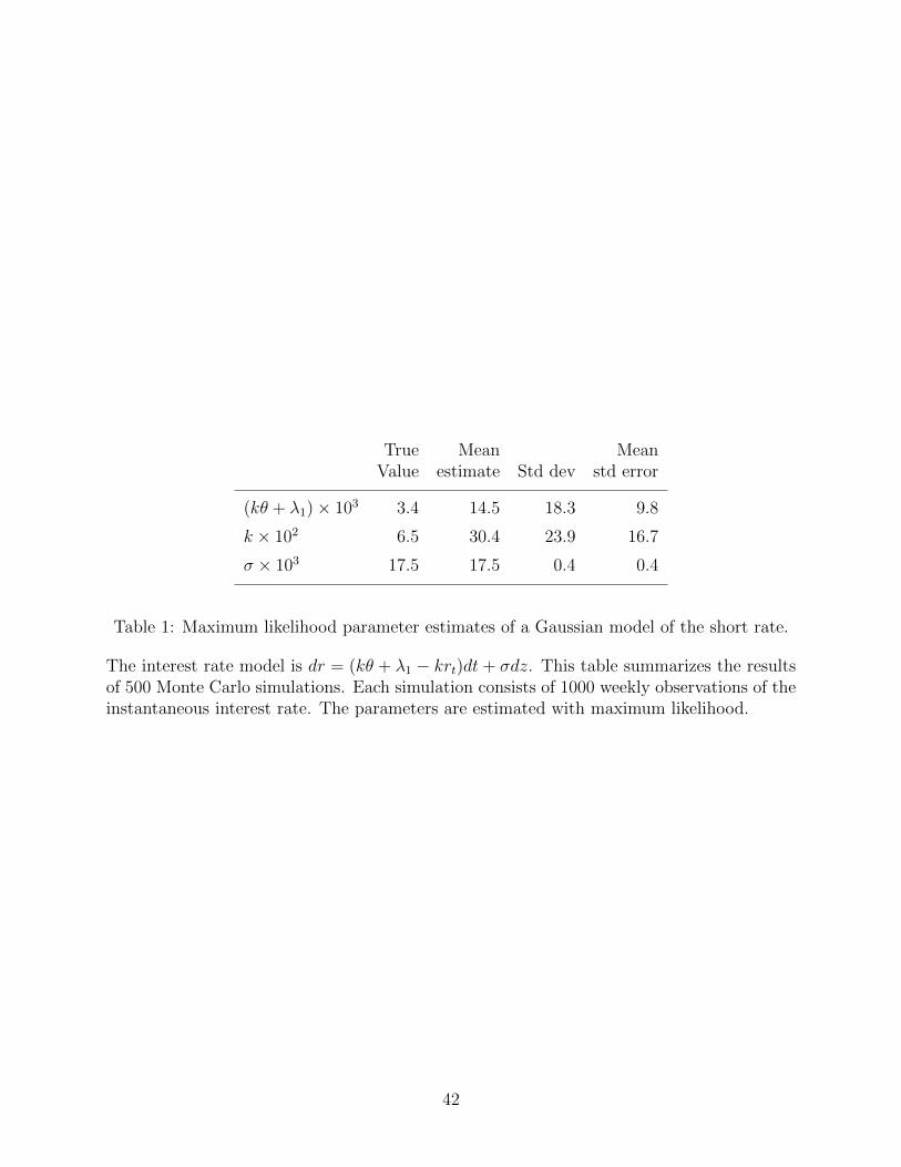
True Mean MeanValue estimate Std dev std error

(kθ + λ1)× 103 3.4 14.5 18.3 9.8

k × 102 6.5 30.4 23.9 16.7

σ × 103 17.5 17.5 0.4 0.4

Table 1: Maximum likelihood parameter estimates of a Gaussian model of the short rate.

The interest rate model is dr = (kθ + λ1 − krt)dt+ σdz. This table summarizes the resultsof 500 Monte Carlo simulations. Each simulation consists of 1000 weekly observations of theinstantaneous interest rate. The parameters are estimated with maximum likelihood.

42

Kalman filter (ML) EMM/SNPTrue Std Mean Std Mean

Parameter Value Mean dev std err Mean dev std err

kθ × 103 8.4 8.4 0.24 0.23 8.0 0.34 0.20

k × 102 6.5 6.5 0.31 0.31 6.5 0.31 0.25

σ × 103 17.5 17.5 1.02 0.99 12.2 3.76 1.23

λ1 × 103 −5.0 −5.0 2.33 3.35 −4.2 2.55 0.66√V × 103 6.0 6.0 0.09 0.09 6.0 0.11 0.08

Table 2: Parameter estimates of a one-factor Gaussian model with constant price of risk

The model is given by equations (19) and (20) in the text, with λ2 = 0. This table summarizesthe results of 500 Monte Carlo simulations. With each simulation, 1000 weeks of yieldson bonds with maturities of three months, one year, and ten years are observed with iidmeasurement error. The standard deviation of the error is

√V . The parameters of the

model are estimated with the Kalman filter (which is ML) and with EMM/SNP. The meannumber of overidentifying moments with EMM/SNP is 23.6. The EMM χ2 test rejects themodel at the 5% level in 43.2% of the simulations and rejects at the 1% level in 28.6% of thesimulations.

43

Kalman filter (ML) EMM/SNPTrue Std Mean Std Mean

Parameter Value Mean dev std err Mean dev std err

kθ × 103 8.4 8.4 0.31 0.30 8.4 0.47 0.37

k × 102 6.5 6.5 0.39 0.37 6.5 0.60 0.45

σ × 103 17.5 17.7 1.04 1.02 12.2 1.58 1.57

λ1 × 103 5.0 20.0 16.98 14.12 25.0 46.78 17.33

λ2 × 102 −14.0 −37.4 24.14 20.96 −43.7 53.37 25.06√V × 103 6.0 6.0 0.09 0.09 6.0 0.10 0.09

Table 3: Parameter estimates of a one-factor Gaussian model with affine price of risk

The model is given by equations (19) and (20) in the text. This table summarizes the resultsof 500 Monte Carlo simulations. With each simulation, 1000 weeks of yields on bonds withmaturities of three months, one year, and ten years are observed with iid measurement error.The standard deviation of the error is

√V . The parameters of the model are estimated with

the Kalman filter (which is ML) and with EMM/SNP. The mean number of overidentifyingmoments with EMM/SNP is 22.5. The EMM χ2 test rejects the model at the 5% level in5.6% of the simulations and rejects at the 1% level in 1.4% of the simulations.

44

5b

onds

2b

onds

10b.p

.m

easu

rem

ent

erro

rT

rue

Std

Mea

nStd

Mea

nStd

Mea

nP

aram

eter

Val

ue

Mea

ndev

std

err

Mea

ndev

std

err

Mea

ndev

std

err

kθ×

103

8.4

8.4

0.27

0.26

8.4

0.34

0.32

8.4

0.06

0.06

k×

102

6.5

6.5

0.34

0.33

6.5

0.41

0.39

6.5

0.06

0.06

σ×

103

17.5

17.6

0.83

0.83

17.6

1.22

1.19

17.5

0.42

0.43

λ1×

103

5.0

19.8

16.7

413

.95

20.0

16.9

214

.22

19.5

16.2

413

.73

λ2×

102

−14.0−

37.0

23.5

020

.67−

37.3

24.1

321

.12−

36.7

23.0

420

.29

√V×

103

Var

ies

6.0

0.07

0.06

6.0

0.11

0.11

1.0

0.02

0.02

Tab

le4:

Max

imum

like

lihood

par

amet

eres

tim

ates

ofa

one-

fact

orG

auss

ian

model

wit

haffi

ne

pri

ceof

risk

:va

ryin

gas

sum

pti

ons

The

model

isgi

ven

by

equat

ions

(19)

and

(20)

inth

ete

xt.

This

table

sum

mar

izes

the

resu

lts

ofth

ree

sets

of50

0M

onte

Car

losi

mula

tion

s.W

ith

each

sim

ula

tion

,10

00w

eeks

ofyie

lds

onb

onds

wit

hm

aturi

ties

ofra

ngi

ng

from

thre

em

onth

sto

ten

year

sar

eob

serv

edw

ith

iid

mea

sure

men

ter

ror.

The

stan

dar

ddev

iati

onof

the

erro

ris√V

,se

tto

60bas

isp

oints

inth

efirs

ttw

ose

tsof

sim

ula

tion

san

d10

bas

isp

oints

inth

eth

ird

set.

The

thir

dse

tal

soas

sum

esth

atth

ree

bon

dyie

lds

are

obse

rved

.

45

Panel A. Weekly observations

500 obs 2000 obsTrue Std Mean Std Mean

Parameter Value Mean dev std err Mean dev std err

kθ × 103 8.4 8.5 0.57 0.53 8.4 0.19 0.19

k × 102 6.5 6.5 0.71 0.66 6.5 0.23 0.22

σ × 103 17.5 17.7 1.37 1.48 17.6 0.70 0.71

λ1 × 103 5.0 36.9 34.99 25.57 12.4 10.27 8.70

λ2 × 102 −14.0 −62.7 48.44 38.03 −25.6 15.10 12.70√V × 103 6.0 6.0 0.12 0.12 6.0 0.06 0.06

Panel B. Monthly observations

240 obs 480 obsTrue Std Mean Std Mean

Parameter Value Mean dev std err Mean dev std err

kθ × 103 8.4 8.4 0.67 0.61 8.4 0.37 0.37

k × 102 6.5 6.5 0.82 0.77 6.5 0.47 0.46

σ × 103 17.5 17.7 1.52 1.50 17.6 0.99 1.03

λ1 × 103 5.0 20.2 20.25 14.63 12.2 9.95 8.71

λ2 × 102 −14.0 −37.3 26.94 21.75 −25.2 13.95 12.83√V × 103 6.0 6.0 0.20 0.19 6.0 0.13 0.13

Table 5: Maximum likelihood parameter estimates of a one-factor Gaussian model with affineprice of risk: varying assumptions

The model is given by equations (19) and (20) in the text. This table summarizes the resultsof four sets of 500 Monte Carlo simulations. With each simulation, yields on bonds withmaturities of ranging from three months to ten years are observed with iid measurementerror. The standard deviation of the error is

√V .

46

Exac

tM

LK

alm

an

filt

erE

MM

/S

NP

Tru

eS

tdM

ean

Med

ian

Std

Mea

nM

edia

nS

tdM

ean

Med

ian

Par

amet

erV

alu

eM

ean

Med

ian

dev

std

err

std

err

Mea

nM

edia

nd

evst

der

rst

der

rM

ean

Med

ian

dev

std

err

std

err

δ 0×

102

1.0

1.0

1.0

0.67

0.2

80.2

30.6

1.2

2.8

31.9

10.9

4−

32.8

2.7

190.7

0265.7

51.7

6

kθ×

103

7.5

7.5

7.5

0.56

0.2

70.2

37.8

7.4

2.2

71.5

90.7

934.2

5.8

154.1

2209.5

11.4

6

k×

102

6.3

6.3

6.3

0.26

0.2

10.2

06.3

6.2

0.6

70.6

20.5

94.2

4.7

3.0

82.7

32.0

7

σ×

102

8.0

8.0

8.1

0.44

0.2

80.2

88.1

8.1

1.2

31.0

60.9

79.6

10.1

5.0

73.8

33.5

7

λ2×

102

−6.8

−9.

2−

7.6

7.04

2.2

31.7

7−

11.2

−9.5

8.7

17.5

27.0

6−

19.

4−

13.5

22.4

225.8

69.0

5√V×

103

Var

ies

7.0

7.0

0.11

0.1

10.1

16.0

6.0

0.0

90.0

90.0

95.9

5.9

0.3

20.0

90.0

9

Tab

le6:

Par

amet

eres

tim

ates

ofa

one-

fact

orsq

uar

e-ro

otm

odel

wit

hlinea

rri

skpre

miu

m

The

model

isgi

ven

by

equat

ions

(21)

thro

ugh

(23)

inth

ete

xt,

wit

hλ1

=0.

This

table

sum

mar

izes

the

resu

lts

of50

0M

onte

Car

losi

mula

tion

s.W

ith

each

sim

ula

tion

,10

00w

eeks

ofyie

lds

onth

ree

bon

ds

wit

hm

aturi

ties

rangi

ng

from

thre

em

onth

s,on

eye

ar,

and

ten

year

sar

eob

serv

ed.

For

“Exac

tM

L”,

the

ten-y

ear

yie

ldis

obse

rved

wit

hou

ter

ror

and

the

thre

e-m

onth

and

one-

year

yie

lds

are

obse

rved

wit

hnor

mal

lydis

trib

ute

d,

iid

mea

sure

men

ter

ror.

The

stan

dar

ddev

iati

onof

the

erro

r,√V

,is

70bas

isp

oints

.F

orK

alm

anfilt

eres

tim

atio

nan

dE

MM

/SN

Pes

tim

atio

n,

all

thre

eyie

lds

are

obse

rved

wit

hm

easu

rem

ent

erro

r.T

he

stan

dar

ddev

iati

onof

the

erro

ris

60bas

isp

oints

.T

he

mea

nnum

ber

ofov

erid

enti

fyin

gre

stri

ctio

ns

wit

hE

MM

/SN

Pis

23.0

.T

he

EM

Mχ2

test

reje

cts

the

model

atth

efive

per

cent

leve

lin

26.4

per

cent

ofth

esi

mula

tion

san

dat

the

one

per

cent

leve

lin

17.4

per

cent

ofth

esi

mula

tion

s.

47

Sim

ula

ted

ML

Lin

eari

zed

Kalm

an

filt

erE

MM

/S

NP

Tru

eS

tdM

ean

Med

ian

Std

Mea

nM

edia

nS

tdM

ean

Med

ian

Par

amet

erV

alu

eM

ean

Med

ian

dev

std

err

std

err

Mea

nM

edia

nd

evst

der

rst

der

rM

ean

Med

ian

dev

std

err

std

err

δ 0×

102

1.0

1.0

1.0

0.61

0.4

90.3

40.5

1.1

3.1

22.2

41.0

0−

12.7

1.2

33.5

532.2

214.2

2

kθ×

103

7.5

7.5

7.5

0.51

0.4

40.3

37.9

7.5

2.5

01.8

50.8

718.4

7.4

27.3

025.1

111.5

2

k×

102

6.3

6.3

6.3

0.27

0.2

80.2

66.3

6.2

0.6

80.6

30.6

05.5

6.3

2.6

53.5

33.4

4

σ×

102

8.0

8.0

8.1

0.44

0.4

20.3

98.0

8.0

1.2

71.1

21.0

28.2

7.9

4.3

07.4

66.5

5

λ1×

102

0.0

11.1

8.5

11.0

59.0

28.4

010.3

7.2

13.2

09.9

18.3

530.7

9.4

145.7

775.1

720.5

4

λ2×

102

−6.8−

56.7

−46.3

46.8

139.6

437.9

9−

48.7

−37.9

45.0

737.9

335.9

1−

91.2

−41.

9435.6

579.0

940.6

5√V×

103

Var

ies

7.0

7.0

0.11

0.1

10.1

16.0

6.0

0.0

90.0

90.0

95.9

5.9

0.1

00.0

90.0

9

Tab

le7:

Par

amet

ers

esti

mat

esof

aon

e-fa

ctor

squar

e-ro

otm

odel

that

allo

ws

for

anon

linea

rri

skpre

miu

m

The

model

isgi

ven

by

equat

ions

(21)

thro

ugh

(23)

inth

ete

xt.

This

table

sum

mar

izes

resu

lts

from

500

Mon

teC

arlo

sim

ula

tion

s.W

ith

each

sim

ula

tion

,10

00w

eeks

ofyie

lds

ofb

onds

wit

hm

aturi

ties

ofth

ree

mon

ths,

one

year

,an

dte

nye

ars

are

obse

rved

.T

he

true

model

has

alinea

rri

skpre

miu

m,

while

the

esti

mat

edm

odel

sal

low

for

anon

linea

rri

skpre

miu

m.

For

“Sim

ula

ted

ML

”,th

ete

n-y

ear

yie

ldis

obse

rved

wit

hou

ter

ror

and

the

thre

e-m

onth

and

one-

year

yie

lds

are

obse

rved

wit

hnor

mal

lydis

trib

ute

d,

iid

mea

sure

men

ter

ror.

The

stan

dar

ddev

iati

onof

the

erro

r,√V

,is

70bas

isp

oints

.F

orlinea

rize

dK

alm

anfilt

eres

tim

atio

nan

dE

MM

/SN

Pes

tim

atio

n,

all

thre

eyie

lds

are

obse

rved

wit

hm

easu

rem

ent

erro

rw

ith

ast

andar

ddev

iati

onof

60bas

isp

oints

.T

he

mea

nnum

ber

ofov

erid

enti

fyin

gre

stri

ctio

ns

wit

hSN

P/E

MM

is22

.T

he

EM

Mχ2

test

reje

cts

the

model

atth

e5%

leve

lin

9.4

per

cent

ofth

esi

mula

tion

san

dat

the

1%le

vel

in4.

0p

erce

nt

ofth

esi

mula

tion

s.

48

Kal

man

filt

er(e

xac

tM

L)

EM

M/S

NP

Tru

eStd

Mea

nM

edia

nStd

Mea

nM

edia

nP

aram

eter

Val

ue

Mea

nM

edia

ndev

std

err

std

err

Mea

nM

edia

ndev

std

err

std

err

δ 0×

101.

01.

11.

01.

050.

690.

081.

61.

15.

04>

103

0.12

k1×

102

70.0

70.4

70.4

3.09

3.04

2.98

70.4

70.0

5.19

3.94

3.48

k2×

102

2.7

2.7

2.7

0.64

0.63

0.63

2.7

2.6

1.44

1.14

0.92

σ1×

102

2.0

2.0

2.0

0.09

0.09

0.09

2.0

2.0

0.13

0.11

0.10

σ2×

102

1.3

1.3

1.3

0.07

0.07

0.07

1.3

1.3

0.11

0.09

0.08

λ11×

102

−1.

0−

1.4

−1.

30.

840.

700.

66−

2.2

−1.

83.

891.

010.

70

λ21×

102

−0.

4−

1.4

−0.

87.

845.

150.

62−

14.8

−1.

1968

.11

91.1

21.

06

λ12×

102

10.0−

15.2

−8.

834

.68

30.3

430

.04−

61.5

−37.7

149.

0645

.45

31.2

5

λ22×

102−

12.0−

33.6

−27.9

23.5

718

.96

18.2

7−

120.

6−

50.6

267.

3492

.04

25.0

9√V×

103

2.0

2.0

2.0

0.04

0.04

0.04

2.0

2.0

0.04

0.03

0.03

Tab

le8:

Par

amet

eres

tim

ates

ofa

two-

fact

orG

auss

ian

model

wit

haffi

ne

pri

ceof

risk

The

model

isgi

ven

by

equat

ions

(24)

thro

ugh

(26)

inth

ete

xt.

This

table

sum

mar

izes

the

resu

lts

of50

0M

onte

Car

losi

mula

tion

s.W

ith

each

sim

ula

tion

,10

00w

eeks

ofyie

lds

onth

ree

bon

ds

wit

hm

aturi

ties

ofth

ree

mon

ths,

one

year

,an

dte

nye

ars

are

obse

rved

wit

hiid

mea

sure

men

ter

ror.

The

stan

dar

ddev

iati

onof

the

erro

ris√V

.T

he

par

amet

ers

ofth

em

odel

are

esti

mat

edw

ith

the

Kal

man

filt

er(w

hic

his

ML

)an

dw

ith

EM

M/S

NP

.T

he

mea

nnum

ber

ofov

erid

enti

fyin

gre

stri

ctio

ns

wit

hSN

P/E

MM

is23

.1.

The

EM

Mχ2

test

reje

cts

the

model

atth

e5%

leve

lin

7.4

per

cent

ofth

esi

mula

tion

san

dat

the

1%le

vel

in3.

2p

erce

nt

ofth

esi

mula

tion

s.

49

Simulated ML Linearized Kalman filterTrue Std Mean Std Mean

Parameter Value Mean dev std err Mean dev std err

δ0 × 102 −3.6 −3.7 0.93 0.88 −5.3 9.72 15.96

kθ1 × 102 4.0 4.0 0.26 0.28 4.4 2.40 2.02

kθ2 × 102 0.3 0.3 0.04 0.04 0.4 0.42 0.52

k1 × 102 70.0 69.9 2.18 2.25 70.7 3.67 3.77

k2 × 102 3.0 3.0 0.40 0.41 3.0 0.93 0.87

σ1 × 102 8.9 9.0 0.49 0.54 8.8 1.41 1.28

σ2 × 102 5.2 5.2 0.32 0.36 5.1 0.97 0.91

λ11 × 102 −20.0 −14.3 10.65 11.44 −9.1 17.64 16.17

λ21 × 102 0.5 8.1 10.98 7.63 9.8 14.05 15.51

λ12 × 102 66.0 35.4 56.19 59.11 13.5 65.86 65.61

λ22 × 102 −5.0 −40.6 47.28 36.16 −46.5 48.13 35.62√V × 103 2.0 2.0 0.04 0.05 2.0 0.03 0.03

Table 9: Parameter estimates of a two-factor square-root model with nonlinear risk premium

The model is given by equations (27) through (29) in the text. This table summarizes theresults of 500 Monte Carlo simulations. With each simulation, 1000 weeks of yields on threebonds with maturities of three months, one year, and ten years are observed. For “SimulatedML”, the three-month and ten-year yields are observed without error and the one-year yieldis observed with normally distributed, iid measurement error. The standard deviation of theerror,

√V , is 20 basis points.

50

Em

pir

ical

5%Std

dev

ofre

stri

cted

Rat

ioof

true

var

toes

tim

ated

asym

pto

tic

var

reje

ctio

nfr

eqes

tim

ates

ofα

Num

Mea

nM

Lm

omen

tsE

MM

mom

ents

Rob

ust

[em

p5%

reje

ctfr

eq]

obs

(T)

β0

βT

αβ

να

βν

ML

EM

ME

MM

ML

EM

M

1000

0.99

875

0.99

794

0.97

71.

095

1.01

312

.192

0.01

21.

901

0.07

80.

732

0.11

60.

032

0.06

5[.07

4][.40

0]

2000

0.99

875

0.99

829

1.03

71.

077

1.00

95.

449

0.01

21.

388

0.07

00.

454

0.07

20.

023

0.03

4[.06

8][.22

6]

1000

0.95

000

0.94

702

0.97

71.

021

1.01

41.

133

0.96

01.

076

0.05

20.

130

0.06

00.

032

0.03

0[.05

8][.11

6]

2000

0.95

000

0.94

838

1.03

71.

011

1.00

91.

103

0.91

71.

036

0.05

20.

074

0.05

40.

023

0.02

3[.06

0][.06

6]

Tab

le10

:R

esult

sof

Mon

teC

arlo

sim

ula

tion

ofM

Lan

dE

MM

esti

mat

ion

ofan

AR

(1)

model

This

table

rep

orts

resu

lts

from

500

Mon

teC

arlo

sim

ula

tion

s.T

he

sim

ula

ted

model

is

xt

=α0

+β0xt−

1+ε t,

ε t∼N

(0,ν

0),

α0

=0,ν 0

=1

For

each

sim

ula

tion

asa

mple

ofle

ngt

hT

isge

ner

ated

and

the

par

amet

ers

are

esti

mat

edw

ith

bot

hM

L(u

sing

the

scor

eve

ctor

ofth

elike

lihood

funct

ion

asth

em

omen

tve

ctor

inG

MM

esti

mat

ion)

and

wit

hE

MM

(usi

ng

the

true

like

lihood

funct

ion

asth

eau

xilia

rylike

lihood

funct

ion).

The

asym

pto

tic

vari

ance

ofth

em

omen

tve

ctor

sis

also

esti

mat

ed,

and

the

ML

and

EM

Mm

omen

tve

ctor

sar

eca

lcula

ted

atth

em

odel

’str

ue

par

amet

ers.

The

table

rep

orts

the

vari

ance

s,ac

ross

the

sim

ula

tion

s,of

thes

em

omen

tsdiv

ided

by

the

corr

esp

ondin

gm

eans

(acr

oss

the

sim

ula

tion

s)of

the

esti

mat

edas

ym

pto

tic

vari

ance

sof

thes

em

omen

ts.

For

exam

ple

,a

valu

eof

10fo

rα

implies

that

the

empir

ical

vari

ance

ofth

epar

tial

der

ivat

ive

ofth

elike

lihood

funct

ion

wit

hre

spec

ttoα

is10

tim

esth

em

ean

esti

mat

edas

ym

pto

tic

vari

ance

.T

he

sam

em

omen

tve

ctor

san

des

tim

ated

asym

pto

tic

vari

ance

sar

euse

dto

const

ruct

LR

test

sof

the

hyp

othes

isth

atth

em

odel

’spar

amet

ers

equal

the

true

par

amet

ers.

The

table

rep

orts

the

freq

uen

cyw

ith

whic

hth

ehyp

othes

isis

reje

cted

atth

e5%

leve

l.In

addit

ion,

are

stri

cted

vers

ion

ofth

em

odel

ises

tim

ated

wher

eβ0

andν 0

are

know

nan

dα

isunknow

n.

Sta

ndar

ddev

iati

ons

ofth

ees

tim

ates

ofα

are

dis

pla

yed

inth

efinal

two

colu

mns

alon

gw

ith

the

freq

uen

cyw

ith

whic

hth

ehyp

othes

isth

atα

=α0

isre

ject

edat

the

5%le

vel.

51

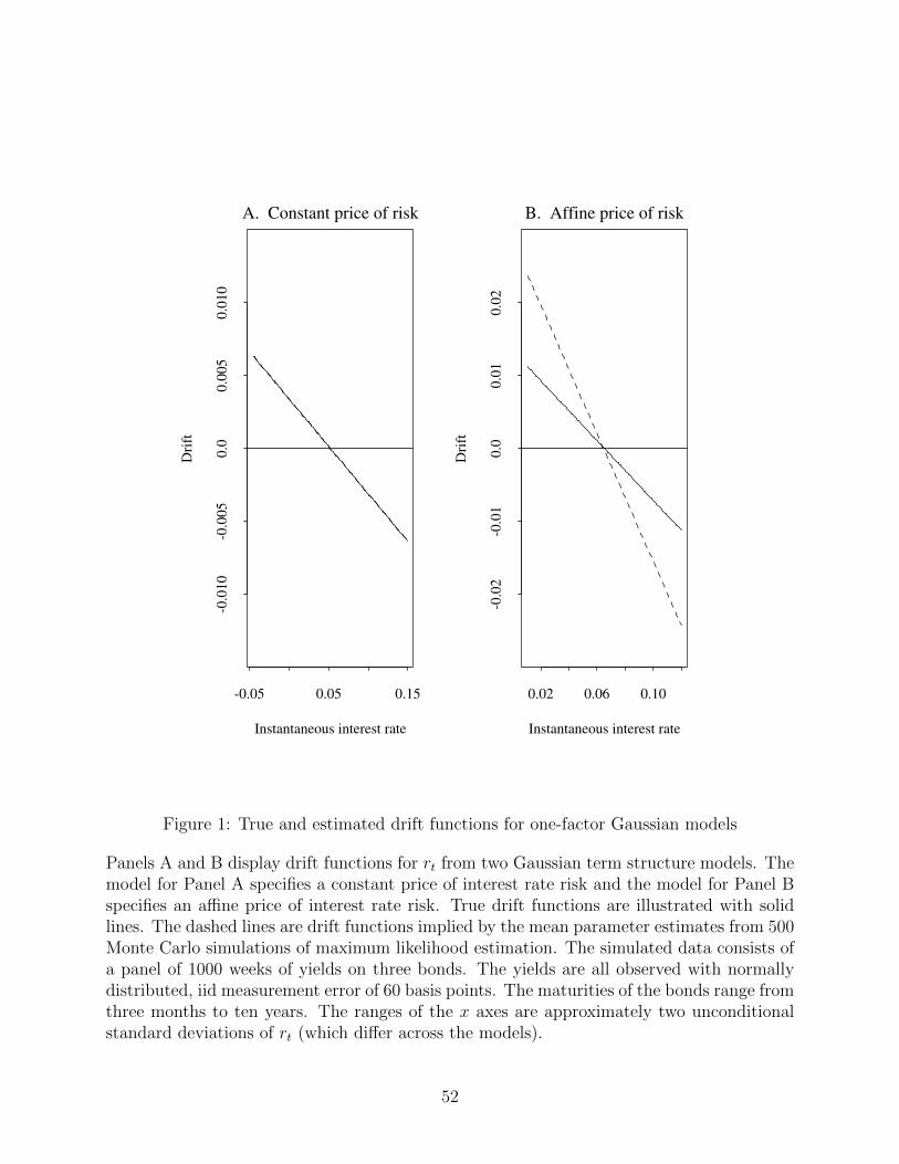
Instantaneous interest rate

Dri

ft

-0.05 0.05 0.15

-0.0

10-0

.005

0.0

0.00

50.

010

A. Constant price of risk

Instantaneous interest rate

Dri

ft

0.02 0.06 0.10

-0.0

2-0

.01

0.0

0.01

0.02

B. Affine price of risk

Figure 1: True and estimated drift functions for one-factor Gaussian models

Panels A and B display drift functions for rt from two Gaussian term structure models. Themodel for Panel A specifies a constant price of interest rate risk and the model for Panel Bspecifies an affine price of interest rate risk. True drift functions are illustrated with solidlines. The dashed lines are drift functions implied by the mean parameter estimates from 500Monte Carlo simulations of maximum likelihood estimation. The simulated data consists ofa panel of 1000 weeks of yields on three bonds. The yields are all observed with normallydistributed, iid measurement error of 60 basis points. The maturities of the bonds range fromthree months to ten years. The ranges of the x axes are approximately two unconditionalstandard deviations of rt (which differ across the models).

52

Instantaneous interest rate

Dri

ft

0.0 0.04 0.10

-0.0

10-0

.005

0.0

0.00

50.

010

A. Estimated model is linear

Instantaneous interest rate

Dri

ft

0.0 0.04 0.10

-0.0

10-0

.005

0.0

0.00

50.

010

B. Estimated model is nonlinear

Figure 2: True and estimated drift functions for a one-factor square-root model

Simulated data of 1000 weeks of yields on three bonds are generated by a one-factor translatedCIR model. The maturities of the bonds range from three months to ten years. One bond’syield is observed without error and the other bonds’ yields are observed with normallydistributed, iid measurement error of 60 basis points. The true model’s drift function for rtis indicated by the identical solid lines. The dashed lines are drift functions implied by meanparameter estimates from 500 Monte Carlo simulations of linearized instantaneous Kalmanfilter estimation. The estimated model in Panel A is a translated CIR model. The estimatedmodel in Panel B nests the translated CIR model by allowing for a nonlinear drift under thephysical measure.

53

Level

Dri

ft

0.0 0.04

-0.0

10-0

.005

0.0

0.00

50.

010

A. First state variable

Level

Dri

ft

0.0 0.04

-0.0

10-0

.005

0.0

0.00

50.

010

B. Second state variable

Figure 3: True and estimated drift functions for a two-factor nonlinear model

Simulated data of 1000 weeks of yields on three bonds are generated by a two-factor square-root diffusion model with nonlinear drifts. The maturities of the bonds range from threemonths to ten years. Two of the bonds’ yields are observed without error and the otherbond’s yield is observed with normally distributed, iid measurement error of 20 basis points.The true model’s drift functions for the state variables are indicated by the solid lines. Thedashed lines are drift functions implied by mean parameter estimates from 500 Monte Carlosimulations of simulated maximum likelihood.

54