estimation of defects based on defect decay model ed3 m

Estimation of Defects Based onDefect Decay Model: ED3M

Syed Waseem Haider, Student Member, IEEE, Joao W. Cangussu, Member, IEEE,

Kendra M.L. Cooper, Member, IEEE, and Ram Dantu, Member, IEEE

Abstract—An accurate prediction of the number of defects in a software product during system testing contributes not only to the

management of the system testing process but also to the estimation of the product’s required maintenance. Here, a new approach,

called Estimation of Defects based on Defect Decay Model (ED3M) is presented that computes an estimate of the total number of

defects in an ongoing testing process. ED3M is based on estimation theory. Unlike many existing approaches, the technique

presented here does not depend on historical data from previous projects or any assumptions about the requirements and/or testers’

productivity. It is a completely automated approach that relies only on the data collected during an ongoing testing process. This is a

key advantage of the ED3M approach as it makes it widely applicable in different testing environments. Here, the ED3M approach

has been evaluated using five data sets from large industrial projects and two data sets from the literature. In addition, a performance

analysis has been conducted using simulated data sets to explore its behavior using different models for the input data. The results are

very promising; they indicate the ED3M approach provides accurate estimates with as fast or better convergence time in comparison

to well-known alternative techniques, while only using defect data as the input.

Index Terms—Defect prediction, system testing, estimation theory, maximum likelihood estimator.

Ç

1 INTRODUCTION

SOFTWARE metrics are crucial for characterizing thedevelopment status of a software product. Well-defined

metrics can help to address many issues, such as cost,resource planning (people, equipment such as testbeds,etc.), and product release schedules. Metrics have beenproposed for many phases of the software developmentlifecycle, including requirements, design, and testing.

In this paper, the focus is on characterizing the status ofthe software testing effort using a single key metric: theestimated number of defects in a software product. Theavailability of this estimate allows a test manager toimprove his planning, monitoring, and controlling activ-ities; this provides a more efficient testing process. Also,since, in many companies, system testing is one of the lastphases (if not the last), the time to release can be betterassessed; the estimated remaining defects can be used topredict the required level of customer support.

Ideally, a defect estimation technique has several im-portant characteristics. First, the technique should beaccurate as decisions based on inaccurate estimates can betime consuming and costly to correct. However, mostestimators can achieve high accuracy as more and moredata becomes available and the process nears completion.

By that time, the estimates are of little, if any, use. Therefore,a second important characteristic is that accurate estimatesneed to be available as early as possible during the systemtesting phase. The faster the estimate converges to the actualvalue (i.e., the lower its latency), the more valuable theresult is to a test manager. Third, the technique should begenerally applicable in different software testing processesand on different kinds of software products. The inputs tothe process should be commonly available and should notrequire extensive expertise in an underlying formalism. Inthis case, the same technique can be widely reused, bothwithin and among software development companies,reducing training costs, the need for additional toolsupport, etc.

Many researchers have addressed this important pro-blem with varying end goals and have proposed estimationtechniques to compute the total number of defects. A groupof researchers focuses on finding error-prone modulesbased on the size of the module [1], [2], [3]. Briand et al.[4] predict the number of remaining defects duringinspection using actual inspection data, whereas Ostrandet al. [5] predict which files will contain the most faults inthe next release. Zhang and Mockus [6] use data collectedfrom previous projects to estimate the number of defects ina new project. However, these data sets are not alwaysavailable or, even if they are, may lead to inaccurateestimates. For example, Zhang and Mockus use a naivemethod based only on the size of the product to selectsimilar projects while ignoring many other critical factorssuch as project type, complexity, etc. Another alternativethat appears to produce very accurate estimates is based onthe use of Bayesian Belief Networks (BBNs) [7], [8], [9].However, these techniques require the use of additionalinformation, such as expert knowledge and empirical data,

336 IEEE TRANSACTIONS ON SOFTWARE ENGINEERING, VOL. 34, NO. 3, MAY/JUNE 2008

. S.W. Haider, J.W. Cangussu, and K.M.L. Cooper are with the Departmentof Computer Science, University of Texas at Dallas, Richardson, TX75083. E-mail: {easeem, cangussu, kcooper}@utdallas.edu.

. R. Dantu is with the Department of Computer Science and Engineering,University of North Texas, PO Box 311366, Denton, TX 76203.E-mail: [email protected].

Manuscript received 5 Feb. 2007; revised 3 Sept. 2007; accepted 21 Jan. 2008;published online 14 Apr. 2008.Recommended for acceptance by B. Littlewood.For information on obtaining reprints of this article, please send e-mail to:[email protected], and reference IEEECS Log Number TSE-0031-0207.Digital Object Identifier no. 10.1109/TSE.2208.23.

0098-5589/08/$25.00 � 2008 IEEE Published by the IEEE Computer Society

that are not necessarily collected by most software devel-opment companies. Software reliability growth models(SRGMs) [10], [11] are also used to estimate the totalnumber of defects to measure software reliability. Althoughthey can be used to indicate the status of the testing process,some have slow convergence while others have limitedapplication as they may require more input data or initialvalues that are selected by experts.

Defect prediction techniques proposed in the literaturecan quickly estimate highly accurate predictions; however,many have some limitations on their application in a widevariety of testing environments. To improve on the existingapproaches, in particular with respect to the applicability,the following characteristics are needed in a technique.First, it should use the defect count, an almost ubiquitousinput, as the only data required to compute the estimates(historical data are not required). Most companies, if not all,developing software have a way to report defects whichthen can be easily counted. Second, the user should not berequired to provide any initial values for internal para-meters or expert knowledge; this results in a fullyautomated approach. Third, the technique should beflexible; it should be able to produce estimates based ondefect data reported in execution time or calendar time.

A new estimator, referred to hereafter as Estimation ofDefects based on Defect Decay Model (ED3M), is a novelapproach proposed here which has been rigorouslyvalidated using case studies, simulated data sets, and datasets from the literature. Based on this validation work, theED3M approach has been shown to produce accurate finalestimates with a convergence rate that meets or improvesupon closely related, well-known techniques. The onlyinput is the defect data; the ED3M approach is fullyautomated.

Although the ED3M approach has yielded promisingresults, there are defect prediction issues that are notaddressed by it. For example, system test managers wouldbenefit from obtaining a prediction of the defects to befound in ST well before the testing begins, ideally in therequirements or design phase. This could be used toimprove the plan for developing the test cases. TheED3M approach, which requires test defect data as theinput, cannot be used for this. Alternate approaches whichrely on different input data (e.g., historical project data andexpert knowledge) could be selected to accomplish this.However, in general, these data are not available at mostcompanies. A second issue is that test managers may preferto obtain the predictions for the number of defects on afeature-by-feature basis, rather than for the whole system.Although the ED3M approach could be used for this, thenumber of sample points for each feature may be too smallto allow for accurate predictions. As before, additionalinformation could be used to achieve such estimations, butthis is beyond the scope of this paper. Third, theperformance of the ED3M approach is affected when thedata diverge from the underlying assumption of anexponential decay behavior. However, the results indicatethe estimations are still useful under these conditions; theseresults are presented in Section 5.

The remainder of this paper is organized as follows: Anoverview of estimation theory is provided as background inSection 2. A description of the ED3M approach is presentedin Section 3. The validation of the approach using casestudies is presented in Section 4, and a performanceanalysis using simulated test data is presented in Section 5.Section 6 presents a survey of the related work along withquantitative comparisons with three relevant techniquesusing data sets from the literature. Section 7 contains theconclusions and future work.

2 ESTIMATION THEORY OVERVIEW

Numerous application areas, such as signal processing,defect estimation, and software reliability, need to extractinformation from observations that have been corrupted bynoise. For example, in a software testing process, theobservations are the number of defects detected; the noisemay have been caused by the experience of the testers, sizeand complexity of the application, errors in collecting thedata, etc. The information of interest to extract from theobservations is the total number of defects in the software.A branch of statistics and signal processing, estimationtheory, provides techniques to accomplish this.

The concepts of the data, noise, and information toextract are represented mathematically below. In this work,square brackets are used to denote a random quantity (e.g.,x½n� and w½n� in (1)) and parentheses to denote adeterministic quantity (e.g., RðtÞ and efðtÞ in (79)).

Mathematically, the observations are an N-point data setrepresented as the vector x, or x½0�; x½1�; . . . ; x½N � 1�. Theinformation to extract from the data set is the scalarparameter �. The noise is represented as the vector w, orw½0�; w½1�; . . . ; w½N � 1�. For a simple linear model, as in (1),the parameter � is linearly related to the observation, i.e.,each observation is the sum of the parameter and noise.Linear models are used in a wide variety of estimationproblems for two main reasons: They provide a closed formsolution for the problem and the statistical performance isthoroughly studied:

x½n� ¼ �þ w½n�: ð1Þ

Using vector notation, the linear model is presented in(2). Once again, � is linearly related to the observations:

x ¼ 1�þw: ð2Þ

In the model given by (2), the noise is White Gaussian(Normal) random noise [12], w½n� � N ½0; �2�, of zero meanand variance �2 at an instant n. The noise componentsw½0�; w½1�; . . . ; w½N � 1� are observed at different instants oftime; they are assumed to be identically independentlydistributed (iid) Gaussian random variables. The iidassumption is an established, simplifying assumption,which means the Cross Correlation E½w½n� � w½n� 1�� ofthe noise components is 0. Hence, there is no interferenceamong the noise components. The iid assumption helps toobtain a closed form solution (refer to (21)).

A more general form of the linear model is presented in

x ¼ H�þw; ð3Þ

HAIDER ET AL.: ESTIMATION OF DEFECTS BASED ON DEFECT DECAY MODEL: ED3M 337

where xN�1 is the data vector, HN�P is the observation matrix,

�P�1 is the parameter vector to be estimated, and wN�1 is the

noise vector with a Normal distribution � N ½0; �2�.Given a data set of observations, x, the problem is to

estimate �. In other words, an estimator � is needed (refer to

(4)) that is a function of the data set x. There are a number of

ways to find this function. The approaches consider factors

including the type of data model, prior information known

about the function, etc. [13]:

� ¼ g x½0�; x½1�; . . . ; x½N � 1�ð Þ: ð4Þ

There are several steps needed to define an estimator.

The first step is to select the model relating the observations,

parameter �, and noise. As discussed above, a linear model

has a number of advantages and is typically selected.

Second, as the data are inherently random (refer to (2)), the

distribution of the data set needs to be modeled. A Normal,

or Gaussian, random variable with mean m and variance �2,

N ½m;�2�, is often assumed. The equation for the probability

density function (PDF) of the Normal distribution is used to

begin with [13]:

fðxÞ ¼ 1

ð2��2Þ12

e�1

2�2ðx�mÞ2

: ð5Þ

In the estimation problem, a PDF is a function of both

data and a value of �. The result of substituting for x and

mean m in (5) with x½n� and �, respectively, is shown in

p x½n�; �ð Þ ¼ 1

ð2��2Þ12

e �1

2�2 x½n��ð Þ2� �

: ð6Þ

Extending this to consider the vector ofN observations, x,

the result is (7). The joint probability distribution of data,

pðx; �Þ, is a function of both data x and unknown parameter �;

this is also called a likelihood function:

pðx; �Þ ¼ 1

ð2��2ÞN2

e �1

2�2

PN�1

n¼0x½n��ð Þ2

� �: ð7Þ

The third step is to define an accurate, realizable

estimator. The bias and variance are two characteristics

used to determine the accuracy of an estimator. The mean of

the square of the error (mse) of �, given by (8), is a natural

accuracy criteria to begin with. Algebraic manipulations in

(9) lead to (10), which shows that the mse of � is equivalent

to the sum of the variance and the square of the bias of �.

Consequently, in order to improve the accuracy of �, it is

necessary to minimize the variance of � and reduce the bias

to zero. When the bias is reduced to zero, the estimator is

called unbiased; the estimator determines the true value of

the unknown parameter � on average:

mseð�Þ ¼ E ð�� Þ2h i

; ð8Þ

mseð�Þ ¼ E �� Eð�Þ� �

þ Eð�� Þ� �h i2

� �

¼ V ARð�Þ þ Eð�Þ � �h i2

;

ð9Þ

mseð�Þ ¼ V ARð�Þ þ bias of �h i2

: ð10Þ

Once an unbiased estimator is chosen, only the variancearound the parameter � dictates the accuracy of theestimator. If the lower bound on the variance of anestimator can be found, then the challenge becomes to findan estimator � with a variance that is closest to the lowerbound. In the best-case scenario, an estimator with avariance equivalent to the lower bound is found. This iscalled an efficient estimator. The theorem that provides thelower bound on the variance of the estimator is the Cramer-Rao Lower Bound (CRLB) Theorem:

CRLB Theorem [13]. It is assumed that the PDF pðx; �Þsatisfies the regularity condition in

E@lnpðx; �Þ

@�

� ¼ 0; 8�; ð11Þ

where the expectation is taken with respect to pðx; �Þ. Then,the variance of any unbiased estimator � must satisfy

V ARð�Þ � 1

�E @2lnpðx;�Þ@�2

h i : ð12Þ

An estimator, �, that is unbiased and satisfies the lowerbound given by (12) is called an efficient minimum varianceunbiased (MVU) estimator. The efficient MVU estimatorand its minimum variance, defined by (14) and (15), can befound iff (13) holds:

@lnpðx; �Þ@�

¼ Ið�Þ gðxÞ � �ð Þ; ð13Þ

where � ¼ gðxÞ ð14Þ

and V AR ð�Þ ¼ 1

Ið�Þ : ð15Þ

It is important to note that an efficient MVU estimatordoes not always exist or, if one does exist, it is not alwayspossible to find it. An example of one that can be found ispresented here. An MVU estimator for � in (1) is foundusing the CRLB Theorem [13] (refer to (16), (17), and (18):

@lnpðx; �Þ@�

¼ N

�2

1

N

XN�1

n¼0

x½n� � � !

; ð16Þ

where � ¼ 1

N

XN�1

n¼0

x½n� ð17Þ

and VAR ð�Þ ¼ �2

N: ð18Þ

The distribution of � is � � N ½�; �2

N �. The estimator in (17)

is unbiased, E½�� ¼ �, and achieves the CRLB on its

variance, �E½@2lnpðx;�Þ@�2 � ¼ N

�2 . Hence, � is an efficient MVU

estimator.In the cases where an efficient MVU estimator does not

exist or cannot be found, an alternative approach is needed.The Maximum Likelihood Estimation (MLE) is based on the


maximum likelihood principle. It is a popular approach toobtain practical estimators [13]. An MLE obtains anestimator that is approximately the efficient MVU estima-tor. In other words, MLE is asymptotically unbiased,achieves CRLB on its variances, and has a Gaussian PDF.For a linear model, MLE achieves the CRLB with a finitedata set. This is discussed further in Section 3.

The MLE provides a value of the scalar parameter �

which maximizes the likelihood function, pðx; �Þ, for a fixed

x over the range of �. An important property of MLE is that,if an efficient estimator exists, then MLE will produce it. Forthe model in (3), a value of � exists which maximizes thelikelihood function, pðx; �Þ, if the second derivative of loglikelihood function with respect to � is negative:

@2lnpðx; �Þ@�2

< 0: ð19Þ

Using the maximization technique, the log likelihoodfunction is differentiated with respect to �; it is solved for �by equating it to 0 (refer to (20) and (21)). Note that (21) hasthe form of (3):

@lnpðx; �Þ@�

¼ 0; ð20Þ

� ¼ ðHTHÞ�1HTx: ð21Þ

3 PROPOSED APPROACH: ED3M

3.1 Overview

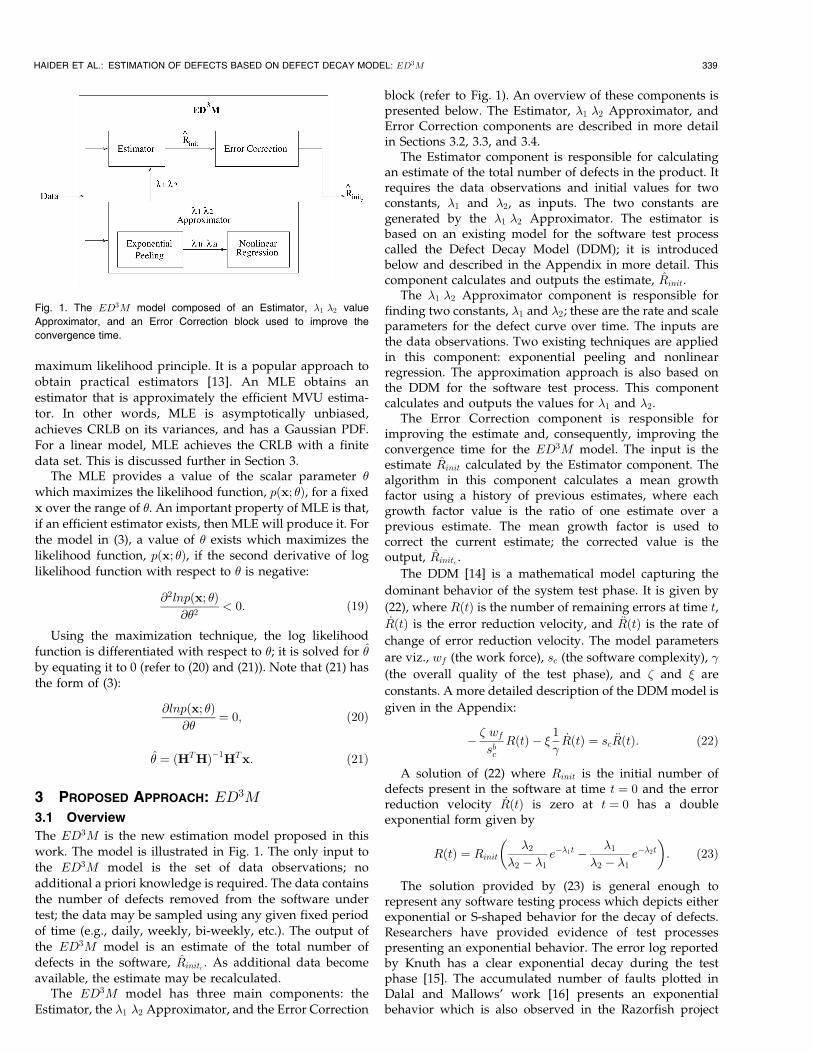
The ED3M is the new estimation model proposed in thiswork. The model is illustrated in Fig. 1. The only input tothe ED3M model is the set of data observations; no

additional a priori knowledge is required. The data containsthe number of defects removed from the software undertest; the data may be sampled using any given fixed periodof time (e.g., daily, weekly, bi-weekly, etc.). The output ofthe ED3M model is an estimate of the total number ofdefects in the software, Rinitc . As additional data becomeavailable, the estimate may be recalculated.

The ED3M model has three main components: theEstimator, the �1 �2 Approximator, and the Error Correction

block (refer to Fig. 1). An overview of these components ispresented below. The Estimator, �1 �2 Approximator, andError Correction components are described in more detailin Sections 3.2, 3.3, and 3.4.

The Estimator component is responsible for calculatingan estimate of the total number of defects in the product. Itrequires the data observations and initial values for twoconstants, �1 and �2, as inputs. The two constants aregenerated by the �1 �2 Approximator. The estimator isbased on an existing model for the software test processcalled the Defect Decay Model (DDM); it is introducedbelow and described in the Appendix in more detail. Thiscomponent calculates and outputs the estimate, Rinit.

The �1 �2 Approximator component is responsible forfinding two constants, �1 and �2; these are the rate and scaleparameters for the defect curve over time. The inputs arethe data observations. Two existing techniques are appliedin this component: exponential peeling and nonlinearregression. The approximation approach is also based onthe DDM for the software test process. This componentcalculates and outputs the values for �1 and �2.

The Error Correction component is responsible forimproving the estimate and, consequently, improving theconvergence time for the ED3M model. The input is theestimate Rinit calculated by the Estimator component. Thealgorithm in this component calculates a mean growthfactor using a history of previous estimates, where eachgrowth factor value is the ratio of one estimate over aprevious estimate. The mean growth factor is used tocorrect the current estimate; the corrected value is theoutput, Rinitc .

The DDM [14] is a mathematical model capturing the

dominant behavior of the system test phase. It is given by

(22), where RðtÞ is the number of remaining errors at time t,_RðtÞ is the error reduction velocity, and €RðtÞ is the rate of

change of error reduction velocity. The model parameters

are viz., wf (the work force), sc (the software complexity), �

(the overall quality of the test phase), and � and � are

constants. A more detailed description of the DDM model is

given in the Appendix:

� � wfsbc

RðtÞ � � 1

�_RðtÞ ¼ sc €RðtÞ: ð22Þ

A solution of (22) where Rinit is the initial number ofdefects present in the software at time t ¼ 0 and the errorreduction velocity _RðtÞ is zero at t ¼ 0 has a doubleexponential form given by

RðtÞ ¼ Rinit�2

�2 � �1e��1t � �1

�2 � �1e��2t

�: ð23Þ

The solution provided by (23) is general enough torepresent any software testing process which depicts eitherexponential or S-shaped behavior for the decay of defects.Researchers have provided evidence of test processespresenting an exponential behavior. The error log reportedby Knuth has a clear exponential decay during the testphase [15]. The accumulated number of faults plotted inDalal and Mallows’ work [16] presents an exponentialbehavior which is also observed in the Razorfish project


Fig. 1. The ED3M model composed of an Estimator, �1 �2 value

Approximator, and an Error Correction block used to improve the

convergence time.

[14]. Jacoby and Tohma’s reliability growth model [17]presents cases of both exponential and S shaped curves.Additionally, Ehrlich et al. [18] present examples ofexponentially accumulated failure and failure intensitydecay. The data sets in [14], [19], [20] also exhibitexponential behavior.

3.2 Computing the Estimator

As stated earlier, the overall behavior of the decay of defectsin the ST phase is assumed to have a double exponentialformat as in (23). Equation (23) has been rewritten, whereRðnÞ is the number of remaining defects at the nth time unit:

RðnÞ ¼ Rinit�2

�2 � �1e��1n � �1

�2 � �1e��2n

�: ð24Þ

RðnÞ is the number of remaining defects at day (or anyother fixed time interval) n after removing defects atday n� 1. Rinit is the total or initial number of defectspresent in the software product. The values of �1 and �2 arecalculated by the �1 �2 Approximator; this component isdiscussed in Section 3.3.

Assume now that the defects removed at any day k aregiven by dðkÞ. The relationship between RðnÞ and dðkÞ isgiven by

RðnÞ ¼ Rðn� 1Þ � dðn� 1Þ; ð25Þ

RðnÞ ¼ Rinit �Xn�1

k¼0

dðkÞ; ð26Þ

or simply as given by

RðnÞ ¼ Rinit �DðnÞ; ð27Þ

where DðnÞ ¼Xn�1

k¼0

dðkÞ ð28Þ

for 0 � dðnÞ � Rinit �DðnÞ. Now, solving (24) and (27) forDðnÞ, which represents the total number of defects removedfrom the product under test in n days, leads to

DðnÞ ¼ Rinit 1� �2

�2 � �1e��1n þ �1

�2 � �1e��2n

�: ð29Þ

The model defined by (24) to (29) is deterministic, i.e., itdoes not account for random variations. However, noiseand unforeseen perturbations are common place in thesoftware testing process and a deterministic model cannotcapture this stochastic behavior. There are multiple sourcesfor these variations, such as work force relocation, noise inthe data collection process, test of “complex or poorlyimplemented” parts of the system, multiple reports of thesame error, among others. A random variable that consistsof the sum of a large number of small random variables(various sources of noise) under general conditions can beapproximated by Gaussian random variable [12]. Because ofthis, the Gaussian distribution finds its use in a wide varietyof man-made and natural phenomena. Therefore, randombehavior is incorporated into the model by adding arandom error defined by White Gaussian noise [12],z½k� � N ½0; 2�, in defects removed every day, as given by

�d½k� ¼ dðkÞ þ z½k�: ð30Þ

Note that the form of (30) is similar to (1) and itrepresents the data set obtained from the field. D½n� from(28) is now redefined as a Gaussian random variable (referto (31)) using �d½k� from (30):

D½n� ¼Xn�1

k¼0

�d½k� ¼Xn�1

k¼0

dðkÞ þXn�1

k¼0

z½k�: ð31Þ

Using (28), (29), and (31), D½n� is given by

D½n� ¼ Rinit 1� �2

�2 � �1e��1n þ �1

�2 � �1e��2n

�þXn�1

k¼0

z½k�;

ð32Þ

where z½0�; . . . ; z½n� 1� are iid zero mean Gaussian randomvariables. These have been incorporated to model randomnoise that affects the system test process.

As discussed earlier, a wide variety of external andinternal factors can affect the software testing process. Aneffort to individually account for each such factor will resultin a large number of random variables and, in turn, a verycomplex mathematical model. The resulting model wouldbecome even more complex when the interference of theserandom variables with each other is considered. Theinterference may occur within one data set or amongdifferent data sets collected over time.

Hence, the model is simplified by first assuming that aGaussian noise affects the whole testing process identically.Moreover, the samples taken at different instants areindependent of each other. Note that the assumptions madehere are collectively called iid. These simplifying assump-tions have been established and utilized by the community,as in [21], [22], [23].

The application of the central limit onPn�1

k¼0 z½k� in (31)leads to

w½n� ¼Xn�1

k¼0

z½k�; ð33Þ

where w½n� � N ½0; �2�. Substituting w½n� in (32) results in

D½n� ¼ Rinit 1� �2

�2 � �1e��1n þ �1

�2 � �1e��2n

�þ w½n�:

ð34Þ

The derivation of an estimator for (34) would incur thecomputation of three parameters Rinit, �1, and �2 together,which is a complex computation. The problem is simplifiedby first computing an approximation for �1 and �2 (refer toSection 3.3 for details). The approximated values are thenused to compute hðnÞ in

hðnÞ ¼ 1� �2

�2 � �1e��1n þ �1

�2 � �1e��2n: ð35Þ

The simplified problem is now defined in

D½n� ¼ RinithðnÞ þ w½n�: ð36Þ

Writing (36) in vector form in (37), where D, h, and w arevectors of dimensions N � 1:

D ¼ Rinithþw: ð37Þ


The PDF of D½n� using (5) is given by

p D½n�;Rinitð Þ ¼ 1

ð2��2Þ12

e �1

2�2 D½n��RinithðnÞð Þ2� �

: ð38Þ

Following (7), the PDF of D is

pðD;RinitÞ ¼1

ð2��2ÞN2

e �1

2�2

PN�1

n¼0D½n��RinithðnÞð Þ2

� �

¼ 1

ð2��2ÞN2

e �1

2�2ðD�RinithÞT ðD�RinithÞ� �

:

ð39Þ

To find the estimator, Rinit, of Rinit, the ln of (39) is taken,

which simplifies the equation. Then, the resulting (40) is

maximized with respect to Rinit:

ln pðD;RinitÞ ¼ �N

2lnð2��2Þ � 1

2�2

XN�1

n¼0

D½n� �RinithðnÞð Þ2:

ð40Þ

Using the maximization technique as given in (20), the

partial derivative of (40) with respect to Rinit is taken in

@lnpðD;RinitÞ@Rinit

¼ 1

�2

XN�1

n¼0

D½n� �RinithðnÞð ÞhðnÞ: ð41Þ

Then, the partial derivative is equated to 0 in (42) and

solved for the estimator Rinit. The lemma given below

proves that R0 is indeed a maximization function:

XN�1

n¼0

D½n� � RinithðnÞ�

hðnÞ ¼ 0; ð42Þ

Rinit ¼PN�1

n¼0 D½n�hðnÞð ÞPN�1n¼0 h

2ðnÞ: ð43Þ

Alternately, (43) can be written in vector form as given by

Rinit ¼ ðhThÞ�1hTD: ð44Þ

Lemma. @2ln pðD;RinitÞ@R2

init

¼ � 1�2 h

2ðnÞ; hence, Rinit is indeed a

maximization value, as presented in (19).

3.3 �1 �2 Approximator

As stated before, computing the estimator using threeunknowns, Rinit, �1, and �2, leads to a very complexsolution. To avoid this situation, the �1 �2 Approximatorapproximates the values of �1 and �2, which are then usedin (43); this approach simplifies the problem to determineone unknown, Rinit.

The �1 �2 Approximator uses two steps. The first step isto find the initial values �1i and �2i using a technique calledExponential Peeling [24]. These initial values are thenprovided as input to a nonlinear regression method in thesecond step. The nonlinear regression, which is implemen-ted using the Gauss-Newton method with the Levenberg-Marquardt modification [24], results in the values of �1 and�2 that are used in the “Estimator” block.

Exponential Peeling. The Exponential Peeling techniqueis used to find the initial values �1i and �2i . The defect datais modeled by (30). Assuming that the total number ofdefects, Rp

init, up to time k ¼ n� 1 is given by the data set,�d½0�; �d½1�; . . . ; �d½n� 1�, as in

Rpinit ¼ D½n� ¼

Xn�1

k¼0

�d½k�: ð45Þ

Without loss of generality, (24) is normalized by Rpinit

(refer to (46)), where CðkÞ is a normalized version of RðkÞand k : 0 � k � ðn� 1Þ:

CðkÞ ¼ RðkÞRpinit

¼ �2

�2 � �1e��1k � �1

�2 � �1e��2k

�: ð46Þ

Equation (46) is a nonlinear double exponential equation.

Note that (46) will provide the same result whether �1 < �2 or

vice versa. Only for explanation purposes is�1 < �2 assumed.

Therefore, as time increases, the component �1

�2��1e��2n of (46)

diminishes faster, leaving only �2

�2��1e��1n component. Hence,

for k : ðn�1Þ2 < k � ðn� 1Þ, CðkÞ is given by

CðkÞ ’ �2

�2 � �1e��1k: ð47Þ

Equation (47) is linearized by taking log, as shown inFig. 2. The data points in Figs. 2 and 3 belong to the same


Fig. 2. Finding �1i for k : ðn�1Þ2 < k � ðn� 1Þ. Fig. 3. Finding �2i for k : 0 � k � ðn�1Þ

2 .

data set presented in Fig. 5 (case study 1). The resulting

curve can be approximated by a straight line, as given by

(48); the slope of this line is m1 ¼ ��1i :

logðCðkÞÞ ’ ��1kþ log�2

�2 � �1

�’ m1kþ b1: ð48Þ

Or, in exponential form,

�2

�2 � �1e��1k ’ em1k � eb1 : ð49Þ

Hence, the initial value �1i can be determined.

Next, �2 is determined. For k : 0 � k � ðn�1Þ2 , CðkÞ is given

by (46). If (46) is subtracted from the right-hand side of (49),

then the result is approximately �1

�2��1e��2n, as given in

em1k � eb1 � �2

�2 � �1e��1k � �1

�2 � �1e��2k

�’ �1

�2 � �1e��2n:

ð50Þ

Equation (50) is linearized by taking log, as shown in

Fig. 3; the resulting curve can be approximated by a straight

line as given by (51). The slope of this line is m2 ¼ ��2i :

log�1

�2 � �1e��2k

�¼ ��2kþ log

�1

�2 � �1

�’ m2kþ b2:

ð51Þ

Therefore, the initial approximation for �2i can be found

as well.The values �1i and �2i computed using the exponential

peeling are not accurate enough to be directly used by the

estimator. However, they have been shown to be reasonably

good to be used as initial values for nonlinear regression

methods [24].

Nonlinear regression. The second step is to use a

nonlinear regression technique to compute the final

approximations of �1 and �2, as shown in Fig. 1. Let

��T ¼ ½�1 �2�, then rewriting (46) as a function of �� leads to

Cðk; ��Þ ¼ �2

�2 � �1e��1k � �1

�2 � �1e��2k

�: ð52Þ

The Taylor series expansion of Cðk; ��Þ with initial values

��ðiÞT ¼ ½�1i �2i � is given in (53). Note that Cðk; ��Þ is written

in vector form w.r.t. k:

Cð��Þ ’ C ��ðiÞ� �

þ@C ��ðiÞ� �@��T

�� ðiÞ� �

: ð53Þ

The data set R½k�; 0 � k � ðn� 1Þ can be written in the

vector form R w.r.t. k as well. The least square error

k RRpinit�Cð��Þk2 ¼ 0, is minimized w.r.t. ð�� ðiÞÞ, which

results in the residual error "ðiÞ and the Gauss-Newton

algorithm given in

"ðiÞ ¼ FðiÞTFðiÞ� ��1

FðiÞT � R

Rpinit

�C ��ðiÞ� � �

; ð54Þ

��ðiþ1Þ ¼ ��ðiÞ þ "ðiÞ; ð55Þ

where FðiÞ is given by

FðiÞ ¼@C ��ðiÞ� �@��T

: ð56Þ

As "ðiÞ and ��ðiþ1Þ have been found using ��ðiÞ, "ðiþ1Þ and��ðiþ2Þ can be found using ��ðiþ1Þ. These steps are repeateduntil " � 10�8. Each iteration returns the new values of ��T ¼½�1 �2� after adding ".

Sometimes FðiÞTFðiÞ matrices are singular or ill condi-tioned. To overcome this obstacle, the Levenberg-Mar-quardt algorithms have been used. A more detailedexplanation on the Gauss-Newton method with the Leven-berg-Marquardt modification is given in [24].

3.4 Error Correction

The accuracy of an estimator is heavily dependent on the dataset provided. For example, with few initial points in a data set,it is very difficult to produce highly accurate estimates. Errorcorrection techniques are used to improve the estimates and,consequently, reduce the convergence time.

The error correction technique in the ED3M modeliteratively determines a mean growth factor, which is usedto compensate for the error. The technique is described below.

Assume two predictions, Rinitðt ¼ iÞ and Rinitðt ¼ jÞ, areavailable, where j� i ¼ �t and �t > 0. A growth factor ejfor estimation Rinitðt ¼ jÞ can be computed with

ej ¼Rinitðt ¼ jÞRinitðt ¼ iÞ

: ð57Þ

The growth factor ej is greater than one, as (43) is anincreasing function. In the testing process, data are collectedover time. As more defects are discovered, the resultingestimate determined by (43) also increases.

The growth factor ej may result in a very high or verylow correction value. To minimize the sharp effect, themean of previously found growth factors ranging from ej toej�ð�tþ1Þ is calculated using

mj ¼ej þ . . .þ ej�ð�tþ1Þ

�tþ 1: ð58Þ

The mean growth factor, mj, can now be used to scale(compensate) the estimate R0ðt ¼ jÞ to find the correctedestimate Rinitcðt ¼ jÞ, as in

Rinitcðt ¼ jÞ ¼ mj � R0ðt ¼ jÞ: ð59Þ

Note that, when j� 1 < �t, then ej ¼ Rinitðt¼jÞRinitðt¼1Þ and mj ¼ ej.

It should be noted that the time difference �t betweentwo estimations influences the results of the correctionalgorithm. A small time difference may result in a sequenceof small changes in the estimation. While this would bedesired for the control/analysis of a physical system, asoftware process cannot be changed on a daily basis andmore time is needed to evaluate and perform correctiveactions (schedule or work force changes, for example) inview of the predictions. On the other hand, a large timedifference may result in a potential problem of beingdiscovered too late. An optimal time difference appears tobe project dependent, but its analysis is beyond the scope of


this paper. For the projects discussed in Section 4 and the

simulations in Section 5, the time difference �t ¼ 2 has been

used. �t ¼ 2 is greater than the smallest possible value,

which is 1, and is smaller than 3, which causes latency. The

value �t ¼ 2 has performed well for all industrial data sets

and simulation data sets. Experiments with other values,

such as 3 and 4, have been conducted, but they caused

latency.

3.5 Practical Application of the ED3M Approach

In practice, a test manager can use the defect data to plot the

(corrected) estimation curve; this plot can be used to

determine how long it would take to achieve prespecified

goals. For example, consider a project (as presented in

Section 4, case study 1), in which 35 days of testing have

passed; in this case, the estimation of Rinitc ¼ 804 defects. As

illustrated in Fig. 4, the curve of the defect decay using the

estimated number of defects can be plotted; this is the solid

line in the figure.Using the value of Rinitc , a plot of RðnÞ can be made

which estimates the future decay of defects over time; this is

the dashed line in the figure. It can be used to estimate the

number of days needed to reduce the number of defects to a

desired level. More specifically, RðnÞ is calculated using

(60), which is (24) with Rinit replaced by Rinitc . Substituting

the values of Rinitc , �1, and �2 into (60), n is incremented to

plot RðnÞ. For example, the plot in Fig. 4 shows that it

would take about n ¼ 130 days to reduce the number of

defects by 98 percent of the initial value. The manager can

use this information to adjust the testing process (try to

speed up the process) or the goals (increase the acceptable

number of remaining defects). Although not the focus of the

current research, a user-friendly decision support tool could

be developed for test managers with the capability to

generate these plots:

RðnÞ ¼ Rinitc

�2

�2 � �1e��1n � �1

�2 � �1e��2n

�: ð60Þ

4 CASE STUDIES

The ED3M approach has been applied to five case studies.These studies are large industrial projects from three differentcompanies. The projects include, among others, networkmanagement systems and programming language transla-tors. The size of the products ranges from 100 thousand linesof code (KLOC) to 500 KLOC. The numbers of defects ineach case study are: Case study 1 has 713 defects and117 number of data points, case study 2 has 476 defects and93 number of data points, case study 3 has 104 defects and97 number of data points, case study 4 has 553 defects and144 number of data points, and case study 5 has 257 defectsand 101 number of data points.

The estimates from the application of the ED3Mapproach are compared to the number of defects accumu-lated up to the product’s release time. Although this is notan exact measure of the total number of defects, it is a veryclose approximation for the case studies presented here.The number of defects discovered in the field after releasingthe product is reported as approximately 10 percent morefor the case studies presented in this section. This value isdependent on the operational profile used. That is, thelarger the difference between the user operational profileand the ST profile, the larger the impact on the accuracy ofED3M. As discussed later in Section 7, the “noise” on anoperational profile definition could be used to account forthis difference. Changes in the operational profile duringsystem testing are already absorbed by the collected datawhen computing the estimates.

The ED3M approach, described in Section 3, is incre-mentally applied to each data set using fixed increments offive units of time (or five elements from the data set). Here,this represents the test data from five working days. Aninitial assumption is that only the first five data points areavailable to compute the approximation for �1, �2, Rinit, andRinitc . Subsequently, five more elements from the data setare added and �1, �2, Rinit, and Rinitc are recomputed. Thisprocess is repeated until the data set is exhausted. Thisincremental approach allows for the evaluation of theconvergence of ED3M. That is, the less data required toachieve an accurate prediction, the better. Note that the totalnumber of elements in the data set gives the length ofsystem testing in units of time.

The results of the case studies are presented in Figs. 5, 6,7, 8, and 9; a summary is presented in Table 1. In each of thefigures, the estimation curve called Rinit is shown with athick broken line against the units of time. The errorcorrection is applied to the Rinit and the resulting curve,Rinitc , is shown with a thick solid line. Recall that thecorrected estimation curve is the output of the ED3Mapproach. Also, a constant line representing the actual totalnumber of defects found during system testing is drawn oneach figure to provide a visual reference. In addition, eachof the graphs has reference lines included for four absoluteerror measures: þ20 percent, �20 percent, þ30 percent, and�30 percent. These are referred to as tolerances in thediscussion. These relatively large tolerances have beenselected for use in the discussion recognizing that 1) a goodestimator will converge and produce very accurate esti-mates given time and 2) the earlier useful defect predictions


Fig. 4. Defect decay data and estimated curve for case study 1 using

only 35 data points.

can be made, the more valuable the approach is. Given thatestimators become more accurate as the testing processproceeds, the estimates calculated earlier are expected tohave a larger error. After the estimator reaches thesetolerance levels (e.g., 30 percent, then 20 percent, etc.), theresults are expected to continue to improve, or stabilize,with a lower error.

The results of the case studies are interesting as they

reveal the variability in the ED3M approach’s convergence

time and accuracy. To understand the performance of the

ED3M approach with respect to the alternative techniques

available, a comparative study is necessary; one has been

conducted and is presented in Section 6.2.


Fig. 7. Results for the incremental estimation of defects for case study 3.



TABLE 1Data Statistics for Five Different Case Studies

from Three Different Companies


The results of the case studies can be grouped as the best,good, and the worst. The results of case study 1 and casestudy 2 (Figs. 5 and 6) are the best, both for the timerequired to reach an accuracy tolerance and the finalestimate for the number of defects. In Fig. 5, the Rinitc

reaches the range of Rinit with 20 percent tolerance(absolute error) using less than 20 percent of the testingtime. The accuracy increases as more data become availablefor the estimation; Fig. 5 shows that ED3M is converging. Itcan be seen in Fig. 5 that the ED3M estimate converges to2.2 percent tolerance. This final point is referred to as theSystem Testing (ST) accuracy achieved. In case study 2, theRinitc reaches Rinit with 20 percent tolerance using25 percent of the testing time. Again, the accuracy increasesas more data becomes available; Fig. 6 also shows thatED3M is converging. The ST accuracy achieved by ED3Mis 5.8 percent tolerance. This means that the estimatednumber of defects is 105.8 percent of Actual ST Defects,which is a reasonable accuracy as there are, in this case, arelatively small number defects that testing is unable todiscover.

The results of case study 3 and case study 5 (Figs. 7 and9) are very similar and can be characterized as good, bothfor the time required to reach an accurate tolerance and thefinal estimate for the number of defects. In Fig. 7, the Rinitc

reaches Rinit with 20 percent tolerance using 36 percent ofthe testing time; case study 5 (Fig. 9) is 34 percent. In both ofthese studies, the accuracy increases as more data becomeavailable; the ST converges to 6 percent.

The results of case study 4 (Fig. 8) are the worst amongthe five, both for the time required to reach an accuracytolerance and the final estimate for the number of defects.The Rinitc reaches Rinit with 20 percent tolerance using41.3 percent of the testing time. The accuracy increases asmore data become available for the estimation; the STconverges to 7.2 percent. The results of this case study arediscussed in more detail in Section 4.1.

A consistent behavior of Rinit is observed in all casestudies, as shown in Figs. 5, 6, 7, 8, and 9. Rinit is alwaysincreasing and it starts slowly converging to a certain value.This tends to happen toward the end of the system testingphase. Such behavior of Rinit complies with generalbehavior of system testing. Hence, Rinit is a growingfunction of the defect data or the data set, whereas theerror correction technique discussed in Section 3.4 is proneto oscillations or variations in Rinitc , as shown in Fig. 6. This

is due to the effect of uneven growth of ej on Rinitc in the

presence of noise. The effect of a single growth factor ej on

Rinitc has been minimized by using mean growth factor mj.Overall, the results in columns 2 and 3 of Table 1 show

that ED3M converges to the specified tolerances using less

than 50 percent of the testing time for all of the case studies.

ED3M converged to 20 percent tolerance for three case

studies using 35 percent or less of the total project time.1 For

two case studies, ED3M used between 36 percent and

42 percent of the testing time to achieve the desired

accuracy for the estimates. As expected, if the tolerance is

relaxed from 20 percent to 30 percent, then the

convergence time decreases (i.e., improves), as can be seen

in Table 1. Except for case study 4, ED3M converged using

less than 35 percent of the total project time to reach the

30 percent.The last column in Table 1 provides the ST or final accuracy

(computed at the last data point in the data set) achieved for

each data set. The purpose of discussing the ST accuracy for

each data set is to show that ED3M indeed converges to the

Rinit present in the software. The lower accuracy of case

study 4, which is 7.2 percent, is due to its specific data

characteristics; these are discussed in Section 4.1. For case

study 1, the estimated defects are 2.2 percent more than the

Rinit; similarly, for case studies 2, 3, and 5, nearly 6 percent

more defects are found than the Rinit.An important observation in Table 1 is that, for all case

studies, ED3M estimated more defects than the actual

number of defects, which agrees with the general under-

standing of software testing that testing cannot find all of

the defects present in the software; consequently, there are

hidden defects in the software even after testing. Therefore,

ED3M is hinting toward these hidden defects. In addition,

the use of the Error Correction technique to calculate Rinitc

consistently improves the estimation results.

4.1 Discussion on Potential Limitations

As seen in the results for the case studies, the convergence

rate and accuracy of the ED3M approach have some

variability. Fig. 10 (case study 1) and Fig. 11 (case study 4)

are presented here to illustrate some potential limitations

when using the ED3M approach. Figs. 10 and 11 are


Fig. 10. (a) Distribution of defects over time. (b) Distribution of the remaining number of defects over time. (c) Convergence of estimates over time.

1. The terms total project time, total time, and system testing time areused interchangeably.

normalized to a scale of 100 units both with respect to timeand number of defects for ease of understanding.

The data set and the prediction results for Figs. 10a, 10b,and 10c are the same ones used in case study 1; these depicta well-behaved system testing process, i.e., a testing processwith an approximately exponential decay in the number ofremaining defects (Fig. 10b). Fig. 10a shows the dailynumber of defects, while Fig. 10c presents the predictionresults using the ED3M approach. As can be seen, anaccurate prediction can be achieved at early stages of thetesting process when the decay of defects follow anexponential shape.

Case study 4, given in Table 1, is depicted in Fig. 11. InFig. 11b, the data set can be divided into three parts: Thefirst part includes approximately the initial 30 percent of thedata set, the second part from 30 percent to 80 percent of thedata set, and the remaining 20 percent as the third part. Ascan be observed in Fig. 11b, the initial part of the data setdoes not present an exponential behavior. Fig. 11c showsthe estimates Rinitc and Rinit for this project. For the initialpart, the estimates have converged to less than 20 percent ofRinit. This delay in convergence of the estimates is due tothe initial part of the data set, as shown in Figs. 11a and 11b.During this initial period, the numbers of defects discov-ered are very low, indicating the presence of noise withnegative mean (rather than zero mean). This may be due,for example, to the discovery of critical defects that hinderprogress in the ST process. There are also other sources ofnoise, as pointed out in Section 3.2. It is also very likely that,in fact, the system testing has not yet fully started and thetesting team is still in the learning phase.

The third part of the data (last 20 percent of the data)presents a “break” in the exponential decay which appearsto be a new testing session. While the first part (first30 percent of the data) poses a problem, as discussed next,the third part does not seem to have a large impact on theperformance of the estimator. This is based on the fact that asequence of exponential decays (representing multipletesting sessions) can be reasonably approximated by asingle exponential decay. This is explored in Section 5; theaccuracy of ED3M is affected, but the results are still useful.An estimator that can handle multiple sessions in a moreprecise way is deferred to future work.

The same limitation presented in Fig. 11 for case study 4is also observed, on a lower scale, for case studies 3 and 5.However, the impact on the estimator is diminished as the

duration of the initial part (low number of detected defects)of the data is smaller than case study 4.

When comparing Figs. 10a and 11a, the defect data forthe project shown in Fig. 10a depicts an ST behavior closerto the expected behavior, for example, the learning curve ofthe testing team is faster, no critical errors interrupting theprogress of system testing were found, etc. On the otherhand, the initial part of the defect data shown in Fig. 11adepicts irregularities as discussed above. Similar compar-ison holds for Figs. 10b and 11b.

In Fig. 10a, after 65 percent of the total time in testing haselapsed, the numbers of defects discovered are between 0and 1. This is an indication that testing is in the saturationregion, i.e., the accumulated number of defects is conver-ging to a specific value due to the decrease in the ability tofind more defects (either because there are not many defectsleft or because the testing effectiveness has reached asaturation point). The range for the number of defectsdetected to use as an indicator for entering the saturationregion, 0 to 1, has been selected for this work; the range canbe tailored. In Fig. 10a, testing stopped after spending35 percent (sufficient) time in the saturation region,whereas, in Fig. 11a, it can be observed that testing hasbeen stopped as soon as it enters the saturation region,which implies that sufficient time has not been spent in thesaturation region and testing stopped prematurely, possiblyto meet the schedule. The effect of such premature stoppingis that the system testing accuracy of ED3M for this dataset, given in Table 1, is 7.2 percent. If testing were tocontinue, then the system testing accuracy would beexpected to significantly improve.

5 PERFORMANCE ANALYSIS

A performance analysis of the ED3M approach is presentedin this section. Any estimate can be very accurate when it iscomputed toward the end of the project. Therefore, it isextremely important to measure how fast an estimatorconverges to the desired accuracy. The testing process is nodifferent: The earlier the estimator converges to a certaindegree of accuracy, the more useful it is. As a large number(e.g., 100) of case studies is difficult to obtain, simulation dataare used instead to analyze the convergence of the ED3Mapproach described in Section 3. Although the simulation setsare quite large, they cannot reflect all possible variations thatmay be encountered on real projects.


Fig. 11. (a) Distribution of defects over time. (b) Distribution of the remaining number of defects over time. (c) Convergence of estimates over time.

The analysis explores the behavior of the approach whendata sets with exponential and nonexponential behavior areused. The ED3M approach assumes an exponentialbehavior for the data; this analysis reveals the performanceof the approach is impacted when the data sets aregenerated using double-linear, triple-linear, or multiexpo-nential models; however, the results still appear to bereasonably good.

5.1 Exponential Data

Design of experiment. A total of 100 simulation data setshas been generated. The total time of the project can be anyrandom value between 100 and 1,300 time units. These unitscan be considered as either days or weeks or any other timeinterval. The total number of defects ranges from hundredsto thousands. As expected, the number of defects and thecompletion time are related: the longer the duration of theproject, the higher the total number of defects.

The simulation data sets are generated as follows:Assuming an exponential decay rate for the number ofdefects leads to the creation of a data set D in

D ¼ Ae�ð�tÞ; where tT ¼ ½0 . . . tc�: ð61Þ

� assumes a random value within the range of 0.01 to

0.03, where the larger the value of �, the more effective the

testing is as more defects will be discovered at each time

unit. The large value of � also implies less time spent

learning the product under test and sufficient time spent in

the saturation region. A assumes a random value ranging

from 10 to 50, where a smaller value of A will result in a

smaller value of Rinit and a larger value of A will result in a

larger value of Rinit with the assumption that a smaller

value of Rinit corresponds to smaller projects and vice versa.

Project completion time tC ¼ lnðAÞ�lnð0:1Þ� is based on the

random values of A and �. Hence, it also randomly ranges

from 100 to 1,300 time units, where a smaller value

corresponds to a smaller project and vice versa.Substituting the random values of A, �, and tC into (61)

leads to a data set D. Even though the values of A, �, and tCare random, D from (61) still has deterministic behavior.Random noise is introduced into the data set by multiplyingeach element of the D by a uniform random variable U,ranging between 0 and 1, as given in

DfðiÞ ¼ DðiÞ � U: ð62Þ

DF is the final data set used for simulation. Note that thetotal number of defectsRinit is the sum of all elements of DF.This process is repeated 100 times to create 100 differentsimulation data sets. These data sets vary in the total time,tC , the value of Rinit, as well as the rate of decay of defects.

Since the actual number of defects is known for each dataset, the accuracy of each estimation can be measured. Sincethe total project time is also known, the percentage of time(data points) used to compute each estimation with a certaindegree of accuracy can also be computed. In a fashion similarto the case studies, the data are incrementally provided asinput to the ED3M estimator to compute the predictions ofthe total number of defects.

Experimental results. Fig. 12 shows the ST accuracy ofED3M for 100 simulation data sets. Since the total numberof defects is known for each simulation data set, the systemtesting accuracy is a measure of the difference in percentagebetween the total number of defects and the final estimatedvalue, calculated using the complete data set, for eachsimulation data set. It can be seen that the estimatesconverge to within 1 percent of the actual number ofdefects. The overall error is 0.5 percent on average.

Now, assume a test manager is interested in computinghow much time is needed to achieve an estimation with atolerance of 10 percent. For the same simulation data sets,Fig. 13a shows that 13 percent of the data sets achieved anaccuracy within 10 percent using 10 percent of the testingtime, 22 percent of the data sets achieved the same accuracyusing 20 percent of the time, and, using 30 percent of thetesting time, 42 percent of the data sets achieved the sameaccuracy. Overall, the data sets all converged to accuracy of10 percent using 35 percent of the testing time.

Fig. 13b shows that 36 percent of the data sets achieveaccuracy with 20 percent tolerance using 10 percent of thetesting time and 63 percent of the data sets achieve the sameaccuracy using 20 percent of the testing time. All of the datasets converge to the same accuracy using 25 percent of thetesting time (i.e., only 25 percent of the data available). Asexpected, after relaxing the tolerance to 30 percent, theconvergence improves considerably. As can be seen inFig. 13c, 56 percent of the data sets converge using within10 percent of the testing time with 30 percent tolerance.Similarly, all of the data sets achieve the same accuracy injust 20 percent of the testing time. As expected, the moredata used to make the predictions, the more accurate theresults of the ED3M estimator. However, it can be observedfrom Fig. 13 that a reasonably accurate estimation can beachieved in the early stages of the testing process.

5.2 Nonexponential Data

The simulation up to this point has been conducted basedon data generated from an exponential decay model, whichmatches the underlying assumption in the DDM [14] thatED3M is based upon. Therefore, it is important to observethe behavior of ED3M when the data diverge from the


Fig. 12. System testing accuracy validation results for ED3M.

exponential decay assumption. Three different ways to

generate the data have been selected: 1) a double-linear

decay, 2) a triple-linear decay, and 3) a sequential series

(from two to six) of single exponential decay (i.e., multi-

exponential decay), as shown in Fig. 14. For the linear

decays, the initial value, duration, and slope of each decay

is randomly generated. The multiexponential decay is

designed to mimic the behavior of multiple sessions during

system testing. The duration, decay parameter, and number

of defects for each testing session are randomly generated,

as well as the number of sessions.

As presented in Figs. 15, 16, and 17, the performance of

the ED3M estimator is affected when the data diverge from

the underlying assumption of an exponential decay. The

impact is more evident in the case of 10 percent tolerance,

as seen in Figs. 15a, 16a, and 17a, 30 percent or less

simulation runs need approximately 50 percent or more

testing time to converge to a 10 percent accuracy as

compared to Fig. 13a. Such behavior is expected as the

estimator expects a decline in rate of change due to the

exponential behavior that is not present in the three

patterns used. For the same accuracy of 10 percent, the


Fig. 13. Convergence statistics, collected from the simulation of 100 data sets, of the estimator with: (a) 10 percent tolerance, (b) 20 percent

tolerance, and (c) 30 percent tolerance.

Fig. 14. Examples of the new data generation patterns used to verify the accuracy of the ED3M estimator when the data diverge from the

exponential assumption.

Fig. 15. Convergence statistics, collected from the simulation of 100 data sets generated from the Double-Linear behavior, of the estimator with:

(a) 10 percent tolerance, (b) 20 percent tolerance, and (c) 30 percent tolerance.

numbers of simulation data sets that converge in 20 percent

or 30 percent of testing time are comparable for all four

types of simulations. For example, in Fig. 13a, 22 percent of

data sets converge in 20 percent testing time; similarly, in

Fig. 15a, 15 percent of the data sets, in Fig. 16a, 19 percent of

the data sets, and, in Fig. 17a, 21 percent of the data sets.As the tolerance moves to 20 percent, the main difference

is in 30 percent testing time, where, in Fig. 13b, all data sets

converge, in Figs. 15b and 16b, almost 60 percent of the data

sets converge, and, in Fig. 17b, 80 percent of the data sets

converge. The results improve considerably for 50 percent

testing time where all data sets converge for all four types of

simulations.When the tolerance is further relaxed to 30 percent, all

of the simulation data sets in Fig. 13c converge within

20 percent testing time. The results for the other three

simulation types also improve considerably with 60 percent

to 70 percent of the data sets converging in 20 percent

testing time, as seen in Figs. 15c, 16c, and 17c.The results confirm that the deviations from the double

exponential assumption do impact the convergence rate

and accuracy of the ED3M approach; however, the results

still appear to be reasonably good, both for accuracy and

convergence. Another important observation is that the

multiexponential type of simulation gave better results in

comparison to the double and triple-linear types. This is

likely because the decay rate of the multiexponential is

more similar to the double exponential type of simulation.

6 RELATED WORK: SURVEY AND COMPARATIVE

STUDY

A survey of estimation techniques in the literature is

presented in this section, followed by a quantitative

comparison of the ED3M approach with three existing

approaches.

6.1 Qualitative Survey

Over the years, many defect prediction studies have been

conducted. The studies consider the problem using a

variety of mathematical models (e.g., Bayesian Networks,

probability distributions, reliability growth models, etc.)

and characteristics of the project, such as module size, file

structure, etc. A useful survey and critique of these

techniques is available in [25].Several researchers have investigated the behavior of

defect density based on module size. One group of

researchers [1], [26], [27], [28] has found that larger modules

have lower defect density. Two of the reasons provided for

their findings are the smaller number of links between

modules and that larger modules are developed with more

care. The second group [29], [2] has suggested that there is

an optimal module size for which the defect density is

minimal. Their results have shown that defect density

depicts a U-shaped behavior against module size. Still

others [3], [30] have reported that smaller modules enjoy

lower defect density, exploiting the famous divide and

conquer rule. Another line of studies has been based on the


Fig. 16. Convergence statistics, collected from the simulation of 100 data sets generated from the Triple-Linear behavior, of the estimator with:


Fig. 17. Convergence statistics, collected from the simulation of 100 data sets generated from the Multiexponential behavior, of the estimator with:


use of design metrics to predict fault-prone modules [31],[32]. Briand et al. [4] have studied the degree of accuracy ofcapture-recapture models, proposed by biologists, to predictthe number of remaining defects during inspection usingactual inspection data. They have also studied the impact ofthe number of inspectors and the total number of defects onthe accuracy of the estimators based on relevant capture-recapture models. Ostrand et al. [5], [33] and Bell et al. [34]have developed a model to predict which files will contain themost faults in the next release based on the structure of eachfile, as well as fault and modification history from theprevious release. Their research [5] has shown that faults aredistributed in files according to the famous Pareto Principle,i.e., 80 percent of the faults are found in 20 percent of the files.Zhang and Mockus [6] assume that defects discovered andfixed during development are caused by implementing newfeatures recorded as Modification Requests (MRs). Historicaldata from past projects are used to collect estimates for defectrate per feature MR, the time to repair the defect in a feature,and the delay between a feature implementation and defectrepair activities. The selection criteria for past similar projectsare based only on the size of the project while disregardingmany other critical characteristics. These estimates are usedas input to a prediction model, based on the Poisondistribution, to predict the number of defect repair MRs.The technique that has been presented by Zhang and Mockusrelies solely on historical data from past projects and does notconsider the data from the current project.

Fenton et al. [7], [8] have used BBNs to predict thenumber of defects in the software. The results shown areplausible; the authors also explain causes of the results fromthe model. However, accuracy has been achieved at the costof requiring expert knowledge of the Project Manager andhistorical data (information besides defect data) from pastprojects. Currently, such information is not always collectedin industry. Also, expert knowledge is highly subjective andcan be biased. These factors may limit the application ofsuch models to a few companies that can cope with theserequirements. This has been a key motivating factor indeveloping the ED3M approach. The only informationED3M needs is the defect data from the ongoing testingprocess; this is collected by almost all companies. Gras et al.[9] also advocate the use and effectiveness of BBNs fordefect prediction. However, they point out that the use ofBBN is not always possible and an alternative method,Defect Profile Modeling (DPM), is proposed. AlthoughDPM does not demand as much on calibration as BBN, itdoes rely on data from past projects, such as the defectidentifier, release sourced, phase sourced, release found,phase found, etc.

Many Reliability models [11], [35], [4], [36], [37], [38],[39], [40], [41], [21], [22] have been used to predict thenumber of defects in a software product. The models havealso been used to provide the status of the testing processbased on the defect growth curve. For example, if the defectcurve is growing exponentially, then more undiscovereddefects are to follow and testing should continue. If thegrowth curve has reached saturation, then the decisionregarding the fate of testing can be reviewed by managersand engineers.

6.2 Quantitative Comparison

A quantitative comparison between ED3M and threeexisting techniques is presented here. The techniques arethe maximum likelihood estimator by Padberg [36], theReliability Growth Models based on the Gompertz curve[40], [41], and, finally, the Musa-Okumoto SoftwareReliability Model [21], [22]. The three techniques have beenincluded in the comparison because they have the samegoal (estimate the total number of defects in the product)and they do not require historical data from other projects.The data sets used for quantitative comparison in this studyhave been obtained from the literature. Note that the dataavailable in the case studies (Section 4) are either not of thecorrect type (e.g., the Musa-Okumoto approach requiresexecution time data; the case studies are calendar time data)or do not include required additional information (such asinitial values, e.g., b and k required in Gompertz curve anduðiÞ and other parameter values required in Padberg’sapproach). A description of each technique and thecomparison results are provided below.

Comparison with Padberg’s approach. Padberg [36]proposed an algorithm to find maximum likelihoodestimates for Hypergeometric Distribution Software Relia-bility Growth Model (HGDM) to predict the number ofdefects initially present in the software. Note that some ofthe symbols used to explain Padberg’s approach may be thesame as used earlier in this paper, but they representdifferent concepts here; the new definitions are provided.Padberg has shown that the growth quotient QðmÞ of thelikelihood function LðmÞ when greater than 1 indicates thatthe likelihood function is indeed increasing and providesmaximum likelihood estimates:

QðmÞ ¼ LðmÞLðm� 1Þ ¼

ðm� w1Þ . . . ðm� wnÞmn�1 � ðm� cnÞ

: ð63Þ

In (63),m is the initial number of faults in the software, wnis the number of newly discovered and rediscovered faults forthe nth test, and cn is the cumulative number of faultsdiscovered in n tests. The algorithm for finding the MLE isbriefly presented; more details can be found elsewhere [35],[36]. For given data cn, first find x ¼ cn þ 1, then QðxÞ. IfQðxÞ > 1, then set x ¼ xþ 1 and find QðxÞ again. Keeprepeating the steps until QðxÞ � 1, then MLE will bem ¼ x� 1.

In Fig. 18a, quantitative comparison is shown withPadberg’s approach using the data set obtained fromPadberg’s work [35]. Both approaches produce accurateestimates with similar convergence rates. Although theresults of Padberg’s approach are very good, there are anumber of inherent issues in the approach that restrict itsapplication. First, Padberg’s approach requires more in-formation in addition to the history of the number of defectsfound in the current project. It requires the number ofnewly discovered faults xðiÞ and sensitivity factor2 wðiÞ,which represents the number of discovered and rediscov-ered defects at the application of ith test. If the sensitivityfactor wðiÞ is not recorded in the data set, as in the case ofthe data set in [35], then further information is needed such


2. The term sensitivity factor of learning curve is defined in [42].

as the execution time tðiÞ of the test measured inmilliseconds, the number of testers uðiÞ, and other learningcurve parameters (a, b, and m) to compute wðiÞ. Without theabove information, Padberg’s approach cannot be applied.The data required above can and are indeed collected insome companies. However, the effort required to do thismay not be feasible for the majority of software develop-ment organizations; a technique that relies on these factorshas a more limited applicability. In contrast, the ED3Mapproach only requires the defect data as input.

Another issue regarding Padberg’s approach is how thesensitivity factorwðiÞ [35] is computed when it is not recordedin the data set. This factor is found in two different ways fortwo different case studies in [35]. Moreover, as discussed byHou et al. [42], there are at least six ways to find wðiÞ. Eachmethod results in different values of a, b, and m, leading toseveral possible estimates of the initial number of defects.Only an experienced person with sufficient statistical back-ground can then decide which result to choose. Also, evenafter deciding upon a suitable approach for determiningwðiÞfor a particular data set, several values of wðiÞ must bemanually adjusted based on the expert’s judgment [35]. Incontrast, the ED3M approach is a turn-key solution, whicheliminates the need for such experts.

In summary, the comparison between the application ofPadberg’s and the ED3M approach for the data setavailable in [35] indicates both approaches produceaccurate estimates with similar convergence rates. How-ever, as pointed out before, the major advantage of theED3M approach is that it relies only on defect data, whilePadberg’s approach requires much more information tocompute the estimates. Such information is not available inmany organizations. For example, the case studies pre-sented in Section 4 do not include such data; consequently,Padberg’s approach cannot be applied to them unless asubstantial number of assumptions are made. Because ofthis, the data sets from the case studies have not been usedto compare Padberg’s approach with the ED3M approach.

Comparison with the Gompertz curve model. Research-ers [40], [41] have also used SRGM based on the Gompertzcurve to estimate the initial number of defects in a softwareproduct. The Gompertz curve model given by (64) is basedon the S-shaped behavior, which is the same underlying

assumption as ED3M. Note that some of the symbols usedto explain the SRGM based on the Gompertz curve may bethe same as used earlier in this paper, but they representdifferent concepts here; the new definitions are provided:

Gðt;�Þ ¼ Rinite�be�kt ; ð64Þ

where Rinit is the initial number of defects. In general, anonlinear regression using the Gauss-Newton method isused to estimate the three parameters Rinit, b, and k, whichcharacterizes the Gompertz curve. The parameters in thevector form are given as �T ¼ ½Rinit b k�. The Gompertzcurve has been implemented in this work using the Gauss-Newton approach to support a quantitative comparisonwith ED3M. A brief description of the technique is givenbelow to highlight the implementation details.

An assumption used here is that � has an initial value�ðiÞ. Equation (64) is written in the form of Taylor seriesexpansion in (65):

Gðt;�Þ ’ G t;�ðiÞ� �

þ@G t;�ðiÞ� �@�T

��ðiÞ� �

: ð65Þ

Alternatively, in vector form w.r.t. time t in (66),

Gð�Þ ’ G �ðiÞ� �

þ@G �ðiÞ� �@�T

��ðiÞ� �

: ð66Þ

When the least square error is minimized, as given in (67)and (68) w.r.t. ð��ðiÞÞ, the residual error ðiÞ is given in (69).

Gradient of y�Gð�Þk k2¼ 0: ð67Þ

Note that y is the data set. Substituting the value of Gð�Þfrom (66) results in

Gradient of y�G �ðiÞ� �

�@G �ðiÞ� �@�T

��ðiÞ� ��

��2

¼ 0:

ð68Þ

The solution of (68) results in the Gauss-Newton Algorithm,given by (69) and (70),

ðiÞ ¼ JðiÞTJðiÞ� ��1

JðiÞT � y�G �ðiÞ� ��

; ð69Þ

�ðiþ1Þ ¼ �ðiÞ þ ðiÞ; ð70Þ

where JðiÞ ¼@G �ðiÞ� �@�T

: ð71Þ

ðiÞ and �ðiþ1Þ are found using �ðiÞ; subsequently, ðiþ1Þ

and �ðiþ2Þ can be found using �ðiþ1Þ. New approximations

of � are found until

ky � Gð�ðj�1ÞÞk2 � ky�Gð�ðjÞÞk2 < 10�5:

The use of SRGM based on the Gompertz curve can leadto accurate estimations of the number of defects. However,the results are heavily dependent on the initial values of theparameters used in the estimation. In real, ongoing projectswhere the actual number of defects is not known (i.e., in the


Fig. 18. Comparison between ED3M and Padberg’s MLE, where the

total number of defects is 481 and the total time length is 111 units.

absence of a reference point), it is very difficult to find theright initial values. In contrast, ED3M as pointed out is aturn-key solution that does not require any initial values.

In an experimental setting using data sets from com-pleted projects, a trial-and-error approach can be used tofind initial values which result in accurate estimates. In thisstudy, after many attempts, good initial values have beenfound (Rinit ¼ 200, b ¼ 3, and k ¼ 0:005) and have beenused to produce the Gompertz Curve Estimate used in thiscomparison. The data set, available in [35], has also beenused for this comparison.

In this study, ED3M outperforms the Gompertz CurveEstimate, even when the latter has been provided with goodinitial parameters. For example, the ED3M approach usesapproximately 36 percent of the testing time to reach a20 percent tolerance, whereas the Gompertz Curve Estimateuses approximately 40 percent (refer to Fig. 19).

In summary, the comparison between the application ofthe Gompertz curve and the ED3M approach for the dataset available in [35] indicates both approaches produceaccurate estimates; the ED3M approach has a slightly betterconvergence rate. However, as pointed out before, themajor advantage of the ED3M approach is that it relies onlyon defect data, while the Gompertz curve approach requiresinitial information of the parameters to compute theestimates. Such information requires expert knowledgewhich is not available in many organizations. For example,the case studies presented in Section 4 do not include suchdata; consequently, the Gompertz curve approach cannot beapplied to them. Because of this, the data sets from the casestudies have not been used to compare the Gompertz curveapproach with the ED3M approach.

Comparison with Logarithmic Poisson Execution TimeModel. ED3M is compared with the Logarithmic PoissonExecution Time Model for Software Reliability Measurementproposed by John and Musa [21] and Musa et al. [22]. Thismodel, referred to as the Musa-Okumoto Model, is brieflyexplained here. Note that some of the symbols used to explainthe Musa-Okumoto Model may be the same as used earlier inthis paper, but they represent different concepts here; the newdefinitions are provided. The Musa-Okumoto Model as-sumes that failure intensity �ðtÞ (faults per unit time)

decreases exponentially with the expected number of failures�ðtÞ experienced in time t, as given in (72). This assumptionagrees with the assumption made in Section 1 that the systemtesting presents an exponential or S-shaped double-expo-nential curve over time. � is the failure intensity decayparameter and its unit is per unit fault. The model furtherassumes that the expected number of failures �ðtÞ is alogarithmic function of time, as given in (73):

�ðtÞ ¼ �0e��ðtÞ; ð72Þ

�ðtÞ ¼ 1

�lnð�0�tþ 1Þ: ð73Þ

Substituting (73) into (72) gives the failure intensity as givenin (74)

�ðtÞ ¼ �0

ð�0�tþ 1Þ : ð74Þ

If the constants for the initial failure intensity �0 and thedecay parameter � can be found, then (73) can be used tofind the expected number of failures by any time t. Theauthors of [21] and [22] have derived estimators for �0 and�. These are given by (75) and (76), where � is found bysolving (77):

� ¼ 1

mlnð�te þ 1Þ; ð75Þ

�0 ¼�

�; ð76Þ

m

��Xmi�1

tið�ti þ 1Þ �

m teð�te þ 1Þlnð�te þ 1Þ ¼ 0: ð77Þ

Note that te in (75) and (77) is chosen such that te > tmand �ðteÞ ¼ m. The estimates of �0 and � are evaluatedincrementally using (75), (76), and (77) as more data becomeavailable. Consequently, new values of �ðtÞ can be found.

The data set available in the literature [22], [43] has beenused for the quantitative comparison between ED3M andthe Musa-Okumoto Model. The implementation of theMusa-Okumoto Model provided in a CASE tool calledCASRE (Computer Aided Software Reliability Estimation)ver 3.0 [23] has been used [44], [45].

The results of the comparison are shown in Fig. 20, theunit of time is CPU second [43]. ED3M reaches the20 percent range of the total number of defects, which is136, in less than 16 percent of the total time. On the otherhand, it takes more than 54 percent of the total time for theMusa-Okumoto Model to get into the same range. Hence,the ED3M outperforms the Musa-Okumoto Model.

Another important observation is the generalization ofED3M in terms of the use of time unit as pointed out inSection 3. Without any need for modifications in the model,ED3M has been successfully applied to the data sets basedon calendar time (see Figs. 5, 6, 18, and 19) as well as a dataset that is based on CPU seconds (see Fig. 20). In contrast,the Musa-Okumoto Model only supports a data set based onexecution time. This is the reason the Musa-Okumoto Model


Fig. 19. Comparison between ED3M and the Gompertz curve estimate.

The total number of defects is 481 and the total time length is 111 units.

could not be applied on the case studies, where data are onlyavailable in calendar time and not in execution time.

In summary, the comparison between the application ofthe Musa-Okumoto Model and the ED3M approach for thedata sets available in [22], [43] indicates that bothapproaches produce accurate estimates. The ED3M ap-proach converges substantially faster and is flexible as it canbe used with calendar time and execution time input.

7 CONCLUSIONS AND FUTURE WORK

An accurate prediction of the total number of defects is animportant problem in software testing as it can support thestatus evaluation for a testing process as well as determin-ing the extent of customer support required after releasingthe product. A new approach, ED3M, is presented in thiswork which estimates the number of remaining defects in asoftware product. ED3M is based on estimation theory.

The ED3M approach has the following characteristics:First, it uses the defect count, an almost ubiquitous input, asthe only data required to compute the estimates (historicaldata are not required). Most companies, if not all,developing software have a way to report defects whichcan then be easily counted. Second, the user is not requiredto provide any initial values for internal parameters orexpert knowledge; it is a fully automated approach. Third,the technique is flexible, able to produce estimates based ondefect data reported in execution time or calendar time.These characteristics make the ED3M approach widelyapplicable.

The ED3M approach has been rigorously validatedusing case studies, simulated data sets, and data sets fromthe literature. Based on this validation work, the ED3M

approach has been shown to produce accurate finalestimates with a convergence rate that meets or improvesupon closely related, well-known techniques.

Overall, the results in the case studies indicate theapproach converges accurately to the actual number ofdefects (2.2 percent-7.2 percent error). In these studies,ED3M is able to converge using less than 50 percent of the

testing time. The case studies with data that better match theexponential assumption of the model (e.g., case studies 1 and2) produced better results. Case study 4, with data thatbetter matches a multiexponential curve, had a slowerconvergence rate and the lowest accuracy.

The impact of using data that deviate from the doubleexponential assumption has been explored. Simulated datasets that use double-linear, triple-linear, and multiexponen-tial models have been used as input to the ED3M approachand the results have been analyzed. The results confirm thatthe deviations do impact the convergence rate and accuracyof the ED3M approach; however, the results still appear tobe reasonably good. The results of using the multiexpo-nential data in comparison to the double and triple-linearinput were better, likely due to its closer similarity to thedouble-exponential curve.

The comparative study using data sets from the literatureindicates the ED3M approach performs at least as well orbetter than Padberg’s approach, the Gompertz curve, and theMusa-Okumoto Model in terms of accuracy and convergencerates. A key advantage of the ED3M approach is that it onlyrequires the defect data from the current project to produceestimates. In addition, it is flexible in that it can use defect datacollected in calendar time or execution time.

The results provide a clear indication of the strongaccuracy, convergence, and general applicability of theestimator. It should be clear that, even though the estimatoris based on the DDM [14], the solution of the model isgeneral enough to represent the behavior of any testingprocess with an exponential or S-shaped decay in theaccumulated number of defects.

Even though the results of ED3M are good, furtherimprovement is planned to overcome the limitationsdiscussed in Section 4.1. The ST phase uses operationalprofiles. In the absence of explicit, well-defined operationalprofiles, the overall ST plan and behavior reflects thepresence of some kind of implicit operational profiles. Thenumber of defects found after releasing the product in thefield is proportional to the differences between the opera-tional profiles used in the ST phase and the actual users’operational profiles. In future work, the defect history fromthe field is going to be incorporated into ED3M, developinga Bayesian estimator which will compensate for thedifferences in operational profiles of the system testingphase and the field. In a similar effort, ED3M will beextended to profile-based estimation. Test-Metric profileswill be developed based on each Testing Maturity Model(TMM) [46], [47], [48] level.

APPENDIX

DDM MODEL

Here, the assumptions and the corresponding equationsassociated with the DDM model (previously referred to asthe CDM3 Model [14]), a linear deterministic model of thesystem test phase of the testing process, are described. Themodel is based upon three assumptions, which aredeveloped from an analogy of the Software Testing Process


3. CDM stands for the initial of the last name of the three authors of themodel: Cangussu, DeCarlo, and Mathur.

Fig. 20. Comparison between ED3M and the Musa-Okumoto Model,

where the total number of defects is 136 and the total time length is

88:682� 103 CPU seconds.

(STP) to the physical process of a spring-mass-dashpotsystem and also to the Volterra’s predator-prey model [49].A description and justification of this analogy and thechoice of a linear model are given elsewhere [14]. Themodel has been validated using sets of data from testingprojects and also by means of an extremal case and asensitivity analysis [19]. The assumptions and the corre-sponding equations follow.

To understand and model the dynamics of an STP,definitions of useful terms are needed. The work force, i.e.,the number of people engaged in the STP at time t, isdenoted by wf . This number might or might not remainconstant during the STP. The complexity of the applicationunder test is denoted by sc. In strict terms, the complexity ofthe application could vary over time when errors aredetected and removed. However, for the purpose of thisdiscussion, we assume sc to be a constant through theduration of the STP. The complexity of the product undertest can be expressed in a variety of ways, including KLOC,number of function points, number of def-use pairs, and theMcCabe complexity metric. One could also use a linearcombination of more than one complexity metric tocompute sc. The number of errors that remains in theproduct at time t is denoted by rðtÞ, rð0Þ being the numberof errors in the application at the start of the test process.Assuming rðtÞ to be continuous function of time, _rðtÞ and€rðtÞ are used to denote the first and the second derivativesof rðtÞ with respect to time. _rðtÞ is the velocity and €rðtÞ thedeceleration at which errors are removed from the product.In practice, rðtÞ is a discrete function. However, a contin-uous decreasing function often forms an acceptable fit to thevalues of rðtÞ observed at discrete times during the STP.There are several ways to measure the quality of a softwareproduct. Here, the quality is assumed to be measured by thenumber of errors that remains in the application; otherquality attributes could also be used and the approachmodified accordingly.

The work force in the STP must apply an effort to findand remove the errors in the product under test. This effortis the net test effort, denoted as en. The net test effort dependson the complexity of the product under test and thedeceleration of the remaining errors. Thus, the higher thecomplexity, the larger the net effort required to achieve agiven deceleration is likely to be. Also, for a givencomplexity, the larger the effort required to produce ahigher deceleration will be. These two observations lead tothe following formal definition.

Assumption 1. The rate at which the velocity of the remainingerrors changes is directly proportional to the net applied effortðenÞ and inversely proportional to the complexity ðscÞ of theprogram under test:

€rðtÞ ¼ enðtÞsc

) enðtÞ ¼ €rðtÞsc: ð78Þ

The first assumption is justified as follows: When thesame metric or a combination of metrics is used to computesoftware complexity for two different programs under test,it is reasonable to expect that more effort will be necessaryto test the more complex program. If, for example,cyclomatic complexity [13] and LOC are used to determinesc, then a larger program with more paths will likely require

more test effort than a smaller program with a smallernumber of paths.

The net applied effort ðenÞ is the balance of all of theeffort acting on the product under test. This results from thedifference of the effective test effort applied by the test teamminus any frictional forces that oppose the applied effort.The product of the size of the work force and the number ofremaining errors is an indicator of the effective test effort.The higher the work force, the higher the effective test effortfor a given number of remaining errors. A formal definitionfollows.

Assumption 2. The effective test effort ðefÞ is proportional to the

product of the applied work force ðwfÞ and the number of

remaining errors ðrÞ, i.e., for an appropriate �ðscÞ,

efðtÞ ¼ �ðscÞwfrðtÞ; ð79Þ

where �ðscÞ ¼ �scb

is a function of software complexity.

Parameter b depends on the characteristics of the product

under test.

The justification of this assumption follows by analogywith the predator-prey system described by Volterra [49].Here, the decline in the prey population is proportional tothe number of possible encounters between the predatorsand the prey, i.e., the product of the populations ofpredators and prey. Assumption 2 presents similar char-acteristics to this widely accepted model. The probability offinding an error is equivalent to an encounter between atester and an error. The tester plays the predator role anderrors are the prey. There are wf � r possible encounters.

In an ideal situation, the effective test effort is the effortrequired to balance the net test effort. This implies that all ofthe effort applied is useful in finding and removing errors.However, due to various reasons, the reality is quitedifferent. The effective test effort is opposed by what istermed the error reduction resistance, er. This resistance isinversely proportional to the quality of the STP and directlyproportional to the rate at which errors are being found andremoved.

Assumption 3. The error reduction resistance ðerÞ opposes and

is proportional to the error reduction velocity ð _rÞ and is

inversely proportional to the overall quality ð�Þ of the test

phase, i.e., for an appropriate constant �,

erðtÞ ¼ ��1

�_rðtÞ: ð80Þ

The justification of Assumption 3 relies on an analysis ofits behavior under extremal conditions. A very low qualitywill induce a large resistance, i.e., as � ! 0, er !1. Thesame is true for values of _r, i.e., the larger _r is, the larger theerror resistance er. This implies that the faster one attemptsto reduce the remaining errors, the more likely one is tomake mistakes that slow the test process.

Combining (78), (79), and (80) in a force balance equationð�ef þ er ¼ enÞ leads to the second-order differential equa-tion in

� �wfsbc

rðtÞ � � 1

�_rðtÞ ¼ sc€rðtÞ: ð81Þ


REFERENCES

[1] V. Basili and B. Perricone, “Software Errors and Complexity: AnEmpirical Investigation,” Comm. ACM, vol. 27, no. 1, pp. 42-52,1984.

[2] B.T. Compton and C. Withrow, “Prediction and Control of ADASoftware Defects,” J. Systems and Software, vol. 12, pp. 199-207, July1990.

[3] A.E. Ferdinand, “A Theory of System Complexity,” Int’l J. GeneralSystems, vol. 1, pp. 19-33, 1974.

[4] L.C. Briand, K.E. Emam, B.G. Freimut, and O. Laitenberger, “AComprehensive Evaluation of Capture-Recapture Models forEstimating Software Defect Content,” IEEE Trans. Software Eng.,vol. 26, pp. 518-540, June 2000.

[5] T.J. Ostrand, E.J. Weyuker, and R.M. Bell, “Locating where FaultsWill Be,” Richard Tapia Celebration of Diversity in Computing Conf.,pp. 48-50, Oct. 2005.

[6] P. Zhang and A. Mockus, “On Measurement and Understandingof Software Development Processes,” Technical Report ALR-2002-048, Avaya Research Labs, Nov. 2002.

[7] N. Fenton, M. Neil, W. Marsh, P. Hearty, D. Marquez, P. Krause,and R. Mishra, “Predicting Software Defects in Varying Develop-ment Lifecycles Using Bayesian Nets,” Information and SoftwareTechnology, vol. 49, pp. 32-43, Jan. 2007.

[8] N. Fenton, P. Krause, and M. Neil, “Software Measurement:Uncertainty and Causal Modeling,” IEEE Software, vol. 19, no. 4,pp. 116-122, July-Aug. 2002.

[9] J.-J. Gras, R. Gupta, and E. Perez-Minana, “Generating a TestStrategy with Bayesian Networks and Common Sense,” Proc.Testing: Academia and Industry Conf.—Practice and Research Techni-ques, pp. 29-40, Aug. 2006.

[10] J. Musa, Software Reliability Engineering. McGraw-Hill, 1999.[11] A.L. Goel, “Software Reliability Models: Assumptions, Limita-

tions, and Applicability,” IEEE Trans. Software Eng., vol. 11, no. 12,pp. 1411-1423, Dec. 1985.

[12] A. Leon-Garcia, Probability and Random Processes for ElectricalEngineering, second ed. Addison-Wesley, May 1994.

[13] S.M. Kay, Fundamentals of Statistical Signal Processing: EstimationTheory. Prentice Hall PTR, 1993.

[14] J.W. Cangussu, R.A. DeCarlo, and A.P. Mathur, “A Formal Modelfor the Software Test Process,” IEEE Trans. Software Eng., vol. 28,no. 8, pp. 782-796, Aug. 2002.

[15] D.E. Knuth, “The Errors of TEX,” Software—Practice and Experi-ence, vol. 19, no. 7, pp. 607-685, 1989.

[16] S.R. Dalal and C.L. Mallows, “Some Graphical Aids for Decidingwhen to Stop Testing Software,” IEEE J. Selected Areas in Comm.,vol. 8, pp. 169-175, Feb. 1990.

[17] R. Jacoby and Y. Tohma, “The Hyper-Geometric DistributionSoftware Reliability Growth Model (HGDM): Precise Formulationand Applicability,” 1990.

[18] W.K. Ehrlich, J.P. Stampfel, and J.R. Wu, “Application of SoftwareReliability Modeling to Product Quality and Test Process,” Proc.12th Int’l Conf. Software Eng., pp. 108-116, Mar. 1990.

[19] J.W. Cangussu, R.A. DeCarlo, and A.P. Mathur, “Using SensitivityAnalysis to Validate a State Variable Model of the Software TestProcess,” IEEE Trans. Software Eng., vol. 29, no. 5, pp. 430-443, May2003.

[20] J.W. Cangussu, R.M. Karcich, R.A. DeCarlo, and A.P. Mathur,“Software Release Control Using Defect Based Quality Estima-tion,” Proc. 15th Int’l Symp. Software Reliability Eng., Nov. 2004.

[21] K.O. John and D. Musa, “A Logarithmic Poisson Execution TimeModel for Software Reliability Measurement,” Proc. Seventh Int’lConf. Software Eng., pp. 230-238, Mar. 1984.

[22] J.D. Musa, A. Iannino, and K. Okumoto, Software ReliabilityMeasurement, Prediction, Application. McGraw-Hill, 1987.

[23] A.P. Nikora, Computer Aided Software Reliability Estimation(CASRE) User’s Guide, Open Channel Foundation, NASA, JetPropulsion Laboratory, Mar. 2003.

[24] G. Seber and C. Wild, Nonlinear Regression. John Wiley & Sons,2003.

[25] N.E. Fenton and M. Neil, “A Critique of Software DefectPrediction Models,” IEEE Trans. Software Eng., vol. 25, no. 5,pp. 675-689, Sept.-Oct. 1999.

[26] V.Y. Shen, T. Yu, S.M. Thebaut, and L.R. Paulsen, “IdentifyingError-Prone Software—An Empirical Study,” IEEE Trans. SoftwareEng., vol. 11, no. 4, pp. 317-323, Apr. 1985.

[27] K.H. Moeller and D. Paulish, “An Empirical Investigation ofSoftware Fault Distribution,” Proc. First Int’l Software MetricsSymp., pp. 82-90, May 1993.

[28] L. Hatton, “Re-Examining the Fault Density-Component SizeConnection,” IEEE Software, vol. 14, no. 2, pp. 89-98, Mar.-Apr.1997.

[29] J.R. Gaffney, “Estimating the Number of Faults in Code,” IEEETrans. Software Eng., vol. 10, pp. 459-464, July 1984.

[30] M.D. Neil, “Statistical Modelling of Software Metrics,” PhD thesis,South Bank Univ. and Strathclyde Univ., 1992.

[31] S. Henry and D. Kafura, “The Evaluation of Software System’sStructure Using Quantitative Software Metrics,” Software—Practiceand Experience, vol. 14, pp. 561-573, June 1984.

[32] N. Ohlsson and H. Alberg, “Predicting Error-Prone SoftwareModules in Telephone Switches,” IEEE Trans. Software Eng.,vol. 22, no. 12, pp. 886-894, Dec. 1996.

[33] T.J. Ostrand, E.J. Weyuker, and R.M. Bell, “Predicting the Locationand Number of Faults in Large Software Systems,” IEEE Trans.Software Eng., vol. 31, no. 4, pp. 340-355, Apr. 2005.

[34] R.M. Bell, T.J. Ostrand, and E.J. Weyuker, “Looking for Bugs in Allthe Right Places,” Proc. Int’l Symp. Software Testing and Analysis,pp. 61-72, July 2006.

[35] F. Padberg, “A Fast Algorithm to Compute Maximum LikelihoodEstimates for the Hypergeometric Software Reliability Model,”Proc. Second Asia-Pacific Conf. Quality Software, pp. 40-49, Dec.2001.

[36] F. Padberg, “Maximum Likelihood Estimates for the Hypergeo-metric Software Reliability Model,” Int’l J. Reliability, Quality, andSafety Eng., July 2002.

[37] C. Bai, K.-Y. Cai, and T.Y. Chen, “An Efficient Defect EstimationMethod for Software Defect Curves,” Proc. 27th Ann. Int’lComputer Software and Applications Conf., Nov. 2003.

[38] P. Zhang and A. Mockus, “On Measurement and Understandingof Software Development Processes,” Technical Report ALR-2002-048, Avaya Research Labs, Nov. 2002.

[39] P. Zhang, A. Mockus, and D. Weiss, “Understanding andPredicting Effort in Software Projects,” Proc. 25th Int’l Conf.Software Eng., pp. 274-284, 2003.

[40] D. Satoh and S. Yamada, “Discrete Equations and SoftwareReliability Growth Models,” Proc. 12th Int’l Symp. SoftwareReliability Eng., pp. 176-184, Nov. 2001.

[41] A. Onoma and T. Yamaura, “Practical Steps toward QualityDevelopment,” IEEE Software, vol. 12, no. 4, pp. 68-77, July 1995.

[42] R.-H. Hou, S.-Y. Kuo, and Y.-P. Chang, “Applying VariousLearning Curves to Hyper-Geometric Distribution SoftwareReliability Growth Model,” Proc. Fifth Int’l Symp. SoftwareReliability Eng., pp. 18-24, Nov. 1994.

[43] J.D. Musa, “Software Reliability Data,” technical report, Data andAnalysis Center for Software, 1979.

[44] R. AL-Ekram, “Software Reliability Growth Modeling andPrediction,” Technical Report ECE 750, Dept. of ComputerScience, Univ. of Waterloo, Mar. 2002.

[45] K.T.S.S. Gokhale and M.R. Lyu, “Model Validation UsingSimulated Data,” Proc. First IEEE Workshop Application-SpecificSoftware Eng. and Technology, pp. 22-27, Mar. 1998.

[46] I. Burnstein, T. Suwannasart, and C.R. Carlson, “Developing aTesting Maturity Model: Part 1,” CrossTalk, J. Defense Software Eng.,vol. 9, pp. 21-24, Aug. 1996.

[47] I. Burnstein, T. Suwannasart, and C.R. Carlson, “Developing aTesting Maturity Model: Part 2,” CrossTalk, J. Defense Software Eng.,vol. 9, pp. 19-26, Sept. 1996.

[48] I. Burnstein, A. Homyen, T. Suwanassart, G. Saxena, and R. Grom,“A Testing Maturity Model for Software Test Process Assessmentand Improvement,” Software Quality Professional, vol. 1, Sept. 1999.

[49] D.G. Luenberger, Introduction to Dynamic Systems: Theory, Modelsand Applications. John Wiley & Sons, 1979.


Syed Waseem Haider received the BE degreein electronics engineering from NED Universityof Engineering and Technology, Karachi, in1999 and the MS degree in telecommunicationsengineering and the MS degree in computerscience with a major in software engineeringfrom the University of Texas at Dallas in 2002and 2005, respectively, where he is currently aPhD candidate in the Department of ComputerScience. His research interests include statisti-

cal modeling and control of software processes, software testing,software quality, and control systems. He is a student member of theIEEE and the IEEE Computer Society.

Joao W. Cangussu received the BS degree incomputer science from the Federal University ofMato Grosso do Sul, Campo Grande, Brazil, in1990, the MS degree in computer science fromthe University of Sao Paulo, Sao Carlos, Brazil,in 1993, and the PhD degree in computerscience from Purdue University in 2002. He iscurrently an assistant professor in the Depart-ment of Computer Science at the University ofTexas at Dallas. His research interests include

software process modeling and control, software testing, and adaptivesystems. He is a member of the IEEE, the IEEE Computer Society, andthe ACM.

Kendra M.L. Cooper received the BASc, MASc, and PhD degrees inelectrical and computer engineering from the University of BritishColumbia. She is currently an assistant professor in the Department ofComputer Science at the University of Texas at Dallas. Her researchinterests include system and software engineering methodologies, witha focus on requirements engineering, software architecture, andrequirements-based software testing. She has more than 70 peer-reviewed publications. She serves on the editorial boards of twojournals. She is a member of the IEEE and the IEEE Computer Society.

Ram Dantu has 20 years of experience in thenetworking industry, where he worked for Cisco,Nortel, Alcatel, and Fujitsu and was responsiblefor advanced technology products from conceptto delivery. He is currently an assistant professorin the Department of Computer Science andEngineering at the University of North Texas. Hisresearch interests include detecting spam, net-work security, and next-generation networks. Inaddition to more than 70 research papers, he

has authored several RFCs related to MPLS, SS7 over IP, and routing.He is a member of the IEEE and the IEEE Computer Society.

. For more information on this or any other computing topic,please visit our Digital Library at www.computer.org/publications/dlib.
