estimation of aboveground biomass/ carbon stock … · forest aboveground biomass/carbon stock and...
TRANSCRIPT
ADVISOR:
Dr. Y. Budi Sulistioadi
University of Mulawarman, Samarinda, Indonesia
ESTIMATION OF ABOVEGROUND BIOMASS/
CARBON STOCK AND CARBON SEQUESTRATION
USING UAV IMAGERY AT KEBUN RAYA UNMUL
SAMARINDA EDUCATION FOREST, EAST
KALIMANTAN, INDONESIA
MD. ABUL HASHEM
February 2019
SUPERVISORS:
Ir L.M. van Leeuwen-de- Leeuw
Dr. Y.A. Hussin
Thesis submitted to the Faculty of Geo-Information Science and Earth
Observation of the University of Twente in partial fulfilment of the
requirements for the degree of Master of Science in Geo-Information
Science and Earth Observation.
Specialization: Natural Resource Management
SUPERVISORS:
Ir L.M. van Leeuwen-de- Leeuw Dr. Y. A. Hussin
ADVISOR:
Dr. Y. Budi Sulistioadi
University of Mulawarman, Samarinda, Indonesia
THESIS ASSESSMENT BOARD:
Prof. Dr. A.D. Nelson (Chair)
Dr. Tuomo Kauranne (External Examiner, Lappeenranta University of
Technology, Finland)
ESTIMATION OF ABOVEGROUND
BIOMASS/ CARBON STOCK AND
CARBON SEQUESTRATION USING
UAV IMAGERY AT KEBUN RAYA
UNMUL SAMARINDA EDUCATION
FOREST, EAST KALIMANTAN,
INDONESIA
MD. ABUL HASHEM
Enschede, The Netherlands, February 2019

DISCLAIMER
This document describes work undertaken as part of a programme of study at the Faculty of Geo-Information
Science and Earth Observation of the University of Twente. All views and opinions expressed therein remain the
sole responsibility of the author, and do not necessarily represent those of the Faculty.
i
ABSTRACT
The accurate assessment of AGB/ carbon stock and carbon sequestration in the forest is the burning issue
to the global community for taking mitigation and adaptation measures. REDD+ activities need to be
evaluated scientifically which requires MRV mechanism of carbon emissions to follow the UNFCCC
principles that would be transparent, consistent, comparable, complete and accurate. Quantification and
monitoring of tropical rainforest carbon sequestration are essential to understanding the role of the tropical
rainforest on the global carbon cycle. The important forest inventory parameters such as tree height and
diameter at breast height (DBH) are needed to assess biomass and carbon stock. These tree parameters can
be acquired by direct measurement and indirect estimation. The measuring of tree height and DBH from
the direct field-survey is time-consuming, labor-intensive, and costly. However, it is quite challenging to
acquire accurate tree height from the field due to the multi-layer canopy structure of the tropical forest.
Remote sensing is a suitable and cost-effective technique to assess biomass and carbon stock due to periodic
monitoring of forest ecosystem. Three sources of remotely sensed data such as airborne laser scanning
(ALS), radio detection and ranging (RADAR), and optical images (e.g., satellite or aerial images) can be used
to extract the tree parameters. Unmanned aerial vehicles (UAVs) can acquire high resolution remotely sensed
data to estimate biomass and carbon stock. The application of UAV is effective and efficient in assessing
biomass with a relatively low cost for a small area at regular intervals. The purpose of this study is to assess
forest aboveground biomass/carbon stock and carbon sequestration using high-resolution UAV images.
The DSM, DTM, and orthomosaic were generated based on structure from motion (SfM) and 3D point
clouds filtering techniques. The canopy height model (CHM) was generated from the DSM and DTM. The
height extracted from the CHM and the predicted DBH calculated from the CPA based on the quadratic
model were used as input in the generic allometric equation to estimate AGB and carbon stock.
The F-test and t-test revealed that the tree height extracted from CHM and the field-measured tree height
had no significant difference. The relationship between field DBH and manually delineated CPA was made
and showed the highest coefficient of determination and lowest RMSE for the quadratic model. The model
validation also performed and showed a strong correlation between observed DBH and predicted DBH.
The results of the F-test and t-test revealed that there was no statistically significant difference between
field-based AGB and UAV-based AGB. The total amount of sequestered carbon for one year was assessed
6.32 Mg ha-1. The difference of UAV-based AGB with and without inflated/deflated height was found 21.66
Mg ha-1 which is equivalent to 8.73% of original estimated UAV-based AGB without inflation and deflation
of height. The single factor/ one-way ANOVA test revealed that there was a statistically significant
difference between estimated UAV-based AGB with 8.94% inflation and deflation of height and UAV-
based AGB without inflation/deflation of height. The average variation of biomass due to 1% inflation and
deflation of CPA was 2.47 Mg ha-1 and showed statistically insignificant influence on biomass estimation.
For 5% inflation and deflation of CPA, the average variation of biomass was estimated 12.37 Mg ha-1.
Despite its large variation, it had no statistically significant difference from original biomass, but the amount
of AGB was observed very much close to the estimated amount of sequestered biomass for one year. On
the other hand, the average variation of biomass 24.70 Mg ha-1 was estimated due to 10% inflated and
deflated CPA that showed a statistically significant difference and it affected 9.96% variation of AGB from
the original biomass. The estimated amount of carbon due to CPA error was double compared to the
amount of sequestered carbon for one year. To summarise, this study showed a novelty by assessing carbon
sequestration using UAV images for two consecutive years.
Keywords: Above ground biomass, carbon sequestration, Unmanned Aerial Vehicle, error propagation,
canopy height model, Digital surface model, Digital terrain model
ii
ACKNOWLEDGMENTS
First, I would like to express my gratitude and appreciation to my almighty Allah for showering his
innumerable grace, mercy, and blessings upon me to carry out my studies. I would also like to express my
heartfelt thanks to the Netherlands Government and the Netherlands organization for international
cooperation in higher education (NUFFIC) for giving me the opportunity to pursue my MSc programme
by granting Netherlands Fellowship Programme (NFP) scholarship. I am grateful to the Government of the
People’s Republic of Bangladesh for granting my deputation to undertake my MSc course in ITC, University
of Twente.
I am very grateful to express my sincere gratitude to my first supervisor Ir. L.M. van Leeuwen-de-Leeuw for
her patience, continuous encouragement, constructive feedback and comments from the very beginning till
to submission of my thesis. I extend my cordial and most profound thanks to my second supervisor Dr.
Yousif Ali Hussin for his guidance, continuous support, communication, advises and innumerable support
and assistance especially during field-work. Without his hard work and proper guidance, it was impossible
to conduct the field-work for collecting biometric and UAV data.
I express my true-hearted thanks to Prof. Dr. A. D. Nelson, Chairman, Department of NRS and chair of
the thesis assessment board for his constructive comments and feedback during my proposal and mid-term
defence. I would also like to extend my unfeigned gratitude to Drs. Raymond Nijmeijer, Course Director,
Department of NRS for his untiring efforts and continuous support. This is my pleasure to express my
cordial gratitude to all staff of the Faculty of Geo-information Science and Earth Observation (ITC),
University of Twente.
I would like to acknowledge and express my heartiest thanks to Dr. Y Budi Sulistioadi and his colleagues of
the Faculty of Forestry, University of Mulawarman, Samarinda, Indonesia for their support in facilitating
our research work, helping us with the logistics, helping collecting images and ground truth data in KRUS
tropical forest. I highly appreciate the support of Mr. Rafii Fauzan, Ms. Audina Rahmandana, Mr. Lutfi
Hamdani, Ms. Shukiy Romatua Sigalingging, Mr. Gatot Puguh Bayu Aji and Mr. Yaadi for their continuous
help during the collection of data in the month of October 2018. I acknowledge the UAV data collected by
Dr. Budi Sulistioadi in 2017 and 2018. Without the data and the support of Dr. Budi Sulistioadi, our research
would not have been done. I also highly acknowledge and appreciate the support of the Indonesian Ministry
of Science and Technology and Higher Education by offering our team a research permit to execute our
research activities and our fieldwork in Indonesia.
I would also to express my unsophisticated gratitude to my teammate in the fieldwork Mr. Md. Mahmud
Hossain, Mr. Welday Berhe, Mr. Eko Kustiyanto, Mr. Gezahegn Kebede Beyene, Ms. Karimon Nesha for
their endless support and cooperation.
Finally, I would like to extend my heartfelt love to my beloved wife (Ms. Sadia Afrin Doyrin) for letting me
carry out my study and successful management of my family during my absence. I would also like to express
my unconditional love to my son (Mr. Ishraq Farhan) for your patience during my long absence. I am highly
indebted to my parents, sisters, relatives, friends and near and dear ones for their sacrifice, spiritual and
moral support. Their prayers and continuous encouragement stimulated the strength to carry on my study.
Md. Abul Hashem
February 2019
Enschede, Netherlands
iii
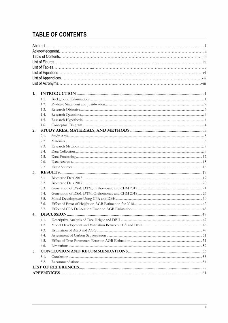
TABLE OF CONTENTS
Abstract………………………….………………………………………………………………………...i
Acknowledgment………………………………...…………………………..……………………………. ii
Table of Contents………………………………...…………………………...…...…………………...…. iii
List of Figures…………………………………..……………………………..…………………………. iv
List of Tables………………………..…………………………………………..…………………………v
List of Equations……………………………...………………………………………………………...…vi
List of Appendices………………………………..………………………………………………………vii
List of Acronyms…………………………………...………………………………………………….…viii
1. INTRODUCTION ........................................................................................................................................... 1
1.1. Background Information ...........................................................................................................................................1 1.2. Problem Statement and Justification ........................................................................................................................2 1.3. Research Objective ......................................................................................................................................................3 1.4. Research Questions .....................................................................................................................................................4 1.5. Research Hypothesis ...................................................................................................................................................4 1.6. Conceptual Diagram ...................................................................................................................................................4
2. STUDY AREA, MATERIALS, AND METHODS ................................................................................. 5
2.1. Study Area .....................................................................................................................................................................5 2.2. Materials ........................................................................................................................................................................6 2.3. Research Methods .......................................................................................................................................................7 2.4. Data Collection ............................................................................................................................................................9 2.5. Data Processing ........................................................................................................................................................ 12 2.6. Data Analysis ............................................................................................................................................................. 15 2.7. Error Sources ............................................................................................................................................................ 16
3. RESULTS .......................................................................................................................................................... 19
3.1. Biometric Data 2018 ................................................................................................................................................ 19 3.2. Biometric Data 2017 ................................................................................................................................................ 20 3.3. Generation of DSM, DTM, Orthomosaic and CHM 2017 .............................................................................. 21 3.4. Generation of DSM, DTM, Orthomosaic and CHM 2018 .............................................................................. 25 3.5. Model Development Using CPA and DBH ........................................................................................................ 30 3.6. Effect of Error of Height on AGB Estimation for 2018 .................................................................................. 42 3.7. Effect of CPA Delineation Error on AGB Estimation..................................................................................... 43
4. DISCUSSION .................................................................................................................................................. 47
4.1. Descriptive Analysis of Tree Height and DBH .................................................................................................. 47 4.2. Model Development and Validation Between CPA and DBH ....................................................................... 48 4.3. Estimation of AGB and AGC ............................................................................................................................... 49 4.4. Assessment of Carbon Sequestration ................................................................................................................... 51 4.5. Effect of Tree Parameters Error on AGB Estimation ...................................................................................... 51 4.6. Limitations ................................................................................................................................................................. 52
5. CONCLUSION AND RECOMMENDATIONS ................................................................................ 53
5.1. Conclusion ................................................................................................................................................................. 53 5.2. Recommendations .................................................................................................................................................... 54
LIST OF REFERENCES ..................................................................................................................................... 55
APPENDICES ......................................................................................................................................................... 61
iv
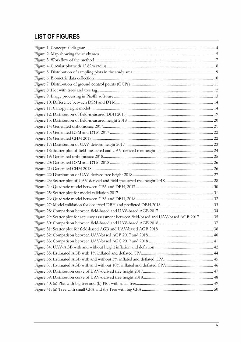
LIST OF FIGURES
Figure 1: Conceptual diagram ...................................................................................................................................... 4
Figure 2: Map showing the study area ........................................................................................................................ 5
Figure 3: Workflow of the method ............................................................................................................................. 7
Figure 4: Circular plot with 12.62m radius ................................................................................................................ 8
Figure 5: Distribution of sampling plots in the study area ...................................................................................... 9
Figure 6: Biometric data collection .......................................................................................................................... 10
Figure 7: Distribution of ground control points (GCPs) ..................................................................................... 11
Figure 8: Plot with trees and tree tag ....................................................................................................................... 12
Figure 9: Image processing in Pix4D software ...................................................................................................... 13
Figure 10: Difference between DSM and DTM .................................................................................................... 14
Figure 11: Canopy height model .............................................................................................................................. 14
Figure 12: Distribution of field-measured DBH 2018 ......................................................................................... 19
Figure 13: Distribution of field-measured height 2018 ........................................................................................ 20
Figure 14: Generated orthomosaic 2017................................................................................................................. 21
Figure 15: Generated DSM and DTM 2017 .......................................................................................................... 22
Figure 16: Generated CHM 2017............................................................................................................................. 22
Figure 17: Distribution of UAV-derived height 2017 .......................................................................................... 23
Figure 18: Scatter plot of field-measured and UAV-derived tree height ........................................................... 24
Figure 19: Generated orthomosaic 2018................................................................................................................. 25
Figure 20: Generated DSM and DTM 2018 .......................................................................................................... 26
Figure 21: Generated CHM 2018............................................................................................................................. 26
Figure 22: Distribution of UAV-derived tree height 2018 ................................................................................... 27
Figure 23: Scatter plot of UAV-derived and field-measured tree height 2018 ................................................. 28
Figure 24: Quadratic model between CPA and DBH, 2017 ............................................................................... 30
Figure 25: Scatter plot for model validation 2017 ................................................................................................. 31
Figure 26: Quadratic model between CPA and DBH, 2018 ............................................................................... 32
Figure 27: Model validation for observed DBH and predicted DBH 2018 ...................................................... 33
Figure 28: Comparison between field-based and UAV-based AGB 2017 ........................................................ 34
Figure 29: Scatter plot for accuracy assessment between field-based and UAV-based AGB 2017 .............. 35
Figure 30: Comparison between field-based and UAV-based AGB 2018 ........................................................ 37
Figure 31: Scatter plot for field-based AGB and UAV-based AGB 2018 ........................................................ 38
Figure 32: Comparison between UAV-based AGB 2017 and 2018 ................................................................... 40
Figure 33: Comparison between UAV-based AGC 2017 and 2018 .................................................................. 41
Figure 34: UAV-AGB with and without height inflation and deflation ............................................................ 42
Figure 35: Estimated AGB with 1% inflated and deflated CPA......................................................................... 44
Figure 36: Estimated AGB with and without 5% inflated and deflated CPA .................................................. 45
Figure 37: Estimated AGB with and without 10% inflated and deflated CPA ................................................ 46
Figure 38: Distribution curve of UAV-derived tree height 2017 ........................................................................ 47
Figure 39: Distribution curve of UAV-derived tree height 2018 ........................................................................ 48
Figure 40: (a) Plot with big tree and (b) Plot with small tree ............................................................................... 49
Figure 41: (a) Tree with small CPA and (b) Tree with big CPA ......................................................................... 50
v
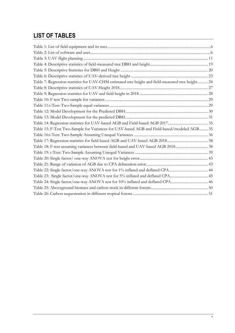
LIST OF TABLES
Table 1: List of field equipment and its uses ............................................................................................................. 6
Table 2: List of software and uses............................................................................................................................... 6
Table 3: UAV flight planning ................................................................................................................................... 11
Table 4: Descriptive statistics of field-measured tree DBH and height............................................................. 19
Table 5: Descriptive Statistics for DBH and Height ............................................................................................ 20
Table 6: Descriptive statistics of UAV-derived tree height ................................................................................. 23
Table 7: Regression statistics for UAV-CHM estimated tree height and field-measured tree height ........... 24
Table 8: Descriptive statistics of UAV Height 2018 ............................................................................................. 27
Table 9: Regression statistics for UAV and field height in 2018 ........................................................................ 28
Table 10: F-test Two-sample for variances ............................................................................................................ 29
Table 11:t-Test: Two-Sample equal variances ........................................................................................................ 29
Table 12: Model Development for the Predicted DBH ....................................................................................... 30
Table 13: Model Development for the predicted DBH ....................................................................................... 31
Table 14: Regression statistics for UAV-based AGB and Field-based AGB 2017 .......................................... 35
Table 15: F-Test Two-Sample for Variances for UAV-based AGB and Field-based/modeled AGB ......... 35
Table 16:t-Test: Two-Sample Assuming Unequal Variances .............................................................................. 36
Table 17: Regression statistics for field-based AGB and UAV-based AGB 2018 ........................................... 38
Table 18: F-test assuming variances between field-based and UAV-based AGB 2018 .................................. 38
Table 19: t-Test: Two-Sample Assuming Unequal Variances ............................................................................. 39
Table 20: Single factor/ one-way ANOVA test for height error ........................................................................ 43
Table 21: Range of variation of AGB due to CPA delineation error ................................................................. 43
Table 22: Single factor/one-way ANOVA test for 1% inflated and deflated CPA ......................................... 44
Table 23: Single factor/one-way ANOVA test for 5% inflated and deflated CPA........................................ 45
Table 24: Single factor/one-way ANOVA test for 10% inflated and deflated CPA....................................... 46
Table 25: Aboveground biomass and carbon stock in different forests ............................................................ 50
Table 26: Carbon sequestration in different tropical forests ............................................................................... 51
vi
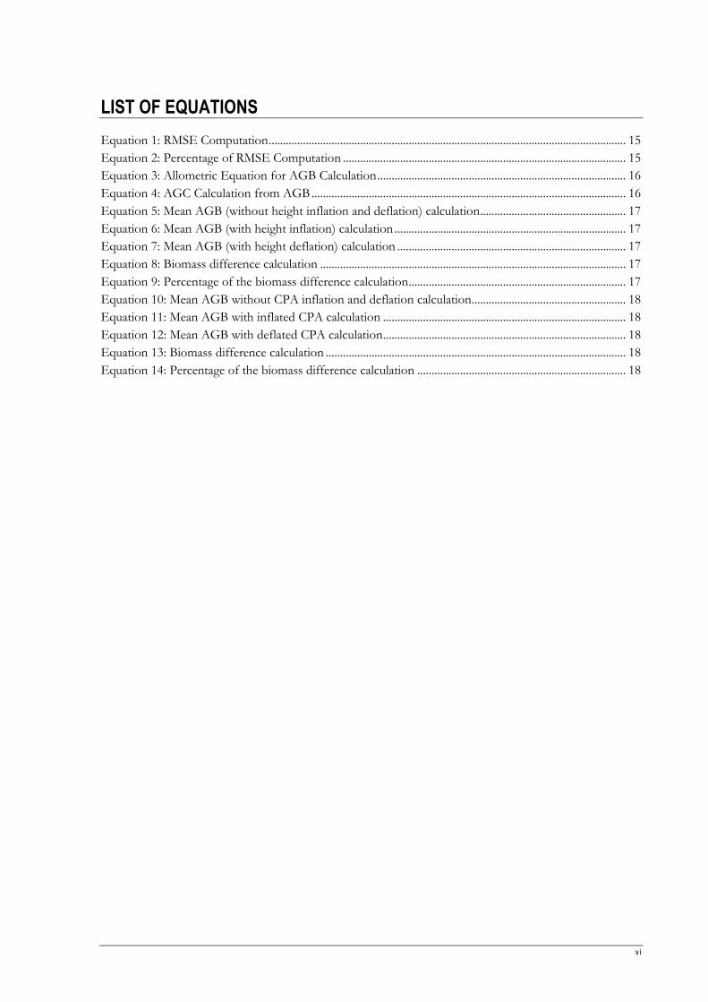
LIST OF EQUATIONS
Equation 1: RMSE Computation ............................................................................................................................. 15
Equation 2: Percentage of RMSE Computation ................................................................................................... 15
Equation 3: Allometric Equation for AGB Calculation ....................................................................................... 16
Equation 4: AGC Calculation from AGB .............................................................................................................. 16
Equation 5: Mean AGB (without height inflation and deflation) calculation ................................................... 17
Equation 6: Mean AGB (with height inflation) calculation ................................................................................. 17
Equation 7: Mean AGB (with height deflation) calculation ................................................................................ 17
Equation 8: Biomass difference calculation ........................................................................................................... 17
Equation 9: Percentage of the biomass difference calculation ............................................................................ 17
Equation 10: Mean AGB without CPA inflation and deflation calculation ...................................................... 18
Equation 11: Mean AGB with inflated CPA calculation ..................................................................................... 18
Equation 12: Mean AGB with deflated CPA calculation ..................................................................................... 18
Equation 13: Biomass difference calculation ......................................................................................................... 18
Equation 14: Percentage of the biomass difference calculation ......................................................................... 18

vii
LIST OF APPENDICES
Appendix 1: Biometric data collection sheet .......................................................................................................... 61
Appendix 2: Ground control point (GCP) marker ............................................................................................... 62
Appendix 3: Slope correction table ......................................................................................................................... 63
Appendix 4: Entry of biometric and UAV data in Microsoft Excel .................................................................. 64
Appendix 5: Comparison between field-based AGB/AGC and UAV-based AGB/AGC 2017 .................. 65
Appendix 6: Comparison between field-based AGB/AGC and UAV-based AGB/AGC 2018 .................. 66
viii
LIST OF ACRONYMS
AGB Aboveground biomass
AGC Aboveground carbon
ALS Airborne Laser Scanner
ANOVA Analysis of variance
CF Carbon Fraction
CHM Canopy Height Model
Cm Centimetre
CO2 Carbon dioxide
CP Check Point
CPA Crown projection area
DBH Diameter at Breast Height
DGPS Differential Global Positioning System
DSM Digital Surface Model
DTM Digital Terrain Model
GCP Ground Control Points
GHG Green House Gas
GIS Geographic Information System
GNSS Global Navigation Satellite System
GPS Global Positioning System
GSD Ground Sampling Distance
IMU Inertial Measurement Unit
IPCC Intergovernmental Panel on Climate Change
KRUS Kebun Raya UNMUL Samarinda
LiDAR Light Detection and Ranging
Mg Megagram
MT Missing Tree
MRV Monitoring, Reporting and Verifications
OBIA Object-Based Image Analysis
RADAR Radio Detection and Ranging
REDD+ Reducing Emissions from Deforestation and Forest Degradation
RMSE Root Mean Square Error
SfM Structure from Motion
TLS Terrestrial Laser Scanner
UAV Unmanned Aerial Vehicle
UNFCCC United Nations Framework Convention on Climate Change
UNMUL University of Mulawarman
2D Two Dimensional
3D Three Dimensional
ESTIMATION OF ABOVEGROUND BIOMASS/ CARBON STOCK AND CARBON SEQUESTRATION USING UAV IMAGERY AT KEBUN RAYA UNMUL SAMARINDA
EDUCATION FORESTS, EAST KALIMANTAN, INDONESIA
1
1. INTRODUCTION
1.1. Background Information
Environmental degradation from deforestation and forest degradation as well as land use change is one of
the major concerns for the global community because 17% of total greenhouse gas (GHG) are being
released from this source (IPCC, 2003). The importance of forests as both a sink and a source of greenhouse
gas emissions is globally recognized (Brown, 2002). Around 30% of the earth’s land surface is covered by
the forest while 45% of the total carbon is stored on land (Saatchi et al., 2011). Tropical rainforests have
been considered as one of the dominant types of forest that can play a crucial role in the context of
biodiversity conservation and climate change mitigation and adaptation. They can sequester and store more
carbon than any other forests (Gibbs et al., 2007). As stated by Saatchi et al. (2011) tropical forests can
sequester around 247 billion tons of carbon, of which 78.14% is sequestered in aboveground biomass while
the 21.86% of carbon is stored in belowground biomass. Tropical forests are recognized as the potential
sink of sequestering carbon from the atmosphere through protecting forested lands, slowing deforestation,
reforestation and agroforestry (Brown et al., 1996). However, deforestation and forest degradation occurred
in tropical forests due to natural and anthropogenic interventions (Ota et al., 2015). According to the
Intergovernmental Panel on Climate Change (IPCC), 1.6 billion tons of carbon are being released every
year, exclusively from deforestation and forest degradation (IPCC, 2003). The tropical forest located in
Southeast Asia contains 26% of the world’s tropical carbon, and unfortunately, this region is experiencing
more deforestation and forest degradation since 1990 (Saatchi et al., 2011). The climate change issue has
brought attention to the global community to protect the forest from deforestation and forest degradation,
specifically tropical forest. In 2005, UNFCCC commenced a process called “Reducing Emissions from
Deforestation and Forest Degradation, plus the role of conservation, sustainable management of forests
and enhancement of forest carbon stock (REDD+)” which is one of the key climate change mitigation
mechanism. Sustainable, consistent and robust monitoring, reporting and verification (MRVs) mechanism
should be operationalized to implement the REDD+ program successfully in every country. The estimation
of AGB and carbon stock is a prerequisite to achieving the objectives of REDD+ program and eventually,
to get the benefit from the newly emerging issue namely carbon trading.
Carbon stock is typically measured from the above ground biomass by assuming that half of the biomass is
carbon (Basuki et al., 2009). Cutting trees and weighing their different parts is the destructive method for
accurate estimation of biomass and carbon (Ebuy et al., 2011). This method is costly, labor-intensive and
time-consuming. This destructive method is supportive and helpful to develop allometric equations to assess
biomass and carbon stock (Clark et al., 2001). The forest parameters such as DBH, tree height, and wood
density are required as input in these allometric equations to estimate the forest aboveground biomass/
carbon stock (Basuki et al., 2009, Ketterings et al., 2001).
Remote sensing techniques are a better choice than field measurement for capturing the spatiotemporal
information of forest biophysical properties to assess biomass and carbon stock (Ota et al., 2017). Owing
to applications in the forestry sector, there are mainly three sources of remotely sensed data such as (i)
airborne laser scanning (ALS), (ii) radio detection and ranging (RADAR) (e.g., synthetic aperture radar), and
(iii) optical images (e.g., satellite or aerial images).
ESTIMATION OF ABOVEGROUND BIOMASS/ CARBON STOCK AND CARBON SEQUESTRATION USING UAV IMAGERY AT KEBUN RAYA UNMUL SAMARINDA
EDUCATION FORESTS, EAST KALIMANTAN, INDONESIA
2
The data acquisition using UAV-based platform has high operational flexibility in terms of cost, time,
platforms, place and repeatability compared to the satellite-based platform and traditional manned
photogrammetric operations (Stöcker et al., 2017). UAV has the capability of providing high spatial and
temporal resolution data which is useful in assessing AGB and carbon stock (Fritz et al., 2013). UAV
platform can capture high-resolution images that can be used effectively and efficiently to generate the digital
terrain model (DTM), digital surface model (DSM), and ortho-mosaic image (Stöcker et al., 2017).
The captured images from the UAV platform are used to generate DSM, DTM, and orthomosaic based on
structure from motion (SfM) technique. Structure from motion (SfM) represents the process to obtain a
three-dimensional structure of a scene of an object from a series of digital images (Micheletti et al., 2015).
SfM photogrammetry is cost and time-effective to estimate forest AGB and carbon stock. SfM uses a
sequence of overlapping images to produce a sparse 3D model of the scene. SfM photogrammetry approach
is capable of generating a digital surface model, reflecting the top of the canopy in the case of a forest and
a digital terrain model (Mlambo et al., 2017). Canopy height model (CHM) can be generated from DSM and
DTM. From CHM, the tree height can be extracted that would be the input for allometric equations to
assess biomass and carbon (Magar, 2014).
Among all biophysical parameters of the tree, diameter at breast height (DBH) is one of the essential
variables to assess the biomass and carbon because it explains more than 95% variation in biomass (Gibbs
et al., 2007). Studies have proved that there is a significant relationship between CPA and DBH (Anderson
et al., 2000). The correlation was demonstrated between CPA and all parts of trees such as foliage mass,
branch mass, stem mass for biomass (Kuuluvainen, 1991). The above ground biomass and carbon stock can
be assessed based on the relationship between CPA and DBH using regression model and allometric
equations (Basuki et al., 2009; Chave et al., 2005).
1.2. Problem Statement and Justification
Most of the studies on assessment of AGB/carbon stock and carbon sequestration in tropical rainforest has
been conducted using optical images (Du et al., 2012; Dube & Mutanga, 2015; Gibbs et al., 2007; Lu et al.,
2004; (Powell et al., 2010). The data collected from optical remote sensing can have problems due to clouds,
shadows, high saturation, low spectral variability, 2-D in nature and it is quite challenging to assess AGB
and carbon stock using these data (Kachamba et al., 2016). Although some medium-resolution remote
sensing data such as Landsat, Sentinel, etc. are freely available, it is difficult to use them to assess the forest
aboveground biomass and carbon stock due to pixel size, resolution versus tree crown size. Some very high-
resolution data such as QuickBird, IKONOS, etc. can estimate biomass accurately, but they are costly and
need highly technical knowledge to process. (Koh & Wich, 2012). The application of radar backscatter to
estimate AGB/carbon stock is challenging and leads to underestimation of AGB in the tropical forest
because of its high density and complex structure(Minh et al., 2014; Villard et al., 2016). L-band radar data
can be used to estimate AGB accurately up to 150 Mg ha-1 and it tends to saturate with AGB is greater than
150 Mg ha-1 (Villard et al., 2016). The decrease of intensity of radar backscatter also known as saturation
effect is the main reason for under-estimation of AGB (Minh et al., 2014). Recently, Lidar has proved to be
the best remote sensing technique to estimate biomass/ carbon stock accurately and precisely. However, it
is very expensive to assess biomass and carbon stock over a large area (Strahler et al., 2008). Unmanned
aerial vehicles (UAVs) can acquire high resolution remotely sensed data to estimate biomass and carbon
stock. The application of UAV is effective and efficient in assessing biomass with a relatively low cost for a
small area (Senthilnath et al., 2017). Furthermore, limited expertise is good enough to operate and acquire
data from the UAV platform.
ESTIMATION OF ABOVEGROUND BIOMASS/ CARBON STOCK AND CARBON SEQUESTRATION USING UAV IMAGERY AT KEBUN RAYA UNMUL SAMARINDA
EDUCATION FORESTS, EAST KALIMANTAN, INDONESIA
3
Conventional remote sensing techniques can provide horizontal forest structure accurately rather than
vertical forest structure. On the contrary, UAV is capable of providing horizontal and vertical forest
structure (Böttcher et al., 2009). In tropical rainforests, the estimation of above ground biomass and carbon
stock is quite challenging because of its complex stand structure and plentiful verities of species composition
(Nelson et al., 2000). A very limited number of researches were carried out using UAV images and Lidar in
a tropical forest. Clark et al. (2001) stated that the research on carbon flux and atmosphere is still insufficient
in a tropical forest. Based on that reason, it is essential to conduct research on quantifying and monitoring
carbon sequestration in a tropical forest. Few studies were carried out to estimate carbon sequestration
annually using high resolution remotely sensed data. The research on the accuracy of the assessment of the
AGB and carbon stock and specifically carbon sequestration using high-resolution UAV images of two
consecutive years would be helpful in the decision-making process to implement the REDD+ initiatives,
sustainable forest management and eventually natural resources management using its mechanism on MRV.
Despite having some benefits UAV also has limitations. The captured images by the UAV can only cover
the upper canopy of the tree. In the tropical forest, the lower canopy of trees is not visible because it is fully
or partially covered by the upper canopy trees. The point clouds are generated based on the captured images
that covered upper canopy, and it has an impact on assessing the total AGB and carbon stock. The different
sources of error or uncertainty have direct effects on AGB/ carbon stock and especially sequestration
estimation. The choice of remote sensing techniques influences the level of uncertainty in the estimate of
biomass (Gonzalez et al., 2010). The major sources of error in assessing AGB/carbon stock and carbon
sequestration are UAV data processing, tree parameter collection, allometric equations, ground-based
sampling, regression modeling. In a tropical forest, the measurement of height is challenging because of the
complex nature of the structure. It is quite challenging to extract accurate height form UAV-derived point
clouds. The height variation affects the total AGB/carbon stock estimation, and finally, it influences
assessing carbon sequestration. The variation of the amount of AGB and carbon stock of two years due to
height error might be affected more on carbon sequestration estimation. The manually delineated CPA or
automatic segmented CPA might have a certain level of inaccuracy, and it also has effects on biomass and
carbon sequestration estimation because the predicted DBH is found based on CPA. In order to have
complete and accurate biomass and carbon stock estimation, the identification and estimates of error are an
essential part of the process (Brown, 2002). Therefore, it is significant to identify and quantify these errors
and analyze the effect on biomass estimation and more specifically, how will that affect the carbon
sequestration.
1.3. Research Objective
General Objective
This study is aiming at the assessing of AGB/ carbon stock, carbon sequestration and evaluating the effects
of height and CPA delineation error on biomass estimation from very high-resolution UAV images based
on SfM photogrammetry approach at Kebun Raya UNMUL (University of Mulawarman) Samarinda
(KRUS) Education Forests, East Kalimantan, Indonesia.
Specific Objectives
1. To estimate the AGB/carbon stock of tropical rainforest for 2017 and 2018.
2. To assess the amount of sequestered carbon in the tropical forest for one year using UAV images.
3. To assess the accuracy of aboveground biomass of tropical rainforest estimated from UAV images.
4. To assess the effect of the error of tree parameters extracted from UAV images on AGB estimation.
ESTIMATION OF ABOVEGROUND BIOMASS/ CARBON STOCK AND CARBON SEQUESTRATION USING UAV IMAGERY AT KEBUN RAYA UNMUL SAMARINDA
EDUCATION FORESTS, EAST KALIMANTAN, INDONESIA
4
1.4. Research Questions
1. What is the estimated amount of the AGB/carbon stock for 2017 and 2018?
2. What is the estimated amount of sequestered carbon?
3. What is the accuracy of the aboveground biomass estimated from UAV images?
4. What is the error of UAV-derived tree height and how does that affect the AGB estimation?
5. How much the CPA delineation error affect the AGB estimation?
1.5. Research Hypothesis
1. Ho: There is no significant difference between estimated biomass from UAV imagery and field-
based biomass.
Ha: There is a significant difference between estimated biomass from UAV imagery and field-based
biomass.
2. Ho: The error of UAV-derived height has no significant influence on the AGB/ carbon estimation.
Ha: The error of UAV-derived height has a significant influence on the AGB/ carbon estimation.
3. Ho: The error of CPA delineation has no significant influence on the AGB/ carbon estimation.
Ha: The error of CPA delineation has a significant influence on the AGB/ carbon estimation.
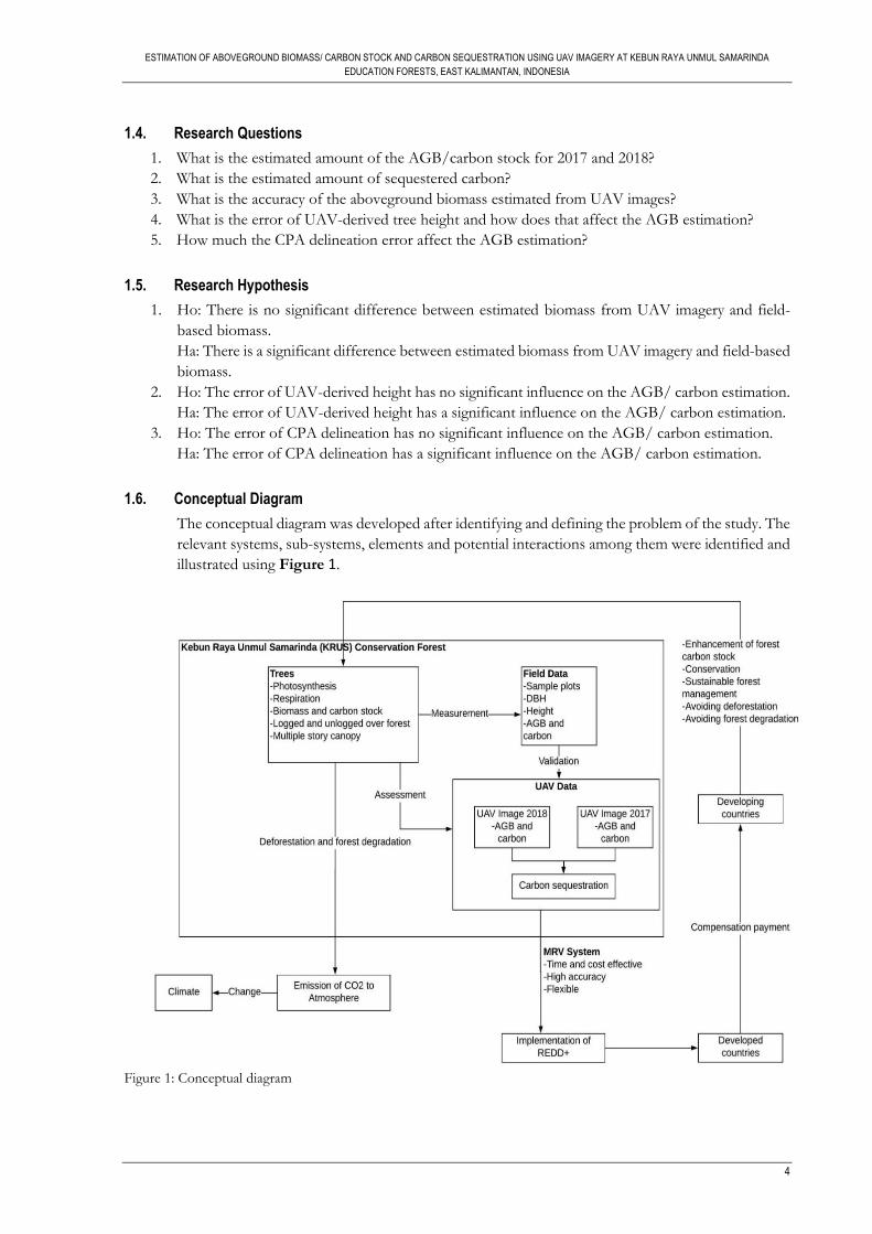
1.6. Conceptual Diagram
The conceptual diagram was developed after identifying and defining the problem of the study. The
relevant systems, sub-systems, elements and potential interactions among them were identified and
illustrated using Figure 1.
Figure 1: Conceptual diagram
ESTIMATION OF ABOVEGROUND BIOMASS/ CARBON STOCK AND CARBON SEQUESTRATION USING UAV IMAGERY AT KEBUN RAYA UNMUL SAMARINDA
EDUCATION FORESTS, EAST KALIMANTAN, INDONESIA
5
2. STUDY AREA, MATERIALS, AND METHODS
2.1. Study Area
UNMUL Samarinda botanical garden also known as ‘KRUS’ located in the Samarinda City of East
Kalimantan province, Indonesia which was belonging to CV. Mahakam wood before 1974. CV. Mahakam
wood handed over an area of 300 hectares to the rector of Mulawarman University in 1974. Then the area
was used as a conservation forest area and a suitable place for conducting research and educational activities
on tropical forest. On 9 July 1974, the area was inaugurated as educational forests. In 2001, 300 hectares
was reduced by 62 hectares because the area was allocated for a recreational botanical garden tourist spot
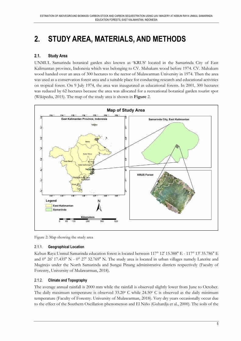
(Wikipedia, 2015). The map of the study area is shown in Figure 2.
Figure 2: Map showing the study area
Geographical Location
Kebun Raya Unmul Samarinda education forest is located between 117° 12' 15.388'' E - 117° 13' 35.786'' E
and 0° 26' 17.435'' N - 0° 27' 32.769'' N. The study area is located in urban villages namely Laterite and
Mugirejo under the North Samarinda and Sungai Pinang administrative districts respectively (Faculty of
Forestry, University of Mulawarman, 2018).
Climate and Topography
The average annual rainfall is 2000 mm while the rainfall is observed slightly lower from June to October.
The daily maximum temperature is observed 33.200 C while 24.500 C is observed as the daily minimum
temperature (Faculty of Forestry. University of Mulawarman, 2018). Very dry years occasionally occur due
to the effect of the Southern Oscillation phenomenon and El Niño (Guhardja et al., 2000). The soils of the
ESTIMATION OF ABOVEGROUND BIOMASS/ CARBON STOCK AND CARBON SEQUESTRATION USING UAV IMAGERY AT KEBUN RAYA UNMUL SAMARINDA
EDUCATION FORESTS, EAST KALIMANTAN, INDONESIA
6
study area are Podzolic Kandic, Podromolic Chromic, and Cambisol. The 60-70% of the study area consists
of forest areas with ramps up rather steep slope.
Vegetation
The study area is largely a forest area with vegetation cover logged secondary dry forest (logged-over areas),
and thickets with an area covering around 209 hectares while 29% of the area is the non-forested area.
Among the 70% of secondary forests, the dominant species are Artocarpus spp, Macaranga spp,
Eusideroxylon zwageri, Pentace spp, etc. (Faculty of Forestry. University of Mulawarman., 2018).
2.2. Materials
Field Equipment
The tools and equipment mentioned in Table 1 were used in the study to measure and collect the required
data from the field.
Table 1: List of field equipment and its uses
Name of tools/ equipment Uses
UAV Phanton4 DJI 2-D image capturing
Measuring tape (50m) Identification of the outer boundary of plots
Diameter tape (5m) Measurement of tree DBH
Handheld GPS (Garmin) Navigation and X, Y coordinate reading
Field data sheet and pencil Data recording
Range finder/ Haga altimeter Measurement of tree height
Leica DISTO D5 Height measurement
Tablet Navigation
Santo Clinometer Slope measurement
DGPS GCPs and plot center location
Data Processing Software
The different types of software were used to process and analyze the collected data from the study area. The
list of software and their uses are mentioned in
Table 2.
Table 2: List of software and uses
Name of software Uses
ArcMap 10.6.1 Data processing and visualization
Pix4D Photogrammetry processing
Erdas Imagine Resampling of ortho-mosaic image
Microsoft Excel Data analysis
Cloud compare 3-D point cloud visualization
Microsoft Word Reports and thesis writing
Mendeley Desktop Citation and references
Lucidchart Flowchart drawing
Microsoft power point Presentation of thesis
ESTIMATION OF ABOVEGROUND BIOMASS/ CARBON STOCK AND CARBON SEQUESTRATION USING UAV IMAGERY AT KEBUN RAYA UNMUL SAMARINDA
EDUCATION FORESTS, EAST KALIMANTAN, INDONESIA
7
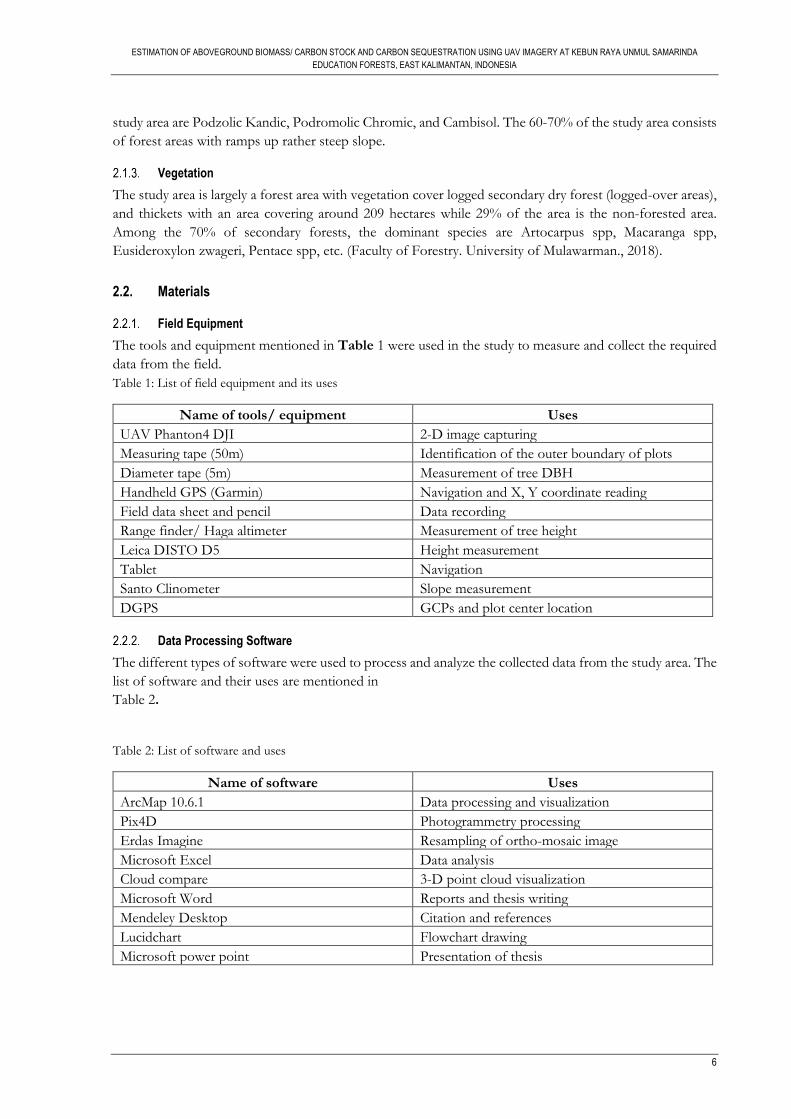
2.3. Research Methods
The research method encompasses the fieldwork design, spatial and statistical analysis and estimating the
AGB/AGC and carbon sequestration and lastly evaluating the influence of height and CPA delineation
error on assessing AGB. The research method of this study was comprised of five parts (see Figure 3):
(i) The first part was the biometric data collection, processing, and analysis. It involved the field
observation and acquiring required tree parameters using the above-mentioned instruments in
Table-1;
(ii) The second part was capturing digital images using a UAV platform. Then the data was
processed by Pix4D software to generate DSM, DTM and orthophoto;
(iii) The third part was the extraction of tree height from CHM generated from DSM and DTM;
(iv) In the fourth part, aboveground biomass (AGB)/ carbon stock and carbon sequestration were
assessed using tree height and predicted DBH extracted from UAV data in the third part.
(v) In the fifth and the last part, the effect of the height and CPA delineation error on aboveground
biomass was assessed.
Workflow of the Methods
Figure 3: Workflow of the method
ESTIMATION OF ABOVEGROUND BIOMASS/ CARBON STOCK AND CARBON SEQUESTRATION USING UAV IMAGERY AT KEBUN RAYA UNMUL SAMARINDA
EDUCATION FORESTS, EAST KALIMANTAN, INDONESIA
8
Pre-field Work
The pre-fieldwork activities such as preparing data collection sheet (see Appendix 1), black and white paint
marker and plastic tubes to set the ground control points (GCPs) (see Appendix 2), tree tag, testing of
equipment and tools to be used in the field, checking GPS and batteries condition of UAV were done before
going to field. Possible plots were identified in the orthomosaic images of 2017 and loaded in the tablet to
ease the identification of the plots as well as navigation.
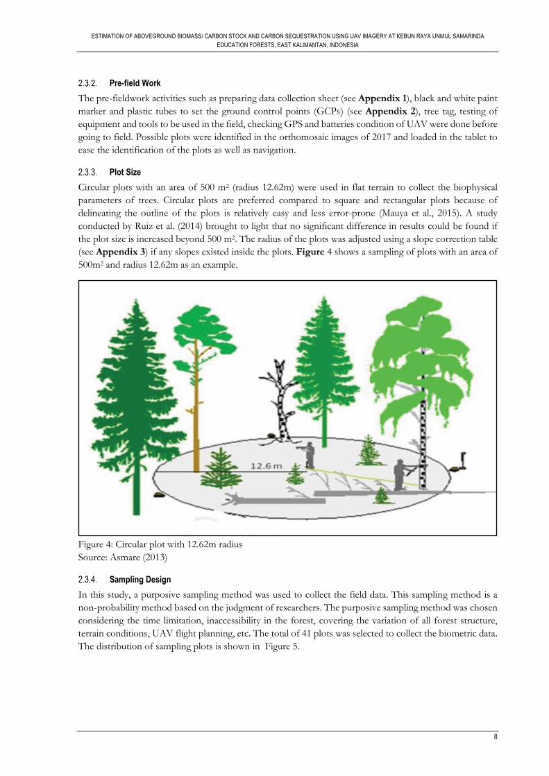
Plot Size
Circular plots with an area of 500 m2 (radius 12.62m) were used in flat terrain to collect the biophysical
parameters of trees. Circular plots are preferred compared to square and rectangular plots because of
delineating the outline of the plots is relatively easy and less error-prone (Mauya et al., 2015). A study
conducted by Ruiz et al. (2014) brought to light that no significant difference in results could be found if
the plot size is increased beyond 500 m2. The radius of the plots was adjusted using a slope correction table
(see Appendix 3) if any slopes existed inside the plots. Figure 4 shows a sampling of plots with an area of
500m2 and radius 12.62m as an example.
Figure 4: Circular plot with 12.62m radius
Source: Asmare (2013)
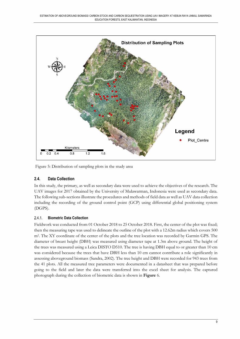
Sampling Design
In this study, a purposive sampling method was used to collect the field data. This sampling method is a
non-probability method based on the judgment of researchers. The purposive sampling method was chosen
considering the time limitation, inaccessibility in the forest, covering the variation of all forest structure,
terrain conditions, UAV flight planning, etc. The total of 41 plots was selected to collect the biometric data.
The distribution of sampling plots is shown in Figure 5.
ESTIMATION OF ABOVEGROUND BIOMASS/ CARBON STOCK AND CARBON SEQUESTRATION USING UAV IMAGERY AT KEBUN RAYA UNMUL SAMARINDA
EDUCATION FORESTS, EAST KALIMANTAN, INDONESIA
9
Figure 5: Distribution of sampling plots in the study area
2.4. Data Collection
In this study, the primary, as well as secondary data were used to achieve the objectives of the research. The
UAV images for 2017 obtained by the University of Mulawarman, Indonesia were used as secondary data.
The following sub-sections illustrate the procedures and methods of field data as well as UAV data collection
including the recording of the ground control point (GCP) using differential global positioning system
(DGPS).
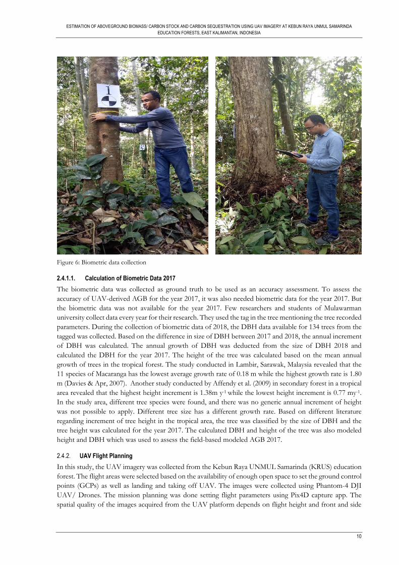
Biometric Data Collection
Fieldwork was conducted from 01 October 2018 to 25 October 2018. First, the center of the plot was fixed;
then the measuring tape was used to delineate the outline of the plot with a 12.62m radius which covers 500
m2. The XY coordinate of the center of the plots and the tree location was recorded by Garmin GPS. The
diameter of breast height (DBH) was measured using diameter tape at 1.3m above ground. The height of
the trees was measured using a Leica DISTO D510. The tree is having DBH equal to or greater than 10 cm
was considered because the trees that have DBH less than 10 cm cannot contribute a role significantly in
assessing aboveground biomass (Sandra, 2002). The tree height and DBH were recorded for 943 trees from
the 41 plots. All the measured tree parameters were documented in a datasheet that was prepared before
going to the field and later the data were transferred into the excel sheet for analysis. The captured
photograph during the collection of biometric data is shown in Figure 6.
ESTIMATION OF ABOVEGROUND BIOMASS/ CARBON STOCK AND CARBON SEQUESTRATION USING UAV IMAGERY AT KEBUN RAYA UNMUL SAMARINDA
EDUCATION FORESTS, EAST KALIMANTAN, INDONESIA
10
Figure 6: Biometric data collection
2.4.1.1. Calculation of Biometric Data 2017
The biometric data was collected as ground truth to be used as an accuracy assessment. To assess the
accuracy of UAV-derived AGB for the year 2017, it was also needed biometric data for the year 2017. But
the biometric data was not available for the year 2017. Few researchers and students of Mulawarman
university collect data every year for their research. They used the tag in the tree mentioning the tree recorded
parameters. During the collection of biometric data of 2018, the DBH data available for 134 trees from the
tagged was collected. Based on the difference in size of DBH between 2017 and 2018, the annual increment
of DBH was calculated. The annual growth of DBH was deducted from the size of DBH 2018 and
calculated the DBH for the year 2017. The height of the tree was calculated based on the mean annual
growth of trees in the tropical forest. The study conducted in Lambir, Sarawak, Malaysia revealed that the
11 species of Macaranga has the lowest average growth rate of 0.18 m while the highest growth rate is 1.80
m (Davies & Apr, 2007). Another study conducted by Affendy et al. (2009) in secondary forest in a tropical
area revealed that the highest height increment is 1.38m y-1 while the lowest height increment is 0.77 my-1.
In the study area, different tree species were found, and there was no generic annual increment of height
was not possible to apply. Different tree size has a different growth rate. Based on different literature
regarding increment of tree height in the tropical area, the tree was classified by the size of DBH and the
tree height was calculated for the year 2017. The calculated DBH and height of the tree was also modeled
height and DBH which was used to assess the field-based modeled AGB 2017.
UAV Flight Planning
In this study, the UAV imagery was collected from the Kebun Raya UNMUL Samarinda (KRUS) education
forest. The flight areas were selected based on the availability of enough open space to set the ground control
points (GCPs) as well as landing and taking off UAV. The images were collected using Phantom-4 DJI
UAV/ Drones. The mission planning was done setting flight parameters using Pix4D capture app. The
spatial quality of the images acquired from the UAV platform depends on flight height and front and side
ESTIMATION OF ABOVEGROUND BIOMASS/ CARBON STOCK AND CARBON SEQUESTRATION USING UAV IMAGERY AT KEBUN RAYA UNMUL SAMARINDA
EDUCATION FORESTS, EAST KALIMANTAN, INDONESIA
11
overlap. There is a significant relationship between flight height, overlap, weather conditions and the quality
of the point clouds (Dandois et al., 2015). Table 3 shows the image acquisition parameters that were set-up
to obtain the high-quality photogrammetric output.
Table 3: UAV flight planning
Parameter Value
Speed Moderate
Angle 900 (Nadir)
Front Overlap 75%
Side Overlap 65%
Flight Height 160 m -180 m
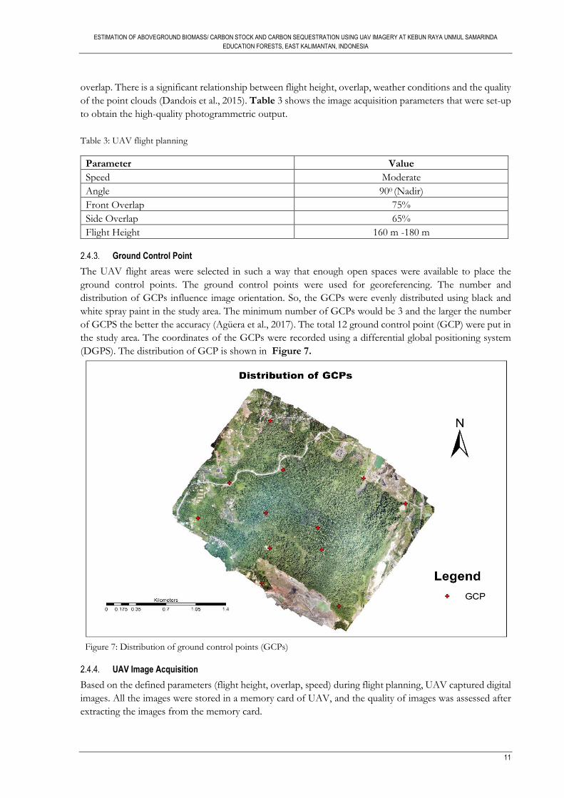
Ground Control Point
The UAV flight areas were selected in such a way that enough open spaces were available to place the
ground control points. The ground control points were used for georeferencing. The number and
distribution of GCPs influence image orientation. So, the GCPs were evenly distributed using black and
white spray paint in the study area. The minimum number of GCPs would be 3 and the larger the number
of GCPS the better the accuracy (Agüera et al., 2017). The total 12 ground control point (GCP) were put in
the study area. The coordinates of the GCPs were recorded using a differential global positioning system
(DGPS). The distribution of GCP is shown in Figure 7.
Figure 7: Distribution of ground control points (GCPs)
UAV Image Acquisition
Based on the defined parameters (flight height, overlap, speed) during flight planning, UAV captured digital
images. All the images were stored in a memory card of UAV, and the quality of images was assessed after
extracting the images from the memory card.
ESTIMATION OF ABOVEGROUND BIOMASS/ CARBON STOCK AND CARBON SEQUESTRATION USING UAV IMAGERY AT KEBUN RAYA UNMUL SAMARINDA
EDUCATION FORESTS, EAST KALIMANTAN, INDONESIA
12
2.5. Data Processing
The biometric and UAV data were processed after returning from the field using different types of software.
This section illustrates the procedures and methods of processing biometric data as well as UAV data.
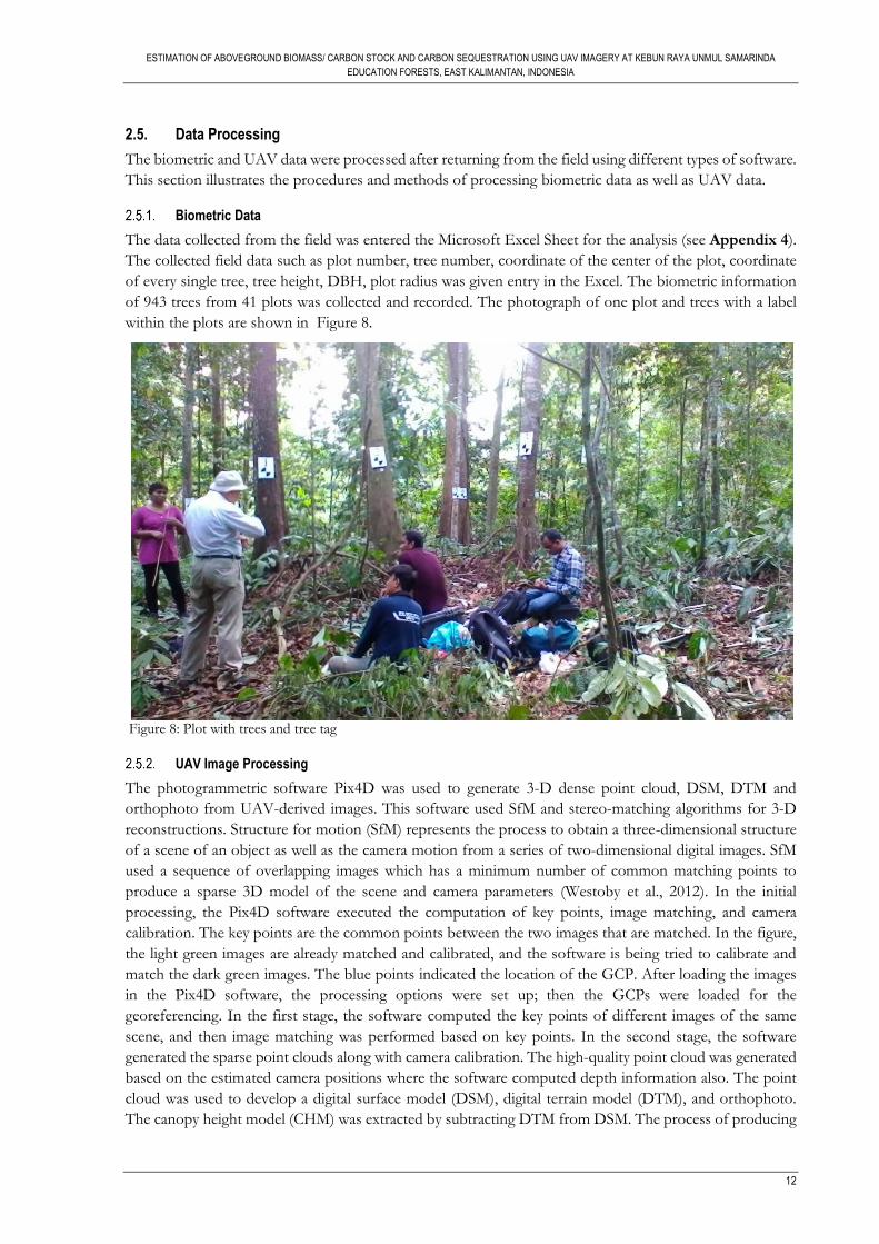
Biometric Data
The data collected from the field was entered the Microsoft Excel Sheet for the analysis (see Appendix 4).
The collected field data such as plot number, tree number, coordinate of the center of the plot, coordinate
of every single tree, tree height, DBH, plot radius was given entry in the Excel. The biometric information
of 943 trees from 41 plots was collected and recorded. The photograph of one plot and trees with a label
within the plots are shown in Figure 8.
Figure 8: Plot with trees and tree tag
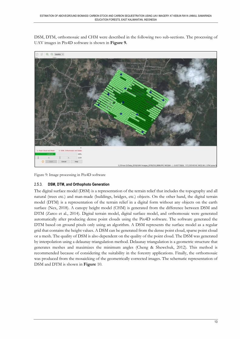
UAV Image Processing
The photogrammetric software Pix4D was used to generate 3-D dense point cloud, DSM, DTM and
orthophoto from UAV-derived images. This software used SfM and stereo-matching algorithms for 3-D
reconstructions. Structure for motion (SfM) represents the process to obtain a three-dimensional structure
of a scene of an object as well as the camera motion from a series of two-dimensional digital images. SfM
used a sequence of overlapping images which has a minimum number of common matching points to
produce a sparse 3D model of the scene and camera parameters (Westoby et al., 2012). In the initial
processing, the Pix4D software executed the computation of key points, image matching, and camera
calibration. The key points are the common points between the two images that are matched. In the figure,
the light green images are already matched and calibrated, and the software is being tried to calibrate and
match the dark green images. The blue points indicated the location of the GCP. After loading the images
in the Pix4D software, the processing options were set up; then the GCPs were loaded for the
georeferencing. In the first stage, the software computed the key points of different images of the same
scene, and then image matching was performed based on key points. In the second stage, the software
generated the sparse point clouds along with camera calibration. The high-quality point cloud was generated
based on the estimated camera positions where the software computed depth information also. The point
cloud was used to develop a digital surface model (DSM), digital terrain model (DTM), and orthophoto.
The canopy height model (CHM) was extracted by subtracting DTM from DSM. The process of producing
ESTIMATION OF ABOVEGROUND BIOMASS/ CARBON STOCK AND CARBON SEQUESTRATION USING UAV IMAGERY AT KEBUN RAYA UNMUL SAMARINDA
EDUCATION FORESTS, EAST KALIMANTAN, INDONESIA
13
DSM, DTM, orthomosaic and CHM were described in the following two sub-sections. The processing of
UAV images in Pix4D software is shown in Figure 9.
Figure 9: Image processing in Pix4D software
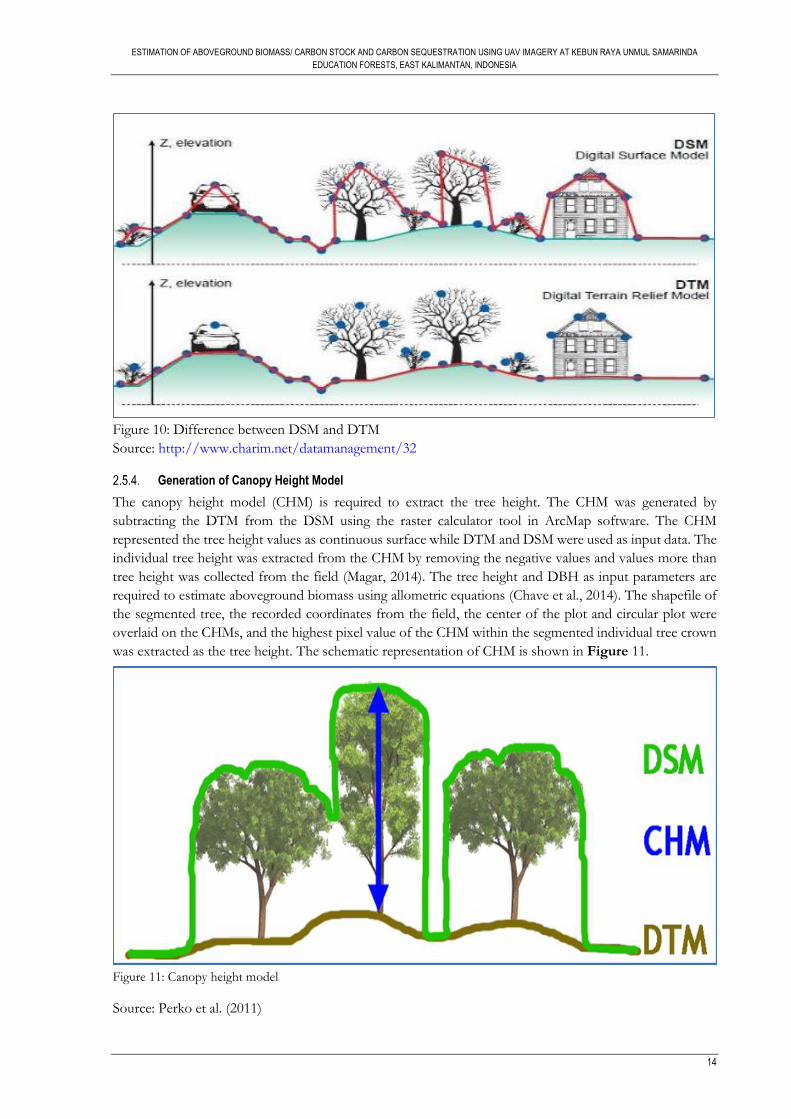
DSM, DTM, and Orthophoto Generation
The digital surface model (DSM) is a representation of the terrain relief that includes the topography and all
natural (trees etc.) and man-made (buildings, bridges, etc.) objects. On the other hand, the digital terrain
model (DTM) is a representation of the terrain relief in a digital form without any objects on the earth
surface (Nex, 2018). A canopy height model (CHM) is generated from the difference between DSM and
DTM (Zarco et al., 2014). Digital terrain model, digital surface model, and orthomosaic were generated
automatically after producing dense point clouds using the Pix4D software. The software generated the
DTM based on ground pixels only using an algorithm. A DSM represents the surface model as a regular
grid that contains the height values. A DSM can be generated from the dense point cloud, sparse point cloud
or a mesh. The quality of DSM is also dependent on the quality of the point cloud. The DSM was generated
by interpolation using a delaunay triangulation method. Delaunay triangulation is a geometric structure that
generates meshes and maximizes the minimum angles (Cheng & Shewchuk, 2012). This method is
recommended because of considering the suitability in the forestry applications. Finally, the orthomosaic
was produced from the mosaicking of the geometrically corrected images. The schematic representation of
DSM and DTM is shown in Figure 10.
ESTIMATION OF ABOVEGROUND BIOMASS/ CARBON STOCK AND CARBON SEQUESTRATION USING UAV IMAGERY AT KEBUN RAYA UNMUL SAMARINDA
EDUCATION FORESTS, EAST KALIMANTAN, INDONESIA
14
Figure 10: Difference between DSM and DTM
Source: http://www.charim.net/datamanagement/32
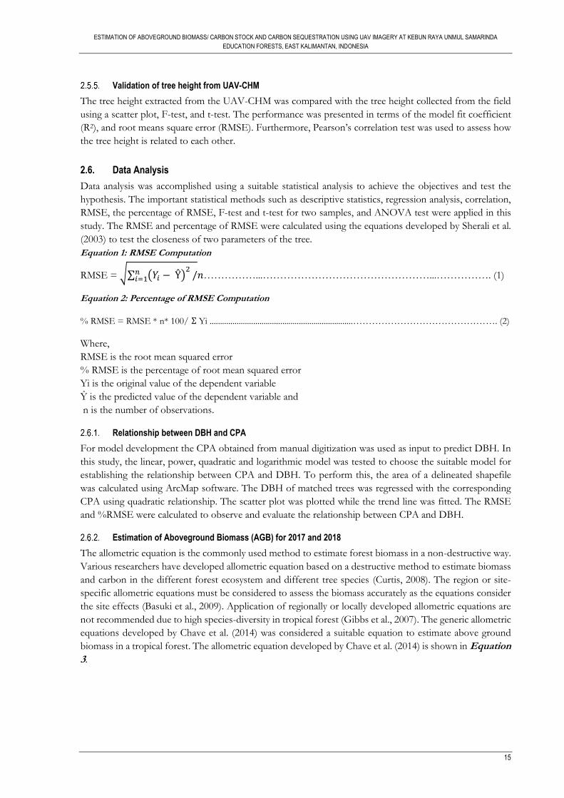
Generation of Canopy Height Model
The canopy height model (CHM) is required to extract the tree height. The CHM was generated by
subtracting the DTM from the DSM using the raster calculator tool in ArcMap software. The CHM
represented the tree height values as continuous surface while DTM and DSM were used as input data. The
individual tree height was extracted from the CHM by removing the negative values and values more than
tree height was collected from the field (Magar, 2014). The tree height and DBH as input parameters are
required to estimate aboveground biomass using allometric equations (Chave et al., 2014). The shapefile of
the segmented tree, the recorded coordinates from the field, the center of the plot and circular plot were
overlaid on the CHMs, and the highest pixel value of the CHM within the segmented individual tree crown
was extracted as the tree height. The schematic representation of CHM is shown in Figure 11.
Figure 11: Canopy height model
Source: Perko et al. (2011)
ESTIMATION OF ABOVEGROUND BIOMASS/ CARBON STOCK AND CARBON SEQUESTRATION USING UAV IMAGERY AT KEBUN RAYA UNMUL SAMARINDA
EDUCATION FORESTS, EAST KALIMANTAN, INDONESIA
15
Validation of tree height from UAV-CHM
The tree height extracted from the UAV-CHM was compared with the tree height collected from the field
using a scatter plot, F-test, and t-test. The performance was presented in terms of the model fit coefficient
(R2), and root means square error (RMSE). Furthermore, Pearson’s correlation test was used to assess how
the tree height is related to each other.
2.6. Data Analysis
Data analysis was accomplished using a suitable statistical analysis to achieve the objectives and test the
hypothesis. The important statistical methods such as descriptive statistics, regression analysis, correlation,
RMSE, the percentage of RMSE, F-test and t-test for two samples, and ANOVA test were applied in this
study. The RMSE and percentage of RMSE were calculated using the equations developed by Sherali et al.
(2003) to test the closeness of two parameters of the tree.
Equation 1: RMSE Computation
RMSE = √∑ (𝑌𝑖 − Ŷ)2𝑛
𝑖=1 /𝑛……………...…………………………………………...……………. (1)
Equation 2: Percentage of RMSE Computation
% RMSE = RMSE * n* 100/ Ʃ Yi .....................................................................………………………………………. (2)
Where,
RMSE is the root mean squared error
% RMSE is the percentage of root mean squared error
Yi is the original value of the dependent variable
Ŷ is the predicted value of the dependent variable and
n is the number of observations.
Relationship between DBH and CPA
For model development the CPA obtained from manual digitization was used as input to predict DBH. In
this study, the linear, power, quadratic and logarithmic model was tested to choose the suitable model for
establishing the relationship between CPA and DBH. To perform this, the area of a delineated shapefile
was calculated using ArcMap software. The DBH of matched trees was regressed with the corresponding
CPA using quadratic relationship. The scatter plot was plotted while the trend line was fitted. The RMSE
and %RMSE were calculated to observe and evaluate the relationship between CPA and DBH.
Estimation of Aboveground Biomass (AGB) for 2017 and 2018
The allometric equation is the commonly used method to estimate forest biomass in a non-destructive way.
Various researchers have developed allometric equation based on a destructive method to estimate biomass
and carbon in the different forest ecosystem and different tree species (Curtis, 2008). The region or site-
specific allometric equations must be considered to assess the biomass accurately as the equations consider
the site effects (Basuki et al., 2009). Application of regionally or locally developed allometric equations are
not recommended due to high species-diversity in tropical forest (Gibbs et al., 2007). The generic allometric
equations developed by Chave et al. (2014) was considered a suitable equation to estimate above ground
biomass in a tropical forest. The allometric equation developed by Chave et al. (2014) is shown in Equation
3.
ESTIMATION OF ABOVEGROUND BIOMASS/ CARBON STOCK AND CARBON SEQUESTRATION USING UAV IMAGERY AT KEBUN RAYA UNMUL SAMARINDA
EDUCATION FORESTS, EAST KALIMANTAN, INDONESIA
16
Equation 3: Allometric Equation for AGB Calculation
AGBest = 0.0673 × (ρD2 H)0.976…………………...……………………. (3) (Source: Chave et al., 2014)
Where AGBest is the estimated above ground biomass in kilograms (kg),
D is the diameter at breast height (DBH) in centimeter (cm),
H is the tree height in meter (m),
and ρ is wood density in gram per cubic centimeters (gcm-3),
0.0673 and 0.976 are constant.
The aboveground biomass (AGB) was estimated for the year 2017 and 2018 using this allometric equation.
The AGB was calculated and assessed for each plot.
Estimation of Aboveground Carbon for 2017 and 2018
The carbon stock was calculated from the estimated AGB. 50% of the estimated biomass is considered as
carbon (Houghton & Hackler, 2000; Burrows et al., 2002; & Drake et al., 2002). The carbon stock was
calculated using Equation 4.
.
Equation 4: AGC Calculation from AGB
AGC = AGB × CF…………………………………………………………………………………… (4)
Where,
AGC is aboveground carbon stock (Mg),
CF is the carbon fraction (0.5)
The total amount of sequestered carbon was assessed from the difference between the estimated amount of
carbon for 2017 and 2018.
Comparison of UAV-based AGB and Field-based AGB
The height derived from UAV-CHM and predicted DBH based on UAV CPA were used as an input
parameter to estimate the UAV-based AGB. The field-derived tree height and DBH were used as input
parameter for estimation of field-based AGB. The UAV-based AGB and Field-based AGB were compared
using a scatter plot and RMSE. Furthermore, the F-test and t-test were performed to test if there is a
significant difference between UAV-based AGB and Field-based AGB. Lastly, the mean difference between
the UAV-based AGB and Field-based AGB was assessed and evaluated.
2.7. Error Sources
Almost all related researches usually concentrate on accuracy assessment in each step they take in assessing
biomass and carbon stock and rarely consider the error propagation in final results carefully (Chave et al.,
2005). Error propagation assessment needs to be evaluated perfectly and properly to make correct
inferences. Measurement of error is expressed in terms of accuracy. It is essential to identify and assess the
influence of various sources of error on biomass and carbon estimation (Lo, 2005).
Main Sources of Error in AGB/ Carbon Estimation
The error and uncertainty originated from the multiple sources can influence the final biomass estimation
such as tree parameter measurement errors, errors in the allometric equation, data processing error, etc.
Chave et al. (2004) identified four types of error that could lead to statistical error in assessing biomass and
carbon: (i) tree measurement error; (ii) selection of allometric equations; (iii) choosing the size of the
sampling plot; (iv) landscape-scale representation. Nguyet (2012) stated five types of error namely: (i) field-
based carbon error; (ii) height extraction error; (iii) CPA extraction error; (iv) tree detection error; (v)
ESTIMATION OF ABOVEGROUND BIOMASS/ CARBON STOCK AND CARBON SEQUESTRATION USING UAV IMAGERY AT KEBUN RAYA UNMUL SAMARINDA
EDUCATION FORESTS, EAST KALIMANTAN, INDONESIA
17
classification error. Samalca (2007) identified two sources of uncertainty in his research like: (i) error in
selecting sampling plots (ii) selection of sampling trees. Holdaway et al. (2014) developed quantitative
statistical methods for propagating uncertainty in carbon estimation. They described the measurement error,
model uncertainty, and sampling uncertainty. Moreover, when assessing the sequestration of carbon
between two consecutive years, the error in measurement and assessed carbon sequestration might be
greater than the actual sequestration of carbon. There were very limited researches conducted on the
influence of height error and CPA delineation error on biomass and carbon estimation. In this research,
DBH and height were the input parameters for biomass assessment. For this reason, the effect of height
and CPA delineation error on AGB estimation was analyzed and discussed in this study.
2.7.1.1. Effects of Error of Height on AGB Estimation
The error of UAV-derived height is affected by the number of sources such as UAV quality data (point
density, seasonality), CHM generation process (interpolation algorithm), co-registration error, flight height,
number and distribution of GCPs. RMSE and percentage of RMSE of the estimated height were calculated
from the difference between height measurement from the field and height extracted from CHM. The height
derived from UAV-CHM was used to evaluate the variation of biomass due to the changes in height. How
much AGB is underestimated or overestimated was assessed by using height from the percentage of RMSE
calculated from UAV CHM height and field height for 2018. The single factor/ one-way ANOVA test was
performed to evaluate the significance of the difference between UAV-based AGB without inflated/
deflated height and the UAV-based AGB with inflated and deflated height for 2018. The influence of the
error of height on AGB estimation for the year 2017 was not analyzed because the biometric height for the
year 2017 was a modeled height calculated based on annual increment. It was assumed that the effect of the
error of height on AGB estimation would be the same. The percentage of error of estimated biomass was
assessed and analyzed based on calculating the percentage of the mean difference between original biomass
without inflation/deflation of height and the height inflated/deflated mean biomass values. The formula
for calculation of the average biomass is shown in Equations-5-9.
Equation 5: Mean AGB (without height inflation and deflation) calculation
Mean AGB (without height inflation and deflation) = {(ƩAGB of 41 plots)/Number of Plots} ………..………... (5)
Equation 6: Mean AGB (with height inflation) calculation
Mean AGB (with height inflation) = {(ƩAGB with height inflation of 41 plots)/Number of Plots} ………………(6)
Equation 7: Mean AGB (with height deflation) calculation
Mean AGB (with height deflation) = {(ƩAGB with height deflation of 41 plots)/Number of Plots} ..……...…… (7)
Equation 8: Biomass difference calculation
Biomass Difference = (Mean AGB with inflated height - Mean AGB with deflated height)/2.………...…………. (8)
Equation 9: Percentage of the biomass difference calculation
Percentage of Biomass Difference= {Biomass Difference/Mean AGB (without height inflation and deflation)}…….
×100…………………………………………………………………………………...…………………………. (9)
ESTIMATION OF ABOVEGROUND BIOMASS/ CARBON STOCK AND CARBON SEQUESTRATION USING UAV IMAGERY AT KEBUN RAYA UNMUL SAMARINDA
EDUCATION FORESTS, EAST KALIMANTAN, INDONESIA
18
2.7.1.2. Effects of CPA Delineation Error on AGB Estimation
The range of variation of biomass due to CPA delineation error was quantified and assessed by 1%, 5%,
and 10% inflated and deflated CPA delineation error. In this study, the CPA was delineated manually for
both years. It was assumed that the manually delineated CPA is more accurate and precise compared to the
automatic segmented CPA. However, due to the quality of orthomosaic and man-made error in visual
interpretation, the manually delineated CPA might have a certain level of inaccuracy. In this study, the
manually delineated CPA was inflated and deflated by 1%, 5%, and 10% and accordingly plot-based AGB
was calculated to evaluate the range of variation of biomass. After plot-based estimation of AGB with
inflated and deflated CPA, the range of variation of biomass was calculated based on Equations-10-14.
Equation 10: Mean AGB without CPA inflation and deflation calculation
Mean AGB (without CPA inflation and deflation) = {(ƩAGB of 41 plots)/Number of Plots} ………………... (10)
Equation 11: Mean AGB with inflated CPA calculation
Mean AGB (with CPA inflation) = {(ƩAGB with CPA inflation of 41 plots)/Number of Plots} ……..…………(11)
Equation 12: Mean AGB with deflated CPA calculation
Mean AGB (with CPA deflation) = {(ƩAGB with CPA deflation of 41 plots)/Number of Plot} ..……...……… (12)
Equation 13: Biomass difference calculation
Biomass Difference = (Mean AGB with inflated CPA - Mean AGB with deflated CPA)/2.…………….………. (13)
Equation 14: Percentage of the biomass difference calculation
Percentage of Biomass Difference= {Biomass Difference/Mean AGB (without CPA inflation and deflation)}……...
×100……………………………………………………………………………………………………………. (14)
ESTIMATION OF ABOVEGROUND BIOMASS/ CARBON STOCK AND CARBON SEQUESTRATION USING UAV IMAGERY AT KEBUN RAYA UNMUL SAMARINDA
EDUCATION FORESTS, EAST KALIMANTAN, INDONESIA
19
3. RESULTS
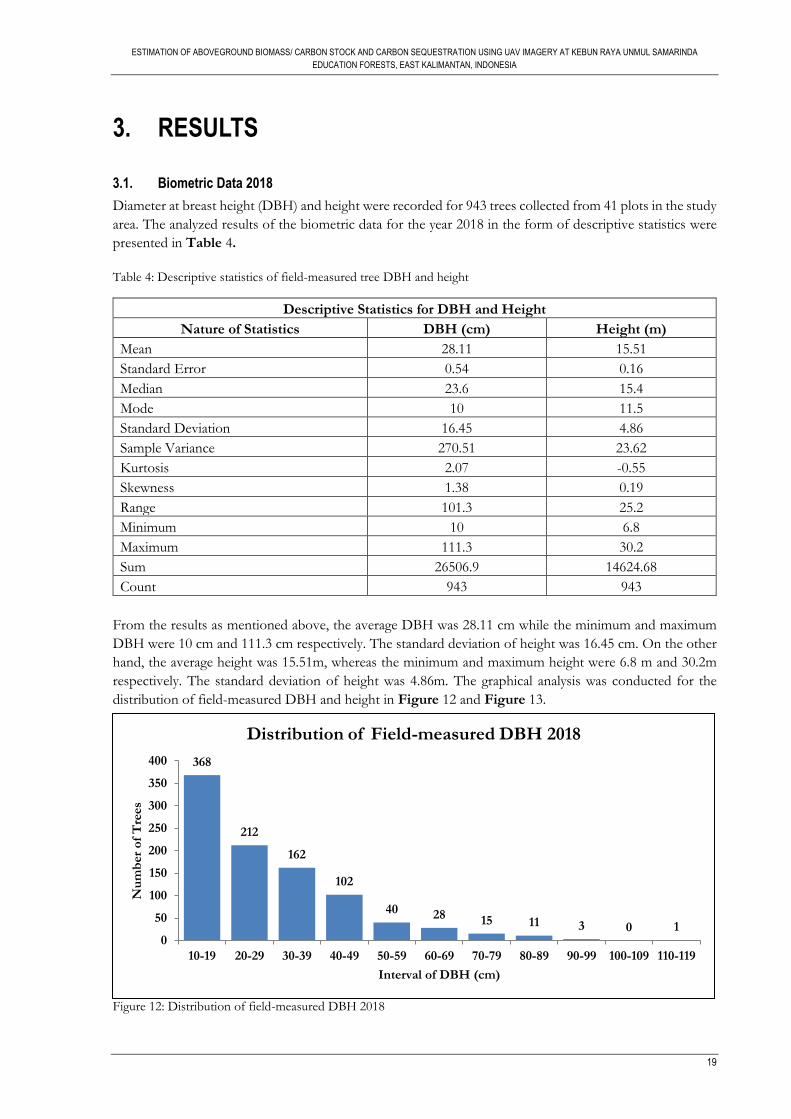
3.1. Biometric Data 2018
Diameter at breast height (DBH) and height were recorded for 943 trees collected from 41 plots in the study
area. The analyzed results of the biometric data for the year 2018 in the form of descriptive statistics were
presented in Table 4.
Table 4: Descriptive statistics of field-measured tree DBH and height
Descriptive Statistics for DBH and Height
Nature of Statistics DBH (cm) Height (m)
Mean 28.11 15.51
Standard Error 0.54 0.16
Median 23.6 15.4
Mode 10 11.5
Standard Deviation 16.45 4.86
Sample Variance 270.51 23.62
Kurtosis 2.07 -0.55
Skewness 1.38 0.19
Range 101.3 25.2
Minimum 10 6.8
Maximum 111.3 30.2
Sum 26506.9 14624.68
Count 943 943
From the results as mentioned above, the average DBH was 28.11 cm while the minimum and maximum
DBH were 10 cm and 111.3 cm respectively. The standard deviation of height was 16.45 cm. On the other
hand, the average height was 15.51m, whereas the minimum and maximum height were 6.8 m and 30.2m
respectively. The standard deviation of height was 4.86m. The graphical analysis was conducted for the
distribution of field-measured DBH and height in Figure 12 and Figure 13.
Figure 12: Distribution of field-measured DBH 2018
368
212
162
102
40 28 15 11 3 0 10
50
100
150
200
250
300
350
400
10-19 20-29 30-39 40-49 50-59 60-69 70-79 80-89 90-99 100-109 110-119
Nu
mb
er
of
Tre
es
Interval of DBH (cm)
Distribution of Field-measured DBH 2018
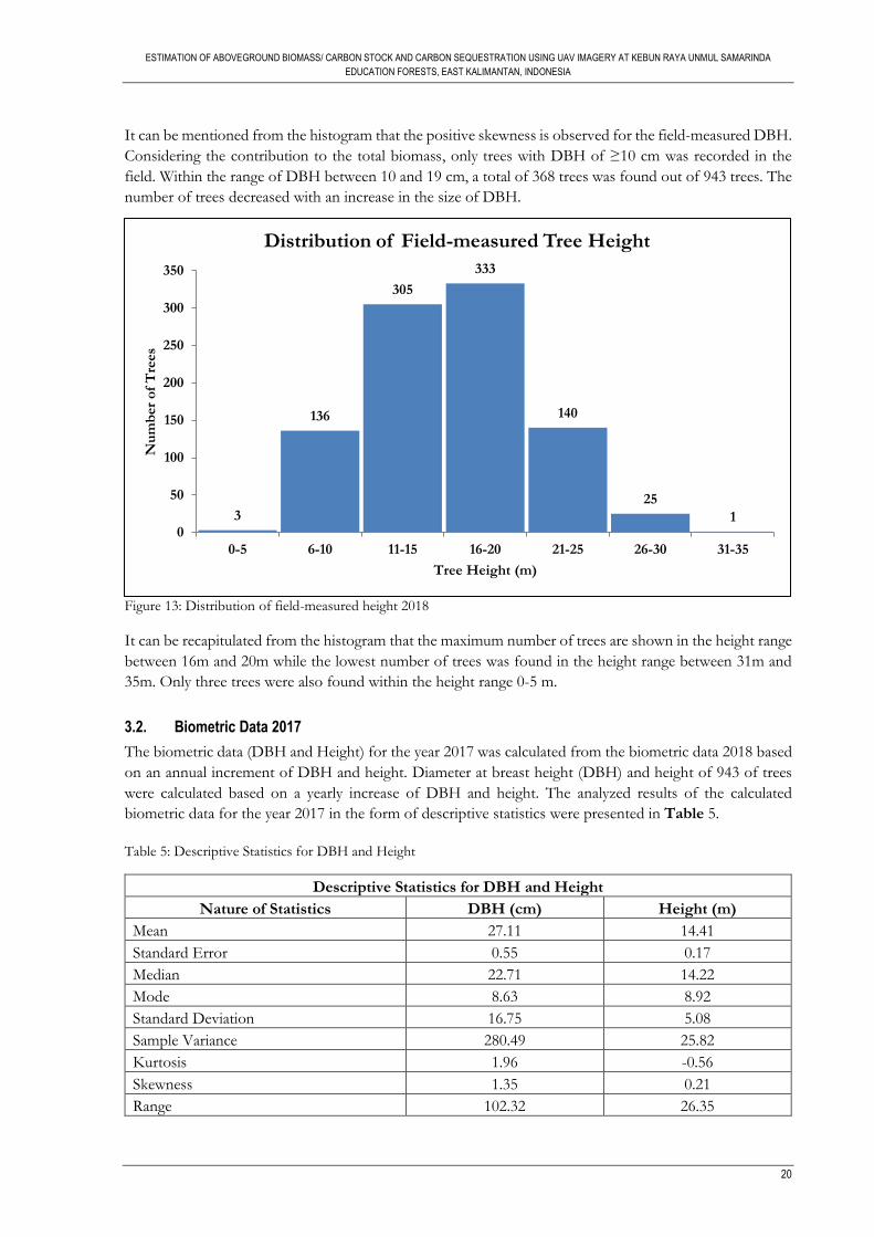
ESTIMATION OF ABOVEGROUND BIOMASS/ CARBON STOCK AND CARBON SEQUESTRATION USING UAV IMAGERY AT KEBUN RAYA UNMUL SAMARINDA
EDUCATION FORESTS, EAST KALIMANTAN, INDONESIA
20
It can be mentioned from the histogram that the positive skewness is observed for the field-measured DBH.
Considering the contribution to the total biomass, only trees with DBH of ≥10 cm was recorded in the
field. Within the range of DBH between 10 and 19 cm, a total of 368 trees was found out of 943 trees. The
number of trees decreased with an increase in the size of DBH.
Figure 13: Distribution of field-measured height 2018
It can be recapitulated from the histogram that the maximum number of trees are shown in the height range
between 16m and 20m while the lowest number of trees was found in the height range between 31m and
35m. Only three trees were also found within the height range 0-5 m.
3.2. Biometric Data 2017
The biometric data (DBH and Height) for the year 2017 was calculated from the biometric data 2018 based
on an annual increment of DBH and height. Diameter at breast height (DBH) and height of 943 of trees
were calculated based on a yearly increase of DBH and height. The analyzed results of the calculated
biometric data for the year 2017 in the form of descriptive statistics were presented in Table 5.
Table 5: Descriptive Statistics for DBH and Height
Descriptive Statistics for DBH and Height
Nature of Statistics DBH (cm) Height (m)
Mean 27.11 14.41
Standard Error 0.55 0.17
Median 22.71 14.22
Mode 8.63 8.92
Standard Deviation 16.75 5.08
Sample Variance 280.49 25.82
Kurtosis 1.96 -0.56
Skewness 1.35 0.21
Range 102.32 26.35
3
136
305
333
140
25
10
50
100
150
200
250
300
350
0-5 6-10 11-15 16-20 21-25 26-30 31-35
Nu
mb
er
of
Tre
es
Tree Height (m)
Distribution of Field-measured Tree Height
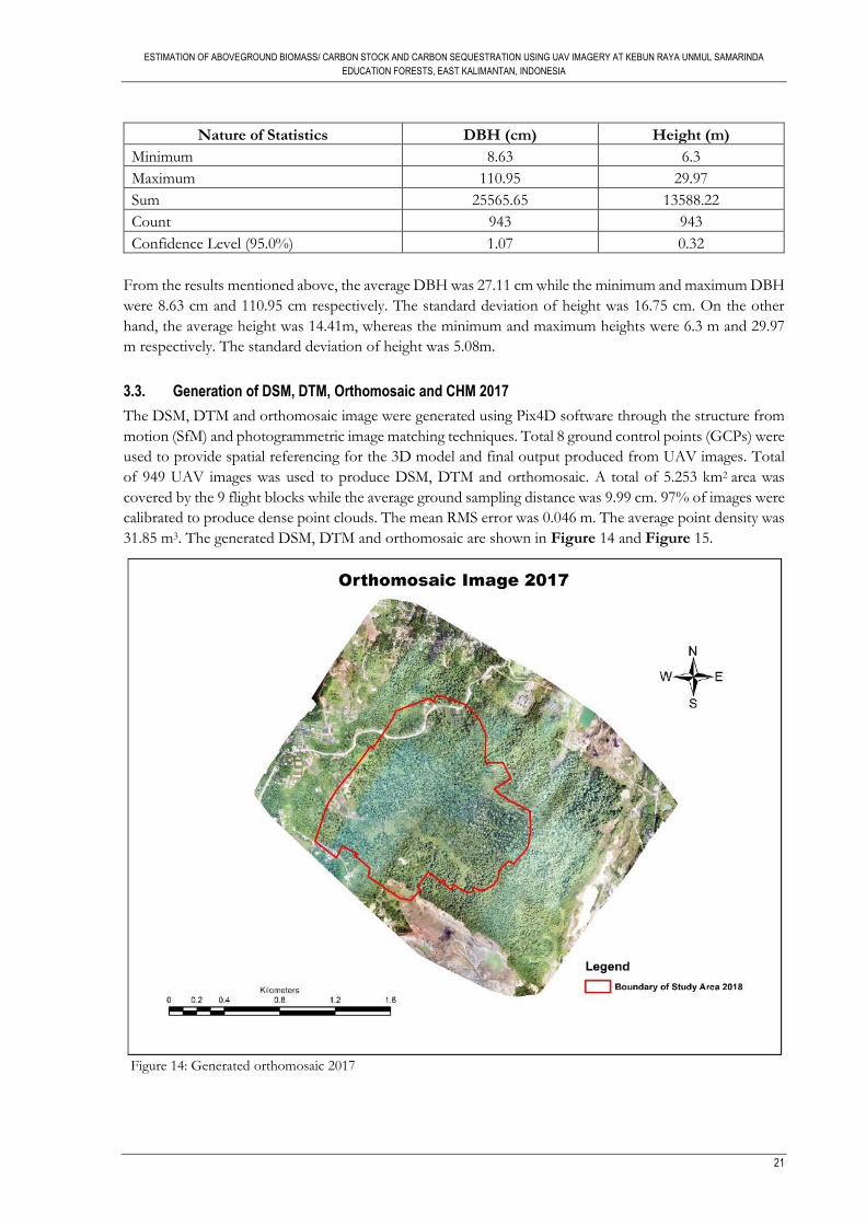
ESTIMATION OF ABOVEGROUND BIOMASS/ CARBON STOCK AND CARBON SEQUESTRATION USING UAV IMAGERY AT KEBUN RAYA UNMUL SAMARINDA
EDUCATION FORESTS, EAST KALIMANTAN, INDONESIA
21
Nature of Statistics DBH (cm) Height (m)
Minimum 8.63 6.3
Maximum 110.95 29.97
Sum 25565.65 13588.22
Count 943 943
Confidence Level (95.0%) 1.07 0.32
From the results mentioned above, the average DBH was 27.11 cm while the minimum and maximum DBH
were 8.63 cm and 110.95 cm respectively. The standard deviation of height was 16.75 cm. On the other
hand, the average height was 14.41m, whereas the minimum and maximum heights were 6.3 m and 29.97
m respectively. The standard deviation of height was 5.08m.
3.3. Generation of DSM, DTM, Orthomosaic and CHM 2017
The DSM, DTM and orthomosaic image were generated using Pix4D software through the structure from
motion (SfM) and photogrammetric image matching techniques. Total 8 ground control points (GCPs) were
used to provide spatial referencing for the 3D model and final output produced from UAV images. Total
of 949 UAV images was used to produce DSM, DTM and orthomosaic. A total of 5.253 km2 area was
covered by the 9 flight blocks while the average ground sampling distance was 9.99 cm. 97% of images were
calibrated to produce dense point clouds. The mean RMS error was 0.046 m. The average point density was
31.85 m3. The generated DSM, DTM and orthomosaic are shown in Figure 14 and Figure 15.
Figure 14: Generated orthomosaic 2017
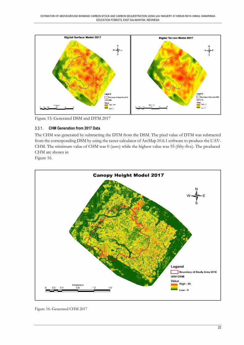
ESTIMATION OF ABOVEGROUND BIOMASS/ CARBON STOCK AND CARBON SEQUESTRATION USING UAV IMAGERY AT KEBUN RAYA UNMUL SAMARINDA
EDUCATION FORESTS, EAST KALIMANTAN, INDONESIA
22
Figure 15: Generated DSM and DTM 2017
CHM Generation from 2017 Data
The CHM was generated by subtracting the DTM from the DSM. The pixel value of DTM was subtracted
from the corresponding DSM by using the raster calculator of ArcMap 10.6.1 software to produce the UAV-
CHM. The minimum value of CHM was 0 (zero) while the highest value was 55 (fifty-five). The produced
CHM are shown in
Figure 16.
Figure 16: Generated CHM 2017
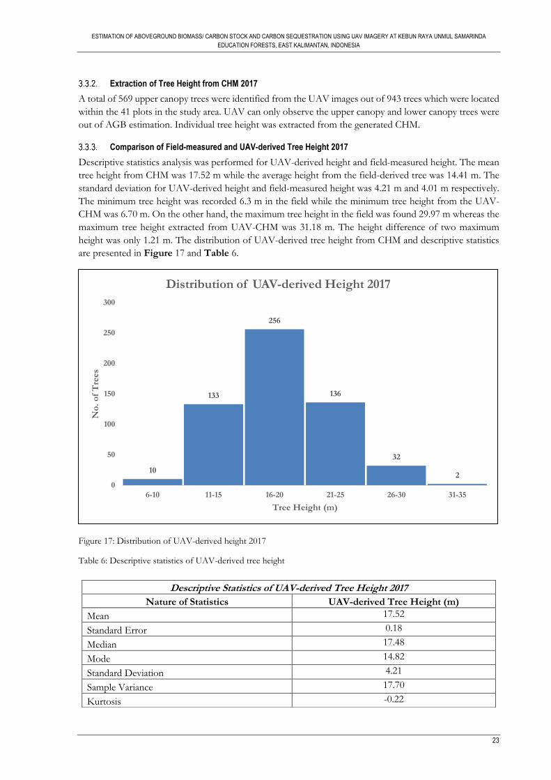
ESTIMATION OF ABOVEGROUND BIOMASS/ CARBON STOCK AND CARBON SEQUESTRATION USING UAV IMAGERY AT KEBUN RAYA UNMUL SAMARINDA
EDUCATION FORESTS, EAST KALIMANTAN, INDONESIA
23
Extraction of Tree Height from CHM 2017
A total of 569 upper canopy trees were identified from the UAV images out of 943 trees which were located
within the 41 plots in the study area. UAV can only observe the upper canopy and lower canopy trees were
out of AGB estimation. Individual tree height was extracted from the generated CHM.
Comparison of Field-measured and UAV-derived Tree Height 2017
Descriptive statistics analysis was performed for UAV-derived height and field-measured height. The mean
tree height from CHM was 17.52 m while the average height from the field-derived tree was 14.41 m. The
standard deviation for UAV-derived height and field-measured height was 4.21 m and 4.01 m respectively.
The minimum tree height was recorded 6.3 m in the field while the minimum tree height from the UAV-
CHM was 6.70 m. On the other hand, the maximum tree height in the field was found 29.97 m whereas the
maximum tree height extracted from UAV-CHM was 31.18 m. The height difference of two maximum
height was only 1.21 m. The distribution of UAV-derived tree height from CHM and descriptive statistics
are presented in Figure 17 and Table 6.
Figure 17: Distribution of UAV-derived height 2017
Table 6: Descriptive statistics of UAV-derived tree height
Descriptive Statistics of UAV-derived Tree Height 2017
Nature of Statistics UAV-derived Tree Height (m)
Mean 17.52
Standard Error 0.18
Median 17.48
Mode 14.82
Standard Deviation 4.21
Sample Variance 17.70
Kurtosis -0.22
10
133
256
136
32
2
0
50
100
150
200
250
300
6-10 11-15 16-20 21-25 26-30 31-35
No
. o
f T
rees
Tree Height (m)
Distribution of UAV-derived Height 2017
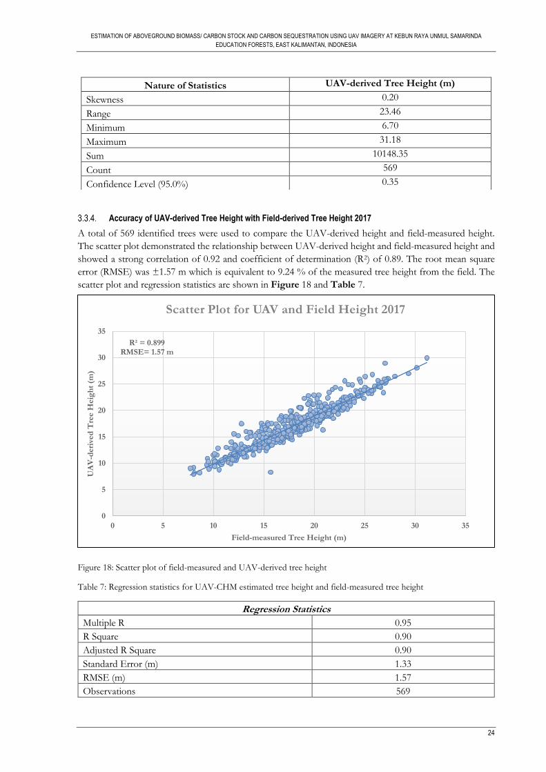
ESTIMATION OF ABOVEGROUND BIOMASS/ CARBON STOCK AND CARBON SEQUESTRATION USING UAV IMAGERY AT KEBUN RAYA UNMUL SAMARINDA
EDUCATION FORESTS, EAST KALIMANTAN, INDONESIA
24
Accuracy of UAV-derived Tree Height with Field-derived Tree Height 2017
A total of 569 identified trees were used to compare the UAV-derived height and field-measured height.
The scatter plot demonstrated the relationship between UAV-derived height and field-measured height and
showed a strong correlation of 0.92 and coefficient of determination (R2) of 0.89. The root mean square
error (RMSE) was ±1.57 m which is equivalent to 9.24 % of the measured tree height from the field. The
scatter plot and regression statistics are shown in Figure 18 and Table 7.
Figure 18: Scatter plot of field-measured and UAV-derived tree height
Table 7: Regression statistics for UAV-CHM estimated tree height and field-measured tree height
Regression Statistics
Multiple R 0.95
R Square 0.90
Adjusted R Square 0.90
Standard Error (m) 1.33
RMSE (m) 1.57
Observations 569
Nature of Statistics UAV-derived Tree Height (m)
Skewness 0.20
Range 23.46
Minimum 6.70
Maximum 31.18
Sum 10148.35
Count 569
Confidence Level (95.0%) 0.35
R² = 0.899RMSE= 1.57 m
0
5
10
15
20
25
30
35
0 5 10 15 20 25 30 35
UA
V-d
eri
ved
Tre
e H
eig
ht
(m)
Field-measured Tree Height (m)
Scatter Plot for UAV and Field Height 2017
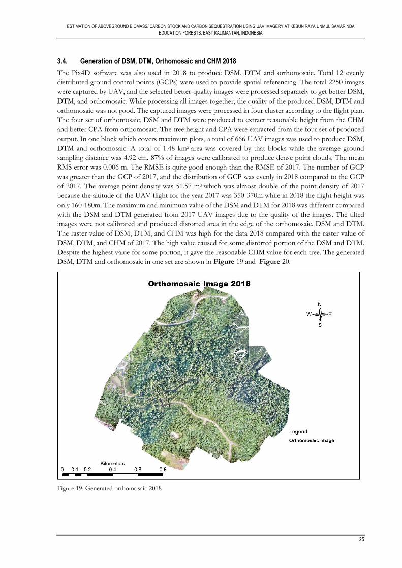
ESTIMATION OF ABOVEGROUND BIOMASS/ CARBON STOCK AND CARBON SEQUESTRATION USING UAV IMAGERY AT KEBUN RAYA UNMUL SAMARINDA
EDUCATION FORESTS, EAST KALIMANTAN, INDONESIA
25
3.4. Generation of DSM, DTM, Orthomosaic and CHM 2018
The Pix4D software was also used in 2018 to produce DSM, DTM and orthomosaic. Total 12 evenly
distributed ground control points (GCPs) were used to provide spatial referencing. The total 2250 images
were captured by UAV, and the selected better-quality images were processed separately to get better DSM,
DTM, and orthomosaic. While processing all images together, the quality of the produced DSM, DTM and
orthomosaic was not good. The captured images were processed in four cluster according to the flight plan.
The four set of orthomosaic, DSM and DTM were produced to extract reasonable height from the CHM
and better CPA from orthomosaic. The tree height and CPA were extracted from the four set of produced
output. In one block which covers maximum plots, a total of 666 UAV images was used to produce DSM,
DTM and orthomosaic. A total of 1.48 km2 area was covered by that blocks while the average ground
sampling distance was 4.92 cm. 87% of images were calibrated to produce dense point clouds. The mean
RMS error was 0.006 m. The RMSE is quite good enough than the RMSE of 2017. The number of GCP
was greater than the GCP of 2017, and the distribution of GCP was evenly in 2018 compared to the GCP
of 2017. The average point density was 51.57 m3 which was almost double of the point density of 2017
because the altitude of the UAV flight for the year 2017 was 350-370m while in 2018 the flight height was
only 160-180m. The maximum and minimum value of the DSM and DTM for 2018 was different compared
with the DSM and DTM generated from 2017 UAV images due to the quality of the images. The tilted
images were not calibrated and produced distorted area in the edge of the orthomosaic, DSM and DTM.
The raster value of DSM, DTM, and CHM was high for the data 2018 compared with the raster value of
DSM, DTM, and CHM of 2017. The high value caused for some distorted portion of the DSM and DTM.
Despite the highest value for some portion, it gave the reasonable CHM value for each tree. The generated
DSM, DTM and orthomosaic in one set are shown in Figure 19 and Figure 20.
Figure 19: Generated orthomosaic 2018
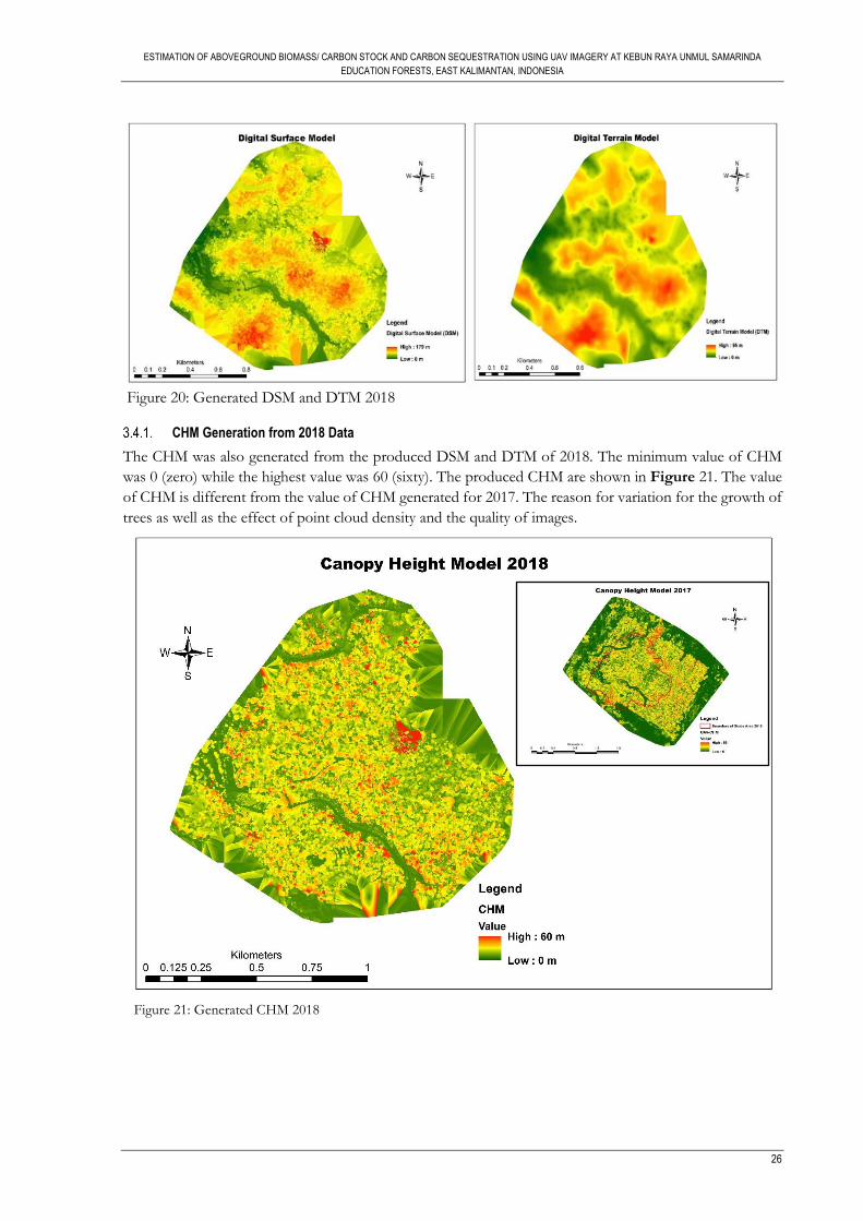
ESTIMATION OF ABOVEGROUND BIOMASS/ CARBON STOCK AND CARBON SEQUESTRATION USING UAV IMAGERY AT KEBUN RAYA UNMUL SAMARINDA
EDUCATION FORESTS, EAST KALIMANTAN, INDONESIA
26
Figure 20: Generated DSM and DTM 2018
CHM Generation from 2018 Data
The CHM was also generated from the produced DSM and DTM of 2018. The minimum value of CHM
was 0 (zero) while the highest value was 60 (sixty). The produced CHM are shown in Figure 21. The value
of CHM is different from the value of CHM generated for 2017. The reason for variation for the growth of
trees as well as the effect of point cloud density and the quality of images.
Figure 21: Generated CHM 2018
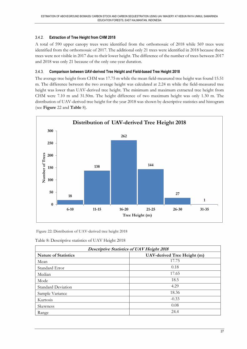
ESTIMATION OF ABOVEGROUND BIOMASS/ CARBON STOCK AND CARBON SEQUESTRATION USING UAV IMAGERY AT KEBUN RAYA UNMUL SAMARINDA
EDUCATION FORESTS, EAST KALIMANTAN, INDONESIA
27
Extraction of Tree Height from CHM 2018
A total of 590 upper canopy trees were identified from the orthomosaic of 2018 while 569 trees were
identified from the orthomosaic of 2017. The additional only 21 trees were identified in 2018 because these
trees were not visible in 2017 due to their lower height. The difference of the number of trees between 2017
and 2018 was only 21 because of the only one-year duration.
Comparison between UAV-derived Tree Height and Field-based Tree Height 2018
The average tree height from CHM was 17.75 m while the mean field-measured tree height was found 15.51
m. The difference between the two average height was calculated at 2.24 m while the field-measured tree
height was lower than UAV-derived tree height. The minimum and maximum extracted tree height from
CHM were 7.10 m and 31.50m. The height difference of two maximum height was only 1.30 m. The
distribution of UAV-derived tree height for the year 2018 was shown by descriptive statistics and histogram
(see Figure 22 and Table 8).
Figure 22: Distribution of UAV-derived tree height 2018
Table 8: Descriptive statistics of UAV Height 2018
Descriptive Statistics of UAV Height 2018
Nature of Statistics UAV-derived Tree Height (m)
Mean 17.75
Standard Error 0.18
Median 17.65
Mode 18.5
Standard Deviation 4.29
Sample Variance 18.36
Kurtosis -0.33
Skewness 0.08
Range 24.4
18
138
262
144
27
10
50
100
150
200
250
300
6-10 11-15 16-20 21-25 26-30 31-35
Nu
mb
er
of
Tre
es
Tree Height (m)
Distribution of UAV-derived Tree Height 2018
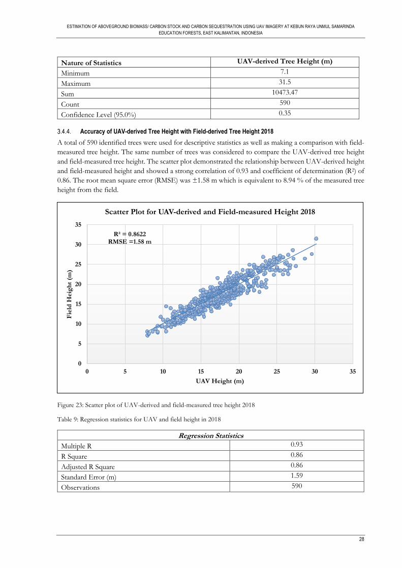
ESTIMATION OF ABOVEGROUND BIOMASS/ CARBON STOCK AND CARBON SEQUESTRATION USING UAV IMAGERY AT KEBUN RAYA UNMUL SAMARINDA
EDUCATION FORESTS, EAST KALIMANTAN, INDONESIA
28
Nature of Statistics UAV-derived Tree Height (m)
Minimum 7.1
Maximum 31.5
Sum 10473.47
Count 590
Confidence Level (95.0%) 0.35
Accuracy of UAV-derived Tree Height with Field-derived Tree Height 2018
A total of 590 identified trees were used for descriptive statistics as well as making a comparison with field-
measured tree height. The same number of trees was considered to compare the UAV-derived tree height
and field-measured tree height. The scatter plot demonstrated the relationship between UAV-derived height
and field-measured height and showed a strong correlation of 0.93 and coefficient of determination (R2) of
0.86. The root mean square error (RMSE) was ±1.58 m which is equivalent to 8.94 % of the measured tree
height from the field.
Figure 23: Scatter plot of UAV-derived and field-measured tree height 2018
Table 9: Regression statistics for UAV and field height in 2018
Regression Statistics
Multiple R 0.93
R Square 0.86
Adjusted R Square 0.86
Standard Error (m) 1.59
Observations 590
R² = 0.8622RMSE =1.58 m
0
5
10
15
20
25
30
35
0 5 10 15 20 25 30 35
Fie
ld H
eig
ht
(m)
UAV Height (m)
Scatter Plot for UAV-derived and Field-measured Height 2018
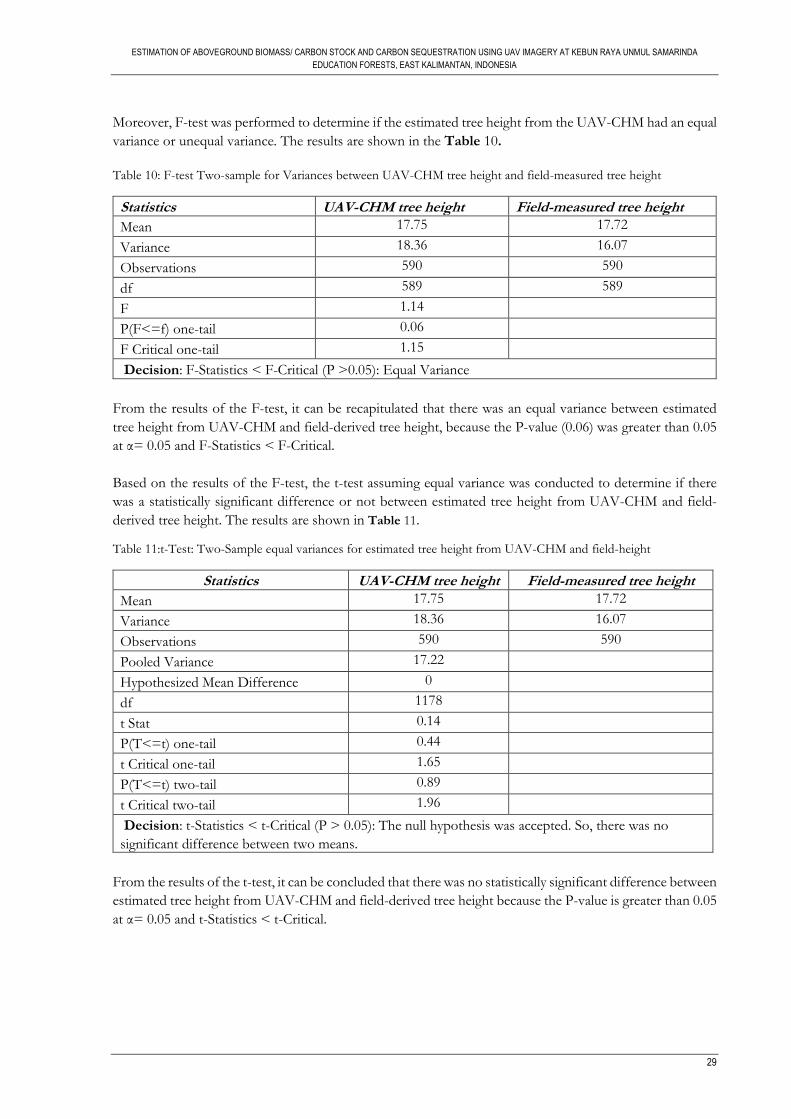
ESTIMATION OF ABOVEGROUND BIOMASS/ CARBON STOCK AND CARBON SEQUESTRATION USING UAV IMAGERY AT KEBUN RAYA UNMUL SAMARINDA
EDUCATION FORESTS, EAST KALIMANTAN, INDONESIA
29
Moreover, F-test was performed to determine if the estimated tree height from the UAV-CHM had an equal
variance or unequal variance. The results are shown in the Table 10.
Table 10: F-test Two-sample for Variances between UAV-CHM tree height and field-measured tree height
Statistics UAV-CHM tree height Field-measured tree height
Mean 17.75 17.72
Variance 18.36 16.07
Observations 590 590
df 589 589
F 1.14
P(F<=f) one-tail 0.06
F Critical one-tail 1.15
Decision: F-Statistics < F-Critical (P >0.05): Equal Variance
From the results of the F-test, it can be recapitulated that there was an equal variance between estimated
tree height from UAV-CHM and field-derived tree height, because the P-value (0.06) was greater than 0.05
at α= 0.05 and F-Statistics < F-Critical.
Based on the results of the F-test, the t-test assuming equal variance was conducted to determine if there
was a statistically significant difference or not between estimated tree height from UAV-CHM and field-
derived tree height. The results are shown in Table 11.
Table 11:t-Test: Two-Sample equal variances for estimated tree height from UAV-CHM and field-height
Statistics UAV-CHM tree height Field-measured tree height
Mean 17.75 17.72
Variance 18.36 16.07
Observations 590 590
Pooled Variance 17.22
Hypothesized Mean Difference 0
df 1178
t Stat 0.14
P(T<=t) one-tail 0.44
t Critical one-tail 1.65
P(T<=t) two-tail 0.89
t Critical two-tail 1.96
Decision: t-Statistics < t-Critical (P > 0.05): The null hypothesis was accepted. So, there was no
significant difference between two means.
From the results of the t-test, it can be concluded that there was no statistically significant difference between
estimated tree height from UAV-CHM and field-derived tree height because the P-value is greater than 0.05
at α= 0.05 and t-Statistics < t-Critical.
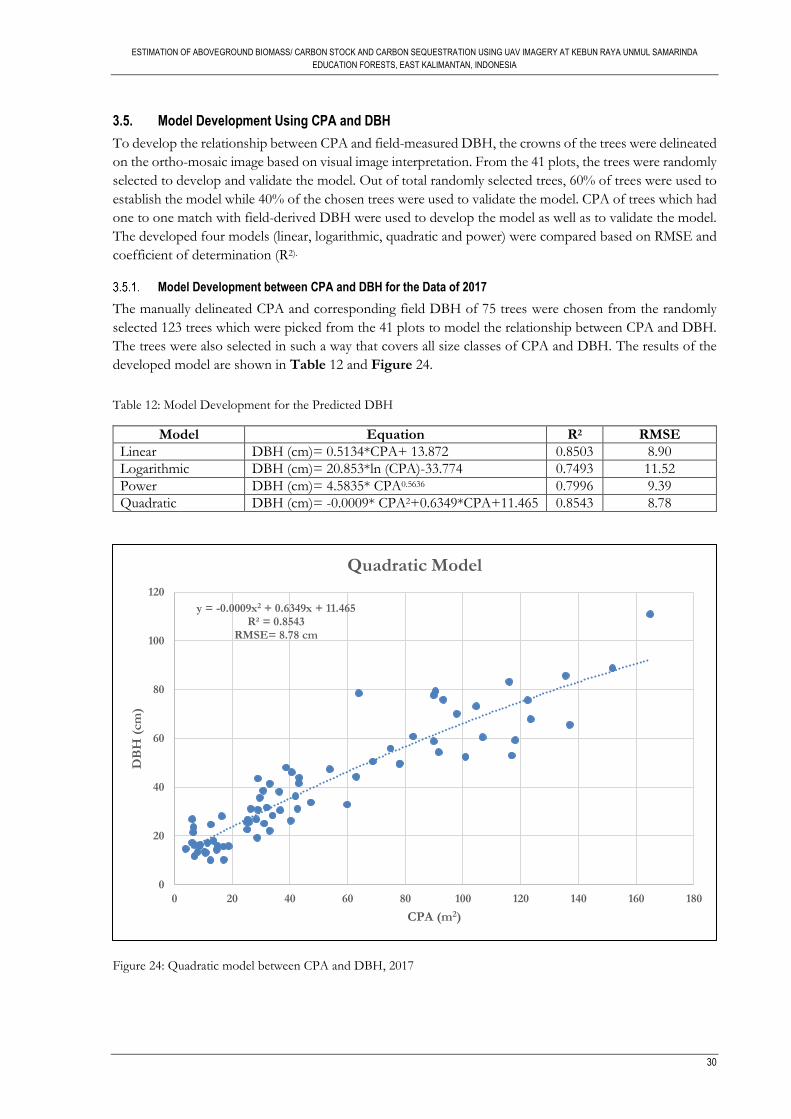
ESTIMATION OF ABOVEGROUND BIOMASS/ CARBON STOCK AND CARBON SEQUESTRATION USING UAV IMAGERY AT KEBUN RAYA UNMUL SAMARINDA
EDUCATION FORESTS, EAST KALIMANTAN, INDONESIA
30
3.5. Model Development Using CPA and DBH
To develop the relationship between CPA and field-measured DBH, the crowns of the trees were delineated
on the ortho-mosaic image based on visual image interpretation. From the 41 plots, the trees were randomly
selected to develop and validate the model. Out of total randomly selected trees, 60% of trees were used to
establish the model while 40% of the chosen trees were used to validate the model. CPA of trees which had
one to one match with field-derived DBH were used to develop the model as well as to validate the model.
The developed four models (linear, logarithmic, quadratic and power) were compared based on RMSE and
coefficient of determination (R2).
Model Development between CPA and DBH for the Data of 2017
The manually delineated CPA and corresponding field DBH of 75 trees were chosen from the randomly
selected 123 trees which were picked from the 41 plots to model the relationship between CPA and DBH.
The trees were also selected in such a way that covers all size classes of CPA and DBH. The results of the
developed model are shown in Table 12 and Figure 24.
Table 12: Model Development for the Predicted DBH
Model Equation R2 RMSE
Linear DBH (cm)= 0.5134*CPA+ 13.872 0.8503 8.90
Logarithmic DBH (cm)= 20.853*ln (CPA)-33.774 0.7493 11.52
Power DBH (cm)= 4.5835* CPA0.5636 0.7996 9.39
Quadratic DBH (cm)= -0.0009* CPA2+0.6349*CPA+11.465 0.8543 8.78
Figure 24: Quadratic model between CPA and DBH, 2017
y = -0.0009x2 + 0.6349x + 11.465R² = 0.8543
RMSE= 8.78 cm
0
20
40
60
80
100
120
0 20 40 60 80 100 120 140 160 180
DB
H (
cm
)
CPA (m2)
Quadratic Model
ESTIMATION OF ABOVEGROUND BIOMASS/ CARBON STOCK AND CARBON SEQUESTRATION USING UAV IMAGERY AT KEBUN RAYA UNMUL SAMARINDA
EDUCATION FORESTS, EAST KALIMANTAN, INDONESIA
31
From the results of the model development between CPA and DBH, it can be recapitulated that among all
models, the linear and quadratic models had the very nearest predictive power and errors. Among all models,
the quadratic model had the highest predictive power and the least errors. Considering the highest predictive
power and lowest RMSE, the quadratic model was selected for the prediction of DBH.
Model Validation for the Data 2017
The predicted DBH was validated using observed DBH by scatter plot. The model was validated using 48
(40% of selected trees) predicted and observed DBH those were chosen randomly from 123 trees from 41
plots. The value of the coefficient of determination (R2) was found at 0.89 (see Figure 25). The value of R2
means that 89% of the field DBH was explained by the quadratic model. The test of goodness of fit was
performed using RMSE that value was 8.22 cm.
Figure 25: Scatter plot for model validation 2017
Model Development between CPA and DBH for the Data 2018
The CPA and corresponding DBH of 70 trees were chosen from the randomly selected 123 trees from the
41 plots to model the relationship between CPA and DBH. The results of the developed model are shown
in the Table 13 and Figure 26.
Table 13: Model Development for the predicted DBH
Model Equation R2 RMSE
Linear DBH (cm)= 0.5263*CPA+ 15.669 0.7768 8.29
Logarithmic DBH (cm)= 18.693*ln (CPA)-27.037 0.7423 8.71
Power DBH (cm)= 4.9912* CPA0.5497 0.7339 8.03
Quadratic DBH (cm)= -0.0023* CPA2+0.7705*CPA+11.531 0.7872 8.05
R² = 0.8914
0
10
20
30
40
50
60
70
80
90
100
110
0 10 20 30 40 50 60 70 80 90 100
Pre
dic
ted
DB
H (
cm
)
Observed DBH (cm)
Model Validation for DBH
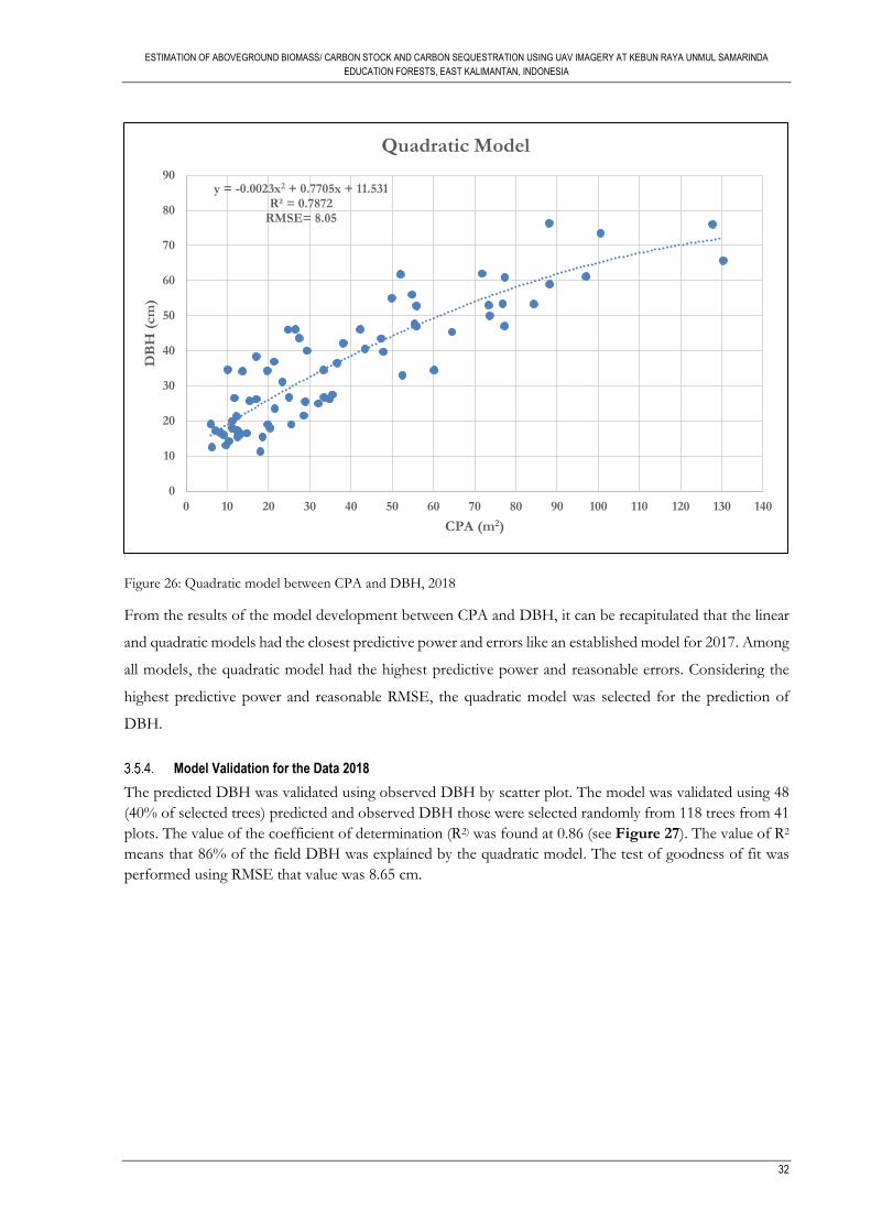
ESTIMATION OF ABOVEGROUND BIOMASS/ CARBON STOCK AND CARBON SEQUESTRATION USING UAV IMAGERY AT KEBUN RAYA UNMUL SAMARINDA
EDUCATION FORESTS, EAST KALIMANTAN, INDONESIA
32
[
Figure 26: Quadratic model between CPA and DBH, 2018
From the results of the model development between CPA and DBH, it can be recapitulated that the linear
and quadratic models had the closest predictive power and errors like an established model for 2017. Among
all models, the quadratic model had the highest predictive power and reasonable errors. Considering the
highest predictive power and reasonable RMSE, the quadratic model was selected for the prediction of
DBH.
Model Validation for the Data 2018
The predicted DBH was validated using observed DBH by scatter plot. The model was validated using 48
(40% of selected trees) predicted and observed DBH those were selected randomly from 118 trees from 41
plots. The value of the coefficient of determination (R2) was found at 0.86 (see Figure 27). The value of R2
means that 86% of the field DBH was explained by the quadratic model. The test of goodness of fit was
performed using RMSE that value was 8.65 cm.
y = -0.0023x2 + 0.7705x + 11.531R² = 0.7872
RMSE= 8.05
0
10
20
30
40
50
60
70
80
90
0 10 20 30 40 50 60 70 80 90 100 110 120 130 140
DB
H (
cm
)
CPA (m2)
Quadratic Model
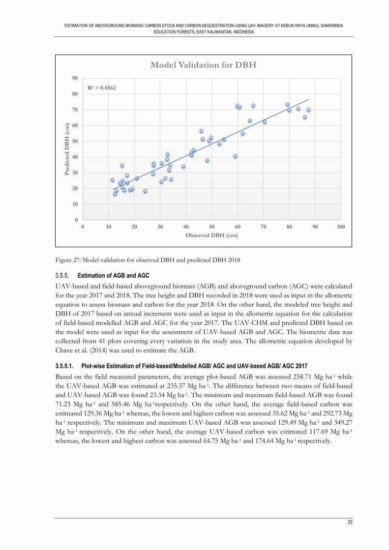
ESTIMATION OF ABOVEGROUND BIOMASS/ CARBON STOCK AND CARBON SEQUESTRATION USING UAV IMAGERY AT KEBUN RAYA UNMUL SAMARINDA
EDUCATION FORESTS, EAST KALIMANTAN, INDONESIA
33
Figure 27: Model validation for observed DBH and predicted DBH 2018
Estimation of AGB and AGC
UAV-based and field-based aboveground biomass (AGB) and aboveground carbon (AGC) were calculated
for the year 2017 and 2018. The tree height and DBH recorded in 2018 were used as input in the allometric
equation to assess biomass and carbon for the year 2018. On the other hand, the modeled tree height and
DBH of 2017 based on annual increment were used as input in the allometric equation for the calculation
of field-based modelled AGB and AGC for the year 2017. The UAV-CHM and predicted DBH based on
the model were used as input for the assessment of UAV-based AGB and AGC. The biometric data was
collected from 41 plots covering every variation in the study area. The allometric equation developed by
Chave et al. (2014) was used to estimate the AGB.
3.5.5.1. Plot-wise Estimation of Field-based/Modelled AGB/ AGC and UAV-based AGB/ AGC 2017
Based on the field measured parameters, the average plot-based AGB was assessed 258.71 Mg ha-1 while
the UAV-based AGB was estimated at 235.37 Mg ha-1. The difference between two means of field-based
and UAV-based AGB was found 23.34 Mg ha-1. The minimum and maximum field-based AGB was found
71.23 Mg ha-1 and 585.46 Mg ha-1respectively. On the other hand, the average field-based carbon was
estimated 129.36 Mg ha-1 whereas, the lowest and highest carbon was assessed 35.62 Mg ha-1 and 292.73 Mg
ha-1 respectively. The minimum and maximum UAV-based AGB was assessed 129.49 Mg ha-1 and 349.27
Mg ha-1 respectively. On the other hand, the average UAV-based carbon was estimated 117.69 Mg ha-1
whereas, the lowest and highest carbon was assessed 64.75 Mg ha-1 and 174.64 Mg ha-1 respectively.
R² = 0.8562
0
10
20
30
40
50
60
70
80
90
0 10 20 30 40 50 60 70 80 90 100
Pre
dic
ted
DB
H (
cm
)
Observed DBH (cm)
Model Validation for DBH
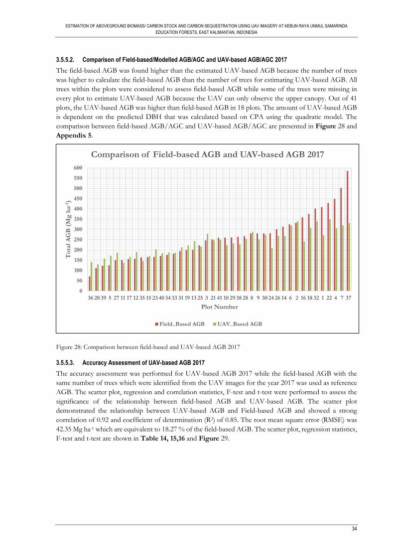
ESTIMATION OF ABOVEGROUND BIOMASS/ CARBON STOCK AND CARBON SEQUESTRATION USING UAV IMAGERY AT KEBUN RAYA UNMUL SAMARINDA
EDUCATION FORESTS, EAST KALIMANTAN, INDONESIA
34
3.5.5.2. Comparison of Field-based/Modelled AGB/AGC and UAV-based AGB/AGC 2017
The field-based AGB was found higher than the estimated UAV-based AGB because the number of trees
was higher to calculate the field-based AGB than the number of trees for estimating UAV-based AGB. All
trees within the plots were considered to assess field-based AGB while some of the trees were missing in
every plot to estimate UAV-based AGB because the UAV can only observe the upper canopy. Out of 41
plots, the UAV-based AGB was higher than field-based AGB in 18 plots. The amount of UAV-based AGB
is dependent on the predicted DBH that was calculated based on CPA using the quadratic model. The
comparison between field-based AGB/AGC and UAV-based AGB/AGC are presented in Figure 28 and
Appendix 5.
Figure 28: Comparison between field-based and UAV-based AGB 2017
3.5.5.3. Accuracy Assessment of UAV-based AGB 2017
The accuracy assessment was performed for UAV-based AGB 2017 while the field-based AGB with the
same number of trees which were identified from the UAV images for the year 2017 was used as reference
AGB. The scatter plot, regression and correlation statistics, F-test and t-test were performed to assess the
significance of the relationship between field-based AGB and UAV-based AGB. The scatter plot
demonstrated the relationship between UAV-based AGB and Field-based AGB and showed a strong
correlation of 0.92 and coefficient of determination (R2) of 0.85. The root mean square error (RMSE) was
42.35 Mg ha-1 which are equivalent to 18.27 % of the field-based AGB. The scatter plot, regression statistics,
F-test and t-test are shown in Table 14, 15,16 and Figure 29.
0
50
100
150
200
250
300
350
400
450
500
550
600
36 20 39 5 27 11 17 12 35 15 23 40 34 33 31 19 13 25 3 21 41 10 29 38 28 8 9 30 24 26 14 6 2 16 18 32 1 22 4 7 37
To
tal
AG
B (
Mg
ha
-1)
Plot Number
Comparison of Field-based AGB and UAV-based AGB 2017
Field_Based AGB UAV_Based AGB
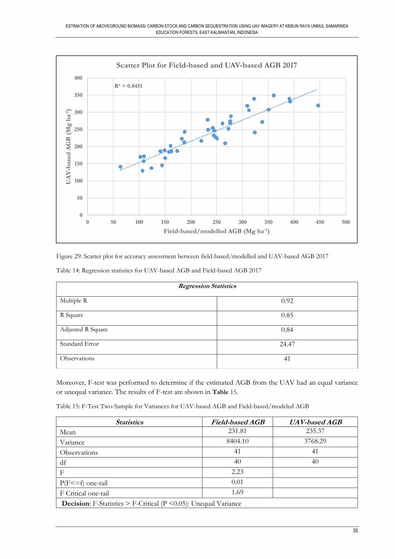
ESTIMATION OF ABOVEGROUND BIOMASS/ CARBON STOCK AND CARBON SEQUESTRATION USING UAV IMAGERY AT KEBUN RAYA UNMUL SAMARINDA
EDUCATION FORESTS, EAST KALIMANTAN, INDONESIA
35
Figure 29: Scatter plot for accuracy assessment between field-based/modelled and UAV-based AGB 2017
Table 14: Regression statistics for UAV-based AGB and Field-based AGB 2017
Moreover, F-test was performed to determine if the estimated AGB from the UAV had an equal variance
or unequal variance. The results of F-test are shown in Table 15.
Table 15: F-Test Two-Sample for Variances for UAV-based AGB and Field-based/modeled AGB
Statistics Field-based AGB UAV-based AGB
Mean 231.81 235.37
Variance 8404.10 3768.29
Observations 41 41
df 40 40
F 2.23
P(F<=f) one-tail 0.01
F Critical one-tail 1.69
Decision: F-Statistics > F-Critical (P <0.05): Unequal Variance
Regression Statistics
Multiple R 0.92
R Square 0.85
Adjusted R Square 0.84
Standard Error 24.47
Observations 41
R² = 0.8451
0
50
100
150
200
250
300
350
400
0 50 100 150 200 250 300 350 400 450 500
UA
V-b
ase
d A
GB
(M
g h
a-1)
Field-based/modelled AGB (Mg ha-1)
Scatter Plot for Field-based and UAV-based AGB 2017
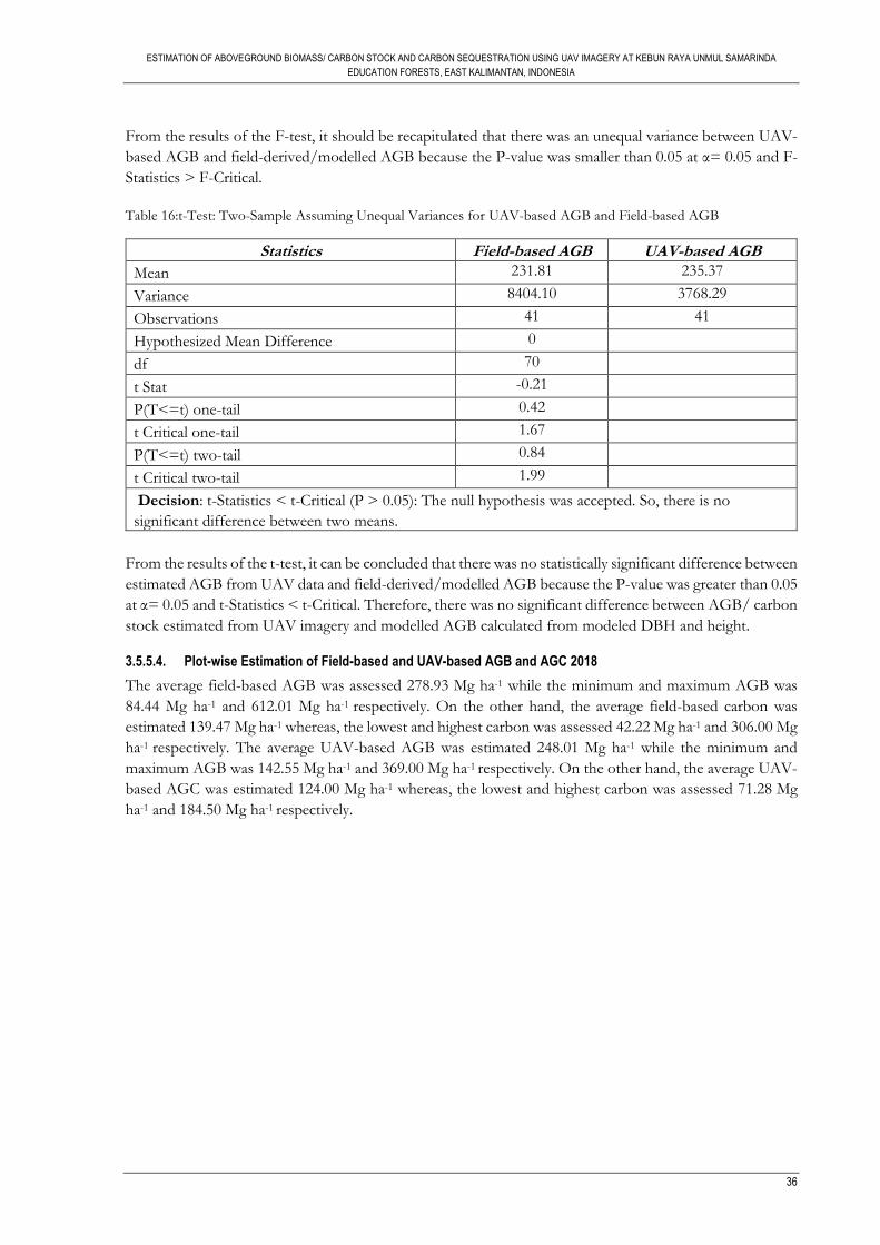
ESTIMATION OF ABOVEGROUND BIOMASS/ CARBON STOCK AND CARBON SEQUESTRATION USING UAV IMAGERY AT KEBUN RAYA UNMUL SAMARINDA
EDUCATION FORESTS, EAST KALIMANTAN, INDONESIA
36
From the results of the F-test, it should be recapitulated that there was an unequal variance between UAV-
based AGB and field-derived/modelled AGB because the P-value was smaller than 0.05 at α= 0.05 and F-
Statistics > F-Critical.
Table 16:t-Test: Two-Sample Assuming Unequal Variances for UAV-based AGB and Field-based AGB
Statistics Field-based AGB UAV-based AGB
Mean 231.81 235.37
Variance 8404.10 3768.29
Observations 41 41
Hypothesized Mean Difference 0
df 70
t Stat -0.21
P(T<=t) one-tail 0.42
t Critical one-tail 1.67
P(T<=t) two-tail 0.84
t Critical two-tail 1.99
Decision: t-Statistics < t-Critical (P > 0.05): The null hypothesis was accepted. So, there is no
significant difference between two means.
From the results of the t-test, it can be concluded that there was no statistically significant difference between
estimated AGB from UAV data and field-derived/modelled AGB because the P-value was greater than 0.05
at α= 0.05 and t-Statistics < t-Critical. Therefore, there was no significant difference between AGB/ carbon
stock estimated from UAV imagery and modelled AGB calculated from modeled DBH and height.
3.5.5.4. Plot-wise Estimation of Field-based and UAV-based AGB and AGC 2018
The average field-based AGB was assessed 278.93 Mg ha-1 while the minimum and maximum AGB was
84.44 Mg ha-1 and 612.01 Mg ha-1 respectively. On the other hand, the average field-based carbon was
estimated 139.47 Mg ha-1 whereas, the lowest and highest carbon was assessed 42.22 Mg ha-1 and 306.00 Mg
ha-1 respectively. The average UAV-based AGB was estimated 248.01 Mg ha-1 while the minimum and
maximum AGB was 142.55 Mg ha-1 and 369.00 Mg ha-1 respectively. On the other hand, the average UAV-
based AGC was estimated 124.00 Mg ha-1 whereas, the lowest and highest carbon was assessed 71.28 Mg
ha-1 and 184.50 Mg ha-1 respectively.
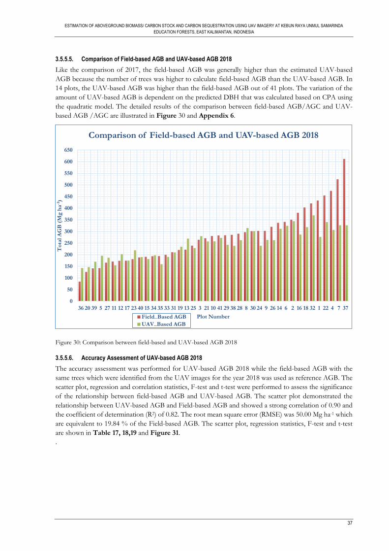
ESTIMATION OF ABOVEGROUND BIOMASS/ CARBON STOCK AND CARBON SEQUESTRATION USING UAV IMAGERY AT KEBUN RAYA UNMUL SAMARINDA
EDUCATION FORESTS, EAST KALIMANTAN, INDONESIA
37
3.5.5.5. Comparison of Field-based AGB and UAV-based AGB 2018
Like the comparison of 2017, the field-based AGB was generally higher than the estimated UAV-based
AGB because the number of trees was higher to calculate field-based AGB than the UAV-based AGB. In
14 plots, the UAV-based AGB was higher than the field-based AGB out of 41 plots. The variation of the
amount of UAV-based AGB is dependent on the predicted DBH that was calculated based on CPA using
the quadratic model. The detailed results of the comparison between field-based AGB/AGC and UAV-
based AGB /AGC are illustrated in Figure 30 and Appendix 6.
Figure 30: Comparison between field-based and UAV-based AGB 2018
3.5.5.6. Accuracy Assessment of UAV-based AGB 2018
The accuracy assessment was performed for UAV-based AGB 2018 while the field-based AGB with the
same trees which were identified from the UAV images for the year 2018 was used as reference AGB. The
scatter plot, regression and correlation statistics, F-test and t-test were performed to assess the significance
of the relationship between field-based AGB and UAV-based AGB. The scatter plot demonstrated the
relationship between UAV-based AGB and Field-based AGB and showed a strong correlation of 0.90 and
the coefficient of determination (R2) of 0.82. The root mean square error (RMSE) was 50.00 Mg ha-1 which
are equivalent to 19.84 % of the Field-based AGB. The scatter plot, regression statistics, F-test and t-test
are shown in Table 17, 18,19 and Figure 31.
.
0
50
100
150
200
250
300
350
400
450
500
550
600
650
36 20 39 5 27 11 12 17 23 40 15 34 35 33 31 19 13 25 3 21 10 41 29 38 28 8 30 24 9 26 14 6 2 16 18 32 1 22 4 7 37
To
tal
AG
B (
Mg
ha
-1)
Plot Number
Comparison of Field-based AGB and UAV-based AGB 2018
Field_Based AGB
UAV_Based AGB
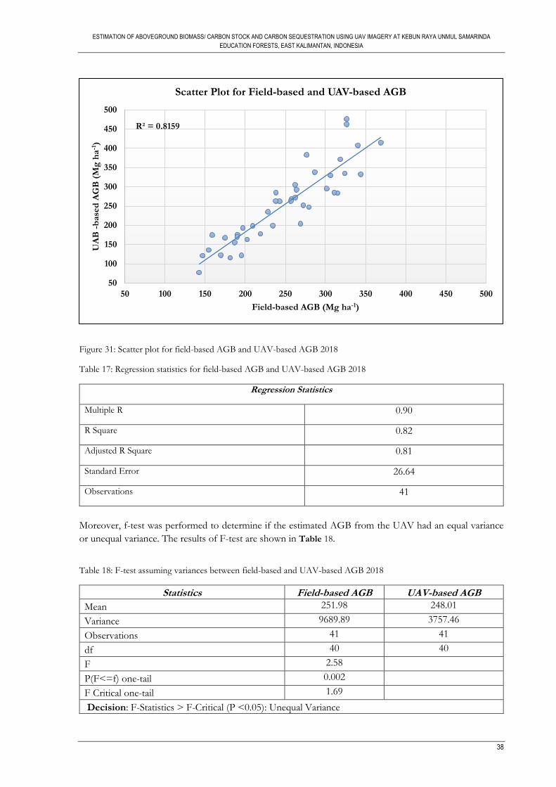
ESTIMATION OF ABOVEGROUND BIOMASS/ CARBON STOCK AND CARBON SEQUESTRATION USING UAV IMAGERY AT KEBUN RAYA UNMUL SAMARINDA
EDUCATION FORESTS, EAST KALIMANTAN, INDONESIA
38
Figure 31: Scatter plot for field-based AGB and UAV-based AGB 2018
Table 17: Regression statistics for field-based AGB and UAV-based AGB 2018
Regression Statistics
Multiple R 0.90
R Square 0.82
Adjusted R Square 0.81
Standard Error 26.64
Observations 41
Moreover, f-test was performed to determine if the estimated AGB from the UAV had an equal variance
or unequal variance. The results of F-test are shown in Table 18.
Table 18: F-test assuming variances between field-based and UAV-based AGB 2018
Statistics Field-based AGB UAV-based AGB
Mean 251.98 248.01
Variance 9689.89 3757.46
Observations 41 41
df 40 40
F 2.58
P(F<=f) one-tail 0.002
F Critical one-tail 1.69
Decision: F-Statistics > F-Critical (P <0.05): Unequal Variance
R² = 0.8159
50
100
150
200
250
300
350
400
450
500
50 100 150 200 250 300 350 400 450 500
UA
B -
base
d A
GB
(M
g h
a-1)
Field-based AGB (Mg ha-1)
Scatter Plot for Field-based and UAV-based AGB
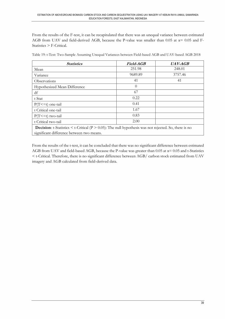
ESTIMATION OF ABOVEGROUND BIOMASS/ CARBON STOCK AND CARBON SEQUESTRATION USING UAV IMAGERY AT KEBUN RAYA UNMUL SAMARINDA
EDUCATION FORESTS, EAST KALIMANTAN, INDONESIA
39
From the results of the F-test, it can be recapitulated that there was an unequal variance between estimated
AGB from UAV and field-derived AGB, because the P-value was smaller than 0.05 at α= 0.05 and F-
Statistics > F-Critical. Table 19: t-Test: Two-Sample Assuming Unequal Variances between Field-based AGB and UAV-based AGB 2018
Statistics Field-AGB UAV-AGB
Mean 251.98 248.01
Variance 9689.89 3757.46
Observations 41 41
Hypothesized Mean Difference 0
df 67
t Stat 0.22
P(T<=t) one-tail 0.41
t Critical one-tail 1.67
P(T<=t) two-tail 0.83
t Critical two-tail 2.00
Decision: t-Statistics < t-Critical (P > 0.05): The null hypothesis was not rejected. So, there is no
significant difference between two means.
From the results of the t-test, it can be concluded that there was no significant difference between estimated
AGB from UAV and field-based AGB, because the P-value was greater than 0.05 at α= 0.05 and t-Statistics
< t-Critical. Therefore, there is no significant difference between AGB/ carbon stock estimated from UAV
imagery and AGB calculated from field-derived data.
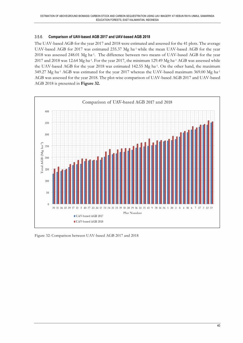
ESTIMATION OF ABOVEGROUND BIOMASS/ CARBON STOCK AND CARBON SEQUESTRATION USING UAV IMAGERY AT KEBUN RAYA UNMUL SAMARINDA
EDUCATION FORESTS, EAST KALIMANTAN, INDONESIA
40
Comparison of UAV-based AGB 2017 and UAV-based AGB 2018
The UAV-based AGB for the year 2017 and 2018 were estimated and assessed for the 41 plots. The average
UAV-based AGB for 2017 was estimated 235.37 Mg ha-1 while the mean UAV-based AGB for the year
2018 was assessed 248.01 Mg ha-1. The difference between two means of UAV-based AGB for the year
2017 and 2018 was 12.64 Mg ha-1. For the year 2017, the minimum 129.49 Mg ha-1 AGB was assessed while
the UAV-based AGB for the year 2018 was estimated 142.55 Mg ha-1. On the other hand, the maximum
349.27 Mg ha-1 AGB was estimated for the year 2017 whereas the UAV-based maximum 369.00 Mg ha-1
AGB was assessed for the year 2018. The plot-wise comparison of UAV-based AGB 2017 and UAV-based
AGB 2018 is presented in Figure 32.
Figure 32: Comparison between UAV-based AGB 2017 and 2018
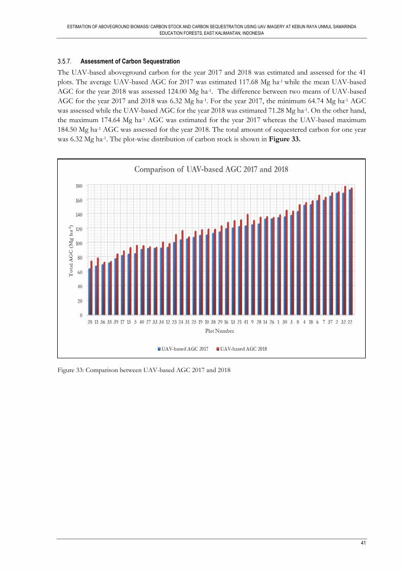
ESTIMATION OF ABOVEGROUND BIOMASS/ CARBON STOCK AND CARBON SEQUESTRATION USING UAV IMAGERY AT KEBUN RAYA UNMUL SAMARINDA
EDUCATION FORESTS, EAST KALIMANTAN, INDONESIA
41
Assessment of Carbon Sequestration
The UAV-based aboveground carbon for the year 2017 and 2018 was estimated and assessed for the 41
plots. The average UAV-based AGC for 2017 was estimated 117.68 Mg ha-1 while the mean UAV-based
AGC for the year 2018 was assessed 124.00 Mg ha-1. The difference between two means of UAV-based
AGC for the year 2017 and 2018 was 6.32 Mg ha-1. For the year 2017, the minimum 64.74 Mg ha-1 AGC
was assessed while the UAV-based AGC for the year 2018 was estimated 71.28 Mg ha-1. On the other hand,
the maximum 174.64 Mg ha-1 AGC was estimated for the year 2017 whereas the UAV-based maximum
184.50 Mg ha-1 AGC was assessed for the year 2018. The total amount of sequestered carbon for one year
was 6.32 Mg ha-1. The plot-wise distribution of carbon stock is shown in Figure 33.
Figure 33: Comparison between UAV-based AGC 2017 and 2018
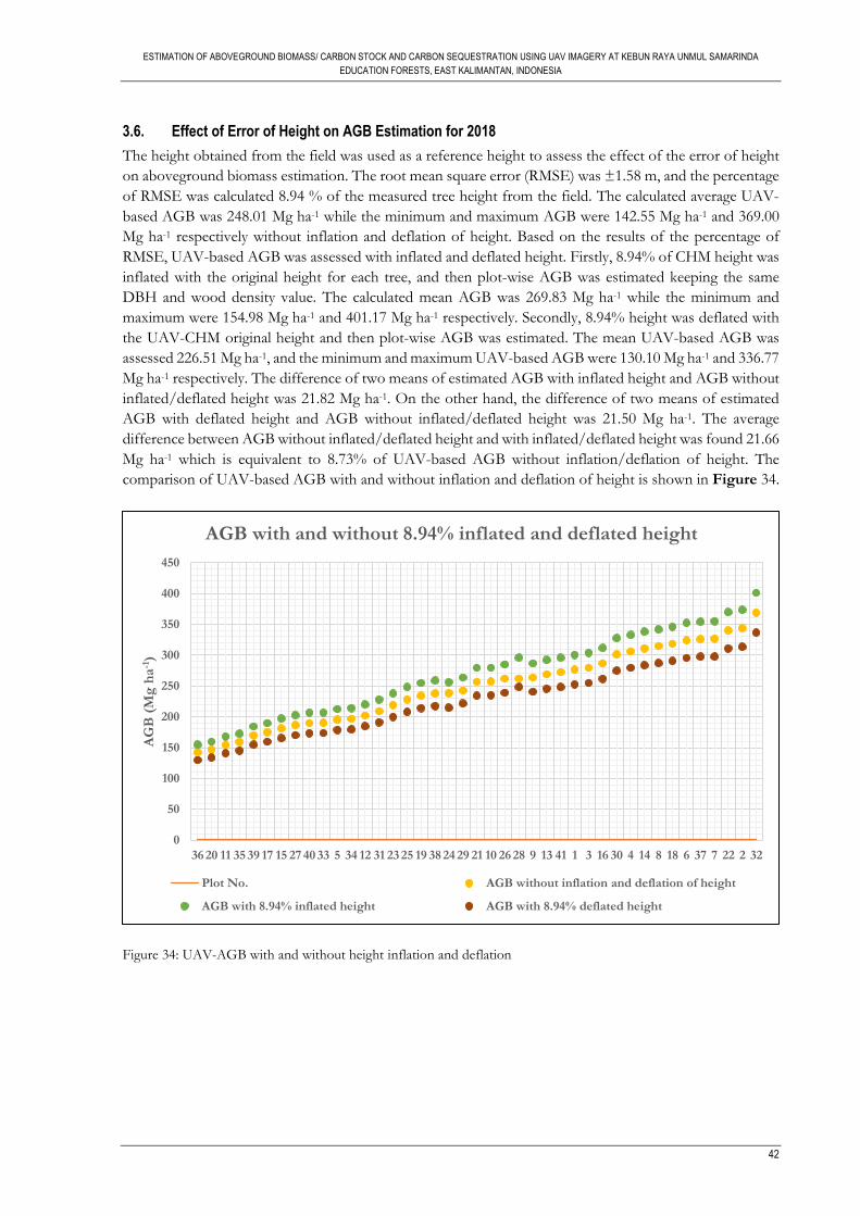
ESTIMATION OF ABOVEGROUND BIOMASS/ CARBON STOCK AND CARBON SEQUESTRATION USING UAV IMAGERY AT KEBUN RAYA UNMUL SAMARINDA
EDUCATION FORESTS, EAST KALIMANTAN, INDONESIA
42
3.6. Effect of Error of Height on AGB Estimation for 2018
The height obtained from the field was used as a reference height to assess the effect of the error of height
on aboveground biomass estimation. The root mean square error (RMSE) was ±1.58 m, and the percentage
of RMSE was calculated 8.94 % of the measured tree height from the field. The calculated average UAV-
based AGB was 248.01 Mg ha-1 while the minimum and maximum AGB were 142.55 Mg ha-1 and 369.00
Mg ha-1 respectively without inflation and deflation of height. Based on the results of the percentage of
RMSE, UAV-based AGB was assessed with inflated and deflated height. Firstly, 8.94% of CHM height was
inflated with the original height for each tree, and then plot-wise AGB was estimated keeping the same
DBH and wood density value. The calculated mean AGB was 269.83 Mg ha-1 while the minimum and
maximum were 154.98 Mg ha-1 and 401.17 Mg ha-1 respectively. Secondly, 8.94% height was deflated with
the UAV-CHM original height and then plot-wise AGB was estimated. The mean UAV-based AGB was
assessed 226.51 Mg ha-1, and the minimum and maximum UAV-based AGB were 130.10 Mg ha-1 and 336.77
Mg ha-1 respectively. The difference of two means of estimated AGB with inflated height and AGB without
inflated/deflated height was 21.82 Mg ha-1. On the other hand, the difference of two means of estimated
AGB with deflated height and AGB without inflated/deflated height was 21.50 Mg ha-1. The average
difference between AGB without inflated/deflated height and with inflated/deflated height was found 21.66
Mg ha-1 which is equivalent to 8.73% of UAV-based AGB without inflation/deflation of height. The
comparison of UAV-based AGB with and without inflation and deflation of height is shown in Figure 34.
Figure 34: UAV-AGB with and without height inflation and deflation
0
50
100
150
200
250
300
350
400
450
36 20 11 35 39 17 15 27 40 33 5 34 12 31 23 25 19 38 24 29 21 10 26 28 9 13 41 1 3 16 30 4 14 8 18 6 37 7 22 2 32
AG
B (
Mg
ha
-1)
AGB with and without 8.94% inflated and deflated height
Plot No. AGB without inflation and deflation of height
AGB with 8.94% inflated height AGB with 8.94% deflated height
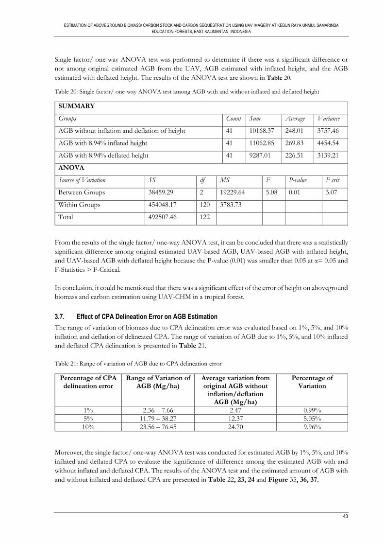
ESTIMATION OF ABOVEGROUND BIOMASS/ CARBON STOCK AND CARBON SEQUESTRATION USING UAV IMAGERY AT KEBUN RAYA UNMUL SAMARINDA
EDUCATION FORESTS, EAST KALIMANTAN, INDONESIA
43
Single factor/ one-way ANOVA test was performed to determine if there was a significant difference or
not among original estimated AGB from the UAV, AGB estimated with inflated height, and the AGB
estimated with deflated height. The results of the ANOVA test are shown in Table 20.
Table 20: Single factor/ one-way ANOVA test among AGB with and without inflated and deflated height
SUMMARY
Groups Count Sum Average Variance
AGB without inflation and deflation of height 41 10168.37 248.01 3757.46
AGB with 8.94% inflated height 41 11062.85 269.83 4454.54
AGB with 8.94% deflated height 41 9287.01 226.51 3139.21
ANOVA
Source of Variation SS df MS F P-value F crit
Between Groups 38459.29 2 19229.64 5.08 0.01 3.07
Within Groups 454048.17 120 3783.73
Total 492507.46 122
From the results of the single factor/ one-way ANOVA test, it can be concluded that there was a statistically
significant difference among original estimated UAV-based AGB, UAV-based AGB with inflated height,
and UAV-based AGB with deflated height because the P-value (0.01) was smaller than 0.05 at α= 0.05 and
F-Statistics > F-Critical.
In conclusion, it could be mentioned that there was a significant effect of the error of height on aboveground
biomass and carbon estimation using UAV-CHM in a tropical forest.
3.7. Effect of CPA Delineation Error on AGB Estimation
The range of variation of biomass due to CPA delineation error was evaluated based on 1%, 5%, and 10%
inflation and deflation of delineated CPA. The range of variation of AGB due to 1%, 5%, and 10% inflated
and deflated CPA delineation is presented in Table 21.
Table 21: Range of variation of AGB due to CPA delineation error
Percentage of CPA delineation error
Range of Variation of AGB (Mg/ha)
Average variation from original AGB without
inflation/deflation AGB (Mg/ha)
Percentage of Variation
1% 2.36 – 7.66 2.47 0.99%
5% 11.79 – 38.27 12.37 5.05%
10% 23.56 – 76.45 24.70 9.96%
Moreover, the single factor/ one-way ANOVA test was conducted for estimated AGB by 1%, 5%, and 10%
inflated and deflated CPA to evaluate the significance of difference among the estimated AGB with and
without inflated and deflated CPA. The results of the ANOVA test and the estimated amount of AGB with
and without inflated and deflated CPA are presented in Table 22, 23, 24 and Figure 35, 36, 37.
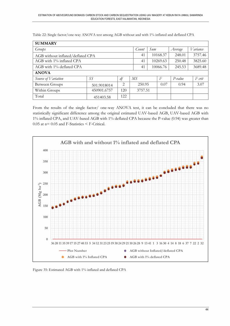
ESTIMATION OF ABOVEGROUND BIOMASS/ CARBON STOCK AND CARBON SEQUESTRATION USING UAV IMAGERY AT KEBUN RAYA UNMUL SAMARINDA
EDUCATION FORESTS, EAST KALIMANTAN, INDONESIA
44
Table 22: Single factor/one-way ANOVA test among AGB without and with 1% inflated and deflated CPA
SUMMARY
Groups Count Sum Average Variance
AGB without inflated/deflated CPA 41 10168.37 248.01 3757.46
AGB with 1% inflated CPA 41 10269.63 250.48 3825.60
AGB with 1% deflated CPA 41 10066.76 245.53 3689.48
ANOVA
Source of Variation SS df MS F P-value F crit
Between Groups 501.9018014 2 250.95 0.07 0.94 3.07
Within Groups 450901.6757 120 3757.51
Total 451403.58 122
From the results of the single factor/ one-way ANOVA test, it can be concluded that there was no
statistically significant difference among the original estimated UAV-based AGB, UAV-based AGB with
1% inflated CPA, and UAV-based AGB with 1% deflated CPA because the P-value (0.94) was greater than
0.05 at α= 0.05 and F-Statistics < F-Critical.
Figure 35: Estimated AGB with 1% inflated and deflated CPA
0
50
100
150
200
250
300
350
400
36 20 11 35 39 17 15 27 40 33 5 34 12 31 23 25 19 38 24 29 21 10 26 28 9 13 41 1 3 16 30 4 14 8 18 6 37 7 22 2 32
AG
B (
Mg
ha
-1)
AGB with and without 1% inflated and deflated CPA
Plot Number AGB without Inflated/deflated CPA
AGB with 1% Inflated CPA AGB with 1% deflated CPA
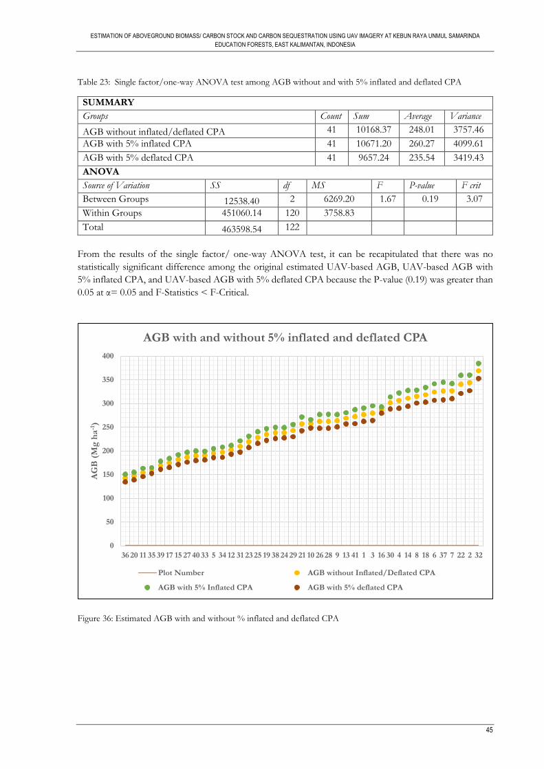
ESTIMATION OF ABOVEGROUND BIOMASS/ CARBON STOCK AND CARBON SEQUESTRATION USING UAV IMAGERY AT KEBUN RAYA UNMUL SAMARINDA
EDUCATION FORESTS, EAST KALIMANTAN, INDONESIA
45
Table 23: Single factor/one-way ANOVA test among AGB without and with 5% inflated and deflated CPA
SUMMARY
Groups Count Sum Average Variance
AGB without inflated/deflated CPA 41 10168.37 248.01 3757.46
AGB with 5% inflated CPA 41 10671.20 260.27 4099.61
AGB with 5% deflated CPA 41 9657.24 235.54 3419.43
ANOVA
Source of Variation SS df MS F P-value F crit
Between Groups 12538.40 2 6269.20 1.67 0.19 3.07
Within Groups 451060.14 120 3758.83
Total 463598.54 122
From the results of the single factor/ one-way ANOVA test, it can be recapitulated that there was no
statistically significant difference among the original estimated UAV-based AGB, UAV-based AGB with
5% inflated CPA, and UAV-based AGB with 5% deflated CPA because the P-value (0.19) was greater than
0.05 at α= 0.05 and F-Statistics < F-Critical.
Figure 36: Estimated AGB with and without % inflated and deflated CPA
0
50
100
150
200
250
300
350
400
36 20 11 35 39 17 15 27 40 33 5 34 12 31 23 25 19 38 24 29 21 10 26 28 9 13 41 1 3 16 30 4 14 8 18 6 37 7 22 2 32
AG
B (
Mg
ha
-1)
AGB with and without 5% inflated and deflated CPA
Plot Number AGB without Inflated/Deflated CPA
AGB with 5% Inflated CPA AGB with 5% deflated CPA
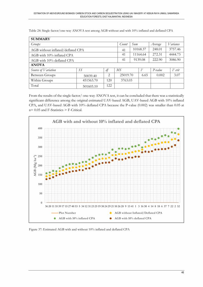
ESTIMATION OF ABOVEGROUND BIOMASS/ CARBON STOCK AND CARBON SEQUESTRATION USING UAV IMAGERY AT KEBUN RAYA UNMUL SAMARINDA
EDUCATION FORESTS, EAST KALIMANTAN, INDONESIA
46
Table 24: Single factor/one-way ANOVA test among AGB without and with 10% inflated and deflated CPA
SUMMARY
Groups Count Sum Average Variance
AGB without inflated/deflated CPA 41 10168.37 248.01 3757.46
AGB with 10% inflated CPA 41 11164.64 272.31 4444.73
AGB with 10% deflated CPA 41 9139.08 222.90 3086.90
ANOVA
Source of Variation SS df MS F P-value F crit
Between Groups 50039.40 2 25019.70 6.65 0.002 3.07
Within Groups 451563.70 120 3763.03
Total 501603.10 122
From the results of the single factor/ one-way ANOVA test, it can be concluded that there was a statistically
significant difference among the original estimated UAV-based AGB, UAV-based AGB with 10% inflated
CPA, and UAV-based AGB with 10% deflated CPA because the P-value (0.002) was smaller than 0.05 at
α= 0.05 and F-Statistics > F-Critical.
Figure 37: Estimated AGB with and without 10% inflated and deflated CPA
0
50
100
150
200
250
300
350
400
36 20 11 35 39 17 15 27 40 33 5 34 12 31 23 25 19 38 24 29 21 10 26 28 9 13 41 1 3 16 30 4 14 8 18 6 37 7 22 2 32
AG
B (
Mg
ha
-1)
AGB with and without 10% inflated and deflated CPA
Plot Number AGB without Inflated/Deflated CPA
AGB with 10% inflated CPA AGB with 10% deflated CPA
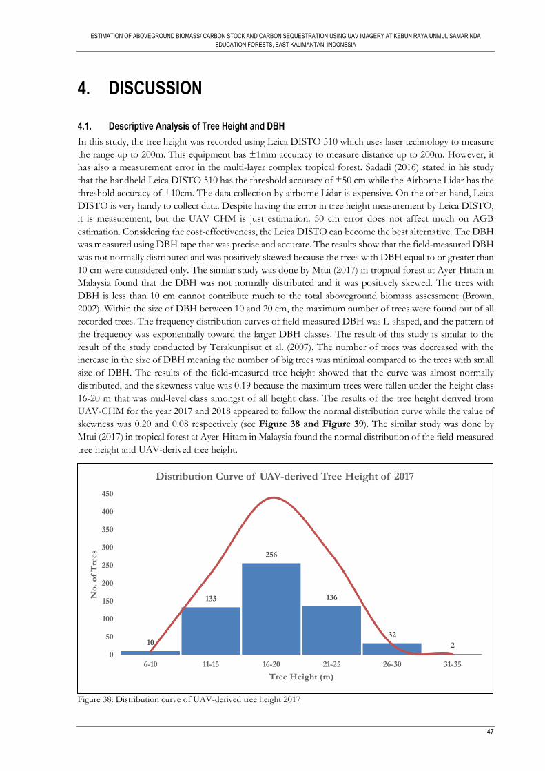
ESTIMATION OF ABOVEGROUND BIOMASS/ CARBON STOCK AND CARBON SEQUESTRATION USING UAV IMAGERY AT KEBUN RAYA UNMUL SAMARINDA
EDUCATION FORESTS, EAST KALIMANTAN, INDONESIA
47
4. DISCUSSION
4.1. Descriptive Analysis of Tree Height and DBH
In this study, the tree height was recorded using Leica DISTO 510 which uses laser technology to measure
the range up to 200m. This equipment has ±1mm accuracy to measure distance up to 200m. However, it
has also a measurement error in the multi-layer complex tropical forest. Sadadi (2016) stated in his study
that the handheld Leica DISTO 510 has the threshold accuracy of ±50 cm while the Airborne Lidar has the
threshold accuracy of ±10cm. The data collection by airborne Lidar is expensive. On the other hand, Leica
DISTO is very handy to collect data. Despite having the error in tree height measurement by Leica DISTO,
it is measurement, but the UAV CHM is just estimation. 50 cm error does not affect much on AGB
estimation. Considering the cost-effectiveness, the Leica DISTO can become the best alternative. The DBH
was measured using DBH tape that was precise and accurate. The results show that the field-measured DBH
was not normally distributed and was positively skewed because the trees with DBH equal to or greater than
10 cm were considered only. The similar study was done by Mtui (2017) in tropical forest at Ayer-Hitam in
Malaysia found that the DBH was not normally distributed and it was positively skewed. The trees with
DBH is less than 10 cm cannot contribute much to the total aboveground biomass assessment (Brown,
2002). Within the size of DBH between 10 and 20 cm, the maximum number of trees were found out of all
recorded trees. The frequency distribution curves of field-measured DBH was L-shaped, and the pattern of
the frequency was exponentially toward the larger DBH classes. The result of this study is similar to the
result of the study conducted by Terakunpisut et al. (2007). The number of trees was decreased with the
increase in the size of DBH meaning the number of big trees was minimal compared to the trees with small
size of DBH. The results of the field-measured tree height showed that the curve was almost normally
distributed, and the skewness value was 0.19 because the maximum trees were fallen under the height class
16-20 m that was mid-level class amongst of all height class. The results of the tree height derived from
UAV-CHM for the year 2017 and 2018 appeared to follow the normal distribution curve while the value of
skewness was 0.20 and 0.08 respectively (see Figure 38 and Figure 39). The similar study was done by
Mtui (2017) in tropical forest at Ayer-Hitam in Malaysia found the normal distribution of the field-measured
tree height and UAV-derived tree height.
Figure 38: Distribution curve of UAV-derived tree height 2017
10
133
256
136
32
20
50
100
150
200
250
300
350
400
450
6-10 11-15 16-20 21-25 26-30 31-35
No
. o
f T
rees
Tree Height (m)
Distribution Curve of UAV-derived Tree Height of 2017
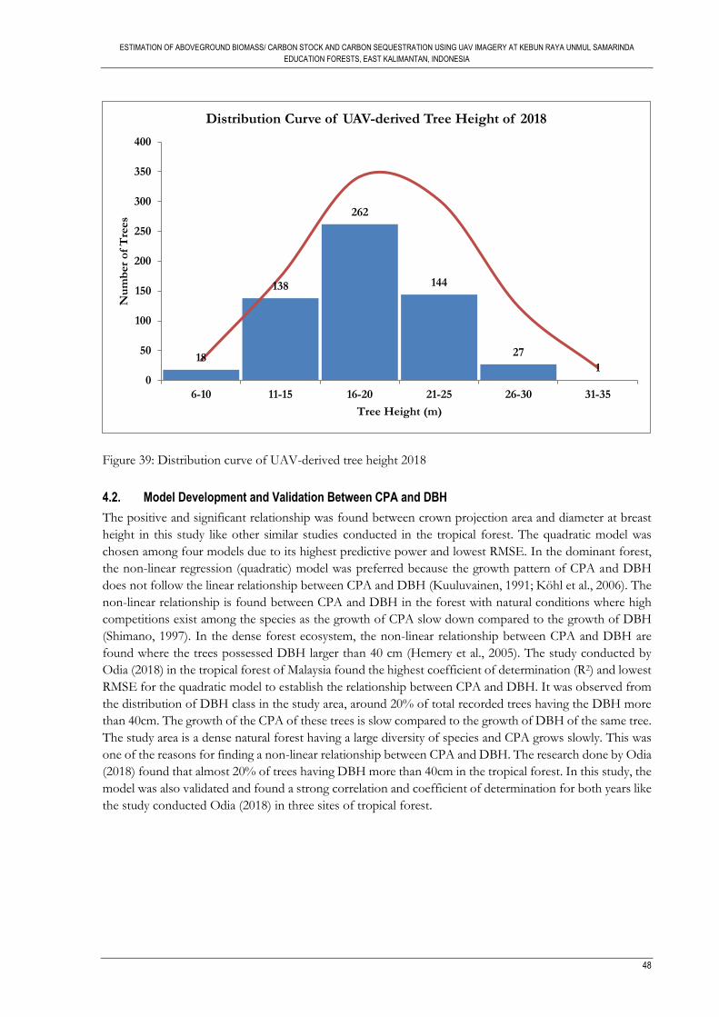
ESTIMATION OF ABOVEGROUND BIOMASS/ CARBON STOCK AND CARBON SEQUESTRATION USING UAV IMAGERY AT KEBUN RAYA UNMUL SAMARINDA
EDUCATION FORESTS, EAST KALIMANTAN, INDONESIA
48
Figure 39: Distribution curve of UAV-derived tree height 2018
4.2. Model Development and Validation Between CPA and DBH
The positive and significant relationship was found between crown projection area and diameter at breast
height in this study like other similar studies conducted in the tropical forest. The quadratic model was
chosen among four models due to its highest predictive power and lowest RMSE. In the dominant forest,
the non-linear regression (quadratic) model was preferred because the growth pattern of CPA and DBH
does not follow the linear relationship between CPA and DBH (Kuuluvainen, 1991; Köhl et al., 2006). The
non-linear relationship is found between CPA and DBH in the forest with natural conditions where high
competitions exist among the species as the growth of CPA slow down compared to the growth of DBH
(Shimano, 1997). In the dense forest ecosystem, the non-linear relationship between CPA and DBH are
found where the trees possessed DBH larger than 40 cm (Hemery et al., 2005). The study conducted by
Odia (2018) in the tropical forest of Malaysia found the highest coefficient of determination (R2) and lowest
RMSE for the quadratic model to establish the relationship between CPA and DBH. It was observed from
the distribution of DBH class in the study area, around 20% of total recorded trees having the DBH more
than 40cm. The growth of the CPA of these trees is slow compared to the growth of DBH of the same tree.
The study area is a dense natural forest having a large diversity of species and CPA grows slowly. This was
one of the reasons for finding a non-linear relationship between CPA and DBH. The research done by Odia
(2018) found that almost 20% of trees having DBH more than 40cm in the tropical forest. In this study, the
model was also validated and found a strong correlation and coefficient of determination for both years like
the study conducted Odia (2018) in three sites of tropical forest.
18
138
262
144
27
10
50
100
150
200
250
300
350
400
6-10 11-15 16-20 21-25 26-30 31-35
Nu
mb
er
of
Tre
es
Tree Height (m)
Distribution Curve of UAV-derived Tree Height of 2018
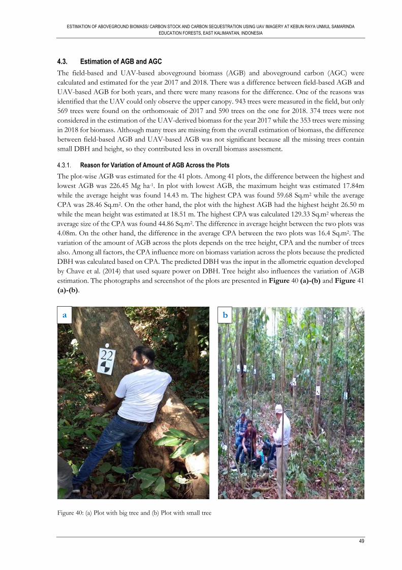
ESTIMATION OF ABOVEGROUND BIOMASS/ CARBON STOCK AND CARBON SEQUESTRATION USING UAV IMAGERY AT KEBUN RAYA UNMUL SAMARINDA
EDUCATION FORESTS, EAST KALIMANTAN, INDONESIA
49
4.3. Estimation of AGB and AGC
The field-based and UAV-based aboveground biomass (AGB) and aboveground carbon (AGC) were
calculated and estimated for the year 2017 and 2018. There was a difference between field-based AGB and
UAV-based AGB for both years, and there were many reasons for the difference. One of the reasons was
identified that the UAV could only observe the upper canopy. 943 trees were measured in the field, but only
569 trees were found on the orthomosaic of 2017 and 590 trees on the one for 2018. 374 trees were not
considered in the estimation of the UAV-derived biomass for the year 2017 while the 353 trees were missing
in 2018 for biomass. Although many trees are missing from the overall estimation of biomass, the difference
between field-based AGB and UAV-based AGB was not significant because all the missing trees contain
small DBH and height, so they contributed less in overall biomass assessment.
Reason for Variation of Amount of AGB Across the Plots
The plot-wise AGB was estimated for the 41 plots. Among 41 plots, the difference between the highest and
lowest AGB was 226.45 Mg ha-1. In plot with lowest AGB, the maximum height was estimated 17.84m
while the average height was found 14.43 m. The highest CPA was found 59.68 Sq.m2 while the average
CPA was 28.46 Sq.m2. On the other hand, the plot with the highest AGB had the highest height 26.50 m
while the mean height was estimated at 18.51 m. The highest CPA was calculated 129.33 Sq.m2 whereas the
average size of the CPA was found 44.86 Sq.m2. The difference in average height between the two plots was
4.08m. On the other hand, the difference in the average CPA between the two plots was 16.4 Sq.m2. The
variation of the amount of AGB across the plots depends on the tree height, CPA and the number of trees
also. Among all factors, the CPA influence more on biomass variation across the plots because the predicted
DBH was calculated based on CPA. The predicted DBH was the input in the allometric equation developed
by Chave et al. (2014) that used square power on DBH. Tree height also influences the variation of AGB
estimation. The photographs and screenshot of the plots are presented in Figure 40 (a)-(b) and Figure 41
(a)-(b).
Figure 40: (a) Plot with big tree and (b) Plot with small tree
b a
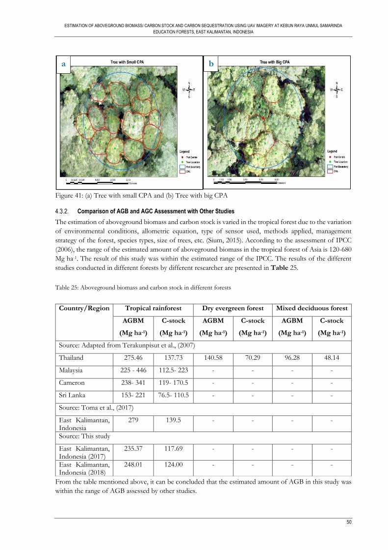
ESTIMATION OF ABOVEGROUND BIOMASS/ CARBON STOCK AND CARBON SEQUESTRATION USING UAV IMAGERY AT KEBUN RAYA UNMUL SAMARINDA
EDUCATION FORESTS, EAST KALIMANTAN, INDONESIA
50
Figure 41: (a) Tree with small CPA and (b) Tree with big CPA
Comparison of AGB and AGC Assessment with Other Studies
The estimation of aboveground biomass and carbon stock is varied in the tropical forest due to the variation
of environmental conditions, allometric equation, type of sensor used, methods applied, management
strategy of the forest, species types, size of trees, etc. (Sium, 2015). According to the assessment of IPCC
(2006), the range of the estimated amount of aboveground biomass in the tropical forest of Asia is 120-680
Mg ha-1. The result of this study was within the estimated range of the IPCC. The results of the different
studies conducted in different forests by different researcher are presented in Table 25.
Table 25: Aboveground biomass and carbon stock in different forests
From the table mentioned above, it can be concluded that the estimated amount of AGB in this study was
within the range of AGB assessed by other studies.
Country/Region Tropical rainforest Dry evergreen forest Mixed deciduous forest
AGBM
(Mg ha-1)
C-stock
(Mg ha-1)
AGBM
(Mg ha-1)
C-stock
(Mg ha-1)
AGBM
(Mg ha-1)
C-stock
(Mg ha-1)
Source: Adapted from Terakunpisut et al., (2007)
Thailand 275.46 137.73 140.58 70.29 96.28 48.14
Malaysia 225 - 446 112.5- 223 - - - -
Cameron 238- 341 119- 170.5 - - - -
Sri Lanka 153- 221 76.5- 110.5 - - - -
Source: Toma et al., (2017)
East Kalimantan, Indonesia
279 139.5 - - - -
Source: This study
East Kalimantan, Indonesia (2017)
235.37 117.69 - - - -
East Kalimantan, Indonesia (2018)
248.01 124.00 - - - -
a b
ESTIMATION OF ABOVEGROUND BIOMASS/ CARBON STOCK AND CARBON SEQUESTRATION USING UAV IMAGERY AT KEBUN RAYA UNMUL SAMARINDA
EDUCATION FORESTS, EAST KALIMANTAN, INDONESIA
51
4.4. Assessment of Carbon Sequestration
The UAV-based aboveground carbon for the year 2017 and 2018 was estimated and assessed for the 41
plots. The total amount of sequestered carbon for one year was 6.32 Mg ha-1. Sedjo (1989) applied a universal
average rate of 6.24 Mg C/ha/yr in his study which was very much close to the result of this study. A study
conducted by Diana et al. (2002) found the amount of sequestered carbon for the species Acacia mangium,
Eucalyptus pelitta, and Gmelina arborea were 5.9-9.9, 7.1-7.2, 8.3-12.3 Mg ha-1y-1. The result of this study was
similar to and within the range of AGB of these three species. A study conducted on the tropical forest by
Brown, (1992) produced a table mentioning the amount of sequestering carbon assessed by the different
researcher in different types of tropical forest (see Table 26).
Table 26: Carbon sequestration in different tropical forests
Forest Type Dry Matter Carbon Studied By Source
Mg/ha/year Mg/ha/year
Tropical rainforest 7.75- 10.19 3.88- 5.10 Bolin et al. (1986) (various sites)
Source: Adapted from Brown, (1992)
Seasonal tropical forest 5.50- 7.20 2.75- 3.60
Rainforest (Manaus) 15.00 7.50 Cannell (1982)
Rainforest (Ivory Coast) 12.73- 24.60 6.36- 12.30
Amazonian rainforest (mean)
12.66 6.33 Jordan (1989)
Slash and burn (after 3 years)
5.26 2.62
From the table, it can be mentioned that the estimated amount of sequestered carbon in this study was very
much close to the estimated amount of sequestered carbon in Amazonian rainforest and rainforest of Ivory
Coast. The assessed sequestered carbon in this study was higher than the range of sequestered carbon
estimated for tropical rainforest and seasonal tropical rainforest by Bolin et al. (1986) in various sites. This
variation occurred due to different forest structure, different tree species and the size of the trees, etc.
4.5. Effect of Tree Parameters Error on AGB Estimation
The tree parameters extracted from the UAV images influence the biomass estimation. The inflated and
deflated tree height and CPA were used to evaluate the variation of biomass. The difference of UAV-based
AGB with and without inflated/deflated height was found 21.66 Mg ha-1 which was equivalent to 8.73% of
original estimated UAV-based AGB without inflation and deflation of height. The single factor/ one-way
ANOVA test revealed that there was a statistically significant difference between estimated UAV-based
AGB with 8.94% inflation and deflation of height and UAV-based AGB without inflation/deflation of
height. The study conducted by Okojie (2017) found that the estimation of biomass was significantly
influenced by the variation of height. The study conducted by Hunter et al. (2013) also found that the
influence of height imprecision on biomass assessment is approximately 6%. In this study, the difference of
UAV-based assessed carbon with and without height inflation and deflation was bigger than the total
amount of sequestered carbon for one year. In this study, the field-based tree height measured by Leica
DISTO 510 was used as a reference height that has ±50 cm inaccuracy. This level of inaccuracy has
uncertainty in assessing AGB. This level of inaccuracy was not considered in this study because there was
no other best alternative that was cost-effective to collect tree height. Despite the certain level of inaccuracy
in Leica DISTO 510, this height is measurement, but the CHM is an estimation. The accuracy of the CHM
depends on the density of the point clouds.
ESTIMATION OF ABOVEGROUND BIOMASS/ CARBON STOCK AND CARBON SEQUESTRATION USING UAV IMAGERY AT KEBUN RAYA UNMUL SAMARINDA
EDUCATION FORESTS, EAST KALIMANTAN, INDONESIA
52
The average variation of biomass due to 1% inflation and deflation of CPA was 2.47 Mg ha-1 which was
equivalent to 0.99%, and it does not influence more on biomass estimation. For 5% inflation and deflation
of CPA, the average variation of biomass was estimated 12.37 Mg ha-1. It had no statistically significant
difference from original biomass, but the amount of AGB was close to the estimated amount of sequestered
biomass for one year. On the other hand, the average variation of biomass 24.70 Mg ha-1 was estimated due
to 10% inflated and deflated CPA that showed a statistically significant difference, and it affected 9.96%
variation of biomass from the original biomass. The estimated amount of carbon caused inflation and
deflation of CPA was observed double compared to the amount of sequestered carbon for one year. The
missing tree was also responsible for the variation of AGB that was finally influenced the estimation of
carbon sequestration. Due to the missing tree, 11.05% of AGB was underestimated in the year 2018, and
9.02% of AGB was underestimated in the year 2017 compared with the field-based AGB. This has also
influence on estimating carbon sequestration.
The combined error from the tree height and the CPA delineation might be affected more on biomass
estimation. The variance of the estimated amount of carbon with height and CPA inflation/deflation and
the estimated amount of carbon without inflation and deflation might be high. This variation would be
larger while considering error for both years. The effect of tree height and CPA delineation error on biomass
estimation was bigger than the estimated amount of sequestered carbon. The estimated amount of
sequestered carbon might be the reason for error of tree height and CPA delineation. The carbon
sequestration assessment for one year might be influenced more by the error originated from the tree
parameters extraction. The total amount of sequestered carbon might be more than the estimated carbon
sequestration variation for the different type of error. The influence of different errors on carbon
sequestration estimation would be less while assessing sequestered carbon for more than one year because
the amount of sequestered carbon would be large.
4.6. Limitations
The conducted research has limitations. Some of the significant limitations are mentioned below that would
be helpful to construct recommendations for similar studies in the future.
✓ The handheld GPS named Garmin has a certain level of inaccuracy, and it was quite challenging to
identify the correct location of the respective trees and plot centers;
✓ Enough open space is needed to place the GCP marker inside the forest. In a tropical forest, it is a
very challenging task to find enough open space to put the GCP as if they are evenly distributed in
the study area;
✓ In this study, Leica DISTO 510 laser ranger was used to record the tree height. In a dense tropical
forest, it is quite challenging to measure the tree height of tall trees using Leica DISTO 510 because
of existing understory, intermingling situation, etc. It was also experienced in this study;
✓ It was not possible to select sampling plots that covered large area due to inaccessibility for mining
activities and rugged terrain with steep slopes;
ESTIMATION OF ABOVEGROUND BIOMASS/ CARBON STOCK AND CARBON SEQUESTRATION USING UAV IMAGERY AT KEBUN RAYA UNMUL SAMARINDA
EDUCATION FORESTS, EAST KALIMANTAN, INDONESIA
53
5. CONCLUSION AND RECOMMENDATIONS
5.1. Conclusion
Quantification and monitoring of carbon sequestration in the tropical rainforest is essential for
understanding the role of the tropical rainforest on the global carbon cycle. This study explored the
potentialities of using UAV to assess aboveground biomass/carbon stock and carbon sequestration of
KRUS education forest of East Kalimantan, Indonesia. The study also investigated the influence of height
and CPA delineation error on biomass and carbon sequestration estimation. To address the research
objectives and questions, the following conclusions were made based on results.
What is the estimated amount of the AGB/carbon stock for 2017 and 2018?
In 2017, the average UAV-based AGB was assessed 235.37 Mg ha-1 while the mean UAV-based AGB was
estimated at 248.01 Mg ha-1 for 2018. The difference between the two means of AGB was 12.64 Mg ha-1.
On the other hand, the average UAV-based carbon was estimated 117.69 Mg ha-1 for the year 2017 whereas,
the average UAV-based carbon was estimated 124.00 Mg ha-1 for the year 2018.
What is the estimated amount of sequestered carbon?
The amount of sequestered carbon for one year was estimated at 6.32 Mg ha-1. The total area of the KRUS
educational forest is 238 hectares. Therefore, the annual amount of sequestered carbon was estimated
1504.16 Mg.
What is the accuracy of aboveground biomass measured from UAV images?
For the year 2017, the scatter plot demonstrated the relationship between UAV-based AGB and field-based
AGB and the root mean square error (RMSE) was 42.35 Mg ha-1 which are equivalent to 18.27 % of the
field-based AGB. For the year 2018, the root mean square error (RMSE) was 50.00 Mg ha-1 which are
equivalent to 19.84 % of the field-based AGB. For both years, there was no significant difference between
estimated AGB from UAV and field-based AGB, because the P-value was greater than 0.05 at α= 0.05 and
t-Statistics < t-Critical.
What is the error of UAV-derived tree height and how does that affect the AGB estimation?
The effect of height error on biomass estimation was conducted based on the percentage of the root mean
square error (RMSE). The percentage of RMSE was calculated at 8.94% for the UAV- derived tree height
compared to the field-measured tree height. The mean difference of UAV-based AGB without
inflated/deflated height and the UAV-based AGB with inflated/deflated height was 21.66 Mg ha-1. The
8.73% biomass variation was found due to height error, and it was proved to be a significant effect on
overall plot-based biomass assessment. The resultant estimated amount of carbon stock due to height error
was greater than the amount of sequestered carbon for one year.
How much the CPA delineation error affect the AGB estimation?
The average variation of biomass due to 1% inflation and deflation of CPA was 2.47 Mg ha-1 which was
equivalent to 0.99%. The range of variation of biomass for 1% inflated and deflated CPA was 2.36 to 7.66
Mg ha-1, and it showed statistically insignificant influence on biomass estimation. For 5% inflation and
deflation of CPA, the average variation of biomass was estimated 12.37 Mg ha-1 while the range of variation
was observed 11.79- 38.27 Mg ha-1. On the other hand, the average variation of biomass 24.70 Mg ha-1 was
estimated due to 10% inflated and deflated CPA that showed a statistically significant difference, and it
affected 9.96% variation of AGB from the original biomass. The range of variation was calculated 23.56-
76.45 Mg ha-1. The estimated amount of carbon due to CPA error was double compared to the amount of
sequestered carbon for one year.
ESTIMATION OF ABOVEGROUND BIOMASS/ CARBON STOCK AND CARBON SEQUESTRATION USING UAV IMAGERY AT KEBUN RAYA UNMUL SAMARINDA
EDUCATION FORESTS, EAST KALIMANTAN, INDONESIA
54
5.2. Recommendations
✓ The handheld Garmin GPS has 5-10 m inaccuracy. It is quite challenging to identify the right tree
in the right location. Even if the center of the plot is recorded correctly, it is easy to identify the
tree location by tracing the direction of trees from the center. Therefore, Differential Global
Positioning System (DGPS) should be used to record the coordinate of the plot center to ease the
identification of individual trees within the plot because the DGPS has few centimeters error only.
✓ A large number of UAV images need more processing time. The software namely Pix4D produce
point clouds to generate DSM, DTM, and orthomosaic based on image matching technique. If
some of the images are tilted and distorted among all images, the software takes a long time to find
the tie points. The distorted DSM, DTM, and orthomosaic are produced due to the poor quality of
images. If the some of the portions of the DSM, DTM, and orthomosaic are distorted, the average
density of point clouds would be small, and the value of DSM and DTM would be higher or lower
compared to the normal range. The processing of a small number of images is better to produce
good quality DSM, DTM, and orthomosaic. Therefore, the study area should be small, and the
number of images should be reasonable to produce high-density point clouds and eventually to
generate good quality DSM, DTM, and orthomosaic.
✓ The high speed of UAV produces tilted images. Therefore, the slow or moderate speed should be
chosen as a parameter for flying UAV to get a better UAV output.
✓ Sometimes, the UAV images look good visually, but at the time of processing images, the software
does not find the tie points. It may happen for overlapping, altitude, speed, etc. of UAV flight
planning. Therefore, if the study area is located far from the origin of the researcher, the UAV
images should be processed before leaving the study area.
✓ The software namely Avanza Map should be used to identify the individual tree within the plots
during biometric data collection because it's very easy to operate
55
LIST OF REFERENCES
Affendy, H., Aminuddin, M., Razak, W., Arifin, A., Mojiol, A. R. (2009). Growth increments of indigenous species planted in secondary forest area. Research Journal of Forestry, 3(1), 23-28.doi.org/10.3923/rjf.2009.23.28
Agüera-Vega, F., Carvajal-Ramírez, F., & Martínez-Carricondo, P. (2017). Assessment of
photogrammetric mapping accuracy based on variation ground control points number using unmanned aerial vehicle. Measurement: Journal of the International Measurement Confederation, 98, 221–227. https://doi.org/10.1016/j.measurement.2016.12.002
Anderson, S. C., Kupfer, J. A., Wilson, R. R., & Cooper, R. J. (2000). Estimating forest crown area
removed by selection cutting: A linked regression-GIS approach based on stump diameters. Forest Ecology and Management, 137(1–3), 171–177. https://doi.org/10.1016/S0378-1127(99)00325-4
Asmare, M. F. (2013). Airborne LiDAR data and VHR WORLDVIEW satellite imagery to support
community based forest certification in Chitwan, Nepal (MSc Thesis). University of Twente, Faculty of Geo-Information Science and Earth Observation (ITC), Enschede,The Netherlands. Retrieved from http://www.itc.nl/library/papers_2013/msc/nrm/asmare.pdf
Basuki, T. M., van Laake, P. E., Skidmore, A. K., & Hussin, Y. A. (2009). Allometric equations for
estimating the above-ground biomass in tropical lowland Dipterocarp forests. Forest Ecology and Management, 257(8), 1684–1694. https://doi.org/10.1016/j.foreco.2009.01.027
Böttcher, H., Eisbrenner, K., Fritz, S., Kindermann, G., Kraxner, F., McCallum, I., & Obersteiner, M.
(2009). An assessment of monitoring requirements and costs of “Reduced Emissions from Deforestation and Degradation.” Carbon Balance and Management, 4, 7. https://doi.org/10.1186/1750-0680-4-7
Brown, S. (2002). Measuring carbon in forests: Current status and future challenges. Environmental Pollution,
116(3), 363–372. https://doi.org/10.1016/S0269-7491(01)00212-3 Brown, S., Sathaye, J., Cannell, M., & Kauppi, P. (1996). Management of forests for mitigation of
greenhouse gas emissions. In climate change 1995: Impacts, adaptions and mitigation of climate change: scientific-technical analyses (pp. 773–798).
Burrows, W. H., Henry, B. K., Back, P. V., Hoffmann, M. B., Tait, L. J., Anderson, E. R., … McKeon, G.
M. (2002). Growth and carbon stock change in eucalypt woodlands in northeast Australia: Ecological and greenhouse sink implications. Global Change Biology, 8(8), 769–784. https://doi.org/10.1046/j.1365-2486.2002.00515.x
Chave, J., Andalo, C., Brown, S., Cairns, M. A., Chambers, J. Q., Eamus, D., … Yamakura, T. (2005). Tree
allometry and improved estimation of carbon stocks and balance in tropical forests. Oecologia, 145(1), 87–99. https://doi.org/10.1007/s00442-005-0100-x
Chave, J., Condit, R., Aguilar, S., Hernandez, A., Lao, S., & Perez, R. (2004). Error propagation and
scaling for tropical forest biomass estimates. Philosophical Transactions of the Royal Society B: Biological Sciences, 359(1443), 409–420. https://doi.org/10.1098/rstb.2003.1425
Chave, J., Réjou-Méchain, M., Búrquez, A., Chidumayo, E., Colgan, M. S., Delitti, W. B. C., … Vieilledent,
G. (2014). Improved allometric models to estimate the aboveground biomass of tropical trees. Global Change Biology, 20(10), 3177–3190. https://doi.org/10.1111/gcb.12629
Cheng, S.-W., Dey, T. K., & Shewchuk, J. (2012). Three-dimensional delaunay triangulations. Delaunay
Mesh Generation. https://doi.org/10.1201/b12987-3
56
Clark, D. a, Brown, S., Kicklighter, D. W., Chambers, J. Q., Thomlinson, J. R., Ni, J., … Holland, E. a. (2001). Net primary production in tropical forests: an evaluation and synthesis of existing field data. Ecological Applications, 11(2), 371–384. https://doi.org/10.2307/3060895
Curtis, P. S. (2008). Estimating aboveground carbon in live and standing dead trees. In C. M. Hoover
(Ed.), Field Measurements for Forest Carbon Monitoring (pp. 39–44). Durham, NH 03824: Northern Research Station. https://doi.org/10.1007/978-1-4020-8506-2
Dandois, J. P., Olano, M., & Ellis, E. C. (2015). Optimal altitude, overlap, and weather conditions for
computer vision uav estimates of forest structure. Remote Sensing, 7(10), 13895–13920. https://doi.org/10.3390/rs71013895
Davies, S. J., & Apr, N. (2007). Tree mortality and growth in 11 sympatric macaranga species in Borneo.
Growth (Lakeland), 82(4), 920–932. https://doi.org/10.2307/2679892 Diana, R., Hadriyanto, D., Hiratsuka, M., Toma, T., & Morikawa, Y. (2002). Carbon stocks of fast growing
tree species and baselines after forest fire in east Kalimantan, Indonesia. https://doi.org/10.13140/2.1.4899.4247
Drake, J. B., Dubayah, R. O., Clark, D. B., Knox, R. G., Blair, J. B., Hofton, M. A., … Prince, S. (2002).
Estimation of tropical forest structural characteristics, using large-footprint lidar. Remote Sensing of Environment, 79(2–3), 305–319. https://doi.org/10.1016/S0034-4257(01)00281-4
Du, H., Zhou, G., Ge, H., Fan, W., Xu, X., Fan, W., & Shi, Y. (2012). Satellite-based carbon stock
estimation for bamboo forest with a non-linear partial least square regression technique. International Journal of Remote Sensing, 33(6), 1917–1933. https://doi.org/10.1080/01431161.2011.603379
Dube, T., & Mutanga, O. (2015). Evaluating the utility of the medium-spatial resolution Landsat 8
multispectral sensor in quantifying aboveground biomass in uMgeni catchment, South Africa. ISPRS Journal of Photogrammetry and Remote Sensing, 101, 36–46. https://doi.org/10.1016/j.isprsjprs.2014.11.001
Ebuy, J., Lokombe, J. P., Ponette, Q., Sonwa, D., & Picard, N. (2011). Allometric equation for predicting
aboveground biomass of three tree species. Journal of Tropical Forest Science, 23(2), 125–132. Faculty of Forestry. University of Mulawarman. (2018)(Unpublished). Forest management plan long
KPHP long-term forest management plan Unmul KRUS education forest. Fritz, A., Kattenborn, T., & Koch, B. (2013). UAV-based photogrammetric point clouds- tree stem
mapping in open stands in comparison to terrestrial laser scanner point clouds. ISPRS - International Archives of the Photogrammetry, Remote Sensing and Spatial Information Sciences, XL-1/W2(September), 141–146. https://doi.org/10.5194/isprsarchives-XL-1-W2-141-2013
Gibbs, H. K., Brown, S., Niles, J. O., & Foley, J. A. (2007). Monitoring and estimating tropical forest
carbon stocks: Making REDD a reality. Environmental Research Letters, 2(4). https://doi.org/10.1088/1748-9326/2/4/045023
Gonzalez, P., Asner, G. P., Battles, J. J., Lefsky, M. A., Waring, K. M., & Palace, M. (2010). Forest carbon
densities and uncertainties from Lidar, QuickBird, and field measurements in California. Remote Sensing of Environment, 114(7), 1561–1575. https://doi.org/10.1016/j.rse.2010.02.011
Guhardja, E., Fatawi, M., Sutisna, M., Mori, T., & Ohta, S. (2000). Rainforest ecosystems of East
Kalimantan : el Niño, drought, fire and human impacts. Ecological studies : analysis and synthesis (Vol. v. 140). Retrieved from http://ci.nii.ac.jp/ncid/BA44703883
57
Hemery, G. E., Savill, P. S., & Pryor, S. N. (2005). Applications of the crown diameter-stem diameter relationship for different species of broadleaved trees. Forest Ecology and Management, 215(1–3), 285–294. https://doi.org/10.1016/j.foreco.2005.05.016
Ho Tong Minh, D., Le Toan, T., Rocca, F., Tebaldini, S., D’Alessandro, M. M., & Villard, L. (2014).
Relating P-band synthetic aperture radar tomography to tropical forest biomass. IEEE Transactions on Geoscience and Remote Sensing, 52(2), 967–979. https://doi.org/10.1109/TGRS.2013.2246170
Holdaway, R. J., McNeill, S. J., Mason, N. W. H., & Carswell, F. E. (2014). Propagating uncertainty in
plot-based estimates of forest carbon stock and carbon stock change. Ecosystems, 17(4), 627–640. https://doi.org/10.1007/s10021-014-9749-5
Houghton, R. A., & Hackler, J. L. (2000). Changes in terrestrial carbon storage in the United States. 1: The
roles of agriculture and forestry. Global Ecology and Biogeography, 9(2), 125–144. https://doi.org/10.1046/j.1365-2699.2000.00166.x
Hunter, M. O., Keller, M., Victoria, D., & Morton, D. C. (2013). Tree height and tropical forest biomass
estimation. Biogeosciences, 10(12), 8385–8399. https://doi.org/10.5194/bg-10-8385-2013 IPCC. (2003). Good practice guidance for land use, land use change and forestry. Institute for Global Environmental
Strategies. https://doi.org/citeulike-article-id:1260638 IPCC. (2006). Volume 4: Agriculture, forestry and other land use (AFOLU). Draft 2006 IPCC guidelines for
national greenhouse gas inventories, 4, 673. Retrieved from https://www.ipcc.ch/meetings/session25/doc4a4b/vol4.pdf
Terakunpisut, J., Gajaseni, N., Ruankawe, N. (2007). Carbon sequestration potential in aboveground
biomass of Thong Pha Phum national forest, Thailand. Applied Ecology and Environmental Research, 5(P 2728), 93–102.
Kachamba, D. J., Ørka, H. O., Gobakken, T., Eid, T., & Mwase, W. (2016). Biomass estimation using 3D
data from unmanned aerial vehicle imagery in a tropical woodland. Remote Sensing, 8(11). https://doi.org/10.3390/rs8110968
Ketterings, Q. M., Coe, R., Van Noordwijk, M., Ambagau, Y., & Palm, C. A. (2001). Reducing uncertain in
the use of allometric biomass equation for predciting above-ground tree biomass in mixed secondary forests. Forest Ecology and Management, 146, 199–209. https://doi.org/
Koh, L. P., & Wich, S. A. (2012). Dawn of drone ecology: Low-cost autonomous aerial vehicles for
conservation. Tropical Conservation Science, 5(2), 121–132. https://doi.org/10.1177/194008291200500202
Köhl, M., Magnussen, S., & Marchetti, M. (2006). Sampling Methods, Remote Sensing and GIS
Multiresource Forest Inventory. Tropical Forest Ecology. https://doi.org/10.1007/978-3-540-32572-7 Kuuluvainen, T. (1991). Relationships between crown projected area and components of above-ground
biomass in Norway spruce trees in even-aged stands: Empirical results and their interpretation. Forest Ecology and Management, 40(3–4), 243–260. https://doi.org/10.1016/0378-1127(91)90043-U
Lo, E. (2005). Gaussian error propagation applied to ecological data: Post-ice-storm- downed woody
biomass. Ecological Monographs, 75(4), 451–466. https://doi.org/10.1890/05-0030 Lu, D., Mausel, P., Brondízio, E., & Moran, E. (2004). Relationships between forest stand parameters and
Landsat TM spectral responses in the Brazilian Amazon Basin. Forest Ecology and Management, 198(1–3), 149–167. https://doi.org/10.1016/j.foreco.2004.03.048
58
Magar, A. T. (2014). Estimation and mapping of forest biomass and carbon using point-clouds derived from airborne LiDAR and from 3D photogrammetric matching of aerial images, 79. Retrieved from http://www.itc.nl/library/papers_2014/msc/gem/thapamagar.pdf
Micheletti, N., Chandler, J. H., & Lane, S. N. (2015). Structure from motion (SfM) photogrammetry. British Society for Geomorphology Geomorphological Techniques, 2(2), 1–12. https://doi.org/10.5194/isprsarchives-XL-5-W4-37-2015
Mlambo, R., Woodhouse, I. H., Gerard, F., & Anderson, K. (2017). Structure from motion (SfM)
photogrammetry with drone data: A low cost method for monitoring greenhouse gas emissions from forests in developing countries. Forests, 8(3). https://doi.org/10.3390/f8030068
Mtui, Y. P. (2017). Tropical rainforest above ground biomass and carbon stock estimation for upper and
lower canopies using terrestrial laser scanner and canopy height model from unmanned aerial vehicle ( UAV ) in Ayer-Hitam, Malaysia (MSc Thesis). University of Twente, Faculty of Geo-Information Science and Earth Observation (ITC), Enschede,The Netherlands. Retrieved from http://www.itc.nl/library/papers_2017/msc/nrm/mtui.pdf
Nelson, R. F., Kimes, D. S., Salas, W. A., & Routhier, M. (2000). Secondary forest age and tropical forest
biomass estimation using thematic mapper imagery. BioScience, 50(5), 419. https://doi.org/10.1641/0006-3568(2000)050[0419:SFAATF]2.0.CO;2
Nevins, D. (1999). Carbon sequestration and storage in Irish forests. Centre for Social and Economic Research
on the Global Environment University of East Anglia. Retrieved from http://www.coford.ie/media/coford/content/publications/projectreports/carbonseq-Irishforests.pdf
Nex, F. (2018). Unmanned aerial vehicles for earth observation and ESE applications. Retrieved from
http://www.ncl.ac.uk/ceser/research/observation/uav-ese-applications/ Nguyet, D. A. (2012). Error propagation in carbon estimation using the combination of airborne LiDAR
data and very high resolution Geo-eye satellite imagery in Ludhikhola watershed , Gorkha , Nepal (MSc Thesis). University of Twente, Faculty of Geo-Information Science and Earth Observation (ITC), Enschede,The Netherlands. Retrieved from http://www.itc.nl/Pub/Home/library/Academic_output/AcademicOutput.html?p=11&y=12&l=20
Odia, B. E. (2018). UAV tatasets for retrieval of forest parameters and estimation of aboveground
biomass in Berkelah tropical forest, Malaysia. University of Twente, Faculty of Geo-Information Science and Earth Observation (ITC), Enschede,The Netherlands.
Okojie, J. A. (2017). Assessment of forest tree structural parameter extractability from optical imaging
UAV datasets, in Ahaus Germany (MSc Thesis). University of Twente, Faculty of Geo-Information Science and Earth Observation (ITC), Enschede,The Netherlands. https:www.itc.nl/library/papers_2017/msc/nrm/okojie.pdf
Ota, T., Ogawa, M., Mizoue, N., Fukumoto, K., & Yoshida, S. (2017). Forest structure estimation from a
UAV-based photogrammetric point cloud in managed temperate coniferous forests. Forests, 8(9), 1–11. https://doi.org/10.3390/f8090343
Ota, T., Ogawa, M., Shimizu, K., Kajisa, T., Mizoue, N., Yoshida, S., … Ket, N. (2015). Aboveground
biomass estimation using structure from motion approach with aerial photographs in a seasonal tropical forest. Forests, 6(11), 3882–3898. https://doi.org/10.3390/f6113882
Perko, R., Raggam, H., Deutscher, J., Gutjahr, K., & Schardt, M. (2011). Forest assessment using high
resolution SAR data in X-Band. Remote Sensing, 3(4), 792–815. https://doi.org/10.3390/rs3040792
59
Powell, S. L., Cohen, W. B., Healey, S. P., Kennedy, R. E., Moisen, G. G., Pierce, K. B., & Ohmann, J. L. (2010). Quantification of live aboveground forest biomass dynamics with Landsat time-series and field inventory data: A comparison of empirical modeling approaches. Remote Sensing of Environment, 114(5), 1053–1068. https://doi.org/10.1016/j.rse.2009.12.018
Roger A. Sedjo. (1989). Forests to offset the greenhouse effect: Resources for the future. Journal of Forestry, Vol. 87(No. 7), 12–16. Retrieved from http://www.rff.org/research/publications/forests-offset-greenhouse-effect
Ruiz, L. A., Hermosilla, T., Mauro, F., & Godino, M. (2014). Analysis of the influence of plot size and
LiDAR density on forest structure attribute estimates. Forests, 5(5), 936–951. https://doi.org/10.3390/f5050936
Saatchi, S. S., Harris, N. L., Brown, S., Lefskyd, M., Mitchard, E. T. A., Salas, W., Zuttaa, B. R.,
Buermannb, W., Lewis, S. L., Hagen, S., Petrova, S., Whiteh, L., Silman, M., & Morel, M., & Morelj, A. (2011). Benchmark map of forest carbon stocks in tropical regions across three continents. International Water Power and Dam Construction, 65(8), 30–32. https://doi.org/10.1073/pnas.1019576108
Sadadi, O. (2016). Accuracy of measuring tree height using airborne lidar and terrestrial laser scanner and
its effect on estimating forest biomass and carbon stock in Ayer Hitam tropical rain forest reserve , Malaysia (MSc Thesis). University of Twente, Faculty of Geo-information Science and Earth Observation (ITC), Enschede, Netherlands. Retrieved from http://www.itc.nl/library/papers_2016/msc/nrm/ojoatre.pdf
Samalca, I. K. (2007). Estimation of Forest Biomass and its Error A case in Kalimantan , Indonesia (MSc
Thesis). University of Twente, Faculty of Geo-information Science and Earth Observation (ITC), Enschede, Netherlands.
Senthilnath, J., Kandukuri, M., Dokania, A., & Ramesh, K. N. (2017). Application of UAV imaging
platform for vegetation analysis based on spectral-spatial methods. Computers and Electronics in Agriculture, 140, 8–24. https://doi.org/10.1016/j.compag.2017.05.027
Sherali, H. D., Narayanan, A., & Sivanandan, R. (2003). Estimation of origin-destination trip-tables based
on a partial set of traffic link volumes. Transportation Research Part B: Methodological, 37(9), 815–836. https://doi.org/10.1016/S0191-2615(02)00073-5
Shimano, K. (1997). Analysis of the relationship between DBH and crown projection area using a new
model. Journal of Forest Research, 2(4), 237–242. https://doi.org/10.1007/BF02348322 Sium, M. T. (2015). Estimating carbon stock using very high resolution imagery and terrestrial laser
scanning in tropical rain forest of Royal Belum, Malaysia (MSc Thesis). University of Twente, Faculty of Geo-information Science and Earth Observation (ITC), Enschede, Netherlands.
Stöcker, C., Bennett, R., Nex, F., Gerke, M., & Zevenbergen, J. (2017). Review of the current state of
UAV regulations. Remote Sensing, 9(5). https://doi.org/10.3390/rs9050459 Strahler, A. H., Jupp, D. L. B., Woodcock, C. E., Schaaf, C. B., Yao, T., Zhao, F., … Boykin-Morris, W.
(2008). Retrieval of forest structural parameters using a ground-based lidar instrument. Canadian Journal of Remote Sensing, 34, S426–S440. https://doi.org/10.5589/m08-046
Toma, T., Warsudi, Osone, Y., Sutedjo, Sato, T., S. (2017). Sixteen years changes in tree density and
aboveground biomass of a logged and burned dipterocarp forest in East Kalimantan, Indonesia. Biodiversitas, Journal of Biological Diversity, 18(3), 1159–1167. https://doi.org/10.13057/biodiv/d180337
Villard, L., Le Toan, T., Tang Minh, D. H., Mermoz, S., & Bouvet, A. (2016). Forest biomass from radar
remote sensing. Land Surface Remote Sensing in Agriculture and Forest, 363–425. https://doi.org/10.1016/B978-1-78548-103-1.50009-1

60
Westoby, M. J., Brasington, J., Glasser, N. F., Hambrey, M. J., & Reynolds, J. M. (2012). ‘Structure- from-
Motion’ photogrammetry: A low- cost, effective tool for geoscience applications. Geomorphology, 179, 300–314. https://doi.org/10.1016/j.geomorph.2012.08.021
Wikipedia. (2015). Unmul botanical garden Samarinda - Indonesian Wikipedia, the free encyclopedia.
Retrieved August 25, 2018, from https://id.wikipedia.org/wiki/Kebun_Raya_Unmul_Samarinda Zarco-Tejada, P. J., Diaz-Varela, R., Angileri, V., & Loudjani, P. (2014). Tree height quantification using
very high resolution imagery acquired from an unmanned aerial vehicle (UAV) and automatic 3D photo-reconstruction methods. European Journal of Agronomy, 55, 89–99. https://doi.org/10.1016/j.eja.2014.01.004

61
APPENDICES
Appendix 1: Biometric data collection sheet
Collection Sheet (KRUS Education Forest, East Kalimantan, Indonesia 2018)
Recorder: Plot No: Plot Radius: Date:
Plot
Centre
Latitude: Slope (%):
Longitude:
Photograph Number: Photographer Name:
Tree
No.
Latitude Longitude Species DBH
(cm)
Tree
Height
(m)
Tree
Shapes
Crown
Diameter
(m)
Canopy
Density
(%)
Remarks
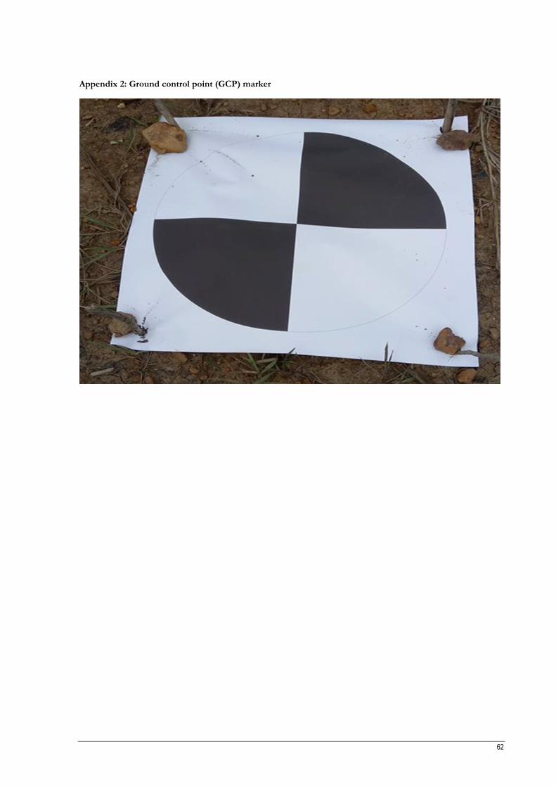
62
Appendix 2: Ground control point (GCP) marker
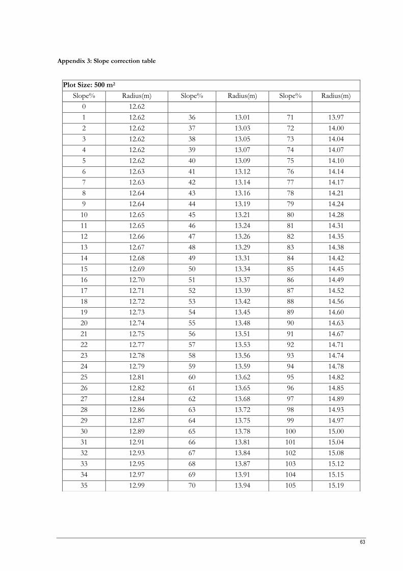
63
Appendix 3: Slope correction table
Plot Size: 500 m2
Slope% Radius(m) Slope% Radius(m) Slope% Radius(m)
0 12.62
1 12.62 36 13.01 71 13.97
2 12.62 37 13.03 72 14.00
3 12.62 38 13.05 73 14.04
4 12.62 39 13.07 74 14.07
5 12.62 40 13.09 75 14.10
6 12.63 41 13.12 76 14.14
7 12.63 42 13.14 77 14.17
8 12.64 43 13.16 78 14.21
9 12.64 44 13.19 79 14.24
10 12.65 45 13.21 80 14.28
11 12.65 46 13.24 81 14.31
12 12.66 47 13.26 82 14.35
13 12.67 48 13.29 83 14.38
14 12.68 49 13.31 84 14.42
15 12.69 50 13.34 85 14.45
16 12.70 51 13.37 86 14.49
17 12.71 52 13.39 87 14.52
18 12.72 53 13.42 88 14.56
19 12.73 54 13.45 89 14.60
20 12.74 55 13.48 90 14.63
21 12.75 56 13.51 91 14.67
22 12.77 57 13.53 92 14.71
23 12.78 58 13.56 93 14.74
24 12.79 59 13.59 94 14.78
25 12.81 60 13.62 95 14.82
26 12.82 61 13.65 96 14.85
27 12.84 62 13.68 97 14.89
28 12.86 63 13.72 98 14.93
29 12.87 64 13.75 99 14.97
30 12.89 65 13.78 100 15.00
31 12.91 66 13.81 101 15.04
32 12.93 67 13.84 102 15.08
33 12.95 68 13.87 103 15.12
34 12.97 69 13.91 104 15.15
35 12.99 70 13.94 105 15.19
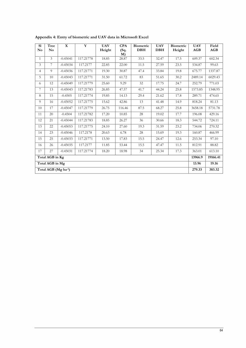
64
Appendix 4: Entry of biometric and UAV data in Microsoft Excel
Sl No
Tree No
X Y UAV Height
CPA (Sq. M)
Biometric DBH
UAV DBH
Biometric Height
UAV AGB
Field AGB
1 3 -0.45041 117.21778 18.85 28.87 33.5 32.47 17.5 609.37 602.34
3 7 -0.45034 117.2177 22.85 22.00 11.5 27.59 23.5 534.87 99.63
4 9 -0.45036 117.21771 19.30 30.87 47.4 33.84 19.8 675.77 1337.87
5 10 -0.45043 117.21771 31.50 61.72 83 51.65 30.2 2489.14 6029.43
6 12 -0.45049 117.21779 25.60 9.29 32 17.75 24.7 252.79 771.03
7 13 -0.45043 117.21783 26.85 47.57 41.7 44.24 25.8 1573.85 1348.95
8 15 -0.4505 117.21774 19.85 14.13 29.4 21.62 17.8 289.71 474.65
9 16 -0.45052 117.21775 15.62 42.86 13 41.48 14.9 818.24 81.13
10 17 -0.45047 117.21779 26.75 116.46 87.5 68.27 25.8 3658.18 5731.78
11 20 -0.4504 117.21782 17.20 10.85 28 19.02 17.7 196.08 429.16
12 21 -0.45044 117.21783 18.85 26.27 36 30.66 18.3 544.72 724.11
13 22 -0.45053 117.21775 24.10 27.60 19.3 31.59 23.2 734.06 270.32
14 23 -0.45046 117.2178 20.63 6.78 28 15.69 19.3 160.87 466.99
15 25 -0.45033 117.21771 13.50 17.83 15.5 24.47 12.6 253.34 97.10
16 26 -0.45035 117.2177 11.85 53.44 15.5 47.47 11.5 812.91 88.82
17 27 -0.45031 117.21774 18.20 18.98 34 25.34 17.3 363.01 613.10
Total AGB in Kg 13966.9 19166.41
Total AGB in Mg 13.96 19.16
Total AGB (Mg ha-1) 279.33 383.32
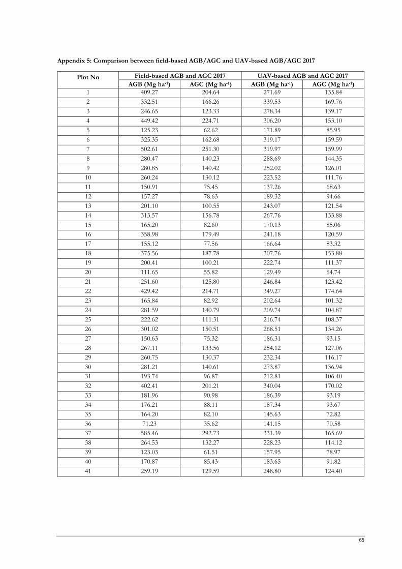
65
Appendix 5: Comparison between field-based AGB/AGC and UAV-based AGB/AGC 2017
Plot No Field-based AGB and AGC 2017 UAV-based AGB and AGC 2017
AGB (Mg ha-1) AGC (Mg ha-1) AGB (Mg ha-1) AGC (Mg ha-1)
1 409.27 204.64 271.69 135.84
2 332.51 166.26 339.53 169.76
3 246.65 123.33 278.34 139.17
4 449.42 224.71 306.20 153.10
5 125.23 62.62 171.89 85.95
6 325.35 162.68 319.17 159.59
7 502.61 251.30 319.97 159.99
8 280.47 140.23 288.69 144.35
9 280.85 140.42 252.02 126.01
10 260.24 130.12 223.52 111.76
11 150.91 75.45 137.26 68.63
12 157.27 78.63 189.32 94.66
13 201.10 100.55 243.07 121.54
14 313.57 156.78 267.76 133.88
15 165.20 82.60 170.13 85.06
16 358.98 179.49 241.18 120.59
17 155.12 77.56 166.64 83.32
18 375.56 187.78 307.76 153.88
19 200.41 100.21 222.74 111.37
20 111.65 55.82 129.49 64.74
21 251.60 125.80 246.84 123.42
22 429.42 214.71 349.27 174.64
23 165.84 82.92 202.64 101.32
24 281.59 140.79 209.74 104.87
25 222.62 111.31 216.74 108.37
26 301.02 150.51 268.51 134.26
27 150.63 75.32 186.31 93.15
28 267.11 133.56 254.12 127.06
29 260.75 130.37 232.34 116.17
30 281.21 140.61 273.87 136.94
31 193.74 96.87 212.81 106.40
32 402.41 201.21 340.04 170.02
33 181.96 90.98 186.39 93.19
34 176.21 88.11 187.34 93.67
35 164.20 82.10 145.63 72.82
36 71.23 35.62 141.15 70.58
37 585.46 292.73 331.39 165.69
38 264.53 132.27 228.23 114.12
39 123.03 61.51 157.95 78.97
40 170.87 85.43 183.65 91.82
41 259.19 129.59 248.80 124.40
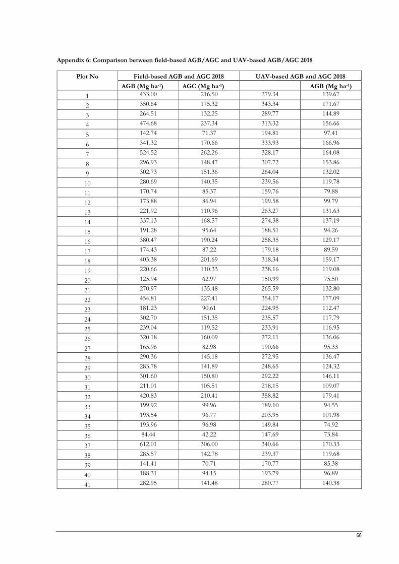
66
Appendix 6: Comparison between field-based AGB/AGC and UAV-based AGB/AGC 2018
Plot No Field-based AGB and AGC 2018 UAV-based AGB and AGC 2018
AGB (Mg ha-1) AGC (Mg ha-1) AGB (Mg ha-1)
1 433.00 216.50 279.34 139.67
2 350.64 175.32 343.34 171.67
3 264.51 132.25 289.77 144.89
4 474.68 237.34 313.32 156.66
5 142.74 71.37 194.81 97.41
6 341.32 170.66 333.93 166.96
7 524.52 262.26 328.17 164.08
8 296.93 148.47 307.72 153.86
9 302.73 151.36 264.04 132.02
10 280.69 140.35 239.56 119.78
11 170.74 85.37 159.76 79.88
12 173.88 86.94 199.58 99.79
13 221.92 110.96 263.27 131.63
14 337.13 168.57 274.38 137.19
15 191.28 95.64 188.51 94.26
16 380.47 190.24 258.35 129.17
17 174.43 87.22 179.18 89.59
18 403.38 201.69 318.34 159.17
19 220.66 110.33 238.16 119.08
20 125.94 62.97 150.99 75.50
21 270.97 135.48 265.59 132.80
22 454.81 227.41 354.17 177.09
23 181.23 90.61 224.95 112.47
24 302.70 151.35 235.57 117.79
25 239.04 119.52 233.91 116.95
26 320.18 160.09 272.11 136.06
27 165.96 82.98 190.66 95.33
28 290.36 145.18 272.95 136.47
29 283.78 141.89 248.65 124.32
30 301.60 150.80 292.22 146.11
31 211.01 105.51 218.15 109.07
32 420.83 210.41 358.82 179.41
33 199.92 99.96 189.10 94.55
34 193.54 96.77 203.95 101.98
35 193.96 96.98 149.84 74.92
36 84.44 42.22 147.69 73.84
37 612.01 306.00 340.66 170.33
38 285.57 142.78 239.37 119.68
39 141.41 70.71 170.77 85.38
40 188.31 94.15 193.79 96.89
41 282.95 141.48 280.77 140.38