Estimation methods for Value at Risk

1 Introduction

1.1 History of VaR

In the last few decades, risk managers have truly experienced a revolution. The rapid increase inthe usage of risk management techniques has spread well beyond derivatives and is totally changingthe way institutions approach their financial risk. In response to the financial disasters of the early1990s a new method called VaR (Value at Risk) was developed as a simple method to quantifymarket risk (In recent years, VaR has been used in many other areas of risk including credit riskand operational risk). Some of the financial disasters of the early 1990s are:

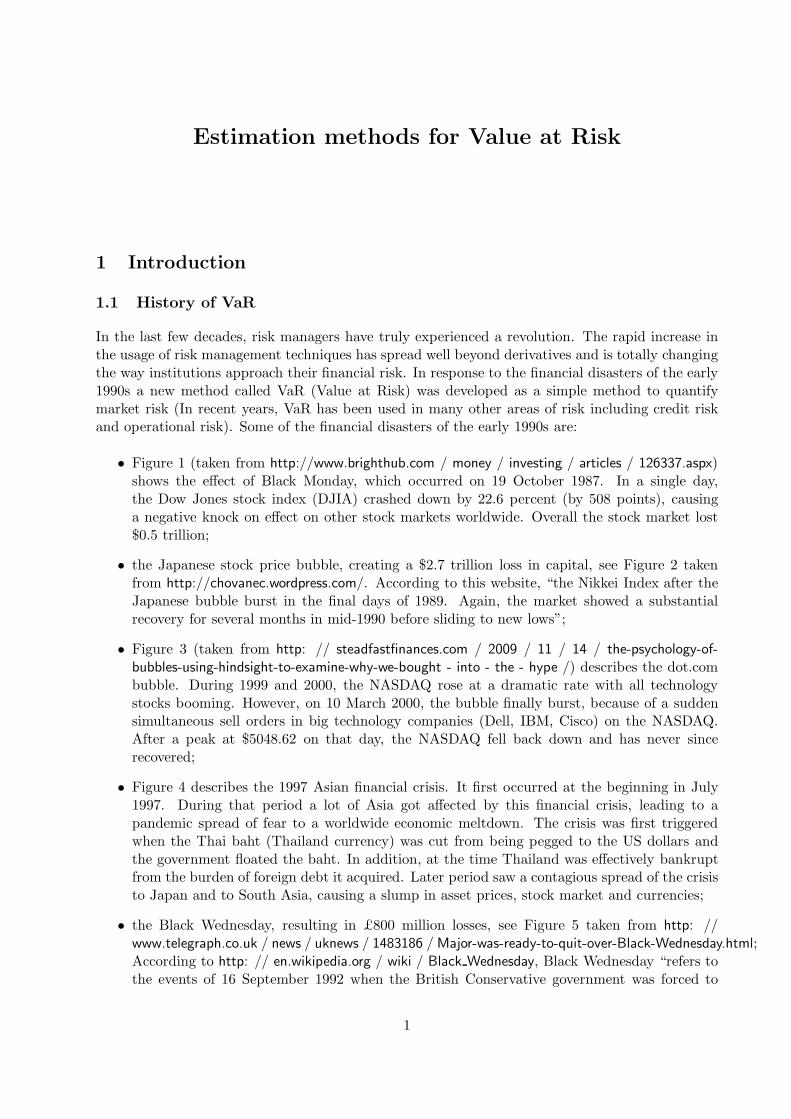
• Figure 1 (taken from http://www.brighthub.com / money / investing / articles / 126337.aspx)shows the effect of Black Monday, which occurred on 19 October 1987. In a single day,the Dow Jones stock index (DJIA) crashed down by 22.6 percent (by 508 points), causinga negative knock on effect on other stock markets worldwide. Overall the stock market lost$0.5 trillion;

• the Japanese stock price bubble, creating a $2.7 trillion loss in capital, see Figure 2 takenfrom http://chovanec.wordpress.com/. According to this website, “the Nikkei Index after theJapanese bubble burst in the final days of 1989. Again, the market showed a substantialrecovery for several months in mid-1990 before sliding to new lows”;

• Figure 3 (taken from http: // steadfastfinances.com / 2009 / 11 / 14 / the-psychology-of-bubbles-using-hindsight-to-examine-why-we-bought - into - the - hype /) describes the dot.combubble. During 1999 and 2000, the NASDAQ rose at a dramatic rate with all technologystocks booming. However, on 10 March 2000, the bubble finally burst, because of a suddensimultaneous sell orders in big technology companies (Dell, IBM, Cisco) on the NASDAQ.After a peak at $5048.62 on that day, the NASDAQ fell back down and has never sincerecovered;

• Figure 4 describes the 1997 Asian financial crisis. It first occurred at the beginning in July1997. During that period a lot of Asia got affected by this financial crisis, leading to apandemic spread of fear to a worldwide economic meltdown. The crisis was first triggeredwhen the Thai baht (Thailand currency) was cut from being pegged to the US dollars andthe government floated the baht. In addition, at the time Thailand was effectively bankruptfrom the burden of foreign debt it acquired. Later period saw a contagious spread of the crisisto Japan and to South Asia, causing a slump in asset prices, stock market and currencies;

• the Black Wednesday, resulting in £800 million losses, see Figure 5 taken from http: //www.telegraph.co.uk / news / uknews / 1483186 / Major-was-ready-to-quit-over-Black-Wednesday.html;According to http: // en.wikipedia.org / wiki / Black Wednesday, Black Wednesday “refers tothe events of 16 September 1992 when the British Conservative government was forced to

1

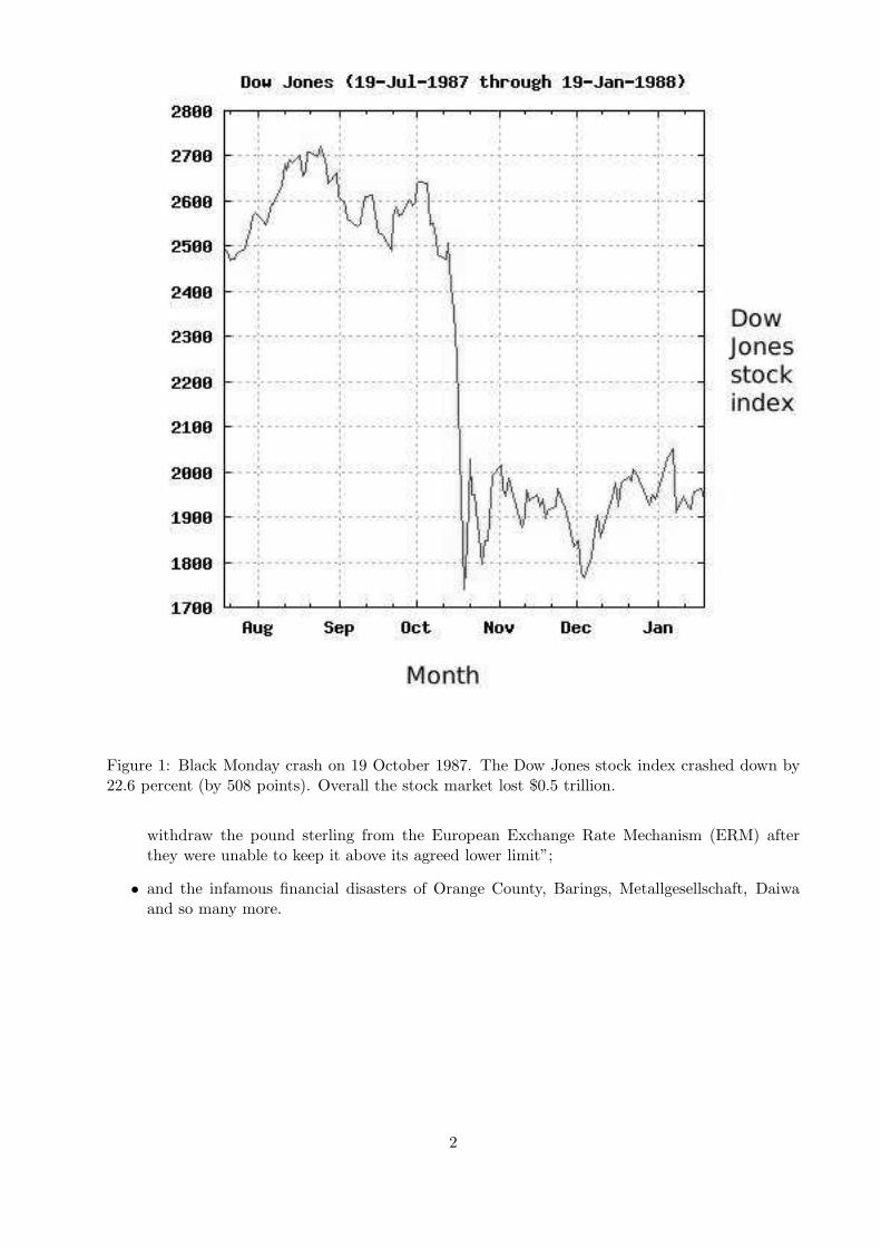
Figure 1: Black Monday crash on 19 October 1987. The Dow Jones stock index crashed down by22.6 percent (by 508 points). Overall the stock market lost $0.5 trillion.

withdraw the pound sterling from the European Exchange Rate Mechanism (ERM) afterthey were unable to keep it above its agreed lower limit”;

• and the infamous financial disasters of Orange County, Barings, Metallgesellschaft, Daiwaand so many more.

2

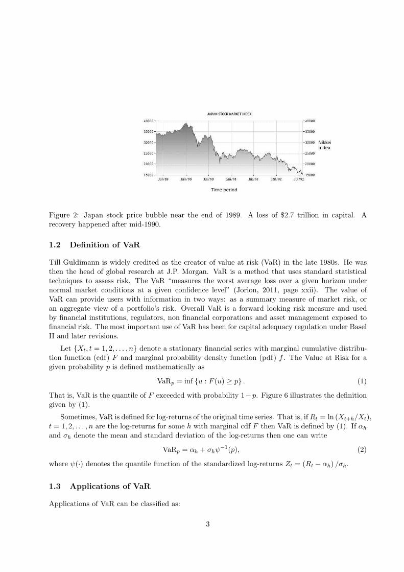
Figure 2: Japan stock price bubble near the end of 1989. A loss of $2.7 trillion in capital. Arecovery happened after mid-1990.

1.2 Definition of VaR

Till Guldimann is widely credited as the creator of value at risk (VaR) in the late 1980s. He wasthen the head of global research at J.P. Morgan. VaR is a method that uses standard statisticaltechniques to assess risk. The VaR “measures the worst average loss over a given horizon undernormal market conditions at a given confidence level” (Jorion, 2011, page xxii). The value ofVaR can provide users with information in two ways: as a summary measure of market risk, oran aggregate view of a portfolio’s risk. Overall VaR is a forward looking risk measure and usedby financial institutions, regulators, non financial corporations and asset management exposed tofinancial risk. The most important use of VaR has been for capital adequacy regulation under BaselII and later revisions.

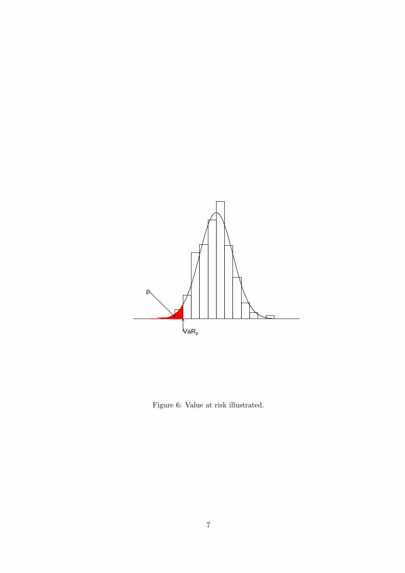
Let Xt, t = 1, 2, . . . , n denote a stationary financial series with marginal cumulative distribu-tion function (cdf) F and marginal probability density function (pdf) f . The Value at Risk for agiven probability p is defined mathematically as

VaRp = inf u : F (u) ≥ p . (1)

That is, VaR is the quantile of F exceeded with probability 1−p. Figure 6 illustrates the definitiongiven by (1).

Sometimes, VaR is defined for log-returns of the original time series. That is, ifRt = ln (Xt+h/Xt),t = 1, 2, . . . , n are the log-returns for some h with marginal cdf F then VaR is defined by (1). If αh

and σh denote the mean and standard deviation of the log-returns then one can write

VaRp = αh + σhψ−1(p), (2)

where ψ(·) denotes the quantile function of the standardized log-returns Zt = (Rt − αh) /σh.

1.3 Applications of VaR

Applications of VaR can be classified as:

3

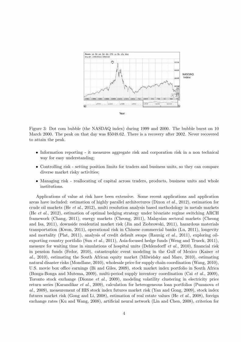
Figure 3: Dot com bubble (the NASDAQ index) during 1999 and 2000. The bubble burst on 10March 2000. The peak on that day was $5048.62. There is a recovery after 2002. Never recoveredto attain the peak.

• Information reporting - it measures aggregate risk and corporation risk in a non technicalway for easy understanding;

• Controlling risk - setting position limits for traders and business units, so they can comparediverse market risky activities;

• Managing risk - reallocating of capital across traders, products, business units and wholeinstitutions.

Applications of value at risk have been extensive. Some recent applications and applicationareas have included: estimation of highly parallel architectures (Dixon et al., 2012), estimation forcrude oil markets (He et al., 2012), multi resolution analysis based methodology in metals markets(He et al., 2012), estimation of optimal hedging strategy under bivariate regime switching ARCHframework (Chang, 2011), energy markets (Cheong, 2011), Malaysian sectoral markets (Cheongand Isa, 2011), downside residential market risk (Jin and Ziobrowski, 2011), hazardous materialstransportation (Kwon, 2011), operational risk in Chinese commercial banks (Lu, 2011), longevityand mortality (Plat, 2011), analysis of credit default swaps (Raunig et al., 2011), exploring oil-exporting country portfolio (Sun et al., 2011), Asia-focused hedge funds (Weng and Trueck, 2011),measure for waiting time in simulations of hospital units (Dehlendorff et al., 2010), financial riskin pension funds (Fedor, 2010), catastrophic event modeling in the Gulf of Mexico (Kaiser etal., 2010), estimating the South African equity market (Milwidsky and Mare, 2010), estimatingnatural disaster risks (Mondlane, 2010), wholesale price for supply chain coordination (Wang, 2010),U.S. movie box office earnings (Bi and Giles, 2009), stock market index portfolio in South Africa(Bonga-Bonga and Mutema, 2009), multi-period supply inventory coordination (Cai et al., 2009),Toronto stock exchange (Dionne et al., 2009), modeling volatility clustering in electricity pricereturn series (Karandikar et al., 2009), calculation for heterogeneous loan portfolios (Puzanova etal., 2009), measurement of HIS stock index futures market risk (Yan and Gong, 2009), stock indexfutures market risk (Gong and Li, 2008), estimation of real estate values (He et al., 2008), foreignexchange rates (Ku and Wang, 2008), artificial neural network (Lin and Chen, 2008), criterion for

4

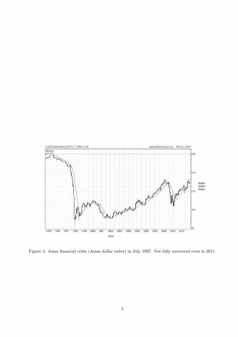
Figure 4: Asian financial crisis (Asian dollar index) in July 1997. Not fully recovered even in 2011.

5

Figure 5: Black Wednesday crash of 16 September 1992. Top image shows the exchange rate ofDeutsche mark to British pounds. Bottom image shows the UK interest rate on the day.

6

VaRp

p

Figure 6: Value at risk illustrated.

7

management of storm-water (Piantadosi et al., 2008), inventory control in supply chains (Yiu et al.,2008), layers of protection analysis (Fang et al., 2007), project finance transactions (Gatti et al.,2007), storms in the Gulf of Mexico (Kaiser et al., 2007), mid-term generation operation planningin electricity market environment (Lu et al., 2007), Hong Kong’s fiscal policy (Porter, 2007), bakeryprocurement (Wilson et al., 2007), newsvendor models (Xu and Chen, 2007), optimal allocationof uncertain water supplies (Yamout et al., 2007), futures floor trading (Lee and Locke, 2006),estimating a listed firm in China (Liu et al., 2006), Asian pacific stock market (Su and Knowles,2006), Polish power exchange (Trzpiot and Ganczarek, 2006), single loss approximation to valueat risk (Bocker and Kluppelberg, 2005), real options in complex engineered systems (Hassan etal., 2005), effects of bank technical sophistication and learning over time (Liu et al., 2004), riskanalysis of the aerospace sector (Mattedi et al., 2004), Chinese securities market (Li et al., 2002),risk management of investment-linked household property insurance (Zhu and Gao, 2002), projectrisk measurement (Feng and Chen, 2001), long-term capital management for property/casualtyinsurers (Panning, 1999), structure-dependent securities and FX derivatives (Singh, 1997), andmortgage backed securities (Jakobsen, 1996).

1.4 Aims

The aim of this lecture notes is to review known methods for estimating VaR given by (1). Thereview of methods is divided as follows: general properties (Section 2), parametric methods (Sec-tion 3), nonparametric methods (Section 4), semiparametric methods (Section 5), and computersoftware (Section 6). For each estimation method, we give the main formulas for computing valueat risk. We have avoided giving full details for each estimation method (for example, interpretation,asymptotic properties, finite sample properties, finite sample bias, sensitivity to outliers, quality ofapproximations, comparison with competing estimators, advantages, disadvantages and applicationareas) because of space concerns. These details can be read from the cited references.

1.5 Further material

The review of value of risk presented here is not complete, but we believe we have covered mostof the developments in recent years. For a fuller account of the theory and applications of valuerisk, we refer the readers to the following books: Bouchaud and Potters (2000, Chapter 3), Delbaen(2000, Chapter 3), Moix (2001, Chapter 6), Voit (2001, Chapter 7), Dupacova et al. (2002, Part2), Dash (2004, Part IV), Franke et al. (2004), Tapiero (2004, Chapter 10), Meucci (2005), Pflugand Romisch (2007, Chapter 12), Resnick (2007), Ardia (2008, Chapter 6), Franke et al. (2008),Klugman et al. (2008), Lai and Xing (2008, Chapter 12), Taniguchi et al. (2008), Janssen et al.(2009, Chapter 18), Sriboonchitta et al. (2010, Chapter 4), Tsay (2010), Capinski and Zastawniak(2011), Jorion (2011), and Ruppert (2011, Chapter 19).

2 General properties

This section describes general properties of value at risk. The properties discussed are: orderingproperties (Section 2.1), upper comonotonicity (Section 2.2), multivariate extension (Section 2.3),risk concentration (Section 2.4), Hurlimann’s inequalities (Section 2.5), Ibragimov and Walden’sinequalities (Section 2.6), Denis et al.’s inequalities (Section 2.7), Jaworski’s inequalities (Section2.8), Mesfioui and Quessy’s inequalities (Section 2.9) and Slim et al.’s inequalities (Section 2.10).

8

2.1 Ordering properties

Pflug (2000) and Jadhav and Ramanathan (2009) establish several ordering properties of VaRp.Given random variables X, Y , Y1, Y2 and a constant c, some of the properties given by Pflug (2000)and Jadhav and Ramanathan (2009) are:

(i) VaRp is translation equivariant, that is VaRp(Y + c) = VaRp(Y ) + c;

(ii) VaRp is positively homogeneous, that is VaRp(cY ) = cVaRp(Y ) for c > 0;

(iii) VaRp(Y ) = −VaR1−p(−Y );

(iv) VaRp is monotonic with respect to stochastic dominance of order 1 (a random variable Y1 isless than a random variable Y2 with respect to stochastic dominance of order 1 if E [ψ (Y1)] ≤E [ψ (Y2)] for all monotonic integrable functions ψ); that is, Y1 is less than a random variableY2 with respect to stochastic dominance of order 1 then VaRp (Y1) ≤ VaRp (Y2);

(v) VaRp is comonotone additive, that is if Y1 and Y2 are comonotone then VaRp (Y1 + Y2) =VaRp (Y1)+VaRp (Y2). Two random variables Y1 and Y2 defined on the same probability space

(Ω,A, P ) are said to be comonotone if for all w,w′ ∈ Ω, [Y1(w)− Y2(w)]

[Y1

(w

′

)− Y2

(w

′

)]≥

0 almost surely;

(vi) if X ≥ 0 then VaRp(X) ≥ 0;

(vii) VaRp is monotonic, that is if X ≥ Y then VaRp(X) ≥ VaRp(Y ).

Let F denote the joint cdf of (X1,X2) with marginal cdfs F1 and F2. Write F ≡ (F1, F2, C) tomean F (X1,X2) ≡ C (F1 (X1) , F2 (X2)), where C is known as the copula (Nelsen, 1999), a joint

cdf of uniform marginals. Let (X1,X2) have the joint cdf F ≡ (F1, F2, C),(X

′

1,X′

2

)have the joint

cdf F′ ≡

(F1, F2, C

′

), X = wX1 + (1− w)X2, and X

′

= wX′

1 + (1− w)X′

2. Then, Tsafack (2009)

shows that if C′

is stochastically less than C then VaRp

(X

′

)≥ VaRp(X) for p ∈ (0, 1).

2.2 Upper comonotonicity

If two or more assets are comonotonic then their values (whether they be small, medium, large, etc)move in the same direction simultaneously. In the real world, this may be too strong of a relation.A more realistic relation is to say that the assets move in the same direction if their values areextremely large. This weaker relation is known as upper comonotonicity (Cheung, 2009).

Let Xi denote the loss of the ith asset. Let X = (X1, . . . ,Xn) with joint cdf F (x1, . . . , xn). LetT = X1 + · · · +Xn. Suppose all random variables are defined on the probability space (Ω,F ,Pr).Then, a simple formula for the value at risk of T in terms of values at risk of Xi can be establishedif X is upper comonotonic.

We now define what is meant by upper comonotonicity. A subset C ⊂ Rn is said to be comono-

tonic if (ti − si) (tj − sj) ≥ 0 for all i and j whenever (t1, . . . , tn) and (s1, . . . , sn) belong to C. Therandom vector is said to be comonotonic if it has a comonotonic support.

Let N denote the collection of all zero probability sets in the probability space. Let Rn =Rn∪(−∞, . . . ,−∞). For a given (a1, . . . , an) ∈ R

n, let U(a) denote the upper quadrant of (a1,∞)×

9

· · · × (an,∞) and let L(a) denote the lower quadrant of (−∞, a1] × · · · × (−∞, an]. Let R(a) =Rn\ (U (a) ∪ L (a)).

Then, the random vector X is said to be upper comonotonic if there exist a ∈ Rn and a zeroprobability set N(a) ∈ N such that

(a) X(w) | w ∈ Ω\N(a) ∩ U(a) is a comonotonic subset of Rn;

(b) Pr (X ∈ U(a)) > 0;

(c) X(w) | w ∈ Ω\N(a) ∩R(a) is an empty set.

If these three conditions are satisfied then the value at risk of T can be expressed as

VaRp(T ) =

n∑

i=1

VaRp (Xi) (3)

for p ∈ (F (a∗1, . . . , a∗n) , 1) and a∗ = (a∗1, . . . , a

∗n), a comonotonic threshold as constructed in Lemma

2 of Cheung (2009).

2.3 Multivariate extension

Multivariate VaR is a much more recent topic.

Let X be a random vector in Rr with joint cdf F . Prekopa (2012) gives the following definition

of multivariate VaR:

MVaRp =u ∈ R

r∣∣∣F (u) = p

. (4)

Note that MVaR may not be a single vector. It will often take the form of a set of vectors.

Prekopa (2012) gives the following motivation for multivariate VaR: “A finance company gen-erally faces the problem of constructing different portfolios that they can sell to customers. Eachportfolio produces a random total return and it is the objective of the company to have them abovegiven levels, simultaneously, with large probability. Equivalently, the losses should be below givenlevels, with large probability. In order to ensure it we look at the total losses as components ofa random vector and find a multivariate p-quantile or MVaR to know what are those points inthe r-dimensional space (r being the number of portfolios), that should surpass the vector of totallosses, to guarantee the given reliability”.

Cousin and Bernardinoy (2011) provide another definition of multivariate VaR:

MVaRp = E [X | X ∈ ∂L(p)] =

E [X1 | X ∈ ∂L(p)]E [X2 | X ∈ ∂L(p)]

...E [Xr | X ∈ ∂L(p)]

or equivalently

MVaRp = E [X | F (X) = p] =

E [X1 | F (X) = p]E [X2 | F (X) = p]

...E [Xr | F (X) = p]

,

10

where ∂L(p) is the boundary of the setx ∈ R

r+ : F (x) ≥ p

.

Cousin and Bernardinoy (2011) establish various properties of MVaR similar to those in theunivariate case. For instance,

(i) the translation equivariant property holds, that is

MVaRp (c+X) = c+MVaRp (X) =

c1 + E [X1 | F (X) = p]c2 + E [X2 | F (X) = p]

...cr + E [Xr | F (X) = p]

;

(ii) the positively homogeneous property holds, that is

MVaRp (cX) = cMVaRp (X) =

c1E [X1 | F (X) = p]c2E [X2 | F (X) = p]

...crE [Xr | F (X) = p]

;

(iii) if F is quasi-concave (Nelson, 1999) then

MVaRip(X) ≥ VaRp (Xi)

for i = 1, 2, . . . , r, where MVaRip(X) denotes the ith component of MVaRp(X);

(iv) if X is a comonotone non-negative random vector and if F is quasi-concave (Nelson, 1999)then

MVaRip(X) = VaRp (Xi)

for i = 1, 2, . . . , r;

(v) if Xi = Yi in distribution for every i = 1, 2, . . . , s then

MVaRp(X) = MVaRp (Y)

for all p ∈ (0, 1);

(vi) if Xi is stochastically less than Yi for every i = 1, 2, . . . , s then

MVaRp(X) ≤ MVaRp (Y)

for all p ∈ (0, 1).

Bivariate value at risk in the context of a bivariate normal distribution has been consideredmuch earlier by Arbia (2002).

A matric variate extension of VaR and its application for power supply networks are discussedin Chang (2011).

11

2.4 Risk concentration

Let X1,X2, . . . ,Xn denote future losses, assumed to be non-negative independent random variableswith common cdf F and survival function F . Degen et al. (2010) define risk concentration as

C(α) =

VaRα

[n∑

i=1

Xi

]

n∑

i=1

VaRα (Xi)

.

If F is regularly varying with index−1/ξ, ξ > 0 (Bingham et al., 1989), meaning that F (tx)/F (t) →x−1/ξ as t→ ∞, then it is shown that

C(α) → nξ−1 (5)

as α→ 1. Degen et al. (2010) also study the rate of convergence in (5).

Suppose Xi, i = 1, 2, . . . , n are regularly varying with index −β, β > 0. According to Jang andJho (2007), for β > 1,

C(α) < 1

for all α ∈ [α0, 1] for some α0 ∈ (0, 1). This property is referred to as subadditivity. If C(α) < 1holds as α→ 1 then the property is referred to as asymptotic subadditivity. For β = 1,

C(α) → 1

as α→ 1. This property is referred to as asymptotic comonotonicity. For 0 < β < 1,

C(α) > 1

for all α ∈ [α0, 1] for some α0 ∈ (0, 1). If C(α) > 1 holds as α→ 1 then the property is referred toas asymptotic superadditivity.

Let N(t) denote a counting process independent of Xi with E [N(t)] <∞ for t > 0. Accordingto Jang and Jho (2007), in the case of subadditivity,

VaRα

N(t)∑

i=1

Xi

≤ E [N(t)]

N(t)∑

i=1

VaRα (Xi)

for all α ∈ [α0, 1] for some α0 ∈ (0, 1). In the case of asymptotic comonotonicity,

VaRα

N(t)∑

i=1

Xi

∼ E [N(t)]

N(t)∑

i=1

VaRα (Xi)

as α→ 1. In the case of superadditivity,

VaRα

N(t)∑

i=1

Xi

≥ E [N(t)]

N(t)∑

i=1

VaRα (Xi)

12

for all α ∈ [α0, 1] for some α0 ∈ (0, 1).

Suppose X = (X1,X2, . . . ,Xn)T is multivariate regularly varying with index β according to

Definition 2.2 in Embrechts et al. (2009). If Φ : Rn → R is a measureable function such that

limx→∞

Pr (Ψ(X) > x)

Pr (X1 > x)→ q ∈ (0,∞)

then it is shown

limα→1

VaRα (Ψ(X))

VaRα (X1)→ q1/β,

see Lemma 2.3 in Embrechts et al. (2009).

2.5 Hurlimann’s inequalities

Let X denote a random variable defined over [A,B], −∞ ≤ A < B ≤ ∞ with mean µ, and varianceσ. Hurlimann (2002) provides various upper bounds for VaRp(X): for p ≤ σ2/

σ2 + (B − µ)2

,

VaRp(X) ≤ B;

for σ2/σ2 + (B − µ)2

≤ p ≤ (µ−A)2/

σ2 + (µ−A)2

,

VaRp(X) ≤ µ+

√1− p

pσ;

for p ≥ (µ−A)2/σ2 + (µ−A)2

,

VaRp(X) ≤ µ+(µ −A)(B −A)(1 − p)− σ2

(B −A)p − (µ−A). (6)

The equality in (6) holds if and only if B → ∞.

Now suppose X is a random variable defined over [A,B], −∞ ≤ A < B ≤ ∞ with mean µ,variance σ, skewness γ and kurtosis γ2. In this case, Hurlimann (2002) provides the following upperbound for VaRp(X):

VaRp(X) ≤ µ+ xpσ,

where xp is the 100(1− p) percentile of the standardized Chebyshev-Markov maximal distribution.The latter is defined as the root of

p (xp) = p

if p ≤ (1/2)1− γ/

√4 + γ2

and as the root of

p (ψ (xp)) = 1− p

if p > (1/2)1− γ/

√4 + γ2

, where

p(u) =∆

q2(u) + ∆ (1 + u2),

ψ(u) =1

2

[A(u)−

√A2(u) + 4q(u)B(u)

q(u)

],

where ∆ = γ2 − γ2 + 2, A(u) = γq(u) + ∆u, B(u) = q(u) + ∆ and q(u) = 1 + γu− u2.

13

2.6 Ibragimov and Walden’s inequalities

Let R(w) =∑N

i=1 wiRi denote a portfolio return made up of N asset returns, Ri, and the non-negative weights wi. Ibragimov (2009) provides various inequalities for the VaR of R(w). Theysuppose that Ri are independent and identically distributed and belong to either CS, the class ofdistributions which are convolutions of symmetric stable distributions Sα(σ, 0, 0) with α ∈ (0, 1] andσ > 0 or CSLC, convolutions of distributions from the class of symmetric log-concave distributionsand the class of distributions which are convolutions of symmetric stable distributions Sα(σ, 0, 0)with α ∈ [1, 2] and σ > 0.

Here, Sα(β, γ, µ) denotes a stable distribution specified by its characteristic function

φ(t) =

expiµt− γα|t|α

[1− iβ tan

(πα

2

)sign(t)

], α 6= 1,

exp

iµt− γ|t|

(1 + iβsign(t)

2

πln t

), α = 1,

where i =√−1, α ∈ (0, 2], |β| ≤ 1, γ > 0 and µ ∈ R. The stable distribution contains as particular

cases: the Gaussian distribution for α = 2; the Cauchy distribution for α = 1, and β = 0; the Levydistribution for α = 1/2 and β = 1; the Landau distribution for α = 1 and β = 1; the dirac deltadistribution for α ↓ 0 and γ ↓ 0.

Furthermore, let IN =(w1, . . . , wN ) ∈ R

N+ : w1 + · · ·+ wN = 1

. Write a ≺ b to mean that∑k

i=1 a[i] ≤∑k

i=1 b[i] for k = 1, . . . , N−1 and∑N

i=1 a[i] =∑N

i=1 b[i], where a[1] ≥ · · · ≥ a[N ] and b[1] ≥· · · ≥ b[N ] denote the components of a and b in descending order. Let wN = (1/N, 1/N, . . . , 1/N)and wN = (1, 0, . . . , 0).

With these notation, Ibragimov (2009) provides the following inequalities for VaRq (R(w)).Suppose first that q ∈ (0, 1/2) and Ri belong to CSLC. Then,

(i) VaR1−q [R(v)] ≤ VaR1−q [R(w)] if v ≺ w;

(i) VaR1−q [R (wN )] ≤ VaR1−q [R(w)] ≤ VaR1−q [R (wN )] for all w ∈ IN .

Suppose now that q ∈ (0, 1/2) and Ri belong to CS. Then,

(i) VaR1−q [R(v)] ≥ VaR1−q [R(w)] if v ≺ w;

(i) VaR1−q [R (wN )] ≤ VaR1−q [R(w)] ≤ VaR1−q [R (wN )] for all w ∈ IN .

Further inequalities for VaR are provided in Ibragimov and Walden (2011) when a portfolioreturn, say R, is made up of a two dimensional array of asset returns say Rij . That is,

R(w) =

r∑

i=1

c∑

j=1

wijRij

=r∑

i=1

wi0Ri +r∑

i=1

w0jCj +r∑

i=1

c∑

j=1

wijUij

= R(w

(row)0

)+ C

(w

(col)0

)+ U(w),

14

where Ri, i = 1, . . . , r are referred to as “row effects”, Cj , j = 1, . . . , c are referred to as “columneffects”, and Uij , i = 1, . . . , r, j = 1, . . . , c are referred to as “idiosyncratic components”.

Let wrc = (1/(rc), 1/(rc), . . . , 1/(rc)), wrc = (1, 0, . . . , 0), w(row)0 = (1/r, 1/r, . . . , 1/r), w

(row)0 =

(1, 0, . . . , 0), w(col)0 = (1/c, 1/c, . . . , 1/c), and w

(col)0 = (1, 0, . . . , 0).

With these notation, Ibragimov and Walden (2011) provide the following inequalities for q ∈(0, 1/2):

(i) if Ri, Cj , Uij belong to CSLC then VaR1−q [R (wrc)] ≤ VaR1−q [R(w)] ≤ VaR1−q [R (wrc)]for all w ∈ Irc;

(ii) if Ri, Cj , Uij belong to CS then VaR1−q [R (wrc)] ≥ VaR1−q [R(w)] ≥ VaR1−q [R (wrc)] forall w ∈ Irc;

(iii) if Uij belong to CSLC then VaR1−q [U (wrc)] ≤ VaR1−q [U(w)] ≤ VaR1−q [U (wrc)] for allw ∈ Irc;

(iv) if Uij belong to CS then VaR1−q [U (wrc)] ≥ VaR1−q [U(w)] ≥ VaR1−q [U (wrc)] for all w ∈Irc;

(v) if Ri belong to CSLC then VaR1−q [R (wr)] ≤ VaR1−q

[R(w

(row)0

)]≤ VaR1−q [R (wr)] for

all w ∈ Irc;

(vi) if Ri belong to CS then VaR1−q [R (wr)] ≥ VaR1−q

[R(w

(row)0

)]≥ VaR1−q [R (wr)] for all

w ∈ Irc;

(vii) if Cj belong to CSLC then VaR1−q [C (wc)] ≤ VaR1−q

[C(w

(col)0

)]≤ VaR1−q [C (wc)] for

all w ∈ Irc;

(viii) if Cj belong to CS then VaR1−q [C (wc)] ≥ VaR1−q

[C(w

(col)0

)]≥ VaR1−q [C (wc)] for all

w ∈ Irc.

Ibragimov and Walden (2011, Section 4) discuss an application of these inequalities to portfoliocomponent value at risk analysis.

2.7 Denis et al.’s inequalities

Let Pt denote prices of financial assets. The process could be modeled by

Pt = m+

∫ t

0σsdBs +

∫ t

0bsds+

Nt∑

i=1

γT−

iYi,

where B is a Brownian motion, N is a compound Poisson process independent of B, T1, T2, . . . arejump times for N , b is an adapted integrable process, and σ, γ are certain random variables.

Denis et al. (2009) derive various bounds for the VaR of the process

P ∗t = sup

0≤u≤tPu.

The following assumptions are made:

15

(i) for all t > 0, E(∫ t

0 σ2sds)<∞;

(ii) jumps of the compound Poisson process are non-negative and Y1 is not identically equal tozero;

(iii) the process∑Nt

i=1 γT−

iYi for t > 0 is well defined and integrable;

(iv) the jumps have a Laplace transform, L(x) = E [exp (xY1)], x < c for c a positive constant;

(v) there exists γ∗ > 0 such that γs ≤ γ∗ almost surely for all s ∈ [0, t];

(vi) there exists b∗(t) ≥ 0 and a∗(t) ≥ 0 such that

∫ t

0σ2udu ≤ a∗(t),

∫ s

0budu ≤ b∗(t)

almost everywhere for all s ∈ [0, t]. In this case, let

Kt(δ) = δb∗(t) + δ2a∗(t)

2+ λt [L (δγ∗)− 1]

for 0 < δ < c/γ∗.

With these assumptions, Denis et al. (2009) show that

VaR1−α (P∗t ) ≤ inf

δ<c/γ∗

m+

Kt(δ)− lnα

δ

,

VaR1−α (P∗t ) ≤ inf

0<δ<c/γ∗

m+ b∗(t) +

a∗(t)δ

2+ λt

L (δγ∗)− 1

δ− lnα

δ

.

For γ ≤ 0, Denis et al. (2009) show that

VaR1−α (P∗t ) ≤ m+ b∗(t) +

√−2a∗(t) lnα.

If the jumps follow a simple Poisson process, Denis et al. (2009) show that

VaR1−α (P∗t ) ≤ inf

0<δ<∞

m+ b∗(t) +

a∗(t)δ

2+ λt

exp (δγ∗)− 1

δ− lnα

δ

.

If the jumps follow an exponential distribution with parameter ν > 0, Denis et al. (2009) showthat

VaR1−α (P∗t ) ≤ inf

0<δ<ν/γ∗

m+ b∗(t) +

a∗(t)δ

2+

λt

ν/γ∗ − δ− lnα

δ

.

About the issue of continuity / discontinuity of the market with jumps, see Walter (2015).

16

2.8 Jaworski’s inequalities

Jaworski (2007, 2008) considers the following situation: suppose si, i = 1, . . . , n are the quotientsof the currency rates at the end and at the beginning of an investment; suppose that the joint cdf of(s1, . . . , sn) is C (F1 (s1) , . . . , Fn (sn)), where C is a copula (Nelsen, 1999) and Fi is the marginal cdfof si; suppose wi is the part of the capital invested in the ith currency, where wi are non-negativeand sum to one. Then, the final investment value is

W1(w) = (w1s1 + · · ·+ wnsn)W0,

where w = (w1, . . . , wn). Jaworski (2007, 2008) defines the value of risk for a given w and aprobability α as

VaRα(w) = sup V : Pr (W0 −W1(w) ≤ V ) ≤ α .

Jaworski (2007) shows this VaR can be bounded as

n∑

i=1

VaRα′ (ei) ≤ VaRα ≤

n∑

i=1

VaRα (ei)

for portfolios consisting of only one currency, where ei = (0, . . . , 0, 1, 0, . . . , 0)T and α′

= α2/C(α, . . . , α).

2.9 Mesfioui and Quessy’s inequalities

Suppose a portfolio is made up of n assets and let X1,X2, . . . ,Xn denote the losses for the n assets.Suppose also that the joint cdf of (X1, . . . ,Xn) is C (F1 (x1) , . . . , Fn (xn)), where C is a copula(Nelsen, 1999), and Fi is the marginal cdf of Xi. Furthermore, define the dual of a given copula C(Definition 2.4, Mesfioui and Quessy, 2005) as

Cd (u1, . . . , un) = Pr (U(0, 1) ≤ u1 or · · · or U(0, 1) ≤ un) .

With these notation, Mesfioui and Quessy (2005) derive various inequalities for the value at risk ofS = X1 + · · ·+Xn. If C is such that C ≥ qCL and C ≤ Cd

U for some copulas CL and CU then

VaRα ≤ VaRα(S) ≤ VaRα,

where

VaRα = supCdU(u1,...,un)=α

n∑

i=1

F−1i (ui)

and

VaRα = infCL(u1,...,un)=α

n∑

i=1

F−1i (ui) .

If X1,X2, . . . ,Xn are identical random variables with common cdf F and if x∗ ∈ R is such thatf(x) = dF (x)/dx is non-increasing for x ≥ x∗ then it is shown under certain conditions that

VaRα(S) ≤ nF−1(δ−1CL

(α)),

17

where δCL(t) = CL(t, . . . , t) is the diagonal section of CL.

Mesfioui and Quessy (2005) also show that if X is a random variable with mean µ and varianceσ2 then

gµ,σ(α) ≤ VaRα(X) ≤ hµ,σ(α),

where

ga,b(u) = a− bq(1− u) I(u ≥ b2

a2 + b2

)

and

gha,b(u) = a+ aq2(u)I

(u ≤ b2

a2 + b2

)+ bq(u)I

(u >

b2

a2 + b2

),

where q(u) =√u/(1 − u). If Xi, i = 1, . . . , n have means µi, i = 1, . . . , n and variances σ2i ,

i = 1, . . . , n then it is shown that

gµ,σ(α) ≤ VaRα(S) ≤ hµ,σ(α),

where µ = µ1 + · · ·+ µn and σ = σ1 + · · ·+ σn.

2.10 Slim et al.’s inequalities

Suppose a portfolio is made up of d assets. Let X1,X2, . . . ,Xn denote the losses for the n assets.Let Fi and fi denote the cdf and the pdf of Xi. Let x∗i denote the value for which fi(x) isnon-increasing for all x ≤ x∗i . Given this notation, the total portfolio loss can be expressed asS = w1X1 + w2X2 + · · · + wnXn for some non-negative weights wi summing to one. Slim et al.(2010) show that the VaR of S can be bounded as follows:

VaRp ≤ VaRp(S) ≤ VaRp,

where

VaRp = infu1+···+un=α+n−1

n∑

i=1

F−1i (ui)

and

VaRp = max1≤i≤n

F

−1i (α) +

∑

1≤j 6=i≤n

F−1j (n)

for α ≤ min F1 (x∗1) , . . . , Fn (x

∗n). The use of the above results allows easy computation for

explicit VaR bounds for possibly dependent risks.

18

3 Parametric methods

This section concentrates on estimation of value at risk when data comes from a parametric dis-tribution and we want to make use of the parameters. The parametric methods summarized arebased on: Gaussian distribution (Section 3.1), Student’s t distribution (Section 3.2), Pareto pos-itive stable distribution (Section 3.3), log folded t distribution (Section 3.4), variance covariancemethod (Section 3.5), Gaussian mixture distribution (Section 3.6), generalized hyperbolic distri-bution (Section 3.7), fourier transformation method (Section 3.8), principal components method(Section 3.9), quadratic forms (Section 3.10), elliptical distribution (Section 3.11), copula method(Section 3.12), Gram-Charlier approximation (Section 3.13), delta gamma approximation (Section3.14), Cornish-Fisher approximation (Section 3.15), Johnson family method (Section 3.16), Tukeymethod (Section 3.17), asymmetric Laplace distribution (Section 3.18), asymmetric power distri-bution (Section 3.19), Weibull distribution (Section 3.20), ARCH models (Section 3.21), GARCHmodels (Section 3.22), GARCH model with heavy tails (Section 3.23), ARMA-GARCH model (Sec-tion 3.24), Markov switching ARCH model (Section 3.25), fractionally integrated GARCH model(Section 3.26), RiskMetrics model (Section 3.27), capital asset pricing model (Section 3.28), Dagumdistribution (Section 3.29), location-scale distributions (Section 3.30), discrete distributions (Sec-tion 3.31), quantile regression method (Section 3.32), Brownian motion method (Section 3.33),Bayesian method (Section 3.34), and Rachev et al.’s method (Section 3.35).

3.1 Gaussian distribution

If X1,X2, . . . ,Xn are observations from a Gaussian distribution with mean µ and variance σ2 thenVaR can be estimated by

VaRα = X +Φ−1(α)s, (7)

where X is the sample mean and s2 is the sample variance

s2 =1

n

n∑

i=1

(Xi −X

)2. (8)

The estimator in (7) is biased and consistent. If the n in (8) is replaced by n− 1 then (7) becomesunbiased and consistent.

3.2 Student’s t distribution

If X1,X2, . . . ,Xn are observations from a Student’s t distribution with ν degrees of freedom thenVaR can be estimated by (Arneric et al., 2008)

VaRα = X + tν,αs

√3 + κ

3 + 2κ,

where κ is the excess sample kurtosis and tν,α is the 100α percentile of a Student’s t random variablewith ν degrees of freedom.

19

3.3 Pareto positive stable distribution

Sarabia and Prieto (2009) and Guillen et al. (2011) introduce the Pareto positive stable distributionspecified by the cdf

F (x) = 1− exp −λ [ln(x/σ)]ν (9)

for x ≥ σ, λ > 0 and ν > 0. Here, λ and ν are shape parameters and σ is a scale parameter. ThePareto distribution is the particular case of (9) for ν = 1.

The Pareto positive stable distribution has been applied to risk management, see, for example,Guillen et al. (2011). If X is a random variable having the cdf (9) then it is easy to see that

VaRα = σ exp

[− 1

λln(1− α)

]1/ν

for 0 < α < 1. So, if(σ, λ, ν

)are maximum likelihood estimators of (σ, λ, ν) then

VaRα = σ exp

[− 1

λln(1− α)

]1/ν

for 0 < α < 1.

3.4 Log folded t distribution

Brazauskas and Kleefeld (2011) introduce the log folded t distribution specified by the quantilefunction

F−1(u) = expσQT (ν)((u+ 1)/2)

for 0 < u < 1, where σ > 0 is a scale parameter, ν > 0 is a shape parameter, and QT (ν)(·) denotesthe quantile function of a Student’s t random variable with ν degrees of freedom. Brazauskas andKleefeld (2011) also provide an application of this distribution to risk management.

Suppose X1,X2, . . . ,Xn is a random sample from the log folded t distribution with order statis-tics X1:n < X2:n < · · · < Xn:n. Brazauskas and Kleefeld (2011) show that the value at risk can beestimated by

VaR1−α = expσQT (ν)(1− α/2)

,

where

σ =

[1

n

n∑

i=1

ln2Xi

]1/2

or

σ =1

c(a, b) (n−mn −m∗n)

n−m∗

n∑

i=mn+1

lnXi:n,

where

c(a, b) =1

1− a− b

∫ 1−b

aQT (∞)((u+ 1)/2)du,

where mn and m∗n are integers 0 ≤ mn < n − m∗

n ≤ n such that mn/n → a and m∗n/n → b as

n→ ∞, where a and b are trimming proportions with 0 ≤ a+ b < 1.

20

3.5 Variance covariance method

Suppose the portfolio return, say R, is made up of N asset returns, Ri, i = 1, 2, . . . , N , as

R =

N∑

i=1

wiRi,

where wi are non-negative weights summing to one. Suppose also E (Ri) = µi, Var (Ri) = σ2i andCov (Ri, Rj) = σiσjρij . The variance covariance method suggests that the value at risk of R canbe approximated by

VaRα(R) =N∑

i=1

wiµi +Φ−1 (α)

√√√√N∑

i=1

wiσ2i +N∑

i,j=1,i 6=j

wiwjσiσjρij.

An estimator can be obtained by replacing the parameters µi, σi and ρij by their maximum likeli-hood estimators.

3.6 Gaussian mixture distribution

Let Pt denote the financial asset prices and let Rt = lnPt − lnPt−1 denote the log-return corre-sponding to the original financial series. Zhang and Cheng (2005) consider the model that Rt havea Gaussian mixture distribution specified by the pdf

f(r) =K∑

k=1

pk1√2πσk

exp

−(r − µk)

2

2σ2k

for K ≥ 1, where the mixing coefficients pk sum to one. Let VaRkα denote the VaR corresponding

to the kth component, that is

∫ VaRkα

−∞

1√2πσk

exp

−(r − µk)

2

2σ2k

dr = α.

Let VaRα denote the VaR corresponding to the mixture model, that is

∫ VaRα

−∞

K∑

k=1

pk1√2πσk

exp

−(r − µk)

2

2σ2k

dr = α.

Then, Theorem 1 in Zhang and Cheng (2005) shows that

min1≤k≤K

VaRkα ≤ VaRα ≤ max

1≤k≤KVaRk

α

always holds.

Furthermore, let αk denote the significance level of VaR corresponding to the kth component,that is

α(k) =

∫ VaR

−∞

1√2πσk

exp

−(r − µk)

2

2σ2k

dr.

21

Let α denote the significance level of VaR corresponding to the mixture model, that is

α =

∫ VaR

−∞

K∑

k=1

pk1√2πσk

exp

−(r − µk)

2

2σ2k

dr = α.

Then, Theorem 2 in Zhang and Cheng (2005) shows that

min1≤k≤K

α(k) ≤ α =

K∑

k=1

pkα(k) ≤ max

1≤k≤Kα(k)

always holds.

3.7 Generalized hyperbolic distribution

Suppose the log-returns, Rt = lnXt − lnXt−1, follow the model

Rt = σtǫt,

where σt is the volatility process and ǫt are independent and identical random variables withzero mean and unit variance. Let VaRα,t denote the corresponding value at risk. Suppose ǫt areindependent and identical and have the generalized hyperbolic distribution specified by the pdf

f(x) =(η/δ)λ√2πKλ(δη)

Kλ−1/2

(α√δ2 + (x− µ)2

)

√δ2 + (x− µ)2/α

1/2−λexp [β(x− µ)] ,

where µ ∈ R is a location parameter, α ∈ R is a shape parameter, β ∈ R is an asymmetry parameter,δ ∈ R is a scale parameter, λ ∈ R, η =

√α2 − β2, and Kν(·) denotes the modified Bessel function

of order ν.

Tian and Chan (2010) propose a method based on saddlepoint approximation for computingVaRα,t. It can be described as follows:

1. Estimate σ2t by

σ2t =

m∑

j=1

ωjRt−j

2

for m > 1, where ωj are some non-negative weights summing to one;

2. Compute t as the root of κ′(t)= t, where κ

′

(·) is defined in step 3;

3. Compute qp as the root of

p =

exp

κ(t)− tt+

1

2t2κ

′′ (t)

Φ

(−√t2κ′′

(t))

, if t > E,

1

2, if t = E,

1− exp

κ(t)− tt+

1

2t2κ

′′ (t)

Φ

(−√t2κ′′

(t))

, if t < E,

22

where

E = µ+δβKλ+1(δη)

ηKλ(δη),

κ(z) = µz + ln ηλ − λ ln η + lnKλ(δη) − lnKλ(δη),

κ′

(z) = µ+δ(β + z)Kλ+1(δη)

ηKλ(δη),

κ′′

(z) =δKλ+1(δη)

ηKλ(δη)+δ2(β + z)2Kλ+2(δη)

η2Kλ(δη)− δ2(β + z)2K2

λ+1(δη)

η2K2λ(δη)

;

4. Estimate VaRα,t by VaRα,t = σtqp.

3.8 Fourier transformation method

Siven et al. (2009) suggest a method for computing VaR by approximating the cdf F by a Fourierseries. The approximation is given by the following result due to Hughett (1998): suppose

(a) that there exists constants A and α > 1 such that F (−y) ≤ A|y|−α and 1 − F (y) ≤ A|y|−α

for all y > 0,

(b) that there exist constants B and β > 0 such that |φ(u)| ≤ B |u/(2π)|−β for all u ∈ R, whereφ(·) denotes the characteristic function corresponding to F (·);

Then, for constants 0 < l < 2/3, T > 0 and N > 0, the cdf F can be approximated as

F (x) ≈ 1

2+ 2

N/2−1∑

k=1

Re (G[k] exp (2πikx/T )) ,

where i =√−1, Re(·) denotes the real part, and

G(k) =1− cos(2πlk)

2πikφ (−2πk/T ) .

An estimator for VaRp is obtained by solving the equation

1

2+ 2

N/2−1∑

k=1

Re (G[k] exp (2πikx/T )) = p

for x.

3.9 Principal components method

Brummelhuis et al. (2002) use an approximation based on the principal component method tocompute VaR. If S(t) = (S1(t), . . . , Sn(t)) is a vector of risk factors over time t and if Π (t,S(t)) isa random variable they define VaR to be

Pr [Π (0,S(0)) −Π(t,S(t)) > VaR] = α. (10)

23

This equation is too general to be solved. So, Brummelhuis et al. (2002) consider the quadraticapproximation

Π (t,S(t)) −Π(0,S(0)) ≈ Θt+∆ξ +1

2ξΓξT

and assume that ξ is normally distributed with mean m and covariance matrix V. Under thisapproximation, we can rewrite (10) as

Pr

[Θ+∆ξ +

1

2ξΛξT ≤ −VaR

]= α.

Let V = HTH denote the Cholesky decomposition and let

Θ = Θ +m∆+1

2mΓmT ,

∆ = (∆+mΓ)HT ,

Γ = HΓHT .

Also let Γ = PDPT denote the principal components decomposition of Γ, v = ∆PD−1, and T =Θ− 1

2vDvT . With these notation, Brummelhuis et al. (2002) show that VaR can be approximatedby

VaR = K − T,

where K is the root of

1

(2π)n/2

∫

1

2zDzT≤−VaR−T

exp

−1

2|z − v|2

dz = α.

3.10 Quadratic forms

Suppose the financial series are realizations of a quadratic form

V = θ + δTY +1

2YTΛY = θ +

m∑

j=1

(δjYj +

1

2λjY

2j

),

where Y = (Y1, Y2, . . . , Ym)T is a standard normal vector, δ = (δ1, δ2, . . . , δm)T and Λ = diag(λ1, λ2, . . . , λm). Examples include non-linear positions like options in finance or the modelling ofbond prices in terms of interest rates (duration and convexity). Here, λ’s are the eigenvalues sortedin ascending order. Suppose there are n ≤ m distinct eigenvalues. Let ij denote the highest indexof the jth distinct eigenvalue with multiplicity µj . For j = 1, 2, . . . , n, let

Vj =

1

2λij

ij∑

ℓ=ij−1+1

(δℓλij

+ Yℓ

)2

, if λij 6= 0,

λij

ij∑

ℓ=ij−1+1

δℓYℓ, if λij = 0,

δ2j =

ij∑

ℓ=ij−1+1

δ2ℓ ,

a2j = δ2j/λ

2ij .

24

Let bj denote the moment generating function of V − Vj evaluated at 1/λij . With this notation,Jaschke et al. (2004) derive various approximations for VaR. The first of these applicable for λi1 < 0is

VaRα ≈ λi1 ln b1 +λi12χ2µ1,1−α

(a21),

where χ2µ,α(δ) denotes the 100α percentile of a non-central chisquare random variable with degrees

of freedom µ and non-centrality parameter δ. The second of the approximations applicable forλi1 = 0 and λin = 0 is

VaRα ≈ θ −n∑

j=2

δ2j

2λij+(F t1

)−1(α),

where

F t1(x) =

∣∣δ1∣∣

√2π

exp

−

n∑

j=2

a2j/2

n∏

j=2

∣∣∣δ21/λij∣∣∣µj/2

exp

[−x2/

(2δ

21

)]

(−x)1+∑n

j=2µj/2

.

The third of the approximations applicable for λi1 > 0 and λin < 0 is

VaRα ≈ θ −n∑

j=1

δ2j

2λij+(mα2d

)2/m,

where

d =1

Γ(m/2)

n∏

j=1

∣∣λij∣∣−µj/2 exp

−

n∑

j=1

a2j/2

.

3.11 Elliptical distribution

Suppose a portfolio return, say R, is made up of n asset returns, say Ri, i = 1, 2, . . . , n, asR = δ1R1+ · · ·+δnRn = δTR, where δi are non-negative weights summing to one, δ = (δ1, . . . , δn)

T

and R = (R1, . . . , Rn)T . Kamdem (2005) derives various expressions for the value at risk of R by

supposing that R has an elliptically symmetric distribution.

If R has the joint pdf fR(r) =| Σ |−1/2 g((r− µ)T Σ−1 (r− µ)

), where µ is the mean vector,

Σ is the variance-covariance matrix, and g(·) is a continuous and integrable function over R, thenit is shown that

VaRα(R) = δTµ+ q√δTΣδ,

where q is the root of

G(s) = α,

where

G(s) =π(n−1)/2

Γ ((n− 1)/2)

∫ −∞

s

∫ ∞

z21

(u− z21

)(n−3)/2g(u)dudz1. (11)

25

If R follows a mixture of elliptical pdfs given by

fR(r) =m∑

i=1

βj |Σj|−1/2 gj

((r− µj)

TΣ−1

j (r− µj)),

where µj is the mean vector for the jth elliptical pdf, Σj is the variance-covariance matrix for thejth elliptical pdf, and βj are non-negative weights summing to one, then it is shown that the valueat risk of R is the root of

m∑

j=1

βjGj

(δTµj +VaRα√

δTΣjδ

)= α,

where Gj(·) is defined as in (11).

3.12 Copula method

Suppose a portfolio return, say R, is made up of two asset returns, R1 and R2, as R = wR1 +(1 − w)R2, where w is the portfolio weight for asset 1 and 1 − w is the portfolio weight for asset2. Huang et al. (2009) consider computation of VaR for this situation by supposing that the jointcdf of (R1, R2) is C (F1 (R1) , F2 (R2)), where C is a copula (Nelsen, 1999), Fi is the marginal cdfof Ri and fi is the marginal pdf of Ri. Then, the cdf of R is

Pr (R ≤ r) = Pr (wR1 + (1− w)R2 ≤ r)

= Pr

(R1 ≤

r

w− (1− w)R2

w

)

=

∫ ∞

−∞

∫ r/w−(1−w)R2/w

−∞c (F1 (r1) , F2 (r2)) f1 (r1) f2 (r2) dr1dr2,

where c is the copula pdf. So, VaRp(R) can be computed by solving the equation

∫ ∞

−∞

∫ VaRp(R)/w−(1−w)R2/w

−∞C (F1 (r1) , F2 (r2)) dr1dr2 = p.

In general, this equation will have to solved numerically or by simulation.

Franke et al. (2011) consider the more general case that the portfolio return R is made up of nasset returns, Ri, i = 1, 2, . . . , n; that is

R =

n∑

i=1

wiRi

for some non-negative weights summing to one. Suppose as above that the joint cdf of (R1, . . . , Rn)is C (F1 (R1) , . . . , Fn (Rn)), where Fi is the marginal cdf of Ri and fi is the marginal pdf of Ri.Then, the cdf of R is

Pr (R ≤ r) =

∫

Uc (u1, . . . , un) du1 · · · dun,

where

U =[0, 1]n−1 × [0, un(r)]

,

26

and

un(r) = Fn

(r/wn −

n−1∑

i=1

wiF−1i (ui) /wn

).

So, VaRp(R) can be computed by solving the equation

∫

Uc (u1, . . . , un) du1 · · · dun = p.

Again, this equation will have to be computed by numerical integration or simulation.

3.13 Gram-Charlier approximation

Simonato (2011) suggests a number of approximations for computing (2). The first of these is basedon Gram Charlier expansion.

Let κ3 = E[Z3t

]denote the skewness coefficient and κ4 = E

[Z4t

]the kurtosis coefficient of the

standardized log-returns. Simonato (2011) suggests the approximation

VaRα = αh + σhψ−1GC(p),

where ψ−1GC(·) is the inverse function of

ψGC(k) = Φ(k)− κ36

(k2 − 1

)φ(k)− κ4 − 3

24k(k2 − 3

)φ(k),

where Φ(·) denotes the standard normal cdf and φ(·) denotes the standard normal pdf.

3.14 Delta gamma approximation

Let R = (R1, . . . , Rn)T denote a vector of returns normally distributed with zero means and

covariate matrix Σ. Suppose the return of an associated portfolio takes the general form Y = g(R).It will be difficult to find the value of risk of Y for general g(·). Some approximations are desirable.The delta gamma approximation is a commonly used approximation (Feuerverger and Wong, 2000).

Suppose we can approximate Y = aT1 R + RTB1R for a1 a n × 1 vector and B1 a n × nmatrix. Let Σ = HHT denote the Cholesky decomposition. Let λ1, . . . , λn and P1, . . . ,Pn denotethe eigenvalues and eigenvectors of HTB1H. Let aj denote the entries of PTHTa1, where P =(P1, . . . ,Pn). Then, the delta gamma approximation is that

Yd=

n∑

j=1

(ajZj + λjZ

2j

), (12)

where Z1, . . . , Zn are independent standard normal random variables. The value of risk can beobtained by inverting the distribution of the right hand side of (12).

27

3.15 Cornish-Fisher approximation

Another approximation suggested by Simonato (2011) is based on Cornish-Fisher expansion. Withthe notation as in Section 3.13, the approximation is

VaRα = αh + σhψ−1CF (p),

where ψ−1CF (·) is the inverse function of

ψ−1CF (p) = Φ−1(p) +

κ36

[(Φ−1(p)

)2 − 1]+κ4 − 3

24

[(Φ−1(p)

)3 − 3Φ−1(p)]

−κ23

36

[2(Φ−1(p)

)3 − 5Φ−1(p)],

where Φ−1(·) denotes the standard normal quantile function.

3.16 Johnson family method

A third approximation suggested by Simonato (2011) is based on the Johnson family of distributionsdue to Johnson (1949).

Let Y denote a standard normal random variable. A Johnson random variable can be expressedas

Z = c+ dg−1

(Y − a

b

),

where

g−1 (u) =

exp(u), for the lognormal family,[exp(u)− exp(−u)] /2, for the unbounded family,1/ [1 + exp(−u)] , for the bounded family,u, for the normal family.

Here, a, b, c and d are unknown parameters determined, for example, by the method of moments,see Hill et al. (1976).

With the notation as above, the approximation is

VaRα = αh + σhψ−1J (p; a, b, c, d),

where

ψ−1J (p; a, b, c, d) = c+ dg−1

(Φ−1(p)− a

b

),

where Φ−1(·) denotes the standard normal quantile function.

3.17 Tukey method

Jimenez and Arunachalam (2011) present a method for approximating VaR based on Tukey’s gand h family of distributions.

28

Let Y denote a standard normal random variable. A Tukey’s g and h random variable can beexpressed as

Z = g−1 [exp(gY )− 1] exp(hY 2/2

)

for g 6= 0 and h ∈ R. The family of lognormal distributions is contained as the particular case forh = 0. The family of Tukey’s h distribution is contained as the limiting case for g → 0.

With the notation as in Section 3.13, the approximation suggested by Jimenez and Arunachalam(2011) is

VaRp = A+BTg,h(Φ−1(p)

),

where A and B are location and scale parameters. For g = 0 and h = 1, Z is a normal randomvariable with mean µ and standard deviation σ, so A = µ and B = σ. For g = 0.773 andh = −0.09445, Z is an exponential random variable with parameter λ, so A = (1/λ) ln 2 andB = g/λ. For g = 0 and h = 0.057624, Z is a Student’s t random variable with ten degrees offreedom, so A = 0 and B = 1.

3.18 Asymmetric Laplace distribution

Trindade and Zhu (2007) consider the case that the log-returns of X1,X2, . . . ,Xn is a randomsample from the asymmetric Laplace distribution given by the pdf

f(x) =κ√2

τ (1 + κ2)

exp

(−κ

√2

τ|x− θ|

), if x ≥ θ,

exp

(−√2

κτ|x− θ|

), if x < θ

for x ∈ R, τ > 0 and κ > 0. The maximum likelihood estimator of VaRα is derived as

VaRα = − τ ln[(1 + κ2

)(1− α)

]

κ√2

,

where (τ , κ) are the maximum likelihood estimators of (τ, κ). Trindade and Zhu (2007) show furtherthat

√n(VaRα −VaRα

)→ N

(0, σ2

)

in distribution as n→ ∞, where σ2 = τ2[(ω − 1)2κ2 + 2ω2

]/(4κ2)and ω = ln

[(1 + κ2

)(1− α)

].

3.19 Asymmetric power distribution

Komunjer (2007) introduces the asymmetric power distribution as a model for risk management.A random variable, say X, is said to have this distribution if its pdf is

f(x) =

δ1/λ

Γ(1 + 1/λ)exp

[− δ

αλ|x|λ

], if x ≤ 0,

δ1/λ

Γ(1 + 1/λ)exp

[− δ

(1− α)λ|x|λ

], if x > 0

(13)

29

for x ∈ R, where 0 < α < 1, λ > 0 and δ = 2αλ(1 − α)λ/αλ + (1− α)λ

. Note that λ is a shape

parameter and α is a scale parameter. The cdf corresponding to (13) is shown to be (Lemma 1,Komunjer, 2007)

F (x) =

α

[1− I

(δ

αλ

√λ|x|λ, 1/λ

)], if x ≤ 0,

1− (1− α)

[1− I

(δ

(1− α)λ

√λ|x|λ, 1/λ

)], if x > 0,

(14)

where I(x, γ) =∫ x

√γ

0 tγ−1 exp(−t)dt/Γ(γ). Inverting (14) as in Lemma 2 of Komunjer (2007), wecan express VaRp(X) as

VaRp(X) =

−[αλ

δ√λ

]1/λ [I−1

(1− p

α,1

λ

)]1/λ, if p ≤ α,

−[(1− α)λ

δ√λ

]1/λ [I−1

(1− 1− p

1− α,1

λ

)]1/λ, if p > α,

(15)

where I−1(·, ·) denotes the inverse function of I(·, ·). An estimator of VaRp(X) can be obtainedby replacing the parameters in (15) by their maximum likelihood estimators, see Proposition 2 inKomunjer (2007).

3.20 Weibull distribution

Gebizlioglu et al. (2011) consider estimation of VaR based on the Weibull distribution. SupposeX1,X2, . . . ,Xn is a random sample from a Weibull distribution with the cdf specified by F (x) =1− exp

−(x/θ)β

for x > 0, θ > 0 and β > 0. Then, the estimator for VaR is

VaRα = − ln(1− α)1/β θ.

Gebizlioglu et al. (2011) consider various methods for obtaining the estimators θ and β. By themethod of maximum likelihood, θ and β are the simultaneous solutions of

x2

s2=

Γ (1 + 1/β)2Γ (1 + 2/β) − Γ2 (1 + 1/β)

and

θ =x

Γ(1 + 1/β

) ,

where x is the sample mean and s2 is the sample variance. By Cohen and Whitten (1982)’s modifiedmethod of maximum likelihood, θ and α are the simultaneous solutions of

−nXβ

(1)

ln [n/(n+ 1)]=

n∑

i=1

Xβi

and

θ =

(1

n

n∑

i=1

X βi

)1/β

,

30

where X(1) ≤ X(2) ≤ · · · ≤ X(n) are the order statistics in ascending order. By Tiku (1967, 1968)and Tiku and Akkaya (2004)’s modified method of maximum likelihood,

θ = exp(δ), β = 1/η,

where

δ = K +Dη, η =B +

√B2 + 4nC

/(2n),

K =

n∑

i=1

βiX(i)/m, D =

n∑

i=1

(αi − 1) /m,

B =

n∑

i=1

(αi − 1)(X(i) −K

), C =

n∑

i=1

βi(X(i) −K

)2,

m =n∑

i=1

βi, αi =[1− t(i)

]exp

(t(i)),

βi = exp(t(i)), t(i) = ln (− ln (1− i/(n + 1))) .

By the least squares method, θ and α are those minimizing

n∑

i=1

(1− exp

−[X(i)/θ

]β− i

n+ 1

)2

with respect to θ and α. By the weighted least squares method, θ and α are those minimizing

n∑

i=1

(n+ 1)2(n+ 2)

i(n − i+ 1)

(1− exp

−[X(i)/θ

]β− i

n+ 1

)2

with respect to θ and α. By the percentile method, θ and α are those minimizing

n∑

i=1

X(i) − θ

[− ln

(1− i

n+ 1

)]1/β2

with respect to θ and α.

3.21 ARCH models

ARCH models are popular in finance. Suppose the log-returns, say Rt, of X1,X2, . . . ,Xn followthe ARCH model specified by

Rt = σtǫt, σ2t = β0 +

k∑

j=1

βjR2t−j ,

where ǫi are independent and identical random variables with zero mean, unit variance, pdf f(·)and cdf F (·), and β = (β0, β1 . . . , βk)

T is an unknown parameter vector satisfying β0 > 0 and

βj ≥ 0, j = 1, 2, . . . , k. If β =(β0, β1 . . . , βk

)Tare the maximum likelihood estimators then the

residuals are

ǫt = Rt/σt,

31

where

σ2t = β0 +k∑

j=1

βjR2t−j.

Taniai and Taniguchi (2008) show that VaR for this ARCH model can be approximated by

VaRp ≈ σn+1

[F−1(p) + σΦ−1(α)/

√n],

where

σ2 =1

f2 (F−1(p))

[p(1− p)

+F−1(p)f(F−1(p)

)∫ F−1(p)

−∞u2f(u)du− p

τTU−1V

+1

4

(F−1(p)

)2f2(F−1(p)

)τTU−1SU−1τ

],

whereV = E[σ2tWt−1

], S = 2E

[σ4tWt−1W

Tt−1

], W =

(1, R2

t , . . . , R2t−k+1

)T, U = E

[Wt−1W

Tt−1

],

τ = (τ0, τ1, . . . , τk)T , τ0 = E

[1/σ2t

], and τj = E

[R2

t−j/σ2t

], j = 1, 2, . . . , k.

3.22 GARCH models

Suppose the financial returns, say Rt, satisfy the model

[1− φ(L)]Rt = [1− θ(L)] ǫt, ǫt = ηt√ht, (16)

where ηt are independent and identical standard normal random variables, Rt is the return at timet, L denotes the lag operator satisfying LRt = Rt−1, φ(L) is the polynomial φ(L) = 1−∑r

i=1 φiLi,

θ(L) is the polynomial θ(L) = 1+∑s

i=1 θiLi, ht is the conditional variance, and ηt are independent

and identical residuals with zero means and unit variances. One popular specification for ht is

ht = ω +

p∑

i=1

αiǫ2t−i +

q∑

i=1

βiht−i. (17)

This corresponds to the GARCH (p, q) model.

For the model given by (16) and (17), Chan (2009b) proposes the following algorithm forcomputing VaR:

1. Estimate the maximum likelihood estimates of the parameters in (16) and (17);

2. Using the parameter estimates, compute the standardized residuals ηt = (Rt − rt) /ht;

3. Compute the first k sample moments for ηt;

32

4. Compute

p (ηt) = exp

(k∑

i=1

λiηit

)/

∫exp

(k∑

i=1

λiηit

)dηt.

The parameters λ1, λ2, . . . , λk are determined from the sample moments of step 3 in a wayexplained in Chan (2009a) and Rockinger and Jondeau (2002);

5. Compute VaRp as the root of the equation

∫ K

−∞p (ηt) dηt = p.

3.23 GARCH model with heavy tails

Chan et al. (2007) consider the case that financial returns, say Rt, come from a GARCH (p, q)specified by

Rt = σtǫt, σ2t = c+

p∑

i=1

biR2t−i +

q∑

j=1

ajσ2t−j ,

where Rt is strictly stationary with ER2t < ∞, and ǫt are zero mean, unit variance, independent

and identical random variables independent of Rt−k, k ≥ 1. Further, Chan et al. (2007) assumethat ǫt have heavy tails, that is their cdf, say G, satisfies

limx→∞

1−G(xy)

1−G(x)= y−γ , lim

x→∞G(−x)1−G(x)

= d

for all y > 0, where γ > 0 and d ≥ 0. Chan et al. (2007) show that the VaR for this model givenby

VaRα = inf x : Pr (Rn+1 ≤ x|Rn+1−k, k ≥ 1) ≥ α

can be estimated by

VaRα = σn+1

(a, b, c

)(1− α)−1/γ

(k

m

)1/γ

ǫm,m−k,

33

where

σ2t (a, b, c) =c

1−q∑

j=1

aj

+

p∑

i=1

biR2t−i

+

p∑

i=1

bi

∞∑

k=1

q∑

j1=1

· · ·q∑

jk=1

aj1 · · · ajkR2t−i−j1−···−jk

I t− i− j1 − · · · − jk ≥ 1 ,

Lν(a, b, c) =

n∑

t=ν

R2

t /σ2t (a, b, c) + ln σ2t (a, b, c)

,

(a, b, c

)= argmin(a,b,c)Lν(a, b, c),

ǫt = Rt/σ2t

(a, b, c

),

γ =

1

k

k∑

i=1

lnǫm,m−i+1

ǫm,m−k

−1

,

where ν = ν(n) → ∞ and ν/n → 0 as n → ∞, m = n − ν + 1, ǫm,1 ≤ ǫm,2 ≤ · · · ≤ ǫm,m are theorder statistics of ǫν , ǫν+1, . . . , ǫn, and k = k(m) → ∞ and k/m → 0 as n→ ∞. Chan et al. (2007)

also establish asymptotic normality of VaRα.

3.24 ARMA-GARCH model

Suppose the financial returns, say Rt, t = 1, 2, . . . , T , satisfy the ARMA(p, q)-GARCH(r, s) modelspecified by

Rt = a0 +

p∑

i=1

aiRt−i + ǫt +

q∑

j=1

bjǫt−j,

σ2t = c0 +

r∑

i=1

ciǫ2t−i +

s∑

j=1

djσ2t−j ,

ǫt = ztσt,

where zt are independent standard normal random variables. For this model, Hartz et al. (2006)show that the h-step ahead forecast of value at risk can be estimated by

µT+h + σT+hΦ−1(α),

34

where

ǫt = Rt − a0 −p∑

i=1

aiRt−i −q∑

j=1

bj ǫt−j ,

σ2t = c0 +r∑

i=1

ciǫ2t−i +

s∑

j=1

dj σ2t−j ,

µT+h = a0 +

p∑

i=1

aiRT+h−i +

q∑

j=1

bj ǫT+h−j,

σ2T+h = c0 +r∑

i=1

ciǫ2T+h−i +

s∑

j=1

dj σ2T+h−j.

The parameter estimators required can be obtained, for example, by the method of maximumlikelihood.

3.25 Markov switching ARCH model

Suppose the financial returns, say Rt, t = 1, 2, . . . , T , satisfy the Markov switching ARCH modelspecified by

Rt = ust + ǫt,

ǫt = (gstwt)1/2 ,

wt = (htet)1/2 ,

ht = a0 + a1w2t−1 + · · ·+ aqw

2t−q,

where et are standard normal random variables, st is an unobservable random variable assumed tofollow a first-order Markov process, and wt is a typical ARCH (q) process. This model is due toBollerslev (1986). An estimator of the value at risk at time t can be obtained by inverting the cdfof Rt with its parameters replaced by their maximum likelihood estimators.

3.26 Fractionally integrated GARCH model

Suppose the financial returns, say Rt, t = 1, 2, . . . , T , satisfy the fractionally integrated GARCHmodel specified by

Rt = σtǫt,

σ2t = w +

p∑

i=1

βi(σ2t−i −R2

t−i

)−

∞∑

i=1

λiR2t−i,

where ǫt are random variables with zero means and unit variances. This model is due to Baillieet al. (1996). An estimator of the value at risk at time t can be obtained by inverting the cdf ofRt with its parameters replaced by their maximum likelihood estimators. This of course dependson the distribution of ǫt. If, for example, ǫt are normally distributed then VaRt,α = σt+1Φ

−1(α),where σt+1 may be the maximum likelihood estimator of σt+1.

35

3.27 RiskMetrics model

Suppose Rt are the log-returns of X1,X2, . . . ,Xn and let Ωt denote the information up to timet. The RiskMetrics model (RiskMetrics, 1996) is specified by

Rt = ǫt,

ǫt∣∣Ωt−1 ∼ N

(0, σ2t

),

σ2t = λσ2t−1 + (1− λ)ǫ2t−1, 0 < λ < 1.

The value at risk for this model can be computed by inverting

Pr (Rt < VaRt,α) = α

with the parameters, σ2t and λ, replaced by their maximum likelihood estimators.

3.28 Capital asset pricing model

Let Ri denote the return on asset i, let Rf denote the “risk-free rate”, and let Rm denote the“return on the market portfolio”. With this notation, Fernandez (2006) considers the capital assetpricing model given by

Ri −Rf = αi + βi (Rm −Rf ) ǫi

for i = 1, 2, . . . , k, where ǫi are independent random variables with Var (ǫi) = σ2ǫi , and Var (Rm) =σ2m. It is easy to see that

Var (Ri) = β2i σ2m + σ2e ,

Cov (Ri, Rj) = βiβjσ2m.

Fernandez (2006) shows that the value at risk of the portfolio of k assets can be expressed as

VaRα = V0Φ−1(α)

√wT (ββTσ2m +E)w, (18)

wherew is a k×1 vector of portfolio weights, V0 is the initial value of the portfolio, β = (β1, . . . , βk)T

and E = diag(σ2ǫ1 , . . . , σ

2ǫk

)T. An estimator of (18) can be obtained by replacing the parameters

by their maximum likelihood estimators.

3.29 Dagum distribution

The Dagnum distribution is due to Dagum (1977, 1980). It has the pdf and cdf specified by

f(x) = βλδ exp(−δx) [1 + λ exp(−δx)]−β−1

and

F (x) = [1 + λ exp(−δx)]−β ,

respectively, for x > 0, λ > 0, β > 0 and δ > 0. Domma and Perri (2009) discuss an application ofthis distribution for VaR estimation. They show that

VaRp =1

δln

(λ

p−1/β − 1

),

36

where(λ, β, δ

)are maximum likelihood estimators of (λ, β, δ) based on X1,X2, . . . ,Xn being a

random sample coming from the Dagnum distribution. Domma and Perri (2009) show further that

√n(VaRp −VaRp

)→ N

(0, σ2

)

in distribution as n→ ∞, where σ = gI−1gT and

g =

[− p−1/β ln p

δβ2(p−1/β − 1

) , 1

λδ,− 1

δ2ln

(λ

p−1/β − 1

)].

Here, I is the expected information matrix of(λ, β, δ

). An explicit expression for the matrix is

given in the appendix of Domma and Perri (2009).

3.30 Location-scale distributions

Suppose X1,X2, . . . ,Xn is a random sample from a location-scale family with cdf Fµ,σ(x) =F0 ((x− µ)/σ) and pdf fµ,σ(x). Then,

VaRp = µ+ zpσ, (19)

where zp = F−10 (p). The point estimator for VaR is

VaRp = µn + zpcnσn,

where

µn =1

n

n∑

i=1

Xi,

σ2n =1

n− 1

n∑

i=1

(Xi − µn)2 ,

and

cn = (E [σn/σ])−1 .

Bae and Iscoe (2012) propose various confidence intervals for VaR. Based on cn = 1 +O(n−1

)

and asymptotic normality, Bae and Iscoe (2012) propose the interval

µn + zpσn ± σn√nz(1+α)/2

√

1 +z2p4(κ− 1) + zpω, (20)

where α is the confidence level, κ is the kurtosis of F0(x), and ω is the skewness of F0(x). Based onBahadur (1966)’s almost sure representation of the sample quantile of a sequence of independentrandom variables, Bae and Iscoe (2012) propose the interval

ξp ±1√nz(1+α)/2

√p(1− p)

fµ,σ

(ξp

) ,

37

where ξp is the pth quantile and ξp is its sample counterpart.

Sometimes the financial series of interest is strictly positive. In this case, if X1,X2, . . . ,Xn isa random sample from a log location-scale family with cdf Gµ,σ(x) = lnF0 ((x− µ)/σ), then (19)and (20) generalize to

VaRp = exp (µ+ zpσ)

and

exp

µn + zpσn ± σn

nz(1+α)/2

√

1 +z2p4(κ− 1) + zpω

,

respectively, as noted by Bae and Iscoe (2012).

3.31 Discrete distributions

Gob (2011) considers VaR estimation for the three most common discrete distributions: Poisson,binomial and negative binomial. Let

Lc(λ) =

c∑

y=0

λy exp(−λ)y!

.

Then, the VaR for the Poisson distribution is

VaRp(λ) = inf c = 0, 1, . . . | Lc(λ) ≥ p .

Letting

Ln,c(r) =c∑

y=0

(n

y

)ry(1− r)n−y,

the VaR for the binomial distribution is

VaRp(r) = inf c = 0, 1, . . . | Ln,c(r) ≥ p .

Letting

Hn,c(r) =

c∑

y=0

(n+ y − 1

y

)(1− r)yrn,

the VaR for the negative binomial distribution is

VaRp(r) = inf c = 0, 1, . . . | Hn,c(r) ≥ p .

Gob (2011) derives various properties of these VaR measures in terms of their parameters. For thePoisson distribution, the following properties were derived:

(a) for fixed p ∈ (0, 1), VaRp(λ) is increasing in λ ∈ [0,∞) with limλ→∞VaRp(λ) = ∞. There arevalues 0 = λ−1 < λ0 < λ1 < λ2 < · · · , limc→∞ λc = ∞, such that, for c ∈ N0, VaRp(λ) = c onthe interval (λc−1, λc] and Lc(λ) > Lc (λc) = p for λ ∈ (λc−1, λc). In particular, λ0 = − ln(p).

38

(b) For fixed λ > 0, c = −1, 0, 1, . . ., let pc = Lc(λ). Then, for c = 0, 1, 2, . . ., VaRp(λ) = c forp ∈ (pc−1, pc].

For the binomial distribution, the following properties were derived:

(a) for fixed p ∈ (0, 1), VaRp(r) is increasing in r ∈ [0, 1]. There are values 0 = r−1 < r0 < r1 <r2 < · · · < rn = 1 such that, for c ∈ 0, . . . , n, VaRp(r) = c on the interval (rc−1, rc] andLn,c(r) > Ln,c (rc) = p for r ∈ (rc−1, rc). In particular, r0 = 1− p1/n and rn−1 = (1− p)1/n.

(b) For fixed 0 < r < 1, c = −1, 0, 1, . . ., let pc = Ln,c(r). Then, for c = 0, 1, 2, . . . , n, VaRp(r) = cfor p ∈ (pc−1, pc].

For the negative binomial distribution, the following properties were derived:

(a) for fixed p ∈ (0, 1), VaRp(r) is decreasing in r ∈ [0, 1]. There are values 1 = r−1 > r0 > r1 >r2 > · · · , limc→∞ rc = 0, such that, for c ∈ N0, VaRp(r) = c on the interval [rc, rc−1) andHn,c(r) > Hn,c (rc) = p for r ∈ (rc, rc−1). In particular, r0 = p1/n.

(b) For fixed 0 < r < 1, c = −1, 0, 1, . . ., let pc = Hn,c(r). Then, for c = 0, 1, 2, . . . , n, VaRp(r) = cfor p ∈ (pc−1, pc].

Empirical estimation of the three VaR measures can be based on asymptotic normality.

3.32 Quantile regression method

Quantile regressions have been used to estimate value at risk, see Koenker and Basset (1978),Koenker and Portnoy (1997), Chernozhukov and Umantsev (2001) and Engle and Manganelli(2004). The idea is to regress the value at risk on some known covariates. Let Xt at time tdenote the financial variable, let zt denote a k × 1 vector of covariates at time t, let βα denote ak× 1 vector of regression coefficients, and let VaRt,α denote the corresponding value at risk. Then,the quantile regression model can be rewritten as

VaRt,α = g (zt;βα) . (21)

In the linear case, (21) could take the form

VaRt,α = zTt βα.

The parameters in (21) can be estimated by least squares as in standard regression.

3.33 Brownian motion method

Cakir and Raei (2007) describe simulation schemes for computing value at risk for single asset andmultiple asset portfolios. Let Pt denote the price at time t, let T denote a holding period dividedinto small intervals of equal length ∆t, let ∆Pt denote the change in Pt over ∆t, let Zt denotea standard normal shock, let µ denote the mean of returns over the holding period T , and let σdenote the standard deviation of returns over the holding period T . With these notation, Cakirand Raei (2007) suggest the model

∆Pt

Pt= µ∆t+ σ

√∆tZt. (22)

Under this model, the VaR for single asset portfolios can be computed as follows:

39

(i) starting with Pt, simulate Pt, Pt+1, . . . , PT using (22);

(ii) repeat step (i) ten thousand times;

(iii) compute the empirical cdf over the holding period;

(iii) compute VaRα as 100α percentile of the empirical cdf.

The VaR for multiple asset portfolios can be computed as follows:

(i) suppose the price at time t for the ith asset follows

∆P it

P it

= µi∆t+ σi√∆tZi

t (23)

for i = 1, 2, . . . , N , where N is the number of assets, and the notation is the same as thatfor single asset portfolios. The standard normal shocks, Zi

t , i = 1, 2, . . . , N , need not becorrelated;

(ii) starting with P it , i = 1, 2, . . . , N , simulate P i

t , Pit+1, . . . , P

iT , i = 1, 2, . . . , N using (23);

(iii) compute the portfolio price for the holding period as the weighted sum of the individual assetprices;

(iv) repeat steps (ii) and (iii) ten thousand times;

(v) compute the empirical cdf of the portfolio price over the holding period;

(vi) compute VaRα as 100α percentile of the empirical cdf.

3.34 Bayesian method

Pollard (2007) defines a Bayesian value at risk. Let Xt denote the financial variable of interest attime t. Let p (Xt | Θ, Zt) denote the posterior pdf of Xt given some parameters Θ and “state”variables Zt. Pollard (2007) defines the Bayesian value at risk at time t as

VaRα =

x :

∫ x

−∞p (y | Θ, Zt+1) dy = α

. (24)

The “state” variables Zt are assumed to follow a transition pdf f (Zt, Zt+1).

Pollard (2007) also proposes several methods for estimating (24). One of them is the following:

(i) Use Markov Chain Monte Carlo to simulate N samples,(Z

(n)t ,Θ(n)

), n = 1, 2, . . . , N

,

from the joint conditional posterior pdf of (Zt,Θ) given Yt = Xτ , τ = 1, 2, . . . , t;

(ii) For n from 1 to N , simulate Z(n)t+1 from the conditional posterior pdf of Zt+1 given Θ(n) and

Z(n)t ;

(iii) For n from 1 to N , simulate X(n)t+1 from the conditional posterior pdf of Xt+1 given Θ(n) and

Z(n)t+1;

40

(iv) Compute the empirical cdf

G(x) =1

N

N∑

n=1

IX

(n)t+1 ≤ x

; (25)

(v) Estimate VaR as G−1(α).

3.35 Rachev et al.’s method

Let R =∑n

i=1 wiRi denote a portfolio return made up of n asset returns, Ri, and the non-negativeweights wi summing to one. Suppose Ri are independent Sα (αi, βi, 0) random variables. Then, itcan be shown that (Rachev et al., 2003) R ∼ Sα (αp, βp, 0), where

αp =

[n∑

i=1

(|wi|σi)α]1/α

and

βp =

n∑

i=1

sign (wi)βi (|wi|σi)α

n∑

i=1

(|wi|σi)α.

Hence, the value of risk of R can be estimated by the following algorithm due to Rachev et al.(2003):

• estimate αi and βi (to obtain say αi and βi) using possible data on the ith asset return;

• estimate αp and βp by

αp =

[n∑

i=1

(|wi| σi)α]1/α

and

βp =

n∑

i=1

sign (wi) βi (|wi| σi)α

n∑

i=1

(|wi| σi)α,

respectively;

• estimate VaRp(R) as the pth quantile of Sα

(αp, βp, 0

).

41

4 Nonparametric methods

This section concentrates on estimation methods for value at risk when the data are assumed tocome from no particular distribution. The nonparametric methods summarized are based on: his-torical method (Section 4.1), filtered historical method (Section 4.2), importance sampling method(Section 4.3), bootstrap method (Section 4.4), kernel method (Section 4.5), Chang et al.’s estima-tors (Section 4.6), Jadhav and Ramanathan’s method (Section 4.7), and Jeong and Kang’s method(Section 4.8).

4.1 Historical method

Let X(1) ≤ X(2) ≤ · · · ≤ X(n) denote the order statistics in ascending order corresponding to theoriginal financial series X1,X2, . . . ,Xn. The historical method suggests to estimate value at riskby

VaRα(X) = X(i)

for α ∈ ((i− 1)/n, i/n].

4.2 Filtered historical method

Suppose the log-returns, Rt = lnXt− lnXt−1, follow the model, Rt = σtǫt, discussed before, whereσt is the volatility process and ǫt are independent and identical random variables with zero means.Let ǫ(1) ≤ ǫ(2) ≤ · · · ≤ ǫ(n) denote the order statistics of ǫt. The filtered historical methodsuggests to estimate value at risk by

VaRα = ǫ(i)σt

for α ∈ ((i− 1)/n, i/n], where σt denotes an estimator of σt at time t. This method is due to Hulland White (1998) and Barone-Adesi et al. (1999).

4.3 Importance sampling method

Suppose F (·) is the empirical cdf of X1,X2, . . . ,Xn. As seen in Section 4.1, an estimator for VaRis F−1(α). This estimator is asymptotically normal with variance equal to

α(1 − α)

nf2 (VaRα).

This can be large if α is closer to zero or one. There are several methods for variance reduction. Onepopular method is importance sampling. Suppose G(·) is another cdf and let S(x) = F (dx)/G(dx)and

S(x) =1

n

n∑

i=1

I Xi ≤ xS (Xi) .

Hong (2011) shows that S−1(p) under certain conditions can provide estimators for VaR withsmaller variance.

42

4.4 Bootstrap method

Suppose F (·) is the empirical cdf of X1,X2, . . . ,Xn. The bootstrap method can be described asfollows:

1. simulate B independent sample from F (·);

2. for each sample estimate VaRα, say VaR(i)

α for i = 1, 2, . . . , B, using the historical method;

3. take the estimate of VaR as the mean or the median of VaR(i)

α for i = 1, 2, . . . , B.

One can also construct confidence intervals for VaR based on the bootstrapped estimates VaR(i)

α ,i = 1, 2, . . . , B.

4.5 Kernel method

Kernels are commonly used to estimate pdfs. Let K(·) denote a symmetric kernel, i.e., a symmetricpdf. The kernel estimator of F can be given by

F (x) =1

n

n∑

i=1

G

(x−Xi

h

), (26)

where h is a smoothing bandwidth and

G(x) =

∫ x

−∞K(u)du.

A variable width version of (26) is

F (x) =1

n

n∑

i=1

1

hTiG

(x−Xi

hTi

), (27)

where Ti = dk (xi) is the distance of Xi from its kth nearest neighbor among the remaining (n− 1)

data points and k = n−1/2. The kernel estimator of VaR, say VaRp, is then the root of the equation

F (x) = p (28)

for x, where F (·) is given by (26) or (27). According to Sheather and Marron (1990), VaRp couldalso be estimated by

VaRp =

n∑

i=1

F ((i− 1/2)/n − p)X(i)

n∑

i=1

F ((i− 1/2)/n − p)

,

where F (·) is given by (26) or (27) andX(i)

are the ascending order statistics of Xi.

The estimator in (28) is due to Gourieroux et al. (2000). Its properties have been studied manyauthors. For instance, Chen and Tang (2005) show under certain regularity conditions that

√n(VaRp −VaRp

)→ N

(0, σ2(p)f−2 (VaRp)

)

43

in distribution as n→ ∞, where

σ2(p) = limn→∞

σ2(p;n),

σ2(p;n) =

p(1− p) + 2

n−1∑

k=1

(1− k

n

)γ(k)

,

γ(k) = Cov I (X1 < VaRp) , I (Xk+1 < VaRp) .Here, I · denotes the indicator function.

4.6 Chang et al.’s estimators

Chang et al. (2003) propose several non-parametric estimators for the VaR of log-returns, say Rt

with pdf f(·). The first of these is VaRα = (1 − w)R(m) + wR(m+1), where m = [nα+ 0.5] andw = nα−m+0.5, where [x] denotes the greatest integer less than or equal to x. This estimator isshown to have the asymptotic distribution

√n(VaRα −VaRα

)→ N

(0, α(1 − α)(p)f−2 (VaRα)

)

in distribution as n → ∞. It is sometimes referred to as the historical simulation estimator. Thesecond of the proposed estimators is

VaRα =n∑

i=1

R(i)

[Bi/n ((n+ 1)α, (n + 1)(1 − α))

−B(i−1)/n ((n+ 1)α, (n + 1)(1− α))].

This estimator is shown to have the asymptotic distribution

√n(VaRα −VaRα

)→ N

(0, α(1 − α)(p)f−2 (VaRα)

)

in distribution as n→ ∞. The third of the proposed estimators is

VaRα =

n∑

i=1

ki,nR(i),

where

ki,n = Bqi,n ((n+ 1)α, (n + 1)(1 − α))−Bqi−1,n((n+ 1)α, (n + 1)(1 − α)) ,

q0,n = 0, qi,n =i∑

j=1

wj,n, j = 1, 2, . . . , n,

wi,n =

1

2

[1− n− 2√

n(n− 1)

], if i = 1, n,

1√n(n− 1)

, if i = 2, 3, . . . , n − 1.

This estimator is shown to have the asymptotic distribution

√n(VaRα −VaRα

)→ N

(0, α(1 − α)(p)f−2 (VaRα)

)

in distribution as n→ ∞.

44

4.7 Jadhav and Ramanathan’s method

Jadhav and Ramanathan (2009) provide a collection of non-parametric estimators for VaRα. LetX(1) ≤ X(2) ≤ · · · ≤ X(n) denote the order statistics in ascending order corresponding toX1,X2, . . . ,Xn.For given α, define i = [nα+ 0.5], j = [nα], k = [(n+ 1)α], g = nα − j, h = (n + 1)α − k andr = [(p+ 1)α]. The collection provided is

VaRα = (1− g)X(j) + gX(j+1),

VaRα =

X(j), if g < 0.5,

X(j+1), if g ≥ 0.5,

VaRα =

X(j), if g = 0,

X(j+1), if g > 0,

VaRα = (1− h)X(k) + hX(k+1),

VaRα =

X(j) +X(j+1)

2, if g = 0,

X(j+1), if g > 0,

VaRα = X(j+1),

VaRα = (0.5 + i− np)X(i) + (0.5 − i+ np)X(i+1), 0.5 ≤ nα ≤ n− 0.5,

VaRα =

n∑

m=1

Wn,mX(m),

VaRα =

r+n−p∑

m=r

(m− 1

r − 1

)(n−m

p− r

)

(n

p

) X(m),

where

Wn,m = Im/n (α(n + 1), (1 − α)(n + 1))− I(m−1)/n (α(n + 1), (1 − α)(n + 1)) ,

where Ix(a, b) denote the incomplete beta function ratio defined by

Ix(a, b) =

∫ x

0ta−1(1− t)b−1dt

B(a, b)=

∫ x

0ta−1(1− t)b−1dt

∫ 1

0ta−1(1− t)b−1dt

.

The last of the estimators in the collection is due to Kaigh and Lachenbruch (1982). The secondlast is due to Harrell and Davis (1982).

4.8 Jeong and Kang’s method

Suppose the log-returns, Rt = lnXt − lnXt−1, follow the model, Rt = σtǫt, discussed before. LetVaRα,t denote the corresponding VaR. Jeong and Kang (2009) propose a fully non-parametricestimator for the VaRα,t defined by

Pr (Rt < VaRα,t| Ft−1) = α,

45

where Ft is the σ-field generated by (σs)s≤t. Let

Qn(α) =

X(s), if (s− 1)/n < α ≤ s/n,

X(1), if α = 0,

ai =

∫ 1

0(α− s)iK

(α− s

h

)ds,

and

Ai(α) =

∫ 1

0(α− s)iK

(α− s

h

)Qn(s)ds

for some kernel function K(·) with bandwidth h. With this notation, Jeong and Kang (2009)propose the estimator

VaRα,t = σtq2,

where

σ2t =1

m

t−1∑

p=t−m

R2p

and

q2 =A0(α)

(a2a4 − a23

)−A1(α) (a1a4 − a2a3) +A2(α)

(a1a3 − a22

)

a0(a2a4 − a23

)− a1 (a1a4 − a2a3) + a2

(a1a3 − a22

) .

Here, m can be determined using a recursive algorithm presented in Section 2.1 of Jeong and Kang(2009).

5 Semiparametric methods

This section concentrates on estimation methods for value at risk which have both parametric andnonparametric elements. The semiparametric methods summarized are based on: extreme valuetheory method (Section 5.1), generalized Pareto distribution (Section 5.2), Matthys et al.’s method(Section 5.3), Araujo Santos et al.’s method (Section 5.4), Gomes and Pestana’s method (Section5.5), Beirlant et al.’s method (Section 5.6), Caeiro and Gomes’s method (Section 5.7), Figueiredoet al.’s method (Section 5.8), Li et al.’s method (Section 5.9), Gomes et al.’s method (Section5.10), Wang’s method (Section 5.11), M -estimation method (Section 5.12), and the generalizedChampernowne distribution (Section 5.13).

5.1 Extreme value theory method

Let Mn = max R1, R2, . . . , Rn denote the maximum of financial returns. Extreme value theorysays that under suitable conditions there exist norming constants an > 0 and bn such that

Pr an (Mn − bn) ≤ x → exp−(1 + ξx)−1/ξ

46

in distribution as n → ∞. The parameter ξ is known as the extreme value index. It controls thetail behavior of the extremes.

There are several estimators proposed for ξ. One of the earliest estimators due to Hill (1975) is

ξ =1

k

k∑

i=1

lnR(i)

R(k+1), (29)

where R(1) > R(2) > · · ·R(k) > · · · > R(n) are the order statistics in descending order. Anotherearliest estimator due to Pickands (1975) is

ξ =1

ln 2lnR(k+1) −R(2k+1)

R(2k+1) −R(4k+1). (30)

The tails of F for most situations in finance take the Pareto form, that is

1− F (x) = Cx−1/ξ (31)

for some constant C. Embrechts et al. (1997, page 334) propose estimating C by C = (k/n)R1/ξk+1.

Combining (29) and (31), Odening and Hinrichs (2003) propose estimating VaR by

VaR1−p = R(k+1)

(k

np

)ξ

. (32)

This estimator is actually due to Weissman (1978).

An alternative approach is to suppose that the maximum of financial returns follows the gen-eralized extreme value cdf (Fisher and Tippett, 1928) given by

G(x) = exp

−(1 + ξ

x− µ

σ

)−1/ξ

(33)

for 1+ ξ(x−µ)/σ > 0, µ ∈ R, σ > 0 and ξ ∈ R. In this case, the value at risk can be estimated by

VaRp = µ− σ

ξ

[1− − ln p−ξ

],

where(µ, σ, ξ

)are the maximum likelihood estimators of (µ, σ, ξ). Prescott and Walden (1990)

provide details of maximum likelihood estimation for the generalized extreme value distribution.

The Gumbel distribution is the particular case of (33) for ξ = 0. It has the cdf specified by

G(x) = exp

− exp

(−x− µ

σ

)

for µ ∈ R and σ > 0. If the maximum of financial returns follows this cdf then the value at riskcan be estimated by

VaRp = µ− σ ln − ln p ,

where (µ, σ) are the maximum likelihood estimators of (µ, σ).

For more on extreme value theory, estimation of the tail index and applications, we refer thereaders to Longin (1996, 2000), Beirlant et al. (2015), Fraga Alves and Neves (2015) and Gomeset al. (2015).

47

5.2 Generalized Pareto distribution

The Pareto distribution is a popular model in finance. Suppose the log-return, say Rt, ofX1,X2, . . . ,Xn

comes from the generalized Pareto distribution with cdf specified by

F (y) =Nu

n

(1 + γ

y − u

σ

)−1/γ

for u < y < ∞, σ > 0 and γ ∈ R, where u is some threshold and Nu is the number of observedexceedances above u.

For this model, several estimators are available for the VaR. Let R(1) ≤ R(2) ≤ · · · ≤ R(n)

denote the order statistics in ascending order. The first estimator due to Pickands (1975) is

VaR1−p = R(n−k+1) +1

1− 2−γ

[(k

(n+ 1)p

)γ

− 1

](R(n−k+1) −R(n−2k+1)

),

where

γ =1

ln 2lnR(n−k+1) −R(n−2k+1)

R(n−2k+1) −R(n−4k+1)

for k 6= n/4. The second estimator due to Dekkers et al. (1989) is

VaR1−p = R(n−k) +a

γ

[(k

np

)γ

− 1

],

where

γ =M(1)k+1 + 1− 1

2

1−

(M

(1)k+1

)2

M(2)k+1

−1

,

M ℓ(k+1) =

1

k

k∑

i=1

[lnR(n−i+1) − lnR(n−k)

]ℓ, ℓ = 1, 2,

a =R(n−k)M

(1)(k+1)

ρ1,

ρ1 =

1, if γ ≥ 0,1

1− γ, if γ < 0.

Suppose now that the returns are from the alternative generalized Pareto distribution with cdfspecified by

F (x) = 1−(1 + ξ

x− u

σ

)−1/ξ

for 1 + ξ(x− u)/σ > 0. Then, the VaR is

VaRp = u+σ

ξ

[(1− p)−ξ − 1

]. (34)

48

If σ and ξ are the maximum likelihood estimators of σ and ξ, respectively, then the maximumlikelihood estimator of VaR is

VaRp = u+σ

ξ

[(1− p)−ξ − 1

].

There are several methods for constructing confidence intervals for (34). One popular method isthe bias-corrected method due to Efron and Tibshirani (1993). This method based on bootstrappingcan be described as follows:

1. Given a random sample r = (r1, r2, . . . , rn), calculate the maximum likelihood estimate θ =(σ, ξ)and θ(i), the maximum likelihood estimate with the ith data point, ri, removed;

2. Simulate r∗i = r∗1, r∗2, . . . , r∗n from the generalized Pareto distribution with parameters θ;

3. Compute the maximum likelihood estimate, say θ∗i, for the sample simulated in step 2;

4. Repeat steps 2 and 3, B times;

5. Compute

α1 = Φ

(z0 +

z0 +Φ−1(α)

1− a (z0 +Φ−1(α))

)

and

α2 = Φ

(z0 +

z0 +Φ−1(1− α)

1− a (z0 +Φ−1(1− α))

),

where

z0 = Φ−1

B∑

i=1

IVaR

∗i< VaR

B

and

a =

n∑

i=1

I(VaR− VaR(i)

)3

6

n∑

i=1

I(VaR − VaR(i)

)23/2

,

where VaR is the mean of VaR∗i;

6. Compute the bias-correct confidence interval for VaR as(VaR

∗(α1), VaR

∗(α2)),

where VaR∗(α)

is the 100α percentile of VaR∗i.

Note that θ∗i and VaR∗i

are the bootstrap replicates of θ and VaR, respectively.

49

5.3 Matthys et al.’s method

Several improvements have been proposed on (32). The one due to Matthys et al. (2004) takesaccount of censoring. Suppose only N of the n are actually observed, the remaining are consideredto be censored or missing. In this case, Matthys et al. (2004) show that VaR can be estimated by

VaR1−p = R(n−k)

[k + 1

(n+ 1)p

]γexp

− bρ

[1−

((n+ 1)p

k + 1

)−ρ]

,

where

H(c)k,n =

1

k − n+N

k∑

j=n−N+1

lnR(n−j+1)

R(n−k)+ (n−N) ln

R(N)

R(n−k)

,

C = (n−N)/k, Zj,k = j lnR(n−j+1)

R(n−j),

ρ = − 1

lnλlnH

(c)[λ2k],n

−H(c)[λk],n

H(c)[λk],n −H

(c)k,n

,

γ =1

k − n+N

k∑

j=n−N+1

Zj − b1− C1−ρ

(1− C) (1− ρ),

b =

1

k − n+N

k∑

j=n−N+1

[(j

k + 1

)−ρ

− 1− C1−ρ

(1− C) (1− ρ)

]Zj

[1− C1−2ρ

(1− C) (1− 2ρ)− 1− C1−ρ

(1− C) (1− ρ)

]2 .

Here, λ is a tuning parameter and takes values in the unit interval. Among other properties,Matthys et al. (2004) establish asymptotic normality of VaR1−p.

5.4 Araujo Santos et al.’s method

The improvement of (32) due to Araujo Santos et al. (2006) takes the expression

VaR1−p = R(nq) +(R(n−k) −R(nq)

)( k

np

)Hn

,

where nq = [nq] + 1 and

Hn =1

k

k∑

i=1

lnR(n−i+1) −R(nq)

R(n−k) −R(nq).

5.5 Gomes and Pestana’s method

The improvement of (32) due to Gomes and Pestana (2007) takes the expression

VaR1−p = R(n−k+1) exp

[H(k) ln

(k

np

)],

50

where

H(k) = H(k)

[1− β

1− ρ

(nk

)ρ],

H(k) =1

k

k∑

i=1

Ui, Ui = i ln

(R(n−i+1)

R(n−i)

),

ρ = min

0,

3(T (τ)n (k)− 1

)

T (τ)n (k)− 3

,

T (τ)n (k) =

(M (1)

n (k))τ

−(M (2)

n (k)/2)τ/2

(M (2)

n (k)/2)τ/2

−(M (3)

n (k)/6)τ/3 , if τ 6= 0,

ln(M (1)

n (k))− 1

2ln(M (2)

n (k)/2)

1

2ln(M (2)

n (k)/2)− 1

3ln(M (3)

n (k)/6) , if τ = 0,

M (j)n (k) =

1

k

k∑

i=1

[lnR(n−i+1) − lnR(n−k)

]j,

β =

(k

n

)ρ dρ(k)D0(k) −Dρ(k)

dρ(k)Dρ(k)−D2ρ(k),

dα(k) =1

k

k∑

i=1

(i

k

)−α

, Dα(k) =1

k

k∑

i=1

(i

k

)−α

Ui.

Here, τ is a tuning parameter. Under suitable conditions, Gomes and Pestana (2007) show furtherthat √

k

ln k − ln(np)

(VaR1−p −VaR1−p

)→ N

(0, ξ2

)

in distribution as n→ ∞.

5.6 Beirlant et al.’s method

The improvement of (32) due to Beirlant et al. (2004) takes the expression

VaR1−p = R(n−k)

[k + 1

(n+ 1)p

]γexp

− γβρ

(n+ 1

k + 1

)ρ[1−

((n+ 1)p

k + 1

)−ρ]

,

where ρ is as given by Section 5.5, and

γ =1

k

k∑

i=1

i lnR(n−i+1)

R(n−i),

β =

(k

n

)ρ dρ(k)D0(k)−Dρ(k)

dρ(k)Dρ(k)−D2ρ(k),

dα(k) =1

k

k∑

i=1

(i

k

)−α

, Dα(k) =1

k

k∑

i=1

(i

k

)−α

Ui.

51

This estimator is shown to be consistent.

5.7 Caeiro and Gomes’s method

Caeiro and Gomes (2008, 2009) propose several improvements on (32). The first of these takes theexpression

VaR1−p = R(n−k)

(k

np

)γ1− γβ

ρ

(nk

)γ[1−

((n+ 1)p

k + 1

)−ρ]

,

where ρ and β are as given by Section 5.5, and γ is as given by Section 5.6. The second of thesetakes the expression

VaR1−p = R(n−k)

(k

np

)γ

exp

− γβρ

(nk

)γ[1−

((n+ 1)p

k + 1

)−ρ]

,

where ρ and β are as given by Section 5.5, and γ is as given by Section 5.6. The third of thesetakes the expression

VaR1−p =R(n−[k/2]) −R(n−k)

2γ − 1

(k

np

)γ [1−B1/2

(γ; ρ, β

)],

where ρ and β are as given by Section 5.5, γ is as given by Section 5.6, and Bx(a, b) denotes theincomplete beta function defined by

Bx(a, b) =

∫ x

0ta−1(1− t)b−1dt.

The fourth of these takes the expression

VaR1−p =R(n−[k/2]) −R(n−k)

2H(k) − 1

(k

np

)H(k) [1−B1/2

(H(k); ρ, β

)],

where ρ, β and H(k) are as given in Section 5.5. All of these estimators are shown to be consistentand asymptotically normal.

5.8 Figueiredo et al.’s method

The latest improvement of (32) is due to Figueiredo et al. (2012). It takes the expression

VaR1−p = R(nq) +(R(n−k) −R(nq)

)( k

np

)Hn

,

where nq = [nq] + 1 and

Hn = Hn

[1− β(n/k)ρ

1− ρ

]

with(β, ρ

)as defined in Section 5.5 and Hn as defined in Section 5.4.

52

5.9 Li et al.’s method

Let pn be such that pn → 0 and npn → q > 0 as n → ∞. Li et al. (2010) derive estimators forVaR1−pn for large n. They give the estimator

VaR1−pn = c1/αp−1/αn

[1 + α−1c−β/αdpβ/α−1

n

],

where

c =αβ

α− βRα

(n−k)

[1

β− 1

k

k∑

i=1

lnR(n−i+1)

R(n−k)

]

and

d =αβ

β − αRβ

(n−k)

[1

α− 1

k

k∑

i=1

lnR(n−i+1)

R(n−k)

],

where α and β are the simultaneous solutions of the equations

1

k

k∑

i=1

Q−1i (α, β) = 1

and

1

k

k∑

i=1

Q−1i (α, β) ln

R(n−i+1)

R(n−k)=

1

β,

where

Qi(α, β) =α

β

[1 +

αβ

α− βH(α)

](R(n−i+1)

R(n−k)

)β−α

− αβ

α− βH(α)

and

H(α) =1

α− 1

k

k∑

i=1

lnR(n−i+1)

R(n−k).

Li et al. (2010) show under suitable conditions that

√k

ln k − ln (npn)

[VaR1−pn

F−1 (1− pn)− 1

]→ N

(0,

β4

α2(β − α)4

)

in distribution as n→ ∞.

5.10 Gomes et al.’s method

Gomes et al. (2011) propose a bootstrap based method for computing VaR. The method can bedescribed as follows:

53

1. For an observed sample, r1, r2, . . . , rn, compute ρ as in Section 5.5 for τ = 0 and τ = 1;

2. Compute the median of ρ = ρ(k), say M , for k ∈([n0.995

],[n0.999

]). Also compute

Iτ =∑

k∈([n0.995],[n0.999])

(ρ(k)−M)2

for τ = 0, 1. Choose the tuning parameter, τ , as zero if I0 ≤ I1 and as one otherwise;

3. Compute ρ = ρ([n0.999

])and β = β

([n0.999

])using the formulas in Section 5.5 and the

chosen tuning parameter;

4. Compute H(k), k = 1, 2, . . . , n− 1 in Section 5.5 with the estimates ρ and β in step 3;

5. Set n1 =[n0.95

]and n2 =

[n21/n

]+ 1;

6. Generate B bootstrap samples(r∗1, r

∗2, . . . , r

∗n2

)and

(r∗1, r

∗2 , . . . , r

∗n2, r∗n2+1, . . . , r

∗n1

)from the

empirical cdf of r1, r2, . . . , rn;

7. Compute H([k/2]) − H(k) for the bootstrap samples in step 6. Let t1,ℓ(k), ℓ = 1, 2, . . . , Bdenote the estimates for the bootstrap samples of size n1. Let t2,ℓ(k), ℓ = 1, 2, . . . , B denotethe estimates for the bootstrap samples of size n2;

8. Compute

MSE1(j, k) =1

B

B∑

i=1

t2j,ℓ(k)

and

MSE2(j, k) = ln2(k

np

)MSE1

for j = 1, 2 and k = 1, 2, . . . , nj − 1;

9. Compute

P (j) = arg min1≤k≤nj−1

MSE1(j, k), Q(j) = arg min1≤k≤nj−1

MSE2(j, k)

for j = 1, 2;

10. Compute

k0 = min

n− 1,

(1− 4ρ

)2/(1−ρ)P 2(1)

P([n21/n

]+ 1)

+ 1

;

11. Compute H(k0

)with the estimates ρ and β in step 3;

12. Compute

ℓ0 = min

n− 1,

(1− 4ρ

)2/(1−ρ)Q2(1)

Q([n21/n

]+ 1)

+ 1

;

54

13. Finally, estimate VaR1−p as

VaR1−p = r(n−ℓ0+1)

(ℓ0np

)H(ℓ0)

.

5.11 Wang’s method

Wang (2010) combine the historical method in Section 4.1 with the generalized Pareto model inSection 5.2 to suggest the following estimator for VaR:

VaRp =

R(i), p ∈ ((i− 1)/n, i/n] , if p < p0,

u+σ

ξ

[(1− p)−ξ − 1

], if p ≥ p0,

where σ and ξ are the maximum likelihood estimators of σ and ξ, respectively, and p0 is anappropriately chosen threshold.

5.12 M-estimation method

Iqbal and Mukherjee (2012) provide anM -estimator for VaR. They consider a GARCH (1, 1) modelfor returns R1, . . . , Rn specified by

Rt = σtǫt,

where

σ2t = ω0 + α0R2t−1 + β0σ

2t−1 + γ0I (Rt−1 < 0)R2

t−1

and ǫt are independent and identical random variables symmetric about zero. The unknown pa-rameters are θ0 = (ω0, α0, γ0, β0)

T and they belong to the parameter space, the set of all of allθ = (ω,α, γ, β)T with ω,α, β > 0, α + γ ≥ 0 and α + β + γ/2 < 1. The M -estimator, say θT , isobtained by solving the equation

n∑

t=1

mt(θ) = 0,

where

mt(θ) = (1/2)1−H

(Rt/v

1/2t (θ)

) [˙vt(θ)/vt(θ)

]

and

vt(θ) =ω

1− β+ I(t ≥ 2)

α

t−1∑

j=1

βj−1R2t−j + γ

t−1∑

j=1

I (Rt−j < 0) βj−1R2t−j

,

where H(x) = xψ(x) for some skew-symmetric function ψ : R → R and ˙vt(θ) denotes the derivative

of vt(θ). Iqbal and Mukherjee (2012) propose that VaRp can be estimated by v1/2t

(θT

)multiplied

by the ([np] + 1)th order statistic of

Rt/

vt

(θT

)1/2, t = 2, 3, . . . , n

.

55

5.13 Generalized Champernowne distribution

Champernowne generalized distribution was introduced by Buch-Larsen et al. (2005) as a modelfor insurance claims. A random variable, say X, is said to have this distribution if its cdf is

F (x) =(x+ c)a − ca

(x+ c)a + (M + c)a − 2ca(35)

for x > 0, where α > 0, c > 0 and M > 0 is the median. Charpentier and Oulidi (2010)provide estimators of VaRp(X) based on beta kernel quantile estimators. They suggest the followingalgorithm for estimating VaRp(X):

• suppose X1,X2, . . . ,Xn is a random sample from (35);

• let(M, α, c

)denote the estimators of the parameters (M,α, c); if the method of maximum

likelihood is used then the estimators can be obtained by maximizing the log-likelihood givenby

lnL(α,M, c) = n ln a+ ln [(M + c)a − ca]+ (a− 1)n∑

i=1

ln (Xi + c)

−2

n∑

i=1

ln [(Xi + c)a + (M + c)a − 2ca] ;

• transform Yi = F (Xi), where F (·) is given by (35) with (M,α, c) replaced by(M , α, c

);

• estimate the cdf of Y1, Y2, . . . , Yn as

Fn,Y (y) =

n∑

i=1

∫ y

0Kβ (Yi; b, t) dt

n∑

i=1

∫ 1

0Kβ (Yi; b, t) dt

,

where Kβ (·; b, t) is given by either

Kβ(u; b, t) = kt/b+1,(1−t)/b+1(u) =ut/b(1− u)(1−t)/b

B (t/b+ 1, (1 − t)/b+ 1)

or

Kβ(u; b, t) =

kt/b,(1−t)/b(u), if t ∈ [2b, 1 − 2b],

kρb(t),(1−t)/b(u), if t ∈ [0, 2b),

kt/b,ρb(1−t)(u), if t ∈ (1− 2b, 1],

where ρb(t) = 2b2 + 2.5 −√4b4 + 6b2 + 2.25 − t2 − t/b;

• solve Fn,Y (q) = p for q by using some Newton algorithm;

• estimate VaRp(X) by VaRp(X) = F−1

M,α,c(q).

56

6 Computer software

Software for computing value at risk and related quantities are widely available. Some softwareavailable from the R package (R Development Core Team, 2015) are:

• the package actuar due to Vincent Goulet, Sebastien Auclair, Christophe Dutang, XavierMilhaud, Tommy Ouellet, Louis-Philippe Pouliot and Mathieu Pigeon. According to theauthors, this package provides “additional actuarial science functionality, mostly in the fieldsof loss distributions, risk theory (including ruin theory), simulation of compound hierarchicalmodels and credibility theory. The package also features 17 new probability laws commonlyused in insurance, most notably heavy tailed distributions”;

• the package ghyp due to David Luethi and Wolfgang Breymann. According to the authors,this package “provides detailed functionality for working with the univariate and multivariateGeneralized Hyperbolic distribution and its special cases (Hyperbolic (hyp), Normal InverseGaussian (NIG), Variance Gamma (VG), skewed Student-t and Gaussian distribution). Es-pecially, it contains fitting procedures, an AIC-based model selection routine, and functionsfor the computation of density, quantile, probability, random variates, expected shortfall andsome portfolio optimization and plotting routines as well as the likelihood ratio test. Inaddition, it contains the Generalized Inverse Gaussian distribution”;

• the package PerformanceAnalytics due to Peter Carl, Brian G. Peterson, Kris Boudt, and EricZivot. According to the authors, this package “aims to aid practitioners and researchers inutilizing the latest research in analysis of non-normal return streams. In general, it is mosttested on return (rather than price) data on a regular scale, but most functions will workwith irregular return data as well, and increasing numbers of functions will work with P & Lor price data where possible”;

• the package crp.CSFP due to Matthias Fischer, Kevin Jakob and Stefan Kolb. According tothe authors, this package models “credit risks based on the concept of “CreditRisk+”, FirstBoston Financial Products, 1997 and “CreditRisk+ in the Banking Industry”, Gundlach &Lehrbass, Springer, 2003”;

• the package fAssets due to Diethelm Wuertz and many others;

• the package fPortfolio due to the Rmetrics Core Team and Diethelm Wuertz;

• the package CreditMetrics due to Andreas Wittmann;

• the package fExtremes due to Diethelm Wuertz and many others;

• the package rugarch due to Alexios Ghalanos.

Some other software available for computing value at risk and related quantities are:

• the package EC - VaR due to Rho - Works Advanced Analytical Systems, http: // www .rhoworks . com / ecvar.php. According to the authors, this package implements “ConditionalValue - at Risk, BetaVaR, Component VaR, traditional VaR and back testing measures forportfolios composed of stocks, currencies and indexes. An integrated optimizer can solvefor the minimum CVaR portfolio based on market data, while a module capable of doingStochastic Simulation allows to graph all feasible portfolios on CVaR - Return space. EC -

57

VaR employs a full - valuation historical - simulation approach to estimate Value - at - Riskand other risk indicators”;

• the package VaR calculator and simulator due to Lapides Software Development Inc, http: //members.shaw.ca / lapides / var.html. According to the authors, this package implements“simple, robust, down to earth implementation of JP Morgan’s RiskMetrics. Build to answerday to day needs of medium size organisations. Ideal for managers with focus on performance,end result and value. Allows one to calculate the value at risk of any portfolio. Calculatescorrelations, volatilities, valuates complex financial instruments and employs 2 methods: An-alytical VaR calculation and Monte Carlo simulation”;

• the package NtInsight for asset liability management due to Numerical Technologies, http:// www.numtech.com / financial-risk-management-software / . According to the producers,this package is used by “banks and insurance companies that handles massive and compli-cated financial simulation without oversimplified approximations. It provides asset/liabilitymanagement professionals an integrated balance sheet management environment to monitor,analyze and manage liquidity risks, interest - rate risks, and earnings - at - risk”;

• the package Protecht.ALM due to David Tattam and David Bergmark from the companyProtecht, http: // www.protecht.com.au / risk-management-software / asset-liability-risk. Ac-cording to the authors, this package provides “a full analysis and measurement of interestrate risk using variety of complimentary best practice measures such as VaR, PVBP andgap reporting. Also offers web based scenario and risk reporting for in - house reporting ofexposures”;

• the package ProFintm Risk due to the company Entrion, http:// www.entrion.com / software /.According to the authors, this package provides “a multi commodity Energy risk applicationthat calculates VaR. The result is a system that minimizes the resource needed for daily riskcalculator; which in turn, changes the focus from calculating risk to managing risk. VaR iscalculated using the Delta - Normal method and this method calculates VaR using commodityprices and positions, volatilities, correlations and risk statistics. This application calculatesvolatilities and correlations using exponentially weighted historical prices”;

• the package ALM Optimizer for asset allocation software due to Bob Korkie from the companyRMKorkie & Associates, http://assetallocationsoftware.org/. According to the author, thispackage provides “risk and expected return of Markowitz efficient portfolios but extended toinclude recent technical advances on the definition of risk, adjustments for input bias, nonnormal distributions, and enhancements that allow for overlays, risk budgets, and investmenthorizon adjustments”. Also the package “is a true Portfolio Optimizer with lognormal assetreturns and user specified return or surplus optimization; optimization, risk, and rebalancinghorizons; volatility, expected shortfall, and two value at risk (VaR) risk variables tailored tothe risk horizon; and user specified portfolio constraints including risk budget constraints”;

• the package QuantLib due to StatPro, http://www.statpro.com/portfolio-analytics-products/risk-management-software/. According to the authors, this package provides “access to a completeuniverse of pricing functions for risk assessment covering every asset class from equity, interestrate-linked products to mortgage-backed securities”. The package has key features including“Multiple ex-ante risk measures including Value-at-Risk and CVaR (expected shortfall) at avariety of confidence levels, potential gain, volatility, tracking error and diversification grade.These measures are available in both absolute and relative basis”;

58

• the package FinAnalytica’s Cognity risk management due to FinAnalytica, http: // www .finanalytica . com / daily-risk-statistics / . According to the authors, this package provides“more accurate fat-tailed VaR estimates that do not suffer from the over-optimism of normaldistributions. But Cognity goes beyond VaR and also provides the downside Expected TailLoss (ETL) measure - the average or expected loss beyond VaR. As compared with volatilityand VaR, ETL, also known as Conditional Value at Risk (CVaR) and Expected Shortfall(ES), is a highly informative and intuitive measure of extreme downside losses. By combiningETL with fat-tailed distributions, risk managers have access to the most accurate estimateof downside risk available today”;

• the package CVaR Expert due to CVaR Expert Rho - Works Advanced Analytical Systems,http://www.rhoworks.com/software/detail/cvarxpert.htm. According to the authors, this pack-age implements “total solution for measuring, analyzing and managing portfolio risk usinghistorical VaR and CVaR methodologies. Traditional Value-at-Risk, Beta VaR, ComponentVaR, Conditional VaR and backtesting modules are incorporated on the current version,which lets you work with individual assets, portfolios, asset groups and multi currency in-vestments (Enterprise Edition). An integrated optimizer can solve for the minimum CVaRportfolio based on market data and investor preferences, offering the best risk benchmarkthat can be produced. A module capable of doing Stochastic Simulation allows you to graphthe CVaR-Return space for all feasible portfolios”;

• the Kamakura Risk Manager software (KRM) due to ZSL Inc, http: // www.zsl.com / solutions/ banking-finance / enterprise-risk-management-krm. According to the authors, KRM “com-pletely integrates credit portfolio management, market risk management, asset and liabilitymanagement, Basel II and other capital allocation technologies, transfer pricing, and per-formance measurement. KRM is also directly applicable to operational risk, total risk, andaccounting and regulatory requirements using the same analytical engine, GUI and reporting,and its vision is that completely integrated risk solution based on common assumptions andmethodologies. KRM offers, dynamic value at risk and expected shortfall, historical value atrisk measurement, Monte Carlo value at risk measurement, etc”;

• the package G@RCH 6, OxMetrics due to Timberlake Consultants Limited, http: // www .timberlake . co . uk / ?id=64#garch. According to the authors, the package is “dedicatedto the estimation and forecasting of univariate ARCH-type models. G@RCH provides auser-friendly interface (with rolling menus) as well as some graphical features (through theOxMetrics graphical interface). G@RCH helps the financial analysis: value-at-risk, expectedshortfall, backtesting (Kupiec LRT, dynamic quantile test); forecasting, realized volatility”.

7 Conclusions

We have reviewed the current state of the most popular risk measure, value at risk, with emphasis onrecent developments. We have reviewed ten of its general properties, including upper comonotonic-ity and multivariate extensions; thirty five of its parametric estimation methods, including timeseries, quantile regression and Bayesian methods; eight of its nonparametric estimation methods,including historical methods and bootstrapping; thirteen of its semiparametric estimation meth-ods, including extreme value theory and M -estimation methods; twenty known computer software,including those based on the R platform.

59

This review could encourage further research with respect to measures of financial risk. Someopen problems to address are: further multivariate extensions of risk measures and correspondingestimation methods; development of a comprehensive R package implementing a wide range ofparametric, nonparametric and semiparametric estimation methods, no such packages are availableto date; estimation based on nonparametric Bayesian methods; estimation methods suitable for bigdata; and so on.

References

[1] Araujo Santos, A., Fraga Alves, M. I. and Gomes, M. I. (2006). Peaks over random threshold method-ology for tail index and quantile estimation. Revstat, 4, 227-247.

[2] Arbia, G. (2002). Bivariate value-at-risk. Statistica, 62, 231-247.

[3] Ardia, D. (2008). Financial Risk Management with Bayesian Estimation of GARCH Models: Theoryand Applications. Springer Verlag, Berlin.

[4] Arneric, J., Jurun, E. and Pivac, S. (2008). Parametric forecasting of value at risk using heavy taileddistribution. In: Proceedings of the 11th International Conference on Operational Research, pp. 65-75.

[5] Bae, T. and Iscoe, I. (2012). Large-sample confidence intervals for risk measures of locationscalefamilies. Journal of Statistical Planning and Inference, 142, 2032-2046.

[6] Bahadur, R. (1966). A note on quantiles in large samples. Annals of Mathematical Statistics, 37,577-580.

[7] Baillie, R. T., Bollerslev, T. and Mikkelsen, H. O. (1996). Fractionally integrated generalized autore-gressive conditional heteroskedasticity. Journal of Econometrics, 74, 3-30.

[8] Barone-Adesi, G., Giannopoulos, K. and Vosper, L. (1999). VaR without correlations for nonlinearportfolios. Journal of Futures Markets, 19, 583-602.

[9] Beirlant, J., Figueiredo, F., Gomes, M. I. and Vandewalle, B. (2008). Improved reduced-bias tail indexand quantile estimators. Journal of Statistical Planning and Inference, 138, 1851-1870.

[10] Beirlant, J., Herrmann, K. and Teugels, J. L. (2015). The estimation of the tail index. To appear inExtreme Events in Finance, edited by F. Longin, Wiley.

[11] Bi, G. and Giles, D. E. (2009). Modelling the financial risk associated with U.S. movie box officeearnings. Mathematics and Computers in Simulation, 79, 2759-2766.

[12] Bingham, N. H., Goldie, C. M. and Teugels, J. L. (1989). Regular Variation. Cambridge UniversityPress, Cambridge.

[13] Bocker, K. and Kluppelberg, C. (2005). Operational VaR: A closed-form approximation. Risk, 18,90-93.

[14] Bollerslev, T. (1986). Generalized autoregressive conditional heteroskedasticity. Journal of Economet-rics, 28, 307-327.

[15] Bonga-Bonga, L. and Mutema, G. (2009). Volatility forecasting and value-at-risk estimation in emerg-ing markets: The case of the stock market index portfolio in South Africa. South African Journal ofEconomic and Management Sciences, 12, 401-411.

[16] Bouchaud, J. -P. and Potters, M. (2000). Theory of Financial Risks: From Statistical Physics to RiskManagement. Cambridge University Press, Cambridge.

60

[17] Brazauskas, V. and Kleefeld, A. (2011). Folded and log-folded-t distributions as models for insuranceloss data. Scandinavian Actuarial Journal, 59-74.

[18] Brummelhuis, R., Cordoba, A., Quintanilla, M. and Seco, L. (2002). Principal component value atrisk. Mathematical Finance, 12, 23-43.

[19] Buch-Larsen, T., Nielsen, J. P., Guillen, M. and Bolance, C. (2005). Kernel density estimation forheavy-tailed distribution using the Champernowne transformation. Statistics, 6, 503-518.

[20] Caeiro, F. and Gomes, M. I. (2008). Minimum-variance reduced-bias tail index and high quantileestimation. Revstat, 6, 1-20.

[21] Caeiro, F. and Gomes, M. I. (2009). Semi-parametric second-order reduced-bias high quantile estima-tion. Test, 18, 392-413.

[22] Cai, Z. -Y., Xin, R. and Xiao, R. (2009). Value at risk management in multi-period supply inventorycoordination. In: Proceedings of the 2009 IEEE International Conference on e-Business Engineering,pp. 335-339.

[23] Cakir, S. and Raei, F. (2007). Sukuk versus Eurobonds: Is there a difference in value-at-risk? IMFWorking Paper WP/07/237.

[24] Capinski, M. and Zastawniak, T. (2011). Mathematics for Finance. Springer Verlag, London.

[25] Chan, F. (2009a). Modelling time-varying higher moments with maximum entropy density. Mathe-matics and Computers in Simulation, 79, 2767-2778.

[26] Chan, F. (2009b). Forecasting value-at-risk using maximum entropy density. In: Proceedings of the18th World IMACS / MODSIM Congress, pp. 1377-1383.

[27] Chan, N. H., Deng, S. -J., Peng, L. and Xia, Z. (2007). Interval estimation of value-at-risk based onGARCH models with heavy tailed innovations. Journal of Econometrics, 137, 556-576.

[28] Chang, C. -S. (2011). A matrix-based VaR model for risk identification in power supply networks.Applied Mathematical Modelling, 35, 4567-4574.

[29] Chang, K. L. (2011). The optimal value at risk hedging strategy under bivariate regime switchingARCH framework. Applied Economics, 43, 2627-2640.

[30] Chang, Y. P., Hung, M. C. and Wu, Y. F. (2003). Nonparametric estimation for risk in value-at-riskestimator. Communications in Statistics—Simulation and Computation, 32, 1041-1064.

[31] Charpentier, A. and Oulidi, A. (2010). Beta kernel quantile estimators of heavy-tailed loss distribu-tions. Statistics and Computing, 20, 35-55.

[32] Chen, S. X. and Tang, C. Y. (2005). Nonparametric inference of value-at-risk for dependent financialreturns. Journal of Financial Econometrics, 3, 227-255.

[33] Cheong, C. W. (2011). Univariate and multivariate value-at-risk: Application and implication inenergy markets. Communications in Statistics—Simulation and Computation, 40, 957-977.

[34] Cheong, C. W. and Isa, Z. (2011). Bivariate value-at-risk in the emerging Malaysian sectoral markets.Journal of Interdisciplinary Mathematics, 14, 67-94.

[35] Chernozhukoy, V. and Umantsev, L. (2001). Conditional value-at-risk: Aspects of modeling and esti-mation. Empirical Economics, 26, 271-292.

[36] Cheung, K. C. (2009). Upper comonotonicity. Insurance: Mathematics and Economics, 45, 35-40.

61

[37] Cohen, A. C. and Whitten, B. (1982). Modified maximum likelihood and modified moment estimatorsfort the three-parameter Weibull distribution. Communications in Statistics—Theory and Methods,11, 2631-2656.

[38] Cousin, A. and Bernardinoy, E. D. (2011). A multivariate extension of value-at-risk and conditional-tail-expectation. ArXiv: 1111.1349v1

[39] Dagum, C. (1977). A new model for personal income distribution: Specification and estimation.Economie Appliquee, 30, 413-437.

[40] Dagum, C. (1980). The generation and distribution of income, the Lorenz curve and the Gini ratio.Economie Appliquee, 33, 327-367.

[41] Dash, J. W. (2004). Quantitative Finance and Risk Management: A Physicist’s Approach. WorldScientific Publishing Company, River Edge, New Jersey.

[42] Degen, M., Lambrigger, D. D. and Segers, J. (2010). Risk concentration and diversification: Second-order properties. Insurance: Mathematics and Economics, 46, 541-546.

[43] Dehlendorff, C., Kulahci, M., Merser, S. and Andersen, K. K. (2010). Conditional value at risk asa measure for waiting time in simulations of hospital units. Quality Technology and QuantitativeManagement, 7, 321-336.

[44] Dekkers, A. L. M., Einmahl, J. H. J. and de Haan, L. (1989). A moment estimator for the index ofan extreme-value distribution. Annals of Statistics, 17, 1833-1855.

[45] Delbaen, F. (2000). Coherent Risk Measures. Scuola Normale Superiore, Classe di Scienze.

[46] Denis, L., Fernandez, B. and Meda, A. (2009). Estimation of value at risk and ruin probability fordiffusion processes with jumps. Mathematical Finance, 19, 281-302.

[47] Dionne, G., Duchesne, P. and Pacurar, M. (2009). Intraday value at risk (IVaR) using tick-by-tickdata with application to the Toronto stock exchange. Journal of Empirical Finance, 16, 777-792.

[48] Dixon, M. F., Chong, J. and Keutzer, K. (2012). Accelerating value-at-risk estimation on highlyparallel architectures. Concurrency and Computation—Practice and Experience, 24, 895-907.

[49] Domma, F. and Perri, P. F. (2009). Some developments on the log-Dagum distribution. StatisticalMethods and Applications, 18, 205-220.

[50] Dupacova, J., Hurt, J. and Stepan, J. (2002). Stochastic Modeling in Economics and Finance. KluwerAcademic Publishers, Dordrecht.

[51] Efron, B. and Tibshirani, R. J. (1993). An Introduction to the Bootstrap. Chapman and Hall, NewYork.

[52] Embrechts, P., Kluppelberg, C. and Mikosch, T. (1997). Modeling Extremal Events for Insurance andFinance. Springer Verlag, Berlin.

[53] Embrechts, P., Lambrigger, D. D. and Wuthrich, M. V. (2009). Multivariate extremes and the aggre-gation of dependent risks: Examples and counter-examples. Extremes, 12, 107-127.

[54] Embrechts, P., Neslehova, J. and Wuthrich, M. V. (2009). Additivity properties for value-at-risk underArchimedean dependence and heavy-tailedness. Insurance: Mathematics and Economics, 44, 164-169.

[55] Engle, R. F. and Manganelli, S. (2004). CAViaR: Conditional autoregressive value at risk by regressionquantiles. Journal of Business and Economic Statistics, 22, 367-381.

[56] Fang, J., Mannan, M., Ford, D., Logan, J. and Summers, A. (2007). Value at risk perspective on layersof protection analysis. Process Safety and Environmental Protection, 85, 81-87.

62

[57] Fedor, M. (2010). Financial risk in pension funds: Application of value at risk methodology. Chapter9 of Pension Fund Risk Management: Financial and Actuarial Modelling, pp. 185-209.

[58] Feng, Y. J. and Chen, A. D. (2001). The application of value-at-risk in project risk measurement.In: Proceedings of the 2001 International Conference on Management Science and Engineering, pp.1747-1750.

[59] Fernandez, V. (2006). The CAPM and value at risk at different time scales. International Review ofFinancial Analysis, 15, 203-219.

[60] Feuerverger, A. and Wong, A. C. M. (2000). Computation of value at risk for non-linear portfolios.Journal of Risk, 3, 37-55.

[61] Figueiredo, F., Gomes, M. I., Henriques-Rodrigues, L. and Miranda, M. C. (2012). A computationalstudy of a quasi-PORT methodology for VaR based on second-order reduced-bias estimation. Journalof Statistical Computation and Simulation, 82, 587-602.

[62] Fisher, R. A. and Tippett, L. H. C. (1928). Limiting forms of the frequency distribution of the largestor smallest member of a sample. Proceedings of the Cambridge Philosophical Society, 24, 180-290.

[63] Fraga Alves, I. and Neves, C. (2015). Extreme value theory: An introductory overview. To appear inExtreme Events in Finance, edited by F. Longin, Wiley.

[64] Franke, J., Hardle, W. K. and Hafner, C. M. (2004). Statistics of Financial Markets: An Introduction.Springer Verlag, Berlin.

[65] Franke, J., Hardle, W. K. and Hafner, C. M. (2008). Statistics of Financial Markets. Springer Verlag,Berlin.

[66] Franke, J., Hardle, W. K. and Hafner, C. M. (2011). Copulae and value at risk. In: Statistics ofFinancial Markets, pp. 405-446.

[67] Gatti, S., Rigamonti, A. and Saita, F. (2007). Measuring value at risk in project finance transactions.European Financial Management, 13, 135-158.

[68] Gebizlioglu, O. L., Senoglu, B. and Kantar, Y. M. (2011). Comparison of certain value-at-risk estima-tion methods for the two-parameter Weibull loss distribution. Journal of Computational and AppliedMathematics, 235, 3304-3314.

[69] Gob, R. (2011). Estimating value at risk and conditional value at risk for count variables. Quality andReliability Engineering International, 27, 659-672.

[70] Gomes, M. I., Caeiro, F., Henriques-Rodrigues, L. and Manjunath, B. G. (2015). Bootstrap methodsin statistics of extremes. To appear in Extreme Events in Finance, edited by F. Longin, Wiley.

[71] Gomes, M. I., Mendonca, S. and Pestana, D. (2011). Adaptive reduced-bias tail index and VaRestimation via the bootstrap methodology. Communications in Statistics—Theory and Methods, 40,2946-2968.

[72] Gomes, M. I. and Pestana, D. (2007). A sturdy reduced-bias extreme quantile (VaR) estimator. Journalof the American Statistical Association, 102, 280-292.

[73] Gong, Z. and Li, D. (2008). Measurement of HIS stock index futures market risk based on value-at-risk. In: Proceedings of the 15th International Conference on Industrial Engineering and EngineeringManagement, pp. 1906-1911.

[74] Gourieroux, C., Laurent, J. -P. and Scaillet, O. (2000). Sensitivity analysis of values at risk. Journalof Empirical Finance, 7, 225-245.

63

[75] Guillen, M., Prieto, F. and Sarabia, J. M. (2011). Modelling losses and locating the tail with thePareto positive stable distribution. Insurance: Mathematics and Economics, 49, 454-461.

[76] Harrell, F. E. and Davis, C. E. (1982). A new distribution free quantile estimator. Biometrika, 69,635-640.

[77] Hartz, C., Mittnik, S. and Paolella, M. (2006). Accurate value-at-risk forecasting based on the (goodold) normal-GARCH model. Center for Financial Studies (CFS), Working Paper Number 2006/23.

[78] Hassan, R., de Neufville, R. and McKinnon, D. (2005). Value-at-risk analysis for real options incomplex engineered systems. In: Proceedings of the International Conference on Systems, Man andCybernetics, pp. 3697-3704.

[79] He, K., Lai, K. K. and Xiang, G. (2012). Portfolio value at risk estimate for crude oil markets: Amultivariate wavelet denoising approach. Energies, 5, 1018-1043.

[80] He, K., Lai, K. K. and Yen, J. (2012). Ensemble forecasting of value at risk via multi resolutionanalysis based methodology in metals markets. Expert Systems with Applications, 39, 4258-4267.

[81] He, K., Xie, C. and Lai, K. K. (2008). Estimating real estate value at risk using wavelet denoisingand time series model. In: Proceedings of the 8th International Conference on Computational Science,part II, pp. 494-503.

[82] Hill, B. M. (1975). A simple general approach to inference about the tail of a distribution. Annals ofStatistics, 13, 331-341.

[83] Hill, I., Hill, R. and Holder, R. (1976). Fitting Johnson curves by moments. Applied Statistics, 25,180-192.

[84] Hong, L. J. (2011). Monte Carlo estimation of value-at-risk, conditional value-at-risk and their sensi-tivities. In: Proceedings of the 2011 Winter Simulation Conference, pp. 95-107.

[85] Huang, J. J., Lee, K. J., Liang, H. M. and Lin, W. F. (2009). Estimating value at risk of portfolio byconditional copula-GARCH method. Insurance: Mathematics and Economics, 45, 315-324.

[86] Hughett, P. (1998). Error bounds for numerical inversion of a probability characteristic function. SIAMJournal on Numerical Analysis, 35, 1368-1392.

[87] Hull, J. and White, A. (1998). Incorporating volatility updating into the historical simulation methodfor VaR. Journal of Risk, 1, 5-19.

[88] Hurlimann, W. (2002). Analytical bounds for two value-at-risk functionals. Astin Bulletin, 32, 235-265.

[89] Ibragimov, R. (2009). Portfolio diversification and value at risk under thick-tailedness. QuantitativeFinance, 9, 565-580.

[90] Ibragimov, R. and Walden, J. (2011). Value at risk and efficiency under dependence and heavy-tailedness: Models with common shocks. Annals of Finance, 7, 285-318.

[91] Iqbal, F. and Mukherjee, K. (2012). A study of value-at-risk based onM -estimators of the conditionalheteroscedastic models. Journal of Forecasting, 31, 377-390.

[92] Jadhav, D. and Ramanathan, T. V. (2009). Parametric and non-parametric estimation of value-at-risk.Journal of Risk Model Validation, 3, 51-71.

[93] Jakobsen, S. (1996). Measuring value-at-risk for mortgage backed securities. In: Risk Management inVolatile Financial Markets, volume 32, pp. 184-206.

[94] Jang, J. and Jho, J. H. (2007). Asymptotic super(sub)additivity of value-at-risk of regularly varyingdependent variables. Preprint, MacQuarie University, Sydney, Australia.

64

[95] Janssen, J., Manca, R. and Volpe di Prignano, E. (2009). Mathematical Finance. John Wiley andSons, Hoboken, New Jersey.

[96] Jaschke, S., Kluppelberg, C. and Lindner, A. (2004). Asymptotic behavior of tails and quantiles ofquadratic forms of Gaussian vectors. Journal of Multivariate Analysis, 88, 252-273.

[97] Jaworski, P. (2007). Bounds for value at risk for asymptotically dependent assets - the copula approach.In: Proceedings of the 5th EUSFLAT Conference, Ostrava, Czech Republic.

[98] Jaworski, P. (2008). Bounds for value at risk for multiasset portfolios. Acta Physica Polonica, A, 114,619-627.

[99] Jeong, S. -O. and Kang, K. -H. (2009). Nonparametric estimation of value-at-risk. Journal of AppliedStatistics, 36, 1225-1238.

[100] Jimenez, J. A. and Arunachalam, V. (2011). Using Tukey’s g and h family of distributions to calculatevalue-at-risk and conditional value-at-risk. Journal of Risk, 13, 95-116.

[101] Jin, C. and Ziobrowski, A. J. (2011). Using value-at-risk to estimate downside residential market risk.Journal of Real Estate Research, 33, 389-413.

[102] Johnson, N. L. (1949). System of frequency curves generated by methods of translation. Biometrika,36, 149-176.

[103] Jorion, P. (2001). Value at Risk: The New Benchmark for Managing Financial Risk, second edition.McGraw-Hill, New York.

[104] Kaigh, W. D. and Lachenbruch, P. A. (1982). A generalized quantile estimator. Communications inStatistics—Theory and Methods, 11, 2217-2238.

[105] Kaiser, M. J., Pulsipher, A. G., Darr, J., Singhal, A., Foster, T. and Vojjala, R. (2010). Catastrophicevent modeling in the Gulf of Mexico II: Industry exposure and value at risk. Energy Sources PartB—Economics Planning and Policy, 5, 147-154.

[106] Kaiser, M. J., Pulsipher, A. G., Singhal, A., Foster, T. and Vojjala, R. (2007). Industry exposure andvalue at risk storms in the Gulf of Mexico. Oil and Gas Journal, 105, 36-42.

[107] Kamdem, J. S. (2005). Value-at-risk and expected shortfall for linear portfolios with ellipti-cally distributed risk factors. International Journal of Theoretical and Applied Finance, 8, doi:10.1142/S0219024905003104

[108] Karandikar, R. G., Deshpande, N. R. and Khaparde, S. A. (2009). Modelling volatility clustering inelectricity price return series for forecasting value at risk. European Transactions on Electrical Power,19, 15-38.

[109] Klugman, S. A., Panjer, H. H. andWillmot, G. E. (2008). Loss Models. JohnWiley and Sons, Hoboken,New Jersey.

[110] Koenker, R. and Bassett, G. (1978). Regression quantiles. Econometrica, 46, 33-50.

[111] Koenker, R. and Portnoy, S. (1997). Quantile regression. Working Paper 97-0100, University of Illinoisat Urbana-Champaign.

[112] Komunjer, I. (2007). Asymmetric power distribution: Theory and applications to risk measurement.Journal of Applied Econometrics, 22, 891-921.

[113] Ku, Y. -H. H. and Wang, J. J. (2008). Estimating portfolio value-at-risk via dynamic conditional cor-relation MGARCH model - an empirical study on foreign exchange rates. Applied Economics Letters,15, 533-538.

65

[114] Kwon, C. (2011). Conditional value-at-risk model for hazardous materials transportation. In: Proceed-ings of the 2011 Winter Simulation Conference, pp. 1703-1709.

[115] Lai, T. L. and Xing, H. (2008). Statistical Models and Methods for Financial Markets. Springer Verlag,New York.

[116] Lee, J. and Locke, P. (2006). Dynamic trading value at risk: Futures floor trading. Journal of FuturesMarkets, 26, 1217-1234.

[117] Li, D. Y., Peng, L. and Yang, J. P. (2010). Bias reduction for high quantiles. Journal of StatisticalPlanning and Inference, 140, 2433-2441.

[118] Li, K., Yu, X. Y. and Gao, F. (2002). The validity analysis of value-at-risk technique in Chinesesecurities market. In: Proceedings of the 2002 International Conference on Management Science andEngineering, pp. 1518-1521.

[119] Lin, H. -Y. and Chen, A. -P. (2008). Application of dynamic financial time-series prediction on theinterval artificial neural network approach with value-at-risk model. In: Proceedings of the 2008 IEEEInternational Joint Conference on Neural Networks, pp. 3918-3925.

[120] Liu, C. C., Ryan, S. G. and Tan, H. (2004). How banks’ value-at-risk disclosures predict their totaland priced risk: Effects of bank technical sophistication and learning over time. Review of AccountingStudies, 9, 265-294.

[121] Liu, R., Zhan, Y. R. and Lui, J. P. (2006). Estimating value at risk of a listed firm in China. In:Proceedings of the 2006 International Conference on Machine Learning and Cybernetics, pp. 2137-2141.

[122] Longin, F. (1996). The asymptotic distribution of extreme stock market returns. Journal of Business,69, 383-408.

[123] Longin, F. (2000). From value at risk to stress testing: The extreme value approach. Journal ofBanking and Finance, 24, 1097-1130.

[124] Lu, G., Wen, F., Chung, C. Y. and Wong, K. P. (2007). Conditional value-at-risk based mid-termgeneration operation planning in electricity market environment. In: Proceedings of the 2007 IEEECongress on Evolutionary Computation, pp. 2745-2750.

[125] Lu, Z. (2011). Modeling the yearly Value-at-Risk for operational risk in Chinese commercial banks.Mathematics and Computers in Simulation, 82, 604-616.

[126] Mattedi, A. P., Ramos, F. M., Rosa, R. R. and Mantegna, R. N. (2004). Value-at-risk and Tsallisstatistics: Risk analysis of the aerospace sector. Physica A—Statistical Mechanics and Its Applications,344, 554-561.

[127] Matthys, G., Delafosse, E., Guillou, A. and Beirlant, J. (2004). Estimating catastrophic quantile levelsfor heavy-tailed distributions. Insurance: Mathematics and Economics, 34, 517-537.

[128] Mesfioui, M. and Quessy, J. F. (2005). Bounds on the value-at-risk for the sum of possibly dependentrisks. Insurance: Mathematics and Economics, 37, 135-151.

[129] Meucci, A. (2005). Risk and Asset Allocation. Springer Verlag, Berlin.

[130] Milwidsky, C. and Mare, E. (2010). Value at risk in the South African equity market: A view fromthe tails. South African Journal of Economic and Management Sciences, 13, 345-361.

[131] Moix, P. -Y. (2001). The Measurement of Market Risk: Modelling of Risk Factors, Asset Pricing, andApproximation of Portfolio Distributions. Springer Verlag, Berlin.

66

[132] Mondlane, A. I. (2010). Value at risk in a volatile context of natural disaster risk. In: Proceedings ofthe 10th International Multidisciplinary Scientific Geo-Conference, pp. 277-284.

[133] Nelsen, R. B. (1999). An Introduction to Copulas. Springer Verlag, New York.

[134] Odening, M. and Hinrichs, J. (2003). Using extreme value theory to estimate value-at-risk. AgriculturalFinance Review, 63, 55-73.

[135] Panning, W. H. (1999). The strategic uses of value at risk: Long-term capital management for prop-erty/casualty insurers. North American Actuarial Journal, 3, 84-105.

[136] Pflug, G. Ch. (2000). Some remarks on the value-at-risk and the conditional value-at-risk. In: Prob-abilistic Constrained Optimization: Methodology and Applications, editor S. Uryasev, Kluwer, pp.272-281.

[137] Pflug, G. Ch. and Romisch, W. (2007). Modeling, Measuring and Managing Risk. World ScientificPublishing Company, Hackensack, New Jersey.

[138] Piantadosi, J., Metcalfe, A. V. and Howlett, P. G. (2008). Stochastic dynamic programming (SDP)with a conditional value-at-risk (CVaR) criterion for management of storm-water. Journal of Hydrol-ogy, 348, 320-329.

[139] Pickands III, J. (1975). Statistical inference using extreme order statistics. Annals of Statistics, 3,119-131.

[140] Plat, R. (2011). One-year value-at-risk for longevity and mortality. Insurance: Mathematics and Eco-nomics, 49, 462-470.

[141] Pollard, M. (2007). Bayesian value-at-risk and the capital charge puzzle.http://www.apra.gov.au/AboutAPRA/WorkingAtAPRA/Documents/Pollard-M Paper-for-APRA.pdf

[142] Porter, N. (2007). Revenue volatility and fiscal risks - An application of value-at-risk techniques toHong Kong’s fiscal policy. Emerging Markets Finance and Trade, 43, 6-24.

[143] Prekopa, A. (2012). Multivariate value at risk and related topics. Annals of Operations Research, 193,49-69.

[144] Prescott, P. and Walden, A. T. (1990). Maximum likelihood estimation of the parameters of thegeneralized extreme-value distribution. Biometrika, 67, 723-724.

[145] Puzanova, N., Siddiqui, S. and Trede, M. (2009). Approximate value at risk calculation for hetero-geneous loan portfolios: Possible enhancements of the Basel II methodology. Journal of FinancialStability, 5, 374-392.

[146] R Development Core Team (2015). R: A Language and Environment for Statistical Computing. RFoundation for Statistical Computing. Vienna, Austria.

[147] Rachev, S. T., Schwartz, E. and Khindanova, I. (2003). Stable modeling of market and credit valueat risk. Chapter 7 of Handbook of Heavy Tailed Distributions in Finance, editor S. T. Rachev, pp.249-328.

[148] Raunig, B. and Scheicher, M. (2011). A value-at-risk analysis of credit default swaps. Journal of Risk,13, 3-29.

[149] Resnick, S. I. (2007). Heavy-Tail Phenomena. Springer Verlag, New York.

[150] RiskMetrics Group (1996). RiskMetrics-Technical Document. Morgan J.P.

67

[151] Rockinger, M. and Jondeau, E. (2002). Entropy densities with an application to autoregressive condi-tional skewness and kurtosis. Journal of Econometrics, 106, 119-142.

[152] Ruppert, D. (2011). Statistics and Data Analysis for Financial Engineering. Springer Verlag, NewYork.

[153] Sarabia, J. M. and Prieto, F. (2009). The Pareto-positive stable distribution: A new descriptivemethod for city size data. Physica A—Statistical Mechanics and Its Applications, 388, 4179-4191.

[154] Sheather, S. J. andMarron, J. S. (1990). Kernel quantile estimators. Journal of the American StatisticalAssociation, 85, 410-416.

[155] Simonato, J. -G. (2011). The performance of Johnson distributions for computing value at risk andexpected shortfall. Journal of Derivatives, 19, 7-24.

[156] Singh, M. K. (1997). Value at risk using principal components analysis. Journal of Portfolio Manage-ment, 24, 101-112.

[157] Siven, J. V., Lins, J. T. and Szymkowiak-Have, A. (2009). Value-at-risk computation by Fourierinversion with explicit error bounds. Finance Research Letters, 6, 95-105.

[158] Slim, S., Gammoudi, I. and Belkacem, L. (2012). Portfolio value at risk bounds using extreme valuetheory. International Journal of Economics and Finance, 4, 204-215.

[159] Sriboonchitta, S., Wong, W. -K., Dhompongsa, S. and Nguyen, H. T. (2010). Stochastic Dominanceand Applications to Finance, Risk and Economics. CRC Press, Boca Raton, Florida.

[160] Su, E. and Knowles, T. W. (2006). Asian Pacific stock market volatility modelling and value at riskanalysis. Emerging Markets Finance and Trade, 42, 18-62.

[161] Sun, X., Tang, L. and He, W. (2011). Exploring the value at risk of oil exporting country portfolio:An empirical analysis from the FSU region. Procedia Computer Science, 4, 1675-1680.

[162] Taniai, H. and Taniguchi, M. (2008). Statistical estimation errors of VaR under ARCH returns. Journalof Statistical Planning and Inference, 138, 3568-3577.

[163] Taniguchi, M., Hirukawa, J. and Tamaki, K. (2008). Optimal Statistical Inference in Financial Engi-neering. Chapman and Hall/CRC, Boca Raton, Florida.

[164] Tapiero, C. (2004). Risk and Financial Management. John Wiley and Sons, Hoboken, New Jersey.

[165] Tian, M. Z. and Chan, N. H. (2010). Saddle point approximation and volatility estimation of value-at-risk. Statistica Sinica, 20, 1239-1256.

[166] Tiku, M. L. (1967). Estimating the mean and standard deviation from censored normal samples.Biometrika, 54, 155-165.

[167] Tiku, M. L. (1968). Estimating the parameters of lognormal distribution from censored samples.Journal of the American Statistical Association, 63, 134-140.

[168] Tiku, M. L. and Akkaya, A. D. (2004). Robust Estimation and Hypothesis Testing. New Age Interna-tional, New Delhi.

[169] Trindade, A. A. and Zhu, Y. (2007). Approximating the distributions of estimators of financial riskunder an asymmetric Laplace law. Computational Statistics and Data Analysis, 51, 3433-3447.

[170] Trzpiot, G. and Ganczarek, A. (2006). Value at risk using the principal components analysis on thePolish power exchange. In: From Data and Information Analysis to Knowledge Engineering, pp. 550-557.

68

[171] Tsafack, G. (2009). Asymmetric dependence implications for extreme risk management. Journal ofDerivatives, 17, 7-20.

[172] Tsay, R. S. (2010). Analysis of Financial Time Series, third edition. John Wiley and Sons, Hoboken,New Jersey.

[173] Voit, J. (2001). The Statistical Mechanics of Financial Markets. Springer Verlag, Berlin.

[174] Walter, Ch. (2015). Jumps in financial modelling: Pitting the Black-Scholes model refinement pro-gramme against the Mandelbrot programme. To appear in Extreme Events in Finance, edited by F.Longin, Wiley.

[175] Wang, C. (2010). Wholesale price for supply chain coordination via conditional value-at-risk mini-mization. Applied Mechanics and Materials, 20-23, 88-93.

[176] Weissman, I. (1978). Estimation of parameters and large quantiles based on the k largest observations.Journal of the American Statistical Association, 73, 812-815.

[177] Weng, H. and Trueck, S. (2011). Style analysis and value-at-risk of Asia-focused hedge funds. Pacific—Basin Finance Journal, 19, 491-510.

[178] Wilson, W. W., Nganje, W. E. and Hawes, C. R. (2007). Value-at-risk in bakery procurement. Reviewof Agricultural Economics, 29, 581-595.

[179] Xu, M. and Chen, F. Y. (2007). Tradeoff between expected reward and conditional value-at-risk crite-rion in newsvendor models. In: Proceedings of the 2007 IEEE International Conference on IndustrialEngineering and Engineering Management, pp. 1553-1557.

[180] Yamout, G. M., Hatfield, K. and Romeijn, H. E. (2007). Comparison of new conditional value-at-risk-based management models for optimal allocation of uncertain water supplies. Water ResourcesResearch, 43, W07430.

[181] Yan, D. and Gong, Z. (2009). Measurement of HIS stock index futures market risk based on value atrisk. In: Proceedings of the 2009 International Conference on Information Management, InnovationManagement and Industrial Engineering, volume 3, pp. 78-81.

[182] Yiu, K. F. C., Wang, S. Y. and Mak, K. L. (2008). Optimal portfolios under a value-at-risk con-straint with applications to inventory control in supply chains. Journal of Industrial and ManagementOptimization, 4, 81-94.

[183] Zhang, M. H. and Cheng, Q. S. (2005). An approach to VaR for capital markets with Gaussian mixture.Applied Mathematics and Computation, 168, 1079-1085.

[184] Zhu, B. and Gao, Y. (2002). Value at risk and its use in the risk management of investment-linkedhousehold property insurance. In: Proceedings of the 2002 International Conference on ManagementScience and Engineering, pp. 1680-1683.

69