Estimation and Detection Information Tradeoff for X-ray

System Optimization

By: Johnathan B. Cushing, Dr. Eric W. Clarkson, Sagar Mandava, and Dr. Ali Bilgin

So What? Who cares?

Why you should care• Provides method of

measuring the performance of Imaging systems in the joint task case.

• Flexibility allows application of preferred detection and estimation metrics.

• Stresses the tradeoff between detection and estimation performance.

• Allows consideration of environment to calibrate scanner appropriately.

• Based in optimization of the average cost function.

Why you should be skeptical• Does not provide a scalar solution.

• To get definitive solution must apply costs matrix.

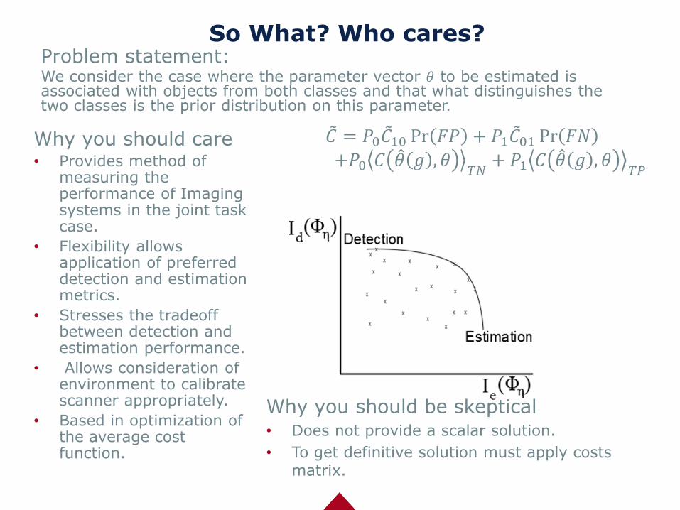
Problem statement:We consider the case where the parameter vector 𝜃 to be estimated is associated with objects from both classes and that what distinguishes the two classes is the prior distribution on this parameter.

ሚ𝐶 = 𝑃0 ሚ𝐶10 Pr 𝐹𝑃 + 𝑃1 ሚ𝐶01 Pr 𝐹𝑁

+𝑃0 𝐶 መ𝜃 𝑔 , 𝜃𝑇𝑁

+ 𝑃1 𝐶 መ𝜃 𝑔 , 𝜃𝑇𝑃

How does it work?

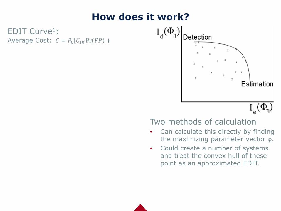
EDIT Curve1: Average Cost: 𝐶 = 𝑃0ሾ𝐶10 Pr 𝐹𝑃 +

Two methods of calculation• Can calculate this directly by finding

the maximizing parameter vector 𝜙.

• Could create a number of systems and treat the convex hull of these point as an approximated EDIT.

So What? Have you done anything with EDIT?

Stochastic Bag Example of curve generated.• Method used whereby the convex

hull of the data generated sets the EDIT curve

• Used a series of stochastically generated bags to test the performance of a fixed geometry baggage scanner.

Fixed geometry slice scans

Unique Conclusions• At low SNR Sequential scanning

outperforms multiplexed scanning.

• Spectral binning reduces estimation performance but increases detection performance at these SNR levels.

Is that all? Are you working on anything now?

We have started using real scanner systems to generate data!

What is being done:Using a fan beam CT scanner built at Duke university and scanning test bags we have been analyzing the effect of spectral systems with different angular under sampling and different reconstruction methods.

What are the potential outcomes:• Confirming or refuting simulated data

findings.

• Finding an optimal number of spectral bins.

• Finding the best reconstruction techniques for angularly under sampled scans.

Current work being headed by Sagar Mandava and Dr. Ali Bilgin with oversight from Dr. Amit Ashok.

That seemed awfully vague, how did you do your original project exactly?

The pieces that make up DHS project:

• Stochastic Bag generation

• Forward Model (Using ray trace methods)

• Detection Information (CSMI’s log w/b metric)

• Reconstruction Methods (SART,TV,Offline DL)

• Estimation Information (Normalized MSE)

• EDIT Curve calculation

• RESULTS

• Conclusion

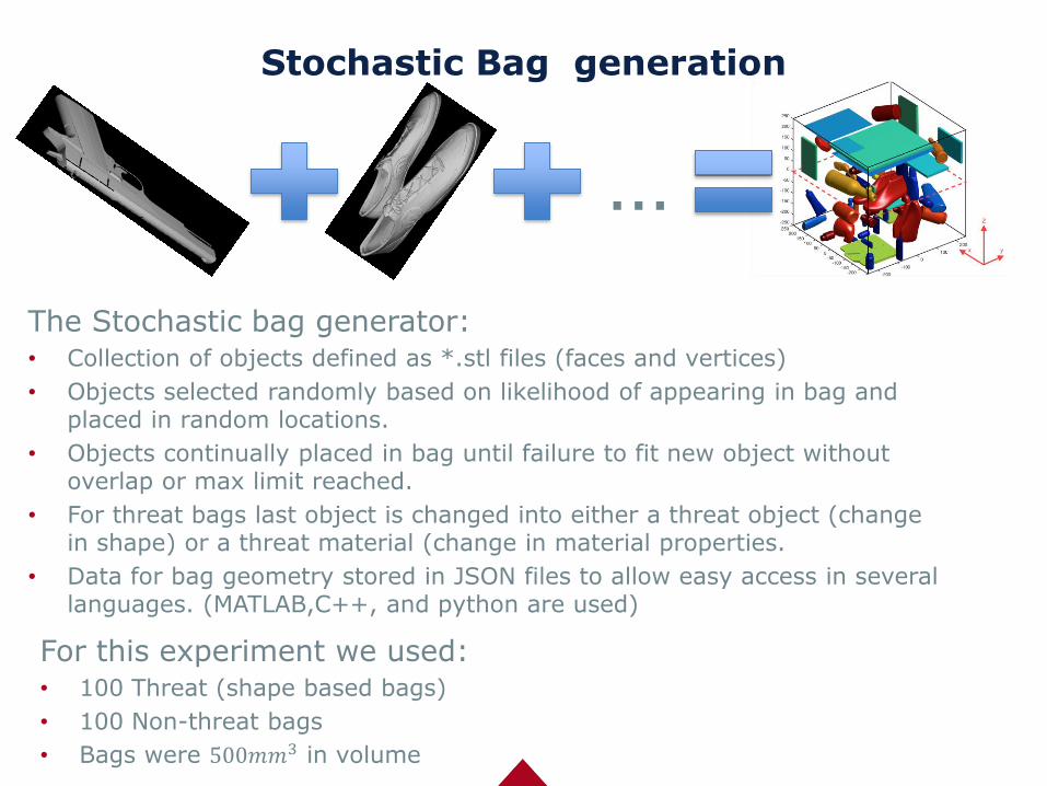
Stochastic Bag generation

The Stochastic bag generator:• Collection of objects defined as *.stl files (faces and vertices)

• Objects selected randomly based on likelihood of appearing in bag and placed in random locations.

• Objects continually placed in bag until failure to fit new object without overlap or max limit reached.

• For threat bags last object is changed into either a threat object (change in shape) or a threat material (change in material properties.

• Data for bag geometry stored in JSON files to allow easy access in several languages. (MATLAB,C++, and python are used)

For this experiment we used:• 100 Threat (shape based bags)

• 100 Non-threat bags

• Bags were 500𝑚𝑚3 in volume

…

That seemed awfully vague, how did you do your original project exactly?

The pieces that make up DHS project:

• Stochastic Bag generation

• Forward Model (Using ray trace methods)

• Detection Information (CSMI’s log w/b metric)

• Reconstruction Methods (SART,TV,Offline DL)

• Estimation Information (Normalized MSE)

• EDIT Curve calculation

• RESULTS

• Conclusion

How do you run your virtual bags through your virtual machine?

• The ray trace based method defined source location and cavity geometry. The source strength and scan time was then used to generate a number of rays in random direction within the source emission output angle.

• A GPU based algorithm then propagated each ray from its source to the first object of contact. At this point scattering and absorption effects could be calculated

• Once a path from source to detector was traced the total absorption effects of materials along the path were then used to adjust source ray strength.

That seemed awfully vague, how did you do your original project exactly?

The pieces that make up DHS project:

• Stochastic Bag generation

• Forward Model (Using ray trace methods)

• Detection Information (CSMI’s log w/b metric)

• Reconstruction Methods (SART,TV,Offline DL)

• Estimation Information (Normalized MSE)

• EDIT Curve calculation

• RESULTS

• Conclusion

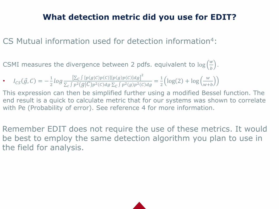
What detection metric did you use for EDIT?

CS Mutual information used for detection information4:

CSMI measures the divergence between 2 pdfs. equivalent to log𝑤

𝑏.

• 𝐼𝐶𝑆 Ԧ𝑔, 𝐶 = −1

2𝑙𝑜𝑔

σ𝐶 ∫ 𝑝 𝑔|𝐶 𝑝 𝐶 𝑝 𝑔 𝑝 𝐶 𝑑𝑔2

σ𝑐 ∫ 𝑝2 𝑔 𝐶 𝑝2 𝐶 𝑑𝑔⋅σ𝐶 ∫ 𝑝

2 𝑔 𝑝2 𝐶 𝑑𝑔=

1

2log 2 + log

𝑤

𝑤+𝑏

This expression can then be simplified further using a modified Bessel function. The end result is a quick to calculate metric that for our systems was shown to correlate with Pe (Probability of error). See reference 4 for more information.

Remember EDIT does not require the use of these metrics. It would be best to employ the same detection algorithm you plan to use in the field for analysis.

That seemed awfully vague, how did you do your original project exactly?

The pieces that make up DHS project:

• Stochastic Bag generation

• Forward Model (Using ray trace methods)

• Detection Information (CSMI’s log w/b metric)

• Reconstruction Methods (SART,TV,Offline DL)

• Estimation Information (Normalized MSE)

• EDIT Curve calculation

• RESULTS

• Conclusion

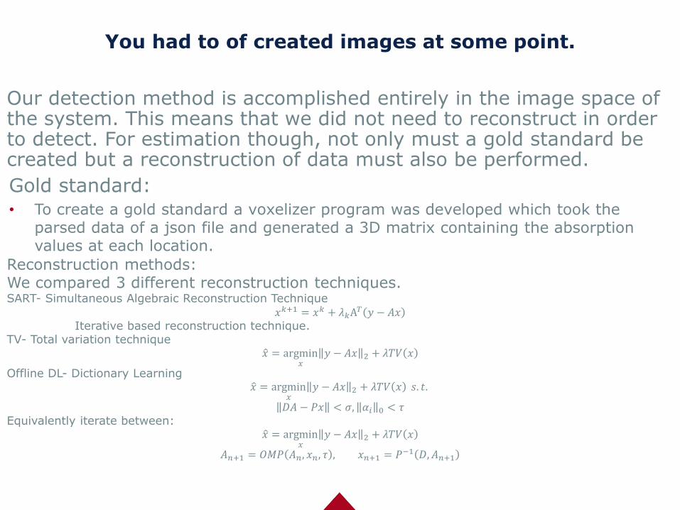
You had to of created images at some point.

Our detection method is accomplished entirely in the image space of the system. This means that we did not need to reconstruct in order to detect. For estimation though, not only must a gold standard be created but a reconstruction of data must also be performed.

Gold standard:• To create a gold standard a voxelizer program was developed which took the

parsed data of a json file and generated a 3D matrix containing the absorption values at each location.

Reconstruction methods:We compared 3 different reconstruction techniques.SART- Simultaneous Algebraic Reconstruction Technique

𝑥𝑘+1 = 𝑥𝑘 + 𝜆𝑘A𝑇 𝑦 − 𝐴𝑥

Iterative based reconstruction technique.TV- Total variation technique

ො𝑥 = argmin𝑥

𝑦 − 𝐴𝑥 2 + 𝜆𝑇𝑉 𝑥

Offline DL- Dictionary Learningො𝑥 = argmin

𝑥𝑦 − 𝐴𝑥 2 + 𝜆𝑇𝑉 𝑥 𝑠. 𝑡.

𝐷𝐴 − 𝑃𝑥 < 𝜎, 𝛼𝑖 0 < 𝜏Equivalently iterate between:

ො𝑥 = argmin𝑥

𝑦 − 𝐴𝑥 2 + 𝜆𝑇𝑉 𝑥

𝐴𝑛+1 = 𝑂𝑀𝑃 𝐴𝑛, 𝑥𝑛, 𝜏 , 𝑥𝑛+1 = 𝑃−1 𝐷, 𝐴𝑛+1

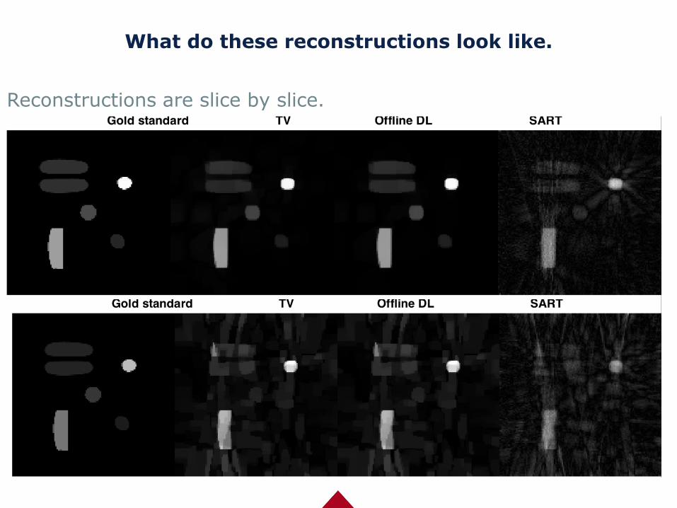
What do these reconstructions look like.

Reconstructions are slice by slice.

That seemed awfully vague, how did you do your original project exactly?

The pieces that make up DHS project:

• Stochastic Bag generation

• Forward Model (Using ray trace methods)

• Detection Information (CSMI’s log w/b metric)

• Reconstruction Methods (SART,TV,Offline DL)

• Estimation Information (Normalized MSE)

• EDIT Curve calculation

• RESULTS

• Conclusion

NMSE

• Normalized mean square error. Allows for unitless MSE we can then take the log of to compare with our detection metric.

𝑁𝑀𝑆𝐸 =1

𝑁

𝑖

𝑃𝑖 −𝑀𝑖2

ത𝑃 ഥ𝑀

That seemed awfully vague, how did you do your original project exactly?

The pieces that make up DHS project:

• Stochastic Bag generation

• Forward Model (Using ray trace methods)

• Detection Information (CSMI’s log w/b metric)

• Reconstruction Methods (SART,TV,Offline DL)

• Estimation Information (Normalized MSE)

• EDIT Curve calculation

• RESULTS

• Conclusion

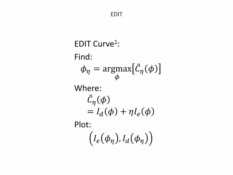
EDIT

EDIT Curve1:

Find:

𝜙𝜂 = argmax𝜙

ሚ𝐶𝜂 𝜙

Where:ሚ𝐶𝜂 𝜙

= 𝐼𝑑 𝜙 + 𝜂𝐼𝑒 𝜙

Plot:

𝐼𝑒 𝜙𝜂 , 𝐼𝑑 𝜙𝜂

EDIT

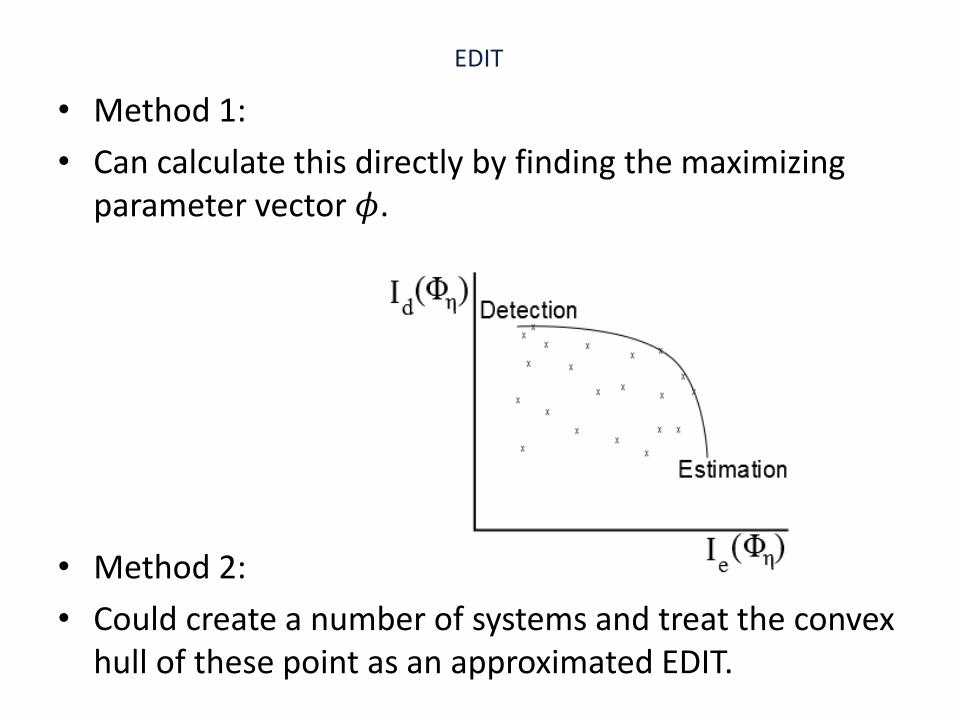
• Method 1:

• Can calculate this directly by finding the maximizing parameter vector 𝜙.

• Method 2:

• Could create a number of systems and treat the convex hull of these point as an approximated EDIT.

That seemed awfully vague, how did you do your original project exactly?

The pieces that make up DHS project:

• Stochastic Bag generation

• Forward Model (Using ray trace methods)

• Detection Information (CSMI’s log w/b metric)

• Reconstruction Methods (SART,TV,Offline DL)

• Estimation Information (Normalized MSE)

• EDIT Curve calculation

• RESULTS

• Conclusion

Stochastic Bag

Stochastic bag generator[1] used to create randomly filled 3D luggage objects2.

100 threat bags

100 non-threat bags

500𝑚𝑚3 bag volume

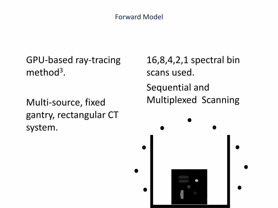
Forward Model

GPU-based ray-tracing method3.

Multi-source, fixed gantry, rectangular CT system.

16,8,4,2,1 spectral bin scans used.

Sequential and Multiplexed Scanning

EDIT Curves

Low SNR Region

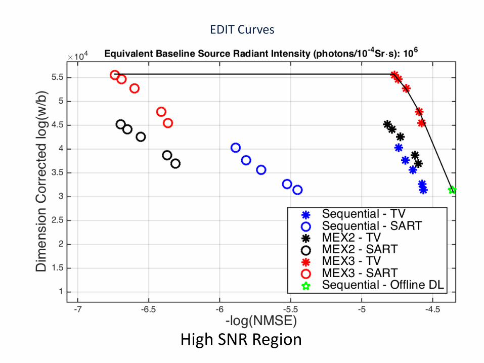
EDIT Curves

High SNR Region

Conclusion

• EDIT curves can be used to make design decisions.

• At low SNR Sequential scanning outperforms multiplexed scanning.

• Spectral binning reduces estimation performance but increases detection performance at these SNR levels.

Future Work

• Offline DL provides the best estimation but is computational intensive compared to simpler methods.

• Adjust EDIT curve to consider operator performance with estimation information.

• Use EDIT to determine the best tunable system parameters.

• Spectral binning reduces estimation performance but increases detection performance at these SNR levels.

Acknowledgments

National Institute of Health

Department of Homeland Security

University of Arizona TRIF scholarship

SMART Scholarship

SPAWAR SSC Pacific

References

[1] E. Clarkson, “Figures of merit for optimizing imaging systems on joint estimation/detection tasks,” in ADIX,9847-27 (2016).

[2] D. Coccarelli, e.a., “Information-theoretic analysis of x-ray scatter and phase architectures for anomaly detection,” in ADIX,9847-10 (2016).

[3] Q. Gong, e.a., “Rapid GPU-based simulation of x-ray transmission, scatter, and phase measurements for threat detection systems,” in ADIX,9847-25 (2016).

[4] Y. Lin, e.a., “Information-theoretic analysis of x-ray photo absorption based threat detection system for check point,” in ADIX,9847-14 (2016).

[5]A.H. Andersen, and A.C. Kak, ”Simultaneous algebraic reconstruction technique (sart): a superior implementation of the art algorithm,” Ultrasonic imaging 6.1, 81-94 (1984).

[6] Rudin, L.I., S. O. and Fatemi., E., “Nonlinear total variation based noise removal algorithms," Physica D:Nonlinear Phenomena 60.1, 259-268 (1992).

[7] Aharon, Michal, M. E. and Bruckstein, A., “K-svd: An algorithm for designing over complete dictionaries for sparse representation," Signal Processing, IEEE Transactions on 54.11, 4311-4322 (2006).

How do we define the estimate for joint tasks?

We consider the case where the parameter vector 𝜃 to be estimated is associated with objects from both classes and that what distinguishes the two classes is the prior distribution on this parameter.Basis Equations:

Cost Matrix: 𝐶00 𝐶01𝐶10 𝐶11

Probabilities Matrix: Pr 𝑇𝑁 Pr 𝐹𝑁Pr 𝐹𝑃 Pr 𝑇𝑃

Average Cost: 𝐶 = 𝑃0 𝐶10 Pr 𝐹𝑃 + 𝐶00 Pr 𝑇𝑁

+𝑃1 𝐶01 Pr 𝐹𝑁 + 𝐶11 Pr 𝑇𝑃 + 𝑃1 𝐶 𝜃 𝑔 , 𝜃

Differential cost: ሚ𝐶10 = 𝐶10 − 𝐶00; ሚ𝐶01 = 𝐶01 − 𝐶11𝐵 = 𝑃0𝐶00 + 𝑃1𝐶11

New costs equation to Minimize:ሚ𝐶 = 𝑃0 ሚ𝐶10 Pr 𝐹𝑃 + 𝑃1 ሚ𝐶01 Pr 𝐹𝑁 + 𝑃0 𝐶 𝜃 𝑔 , 𝜃

𝑇𝑁+ 𝑃1 𝐶 𝜃 𝑔 , 𝜃

𝑇𝑃