estimation and correction of systematic … 2017/16...estimation and correction of systematic model...

ESTIMATION AND CORRECTIONOF SYSTEMATIC MODEL

ERRORS IN GFS

Acknowledgements: Dr. James Car ton Dr. Fangl in Yang (NCEP) , Dr. J im Jung , Dr. Mark I rede l l , and Dr. Dary l Kle i s t

NGGPS PI MeetingAugust 2, 2017

Kriti Bhargava (student), Eugenia Kalnay, Jim Carton

Goals

(i) Estimate the model deficiencies in the GFS that lead to systematic forecast errors

(ii) Implement an online correction (i.e., within the model) scheme to correct GFS

following the methodology of Danforth and Kalnay, 2008.

(iii) Provide guidance to optimize design of subgrid-scale physical parameterizations.

The empirical correction scheme can then be replaced by these.

8/2/2017 EUGENIA KALNAY NGGPS PI MEET 2017 2

MotivationSYSTEMATIC FORECAST ERROR IN GFS

SYSTEMATIC MODEL ERRORS


Forecast ErrorsNumerical weather prediction models are limited by errors in model forecast resulting from

• Model bias• Inaccuracies in initial condition


Forecast MSE

Systematic c𝐨𝐨𝐨𝐨𝐨𝐨𝐨𝐨𝐨𝐨𝐨𝐨𝐨𝐨𝐨𝐨(𝒙𝒙𝒇𝒇 − �𝒙𝒙𝒕𝒕)𝟐𝟐

Model Bias

Observation bias

Random component(𝒙𝒙𝒇𝒇′ − 𝒙𝒙𝒕𝒕′)𝟐𝟐

Analysis Errors

Chaotic growth

Initially small, but as the model is integrated in time the errors grow and interact nonlinearly with systematic and random errors until the model loses all forecast skill.

Systematic Forecast Errors in GFS• Systematic forecast errors are a significant portion of the total forecast error in weather prediction

models, such as the Global Forecast System (GFS).


Figure 1. Zonal mean RMS systematic error (left) and total error (right) in temperature after 16 days. The range of temperature systematic errors is ~1/3 of total temperature error range after 2 weeks. (Courtesy of Dr. Glenn White).

Characterizing model error (after Danforth and Kalnay, 2008)


𝑥𝑥𝑚𝑚𝑒𝑒 = 𝑏𝑏 + ∑𝑙𝑙=1𝐿𝐿 𝛽𝛽𝑙𝑙(𝑡𝑡)𝑒𝑒𝑙𝑙 + ∑𝑛𝑛=1𝑁𝑁 𝛾𝛾𝑛𝑛(𝑡𝑡)𝑓𝑓𝑛𝑛 + 𝑥𝑥𝑚𝑚𝑟𝑟𝑟𝑟𝑛𝑛𝑟𝑟

Constant term: Time mean

Periodic errors described using leading EOFs

State-dependent model error given by the leading SVD modes fn of the covariance of

the coupled model state anomalies and corresponding error anomalies

Random Error

Our goal is to estimate the three components of the systematic error

Past StudiesCORRECTION SCHEMES


Correction Schemes

OFFLINE CORRECTION SCHEME

• Apply a statistical correction for each forecast length after the forecast is completed

• Allow forecast errors to grow until the end of the forecast cycle

• Physical origin obscured as errors grow non-linearly after short time

ONLINE CORRECTION SCHEME

• Estimate and correct the bias during the model integration

• Continuously corrected forecasts at all lead times

• Reduces non linear error growth of bias

• Large forcing might disturb physical balance of model variables


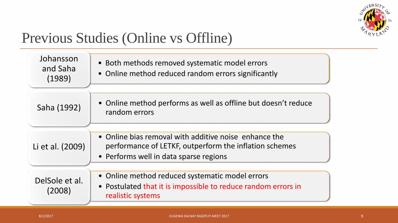
Previous Studies (Online vs Offline)


• Both methods removed systematic model errors• Online method reduced random errors significantly

Johansson and Saha

(1989)

• Online method performs as well as offline but doesn’t reduce random errorsSaha (1992)

• Online bias removal with additive noise enhance the performance of LETKF, outperform the inflation schemes

• Performs well in data sparse regionsLi et al. (2009)

• Online method reduced systematic model errors• Postulated that it is impossible to reduce random errors in

realistic systems

DelSole et al. (2008)

Previous studies … (Danforth & Kalnay 2007, 2008ab)Methods Used

• Time averaged analysis correction: the average correction that the observations make on the 6hr forecast

�̇�𝑥 𝑡𝑡 = 𝑀𝑀 𝑥𝑥 𝑡𝑡 +𝛿𝛿𝑥𝑥6𝑟𝑟𝑎𝑎

6 ℎ𝑟𝑟• Periodic component correction (diurnal correction): linearly interpolated leading EOFs (low dimension

approach)• State dependent correction: introduced new method using SVD of coupled analysis correction and

forecast state anomalies (low dimension approach)Results

• Online correction performance was slightly better than the operational statistical method applied a posteriori

• Correcting bias also reduced random errors


Presenter

Presentation Notes

reduced

Proposed Method for GFSESTIMATE MODEL DEFICIENCIES IN GFS WITH AN. INCREMENTS

CORRECT GFS ONLINE FOR MODEL DEFICIENCIES


Estimation of model deficiencies• Model biases are estimated from the time average of the 6-hr analysis increments (AIs)

• AIs are the difference between the gridded analysis and forecast: the corrections that the observations make on the 6-hr forecasts

𝜹𝜹𝒙𝒙𝒂𝒂𝒂𝒂𝟔𝟔 = 𝒙𝒙𝒂𝒂𝟔𝟔 − 𝒙𝒙𝒇𝒇𝟔𝟔

Time mean

• Estimate seasonal model bias as the seasonal average (DJF, MAM, JJA, and SON) of the AIs for surface pressure, temperature, winds and specific humidity during the five years 2012-2016

Periodic Component: periodic AIs at sub-monthly scales

• First calculate the anomalies of the 6-hourly AIs with respect to their monthly averages

• Decompose these anomalies into a complete set of 120 Empirical Orthogonal Functions (EOFs) and corresponding principal component time series


Correcting GFS online for model deficiencies• Plan to follow the methods comprehensively developed by Danforth and Kalnay [DKM07; Danforth and

Kalnay, 2008(GRL) and Danforth and Kalnay, 2008(JAS)]

�̇�𝒙 𝒕𝒕 = 𝐌𝐌 𝐱𝐱 𝒕𝒕 + 𝛅𝛅𝒙𝒙𝒂𝒂𝒂𝒂𝟔𝟔

𝟔𝟔−𝒉𝒉𝒉𝒉

• Correcting diurnal and semi-diurnal bias using low dimensional estimate

�𝒍𝒍=𝟏𝟏

𝑵𝑵

𝜷𝜷𝒍𝒍(𝒕𝒕)𝒆𝒆𝒍𝒍

• 𝑒𝑒𝑙𝑙 : leading EOFs from the anomalous error field (time independent term)

• 𝛽𝛽𝑙𝑙 : time dependent amplitude, estimated by averaging over the daily cycle in the training period

• N : number of leading EOFs


Preliminary ResultsSEASONAL BIAS ESTIMATION

PERIODIC BIAS ESTIMATION


Seasonal Bias Estimation

8/2/2017EUGENIA KALNAY NGGPS PI MEET 2017 15

• Significant biases that are geographically anchored with continental scales in the GFS.

• Despite major changes made to the data assimilation scheme in May 2012, the bias corrections retain their major features throughout 2012 to 2014

JJA mean 6-hr Analysis Increment at ~850mb

Presenter

Presentation Notes

Added a few corrections (biases)


Change in surface air temperature mean bias, June 2014 (a) - June 2015(b) and the difference in RTG and OI SST (c).

JJA mean 6-hr Analysis Increment at ~850mb

Seasonal Bias Estimation …

• Amplitude of the bias declines in 2015, especially over the ocean

• In north, the reduction might be due to change in the SST boundary condition

• In south, the reduction in bias is due to updating of the Community Radiative Transfer Model and improvements in radiance assimilation

• Bias represented by AIs over oceans in 2012-2014 also arise from bias in prescribed SSTs


JJA 2014 mean 6-hr AI at ~ 850 mb

Periodic Bias Estimation

• Large diurnal component moves westward following the motion of the Sun. Also a significant semi-diurnal signal

• Amplitude comparable to the seasonal bias, thus making correction of diurnal and semi-diurnal bias is also critical

Presenter

Presentation Notes

moves, is

Periodic Bias Estimation: EOF Analysis s Estimation


Periodic Bias Estimation: EOF Analysis s Estimation


The errors in diurnal cycle represented with the first four modes are almost indistinguishable when compared with all (120) modes

Proposed Future WorkWORK PLAN

TIMELINE FOR COMPLETION OF DISSERTATION AND PUBLICATIONS


Work Plan• Results for bias estimation in GFS support the application of the approaches used by DKM07.

• Two challenges that now arise when using them for online correction :

1. Accounting for contributions of observation biases to the AIs.

• AIs should be adjusted for observation biases before using them to correct the model bias.

• Erroneously correcting the model for an observation bias should result in an increase of the AI’s, this should help differentiate model and observation bias

2. How to utilize the past estimates to correct present models?

• Plan to use the successful approach of Greybush et al. [2012], who used the rolling mean of a limited number of past AIs (e.g., the past 21 days) to correct the model online.


Presenter

Presentation Notes

21

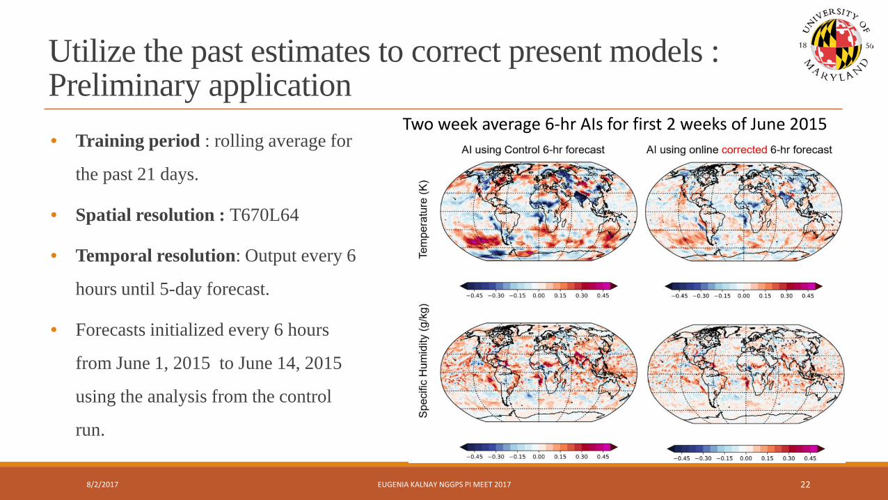
Utilize the past estimates to correct present models : Preliminary application• Training period : rolling average for

the past 21 days.

• Spatial resolution : T670L64

• Temporal resolution: Output every 6

hours until 5-day forecast.

• Forecasts initialized every 6 hours

from June 1, 2015 to June 14, 2015

using the analysis from the control

run.


Two week average 6-hr AIs for first 2 weeks of June 2015

Work Plan


Apply Online Correction◦Apply the same corrections to the winds and surface pressure◦Correct periodic bias (diurnal and semidiurnal errors)

After Online Correction◦Compare forecast bias improvement with statistical bias correction made a

posteriori.◦Check whether reducing the mean and periodic bias also reduces forecast random

errors during their nonlinear growth.◦Apply this method to FV3 to provide simple verification tool to optimizing

physical parameterizations◦Work with EMC scientists on using the Analysis Increments as an efficient tool to

facilitate testing impacts of new parameterizations on FV3.

Work Plan


Apply Online Correction◦Apply the same corrections to the winds and surface pressure◦Correct periodic bias (diurnal and semidiurnal errors)

After Online Correction◦Compare forecast bias improvement with statistical bias correction made a

posteriori.◦Check whether reducing the mean and periodic bias also reduces forecast random

errors during their nonlinear growth.◦Apply this method to FV3 to provide simple verification tool to optimizing

physical parameterizations◦Work with EMC scientists on using the Analysis Increments as an efficient tool to

facilitate testing impacts of new parameterizations on FV3.Thank You

estimation and correction of systematic … 2017/16...estimation and correction of systematic model...

Documents