estimating water storage capacities in soil at catchment scales

ESTIMATING WATER STORAGE CAPACITIES IN SOILAT CATCHMENT SCALES

TECHNICAL REPORTReport 03/3May 2003

Neil McKenzie / John Gallant / Linda Gregory

C O O P E R A T I V E R E S E A R C H C E N T R E F O R C A T C H M E N T H Y D R O L O G Y

McKenzie, Neil J. (Neil James), 1958- ...

Estimating Water Storage Capacities in Soil atCatchment Scales

Bibliography.

ISBN 1 876006 97 8.

1. Watersheds. 2. Water-storage. 3. Soil moisture - Measurement. 4. Soilporosity. I. Gallant, John, 1958- ... II. Gregory, Linda, 1969- . III.Cooperative Research Centre for Catchment Hydrology. IV. Title. (Series :Report (Cooperative Research Centre for Catchment Hydrology); 03/3).

628.13

Keywords

Soil/Water SystemsStorageWater-Soil-Plant InteractionsSoil DataModellingSurveyMaps and MappingLand ResourcesSoil (Types of)Soil (Characteristics of)

© Cooperative Research Centre for Catchment Hydrology, 2003

COOPERATIVE RESEARCH CENTRE FOR CATCHMENT HYDROLOGY

i

Estimating Water Storage Capacities in Soil at Catchment Scales

Neil McKenzie, John Gallant and Linda Gregory

Technical Report 03/3May 2003

Preface

The Cooperative Research Centre (CRC) for Catchment Hydrology aims to provide land and water managers with the tools and skills to make informed decisions on whole catchments. The development of integrated modelling systems is a central activity. The capacity of models to provide reliable predictions of catchment behaviour is increasingly being constrained by the quality of input data. Soil and landscape attributes can affect water and pollutant balances but appropriate data, even for synoptic modelling, have not been readily available across large parts of Australia. This report addresses one instance of this constraint – the estimation of water storage capacities in soils at catchment scales. It demonstrates how careful integration of digital terrain and conventional land resource data can benefit catchment hydrology – the promising results bode well for the CRC’s modelling and prediction studies.

This report describes some of the work conducted by the CRC’s program concerning land-use impacts on rivers. The program is focused upon the impact of human activities upon the land and stream environment and the physical attributes of rivers. We are concerned about managing impacts for catchments ranging in size from a single hillslope to several thousands of square kilometres. The specific impacts we are considering are changes in streamflow, changes to in-stream habitat by the movement of coarse sediment, and changes to water quality (sediment, nutrients and salt). If you wish to find out more about the program’s research I invite you to first visit our website at at http://www.catchment.crc.org.au/programs/projects/index.html.

Peter HairsineCSIRO Land and Water Program Leader, Land-Use Impacts on RiversCRC for Catchment Hydrology


ii

Acknowledgements

Andrew Western helped us at various times and provided useful comments on an earlier draft. Peter Hairsine and Lu Zhang are also thanked for their assistance.


iii

Summary

Landscapes vary in their capacity to store water. Estimates of water storage capacities in soil are required to allow a better analysis of interactions between vegetation and stream flow from local to regional scales. This is particularly relevant to simulation studies relating to dryland salinity, farm forestry and water security. This report investigates how land resource data can be used to improve estimates of water storage capacities in soil at catchment scales.

A distinction is made between total water storage, profile available water capacity, and plant available water capacity. The latter requires a consideration of plant root distribution. A requirement for each variable is reliable estimation of soil depth. A scheme for estimating soil depth is proposed. It uses new methods of terrain analysis, in conjunction with conventional sources of soil information, to provide spatially explicit predictions of soil depth. Published pedotransfer functions or water retention measurements are then used to estimate profile available water capacity. A simple model for estimating root distributions is proposed. The single-parameter model produces a profile-scaling factor and this is used with the profile available water capacity to calculate the plant available water capacity. Different scaling factors can be used for perennial vegetation, annual crops or pastures. The methods are evaluated using data for the Kyeamba Creek catchment, south-east of Wagga Wagga, New South Wales. The methods can be readily applied across much larger areas.

We briefly examine the relative gains in predictive success from higher resolution sets of data for soil and landform. The performance of the Digital Atlas of Australian Soils, used in conjunction with the continental 9″ digital elevation model (DEM), is compared with a higher resolution DEM (25 m grid cells) and 1:100 000 scale soil survey data.

The scheme for estimating water storage capacities in soil at catchment scales provides more realistic predictions than previously available from land resource survey data. The innovative method of terrain analysis appears to be robust and initial results are promising. Comprehensive field-testing is required. Further lines of work are proposed.


iv


v

Preface i

Acknowledgements ii

Summary iii

List of Tables vi

List of Figures vii

1. Introduction 11.1 Defining Water Storage 1

1.2 Current Methods for Prediction Using Land Resource Survey Data 2

1.2.1 Continental Extent 2

1.2.2 Regional Extent 3

2. Estimating Profile Available Water Capacity 72.1 Options 7

2.2 Estimating Profile and Layer Thickness 7

2.2.1 Total Profile Depth 7

2.2.2 A Horizon Thickness 10

2.3 Water Retention 11

3. Estimating Plant Available Water Capacity 133.1 Scaling Function to Reflect Root Density 13

3.2 Validation Data 14

4. Results and Discussion 17

5. Directions 25

6. References 27


vi

List of Tables

Table 1 Data derived from Chen and McKane (1996). The water retention estimates are both depth-weighted and area-weighted averages. The scaling parameter (Xi) is an area-weighted average 12

Table 2 Suggested values of Xi for a select number of soil types (after Isbell 1996). Interpretations based largely on data provided by Williams (1983) 15

Table 3 Mean profile depth and available water capacity for Kyeamba Catchment using two estimation procedures 17


vii

List of Figures

Figure 1 Pore space relations for a soil profile 1

Figure 2 Predicted profile depth using only the Atlas of Australian Soils (McKenzie et al. 2000) for the Kyeamba Catchment 4

Figure 3 Predicted profile available water capacity using only the Atlas of Australian Soils (McKenzie et al. 2000) for the Kyeamba Catchment 5

Figure 4 The relationship between soil depth and the topographic wetness index (TWI) 8

Figure 5 Explicit weighting functions for transitional zones 9

Figure 6 Patterns of soil depth on (a) slopes where sediment movement is limited by transport and (b) slopes where sediment movement is limited by supply 10

Figure 7 Scaling relations for converting profile available water capacity to plant available water capacity 13

Figure 8 Total plant available water store for the profile (assuming a total soil depth of 5 m) as a function of average profile available water capacity (mm/m) and the root-density scaling parameter, Xi 14

Figure 9 Predicted soil depth using the 9″ DEM and Atlas of Australian Soils for the Kyeamba Catchment 18

Figure 10 Predicted soil depth using the 25 m DEM and 1:100 000 soil landscape mapping for the Kyeamba Catchment 19

Figure 11 Predicted profile available water capacity using the 9″ DEM and Atlas of Australian Soils for the Kyeamba Catchment 20

Figure 12 Predicted profile available water capacity using the 25 m DEM and 1:100 000 soil landscape mapping for Kyeamba Catchment 21

Figure 13 Predicted and measured soil depths for the Griggward Study Area (Gessler 1996) using different terrain and soil map data sources 22

Figure 14 Predicted and measured soil depths for the Ladysmith Study Area (Gessler 1996) using different terrain and soil map data sources 22

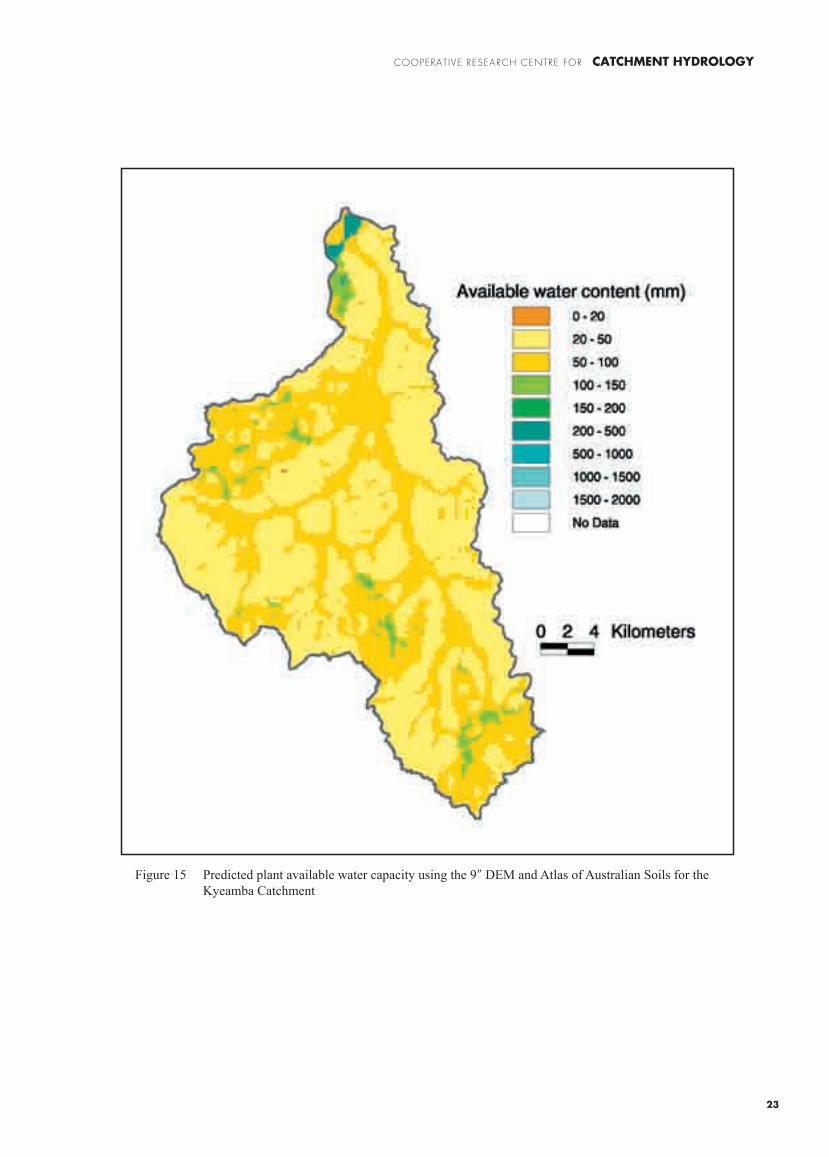
Figure 15 Predicted plant available water capacity using the 9″ DEM and Atlas of Australian Soils for the Kyeamba Catchment 23

Figure 16 Predicted plant available water capacity using the 25 m DEM and 1:100 000 soil landscape mapping for Kyeamba Catchment 24


viii


1

1. Introduction

Simulation models for predicting the impact of vegetation on stream flow have the potential to be improved through more realistic depiction of water storage in landscapes. Estimates of water storage – preferably with a mean and variance – have to be provided in the first instance at the scale of the small catchment. However, estimates are also required for small to medium-sized catchments (perhaps up to 500 km2) to thoroughly explore scenarios for vegetation change.

The potential for estimating water storage capacities in soil using both digital elevation models and data from soil and land resource surveys has been recognized for some time. However, appropriate methods of analysis and interpretation have been lacking. This

report proposes a method for estimating the water storage capacity of the upper 5 m of the landscape. A new procedure is proposed that uses a combination of quantitative terrain analysis and conventional land resource information. The method is applied to the Kyeamba Creek catchment in southern New South Wales. This is a sub-catchment of the Murrumbidgee, the latter being a focus catchment for the CRC for Catchment Hydrology.

1.1 Defining Water Storage

Water storage will be considered using conventional concepts of soil physics (see Figure 1).

Total water storage is defined as the equivalent depth of water within a specified depth of soil when the profile is at a notional field capacity (i.e., matric potential of –10 kPa).

Figure 1 Pore space relations for a soil profile. The total water storage is the volume occupied by unavailable and available water. The plant available water capacity is less than the profile water available capacity because of limitations to root growth and function


2

Profile available water capacity is defined as the equivalent depth of water within a specified depth of soil between the notional field capacity and wilting point (i.e., matric potentials of –10 kPa and –1.5 MPa respectively) – in other words, the difference in volumetric water content between these potentials, integrated over the depth of the profile.

Plant available water capacity is defined as the equivalent depth of water, within a specified depth of soil, between the upper and lower limit of water extraction by a nominated plant species or vegetation structural form. Plant available water capacity will nearly always be significantly less than profile available water capacity due to soil constraints to root growth. For example, these may be physical limitations (excessive strength or poor aeration), nutrient limitations (deficiencies due to low absolute levels of essential nutrients or restricted availability due to pH), toxicities (e.g., salinity, boron, aluminium, sodium) or pathogens (e.g., root diseases). Plant physiological factors will also play a role (e.g., root system morphology).

Estimation of total water storage and profile available water capacity requires knowledge of soil physical properties only, while plant available water capacity involves consideration of a wide range of soil and plant characteristics.

While the above definitions have many limitations for both the prediction of plant growth and runoff (see Hillel 1998), they will suffice as a first approximation for the purpose of this report.

1.2 Current Methods for Prediction Using Land Resource Survey Data

1.2.1 Continental Extent

Estimates of soil hydraulic properties, including storage, have been generated for the continent using digital versions of the Atlas of Australian Soils (Northcote et al. 1968, McKenzie and Hook 1992, McKenzie et al. 2000). The source data and accompanying interpretation tables have many limitations. McKenzie et al. (2000) consider the most significant to be:

• Reconnaissance scale soil-landscape maps usually have a low predictive capability for individual soil properties (Beckett and Webster 1971; Wilding

and Drees 1983). This predictive capability is further diminished by the uncertainty associated with each interpretation of the original map.

• The quality of the Atlas mapping varies substantially between regions in Australia.

• The Atlas of Australian Soils does not provide information on the area within each polygon occupied by the component soil type. As a result, area-weighted averages cannot be calculated. While a dominant soil type can be specified for each unit, it may occupy a very limited area within a given unit (perhaps 20%). Any analysis based on an interpretation of the dominant soil is therefore of restricted value. An alternative is to calculate average values for the most common soils. However, an average value can also be misleading when, in reality, there is a clear dominant soil and the minor soils have sharply contrasting properties.

• Very large variation within each map unit is normal. Some units have up to 20 soils listed. It is common for the within-unit variation to be as great as the between-unit variation. This is an inescapable problem with reconnaissance scale soil-landscape mapping.

• Some soil types are far more variable with respect to the interpreted properties than others.

• Many landscape processes (e.g., erosion, salinization) do not correlate in a simple way with the Atlas units because the description of soils is based on profile morphology. Profile morphology may have a poor or complex relationship with soil physical and chemical properties, and through these, with landscape processes.

• The spatial arrangement of soils within a landscape may have an overriding impact on landscape processes. The Digital Atlas and its associated tables provide limited information on spatial arrangement.

• Predictions of soil depth have an overriding control on the estimate of soil water storage and it is known that depth estimates are the least reliable.

Despite these daunting limitations, the Digital Atlas of Australian Soils, in conjunction with the interpretations of McKenzie and Hook (1992) and McKenzie et al.


3

(2000), have been useful for a range of applications including synoptic scale modelling of water balance, nutrient cycling, crop yield, biomass production, risk of groundwater contamination and runoff (e.g., NLWRA 2001, Ladson et al. 2002). However, an initial assessment of the utility of the predictions for water storage and catchment modelling indicated that they only marginally improved the prediction of runoff (Zhang pers. com.).

Figures 2 and 3 show estimates of soil depth and profile available water capacity from the Digital Atlas for the Kyeamba Catchment, south-east of Wagga Wagga, New South Wales. The National Land and Water Resources Audit (2001) produced new continental-level predictions for large parts of Australia that supersede the Digital Atlas. These predictions are paving the way for an improved nation-wide coverage, but thorough testing is yet to be completed although many of the problems listed above remain.

1.2.2 Regional Extent

Medium-scale land resource maps are available for an increasing area across Australia. The more recent maps (e.g. Chen and McKane 1996, Jenkins 2000) often have a cartographic scale of 1:100 000. It is unlikely for more detailed survey data to become available for large regions in south-east Australia during the next decade. Many of the problems inherent in the older continental-scale maps also apply to these medium scale maps, albeit to a lesser degree. A particular problem for most forms of land resource survey is the unreliable estimation of soil depth. There are several issues.

Most soil profile data used to construct soil maps come from soil pits, auger borings or mechanical drilling. Current databases are deficient because the lower depth of sampling has been constrained either by:

• convention (e.g., only the solum is described (i.e., A and B horizons))

• survey purpose (e.g., agriculturally focused surveys emphasize soil variation in the first metre or so)

• physical limitations (e.g., gravel layers or duricrusts prevent coring to depth)

• equipment limitations (e.g., hand-operated augers are rarely used to make routine observations deeper than 2 m).

Current databases have minimal information on the occurrence of layers limiting root growth. This is a difficult technical task because species have varying capacities to penetrate hostile environments that are characterized by large soil strength, low levels of nutrients, and restricted aeration. Predicting root limitations for perennials is particularly difficult. Many have developed symbiotic relationships with mycorrhiza, and presence of these organisms can result in plentiful root growth and water extraction in situations where standard soil test results indicate severe nutrient deficiency. Our capacity to predict the distribution and function of soil microorganisms is very poor.

Another weakness of conventional land resource maps is the reliance on polygons as a means for spatial prediction of soil properties (e.g., Figures 2 and 3). It is standard practice for a range of soil conditions to be ascribed to a particular polygon. This has been necessary because cartographic restrictions prevent depiction of local soil variation associated with changes in landform. As a result, a polygon description may state ‘soil depth varies from shallow on ridge crests to deep in valley bottoms’. While the spatial pattern is described, it is difficult to use in simulation modeling without some form of explicit spatial attribution.

Our contention is that estimates of soil depth, and more specifically, the depth to which plants can extract water, can be greatly improved through careful interpretation of conventional land resource surveys in conjunction with terrain analysis.

We aimed to partly remedy the limitations with existing schemes for predicting plant available water and total water storage in catchments by:

• Using new methods of terrain analysis in conjunction with conventional sources of soil information to provide better spatial prediction of soil depth

• Devising more appropriate schemes for estimating water retention properties of soil and regolith materials.


4

We were also interested in the relative gains in predictive success through the use of higher resolution data for soils and elevation. The Digital Atlas of Australian Soils and the 9˝ DEM provide a continental coverage. Such data are known to have fundamental limitations because they cannot accurately portray soil variation at the scale of the hillslope – the scale at which a large proportion of variation occurs. However, an ability to predict even coarse-level differences in water storage would be of great value for synoptic level modelling.

As noted earlier, land resource maps at a cartographic scale of 1:100 000 are becoming more readily available with comprehensive coverages in some parts of the country (e.g., agricultural lands of Western Australia, South Australia). Likewise, digital elevation models with a grid size of 25 m are also widely available. We have therefore compared predictions using such data with those available at the continental level.

Figure 2 Predicted profile depth using only the Atlas of Australian Soils (McKenzie et al. 2000) for the Kyeamba Catchment


5

Figure 3 Predicted profile available water capacity using only the Atlas of Australian Soils (McKenzie et al. 2000) for the Kyeamba Catchment


6


7

2. Estimating Profile Available Water Capacity

2.1 Options

The estimation of profile available water capacity requires information on the:

• Thickness of individual layers

• Water retention properties of each layer (as a minimum, water contents at –10kPa and –1.5MPa).

New methods for estimating the thickness of individual layers are described in the next section. There is a large literature on the estimation of water retention properties. For catchment hydrology purposes in Australia, there are several immediate options.

• Undertake direct measurements of water contents at –10 kPa and –1.5 MPa on the major soil types present within a catchment; or

• To avoid the cost of water retention measurements, estimate water contents with continuous pedotransfer functions, which use other soil properties (e.g., texture, structure, and bulk density) from each layer as explanatory variables (e.g., Williams et al. 1992)

• As a last resort, estimate water contents using look-up tables such as those presented by McKenzie et al. (2000) for taxonomic classes of soil.

The first option is not feasible in many parts of Australia because of the limited land resource survey coverage. In New South Wales, the 1:100 000 land resource survey series does include measures of the –10kPa and –1.5MPa water contents. However, there are some issues that can restrict the utility of these data. Measurements are made on sieved material and this is generally considered to be inappropriate at potentials close to zero (i.e., the –10kPa determination). Measurements of bulk density are not undertaken so the necessary conversion to a volumetric estimate of available water capacity is compromised (a default value for bulk density is assumed). Finally, published

values for determinations on soils that are either sodic, have vertic properties, or both, are sometimes implausible. Reported water contents at –10kPa for these soils are sometimes extremely large and the porosity required to store such a volume implies an extremely small bulk density that is inconsistent with the description of the material provided in the reports. However, the data in the survey reports are often the best available.

The merits of the second and third options are considered by McKenzie and Cresswell (2002) in their detailed account of estimation procedures for soil hydraulic properties using pedotransfer functions.

2.2 Estimating Profile and Layer Thickness

2.2.1 Total Profile Depth

Estimation of catchment storage depends heavily on the capacity to predict soil and regolith depth.1 This depth is controlled by several factors including the histories of:

• weathering (intensity, duration, and ease of weathering of the parent material)

• deposition (e.g., rates of aeolian accession, alluvial deposition, and colluvial deposition)

• erosion.

While a model of material balances could be constructed to enable prediction of soil depth, parameterisation is difficult, particularly in relation to processes that may have proceeded at varying rates over hundreds of thousands of years. Most processes are understood in only qualitative terms across broad areas although estimates may be possible at particular locations where good fortune allows some disentangling of causality; for example, the work by Pillans (1999) on rates of soil formation on basalts, or isotope studies and modelling by Heimsath et al. (2001). Even if rates of processes are tractable, estimating the duration of weathering, deposition, and erosion at a given site is problematic.

For these reasons, we have adopted an empirical approach where great reliance is placed on landform

1 The terms soil and regolith are used interchangeably in this report. In practice, the terms often reflect the training of the worker. Soil is used here to include all layers that show some degree of pedologic organisation (see Isbell 1996, p7).


8

to provide an estimate of material balances between erosion and deposition (although no explicit allowance is made for aeolian accession). Terrain variables are used to scale soil depths derived from land resource survey reports. The following describes the method when using a 25 m resolution digital elevation model and 1:100 000 soil-landscape map unless otherwise stated.

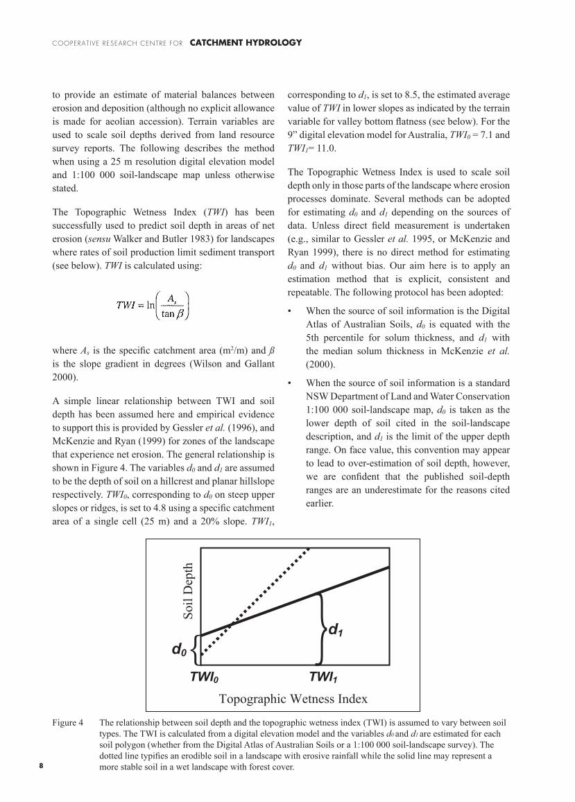
The Topographic Wetness Index (TWI) has been successfully used to predict soil depth in areas of net erosion (sensu Walker and Butler 1983) for landscapes where rates of soil production limit sediment transport (see below). TWI is calculated using:

where As is the specific catchment area (m2/m) and ß is the slope gradient in degrees (Wilson and Gallant 2000).

A simple linear relationship between TWI and soil depth has been assumed here and empirical evidence to support this is provided by Gessler et al. (1996), and McKenzie and Ryan (1999) for zones of the landscape that experience net erosion. The general relationship is shown in Figure 4. The variables d0 and d1 are assumed to be the depth of soil on a hillcrest and planar hillslope respectively. TWI0, corresponding to d0 on steep upper slopes or ridges, is set to 4.8 using a specific catchment area of a single cell (25 m) and a 20% slope. TWI1,

corresponding to d1, is set to 8.5, the estimated average value of TWI in lower slopes as indicated by the terrain variable for valley bottom flatness (see below). For the 9” digital elevation model for Australia, TWI0 = 7.1 and TWI1= 11.0.

The Topographic Wetness Index is used to scale soil depth only in those parts of the landscape where erosion processes dominate. Several methods can be adopted for estimating d0 and d1 depending on the sources of data. Unless direct field measurement is undertaken (e.g., similar to Gessler et al. 1995, or McKenzie and Ryan 1999), there is no direct method for estimating d0 and d1 without bias. Our aim here is to apply an estimation method that is explicit, consistent and repeatable. The following protocol has been adopted:

• When the source of soil information is the Digital Atlas of Australian Soils, d0 is equated with the 5th percentile for solum thickness, and d1 with the median solum thickness in McKenzie et al. (2000).

• When the source of soil information is a standard NSW Department of Land and Water Conservation 1:100 000 soil-landscape map, d0 is taken as the lower depth of soil cited in the soil-landscape description, and d1 is the limit of the upper depth range. On face value, this convention may appear to lead to over-estimation of soil depth, however, we are confident that the published soil-depth ranges are an underestimate for the reasons cited earlier.

Figure 4 The relationship between soil depth and the topographic wetness index (TWI) is assumed to vary between soil types. The TWI is calculated from a digital elevation model and the variables d0 and d1 are estimated for each soil polygon (whether from the Digital Atlas of Australian Soils or a 1:100 000 soil-landscape survey). The dotted line typifies an erodible soil in a landscape with erosive rainfall while the solid line may represent a more stable soil in a wet landscape with forest cover.

��

��

��

}{

��


9

Separate protocols will be developed for other sources of land resource information.

A limitation of existing methods for estimating soil water storage has been the inability to identify areas where deep regolith occurs. Limitations of existing land resource information have been noted already. Likewise, the use of terrain attributes such as the TWI becomes less reliable in lower parts of the landscape. The TWI uses information from the point of interest (slope) and the upslope area (the specific catchment area). However, landscape processes that determine deposition are related to a range of other factors including landform below the point of interest and the local base level of the drainage network.

Gallant and Dowling (2003) have derived a new terrain attribute, the Multi-Resolution Valley Bottom Flatness (MRVBF) index, which provides more realistic predictions of where depositional zones occur in the landscape.

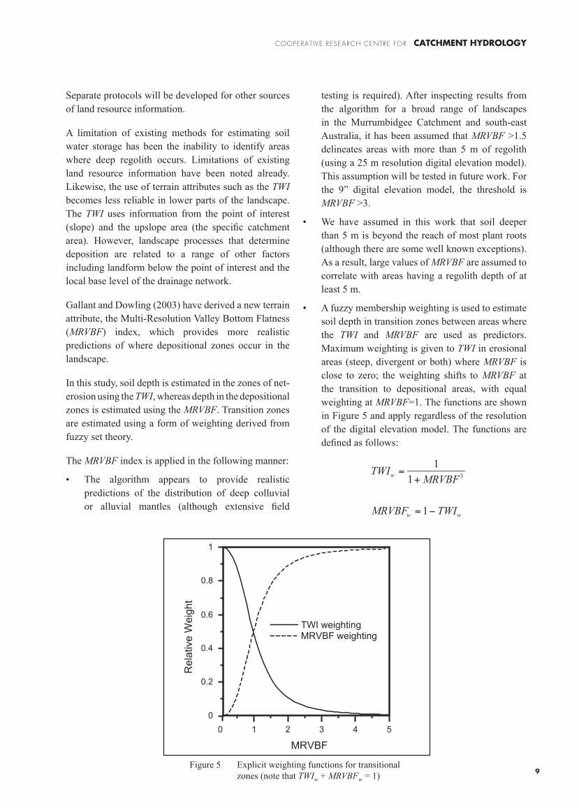
In this study, soil depth is estimated in the zones of net-erosion using the TWI, whereas depth in the depositional zones is estimated using the MRVBF. Transition zones are estimated using a form of weighting derived from fuzzy set theory.

The MRVBF index is applied in the following manner:

• The algorithm appears to provide realistic predictions of the distribution of deep colluvial or alluvial mantles (although extensive field

testing is required). After inspecting results from the algorithm for a broad range of landscapes in the Murrumbidgee Catchment and south-east Australia, it has been assumed that MRVBF >1.5 delineates areas with more than 5 m of regolith (using a 25 m resolution digital elevation model). This assumption will be tested in future work. For the 9” digital elevation model, the threshold is MRVBF >3.

• We have assumed in this work that soil deeper than 5 m is beyond the reach of most plant roots (although there are some well known exceptions). As a result, large values of MRVBF are assumed to correlate with areas having a regolith depth of at least 5 m.

• A fuzzy membership weighting is used to estimate soil depth in transition zones between areas where the TWI and MRVBF are used as predictors. Maximum weighting is given to TWI in erosional areas (steep, divergent or both) where MRVBF is close to zero; the weighting shifts to MRVBF at the transition to depositional areas, with equal weighting at MRVBF=1. The functions are shown in Figure 5 and apply regardless of the resolution of the digital elevation model. The functions are defined as follows:

��

��

�

� �

��

� �

��

�

�

Figure 5 Explicit weighting functions for transitional zones (note that TWIw + MRVBFw = 1)

� � � � � �

�

��

��

��

��

�

��

��

��


10

• For example, if the TWI has a weighting (TWIw) of 0.7, then the MRVBF by definition has a weighting (MRVBFw) of 0.3. If the predicted soil depth from the TWI function (TWIpred) at this point is 1.5 m, then the estimated depth is calculated as follows:

Depth = TWIw × TWIpred + MRVBFw × 5 = 0.7 × 1.5 m + 0.3 × 5 m = 2.5 m

2.2.2 A Horizon Thickness

Separate calculations for the available water store are normally required for the A and B horizons because the former normally store more water per unit depth than do B horizons. Deeper layers (e.g. buried soils, D horizons, C horizons and saprolite) also have contrasting storage capacities, but reliable data are rare. In this work, a simple two-layer soil profile has been assumed. Before this can be applied, a procedure is required for estimating A horizon thickness to complement the procedure for estimating total profile depth outlined above.

The Digital Atlas of Australian Soils and 1:100 000 soil-landscape maps provide estimates of the mean A horizon depth for each mapping unit. This cannot be readily adopted as a standard depth throughout the soil-mapping unit because shallow soils may be assigned a disproportionately thick A horizon (it may even exceed the estimated depth of the soil profile). An alternative strategy is to calculate the ratio of the A horizon depth to the median profile depth. However, this may return spurious results for deeper soils. Resolution of the problem requires some assumptions on geomorphic and pedogenic processes.

We have assumed that in landscapes where the rate of soil production limits sediment movement, soil profiles will thin towards crests. In a landscape where sediment transport capacity limits movement, soil profiles will not thin towards crests. These situations are illustrated in Figure 6.

We have made an initial assumption that supply-limited slopes dominate in landscapes with an annual rainfall <1000 mm in south-east Australia. This is a very

Figure 6 Patterns of soil depth on (a) slopes where sediment movement is limited by transport (typically areas with effective long-term groundcover, or high rates of soil production from weathering or aeolian deposition, or both) and (b) slopes where sediment movement is limited by supply (i.e. soil production is less than transport capacity)

��

��

��

��


11

tentative suggestion based on limited and qualitative observations in the Tumut region. We further assume that A horizon thickness varies with landscape position in erosional areas and that it has a more constant value in depositional areas. These assumptions will be tested in future studies.

The depth of A horizon has been estimated using the following procedure. The required input variables are the mean and shallowest depth of soil (d0 and d1 in Figure 4), and the mean A horizon depth (dµ) derived from the soil survey report. The procedure below assumes that soil thickness (di) has already been estimated for each grid cell (see results section):

• The A horizon thickness ratio (r) is calculated for each soil polygon where r = dµ / d1

• A horizon depth (dA) is calculated for all locations using:

dA = r di for r di < 2dµ

dA = 2di for r di ≥ 2dµ

If we had some assurance that dµ was an unbiased estimate of A horizon depth, then our procedure would introduce bias. However, very few land resource surveys use probabilistic sampling so the degree of bias is unknown in the first place. The approach is pragmatic but testing is required.

2.3 Water Retention

Estimates of water retention for the A and B horizons have been generated using two methods. Estimates for the Digital Atlas of Australian Soils have relied on McKenzie et al. (2000). These estimates are based on the pedotransfer functions of Williams et al. (1992) and relate to the dominant soil profile in each polygon. The available water capacity has been multiplied by the respective thickness of the A and B horizons and then summed. The B horizon thickness has been calculated as the total profile depth minus the A horizon thickness.

The water retention estimates derived from the 1:100 000 soil-landscape map of Chen and McKane (1996) use a more detailed analysis. Each soil-landscape polygon mapped by Chen and McKane (1996) usually has between one and four representative profiles defined with supporting measurements of water contents at –10 kPa and –1.5 MPa. The relative areas

of the representative profiles are also specified. The water retention measurements are usually available for at least two, and often three or four layers within the profile. Depth-weighted means have been calculated to produce an average value for the A and B horizons. Spatially-weighted means, using the areal percentage for each soil type, have then been calculated.

A correction has been made to the –10 kPa water contents in an attempt to offset the effect of measurement on sieved soil rather than an undisturbed core. It is assumed that the measured –10 kPa water content is actually representative of the –33 kPa value for undisturbed soil. The –10 kPa value for undisturbed soil is then estimated by linear interpolation (using log/log axes). This correction is based on observations by Loveday (1974) that –33 kPa water contents on sieved soil are often very close to the –10 kPa value for undisturbed cores. The correction results in a change of volumetric water content of only 1 or 2%. The results are presented in Table 1.


12

Tabl

e 1

D

ata

deri

ved

from

Che

n an

d M

cKan

e (1

996)

. The

wat

er r

eten

tion

estim

ates

are

bot

h de

pth-

wei

ghte

d an

d ar

ea-w

eigh

ted

aver

ages

. T

he s

calin

g pa

ram

eter

(X

i) is

an

area

-wei

ghte

d av

erag

e

��

��

��

� ��

� ��

��

��

��

��

��

� ��

��

��

��

��

��

��

��

��

��

��

��

��

��

��

��

��

��

��

��

��

��

��

��

��

��

��

��

��

��

��

��

��

��

��

��

��

��

��

��

��

��

��

��

��

��

��

��

��

��

��

��

��

��

��

��

��

��

��

��

��

��

��

��

��

��

��

��

��

��

��

��

��

��

��

��

��

��

��

��

��

��

��

��

��

��

��

��

��

��

��

��

��

��

��

��

��

��

��

��

��

��

��

��

��

��

��

��

��

��

��

��

��

��

��

��

��

��

��

��

��

��

��

��

��

��

��

��

��

��

��

��

��

��

��

��

��

��

��

��

��

��

��

��

��

��

��

��

��

��

��

��

��

��

��

��

��

��

��

��

��

��

��

��

��

��

��

��

��

��

��

��

��

��

��

��

��

��

��

��

��

��

��

��

��

��

��

��

��

��

��

��

��

��

��

��

��

��

��

��

��

��

��

��

��

��

��

��

��

��

��

��

��

��

��

��

��

��

��

��

��

��

��

��

��

��

��

��

��

��

��

��

��

��

��

��

��

��

��

��

��

��

��

��

��

��

��

��

��

��

��

��

��

��

��

��

��

��

��

��

��

��

��

��

��

��

��

��

��

��

��

��

��

��

��

��

��

��

��

��

��

��

��

��

��

��

��

��

��

��

��

��

��

��

��

��

��

��

��

��

��

��

��

��

��

��

��

��

��

��

��

��

��

��

��

��

��

��

��

��

��

��

��

��

��

��

��

��

��

��

��

��

��

��

��

��

��

��

��

��

��

��

��

��

��

��

��

��

��

��

��

��

��

��

��

��

��

��

��

��

��

��

��

��

��

��

��

��

��

��

��

��

��

��

��

��

��

��

��

��

��

��

��

��

��

��

��

��

��

��

��

��

��

��

��

��

��

��

��

��

��

��

��

��

��

��

��

��

��

��

��

��


13

3. Estimating Plant Available Water Capacity

The estimates of available water capacity (i.e. θ–10kpa — θ–1.5Mpa), whether measured directly or derived from pedotransfer functions, when summed over the depth of the profile are known to over-estimate the quantity of water actually extracted in field situations. The main problem is the diminishing ability of plants to extract water from deeper layers. This is due to both the physiology of the plant (e.g., annual crop versus deep-rooted woody perennial) and subsoil constraints to root growth. Published water extraction patterns across a range of soils and plant types (e.g., Williams 1983) suggest that a simple correction to the profile available water capacity can be made using a scaling factor that reflects root distribution.

3.1 Scaling Function to Reflect Root Density

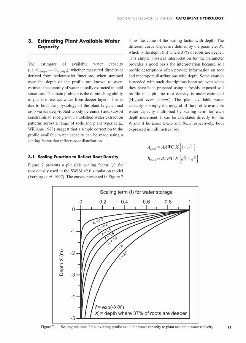
Figure 7 presents a plausible scaling factor ( f) for root density used in the SWIM v2.0 simulation model (Verburg et al. 1997). The curves presented in Figure 7

show the value of the scaling factor with depth. The different curve shapes are defined by the parameter Xi, which is the depth (m) where 37% of roots are deeper. This simple physical interpretation for the parameter provides a good basis for interpretation because soil profile descriptions often provide information on root and macropore distributions with depth. Some caution is needed with such descriptions because, even when they have been prepared using a freshly exposed soil profile in a pit, the root density is under-estimated (Hignett pers. comm.). The plant available water capacity is simply the integral of the profile available water capacity multiplied by scaling term for each depth increment. It can be calculated directly for the A and B horizons (ATotal and BTotal respectively, both expressed in millimetres) by:

Figure 7 Scaling relations for converting profile available water capacity to plant available water capacity

��

��

��

��

�

� ��

��

��

� ��

� ��

��

��

� ��

� ��

� ��

��

��

��

�

�

��

�

�

��

�

�

��

�

�

��

��

eeXBAWCB

eXAAWCA

ixid

ixAd

ixAd

iTotal

iTotal 1


14

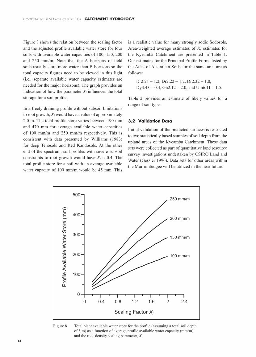
Figure 8 shows the relation between the scaling factor and the adjusted profile available water store for four soils with available water capacities of 100, 150, 200 and 250 mm/m. Note that the A horizons of field soils usually store more water than B horizons so the total capacity figures need to be viewed in this light (i.e., separate available water capacity estimates are needed for the major horizons). The graph provides an indication of how the parameter Xi influences the total storage for a soil profile.

In a freely draining profile without subsoil limitations to root growth, Xi would have a value of approximately 2.0 m. The total profile store varies between 190 mm and 470 mm for average available water capacities of 100 mm/m and 250 mm/m respectively. This is consistent with data presented by Williams (1983) for deep Tenosols and Red Kandosols. At the other end of the spectrum, soil profiles with severe subsoil constraints to root growth would have Xi ≈ 0.4. The total profile store for a soil with an average available water capacity of 100 mm/m would be 45 mm. This

is a realistic value for many strongly sodic Sodosols. Area-weighted average estimates of Xi estimates for the Kyeamba Catchment are presented in Table 1. Our estimates for the Principal Profile Forms listed by the Atlas of Australian Soils for the same area are as follows:

Dr2.21 = 1.2, Dr2.22 = 1.2, Dr2.32 = 1.0, Dy3.43 = 0.4, Gn2.12 = 2.0, and Um6.11 = 1.5.

Table 2 provides an estimate of likely values for a range of soil types.

3.2 Validation Data

Initial validation of the predicted surfaces is restricted to two statistically based samples of soil depth from the upland areas of the Kyeamba Catchment. These data sets were collected as part of quantitative land resource survey investigations undertaken by CSIRO Land and Water (Gessler 1996). Data sets for other areas within the Murrumbidgee will be utilized in the near future.

Figure 8 Total plant available water store for the profile (assuming a total soil depth of 5 m) as a function of average profile available water capacity (mm/m) and the root-density scaling parameter, Xi

� ��

�

��

��

��

��

��

��

��

��

��

��

��

��

��


15

Table 2 Suggested values of Xi for a select number of soil types (after Isbell 1996). Interpretations based largely on data provided by Williams (1983)

Soil type Xi Soil type XiStrongly Sodic Sodosols 0.4-0.7 Bleached Chromosols 1.4

Subnatric Grey and Yellow Sodosols 0.8 Grey VertosolsRed ChromosolsRed Kurosols

1.5

Subnatric Red Sodosols 1.0 Most DermosolsWell-structured Red Chromosols

1.6-1.8

Sodic Vertosols 0.8-1.3 Arenic Tenosols 1.9

Bleached Kurosols 1.3 Red Kandosols andRed Ferrosols

2.0


16


17

4. Results and Discussion

The estimated depth of soil is presented in Figures 9 and 10 for the Kyeamba Catchment. Figure 9 has been generated using the 9” DEM and the Digital Atlas of Australian Soils. Figure 10 has been generated using a fine resolution DEM (25 m grid cells) and 1:100 000 soil-landscape mapping (Chen and McKane 1996). The maximum depth has been arbitrarily set to 5 m.

Available water contents estimated using the 9” DEM and the Digital Atlas of Australian Soils are shown in Figure 11. Estimates using the 25 m resolution DEM and 1:100 000 soil-landscape maps are shown in Figure 12.

Figures 13 and 14 present predicted versus observed soil depths using the data of Gessler (1996). Predictions from the 9” DEM and the Digital Atlas of Australian Soils show little relationship with measured depths. This is primarily because the 9” digital elevation model cannot represent the fine-scale variation in topography responsible for the variations in soil depth as sampled by Gessler (1996). The relationships for the 25 m digital elevation model and the 1:100 000 soil-landscape map are generally quite good until depths of just over a metre when over-estimation appears to be a problem. However, it is difficult in this depth range to be sure whether bedrock has been reached or equipment refusal has occurred for other reasons. The drill rig used by Gessler relied on push-tubes and these can fail to reach bedrock because of coarse fragments or cemented layers. The large predicted depths mostly occur in the deeper soils – this is consistent with the

assumptions of the method and the suggestion that soil depth is under-estimated by conventional soil sampling methods. Conversely, the over-estimation may indicate that the weighting function is inappropriate.

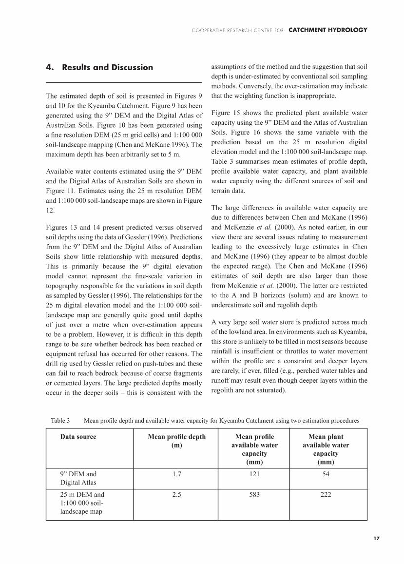
Figure 15 shows the predicted plant available water capacity using the 9” DEM and the Atlas of Australian Soils. Figure 16 shows the same variable with the prediction based on the 25 m resolution digital elevation model and the 1:100 000 soil-landscape map. Table 3 summarises mean estimates of profile depth, profile available water capacity, and plant available water capacity using the different sources of soil and terrain data.

The large differences in available water capacity are due to differences between Chen and McKane (1996) and McKenzie et al. (2000). As noted earlier, in our view there are several issues relating to measurement leading to the excessively large estimates in Chen and McKane (1996) (they appear to be almost double the expected range). The Chen and McKane (1996) estimates of soil depth are also larger than those from McKenzie et al. (2000). The latter are restricted to the A and B horizons (solum) and are known to underestimate soil and regolith depth.

A very large soil water store is predicted across much of the lowland area. In environments such as Kyeamba, this store is unlikely to be filled in most seasons because rainfall is insufficient or throttles to water movement within the profile are a constraint and deeper layers are rarely, if ever, filled (e.g., perched water tables and runoff may result even though deeper layers within the regolith are not saturated).

Table 3 Mean profile depth and available water capacity for Kyeamba Catchment using two estimation procedures

Data source Mean profile depth Mean profile Mean plant (m) available water available water capacity capacity (mm) (mm)

9” DEM and 1.7 121 54Digital Atlas

25 m DEM and 2.5 583 2221:100 000 soil-landscape map


18

Figure 13: Predicted and measured soil depths for the Griggward Study Area (Gessler 1996) using different terrain and soil map data sources (1:1 line shown).

Figure 14: Predicted and measured soil depths for the Ladysmith Study Area (Gessler 1996) using different terrain and soil map data sources (1:1 line shown).

Figure 9 Predicted soil depth using the 9" DEM and Atlas of Australian Soils for the Kyeamba Catchment


19

Figure 10 Predicted soil depth using the 25 m DEM and 1:100 000 soil landscape mapping for the Kyeamba Catchment


20

Figure 11 Predicted profile available water capacity using the 9″ DEM and Atlas of Australian Soils for the Kyeamba Catchment


21

Figure 12 Predicted profile available water capacity using the 25 m DEM and 1:100 000 soil landscape mapping for Kyeamba Catchment


22

� ��

�

�

�

�

�

�

� ��

� ��

�

��

��

��

��

��

��

��

��

��

��

�

�

�

�

�

�

�

��

��

��

��

��

��

�

��

��

��

��

��

��

��

��

�

�

�

�

�

�

�

�

�

� ��

��

��

��

��

��

��

��

�

� ��

�

�

�

�

�

�

� ��

� ��

�

��

��

��

��

��

��

��

��

��

��

�

�

�

�

�

�

�

��

��

��

��

��

��

�

��

��

��

��

��

��

��

��

�

�

�

�

�

�

�

�

�

� ��

��

��

��

��

��

��

��

�

Figure 13 Predicted and measured soil depths for the Griggward Study Area (Gessler 1996) using different terrain and soil map data sources (1:1 line shown)

Figure 14 Predicted and measured soil depths for the Ladysmith Study Area (Gessler 1996) using different terrain and soil map data sources (1:1 line shown)


23

Figure 15 Predicted plant available water capacity using the 9″ DEM and Atlas of Australian Soils for the Kyeamba Catchment


24

Figure 16 Predicted plant available water capacity using the 25 m DEM and 1:100 000 soil landscape mapping for Kyeamba Catchment


25

5. Directions

A scheme has been developed for providing more realistic estimates of water storage in soil than previously available from land resource survey data. The innovative method of terrain analysis appears to be robust and the procedure can be applied to large areas with relative ease. Most of the methodological uncertainties relate to the following:

• Data sets used to develop current pedotransfer functions (e.g. McKenzie et al. 2000) are derived from near surface measurements (i.e., A and B horizons). Very few data for other soil materials are available (e.g., C and D horizons, saprolite). A compilation of water retention measurements on these materials is required to develop better estimates of profile and plant available water capacity.

• Direct measurements of water storage in soil are available from several experimental sites in the Kyeamba Creek catchment (e.g. Book Book, Mona Vale, Ladysmith) and these will be used to test the methods proposed in this report.

• The validity of the arbitrary but explicit weighting functions for linking predictions of soil depth using the TWI and MRVBF index has to be examined for a range of landscapes.

• Minimal information is available on root distributions and soil-based limitations to root growth for perennials. This will be a major problem for modelling catchment responses to different systems of vegetation. The validity of the values used here for the scaling parameter (Xi) requires testing. Likewise a scheme for specifying Xi for annuals (e.g., crops, pastures and weeds) is needed. An interim would be to integrate profile available water capacity to 2 m rather than the 5 m used here for perennial vegetation.

• It would be valuable to compare the estimates of plant available water capacity with multi-temporal analyses of Landsat MSS data (e.g., using the Normalised Difference Vegetation Index) – the areas with large capacities should retain their greenness longer than surrounding lands.


26


27

6. References

Beckett PHT, Webster R (1971) Soil variability: a review. Soils and Fertilizers 34, 1-15.

Bouma J (1989) Using soil survey data for quantitative land evaluation. Advances in Soil Science 9, 177-213.

Chen XY, McKane DJ (1996) ‘Soil landscapes of the Wagga Wagga 1:100 000 sheet.’ Department of Land and Water Conservation, Sydney.

Gallant JC, Dowling TD (2003) A multi-resolution index of valley bottom flatness for mapping depositional areas. Water Resources Research (in press).

Gessler PE (1996) ‘Statistical soil-landscape modelling for environmental management.’ PhD Thesis, Australian National University.

Gessler PE, Moore ID, McKenzie NJ, Ryan PJ (1996) Soil-landscape modelling in southeastern Australia. In ‘GIS and environmental modeling: progress and research issues.’ (Eds. MF Goodchild, LT Steyaert, BO Parks, C Johnston, D Maidment, M Crane and S Glendinning) (GIS World Books: Fort Collins).

Heimsath, AM, Chappell J, Dietrich WE, Nishiizumi K, Finkel RC (2001) Late Quaternary erosion in southeastern Australia: a field example using cosmogenic nuclides Quaternary International 83-85, 169-185.

Hillel D (1998) ‘Environmental soil physics.’ (Academic Press: San Diego).

Isbell RF (1996) ‘The Australian soil classification.’ (CSIRO Publishing: Melbourne).

Jenkins BR (2000) ‘Soil landscapes of the Canberra 1:100 000 sheet.’ Department of Land and Water Conservation, Sydney.

McKenzie NJ, Jacquier DW, Ashton LJ, Cresswell HP (2000) ‘Estimation of soil properties using the Atlas of Australian Soils.’ CSIRO Land & Water Technical Report 11/00, Canberra.

McKenzie NJ, Cresswell HP (2002) Estimating soil physical properties using more readily available data. In ‘Soil physical measurement and interpretation for land evaluation.’ (Eds NJ McKenzie, KJ Coughlan, HP Cresswell) Australian Soil and Land Survey Handbook Series No. 5 (CSIRO Publishing: Melbourne).

McKenzie NJ, Hook J (1992) Interpretations of the Atlas of Australian Soils. Consulting Report to the Environmental Resources Information Network (ERIN). CSIRO Division of Soils Technical Report 94/1992.

McKenzie NJ, Ryan, PJ (1999). Spatial prediction of soil properties using environmental correlation. Geoderma 89, 67-94.

NLWRA (2001) ‘Australian agriculture assessment 2001.’ National Land and Water Resources Audit, Canberra.

Northcote KH (1979) ‘A factual key for the recognition of Australian soils.’ 4th Edn. (Rellim Tech. Publ: Glenside, S.A.).

Northcote KH with Beckmann GG, Bettenay E, Churchward HM, Van Dijk DC, Dimmock GM, Hubble GD, Isbell RF, McArthur WM, Murtha GG, Nicolls KD, Paton TR, Thompson CH, Webb AA, Wright MJ (1960-1968) ‘Atlas of Australian Soils, Sheets 1 to 10. With explanatory data (CSIRO Aust. and Melbourne University Press: Melbourne).

Pillans B (1999) Soil development at a snail’s pace: evidence from a 6 Ma soil chronosequence on basalt in north Queensland, Australia. Geoderma 80, 117-128.

Walker PH, Butler BE (1983) Fluvial processes. In ‘Soils: an Australian viewpoint.’ (CSIRO: Melbourne/ Academic Press: London).

Wilding LP, Drees LR (1983) Spatial variability and pedology. In ‘Pedogenesis and Soil Taxonomy. I Concepts and interactions.’ (Eds LP Wilding, NE Smeck and GF Hall) Developments in Soil Science 11A (Elsevier: Amsterdam).

Williams J, Ross PJ, Bristow KL (1992) Prediction of the Campbell water retention function from texture, structure and organic matter. In ‘Indirect methods for estimating the hydraulic properties of unsaturated soils.’ (Eds. MTh van Genuchten, FJ Leij and LJ Lund) (University of California: Riverside).

The Cooperative Research Centre for Catchment Hydrology is a cooperative venture formed under the Commonwealth CRCProgram between:

•Brisbane City Council

•Bureau of Meteorology

•CSIRO Land and Water

•Department of Infrastructure, Planning and NaturalResources, NSW

•Department of Sustainability and Environment, Vic

•Goulburn-Murray Water

•Griffith University

CENTRE OFFICE

Department of Civil Engineering Building 60 Monash University VIC 3800 AustraliaTelephone +61 3 9905 2704 Facsimile +61 3 9905 5033 Email [email protected] www.catchment.crc.org.au

•Melbourne Water

•Monash University

•Murray-Darling Basin Commission

•Natural Resources and Mines, Qld

•Southern Rural Water

•The University of Melbourne

•Wimmera Mallee Water

C O O P E R A T I V E R E S E A R C H C E N T R E F O R C A T C H M E N T H Y D R O L O G Y

Associate:

• Water Corporation of Western Australia

Established and supportedunder the Australian

Government’s CooperativeResearch Centre Program

estimating water storage capacities in soil at catchment scales

Documents