estimating tropical cyclone intensity in the south china

atmosphere

Article

Estimating Tropical Cyclone Intensity in the SouthChina Sea Using the XGBoost Model and FengYunSatellite Images

Qingwen Jin 1,2, Xiangtao Fan 1,3, Jian Liu 1,3,*, Zhuxin Xue 4 and Hongdeng Jian 1

1 Key Laboratory of Digital Earth Science, Aerospace Information Research Institute, Chinese Academy ofSciences, Beijing 100094, China; [email protected] (Q.J.); [email protected] (X.F.); [email protected] (H.J.)

2 University of Chinese Academy of Sciences, Beijing 100049, China3 Hainan Key Laboratory of Earth Observation, Sanya 572029, China4 Beijing Jinghang Computation and Communication Research Institute, Beijing 100074, China;

[email protected]* Correspondence: [email protected]

Received: 20 March 2020; Accepted: 20 April 2020; Published: 22 April 2020��

Abstract: Conventional numerical methods have made significant advances in forecasting tropicalcyclone (TC) tracks, using remote sensing data with high spatial and temporal resolutions. However,over the past two decades, no significant improvements have been made with regard to the accuracyof TC intensity prediction, which remains challenging, as the internal convection and formationmechanisms of such storms are not fully understood. This study investigated the relationship betweenremote sensing data and TC intensity to improve the accuracy of TC intensity prediction. An intensityforecast model for the South China Sea was built using the eXtreme Gradient Boosting (XGBoost)model and FengYun-2 (FY-2) satellite data, environmental data, and best track datasets from 2006 to2017. First, correlation analysis algorithms were used to extract the TC regions in which the satellitedata were best correlated, with TC intensity at lead times of 6, 12, 18, and 24 h. Then, satellite, besttrack, and environmental data were used as source data to develop three different XGBoost modelsfor predicting TC intensity: model A1 (climatology and persistence predictors + environmentalpredictors), model A2 (A1 + satellite-based predictors extracted as mean values), and model A3(A1 + satellite-based predictors extracted by our method). Finally, we analyzed the impact of the FY-2satellite data on the accuracy of TC intensity prediction using the forecast skill parameter. The resultsrevealed that the equivalent blackbody temperature (TBB) of the FY-2 data has a strong correlationwith TC intensity at 6, 12, 18, and 24 h lead times. The mean absolute error (MAE) of model A3 wasreduced by 0.47%, 1.79%, 1.91%, and 5.04% in 6, 12, 18, and 24 h forecasts, respectively, relative tothose of model A2, respectively, and by 2.73%, 7.58%, 7.64%, and 5.04% in 6, 12, 18, and 24 h forecasts,respectively, relative to those of model A1. Furthermore, the accuracy of TC intensity prediction isimproved by FY-2 satellite images, and our extraction method was found to significantly improveupon the traditional extraction method.

Keywords: satellite data; South China Sea; tropical cyclone intensity; XGBoost

1. Introduction

Over the past 20 years, the use of numerical weather prediction models has improved theforecast accuracy of tropical cyclone (TC) track by about 50% for lead times of 24–72 h [1]. One ofthe main reasons for this improved accuracy is the use of high resolution remote sensing data.Satellite data are very important in the accurate tracking of fast-moving TCs, because they containeffective observational information for optimizing the initial numerical prediction field. Furthermore,

Atmosphere 2020, 11, 423; doi:10.3390/atmos11040423 www.mdpi.com/journal/atmosphere

http://www.mdpi.com/journal/atmosphere

http://www.mdpi.com

https://orcid.org/0000-0002-7441-659X

http://www.mdpi.com/2073-4433/11/4/423?type=check_update&version=1

http://dx.doi.org/10.3390/atmos11040423

http://www.mdpi.com/journal/atmosphere

Atmosphere 2020, 11, 423 2 of 22

high-spatiotemporal-resolution satellite measurements can provide observational data for areas lackingground observational data [2]. For example, cloud data from satellite images have been employed toimprove the accuracy of numerical prediction [3], and wind information contained in satellite datahas been employed to improve TC forecast accuracy [4]. Despite the advancements in the use ofnumerical models, the past two decades have seen little improvement in the accuracy of TC intensityprediction for lead times of 24–72 h [5], and although meaningful improvements have been seen in TCintensity forecasting, such forecasting remains challenging, as the internal convection and formationmechanisms of such storms are not fully understood [6].

In addition to conventional numerical methods, the statistical-dynamical approach has been usedas an operational guide for TC intensity prediction. The “statistical hurricane prediction scheme”(SHIPS) has used this approach successfully in the North Atlantic and East Pacific to predict TCintensity [7]. The first version of the “statistical typhoon intensity forecasting scheme” (STIPS) wasdeveloped by Knaff et al. [8] in 2002, to predict TC intensity based on the SHIPS. In 2003, the STIPSwas improved and applied in operational settings. Following this, Gao and Chiu [9] attempted topredict TC intensity using an artificial neural network-based method; they proved that the accuracy ofa scheme using neural network models was superior to that of one using multiple linear regressionmodels, leading to the recent adoption of this method to predict TC intensity. In another study, inwhich the intensity of TCs was forecast using a radial-basis function network (RBFN), multilayerperceptron (MLP) model, and statistical multiple linear and ordinary linear regression [10], the MLPmodel was found to have the lowest forecasting error. Chandra and Dayal [11], predicted cyclonewind intensity in the South Pacific region using Elman recurrent neural networks, and Chaudhuri etal. [12] found a double hidden layer neural network to be more accurate than a single-layer networkfor forecasting typhoon intensity. Thus, as described above, most researchers use a non-linear modelto predict TC intensity.

Given the advancements in satellite data, some researchers investigated the use of satellite data inTC intensity forecasting [13]. TC intensity in the North Indian Ocean was predicted by incorporatingaverage values from satellite data into a set of predictors, and it was found that the addition of satellitedata improved the prediction model [11]. Gao et al. predicted TC intensity using a decision tree andsatellite data; they showed that employing the ocean coupling potential intensity index with satellitedata reduced the accuracy of the TC intensity prediction [13]. The satellite predictors were extractedas area-averaged data, extracting detailed information using the mean results in the details beinghidden or diluted. The satellite data are particularly rich around the center of the TC, and this data candescribe the convective characteristics affecting TC intensity [14]. Wang [15] suggested that convectionnear the TC center is a key feature of overall convection in tropical cyclogenesis and that the spatialpattern of the convection intensity might also be important. Given such findings, a new extractionmethod that can comprehensively glean TC intensity information from remote sensing data couldimprove TC intensity prediction [16].

In recent years, some scholars have shown that the decision tree method can improve theaccuracy of the TC intensity prediction. TC intensity in the western North Pacific was predictedusing the decision tree method [17]. The theory and application of the decision tree method havedeveloped significantly since Chen’s proposal of the eXtreme Gradient Boosting (XGBoost) model [18];this model has been applied in several studies, on topics including image classification [19], speechrecognition [20], and biomedical studies [21]. The XGBoost model has also proved to be useful inpredicting TC intensity [22]. TC intensity is affected by several factors that are often ambiguous anduncertain. In this study, we used the XGBoost model to predict TC intensity, because its algorithmcan handle many dimensions and be used to conduct multi-factor predictions. Factor mining hasproved to be useful in forecasting model constructions [23,24]. The XGBoost model can also be usedin conjunction with factor mining, which has proved to be useful in forecasting model construction.Furthermore, another advantage of the XGBoost model is its very low computational cost for userswith a basic knowledge of TCs.

Atmosphere 2020, 11, 423 3 of 22

Therefore, we focused on using satellite predictors extracted via a new method, to establish amachine learning model for predicting TC intensity. This study aimed to establish an XGBoost-basedframework to predict TC intensity in the South China Sea, using data from the China MeteorologicalAdministration–Shanghai Typhoon Institute (CMA-STI) [25], meteorological variables from theEuropean Centre for Medium-Range Weather Forecasts (ECMWF) [26], and satellite data fromthe National Satellite Meteorological Center FengYun Satellite Data Center, covering the period of2006–2017. The differences between the predicted and observed data were used to analyze the dynamicsof TC intensity development. The primary objectives of this study were: (1) to establish a South ChinaSea TC intensity prediction model based on the XGBoost framework and satellite-based potentialpredictors; (2) to analyze the influence of the FengYun-2 (FY-2) remote sensor data on TC intensityforecast results, and (3) to analyze the influence of the satellite data extraction method used on TCintensity forecast results.

2. Materials and Methods

We considered three types of potential predictors—satellite, best track, and environmentaldata—to establish a South China Sea TC intensity model, based on the framework shown in Figure 1.We prepared all the data and the theoretical basis for our models as described in Sections 2.1 and 2.2.The formulation of the TC intensity prediction model is presented in Section 2.3.

Atmosphere 2020, 10, x FOR PEER REVIEW 3 of 22

Administration–Shanghai Typhoon Institute (CMA-STI) [25], meteorological variables from the European Centre for Medium-Range Weather Forecasts (ECMWF) [26], and satellite data from the National Satellite Meteorological Center FengYun Satellite Data Center, covering the period of 2006–2017. The differences between the predicted and observed data were used to analyze the dynamics of TC intensity development. The primary objectives of this study were: (1) to establish a South China Sea TC intensity prediction model based on the XGBoost framework and satellite-based potential predictors; (2) to analyze the influence of the FengYun-2 (FY-2) remote sensor data on TC intensity forecast results, and (3) to analyze the influence of the satellite data extraction method used on TC intensity forecast results.

2. Materials and Methods

We considered three types of potential predictors—satellite, best track, and environmental data—to establish a South China Sea TC intensity model, based on the framework shown in Figure 1. We prepared all the data and the theoretical basis for our models as described in Section 2.1 and Section 2.2. The formulation of the TC intensity prediction model is presented in Section 2.3.

Figure 1. Flowchart of proposed TC intensity prediction model.

2.1. Data

The South China Sea was chosen as the study area for three reasons. Firstly, TCs in the South China Sea include those generated locally and those that travel into the South China Sea from the western North Pacific Ocean [27]. Secondly, the accuracy of South China Sea TC track predictions in 2018 was significantly higher than that in 2017, but the accuracy of TC intensity predictions did not significantly improve in this time period [28]. Finally, several TCs with concentrated landing times have affected coastal areas of the South China Sea, and such storms may induce serious secondary disasters [29].

The datasets used in this study, including their spatial and temporal resolutions and temporal coverage, are described in Table 1. Owing to the limitations of satellite data transmission time, the data used in this study relating to TCs and their surrounding environments in the South China Sea were limited to the period of 2006–2017. To ensure a well-constructed model, the ratio of training samples to experimental samples was approximately 7:3. TC data from 2006 to 2012 were selected for use as training samples and data from 2013 to 2017 were selected as the experimental samples. All TCs considered had been generated in or had entered the study area (105° E to 120° E, 10° N to 25° N) and had a minimum lifetime of 48 hours. The number of samples selected for each lead time is listed in Table 2.

Table 1. Dataset characteristics.

Dataset Spatial Resolution Temporal Resolution Spatial Coverage Temporal Coverage CMA-STI 0.1° 6 h Northwest Pacific 1949–2017

ERA Interim 1° × 1° 6 h Global 1979–2017

TBB FY-2C 0.05° × 0.05° 1 h Global 2006–2009 FY-2E 0.05° × 0.05° 1 h Global 2010–2017 FY-2G 0.05° × 0.05° 1 h Global 2015–2017

Note: TBB = blackbody temperature.

Figure 1. Flowchart of proposed TC intensity prediction model.

2.1. Data

The South China Sea was chosen as the study area for three reasons. Firstly, TCs in the SouthChina Sea include those generated locally and those that travel into the South China Sea from thewestern North Pacific Ocean [27]. Secondly, the accuracy of South China Sea TC track predictions in2018 was significantly higher than that in 2017, but the accuracy of TC intensity predictions did notsignificantly improve in this time period [28]. Finally, several TCs with concentrated landing timeshave affected coastal areas of the South China Sea, and such storms may induce serious secondarydisasters [29].

The datasets used in this study, including their spatial and temporal resolutions and temporalcoverage, are described in Table 1. Owing to the limitations of satellite data transmission time, the dataused in this study relating to TCs and their surrounding environments in the South China Sea werelimited to the period of 2006–2017. To ensure a well-constructed model, the ratio of training samplesto experimental samples was approximately 7:3. TC data from 2006 to 2012 were selected for useas training samples and data from 2013 to 2017 were selected as the experimental samples. All TCsconsidered had been generated in or had entered the study area (105◦ E to 120◦ E, 10◦ N to 25◦ N) andhad a minimum lifetime of 48 hours. The number of samples selected for each lead time is listed inTable 2.

Atmosphere 2020, 11, 423 4 of 22

Table 1. Dataset characteristics.

Dataset SpatialResolution

TemporalResolution Spatial Coverage Temporal

Coverage

CMA-STI 0.1◦ 6 h Northwest Pacific 1949–2017ERA Interim 1◦ × 1◦ 6 h Global 1979–2017

TBBFY-2C 0.05◦ × 0.05◦ 1 h Global 2006–2009FY-2E 0.05◦ × 0.05◦ 1 h Global 2010–2017FY-2G 0.05◦ × 0.05◦ 1 h Global 2015–2017

Note: TBB = blackbody temperature.

Table 2. Number of TC training and test samples used for 6, 12, 18, and 24 h lead-time assessments.

Lead Time (h) All Samples (2006–2017) Training Samples(2006–2012)

Test Samples(2013–2017)

6 1164 770 39412 1041 697 34418 922 625 29724 808 557 251

The CMA-STI best track dataset includes the TC position (latitude and longitude), TC intensitycategory, minimum pressure near the TC center, and 2 min mean maximum sustained wind near theTC center. The 2006–2017 South China Sea TC datasets were downloaded from the CMA-STI best trackdataset covering the western North Pacific (http://www.typhoon.gov.cn/) [25].

The environmental datasets were drawn from the ECMWF Re-Analysis (ERA-Interim) dataset [30].This dataset provides assimilation analysis data four times daily at 00:00, 06:00, 12:00, and 18:00.Its spatial resolution is 1◦ × 1◦. We selected environmental variables including relative humidity,temperature, divergence, and u- and v-wind at 200, 250, 300, 350, 400, 450, 500, 700, 750, 775, 800, 825,and 850 hPa. The maximum potential intensity (MPI) was estimated using sea surface temperaturefrom the ERA-Interim dataset and CMA-STI best track dataset.

Remote sensing satellite data can provide high-precision meteorological information for TCintensity prediction [2]. In this study, satellite datasets were used to identify a convective intensityfeature. The visible and infrared spin scan-radiometer sensor used on the CMA’s FY satellites is ascanning instrument that provides measurements of oceanic and atmospheric parameters relevant toregional water and energy cycles [31–33]. As different FY-series satellites operated during 2006–2017,data from the FY-2C, FY-2E, and FY-2G sensors were selected to cover the entire study period.The FY-2C satellite instrument was launched on October 19, 2004 and ceased operations on December28, 2009, and the temporal coverage of the available data extended from May 2005 to January2010. The FY-2E satellite instrument was launched on June 15, 2008 and ceased operations onJune 2, 2015; the temporal coverage of the available data was from December 2009 to January2019. The FY-2G satellite instrument was launched on June 3, 2015, and the temporal coverageof its available data extends from June 2015 to present. The FY-2 data obtained for this studywere downloaded from the National Satellite Meteorological Center FengYun Satellite Data Center(http://satellite.nsmc.org.cn/PortalSite/Data/Satellite.aspx) [34]. The selected satellite product wasthe blackbody temperature (TBB), which represents the most primitive observational data for cloudformation and display enhancement.

2.2. Methods

2.2.1. XGBoost Theoretical Framework

The XGBoost model is a heavy end-to-end promoting tree system, that is improved based on agradient-boosting decision tree algorithm [18]. XGBoost is an ensemble method that can integrate

http://www.typhoon.gov.cn/

http://satellite.nsmc.org.cn/PortalSite/Data/Satellite.aspx

Atmosphere 2020, 11, 423 5 of 22

several weak learners into a powerful learner for prediction. XGBoost aims to prevent overfittingand decrease the cost of computing resources, by reducing the objective function using regularizationterms. The prediction process using the XGBoost model is presented in Figure 2.Atmosphere 2020, 10, x FOR PEER REVIEW 5 of 22

Figure 2. Principles of the XGBoost algorithm used as a predictive model.

The XGBoost model generates a strong ensemble regression tree, through the combination of several weak regression trees. Firstly, according to the principles and requirements of the XGBoost model, we organized the training sample set, defined the objective function ( ), and selected a number of iterations (n) for model training. Secondly, the first derivative = , and second derivative ℎ =, (calculated before the training) were summed, generating ( and ). Thirdly, to prevent overfitting, we employed regularization and obtained a new objective function ∗ =− ∑ + . Fourth, we added a new tree to the original tree = ∑ ( ) = + ( ). After many iterations, the model’s ensemble regression trees were formed.

2.2.2. Embedded Selection Algorithm

Among the many predictors, predictor information is sometimes duplicated, and some predictors were not related to TC intensity. As inputting irrelevant predictors or predictors with repetitive information into the model reduces the model’s generalization ability, the embedded selection algorithm was used to select satellite predictors and remove irrelevant and duplicate predictors. Feature selection is automatically performed during the learning process of the algorithm, which can compensate for the shortcomings of the encapsulated and filtered feature selection algorithms. We used the learning model (XGBoost) to select the most valuable predictors for subsequent model design.

2.3. Formulation of the TC Intensity Prediction Model

A model for predicting the TC intensity in the South China Sea was established by applying XGBoost to FengYun satellite images. The predictor extraction and parameter adjustment methods employed in the TC intensity prediction model are discussed in Sections 2.3.1 and 2.3.2, respectively, and our experimental design is presented in Section 2.3.3.

2.3.1. Predictor Extraction Method

This study aimed to develop a machine learning model for predicting TC intensity in the South China Sea, at lead times of 6, 12, 18, and 24 h. Climatology and persistence (CLIPER), environmental,

Figure 2. Principles of the XGBoost algorithm used as a predictive model.

The XGBoost model generates a strong ensemble regression tree, through the combination ofseveral weak regression trees. Firstly, according to the principles and requirements of the XGBoostmodel, we organized the training sample set, defined the objective function (Obj), and selected anumber of iterations (n) for model training. Secondly, the first derivative gi = ∂y̌i

m−1 l(yi, y̌i

m−1)

and

second derivative hi = ∂2y̌i

m−1 l(yi, y̌i

m−1)

(calculated before the training) were summed, generating

(G j and H j). Thirdly, to prevent overfitting, we employed regularization and obtained a new

objective function obj∗ = − 12

N∑j=1

G jH j+θ

+ ϕN. Fourth, we added a new tree to the original tree

y̌im =

T∑t=1

ft(xi) = y̌im−1 + ft(xi). After many iterations, the model’s ensemble regression trees

were formed.

2.2.2. Embedded Selection Algorithm

Among the many predictors, predictor information is sometimes duplicated, and some predictorswere not related to TC intensity. As inputting irrelevant predictors or predictors with repetitiveinformation into the model reduces the model’s generalization ability, the embedded selectionalgorithm was used to select satellite predictors and remove irrelevant and duplicate predictors.Feature selection is automatically performed during the learning process of the algorithm, which cancompensate for the shortcomings of the encapsulated and filtered feature selection algorithms. We usedthe learning model (XGBoost) to select the most valuable predictors for subsequent model design.

Atmosphere 2020, 11, 423 6 of 22

2.3. Formulation of the TC Intensity Prediction Model

A model for predicting the TC intensity in the South China Sea was established by applyingXGBoost to FengYun satellite images. The predictor extraction and parameter adjustment methodsemployed in the TC intensity prediction model are discussed in Sections 2.3.1 and 2.3.2, respectively,and our experimental design is presented in Section 2.3.3.

2.3.1. Predictor Extraction Method

This study aimed to develop a machine learning model for predicting TC intensity in the SouthChina Sea, at lead times of 6, 12, 18, and 24 h. Climatology and persistence (CLIPER), environmental,and satellite-based predictors were used as input variables for the XGBoost model, and the outputvariable was TC intensity change.

Climatology and Persistence (CLIPER) Factors

Both linear and non-linear models have been built using CLIPER predictors to simulate TCintensity changes [35,36]. The CLIPER parameters values are computed in terms of TC location,pressure, and time of the year. To select relevant climatology and persistence factors, motion featuresand climatology and persistence factors at the initial time and during the previous period are described.The climatology and persistence variables used in this study were the same as those used by Baik [36]and Zhu [37], and because the month of occurrence of the TC and the intensity category of the TCaffect the TC intensity, we added month and intensity categories based on the predictors proposed byZhu [37]. The CLIPER predictors used in this study are given in Table 3. Following this preliminaryselection, a set of potential CLIPER predictors for TC intensity at each lead time (6, 12, 18, and 24 h)was chosen. To fully show the effects of the CLIPER predictors, we established square terms basedon the existing CLIPER factors. In addition to the predictors in Table 3, other potential predictors aredescribed in Jin [22].

Table 3. Climatology and persistence, environmental, and satellite-based predictors used in this study.

Predictors Description

Climatology and PersistenceLatitude Latitude 0, 6, 12, 18, and 24 h ahead

Longitude Longitude 0, 6, 12, 18, and 24 h aheadMinimum pressure near the tropical cyclone (TC)

centerMinimum pressure near the TC center 0, 6, 12, 18, and 24 h

ahead2 min mean maximum sustained wind near the TC

center2 min mean maximum sustained wind near the TC center 0, 6,

12, 18, and 24 h aheadMonth Month of TC 0, 6, 12, 18, and 24 h ahead

Intensity category TC intensity category 0, 6, 12, 18, and 24 h ahead

Environmental Factors

MPI Maximum potential intensity based on equation (1) belowRHLO Area-averaged (200–800 km) relative humidity at 700–850 hPaRHHI Area-averaged (200–800 km) relative humidity at 300–500 hPaU200 Area-averaged (200–800 km) zonal wind at 200 hPaT200 Area-averaged (0–1000 km) temperature at 200 hPaD200 Area-averaged (200–800 km) divergence at 200 hPaSHRS Area-averaged (200–800 km) 500–850 hPa wind shearSHRD Area-averaged (200–800 km) 200–850 hPa wind shear

USHRS Area-averaged (200–800 km) 500–850 hPa zonal wind shearUSHRD Area-averaged (200–800 km) 200–850 hPa zonal wind shear

Vr850 Area-averaged (0–1000 km) 850 hPa relative vorticity

Satellite-based Factors

TBB Equivalent blackbody temperature

Atmosphere 2020, 11, 423 7 of 22

Environmental Factors

Table 3 also presents the environmental variables used in the study. Environmental factors wereobtained according to the “perfect prog” theory [8,38]. Perfect prog is an ideal application environment,which generally uses a multiple linear regression model to process the output of a numerical model,which in this case is the predictors. In the experimental stage, we use reanalysis data to replace theoutput of the numerical model. The environmental factors selected in this study were divided intothree categories, including factors related to sea surface temperature, moisture fields, and wind fields.The values for the first category were drawn from the ERA-Interim dataset and were interpolated intothe TC center, and those for the latter two categories were averaged around the center.

Sea surface temperature (SST) primarily serves to estimate the upper bound of TC intensity.The best indicator to describe the upper bound of TC intensity is MPI. MPI values can be calculatedtheoretically [39–41] or empirically [8,39,42]. The empirical method was selected based on the approachof DeMaria and Kaplan [39]. The SST selected from the ERA-Interim dataset was interpolated to theTC center according to the best track data from 2006–2017, to determine the relationship between SSTand TC intensity [9], as follows:

MPI = A + BeC(T−T0) (1)

The values were set as follows: A = 17.76 m/s, B = 49.69 m/s, C = 0.1218 ◦C−1, and T0 = 30.0 ◦C.The maximum value of MPI was 75 m/s. The CMA-STI best track dataset and 2 min sustained maximumwind speed were used to compute the correlation coefficient in our study, whereas Knaff used theJTWC best track dataset and 1 min sustained maximum wind speed to estimate the coefficient.

Because convection is the direct power source for a TC, variations in relative humidity can affectthe TC intensity [9]. The average relative humidity at 700, 750, 800, and 850 hPa (RHLO); averagerelative humidity at 300, 400, 450, and 500 hPa (RHHI); zonal wind at 200 hPa (U200); temperature at200 hPa (T200); divergence at 200 hPa (D200); relative vorticity at 850 hPa (Vr850); average zonal windshear at 500, 700, 750, 800, and 850 hPa (USHRS); and average wind shear at 200, 250, 300, 400, 450, 500,700, 750, 800, and 850 hPa (USHRD) were chosen as the environmental predictors to assess the potentialimpact of moisture and wind fields on TC intensity. As vertical wind shear has also been found tobe crucial in predicting TC intensity [9,36,43], we considered two additional factors, defined as thedifference between the 850 and 200 hPa horizontal wind vectors (SHRS) and the difference betweenthe 850 and 500 hPa horizontal wind vectors (SHRD). We applied an environmental factor extractionmethod, based on the approach of Gao and Knaff [8,9,44]. To fully show the effects of environmentalfactors, we established some square and cubic terms based on the existing factors [8,9]. In addition tothe predictors in Table 3, other potential predictors are described in Jin [22].

Satellite-Based Factors

The relationship between TBB and TC intensity has previously been quantified [45–47].Weatherford and Gray [48] showed that TCs have fast outer-core winds that restrict inflow to theeye-wall; based on their results, Mundell [49] noted that a high ratio of inner-to outer-core convectionindicates future intensification, as this suggest that the inner-core processes dominate over outer-coreprocesses. Based on these findings, Fitzpatrick [47] showed in a study of TBB ranges from 0–6◦ inintervals of 1◦ that TBB data contain additional important convection information. Chen [45] appliedpredictors, including max, min, and mean TBB, within spatial regions to predict TC intensity. Chen’sfindings regarding TBB, however, applied characteristics identified in earlier literature and producedno uniform law. To extract TBB features more precisely and accurately, we designated a spatial regionbased on a correlation coefficient. The 0.05◦ × 0.05◦ resolution of the FengYun satellite data used in thisstudy is quite different from those used in previous studies and offers more detailed TBB information.

We analyzed the correlation between the satellite data and TC intensity. In Figure 3a, which showsthe correlation coefficients (CCs) between TC intensity and TBB, there is a negative correlation in mostareas; in other words, a lower TBB indicates stronger convection. Figure 3b–e show the maximum CCs

Atmosphere 2020, 11, 423 8 of 22

between contemporary TBB data in the region and TC intensities at 6, 12, 18, and 24 h lead times, whichwere −0.56, −0.52, −0.47, and −0.41, respectively. The CCs between the TBB of the TC center and the TCintensity became smaller with longer lead times. Figure 3b–e show significantly negative correlationsin areas spreading to the west as the lead time extended. The most important part of each figure is itscenter, corresponding to the clearly visible eye of the TC, at which the absolute value of the CC was lessthan the absolute value of the CC in the surrounding areas. This phenomenon suggests that the CCin the eye decreases with longer lead times. TBB data obtained from IR (infrared radiation) imagerycontain important information regarding TC intensity. The figures show that negative correlationsoccurred at approximately 4◦ around each TC center, which was used to determine the TBB selectionarea radius of 4◦ in the next step.


figures show that negative correlations occurred at approximately 4° around each TC center, which was used to determine the TBB selection area radius of 4° in the next step.

Figure 3. Correlations between South China Sea tropical cyclone (TC) intensity at various forecast lengths and the surrounding equivalent blackbody temperature (TBB). The center of each figure corresponds to the center of the TC. Forecast lengths depicted are (a) 0, (b) 6, (c) 12, (d) 18, (e) and 24 h.

We then extracted satellite-based predictors from the TBB images in Figure 4. Fitzpatrick [47] established radial areas of 0–1°, 0–2°, 0–4°, 0–6°, 1–2°, 2–4°, and 2–6°, with TBBs ranging from 193–218 K in 5 K increments. An examination of Figure 3 reveals that negative correlations were primarily distributed at 4° around the TC center. In our adaptation of Fitzpatrick’s methods, we processed radial annuli over 0–4°from the TC center in 0.1° increments. The corresponding TBB measurements were extracted from each of the 40 annuli. This approach allowed us to extract information regarding the TC in greater detail and to address the phenomenon of TC convection. Table 4 presents descriptions of the TBB-extracted factors. GAPRxTb_N represents the number of pixels in each radial area colder than a specified TBB, where Rx indicates the radial increment, Tb indicates the TBB value (193 K, 198 K, 203 K, 208 K, 213 K, and 218 K), and N indicates the location of rings. For example, the number of pixels in a 0–0.1° radial area that were colder than 193 K are denoted as GAP0206_1, and the number of pixels in a 2–2.1° radial area that were colder than 208 K are denoted GAP0206_21. GAP02max_N indicates the maximum TBB in each spatial area; for example, the maximum TBB in a 0–0.1° radial area is designated GAP02max_1. GAP02min_N indicates the minimum TBB in each radial area; for example, the minimum TBB in a 0–0.1° radial area is termed GAP02min_1. Similarly, GAP02mean_N indicates the mean TBB in each radial area; for example, the mean TBB in a 0–0.1° radial area is designated as GAP02mean_1. Finally, the differences between the TBB value of the center and the maximum and minimum values are designated as GAP02maxc_N and GAP02minc_N, respectively.

Figure 3. Correlations between South China Sea tropical cyclone (TC) intensity at various forecastlengths and the surrounding equivalent blackbody temperature (TBB). The center of each figurecorresponds to the center of the TC. Forecast lengths depicted are (a) 0, (b) 6, (c) 12, (d) 18, (e) and 24 h.

We then extracted satellite-based predictors from the TBB images in Figure 4. Fitzpatrick [47]established radial areas of 0–1◦, 0–2◦, 0–4◦, 0–6◦, 1–2◦, 2–4◦, and 2–6◦, with TBBs ranging from 193–218 Kin 5 K increments. An examination of Figure 3 reveals that negative correlations were primarilydistributed at 4◦ around the TC center. In our adaptation of Fitzpatrick’s methods, we processed radialannuli over 0–4◦from the TC center in 0.1◦ increments. The corresponding TBB measurements wereextracted from each of the 40 annuli. This approach allowed us to extract information regarding the TCin greater detail and to address the phenomenon of TC convection. Table 4 presents descriptions of theTBB-extracted factors. GAPRxTb_N represents the number of pixels in each radial area colder than aspecified TBB, where Rx indicates the radial increment, Tb indicates the TBB value (193 K, 198 K, 203 K,208 K, 213 K, and 218 K), and N indicates the location of rings. For example, the number of pixels in a0–0.1◦ radial area that were colder than 193 K are denoted as GAP0206_1, and the number of pixels ina 2–2.1◦ radial area that were colder than 208 K are denoted GAP0206_21. GAP02max_N indicatesthe maximum TBB in each spatial area; for example, the maximum TBB in a 0–0.1◦ radial area isdesignated GAP02max_1. GAP02min_N indicates the minimum TBB in each radial area; for example,the minimum TBB in a 0–0.1◦ radial area is termed GAP02min_1. Similarly, GAP02mean_N indicates

Atmosphere 2020, 11, 423 9 of 22

the mean TBB in each radial area; for example, the mean TBB in a 0–0.1◦ radial area is designated asGAP02mean_1. Finally, the differences between the TBB value of the center and the maximum andminimum values are designated as GAP02maxc_N and GAP02minc_N, respectively.Atmosphere 2020, 10, x FOR PEER REVIEW 9 of 22

Figure 4. Annulus around the tropical cyclone (TC) center. The center of each figure corresponds to the TC eye. The innermost annulus is called the first annuli band, and the outermost annulus is called the 40th annuli band.

Table 4. Satellite-based predictors.

Predictors Description GAP0201_N Number of infrared pixels in a radial area colder than 218 K at the N annuli band. GAP0202_N Number of infrared pixels in a radial area colder than 213 K at the N annuli band. GAP0203_N Number of infrared pixels in a radial area colder than 208 K at the N annuli band. GAP0204_N Number of infrared pixels in a radial area colder than 203 K at the N annuli band. GAP0205_N Number of infrared pixels in a radial area colder than 198 K at the N annuli band. GAP0206_N Number of infrared pixels in a radial area colder than 193 K at the N annuli band.

GAP02max_N Max value of TBB in a radial area at the N annuli band.

GAP02maxc_N Difference between the center TBB value and the max TBB within a radial area at the N

annuli band. GAP02mean_N Mean TBB in a radial area at the N annuli band. GAP02min_N Min value of TBB in a radial area at the N annuli band.

GAP02minc_N Difference between the center TBB value and the min TBB within a radial area at the N

annuli band. GAP02stand_N Standard deviation TBB in a radial area at the N annuli band.

2.3.2. Parameters for Adjusting the TC Intensity Prediction Model

The resulting XGBoost model contained many important parameters that required adjustments to fit different scenarios. These included the eta parameter, which was designed to reduce the individual feature weights, avoid overfitting, and apply shrinkage steps in process updates; the gamma parameter, which was used to further partition the tree leaf nodes to reduce losses; the max_depth parameter representing the maximum depth of a tree; and the min_child_weight parameter, representing the minimum weight coefficient of the leaf nodes. We selected the best parameters for a 6 h lead time prediction model, corresponding to the eta, gamma, max_depth, and min_child_weight values of 0.1, 0.8, 8, and 4, respectively; the best parameters for 12 and 18 h lead times were determined to be eta, gamma, max_depth, and min_child_weight values of 0.1, 0.8, 6, and 4, respectively; and the best parameters for a 24 h lead time were found to be eta, gamma, max_depth, and min_child_weight values of 0.1, 0.8, 6, and 2, respectively.

2.3.3. Experiment

Figure 4. Annulus around the tropical cyclone (TC) center. The center of each figure corresponds to theTC eye. The innermost annulus is called the first annuli band, and the outermost annulus is called the40th annuli band.

Table 4. Satellite-based predictors.

Predictors Description

GAP0201_N Number of infrared pixels in a radial area colder than 218 K at the N annuli band.GAP0202_N Number of infrared pixels in a radial area colder than 213 K at the N annuli band.GAP0203_N Number of infrared pixels in a radial area colder than 208 K at the N annuli band.GAP0204_N Number of infrared pixels in a radial area colder than 203 K at the N annuli band.GAP0205_N Number of infrared pixels in a radial area colder than 198 K at the N annuli band.GAP0206_N Number of infrared pixels in a radial area colder than 193 K at the N annuli band.

GAP02max_N Max value of TBB in a radial area at the N annuli band.

GAP02maxc_N Difference between the center TBB value and the max TBB within a radial area atthe N annuli band.

GAP02mean_N Mean TBB in a radial area at the N annuli band.GAP02min_N Min value of TBB in a radial area at the N annuli band.

GAP02minc_N Difference between the center TBB value and the min TBB within a radial area atthe N annuli band.

GAP02stand_N Standard deviation TBB in a radial area at the N annuli band.

2.3.2. Parameters for Adjusting the TC Intensity Prediction Model

The resulting XGBoost model contained many important parameters that required adjustments tofit different scenarios. These included the eta parameter, which was designed to reduce the individualfeature weights, avoid overfitting, and apply shrinkage steps in process updates; the gamma parameter,which was used to further partition the tree leaf nodes to reduce losses; the max_depth parameterrepresenting the maximum depth of a tree; and the min_child_weight parameter, representing theminimum weight coefficient of the leaf nodes. We selected the best parameters for a 6 h lead timeprediction model, corresponding to the eta, gamma, max_depth, and min_child_weight values of0.1, 0.8, 8, and 4, respectively; the best parameters for 12 and 18 h lead times were determined to be

Atmosphere 2020, 11, 423 10 of 22

eta, gamma, max_depth, and min_child_weight values of 0.1, 0.8, 6, and 4, respectively; and the bestparameters for a 24 h lead time were found to be eta, gamma, max_depth, and min_child_weightvalues of 0.1, 0.8, 6, and 2, respectively.

2.3.3. Experiment

Table 5 lists input and output parameters of the three models evaluated in the study. The inputparameters include, CLIPER factors, environmental predictors, and satellite-based predictors. To assessvarious extraction methods for satellite-based predictors, we designed two methods to extractsatellite-based predictors from brightness temperature images.

The first model, A1, served as a control in which CLIPER and environmental predictors wereused as input parameters. The second model (A2) was developed using the XGBoost model based onthe input parameters of the A1 model plus the satellite-based predictors. The average satellite-basedpredictor values (abbreviated as S_mean) were calculated within a range of 4◦ from the TC center.The satellite-based predictors were extracted via the traditional method widely used in the SHIPSmodel [7]. The third model (A3) was also developed using the XGBoost model, based on the inputparameters of the A1 model plus the satellite-based predictors. However, the extraction method forthe satellite-based predictors divided each image into 40 annuli bands of 2 pixels each around the TCcenter. For each band, the mean, standard deviation, minimum, maximum, difference between thecenter TBB value and the max TBB within a radial area, difference between the center TBB value andthe min TBB within a radial area, number of infrared pixels in a radial area colder than 218 K, numberof infrared pixels in a radial area colder than 213 K, number of infrared pixels in a radial area colderthan 208 K, number of infrared pixels in a radial area colder than 203 K, number of infrared pixelsin a radial area colder than 198 K, and number of infrared pixels in a radial area colder than 193 K,were calculated. Using this method, referred to as the “ring segmentation method” (S_2), 480 (12 × 40)predictors were extracted.

As shown in Table 5, each of these models contained different input parameters. The outputparameter was TC intensity at 6, 12, 18, and 24 h. In this study, the TC samples from 2006–2012 wereused for model training, and the remaining samples, from 2013–2017, were used for verification.

Table 5. Input and output parameters of the three prediction models.

Model Input Parameters Type Output Parameters

A1 CLIPER + environmental predictorsXGBoost

TC intensity (t + ∆t)∆t = 6, 12, 18, and 24 h, respectively.A2 A1 + S_mean

A3 A1 + S_2

To evaluate the performance of each XGBoost model corresponding to a given lead time duringthe training and validation periods, we used the CC (correlation coefficient), mean absolute error(MAE), and normalized root mean square error (NRMSE).

3. Results

3.1. Feature Selection

To verify the relationship between the statistical information extracted from 40 circular bandsand the TC intensity, a scatter plot of the satellite predictors and the TC intensity was generatedusing the correlation coefficient, as shown in Figure 5. The results showed that the number of pixelscolder than 218, 213, 208, 203, 198, and 193 K in each ring had a positive correlation with TC intensity.As distance from the TC center increased, the correlation coefficient first increased and then decreased,indicating that the number of pixels colder than 218, 213, 208, 203, 198, and 193 K in each ringwas indicative of the TC intensity. The maximum brightness temperature value in each ring had anegative correlation with the TC intensity. As the distance from the TC center increased, the correlation

Atmosphere 2020, 11, 423 11 of 22

coefficient of brightness temperature and TC intensity first increased and then decreased, indicating thatthe maximum brightness temperature value in each ring could indicate the strength of the relationshipwith TC intensity.Atmosphere 2020, 10, x FOR PEER REVIEW 11 of 22

Figure 5. Correlation coefficients (CCs) between 480 predictors and tropical cyclone (TC) intensity.

The TBB information was fully extracted via the ring segmentation method, and 480 satellite predictors were obtained. However, among these 480 predictors, some predictor information was duplicated, or was not related to TC intensity. To properly control the number of selected factors, 10 prediction factors were selected as the model input based on the feature ranking of the learning model. The filtered information gain ranking results are shown in Table 6. The smaller the serial number, the higher the correlation between the predictor and the prediction result. The sorting results indicate that different satellite predictors were best suited for TC intensity prediction models with different lead times. The following main findings were found: (1) for a 6 h lead time, the selected satellite-based predictors included the maximum TBB in the 1.0–1.5° radial area, the maximum TBB in the 1.6–1.7° radial area, the pixels colder than 218 K at radii of 0.5–0.6° and 0.7–0.8°, the pixels at radii of 0.5–0.6° colder than 213 K, and the pixels at radii of 0.7–0.8° colder than 208 K; (2) for a 12 h lead time, the selected satellite predictors included the maximum TBB in the 1.0–1.3° radial area, the maximum TBB in the 1.4–1.6° radial area, the pixels colder than 213 K at radii of 0.5–0.6°, and the pixels colder than 208 K at radii of 0.7–1.0°; (3) for an 18 h lead time, the selected satellite predictors included the maximum TBB in the 1.0–1.3° radial area, the maximum TBB in the 1.5–1.6° radial area, the pixels colder than 218 K at radii of 0.7–0.8°, the pixels colder than 213 K at radii of 0.5–0.6° and 0.7–0.8°, the pixels colder than 208 K at radii of 0.7–0.8°, and the pixels colder than 203 K at radii of 0.9–1.0°; (4) for a 24 h lead time, the selected satellite predictors included the maximum TBB in the 1.0–1.1°, 1.2–1.4°, 1.5–1.6°, and 1.7–1.8° radial areas, the pixels colder than 218 K at radii of 0.6–0.8° and 0.9–1.0°, and the pixels colder than 208 K at radii of 0.7–0.8°. No good predictors were found outside of the first 20 rings (2.0°) and within the first five rings (0.5°); this supports the analysis utilized in other objective schemes such as the Advanced Dvorak Technique [50]. The aforementioned finding suggests that most of the information regarding TC intensity that can be obtained using IR imagery is within the inner core region, and this indicates that once the eye appears, less relevant information is available for TC intensity prediction. Thus, the selected satellite parameters were located in rings 6–17 (0.5–1.7° from the TC center) and included the number of pixels in these rings that were colder than 218, 213, 208, and 203 K.

Figure 5. Correlation coefficients (CCs) between 480 predictors and tropical cyclone (TC) intensity.

The TBB information was fully extracted via the ring segmentation method, and 480 satellitepredictors were obtained. However, among these 480 predictors, some predictor information wasduplicated, or was not related to TC intensity. To properly control the number of selected factors,10 prediction factors were selected as the model input based on the feature ranking of the learningmodel. The filtered information gain ranking results are shown in Table 6. The smaller the serialnumber, the higher the correlation between the predictor and the prediction result. The sorting resultsindicate that different satellite predictors were best suited for TC intensity prediction models withdifferent lead times. The following main findings were found: (1) for a 6 h lead time, the selectedsatellite-based predictors included the maximum TBB in the 1.0–1.5◦ radial area, the maximum TBBin the 1.6–1.7◦ radial area, the pixels colder than 218 K at radii of 0.5–0.6◦ and 0.7–0.8◦, the pixelsat radii of 0.5–0.6◦ colder than 213 K, and the pixels at radii of 0.7–0.8◦ colder than 208 K; (2) for a12 h lead time, the selected satellite predictors included the maximum TBB in the 1.0–1.3◦ radial area,the maximum TBB in the 1.4–1.6◦ radial area, the pixels colder than 213 K at radii of 0.5–0.6◦, and thepixels colder than 208 K at radii of 0.7–1.0◦; (3) for an 18 h lead time, the selected satellite predictorsincluded the maximum TBB in the 1.0–1.3◦ radial area, the maximum TBB in the 1.5–1.6◦ radial area,the pixels colder than 218 K at radii of 0.7–0.8◦, the pixels colder than 213 K at radii of 0.5–0.6◦ and0.7–0.8◦, the pixels colder than 208 K at radii of 0.7–0.8◦, and the pixels colder than 203 K at radii of0.9–1.0◦; (4) for a 24 h lead time, the selected satellite predictors included the maximum TBB in the1.0–1.1◦, 1.2–1.4◦, 1.5–1.6◦, and 1.7–1.8◦ radial areas, the pixels colder than 218 K at radii of 0.6–0.8◦ and0.9–1.0◦, and the pixels colder than 208 K at radii of 0.7–0.8◦. No good predictors were found outsideof the first 20 rings (2.0◦) and within the first five rings (0.5◦); this supports the analysis utilized inother objective schemes such as the Advanced Dvorak Technique [50]. The aforementioned findingsuggests that most of the information regarding TC intensity that can be obtained using IR imagery iswithin the inner core region, and this indicates that once the eye appears, less relevant information isavailable for TC intensity prediction. Thus, the selected satellite parameters were located in rings 6–17(0.5–1.7◦ from the TC center) and included the number of pixels in these rings that were colder than218, 213, 208, and 203 K.

Atmosphere 2020, 11, 423 12 of 22

Table 6. Selected satellite factors at lead times of 6, 12, 18, and 24 h.

No.Time

6 h 12 h 18 h 24 h

1 GAP02max_13 GAP02max_12 GAP0203_8 GAP0201_72 GAP02max_11 GAP02max_13 GAP02max_12 GAP0203_83 GAP0203_8 GAP02max_11 GAP02max_13 GAP02max_184 GAP02max_14 GAP0203_8 GAP02max_16 GAP0201_105 GAP0201_6 GAP02max_16 GAP0201_8 GAP02max_136 GAP02max_15 GAP0202_6 GAP0202_8 GAP02max_167 GAP0201_8 GAP0203_10 GAP02max_11 GAP0201_68 GAP0202_6 GAP02stand_2 GAP0204_10 GAP0201_89 GAP02max_12 GAP0203_7 GAP0202_6 GAP02max_11

10 GAP02max_17 GAP02max_15 GAP02stand_1 GAP02max_14

3.2. TC intensity Prediction Accuracy

After the three types of predictors had been processed, the TC intensity prediction model was run.This section describes the training results of each model. The results concerning the test samples in theXGBoost model are introduced first, and then the prediction results for each lead time are presented.

TC intensity information from the South China Sea from 2006 to 2012 was used as training datafor models A1, A2, and A3, and the TC intensity from 2013 to 2017 was predicted and verified. Table 7shows the TC intensity results (CCs, MAE, and NRMSE) for 6, 12, 18, and 24 h lead times. The bestmodel for each lead time is indicated in bold. The A3 model (A1 + S_2) and A2 model (A1 + S_mean)produced better forecasts than the A1 model. Among the models, A3 had the lowest MAE and NRMSEvalues and the highest CC values. For all lead times, the MAE of model A3 was lower than that of bothA1 and A2. These results indicate that the forecast skills of models A3 and A2, with their satellite-basedpredictors, were better than those of A1, which did not use satellite-based predictors. As shown in thetable, as lead times increased, the MAE and NRMSE values became larger and the CC values becamesmaller. For example, in the A2 model at 6, 12, 18, and 24 h lead times, the MAE values were 2.15m/s, 3.35 m/s, 4.19 m/s, and 4.96 m/s, and the CC values were 0.94, 0.86, 0.81, and 0.73, respectively.The NRMSE values were 5.40, 8.33, 9.58, and 10.80. The 6 h CC for model A3 was 0.95, and its 6 hMAE was 2.14 m/s. Its 6 h NRMSE was 5.28% lower than that of model A2. The 12 h CC for modelA3 was approximately 0.87. The 12 h MAE for model A3 was 3.29 m/s lower than that of model A1.The 18 h CC for model A3 was approximately 0.82. The 24 h MAE for model A3 was approximately4.71 m/s, and A3 produced the lowest MAE value for a 24 h lead time. These results suggest that thecombination of predictors in A3 is well suited to forecasting TC intensity at lead times of 6, 12, 18,and 24 h. For each model, the CC values decreased with time, while the MAE and NRMSE values bothincreased. The CCs of model A3 were approximately 0.95, 0.87, 0.82, and 0.75 at lead times of 6, 12,18, and 24 h, respectively. The MAEs of all models ranged from 2.14 to 2.20 m/s, 3.29 to 3.56 m/s, 4.11to 4.45 m/s, and 4.71 to 4.96 m/s, at lead times of 6 12, 18, and 24 h, respectively. The NRMSEs of allmodels ranged from 5.28 to 5.68 m/s, 8.19 to 9.19 m/s, 9.42 to 10.69 m/s, and 10.51 to 11.33 m/s at leadtimes of 6 12, 18, and 24 h, respectively.

Atmosphere 2020, 11, 423 13 of 22

Table 7. Errors of the TC intensity at 6, 12, 18, and 24 h lead times.

Lead Time ModelsAccuracy

MAE NRMSE CC

6 hA1 2.20 5.68 0.94A2 2.15 5.40 0.94A3 2.14 5.28 0.95

12 hA1 3.56 9.19 0.82A2 3.35 8.33 0.86A3 3.29 8.19 0.87

18 hA1 4.45 10.69 0.75A2 4.19 9.58 0.81A3 4.11 9.42 0.82

24 hA1 4.96 11.33 0.69A2 4.96 10.80 0.73A3 4.71 10.51 0.75

Note: MAE: mean absolute error; NRMSE: normalized root mean square error; CC: correlation coefficient.

3.3. Comparison of the Different Models

Figure 6 (A1_6, A2_6, and A3_6) shows scatterplots of the intensity predictions produced by thethree models and the actual intensity values at 6, 12, 18, and 24 h lead times. The overall model fitbetween the predicted values of model A1 and the actual values was fairly strong with a R2 of 0.88,indicating that the model had a good ability to predict TC intensity. Model A2 added averaged satellitedata to the predictors considered by model A1, and its R2 and relative bias were slightly improvedover that of the first model. Compared with model A1, the R2 and relative bias of model A3 increasedto 0.91 and the relative bias of model A3 decreased to 8.62%. The results show that the predictionability of model A3 with a 6 h lead time was considerably better than those of models A1 and A2.

Figure 6 (A1_12, A2_12, and A3_12) shows scatterplots of the intensities predicted by the modelsat a 12 h lead time and the actual intensity values. The overall model fit between model A1’s predictedvalues and the actual values was fairly good, with a R2 of 0.73. Model A2’s R2 was 0.74, representing aslight improvement over that of A1. The R2 of model A3 improved to 0.82. The relative bias of modelA3 decreased to 12.57%. In the figure, the fitting line of model A3 is closer to that of the actual values(the red line), than those of models A1 and A2. These results show that the prediction ability of modelA3 at a 12 h lead time is significantly better than that of models A1 and A2.

Figure 6 (A1_18, A2_18, and A3_18) shows scatterplots of the predicted intensity values of thethree models with an 18 h lead time and the actual values. Model A1 achieved a R2 of 0.61, whichshows that the model had a good ability to predict TC intensity. Model A2’s R2 improved slightly to0.66, while A3’s R2 increased to 0.73. Model A2’s relative bias decreased slightly to 17.96%, while A3’srelative bias decreased to 16.48%. The fitting line of model A3 was near that of the actual values (thered line) than were those of models A1 and A2. Thus, model A3 had a significantly better predictiveability than that of models A1 and A2 at an 18 h lead time.

Finally, Figure 6 (A1_24, A2_24, and A3_24) shows scatterplots of the predicted and actual intensityvalues at a 24 h lead time. A1 achieved a R2 of only 0.51, indicating a poor ability to predict TC intensity.Model A2’s R2 was slightly improved, at 0.56, and that of model A3 increased to 0.63. Model A2’srelative bias was slightly decreased, at 21.93%, and that of model A3 decreased to 19.04%. The fittingline of model A3 was closer to that of the actual values (red line) than were those of models A1 and A2.The results demonstrate that the predictive ability of model A3 at a 24 h lead time is significantly betterthan that of models A1 and A2.

Table 8 presents further comparison of the accuracy of the three models, including relative biasand R2 values. In each case, A3 was found to offer the best perform for TC intensity prediction.

Atmosphere 2020, 11, 423 14 of 22

Table 8. Comparative analysis of TC intensity prediction at 6, 12, 18, and 24 h lead times.

Lead Time Model Relative Bias (%) R2

6 hA1 9.58 0.88A2 9.22 0.88A3 8.62 0.91

12 hA1 14.88 0.73A2 13.76 0.74A3 12.57 0.82

18 hA1 20.99 0.61A2 17.96 0.66A3 16.48 0.73

24 hA1 23.94 0.51A2 21.93 0.56A3 19.04 0.63


24 h A1 23.94 0.51 A2 21.93 0.56 A3 19.04 0.63

Figure 6. Scatter plots of the actual intensity and the intensities predicted by models A1, A2, and A3 at 6, 12, 18, and 24 h lead times. Actual intensity values are shown along the abscissa axes and predicted intensity values along the ordinate axes.

3.4. Forecast Skill at Different Intensities

3.4.1. Long Short-Term Memory (LSTM) Model

The long short-term memory (LSTM) model introduces an input gate, output gate and forgetting gate in each neuron of a recurrent neural network, to describe and predict the long-term dependence of time series data [51]. The model has been applied in many fields, such as tropical cyclone path prediction [52], traffic volume prediction [53], and future land-use prediction [54], demonstrating its popularity as a time series-based prediction model.

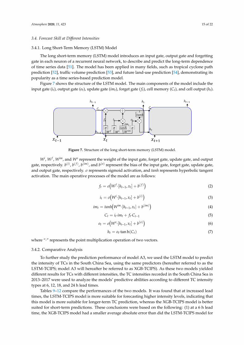
Figure 7 shows the structure of the LSTM model. The main components of the model include the input gate ( ), output gate ( ), update gate ( ), forget gate ( ), cell memory ( ), and cell output (ℎ ).

Figure 6. Scatter plots of the actual intensity and the intensities predicted by models A1, A2, and A3 at6, 12, 18, and 24 h lead times. Actual intensity values are shown along the abscissa axes and predictedintensity values along the ordinate axes.

Atmosphere 2020, 11, 423 15 of 22

3.4. Forecast Skill at Different Intensities

3.4.1. Long Short-Term Memory (LSTM) Model

The long short-term memory (LSTM) model introduces an input gate, output gate and forgettinggate in each neuron of a recurrent neural network, to describe and predict the long-term dependenceof time series data [51]. The model has been applied in many fields, such as tropical cyclone pathprediction [52], traffic volume prediction [53], and future land-use prediction [54], demonstrating itspopularity as a time series-based prediction model.

Figure 7 shows the structure of the LSTM model. The main components of the model include theinput gate (it), output gate (ot), update gate (imt), forget gate ( ft), cell memory (Ct), and cell output (ht).Atmosphere 2020, 10, x FOR PEER REVIEW 15 of 22

Figure 7. Structure of the long short-term memory (LSTM) model.

, , , and represent the weight of the input gate, forget gate, update gate, and output gate, respectively. ( ), ( ), ( ), and ( ) represent the bias of the input gate, forget gate, update gate, and output gate, respectively. represents sigmoid activation, and ℎ represents hyperbolic tangent activation. The main operative processes of the model are as follows: = ∙ ℎ , + ( ) (2) = ∙ ℎ , + ( ) (3) = ℎ ∙ ℎ , + ( ) (4) = ∙ + ∙ (5) = ∙ ℎ , + ( ) (6) ℎ = ∙ tanh( ) (7)

where “∙” represents the point multiplication operation of two vectors.

3.4.2. Comparative Analysis

To further study the prediction performance of model A3, we used the LSTM model to predict the intensity of TCs in the South China Sea, using the same predictors (hereafter referred to as the LSTM-TCIPS; model A3 will hereafter be referred to as XGB-TCIPS). As these two models yielded different results for TCs with different intensities, the TC intensities recorded in the South China Sea in 2013–2017 were used to analyze the models’ predictive abilities according to different TC intensity types at 6, 12, 18, and 24 h lead times.

Tables 9–12 compare the performances of the two models. It was found that at increased lead times, the LSTM-TCIPS model is more suitable for forecasting higher intensity levels, indicating that this model is more suitable for longer-term TC prediction, whereas the XGB-TCIPS model is better suited for short-term predictions. These conclusions were based on the following: (1) at a 6 h lead time, the XGB-TCIPS model had a smaller average absolute error than did the LSTM-TCIPS model for TCs of all intensity levels, and the XGB-TCIPS model was suitable for all intensity types. (2) At a 12 h lead time, the XGB-TCIPS model was more suitable for the prediction of tropical depressions, severe tropical storms, typhoons, and strong typhoons, whereas the LSTM-TCIPS model was better suited for the prediction of super typhoons. (3) At an 18 h lead time, the XGB-TCIPS model was better suited for the prediction of tropical depressions, severe tropical storms, typhoons, strong typhoons, and super typhoons, whereas LSTM-TCIPS was better suited for the prediction of tropical storms. (4) For a 24 h lead time, the XGB-TCIPS model was more suitable for the prediction of tropical depressions, typhoons, and strong typhoons, and the LSTM-TCIPS model was better suited for the prediction of tropical storms, severe tropical storms, and super typhoons.

Figure 7. Structure of the long short-term memory (LSTM) model.

Wi, W f , Wim, and Wo represent the weight of the input gate, forget gate, update gate, and outputgate, respectively. b(i), b( f ), b(im), and b(o) represent the bias of the input gate, forget gate, update gate,and output gate, respectively. σ represents sigmoid activation, and tanh represents hyperbolic tangentactivation. The main operative processes of the model are as follows:

ft = σ(W f·[ht−1, xt] + b( f )

)(2)

it = σ(Wi·[ht−1, xt] + b(i)

)(3)

imt = tanh(Wim·[ht−1, xt] + b(im)

)(4)

Ct = it·imt + ft·Ct−1 (5)

ot = σ(Wo·[ht−1, xt] + b(o)

)(6)

ht = ot·tan h(Ct) (7)

where “·” represents the point multiplication operation of two vectors.

3.4.2. Comparative Analysis

To further study the prediction performance of model A3, we used the LSTM model to predictthe intensity of TCs in the South China Sea, using the same predictors (hereafter referred to as theLSTM-TCIPS; model A3 will hereafter be referred to as XGB-TCIPS). As these two models yieldeddifferent results for TCs with different intensities, the TC intensities recorded in the South China Sea in2013–2017 were used to analyze the models’ predictive abilities according to different TC intensitytypes at 6, 12, 18, and 24 h lead times.

Tables 9–12 compare the performances of the two models. It was found that at increased leadtimes, the LSTM-TCIPS model is more suitable for forecasting higher intensity levels, indicating thatthis model is more suitable for longer-term TC prediction, whereas the XGB-TCIPS model is bettersuited for short-term predictions. These conclusions were based on the following: (1) at a 6 h leadtime, the XGB-TCIPS model had a smaller average absolute error than did the LSTM-TCIPS model for

Atmosphere 2020, 11, 423 16 of 22

TCs of all intensity levels, and the XGB-TCIPS model was suitable for all intensity types. (2) At a 12 hlead time, the XGB-TCIPS model was more suitable for the prediction of tropical depressions, severetropical storms, typhoons, and strong typhoons, whereas the LSTM-TCIPS model was better suited forthe prediction of super typhoons. (3) At an 18 h lead time, the XGB-TCIPS model was better suited forthe prediction of tropical depressions, severe tropical storms, typhoons, strong typhoons, and supertyphoons, whereas LSTM-TCIPS was better suited for the prediction of tropical storms. (4) For a24 h lead time, the XGB-TCIPS model was more suitable for the prediction of tropical depressions,typhoons, and strong typhoons, and the LSTM-TCIPS model was better suited for the prediction oftropical storms, severe tropical storms, and super typhoons.

Table 9. LSTM and XGBoost model errors for different tropical cyclone intensity levels at a 6 h lead time.

TypeLSTM XGBoost

MAE (m/s) NRMSE MAE (m/s) NRMSE

Tropical depression 1.56 3.10 1.45 2.9Tropical storm 2.07 4.05 1.89 4.21

Severe tropical storm 3.48 6.62 2.34 5.49Typhoon 6.91 12.19 2.99 5.87

Severe typhoon 12.23 20.49 2.74 5.36Super typhoon 19.77 32.73 13.91 24.6

Note: LSTM: long short-term memory; MAE: mean absolute error; NRMSE: normalized root mean square error.

Table 10. LSTM and XGBoost model errors for different tropical cyclone intensity levels at a 12 hlead time.

TypeLSTM XGBoost






Table 11. LSTM and XGBoost model errors for different tropical cyclone intensity levels at an 18 hlead time.

TypeLSTM XGBoost






Atmosphere 2020, 11, 423 17 of 22

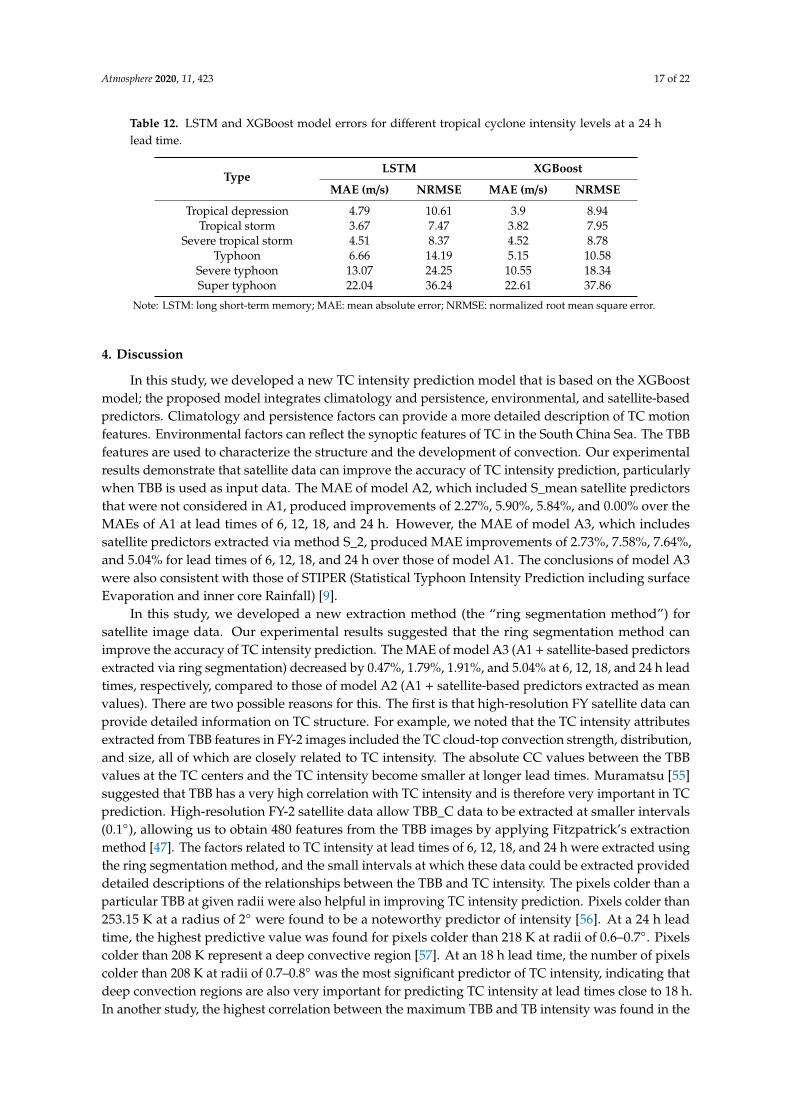
Table 12. LSTM and XGBoost model errors for different tropical cyclone intensity levels at a 24 hlead time.

TypeLSTM XGBoost






4. Discussion

In this study, we developed a new TC intensity prediction model that is based on the XGBoostmodel; the proposed model integrates climatology and persistence, environmental, and satellite-basedpredictors. Climatology and persistence factors can provide a more detailed description of TC motionfeatures. Environmental factors can reflect the synoptic features of TC in the South China Sea. The TBBfeatures are used to characterize the structure and the development of convection. Our experimentalresults demonstrate that satellite data can improve the accuracy of TC intensity prediction, particularlywhen TBB is used as input data. The MAE of model A2, which included S_mean satellite predictorsthat were not considered in A1, produced improvements of 2.27%, 5.90%, 5.84%, and 0.00% over theMAEs of A1 at lead times of 6, 12, 18, and 24 h. However, the MAE of model A3, which includessatellite predictors extracted via method S_2, produced MAE improvements of 2.73%, 7.58%, 7.64%,and 5.04% for lead times of 6, 12, 18, and 24 h over those of model A1. The conclusions of model A3were also consistent with those of STIPER (Statistical Typhoon Intensity Prediction including surfaceEvaporation and inner core Rainfall) [9].

In this study, we developed a new extraction method (the “ring segmentation method”) forsatellite image data. Our experimental results suggested that the ring segmentation method canimprove the accuracy of TC intensity prediction. The MAE of model A3 (A1 + satellite-based predictorsextracted via ring segmentation) decreased by 0.47%, 1.79%, 1.91%, and 5.04% at 6, 12, 18, and 24 h leadtimes, respectively, compared to those of model A2 (A1 + satellite-based predictors extracted as meanvalues). There are two possible reasons for this. The first is that high-resolution FY satellite data canprovide detailed information on TC structure. For example, we noted that the TC intensity attributesextracted from TBB features in FY-2 images included the TC cloud-top convection strength, distribution,and size, all of which are closely related to TC intensity. The absolute CC values between the TBBvalues at the TC centers and the TC intensity become smaller at longer lead times. Muramatsu [55]suggested that TBB has a very high correlation with TC intensity and is therefore very important in TCprediction. High-resolution FY-2 satellite data allow TBB_C data to be extracted at smaller intervals(0.1◦), allowing us to obtain 480 features from the TBB images by applying Fitzpatrick’s extractionmethod [47]. The factors related to TC intensity at lead times of 6, 12, 18, and 24 h were extracted usingthe ring segmentation method, and the small intervals at which these data could be extracted provideddetailed descriptions of the relationships between the TBB and TC intensity. The pixels colder than aparticular TBB at given radii were also helpful in improving TC intensity prediction. Pixels colder than253.15 K at a radius of 2◦ were found to be a noteworthy predictor of intensity [56]. At a 24 h leadtime, the highest predictive value was found for pixels colder than 218 K at radii of 0.6–0.7◦. Pixelscolder than 208 K represent a deep convective region [57]. At an 18 h lead time, the number of pixelscolder than 208 K at radii of 0.7–0.8◦ was the most significant predictor of TC intensity, indicating thatdeep convection regions are also very important for predicting TC intensity at lead times close to 18 h.In another study, the highest correlation between the maximum TBB and TB intensity was found in the

Atmosphere 2020, 11, 423 18 of 22

1.4◦ radial area at a 0–36 h lead time [45]. In this study, the highest correlation between TBB and TCintensity was found in the 1.1–1.5◦ radial area at a 6–12 h lead time. Because our extraction methodallowed us to employ high-resolution FY-2 satellite data, our results can be considered more precisethan those found in previous studies.

The second reason that the ring segmentation method led to better results is that the XGBoostmodel allows multi-predictor input. In this study, we assessed the response of the model to differentcombinations of input features related to TC intensity in the South China Sea, such as inner-coreconvection, climatology and persistence factors, and environmental factors. The resulting combinationof predictors obtained from the TBB features derived from the FY-2 satellite data, the best track datataken from the CMA-STI, and environmental information obtained from the ERA-Interim datasetwere then used to build the final model. Because the model primarily uses randomly selectedfeatures, each tree can be built from a random set of features rather than the overall set. Combiningall trees constructed in this manner led to the most accurate predictions. In this study, we usedapproximately 100 predictors that did not produce any serious over-fitting in the XGBoost model,because an appropriate scale was used to select the eta hyperparameters. However, we did identifyone limitation in our proposed model. Its errors when predicting the intensity of very strong storms inthe “severe typhoon” and “super typhoon” intensity categories were substantially large at lead times of6, 12, 18, 24 h. This limitation is likely attributable to the relatively low number of samples concerninghigh-intensity TC events, leading to larger model errors concerning these types of storms. Figure 8shows the frequencies of different TC intensities in the South China Sea from 2006 to 2012. Cyclonesin the severe typhoon and super typhoon categories have the lowest occurrence in the training data.Owing to the lack of training samples, the accuracy of the model, with regard to severe typhoons andsuper typhoons, is low.


samples concerning high-intensity TC events, leading to larger model errors concerning these types of storms. Figure 8 shows the frequencies of different TC intensities in the South China Sea from 2006 to 2012. Cyclones in the severe typhoon and super typhoon categories have the lowest occurrence in the training data. Owing to the lack of training samples, the accuracy of the model, with regard to severe typhoons and super typhoons, is low.

Figure 8. Frequencies of tropical cyclones of different intensities in the South China Sea from 2006 to 2012. TD: Tropical depression; TS: tropical storm; STS: severe tropical storm; TY: Typhoon; STY: Severe typhoon; SuperTY: Super typhoon.

The XGBoost method and the LSTM method can both predict TC intensity from a non-linear perspective. The XGBoost method essentially incorporates the XGBoost algorithm into the TC intensity prediction model, which improves the average absolute error of the existing TC intensity model predictions. The combination of feature selection and the spatio-temporal consideration of the LSTM model can also improve TC intensity predictions. The performance of each of the models seems to be dependent on lead time; the XGBoost model is best applied to the prediction of TC intensity at short lead times. At a 6 h lead time, the MAE and NRMSE values obtained using the XGBoost model were better than those of the LSTM model, for storms of all intensity levels. The LSTM model can sometimes provide better performance than the XGBoost model at longer lead times. At a 24 h lead time, the LSTM model is better suited for the prediction of tropical storms, severe tropical storms, and super typhoons than is the XGBoost model. However, the XGBoost method and the LSTM method may not fit the prediction of the TC intensity in the South China Sea at 72 h lead time. This limitation is likely attributable to the relatively low number of samples concerning TC events at 72 h lead time. The lack of sample is one of the bottlenecks for predicting TC intensity using non-linear method [58]. Overall, both models offer improved Fengyun-2 satellite data utilization over that of other models and represent promising advances in TC intensity prediction at 6, 12, 18, and 24 h lead times.

5. Conclusions

Using TBB features derived from FY-2 satellite data, best-track data derived from the CMA-STI, and environmental information taken from the ERA-Interim dataset as input data, we used the XGBoost model to simulate and predict the intensity of TCs in the South China Sea, at lead times of 6, 12, 18, and 24 h. We analyzed the influence of satellite data utilization and explored the most accurate parameter sets under three scenarios. The examined prediction models were built based on climatology and persistence predictors, environmental predictors, and satellite-based predictors. The traditional extraction method for satellite image data directly extracts average values from the images, but it cannot fully reflect the cloud-based characteristics. Based on existing research, this study employed a high-precision and maneuverable ring segmentation method for satellite-based predictor extraction and compared its performance to that of the conventional method. We trained the models using TC event data from 2006–2012 and verified the accuracy of their TC-intensity predictions using TC event data from 2013–2017. The results were as follows.

Figure 8. Frequencies of tropical cyclones of different intensities in the South China Sea from 2006 to2012. TD: Tropical depression; TS: tropical storm; STS: severe tropical storm; TY: Typhoon; STY: Severetyphoon; SuperTY: Super typhoon.

The XGBoost method and the LSTM method can both predict TC intensity from a non-linearperspective. The XGBoost method essentially incorporates the XGBoost algorithm into the TC intensityprediction model, which improves the average absolute error of the existing TC intensity modelpredictions. The combination of feature selection and the spatio-temporal consideration of the LSTMmodel can also improve TC intensity predictions. The performance of each of the models seems tobe dependent on lead time; the XGBoost model is best applied to the prediction of TC intensity atshort lead times. At a 6 h lead time, the MAE and NRMSE values obtained using the XGBoost modelwere better than those of the LSTM model, for storms of all intensity levels. The LSTM model cansometimes provide better performance than the XGBoost model at longer lead times. At a 24 h leadtime, the LSTM model is better suited for the prediction of tropical storms, severe tropical storms,and super typhoons than is the XGBoost model. However, the XGBoost method and the LSTM methodmay not fit the prediction of the TC intensity in the South China Sea at 72 h lead time. This limitation is

Atmosphere 2020, 11, 423 19 of 22

likely attributable to the relatively low number of samples concerning TC events at 72 h lead time.The lack of sample is one of the bottlenecks for predicting TC intensity using non-linear method [58].Overall, both models offer improved Fengyun-2 satellite data utilization over that of other models andrepresent promising advances in TC intensity prediction at 6, 12, 18, and 24 h lead times.

5. Conclusions

Using TBB features derived from FY-2 satellite data, best-track data derived from the CMA-STI,and environmental information taken from the ERA-Interim dataset as input data, we used the XGBoostmodel to simulate and predict the intensity of TCs in the South China Sea, at lead times of 6, 12,18, and 24 h. We analyzed the influence of satellite data utilization and explored the most accurateparameter sets under three scenarios. The examined prediction models were built based on climatologyand persistence predictors, environmental predictors, and satellite-based predictors. The traditionalextraction method for satellite image data directly extracts average values from the images, but itcannot fully reflect the cloud-based characteristics. Based on existing research, this study employed ahigh-precision and maneuverable ring segmentation method for satellite-based predictor extractionand compared its performance to that of the conventional method. We trained the models using TCevent data from 2006–2012 and verified the accuracy of their TC-intensity predictions using TC eventdata from 2013–2017. The results were as follows.

(1) The Fengyun-2 satellite data can be used to increase the accuracy of TC intensity forecasts forthe South China Sea at 6, 12, 18, and 24 h lead times. We analyzed the influence of satellite data onthe accuracy of TC intensity forecasts under three models; the MAEs of models A2 and A3, whichemployed satellite-based prediction factors, were smaller than the MAE of model A1 at 6, 12, 18,and 24 h lead times.

(2) The ring segmentation method was found to be a suitable extraction method for satellitedata. Compared with that of model A2 (which considered satellite predictors extracted as averages),the MAE of model A3 decreased by 0.47%, 1.79%, 1.91%, and 5.04% at 6, 12, 18, and 24 h lead times,respectively. The relative biases of model A3 were 8.62%, 12.57%, 16.48%, and 19.04% at 6, 12, 18,and 24 h lead times, respectively; the R squares of model A3 were 0.91, 0.82, 0.73, 0.63 at 6, 12, 18,and 24 h lead times, respectively; the NRMSEs of model A3 were 5.28, 8.19, 9.42, and 10.51 at 6, 12, 18,and 24 h lead times, respectively.

(3) The TC intensity forecast results of the LSTM and XGBoost models for the South China Seafrom 2013 to 2017 were analyzed. The XGBoost model was found to be more stable and better suitedfor 6 h TC intensity predictions than the LSTM model.

Overall, these results suggest that the proposed XGBoost model and extraction method can beused to accurately estimate TC intensities in the South China Sea, using satellite data and optimizedparameter sets. The MAE, NRMSE, and CC results used to compare the three different modelingapproaches further suggest that satellite data might be the most important type of predictor and thatthe ring segmentation method might be the best available extraction method for such satellite data.

Author Contributions: Q.J. contributed to the development of the original idea for the study and wrote themajority of the paper. X.F. contributed to the manuscript structure. J.L. contributed to the data analysis. Z.X.analyzed and processed the TC activity. H.J. helped with field work, discussion, and revisions. All authors haveread and agreed to the published version of the manuscript.

Funding: This research was supported by the Strategic Priority Research Program of the Chinese Academy ofSciences, grant number XDA19080101, the National Key Research and Development Program of China, grantnumber 2016YFB0501502 and 2016YFB0501503, and the Key Research Program of the Chinese Academy of Sciences,grant number KFZD-SW-317.

Acknowledgments: All the data used in this study are available as follows: (1) The 2006–2017 South China SeaTC datasets were downloaded from the CMA-STI Best Track Dataset of TCs over the Western North Pacific (http://www.typhoon.gov.cn/). (2) The environmental datasets were produced by the ECMWF Re-Analysis (ERA-Interim)dataset. This dataset provides assimilation analysis data four times daily at 00:00, 06:00, 12:00, and 18:00, with aspatial resolution of 1◦ × 1◦. (3) The FY-2 data obtained for this study were downloaded from the National SatelliteMeteorological Center FengYun Satellite Data Center (http://satellite.nsmc.org.cn/PortalSite/Data/FileShow.aspx).



http://satellite.nsmc.org.cn/PortalSite/Data/FileShow.aspx

Atmosphere 2020, 11, 423 20 of 22

The selected satellite product was the TBB, which represents the most primitive observational data for cloudformation and enhancement display. The authors thank the four anonymous reviewers for their valuable comments.

Conflicts of Interest: The authors declare no conflict of interest.

References

1. Demaria, M.; Sampson, C.R.; Knaff, J.A.; Musgrave, K.D. Is Tropical Cyclone Intensity Guidance Improving?Bull. Am. Meteorol. Soc. 2014, 95, 387–398. [CrossRef]

2. Kovordányi, R.; Roy, C. Cyclone track forecasting based on satellite images using artificial neural networks.ISPRS J. Photogramm. Remote. Sens. 2009, 64, 513–521. [CrossRef]

3. Ichikawa, H.; Masunaga, H.; Tsushima, Y.; Kanzawa, H. Analysis of Cloud Properties Associated withTropical Convection in Climate Models and Satellite Data. J. Meteorol. Soc. Jpn. 2012, 90, 629–646. [CrossRef]

4. Mueller, K.J.; Demaria, M.; Knaff, J.; Kossin, J.P.; Haar, T.V. Objective Estimation of Tropical Cyclone WindStructure from Infrared Satellite Data. Weather Forecast. 2006, 21, 990–1005. [CrossRef]

5. Ghosh, T.; Krishnamurti, T.N. Improvements in Hurricane Intensity Forecasts from a MultimodelSuperensemble Utilizing a Generalized Neural Network Technique. Weather Forecast. 2018, 33, 873–885.[CrossRef]

6. Roy, C.; Kovordányi, R. Tropical cyclone track forecasting techniques—A review. Atmos. Res. 2012, 104–105,40–69. [CrossRef]

7. DeMaria, M.; Mainelli, M.; Shay, L.K.; Knaff, J.A.; Kaplan, J. Further improvements to the Statistical HurricaneIntensity Prediction Scheme (SHIPS). Weather Forecast. 2005, 20, 531–543. [CrossRef]

8. Knaff, J.A.; Sampson, C.R.; Demaria, M. An Operational Statistical Typhoon Intensity Prediction Scheme forthe Western North Pacific. Weather Forecast. 2005, 20, 688–699. [CrossRef]

9. Gao, S.; Chiu, L.S. Development of Statistical Typhoon Intensity Prediction: Application to Satellite-ObservedSurface Evaporation and Rain Rate (STIPER). Weather Forecast. 2012, 27, 240–250. [CrossRef]

10. Chaudhuri, S.; Dutta, D.; Goswami, S.; Middey, A. Intensity forecast of tropical cyclones over North IndianOcean using multilayer perceptron model: Skill and performance verification. Nat. Hazards 2013, 65, 97–113.[CrossRef]

11. Chaudhuri, S.; Dutta, D.; Goswami, S.; Middey, A. Track and intensity forecast of tropical cyclones over theNorth Indian Ocean with multilayer feed forward neural nets. Meteorol. Appl. 2015, 22, 563–575. [CrossRef]

12. Huang, Y.; Jin, L. A prediction scheme with genetic neural network and Isomap algorithm for tropical cycloneintensity change over western North Pacific. Theor. Appl. Clim. 2013, 121, 143–152. [CrossRef]

13. Gao, S.; Zhang, W.; Liu, J.; Lin, I.-I.; Chiu, L.S.; Cao, K. Improvements in Typhoon Intensity ChangeClassification by Incorporating an Ocean Coupling Potential Intensity Index into Decision Trees. WeatherForecast. 2016, 31, 95–106. [CrossRef]

14. Asif, A.; Dawood, M.; Jan, B.; Khurshid, J.; DeMaria, M.; Minhas, F.U.A.A. PHURIE: Hurricane intensityestimation from infrared satellite imagery using machine learning. Neural Comput. Appl. 2018. [CrossRef]

15. Wang, Z. What is the Key Feature of Convection Leading up to Tropical Cyclone Formation? J. Atmos. Sci.2018, 75, 1609–1629. [CrossRef]

16. Fetanat Fard Haghighi, G. Tropical Cyclone Intensity Estimation Using Temporal and Spatial Features fromSatellite Data. Ph.D. Thesis, North Carolina Agricultural and Technical State University, Greensboro, NC,USA, 2013.

17. Zhang, W.; Gao, S.; Chen, B.; Cao, K. The application of decision tree to intensity change classification oftropical cyclones in western North Pacific. Geophys. Res. Lett. 2013, 40, 1883–1887. [CrossRef]

18. Chen, T.; Guestrin, C. XGBoost: A Scalable Tree Boosting System. In Proceedings of the Acm Sigkdd InternationalConference on Knowledge Discovery & Data Mining, San Francisco, CA, USA, 13–17 August 2016.

19. Ren, X.D.; Guo, H.N.; Li, S.H.; Wang, S.L.; Li, J.H. A Novel Image Classification Method with CNN-XGBoostModel. In Digital Forensics and Watermarking; Kraetzer, C., Shi, Y.Q., Dittmann, J., Kim, H.J., Eds.; Springer:Berlin/Heidelberg, Germany, 2017; Volume 10431, pp. 378–390.

http://dx.doi.org/10.1175/BAMS-D-12-00240.1

http://dx.doi.org/10.1016/j.isprsjprs.2009.03.002

http://dx.doi.org/10.2151/jmsj.2012-504

http://dx.doi.org/10.1175/WAF955.1

http://dx.doi.org/10.1175/WAF-D-17-0006.1

http://dx.doi.org/10.1016/j.atmosres.2011.09.012




http://dx.doi.org/10.1007/s11069-012-0346-7

http://dx.doi.org/10.1002/met.1488

http://dx.doi.org/10.1007/s00703-013-0263-7


http://dx.doi.org/10.1007/s00521-018-3874-6

http://dx.doi.org/10.1175/JAS-D-17-0131.1

http://dx.doi.org/10.1002/grl.50280

Atmosphere 2020, 11, 423 21 of 22

20. Chittaragi, N.B.; Koolagudi, S.G. Acoustic Features based Word Level Dialect Classification using SVM andEnsemble Methods. In Proceedings of the 2017 Tenth International Conference on Contemporary Computing,NOIDA, India, 10–12 August 2017; Aluru, S., Kalyanaraman, A., Ucar, B., Kothapalli, K., Halappanavar, M.,Madduri, K., Govindaraju, M., Xia, Y., Prasad, S., Barnas, M., et al., Eds.; IEEE: New York, NY, USA, 2017;pp. 178–183.

21. Tahmassebi, A.; Wengert, G.J.; Helbich, T.H.; Bago-Horvath, Z.; Alaei, S.; Bartsch, R.; Dubsky, P.; Balizen, P.;Clausen, P.; Kapetas, P.; et al. Impact of Machine Learning With Multiparametric Magnetic ResonanceImaging of the Breast for Early Prediction of Response to Neoadjuvant Chemotherapy and Survival Outcomesin Breast Cancer Patients. Investig. Radiol. 2019, 54, 110–117. [CrossRef]

22. Jin, Q.; Fan, X.; Liu, J.; Xue, Z.; Jian, H. Using eXtreme Gradient BOOSTing to Predict Changes in TropicalCyclone Intensity over the Western North Pacific. Atmosphere 2019, 10, 341. [CrossRef]

23. Yang, R.; Tang, J.; Sun, D. Association Rule Data Mining Applications for Atlantic Tropical Cyclone IntensityChanges. Weather Forecast. 2011, 26, 337–353. [CrossRef]

24. Yang, R.; Tang, J.; Kafatos, M. Improved associated conditions in rapid intensifications of tropical cyclones.Geophys. Res. Lett. 2007, 34. [CrossRef]

25. Ming, Y.; Wei, Z.; Hui, Y.; Lu, X.; Feng, J.; Fan, Y.; Zhu, Y.; Chen, D. An Overview of the China MeteorologicalAdministration Tropical Cyclone Database. J. Atmospheric Ocean. Technol. 2014, 31, 287–301.

26. Kalnay, E.; Kanamitsu, M.; Kistler, R.; Collins, W.; Deaven, D.; Gandin, L.; Iredell, M.; Saha, S.; White, G.;Woollen, J.; et al. The NCEP/NCAR 40-year reanalysis project. Bull. Am. Meteorol. Soc. 1996, 77, 437–472.[CrossRef]

27. Huang, X.; Guan, Z.; He, L.; Huang, Y.; Zhao, H. A PNN prediction scheme for local tropical cyclone intensityover the South China Sea. Nat. Hazards 2016, 81, 1249–1267. [CrossRef]

28. Longsheng, L.; Xinyan, L.; Shuanzhu, G. Overview of typhoon activities over western North Pacific and theSouth China Sea. J. Mar. Meteorol. 2019, 39, 1–12.

29. Loy, K.C.; Sinha, P.C.; Liew, J.; Tangang, F.; Husain, M.L. Modeling storm surges associated with supertyphoon durian in South China Sea. Nat. Hazards 2014, 70, 23–37. [CrossRef]

30. Berrisford, P.; Dee, D.P.; Poli, P.; Brugge, R.; Mark, F.; Manuel, F.; Kållberg, P.W.; Kobayashi, S.; Uppala, S.;Adrian, S. The ERA-Interim Archive Version 2.0; ECMWF: Shinfield Park, Reading, UK, 2011.

31. Zhu, P.J.; Zheng, Y.G.; Zheng, P.Q. Asymmetric Distribution of Convection Associated with Tropical CyclonesMaking Landfall on the East China Coast. J. Trop. Meteorol. 2012, 18, 436–444.

32. Wang, X.; Guo, Q.; Wen, R. Inner dynamic mechanism analysis for tropical cyclone rapid intensificationbased on FY-2 cloud motion. J. Infrared Millim. Waves 2018, 37, 790–798. [CrossRef]

33. Zhou, Y.S.; Wu, T.Y. Composite analysis of precipitation intensity and distribution characteristics of westerntrack landfall typhoons over China under strong and weak monsoon conditions. Atmos. Res. 2019, 225,131–143. [CrossRef]

34. FENGYUN Satellite Data Center. Available online: http://satellite.nsmc.org.cn/PortalSite/Data/Satellite.aspx(accessed on 24 June 2019).

35. Aoki, T. A Statistical Prediction of the Tropical Cyclone Position Based on Persistence Climatological Factorin the Western North Pacific (the PC method). Geophs. Mag. 1979, 38, 17–27.

36. Baik, J.J.; Paek, J.S. A neural network model for predicting typhoon intensity. J. Meteorol. Soc. Jpn. 2000, 78,857–869. [CrossRef]

37. Dongqing, Z. Research on Tropical Cyclone in the South China Sea Forecast; Nanjing Normal University: Nanjing,China, 2012.

38. Kalnay, E. Atmospheric Modeling, Data Assimilation and Predictability; Cambridge University Press: Cambridge,UK, 2003.

39. Demaria, M.; Kaplan, J. Sea Surface Temperature and the Maximum Intensity of Atlantic Tropical Cyclones.J. Climate 1994, 7, 1324–1334. [CrossRef]

40. Holland, G.J. The Maximum Potential Intensity of Tropical Cyclones. J. Atmos. Sci. 1997, 54, 2519–2541.[CrossRef]

41. Miller, B.I. O the Maximum Intensity of Hurricanes. J. Atmos. Sci. 1958, 15, 184–195. [CrossRef]42. Merrill, R.T. An experiment in the statistical prediction of tropical cyclone intensity change. In Proceedings

of the 17th Conference on Hurricanes and Tropical Meteorology, Miami, FL, USA, 7–10 April 1987.

http://dx.doi.org/10.1097/RLI.0000000000000518

http://dx.doi.org/10.3390/atmos10060341


http://dx.doi.org/10.1029/2007GL031241

http://dx.doi.org/10.1175/1520-0477(1996)077<0437:TNYRP>2.0.CO;2

http://dx.doi.org/10.1007/s11069-015-2132-9

http://dx.doi.org/10.1007/s11069-010-9674-7

http://dx.doi.org/10.11972/j.issn.1001-9014.2018.06.025

http://dx.doi.org/10.1016/j.atmosres.2019.03.037

http://satellite.nsmc.org.cn/PortalSite/Data/Satellite.aspx

http://dx.doi.org/10.2151/jmsj1965.78.6_857

http://dx.doi.org/10.1175/1520-0442(1994)007<1324:SSTATM>2.0.CO;2

http://dx.doi.org/10.1175/1520-0469(1997)054<2519:TMPIOT>2.0.CO;2

http://dx.doi.org/10.1175/1520-0469(1958)015<0184:OTMIOH>2.0.CO;2

Atmosphere 2020, 11, 423 22 of 22

43. Wikle, C.K. Atmospheric Modeling, Data Assimilation, and Predictability. Technometrics 2002, 47, 521.[CrossRef]

44. Geng, H.; Sun, J.; Wei, Z.; Chao, H. Study on Index Model of Tropical Cyclone Intensity Change Basedon Projection Pursuit and Evolution Strategy. In Proceedings of the 2015 IEEE Symposium Series onComputational Intelligence (SSCI), Cape Town, South Africa, 7–10 December 2015.

45. Chen, P.Y.; Duan, Y.H.; Yu, H.; Hu, C.M. Application of equivalent black body temperature in the forecast oftropical cyclone intensity. Acta Meteorol. Sin. 2007, 21, 465–475.

46. Steranka, J.; Rodgers, E.B.; Gentry, R.C. The Relationship between Satellite Measured Convective Bursts andTropical Cyclone Intensification. Mon. Weather. Rev. 1986, 114, 1539. [CrossRef]

47. Fitzpatrick, P.J. Understanding and forecasting tropical cyclone intensity change with the Typhoon IntensityPrediction Scheme (TIPS). Weather Forecast. 1997, 12, 826–846. [CrossRef]

48. Weatherford, C.L.; Gray, W.M. Typhoon Structure as Revealed by Aircraft Reconnaissance. Part I: DataAnalysis and Climatology. Mon. Weather Rev. 1988, 116, 1032–1043. [CrossRef]

49. Mundell, D.B. Prediction of Tropical Cyclone Rapid Intensification Intensification; Colorado State University: FortCollins, CO, USA, 1990.

50. Olander, T.L.; Velden, C.S. The Advanced Dvorak Technique: Continued Development of an ObjectiveScheme to Estimate Tropical Cyclone Intensity Using Geostationary Infrared Satellite Imagery. WeatherForecast. 2007, 22, 287–298. [CrossRef]

51. Hochreiter, S.; Schmidhuber, J. Long Short-Term Memory. Neural Comput. 1997, 9, 1735–1780. [CrossRef]52. Gao, S.; Zhao, P.; Pan, B.; Yaru, L.I.; Zhou, M.; Jiangling, X.U.; Zhong, S.; Shi, Z. A nowcasting model for the

prediction of typhoon tracks based on a long short term memory neural network. Acta Oceanol. Sin. 2018, 37,8–12. [CrossRef]

53. Ma, X.L.; Tao, Z.M.; Wang, Y.H.; Yu, H.Y.; Wang, Y.P. Long short-term memory neural network for trafficspeed prediction using remote microwave sensor data. Transp. Res. Pt. C-Emerg. Technol. 2015, 54, 187–197.[CrossRef]

54. Kong, Y.L.; Huang, Q.; Wang, C.; Chen, J.; Chen, J.; He, D. Long Short-Term Memory Neural Networks forOnline Disturbance Detection in Satellite Image Time Series. Remote Sens. 2018, 10, 452. [CrossRef]

55. Muramatsu, T. Diurnal Variations of Satellite-Measured TBB Areal Distribution and Eye Diameter of MatureTyphoons. J. Meteorol. Soc. Jpn. 2007, 61, 77–90. [CrossRef]

56. DeMaria, M.; Zehr, R.M.; Kossin, J.P.; Knaff, J.A. The use of GOES imagery in statistical hurricane intensityprediction. In Proceedings of the 25th Conference on Hurricanes and Tropical Meteorology, San Diego, CA,USA, 29 April–3 May 2002; pp. 120–121.

57. Ruan, Z.X.; Wu, Q.Y. Precipitation, Convective Clouds, and Their Connections with Tropical Cyclone Intensityand Intensity Change. Geophys. Res. Lett. 2018, 45, 1098–1105. [CrossRef]

58. Pradhan, R.; Aygun, R.; Maskey, M.; Ramachandran, R.; Cecil, D. Tropical Cyclone Intensity EstimationUsing a Deep Convolutional Neural Network. IEEE Trans. Image Process. 2018, 27, 692–702. [CrossRef]

© 2020 by the authors. Licensee MDPI, Basel, Switzerland. This article is an open accessarticle distributed under the terms and conditions of the Creative Commons Attribution(CC BY) license (http://creativecommons.org/licenses/by/4.0/).

http://dx.doi.org/10.1198/tech.2005.s326

http://dx.doi.org/10.1175/1520-0493(1986)114<1539:TRBSMC>2.0.CO;2

http://dx.doi.org/10.1175/1520-0434(1997)012<0826:UAFTCI>2.0.CO;2

http://dx.doi.org/10.1175/1520-0493(1988)116<1032:TSARBA>2.0.CO;2


http://dx.doi.org/10.1162/neco.1997.9.8.1735

http://dx.doi.org/10.1007/s13131-018-1219-z

http://dx.doi.org/10.1016/j.trc.2015.03.014

http://dx.doi.org/10.3390/rs10030452

http://dx.doi.org/10.2151/jmsj1965.61.1_77

http://dx.doi.org/10.1002/2017GL076611

http://dx.doi.org/10.1109/TIP.2017.2766358

http://creativecommons.org/

http://creativecommons.org/licenses/by/4.0/.

estimating tropical cyclone intensity in the south china

Documents