estimating toll road demand & revenue--trb, 2006
TRANSCRIPT

8/3/2019 Estimating Toll Road Demand & Revenue--TRB, 2006
http://slidepdf.com/reader/full/estimating-toll-road-demand-revenue-trb-2006 1/113
NATIONAL
COOPERATIVE
HIGHWAY RESEARCH
PROGRAMNCHRPSYNTHESIS 364
Estimating Toll Road
Demand and Revenue
A Synthesis of Highway Practice

8/3/2019 Estimating Toll Road Demand & Revenue--TRB, 2006
http://slidepdf.com/reader/full/estimating-toll-road-demand-revenue-trb-2006 2/113
TRANSPORTATION RESEARCH BOARD 2007 EXECUTIVE COMMITTEE*
OFFICERS
Chair: Linda S. Watson, CEO, LYNX–Central Florida Regional Transportation Authority, Orlando
Vice Chair: Carol A. Murray, Commissioner, New Hampshire DOT, Concord
Executive Director: Robert E. Skinner, Jr., Transportation Research Board
MEMBERS
J. BARRY BARKER, Executive Director, Transit Authority of River City, Louisville, KY
MICHAEL W. BEHRENS, Executive Director, Texas DOT, Austin
ALLEN D. BIEHLER, Secretary, Pennsylvania DOT, Harrisburg
JOHN D. BOWE, President, Americas Region, APL Limited, Oakland, CA
LARRY L. BROWN, SR., Executive Director, Mississippi DOT, Jackson
DEBORAH H. BUTLER, Vice President, Customer Service, Norfolk Southern Corporation and Subsidiaries, Atlanta, GA
ANNE P. CANBY, President, Surface Transportation Policy Partnership, Washington, DC
NICHOLAS J. GARBER, Henry L. Kinnier Professor, Department of Civil Engineering, University of Virginia, Charlottesville
ANGELA GITTENS, Vice President, Airport Business Services, HNTB Corporation, Miami, FL
SUSAN HANSON, Landry University Professor of Geography, Graduate School of Geography, Clark University, Worcester, MA
ADIB K. KANAFANI, Cahill Professor of Civil Engineering, University of California, Berkeley
HAROLD E. LINNENKOHL, Commissioner, Georgia DOT, Atlanta
MICHAEL D. MEYER, Professor, School of Civil and Environmental Engineering, Georgia Institute of Technology, Atlanta
DEBRA L. MILLER, Secretary, Kansas DOT, TopekaMICHAEL R. MORRIS, Director of Transportation, North Central Texas Council of Governments, Arlington
JOHN R. NJORD, Executive Director, Utah DOT, Salt Lake City
PETE K. RAHN, Director, Missouri DOT, Jefferson City
SANDRA ROSENBLOOM, Professor of Planning, University of Arizona, Tucson
TRACY L. ROSSER, Vice President, Corporate Traffic, Wal-Mart Stores, Inc., Bentonville, AR
ROSA CLAUSELL ROUNTREE, Executive Director, Georgia State Road and Tollway Authority, Atlanta
HENRY G. (GERRY) SCHWARTZ, JR., Senior Professor, Washington University, St. Louis, MO
C. MICHAEL WALTON, Ernest H. Cockrell Centennial Chair in Engineering, University of Texas, Austin
STEVE WILLIAMS, Chairman and CEO, Maverick Transportation, Inc., Little Rock, AR
EX OFFICIO MEMBERS
THAD ALLEN (Adm., U.S. Coast Guard), Commandant, U.S. Coast Guard, Washington, DC
THOMAS J. BARRETT (Vice Adm., U.S. Coast Guard, ret.), Pipeline and Hazardous Materials Safety Administrator, U.S.DOT
MARION C. BLAKEY, Federal Aviation Administrator, U.S.DOT JOSEPH H. BOARDMAN, Federal Railroad Administrator, U.S.DOT
JOHN A. BOBO, JR., Acting Administrator, Research and Innovative Technology Administration, U.S.DOT
REBECCA M. BREWSTER, President and COO, American Transportation Research Institute, Smyrna, GA
GEORGE BUGLIARELLO, Chancellor, Polytechnic University of New York, Brooklyn, and Foreign Secretary, National Academy
of Engineering, Washington, DC
J. RICHARD CAPKA, Federal Highway Administrator, U.S.DOT
SEAN T. CONNAUGHTON, Maritime Administrator, U.S.DOT
EDWARD R. HAMBERGER, President and CEO, Association of American Railroads, Washington, DC
JOHN H. HILL, Federal Motor Carrier Safety Administrator, U.S.DOT
JOHN C. HORSLEY, Executive Director, American Association of State Highway and Transportation Officials, Washington, DC
J. EDWARD JOHNSON, Director, Applied Science Directorate, National Aeronautics and Space Administration, John C. Stennis
Space Center, MS
WILLIAM W. MILLAR, President, American Public Transportation Association, Washington, DC
NICOLE R. NASON, National Highway Traffic Safety Administrator, U.S.DOT
JEFFREY N. SHANE, Under Secretary for Policy, U.S.DOT
JAMES S. SIMPSON, Federal Transit Administrator, U.S.DOT
CARL A. STROCK (Lt. Gen., U.S. Army), Chief of Engineers and Commanding General, U.S. Army Corps of Engineers, Washington, DC
*Membership as of January 2007.

8/3/2019 Estimating Toll Road Demand & Revenue--TRB, 2006
http://slidepdf.com/reader/full/estimating-toll-road-demand-revenue-trb-2006 3/113
TRANSPORTATION RESEARCH BOARD
WASHINGTON, D.C.
2006
www.TRB.org
NAT IONAL COOPERAT IVE H IGHWAY RESEARCH PROGRAM
NCHRP SYNTHESIS 364
Research Sponsored by the American Association of State Highway and Transportation Officials
in Cooperation with the Federal Highway Administration
SUBJECT AREAS
Planning and Administration
Estimating Toll Road Demand and Revenue
A Synthesis of Highway Practice
CONSULTANTS
DAVID KRIGER
SUZETTE SHIU
and
SASHA NAYLOR
iTRANS Consulting
Richmond Hill, ON, Canada

8/3/2019 Estimating Toll Road Demand & Revenue--TRB, 2006
http://slidepdf.com/reader/full/estimating-toll-road-demand-revenue-trb-2006 4/113
NATIONAL COOPERATIVE HIGHWAY RESEARCH PROGRAM
Systematic, well-designed research provides the most effective
approach to the solution of many problems facing highway
administrators and engineers. Often, highway problems are of local
interest and can best be studied by highway departments
individually or in cooperation with their state universities and
others. However, the accelerating growth of highway transportation
develops increasingly complex problems of wide interest to
highway authorities. These problems are best studied through a
coordinated program of cooperative research.
In recognition of these needs, the highway administrators of the
American Association of State Highway and Transportation
Officials initiated in 1962 an objective national highway research
program employing modern scientific techniques. This program is
supported on a continuing basis by funds from participating
member states of the Association and it receives the full cooperation
and support of the Federal Highway Administration, United States
Department of Transportation.
The Transportation Research Board of the National Academies
was requested by the Association to administer the research
program because of the Board’s recognized objectivity and
understanding of modern research practices. The Board is uniquely
suited for this purpose as it maintains an extensive committee
structure from which authorities on any highway transportation
subject may be drawn; it possesses avenues of communications and
cooperation with federal, state, and local governmental agencies,
universities, and industry; its relationship to the National Research
Council is an insurance of objectivity; it maintains a full-time
research correlation staff of specialists in highway transportation
matters to bring the findings of research directly to those who are in
a position to use them.
The program is developed on the basis of research needs
identified by chief administrators of the highway and transportation
departments and by committees of AASHTO. Each year, specific
areas of research needs to be included in the program are proposed
to the National Research Council and the Board by the American
Association of State Highway and Transportation Officials.
Research projects to fulfill these needs are defined by the Board, and
qualified research agencies are selected from those that have
submitted proposals. Administration and surveillance of research
contracts are the responsibilities of the National Research Council
and the Transportation Research Board.
The needs for highway research are many, and the National
Cooperative Highway Research Program can make significant
contributions to the solution of highway transportation problems of
mutual concern to many responsible groups. The program,
however, is intended to complement rather than to substitute for or
duplicate other highway research programs.
Published reports of the
NATIONAL COOPERATIVE HIGHWAY RESEARCH PROGRAM
are available from:
Transportation Research Board
Business Office
500 Fifth Street, NW
Washington, DC 20001
and can be ordered through the Internet at:
http://www.national-academies.org/trb/bookstore
Printed in the United States of America
NCHRP SYNTHESIS 364
Price $35.00
Project 20-5 (Topic 36-11)
ISSN 0547-5570
ISBN 978-0-3090-9776-5
Library of Congress Control No. 2006935402
© 2006 Transportation Research Board
COPYRIGHT PERMISSION
Authors herein are responsible for the authenticity of their materials and for
obtaining written permissions from publishers or persons who own the
copyright to any previously published or copyrighted material used herein.
Cooperative Research Programs (CRP) grants permission to reproduce
material in this publication for classroom and not-for-profit purposes.
Permission is given with the understanding that none of the material will be
used to imply TRB, AASHTO, FAA, FHWA, FMCSA, FTA, or Transit
Development Corporation endorsement of a particular product, method, or
practice. It is expected that those reproducing the material in this document
for educational and not-for-profit uses will give appropriate acknowledgment
of the source of any reprinted or reproduced material. For other uses of the
material, request permission from CRP.
NOTICE
The project that is the subject of this report was a part of the National
Cooperative Highway Research Program conducted by the Transportation
Research Board with the approval of the Governing Board of the National
Research Council. Such approval reflects the Governing Board’s judgment that
the program concerned is of national importance and appropriate with respect
to both the purposes and resources of the National Research Council.
The members of the technical committee selected to monitor this project and
to review this report were chosen for recognized scholarly competence and
with due consideration for the balance of disciplines appropriate to the project.
The opinions and conclusions expressed or implied are those of the research
agency that performed the research, and, while they have been accepted asappropriate by the technical committee, they are not necessarily those of the
Transportation Research Board, the National Research Council, the American
Association of State Highway and Transportation Officials, or the Federal
Highway Administration, U.S. Department of Transportation.
Each report is reviewed and accepted for publication by the technical
committee according to procedures established and monitored by the
Transportation Research Board Executive Committee and the Governing
Board of the National Research Council.
NOTE: The Transportation Research Board of the National Academies, theNational Research Council, the Federal Highway Administration, the AmericanAssociation of State Highway and Transportation Officials, and the individualstates participating in the National Cooperative Highway Research Program donot endorse products or manufacturers. Trade or manufacturers’ names appearherein solely because they are considered essential to the object of this report.

8/3/2019 Estimating Toll Road Demand & Revenue--TRB, 2006
http://slidepdf.com/reader/full/estimating-toll-road-demand-revenue-trb-2006 5/113
The National Academy of Sciences is a private, nonprofit, self-perpetuating society of distinguished schol-
ars engaged in scientific and engineering research, dedicated to the furtherance of science and technology
and to their use for the general welfare. On the authority of the charter granted to it by the Congress in
1863, the Academy has a mandate that requires it to advise the federal government on scientific and techni-
cal matters. Dr. Ralph J. Cicerone is president of the National Academy of Sciences.
The National Academy of Engineering was established in 1964, under the charter of the National Acad-
emy of Sciences, as a parallel organization of outstanding engineers. It is autonomous in its administration
and in the selection of its members, sharing with the National Academy of Sciences the responsibility for
advising the federal government. The National Academy of Engineering also sponsors engineering programs
aimed at meeting national needs, encourages education and research, and recognizes the superior achieve-
ments of engineers. Dr. William A. Wulf is president of the National Academy of Engineering.
The Institute of Medicine was established in 1970 by the National Academy of Sciences to secure theservices of eminent members of appropriate professions in the examination of policy matters pertaining
to the health of the public. The Institute acts under the responsibility given to the National Academy of
Sciences by its congressional charter to be an adviser to the federal government and, on its own initiative,
to identify issues of medical care, research, and education. Dr. Harvey V. Fineberg is president of the
Institute of Medicine.
The National Research Council was organized by the National Academy of Sciences in 1916 to associate
the broad community of science and technology with the Academy’s purposes of furthering knowledge and
advising the federal government. Functioning in accordance with general policies determined by the Acad-
emy, the Council has become the principal operating agency of both the National Academy of Sciences
and the National Academy of Engineering in providing services to the government, the public, and the
scientific and engineering communities. The Council is administered jointly by both the Academies and
the Institute of Medicine. Dr. Ralph J. Cicerone and Dr. William A. Wulf are chair and vice chair,
respectively, of the National Research Council.The Transportation Research Board is a division of the National Research Council, which serves the
National Academy of Sciences and the National Academy of Engineering. The Board’s mission is to promote
innovation and progress in transportation through research. In an objective and interdisciplinary setting,
the Board facilitates the sharing of information on transportation practice and policy by researchers and
practitioners; stimulates research and offers research management services that promote technical
excellence; provides expert advice on transportation policy and programs; and disseminates research
results broadly and encourages their implementation. The Board’s varied activities annually engage more
than 5,000 engineers, scientists, and other transportation researchers and practitioners from the public and
private sectors and academia, all of whom contribute their expertise in the public interest. The program is
supported by state transportation departments, federal agencies including the component administrations of
the U.S. Department of Transportation, and other organizations and individuals interested in the
development of transportation. www.TRB.org
www.national-academies.org

8/3/2019 Estimating Toll Road Demand & Revenue--TRB, 2006
http://slidepdf.com/reader/full/estimating-toll-road-demand-revenue-trb-2006 6/113
NCHRP COMMITTEE FOR PROJECT 20-5
CHAIR
GARY D. TAYLOR, CTE Engineers
MEMBERS
THOMAS R. BOHUSLAV, Texas DOT
DONN E. HANCHER, University of Kentucky
DWIGHT HORNE, Federal Highway Administration
YSELA LLORT, Florida DOT
WESLEY S.C. LUM, California DOT JAMES W. MARCH, Federal Highway Administration
JOHN M. MASON, JR., Pennsylvania State University
CATHERINE NELSON, Oregon DOT
LARRY VELASQUEZ, New Mexico DOT
PAUL T. WELLS, New York State DOT
FHWA LIAISON
WILLIAM ZACCAGNINO
TRB LIAISON
STEPHEN F. MAHER
COOPERATIVE RESEARCH PROGRAMS STAFFROBERT J. REILLY, Director, Cooperative Research Programs
CRAWFORD F. JENCKS, Manager, NCHRP
EILEEN DELANEY, Director of Publications
NCHRP SYNTHESIS STAFF
STEPHEN R. GODWIN, Director for Studies and Special Programs
JON WILLIAMS, Manager, Synthesis Studies
GAIL STABA, Senior Program Officer
DONNA L. VLASAK, Senior Program Officer
DON TIPPMAN, Editor CHERYL KEITH, Senior Program Assistant
TOPIC PANEL
DEBORAH BROWN, Virginia Department of Transportation
MARK W. BURRIS, Texas A&M University
KIMBERLY FISHER, Transportation Research Board
DAVID FORTE, Washington State Department of Transportation
CHERIAN GEORGE, Fitch Ratings, New York
JOSEPH M. GIGLIO, Northeastern University
JOEY GORDON, Florida Department of Transportation
DIANA VARGAS, Texas Department of Transportation
PATRICK T. DeCORLA-SOUZA, Federal Highway Administration
(Liaison)
SUZANNE SALE, Federal Highway Administration (Liaison)
8/3/2019 Estimating Toll Road Demand & Revenue--TRB, 2006
http://slidepdf.com/reader/full/estimating-toll-road-demand-revenue-trb-2006 7/113
Highway administrators, engineers, and researchers often face problems for which infor-
mation already exists, either in documented form or as undocumented experience and prac-
tice. This information may be fragmented, scattered, and unevaluated. As a consequence,
full knowledge of what has been learned about a problem may not be brought to bear on its
solution. Costly research findings may go unused, valuable experience may be overlooked,
and due consideration may not be given to recommended practices for solving or alleviat-
ing the problem.
There is information on nearly every subject of concern to highway administrators and
engineers. Much of it derives from research or from the work of practitioners faced with
problems in their day-to-day work. To provide a systematic means for assembling and eval-
uating such useful information and to make it available to the entire highway community,
the American Association of State Highway and Transportation Officials—through the
mechanism of the National Cooperative Highway Research Program—authorized the
Transportation Research Board to undertake a continuing study. This study, NCHRP Proj-
ect 20-5, “Synthesis of Information Related to Highway Problems,” searches out and syn-
thesizes useful knowledge from all available sources and prepares concise, documented
reports on specific topics. Reports from this endeavor constitute an NCHRP report series,Synthesis of Highway Practice.
This synthesis series reports on current knowledge and practice, in a compact format,
without the detailed directions usually found in handbooks or design manuals. Each report
in the series provides a compendium of the best knowledge available on those measures
found to be the most successful in resolving specific problems.
FOREWORD By Staff
Transportation
Research Board
This synthesis reports on the state of the practice for forecasting demand and revenues
for toll roads in the United States. The synthesis focused on the models that are used to
forecast the demand for travel. It also considered the application of these models to pro-
ject revenues as a function of demand estimates. Goals included: developing a profile of
the current state of the practice in toll road demand forecasting; identifying technical mod-
eling issues that affect the accuracy, effectiveness, and reliability of the forecasts; and mak-
ing recommendations for research to improve the state of the practice. The report is
intended to serve as a resource for state departments of transportation (DOTs), metropoli-
tan planning organizations, tolling authorities and operators, potential investors, bond rat-
ing agencies, and consultants who prepare models and forecasts on behalf of DOTs and
other toll facility owners.
A survey was distributed to various state DOTs, toll authorities, bond rating agencies,
and bond insurance agencies in the United States. A literature search was undertaken to
identify relevant research reports, papers, and other publications for review.
David Kriger, Suzette Shiu, and Sasha Naylor, iTRANS Consulting, Richmond Hill, ON,
Canada, collected and synthesized the information and wrote the report. The members of
the topic panel are acknowledged on the preceding page. This synthesis is an immediatelyuseful document that records the practices that were acceptable within the limitations of the
knowledge available at the time of its preparation. As progress in research and practice con-
tinues, new knowledge will be added to that now at hand.
PREFACE

8/3/2019 Estimating Toll Road Demand & Revenue--TRB, 2006
http://slidepdf.com/reader/full/estimating-toll-road-demand-revenue-trb-2006 8/113
CONTENTS
1 SUMMARY
3 CHAPTER ONE INTRODUCTION
Context, 3
Purpose and Scope, 4
Organization, 5
Audiences, 5
Definitions, 6
8 CHAPTER TWO METHOD FOR LITERATURE REVIEW AND SURVEY
Literature Review, 8
Survey of Practitioners, 8
10 CHAPTER THREE TOLL ROAD FORECASTING: STATE OF THE PRACTICE
Travel Demand Forecasting Models, Applications, and Evolution, 10
Relationship Between Demand and Revenue Forecasts, 19
Performance of Toll Road Demand and Revenue Forecasts, 19
Treatment of Specific Factors Affecting Forecast Performance, 25
36 CHAPTER FOUR CHECKLISTS AND GUIDELINES TO IMPROVE PRACTICE
Checklists and Guidelines for Models, 36
Guidelines Specific to Toll Road Feasibility Studies, 37
Traffic Risk Index, 38
Summary Observations, 38
40 CHAPTER FIVE CONCLUSIONS
43 REFERENCES
46 BIBLIOGRAPHY
49 GLOSSARY
51 APPENDIX A DEVELOPMENT AND ADMINISTRATION OF SURVEY
54 APPENDIX B SURVEY QUESTIONNAIRE
81 APPENDIX C SUMMARY OF SURVEY RESPONSES
103 APPENDIX D CHARACTERISTICS OF RECORDED TOLL ROADS

8/3/2019 Estimating Toll Road Demand & Revenue--TRB, 2006
http://slidepdf.com/reader/full/estimating-toll-road-demand-revenue-trb-2006 9/113
Throughout the United States, traditional public-sector funding sources for transportation
projects are becoming less able to meet the growing demand for highway infrastructure. The
shortfall affects the construction of the highway, as well as its operation, maintenance, and
expansion. As a result, state departments of transportation are increasingly seeking alterna-
tive methods, such as toll facilities, of financing for new highway projects, with a greater
reliance on private-sector sources.
For toll facilities to be financially viable and/or attractive to potential investors (public–
private partnerships, etc.) in the future, the facility must be seen to be able to generate suffi-cient revenue from operations to cover debt service cost, and potentially other project and
maintenance costs over the lifetime of the facility. This requires a reliable and credible fore-
cast of the expected revenues, which are functions of the estimated traffic demand and toll
rates for the facility. However, in the past, industry experience in the toll demand forecasts
upon which these are based have been quite varied, in that demand (and the accompanying
revenues) has ranged from overestimated in many cases to occasionally underestimated. In
addition, the accuracy of when specific levels of demand are projected to occur has been
mixed, with problems being particularly acute in the short-term facility ramp-up period. The
resultant variations have had significant impacts on both the actual revenue streams and on
the facility’s debt structuring and obligations. This has led to concerns among facility own-
ers and the financial community (which rates and insures and/or invests the bonds that are
issued for the facility’s implementation) about the accuracy, reliability, and effectiveness of
the demand forecasts upon which the revenue projections are based.
The purpose of this synthesis is to report the state of the practice in demand forecasting
models that are used as the basis of revenue forecasts for toll roads in the United States. The
synthesis profiles the current state of the practice in toll road demand and revenue forecast-
ing, through a literature review and a survey of practitioners. It identifies the technical
modeling issues that affect the performance of the forecasts and how these have been treated
in current and emerging practice. The synthesis also develops checklists and lists of ques-
tions that practitioners (owners, proponents, and financial backers) can use to improve the
state of the practice. Finally, recommendations for future areas of research are identified. The
synthesis focuses on the state of the practice in the United States; however, it also references
international practices where applicable.
A total of 138 survey questionnaires were distributed to either state departments of trans-
portation, toll authorities, bond rating agencies, and bond insurance agencies. Responses
were received from 55 agencies (40%), of whom 25 completed the first two parts and 13 the
entire questionnaire.
SUMMARY
ESTIMATING TOLL ROAD
DEMAND AND REVENUE

8/3/2019 Estimating Toll Road Demand & Revenue--TRB, 2006
http://slidepdf.com/reader/full/estimating-toll-road-demand-revenue-trb-2006 10/113
3
CONTEXT
Throughout the United States, traditional public-sector fund-
ing sources for transportation projects are unable to meet the
growing demand for new highway infrastructure and maintain
an aging infrastructure. Motor fuel taxes—the primary source
of transportation finance in the United States—have not kept
pace with the demand for travel and, in turn, for capital invest-
ment, owing to inflation, improved fuel efficiency, and
increased vehicle usage (1). The shortfall can lead to economicimpacts on highway construction, as well as its operation,
maintenance, and expansion. As a result, some state depart-
ments of transportation (DOTs) and transportation authorities
are relying increasingly on tolling as an alternative means of
financing new and expanded highway infrastructure. A related
problem is the need to improve the management and utiliza-
tion of existing facilities, because many of the urban centers
that require additional capacity to relieve congestion have lim-
ited space for expansion.
With budget shortfalls and an increasing demand for road-
way facilities to alleviate the congestion problems that are
common to many highways, state DOTs are turning to user-based fees or tolling as a means of financing roadway
improvements and expansion and managing growing traffic
demand for both interurban and urban facilities. The Texas
DOT, for example, has determined that any new highway
project in the state must be evaluated as a toll road (2).
As state DOTs turn to tolling, increasing attention is being
focused on the performance of the underlying revenue fore-
casts and the projected ability of the facility to service debt.
This is because the performance of the revenue forecasts,
which are derived largely from forecasts of traffic demand,
has varied among projects. In some cases, the lower-than-
anticipated revenues were addressed through alternative
sources of revenue to pay debt service, such as other toll roads,
gas taxes, or government guarantees, or, where available,
through sufficient reserve funds. This ensured that no strug-
gling project was entirely dependent on traffic revenues for
debt payment. As a result, between 1985 and 1995, forecast-
ing errors or inaccuracies, which were known to exist, did not
result in a single default in payment or any serious payment
difficulties with new toll road projects in the United States (3).
However, concern has since been expressed that these
alternate sources of revenue may not be available to protect
more recent projects or even future projects. For example, the
privately held Dulles Greenway in Virginia went into default
in 1996, as a result of toll revenues being less than projected
(achieving only 20% of projected revenues in 1995, its first
year of operation, and still only 35% of projected revenues in
its fifth year). Other toll roads have also struggled; for exam-
ple, revenues from the Southern Connector in South Carolina
have been sufficient to cover operating costs but only a por-
tion of the debt service, because traffic projections have not
been met (just over half of the projected demand was realizedin its third year of operation). Similarly, traffic on the Poca-
hontas Parkway located southeast of Richmond, Virginia, has
been just under half of the projected demand in its second year
of operation. One result is that the credit ratings for the bonds
for both facilities were lowered (4). The Foothill/Eastern toll
road in Orange County, California, was refinanced in 1999 (3).
Contributing factors to the financial problems of the
Pocahontas Parkway and the Foothill/Eastern toll roads (and
others) have been attributed to various inaccuracies in the
demand and revenue forecasts, which included the unantici-
pated affects of a recession, actual ramp-up volumes being
less than projected, and the expected extension of a connect-
ing road not occurring (5).
For toll facilities to be financially viable and/or attractive
to potential investors (public–private partnerships, etc.) in the
future, the facility must be seen to be able to generate suffi-
cient revenue from operations to cover debt service cost and
potentially other project and maintenance costs over the life-
time of the facility, as well as providing a reasonable return
on equity. This requires a reliable and credible forecast of the
expected revenues, which are functions of the estimated traf-
fic demand and toll rates for the facility. However, industry
experience in tolling forecasts and the associated recoverable
benefits historically have been quite varied, in that demand
(and the accompanying revenues) has ranged from frequently
overestimated to occasionally underestimated. Also, the accu-
racy of when specific levels of demand are projected to occur
has been mixed, with problems being particularly acute in the
short-term facility ramp-up. The resultant variations have had
significant impacts on both the actual revenue streams and on
the facility’s debt structuring and obligations. This has led to
concerns among facility owners and the financial community
(which rates and insures and/or invests the bonds that are
issued for the facility’s implementation) about the accuracy,
reliability, and effectiveness of the demand forecasts upon
which the revenue projections are based. In addition, the
CHAPTER ONE
INTRODUCTION

8/3/2019 Estimating Toll Road Demand & Revenue--TRB, 2006
http://slidepdf.com/reader/full/estimating-toll-road-demand-revenue-trb-2006 11/113
growing use of Intelligent Transportation Systems and other
technologies provides DOTs with the ability to implement
variable pricing, HOT (high-occupancy toll) lanes, and other
innovations that require a greater level of accuracy in the
depiction of demand and revenues.
It is of critical importance that the forecasted tollrevenue targets be accurate, based on the ability of the toll
road to achieve its forecasted traffic targets, if debt service
on bonds or a return on equity for private operators are to
be paid (6 ). The fiscal feasibility of new toll road projects,
or the revenue side of the benefit–cost relationship, is based
on models that forecast traffic demand. Therefore, the reli-
ability, accuracy, and effectiveness of these forecasts are
important, because they are critical in determining the
credit quality of the projects.
Accordingly, to maximize the prospects of a project’s
financial viability—that is, the likelihood that the forecasts
match the actual revenues—it is necessary to look at the earlystages of the process; namely, the models that are used to
forecast travel (traffic) demand and their resulting successes
or failures to improve the forecast results. To understand the
reasons for unrealized traffic demand forecasts, it is neces-
sary to review not only the model as a whole, but to separate
it into its constituent structure, inputs, calibration, and appli-
cation and examine the underlying assumptions that drive the
forecasts. This synthesis explores the subject in a manner that
takes into account viewpoints and experiences from both the
engineering and planning communities and the financial
community.
PURPOSE AND SCOPE
Purpose
The purpose of this synthesis is to report the state of the prac-
tice in toll road demand forecasting models that are used as
the basis of revenue forecasts for these facilities. The syn-
thesis had four specific goals:
• Develop a profile of the current state of the practice in
toll road demand forecasting through a survey of the
forecasting community and a literature review.
• Based on this profile, identify the technical modelingissues that affect the accuracy, effectiveness, and relia-
bility of the forecasts.
• Make recommendations regarding ways to improve the
state of the practice.
• Identify areas for potential future research.
Subject
This synthesis focused on the models that are used to fore-
cast the demand for travel on tolled facilities and their reli-
ability. It also took into account the application of these
4
models to project revenues as a function of the demand
estimates. Several different aspects of the models were
considered.
• Purposes of toll demand forecasting (i.e., how they dif-
fer from other travel demand forecasts).
• Methods for forecasting toll facility demand and rev-
enues, ranging from simple sketch-planning tools to
investment grade studies; also taking into account how
these have changed over time.
• Products provided from forecasting, and how they were
used.
• Input data used, such as surveys, and data sources and
key assumptions.
• Methods of estimating the value of time.
• Treatment of different horizon years, with particular
attention to short-term (ramp-up) forecasts.
• Peer review procedures.
• Comparison of forecasts with the actual experience.
• Comparison of the accuracy and effectiveness of varioustoll facility demand and revenue forecasting methods.
• Variables associated with forecasting successes and
failures, such as the type of proposed investment (i.e.,
stand-alone projects or expansions to existing projects),
financing methods, modeling techniques, etc.
• Assessment of risk for demand and revenue forecasts.
• Transparency (i.e., availability and understanding of
detailed information on modeling procedures, the
underlying assumptions, etc.).
• Innovative techniques used to improve the quality of
forecasts.
Scope
Given the subject, the scope of what was included in this syn-
thesis is defined by the following:
• Tolled roads and highways and related infrastructure,
including bridges and tunnels. In practice, these facili-
ties generally have limited access; that is, they gener-
ally are not accessible from adjacent properties.
• HOT lanes (i.e., limited access lanes that provide free or
reduced cost access to qualifying high-occupancy vehi-
cles (HOV), but also provide access to other paying
vehicles that do not meet the occupancy requirement).
• Road-based traffic forecasts for the aforementioned
facilities; typically light vehicles (i.e., personal auto-
mobiles, vans, pick-up trucks, or motorcycles) and
heavy vehicles (typically trucks), but potentially
including commercial, fleet, or service vehicles and
public transit buses (i.e., road-based transit, but not
including rail that operates in mixed traffic).
• Urban as well as interurban tolled facilities.
• Different types of facility ownership.
• Different types of toll collection, pricing schemes, level
of service and capacity differences, etc. Distinctions were
noted where they were appropriate to the forecasting

8/3/2019 Estimating Toll Road Demand & Revenue--TRB, 2006
http://slidepdf.com/reader/full/estimating-toll-road-demand-revenue-trb-2006 12/113
5
process (e.g., the incorporation of bias factors regarding
the type of toll collection).
• Toll roads and highways anywhere in the United States,
although experiences elsewhere could be considered if
they were deemed relevant to the situation in the United
States.
• Different types of proposed investments, ranging fromnetwork-wide feasibility planning studies to facility-
specific forecasts.
• Forecasts up to 30 years old (although virtually the
entire literature addressed facilities that were 20 or
fewer years old), with a focus on the most recent expe-
rience to appropriately represent the prime objective of
the state of the practice.
The following topics were beyond the scope of the syn-
thesis and so were not included:
• Non-tolled roads and highways of any kind.
• Transit-only infrastructure or facilities for other modesof transportation.
Study Process
The synthesis focused on the practice as opposed to aca-
demic or theoretical considerations, although the latter were
noted if they were relevant. The synthesis is based on infor-
mation that was acquired either through a review of the liter-
ature or by means of a web-based survey of state DOTs, toll
authorities and their consultants, bond rating agencies, and
bond insurance agencies. Thus, the synthesis considered the
perspectives of both the engineering and planning communi-ties (the builders and owners) and the financial community
(the financial backers), assembling factual information as
well as opinions and interpretations.
Where appropriate, information from actual cases was
used to illustrate the different approaches: these were drawn
from the literature or the survey.
Finally, it is important to note that this synthesis focused
on the technical aspects of the state of the practice in model-
ing. It was not intended to be judgmental with respect to the
policies of individual states, tolling authorities, bond rating
agencies, or any other parties, or how these organizationshave used the resultant forecasts.
ORGANIZATION
This synthesis is organized into five chapters. The remainder
of chapter one describes the balance of the report, identifies
the intended audiences for the synthesis, and presents vari-
ous definitions for terms that are used in the text.
Chapter two describes the methods used for the litera-
ture review and for a survey of practitioners. This chapter
is not intended to be a detailed discussion, but rather pre-
sents an understanding of how the information was gath-
ered and any caveats or comments that may be associated
with the information.
Chapter three is the core of the synthesis. It begins by
describing the state of the practice and the emerging devel-opments in travel demand forecasting, and then describes the
applications to toll road traffic and revenue forecasts. The
chapter then describes the problem at hand by documenting
and commenting on the “performance” of toll facility fore-
casts and the reasons for this performance. The discussion is
based on the information collected in the literature search and
in the survey of state DOTs, toll authorities, bond rating
agencies, and bond insurance agencies. Although the state of
the practice largely reflects that of the United States, prac-
tices elsewhere also are considered, where appropriate.
Taking into account the identified problems and how oth-
ers have addressed them, chapter four synthesizes the state of the practice in terms of “checklists” and indices that practi-
tioners can use to identify and account for the relevant issues
and needs when they develop and apply travel demand mod-
els for toll road traffic and revenue forecasts.
Chapter five offers conclusions drawn from the findings
and makes suggestions for future research in the area of toll
road demand and revenue forecasting. A list of references, a
bibliography of sources, and a glossary of selected terms are
also included.
Four appendixes complement the synthesis. Appendix A
describes the development and administration of the survey,as well as the response to the survey. Appendix B is a copy
of the original survey as sent to practitioners. Appendix C
tabulates the survey results. Appendix D describes the char-
acteristics of the toll facilities that were included in the chap-
ter three comparison of projected and actual revenues.
AUDIENCES
This synthesis is intended to serve as a resource for several
types of organizations.
• State DOTs, which are in various stages of considering,
planning, implementing, and operating tolled facilities,
either within the organization specifically, through a
dedicated authority, and/or some type of arrangement
with a private-sector owner. The DOTs also set policies
(pricing, funding, enforcement, etc.) and are responsible
for other competing or complementary transportation
infrastructure.
• Metropolitan planning organizations (MPOs), which
are responsible for planning an urban area’s long-range
transportation plan, within which a tolled facility must
be planned, and for gaining a consensus on priorities for

8/3/2019 Estimating Toll Road Demand & Revenue--TRB, 2006
http://slidepdf.com/reader/full/estimating-toll-road-demand-revenue-trb-2006 13/113
funding and implementation (if federally funded proj-
ects; not required for privately funded).
• Tolling authorities and operators, who are charged with
the actual planning, implementation, financing, opera-
tion, maintenance, and expansion of a specific facility.
• Potential investors, who might provide the financial
backing for the facility.• Bond rating agencies, which must assess the underlying
credit quality of the bonds.
• Bond insurance agencies, which underwrite the bonds.
• Consultants, who prepare the models and the forecasts
on behalf of the DOTs and facility owners.
• Academia and researchers, who might seek ways to
improve the modeling process, algorithms, structure,
inputs (e.g., through improved quality control or risk
management), and the application of the actual model.
Although it is based largely on practice in the United
States, it is expected that the synthesis also would be of inter-
est to audiences outside the country for adoption to localneeds, and because of the growing involvement of foreign
financiers (and their consultants) in owning and operating
facilities in the United States. Finally, it is important to note
that the broad list of audiences in the synthesis requires that
both the technical modeling community and those who ben-
efit from or participate in the use of these models are
addressed.
DEFINITIONS
This section identifies and explains key travel demand fore-
casting and modeling terms. Explanations of other terms(e.g., HOT lanes) are provided only if they are pertinent to
travel demand and revenue forecasting.
Alternative definitions may exist for some of these terms;
the definitions presented here represent how the terms were
understood in the context of this synthesis. These definitions
are complemented by a glossary of terms found at the end of
the report.
• Congestion pricing (or value pricing)—Use of pricing
as a means of managing traffic, through the imposition
of a premium fee to road users who choose to drive dur-
ing peak periods, such as rush hour or holiday week-
ends. Tolls vary according to the level of congestion;
for example, higher tolls are charged during peak hours
of operation or peak direction of travel (7 ). (See also
variable pricing.)
• Critical review (or audit or second opinion)—Process
by which an independent review is conducted of the toll
demand and revenue forecasts, the model on which
these are based, and the input data and assumptions.
This is distinguished from a peer review, which is con-
ducted during the calibration and development of the
model, thus providing input to the actual development
6
of the model (and not necessarily examining any resul-
tant forecasts). (The terms are used loosely and inter-
changeably in practice).
• Feasibility study—Examination of the feasibility of
implementing a proposed toll facility or a network of
toll roads. It is generally not used as the basis for fund-
ing, but rather as the basis for determining whether thesubject warrants further investigation. The feasibility
study might test alternate facility or network configura-
tions, different assumptions of other competing routes
or modes, demographic and economic forecasts, etc.
• High-occupancy toll (HOT) lanes—Limited access
roads that provide free or reduced-cost access to quali-
fying HOVs, but also provide access to other paying
vehicles that do not meet the occupancy requirement.
By using price and occupancy restrictions, the number
of vehicles that travel in these lanes can be managed (8).
• Investment grade traffic and revenue forecast—A more
detailed estimate of the traffic demand and revenues for
a specific proposed facility. The term is used in differ-ent ways in the practical literature (which may reflect,
in part, some of the observed problems regarding relia-
bility, accuracy, and credibility of the forecasts). How-
ever, a general definition that has been accepted in the
financial community is that an investment grade traffic
and revenue forecast represents a forecast that can form
the basis for credit ratings, financing approval, and the
sale of capital markets debt.
• Ramp-up period—Time for traffic volumes to reach
their full potential, without considering growth, after
the opening of a new toll facility. The ramp-up period,
which can last for several years, is the time it takes for
users to become aware of the new toll road, change theirtravel patterns accordingly, and recognize the potential
time-savings of using the new toll road (9).
• Revealed preference survey—Quantitative survey of
observed travel behavior in the study area. These sur-
veys record how people actually travel over a certain
time period (e.g., a 24-h period on a “typical” weekday)
or at a certain point in time. The surveys capture the trip
origin and destination, its purpose (e.g., the home-to-
work commute and going shopping), the mode used
and, in some cases, the start and end time of the trip.
Related questions are also often asked (e.g., whether the
driver paid for parking or whether a transit rider could
have used a personal vehicle). The surveys can be con-
ducted with a representative sample of homes in an
urban area, generally by face-to-face interview, tele-
phone, or mail (household origin–destination survey,
capturing all the trips made by household members over
a period of time), by interviewing drivers “intercepted”
along a road or highway of interest (the interview typi-
cally covers the current trip), goods movement surveys
(of truck drivers and dispatchers, etc.), and so on.
• Risk assessment—Quantitative or qualitative estima-
tion of the incidence and magnitude of an adverse
effect on a given population (10). In the context of toll

8/3/2019 Estimating Toll Road Demand & Revenue--TRB, 2006
http://slidepdf.com/reader/full/estimating-toll-road-demand-revenue-trb-2006 14/113
7
road revenue forecasts, this often refers to the values of
various inputs (e.g., forecasts of population or of the
value of time); assumed configurations of the trans-
portation network, such as the timing of planned com-
peting routes or modes; or the treatment of specific
components of the forecasting process (e.g., the meth-
ods used to estimate ramp-up traffic). It also can referto inherent uncertainties in the modeling process and
structure.
• Risk management—Uses the results of a risk assess-
ment to develop options for addressing or mitigating the
identified risk, and subsequently evaluating and imple-
menting these options (10). In the context of toll road
revenue forecasts, this could refer to the development
of alternate scenarios (e.g., a range of population pro-
jections) or sensitivity tests to be run in the model to test
the variability of the toll road demand with regard to
alternate scenarios.
• Stated preference survey—Survey that attempts to
quantify how travelers would behave in a situation thatis new to them. These surveys are typically used to esti-
mate the value of time for proposed toll facilities, which
generally cannot be captured in revealed preference sur-
veys. (Thus, a revealed preference survey provides a
general quantification of the distribution, magnitude,
and characteristics of a region’s or corridor’s travel
activity; whereas a stated preference survey is used to
estimate the impact of the imposition of pricing on the
routes that the travelers who generate this activity
would take.) Stated preference surveys are designed to
present different options to respondents; for example, to
determine not only the value of time but also how their
perceptions of that value would vary by time of day
(i.e., by congestion level).
• Value of time (VoT)—Monetary value given by travel-
ers to travel time. VoT is used in the forecasting process
to relate how the value of tolls influences route choice(i.e., the driver’s decision to use the tolled facility rather
than a non-tolled alternate route). VoT varies by indi-
vidual, trip purpose, mode, average income levels, or
time of day.
• Variable pricing—User charge that varies by time
period as a way to manage travel demand and reduce
congestion. This is the basis of congestion pricing. Such
fees are higher during peak periods when the conges-
tion is most severe and lower during off-peak periods
when there is minimal congestion. This concept is sim-
ilar to many services, such as telephone service, electric
utilities, and airlines that use time-variable pricing to
encourage more efficient use of system capacity andallow users to save money by shifting their consump-
tion to off-peak periods (11).
• Willingness to pay (WTP)—Value of time that
accounts for how much travelers value different attri-
butes of the proposed facility, as opposed to simply its
availability. The average WTP can be greater than the
actual value of time, and can vary by time of day (i.e.,
as congestion increases). The WTP can reflect drivers’
expectations of what the tolled facility offers, such as
improved safety and reliability.

8/3/2019 Estimating Toll Road Demand & Revenue--TRB, 2006
http://slidepdf.com/reader/full/estimating-toll-road-demand-revenue-trb-2006 15/113
This chapter describes the derivation of the information upon
which this synthesis was based. The information was gath-
ered in two separate tasks: a literature review and a survey of
practitioners. The tasks were conducted in parallel, seeking
similar information.
LITERATURE REVIEW
The literature review began with a search for any resources
that had the potential for further review. An online search wasconducted using traffic resource websites and search engines
to gather available electronic resources. This was followed by
contact with representatives of different DOTs, toll authori-
ties, bond rating agencies, and bond insurance agencies, as
well as with academics, to request resources from the search
that were not available online. The agency representatives
were also asked to provide any other sources of information
(e.g., published reports, journals, and articles), as well as the
names of any other individuals or organizations that might
provide further assistance.
The literature review and sources of data focused primar-
ily on U.S. practice and experience. However, there are sev-eral international projects that have come into existence
within the last 10 years in North America and in Europe.
These are relatively state of the practice and provide the
added benefit of being completed studies with tangible
results (e.g., the Highway 407 Electronic Toll Highway in
Canada). In such cases, resources were also compiled based
on international project experience.
Relevant publications and reports were located by various
search methods including, but not limited to, the following
five sources of information:
• Online Transportation Research Information Service
(TRIS);
• The state of the practice survey;
• Contacts from the DOTs, toll authorities, bond rating
agencies, and bond insurance agencies (including mem-
bers of the topic panel);
• The consultant’s internal library; and
• The Travel Model Improvement Program (TMIP-L)
Digest.
TRIS Online is the web-based version of the TRIS database.
It provides links to full text and to resources for document
8
delivery or access to documents where such information is
available. These may include links to publishers, document
delivery services, and/or distributors. It is the largest and most
comprehensive source of information on published transporta-
tion research on the Web. TRIS Online provides access to more
than 500,000 records (at the time of this synthesis) of published
transportation research through a user-friendly searchable
database. Sources of information found through TRIS included
published articles and journals, and academic literature, as well
as conference papers and presentations.
The state of the practice survey, Estimating Toll Road
Demand and Revenue, asked respondents to forward copies
of any reports that might be of interest or relevance to the
synthesis. Several of the respondents included traffic and
revenue studies, rating agency reports, or earnings reports,
which were added to the literature database.
Contacts at the DOTs, toll authorities, bond rating agen-
cies, and bond insurance agencies provided hard copies or
electronic versions of various reports where possible (i.e.,
feasibility studies, risk assessment studies, traffic and rev-
enue studies, etc.). They also provided information as towhere online publications could be found.
The consultant’s internal library was an important source of
reports, including traffic and revenue studies, travel pricing
strategies, highway finance theory, and practice research. It was
also a secondary source for published articles on practice of toll
roads with respect to modeling, revenue, forecasting, and more
general topics such as electronic toll and traffic management.
Another secondary (although noteworthy) source used for
acquiring literature and data was through a TMIP-L Digest
discussion group, which is used by many modelers in the
United States and elsewhere to raise technical issues. Some
of the participants were contacted with respect to information
or opinions expressed regarding toll road forecasting and
modeling in this forum. They were asked to clarify or
amplify these opinions and provide information and data.
SURVEY OF PRACTITIONERS
A web-based survey was sent to four types of organizations
throughout the United States: state DOTs, toll authorities, bond
rating agencies, and bond insurance agencies. The survey
CHAPTER TWO
METHOD FOR LITERATURE REVIEW AND SURVEY

8/3/2019 Estimating Toll Road Demand & Revenue--TRB, 2006
http://slidepdf.com/reader/full/estimating-toll-road-demand-revenue-trb-2006 16/113
9
included both the “traditional” transportation community (the
first two types) as well as the financial community (the last two
types). This diversity in the survey group was intended to cap-
ture the viewpoints and experience of the forecasting and mod-
eling process from as many participants involved in the process
as possible.
Participants were given the option of answering directly
online through a web-based survey program (Websurveyor)
or completing a hard copy of the survey that was included in
the e-mail as a pdf, which could be returned to the consultant
by mail or by fax. A pilot test of the content, structure, and
format was conducted before the survey launch.
The survey was divided into three self-contained sections
(designated as Parts I, II, and III). This made the survey more
“respondent friendly,” to specifically target areas of interest
in the modeling and forecasting process.
Part I determined the type of agency that was respondingto the survey and who from that agency was completing the
questionnaire. It also asked them to discuss their philosophy,
in terms of their use of tolling technologies, what type of
facilities were tolled, etc.
Part II pertained to the forecasting model itself and its
variables. This section was answered either by the original
respondent, if the responding organization performed the
modeling and forecasting in-house, or could be forwarded to
a consultant or the agency that actually developed or applied
the model for the original responding agency. This section
requested that the respondent describe in detail the type of
model used and the parameters of the model in terms of
inputs, structure, modeled trip purpose, calibration tech-niques, validation checks, etc.
Part III asked the respondent to discuss a specific exam-
ple of a toll road traffic demand and revenue study carried
out by the responding organization. Again, if the original
respondent did not perform the actual analysis, the survey
could be passed to a consultant or outside agency responsi-
ble for the study. The purpose of this section was to deter-
mine the results of the previously described model (Part II)
and whether there were major or minor problems with the
analysis, whether they were identified, how and if they were
corrected, etc.
In sum, 138 surveys were sent to different organizations.
There were 55 respondents, for a response rate of 40%. Of
these, 29 declined to complete the survey or completed only
Part I of the survey, because they did not currently or plan
to own or operate toll roads. The remaining 26 respondents
completed Part II, with 13 of these completing the entire
survey.

8/3/2019 Estimating Toll Road Demand & Revenue--TRB, 2006
http://slidepdf.com/reader/full/estimating-toll-road-demand-revenue-trb-2006 17/113
This chapter documents the state of the practice in travel
demand forecasting for toll revenues. It begins by describing
travel demand models (the basis of the toll road traffic fore-
casts), how they have evolved generally and specifically for
toll road forecasting, and how the models relate to revenue
forecasts. The specific problem of the performance of these
models in toll road applications is illustrated by a comparison
of projected and actual revenues from several facilities and a
discussion of the factors that influence performance. Current
and emerging practices in the treatment of these factors arethen described, based on the literature search and survey.
TRAVEL DEMAND FORECASTING MODELS,APPLICATIONS, AND EVOLUTION
This section briefly reviews the practice of travel demand
forecasting models and how these models and their applica-
tions have evolved over the last several decades. The purpose
is to provide a context for the ensuing discussion, at a level
of detail and at a perspective that are appropriate to the dis-
cussion of toll road traffic forecasts. The discussion is not
intended to replicate the many existing texts on forecasting
[to which the reader can refer for further details—see, for
example, Meyer and Miller (12)].
Overview of Travel Demand Forecasting Models
The demand for travel is a derived demand. People travel (and
goods are shipped) as a function of human activities. These
activities are commonly represented in a travel demand fore-
casting model as demographic, socioeconomic, and land-use
variables (e.g., population, employment, and jobs).
Travel demand also is shaped by, and shapes, the trans-
portation network. The “supply” of transportation services—
the different modes, their relative costs (time-wise and
money-wise, temporally and financially), and the relative
ease of accessing one location versus another—determine
how the demand uses the transportation network. Similarly,
forecasts of demand define the required supply of trans-
portation services (how many lanes of road at what capacity,
where bus routes are needed, etc.).
Many medium- and most large-size urban areas in the
United States, and around the world, use a travel demand fore-
casting model, albeit with various approaches and to varying
10
degrees of detail and sophistication. In the United States,
MPOs use models to develop long-range transportation plans.
Consistent with this plan, a transportation improvement pro-
gram must identify a list of projects proposed over a 20-year
(or longer) period. The program also must identify priorities
for the next 3 years (and must account for all federally funded
projects over that time) and must be updated every 2 years. In
addition, as a basis for improving urban air quality, federal
regulations require that long-range transportation plans be
consistent with air quality objectives and targets (13).
The so-called “four-step” modeling process represents the
most commonly used formulation for travel demand fore-
casting models (12). The process has been used for several
decades in the United States and around the world. Figure 1
presents a generic outline of the main inputs, processes, and
outputs of this travel demand modeling paradigm. The indi-
vidual elements are described here (14).
Inputs
• Zone definition. The urban area is divided into smallspatial analytical areas, similar in concept to census
tracts. Generally, traffic zones are defined by homoge-
neous land uses (residential neighborhoods, central
business districts, industrial areas, etc.), major “traffic
generators” (universities, hospitals, shopping centers,
airports, etc.), or geographic boundaries (rivers, rail-
ways, etc.).
• Land-use inputs. These are defined for each traffic zone
in terms of population, employment, floor space, etc.
• Transportation network. This normally includes the
major road and highway network (typically, all roads
except local streets), as well as the public transport net-
work (bus routes, subways, light rail, commuter rail,
etc.). These are defined in terms of a link-node network.
The network can be refined to differentiate between
HOV lanes, bus lanes, truck routes, routes with
restricted access, etc. The network also can account for
tolls. Traffic zones are represented as “centroids” (a sin-
gle point each on the map), and are linked to the main
network by means of “centroid connectors.”
• Observed travel characteristics. This is measured typi-
cally by origin–destination (travel characteristics) sur-
veys. These provide a quantitative portrait of travel
characteristics in a city, typically on a weekday.
CHAPTER THREE
TOLL ROAD FORECASTING: STATE OF THE PRACTICE

8/3/2019 Estimating Toll Road Demand & Revenue--TRB, 2006
http://slidepdf.com/reader/full/estimating-toll-road-demand-revenue-trb-2006 18/113
11
Traditional origin–destination surveys are “revealed
preference” surveys—that is, they observe how people
actually behave. However, these have proved limited as
predictors of conditions that do not exist currently in aspecific city: particularly the use of a new transit tech-
nology (notably, rail) where none currently exists, and
the willingness to use a tolled highway where tolls are
currently not in place. “Stated preference” surveys
attempt to quantify and predict such behavior. Counts of
vehicles and their occupants by type of vehicle, at various
points through the road and transit networks, are also
important inputs. Other inputs include link/intersection
(node) travel times and speeds. All of these observed
conditions are used to calibrate the model.
Some urban areas are beginning to conduct “activity”-
based surveys, which provide a more precise depiction of
travel characteristics within the context of a household’s
daily activities. In comparison, the origin–destination survey
focuses on these travel characteristics alone.
Process
The four steps of the process comprise:
• Trip generation—where the total numbers of trips that
start and end in each zone are calculated as a function
of the different land uses in each zone. The calculations
take into account different trip purposes, which again
are represented by land uses (e.g., the daily home-to-
work commute is commonly represented by populationor dwelling units at the home end and by the number of
jobs at the work end).
• Trip distribution—where the generated trip ends are
distributed among all zones. The distribution is con-
ducted as a function of the zonal land uses (e.g., home-
to-work trips would not be distributed to zones where
there is no employment) and the characteristics of the
transportation network (i.e., a function of the relative
accessibility of a zone, which is measured as a function
of travel time–congestion and cost–transit fares, park-
ing charges, road tolls, etc.). Different calculations are
made for different trip purposes to take into account
their different behaviors. The products of this step are
expressed as matrices of trips for different purposes
(e.g., stating that there are 100 trips for purpose “x”
from zone i to zone j).
• Modal split—where the distributed trips are allocated
to the different available travel modes. Typically, the
allocation is between automobiles and public trans-
port; however, some models further differentiate
among public transport modes (including park and
ride), between HOV (i.e., automobiles in which there
are two or more occupants) and SOV (i.e., automo-
biles in which the only occupant is the driver), and
Inputs: ZoneDefinition
Inputs: Land Use /
SocioeconomicVariables
Inputs: Road and
Transit Networks
Inputs: Origin -Destination TravelSurvey, Counts, etc.
Trip Generation
Trip Distribution
Modal Split
Trip Assignment
Outputs:
vehicles / hour and transitpassengers / hour onnetworks; link speedsand travel times
Simulated
FIGURE 1 Outline of travel demand modeling process (traditional “Four Step” paradigm).

8/3/2019 Estimating Toll Road Demand & Revenue--TRB, 2006
http://slidepdf.com/reader/full/estimating-toll-road-demand-revenue-trb-2006 19/113
nonmotorized modes (pedestrians and bicyclists). Dif-
ferent calculations may be made for different trip pur-
poses, again to account for their different behavior;
however, these are subsequently combined by mode
for the next step.
A common formulation is the logit function, which
simulates the traveler’s utility according to out-of-pocket cost, door-to-door travel time, and other attri-
butes of modal choice (such as trip distance, proximity
of the transit stop to the workplace, in-vehicle comfort,
the number of transfers required, and so on). Other,
simpler formulations include diversion curves or fac-
tors. Different formulations may be applied to different
trip purposes. Typically, the resultant matrices for a
given mode are combined for all purposes, resulting in
a matrix of all automobile driver trips, all transit pas-
senger trips, etc. The survey of practitioners indicated
that the inclusion of modes varied. All respondents (i.e.,
those that had completed all three parts of the survey)
indicated that passenger vehicles were modeled; how-ever, not all differentiated between SOV and HOV
modes of travel. Most of these respondents included
trucks and commercial vehicles as mode choices, and
about half of these included transit in the model. The
methods for mode choice modeling included logit (or
similar) and other factors. Some of the respondents
using assignment-only models calculated modal choice
exogenously.
• Trip assignment—where the trips for each mode are
loaded onto, or assigned to, the respective transporta-
tion network(s). This is a translation of demand, which
is expressed as the number of trips by mode x (for all
purposes combined) between zone i and zone j, intoautomobile traffic volumes on a given road link and rid-
ership on a bus route, etc.
Of interest to this synthesis is the treatment of auto-
mobile driver trips [which are equivalent to automo-
bile vehicle trips (i.e., there is only one driver per
vehicle)]. There are several algorithms for assigning
automobile vehicle trips. The “equilibrium assign-
ment” is a common technique. This process allocates
traffic to links so as to minimize the cost of the auto-
mobile or transit traveler between his or her origin
and destination; where “cost” is commonly defined as
travel time (minutes) and, in some models, with a
monetary cost expressed in terms of time (i.e., value
of time). The latter allows for the impact of tolls or
other pricing mechanisms on the driver’s choice of
route. Equilibrium is achieved when, between the
current and previous iterations, no driver (i.e.,
vehicle-trip) can improve his or her travel time by
switching routes. In contrast, the so-called “all-or-
nothing” assignment algorithm does not account for
the build-up of volume or cost, and assumes that all
link speeds (typically, the posted or free-flow speed)
remain fixed without regard to the actual volume on
each link.
12
Outputs
Volumes by link and ridership numbers are the main outputs
of the model, along with travel times and speeds across the
transportation network by link. These outputs can be used in
turn to identify costs, fuel consumption, and air pollutants, as
well as revenues on a tolled facility.
Comments on Modeling Process
It is important to note that the aforementioned modeling
process is not prescribed; that is, there is no one single or
standard modeling process or universal method. Keeping in
mind the different perspectives and uses of toll road demand
forecasting, some comments are in order.
• Commonly, MPOs and other transportation planning
authorities focus on simulating peak-hour travel on the
transportation network—that is, the time of day at
which the transportation system carries its maximumvolume. Normally, this occurs during the morning or
afternoon commuter peak periods. However, the model
may simulate different time periods, ranging from 24-h
travel on a typical weekday to a peak period or a peak
hour within that period. Factors may be used to derive
peak-hour matrices from 24-h or peak-period matrices;
however, in the absence of these factors or of direct
modeling of the peak hour or period, the use of sophis-
ticated algorithms (such as the equilibrium assignment
technique) is effectively precluded.
In contrast, toll road revenue forecasts typically
require annual estimates of demand. Therefore, fore-
casts from the aforementioned peak-hour models mustbe extrapolated. This requires the development of fac-
tors for different time periods, which can include the
peak period, daily, weekly, monthly/seasonally, and
ultimately, annually. Factors may be developed
according to observations of traffic volumes or trends
(e.g., 24-h traffic counts, by hour) or other sources.
However, the use of factors maintains the status quo,
does not account for temporal changes (peak spread-
ing) or mixes in the traffic composition, and may
require special additional factors or assumptions to
account for travel on weekends or holidays. Some
models have addressed this by simulating several time
“slices” during the day (e.g., the a.m. peak hour, a mid-
day hour, and the p.m. peak hour).
• Some models emphasize certain steps more than oth-
ers, or the models may not include some steps or have
combined others, or some parts of the process may be
modeled exogenously. For example, the Quèbec
(Canada) Ministry of Transportation’s urban models
for Montrèal and other cities focus on the trip assign-
ment step, using trip matrices that are derived directly
from comprehensive high-sample, origin–destination
surveys. Modal shares and demand forecasts are devel-
oped exogenously to the assignment model, although

8/3/2019 Estimating Toll Road Demand & Revenue--TRB, 2006
http://slidepdf.com/reader/full/estimating-toll-road-demand-revenue-trb-2006 20/113
13
trip generation and trip distribution typically are not
modeled. The point is that the treatment of a (nomi-
nally) common modeling process varies among trans-
portation planning authorities, which differences in
turn necessarily are carried through in the treatment of
toll demand forecasting. As a result, the comparability
of toll demand forecasts and their performance may belimited.
• Truck and commercial traffic is generally considered to
be an important market segment for many toll roads.
However, relatively few urban models simulate these
trips explicitly. Some urban areas have developed truck
models, which may or may not be integrated within the
primary urban passenger travel model. A common
treatment for including truck or commercial traffic is to
factor the resultant automobile forecasts on each link
according to the observed proportion of trucks or com-
mercial vehicles in the observed traffic mix (according
to traffic counts). Although this provides a simple tech-
nique for capturing the “full” mix of traffic on a partic-ular facility, on its own it provides no way to account
for tolling, other changes to the transportation system,
or changes in demand. Moreover, the truck peak hours
in many urban areas do not coincide with that of the
dominant automobile peak hour.
Evolution of Models
The modeling process has evolved since the development of
the four-step modeling process during the 1950s and 1960s.
At that time, models were applied primarily to the planning
of major transportation facilities (mainly highways) toaccommodate rapid post-war urban growth. The four-step
process is still the dominant formulation in urban travel
demand models (12, p. 289). However, several concerns
have encouraged the development of new techniques.
• The ability of the process to address current planning
needs, which have evolved from the planning of new
highways to meet forecasted demand to better manag-
ing that demand (e.g., through other modes as well as
traffic management).
• Inconsistencies among the four steps have been identi-
fied with respect to their formulation, parameter values,
costs, and variables (15). These inconsistencies have led
to questions regarding their depiction of traveler behav-
ior. In addition, the four-step process treats travel
choices as independent choices, whereas in reality they
are not mutually exclusive. For example, the decision to
make a trip in the first place (generation) may be a func-
tion in part of the availability of a particular mode
(modal split). Some models have addressed this by com-
bining steps [e.g., trip distribution and modal split (15)
or the trip generation, distribution, and modal split (14)].
Other models have attempted to address this more
simply by introducing feedback loops among the steps
[i.e., which is not inherent to the four-step process
(16 )]—notably, the travel times that result from the trip
assignment are fed back to trip distribution to provide a
more realistic depiction of the “true” travel times
between zones, with the distribution–modal split-
assignment process then iterating several times until an
equilibrium is reached.• Similarly, there is inadequate feedback between the
travel demand forecasting model and its land use
inputs. The implication is that the changed travel pat-
terns can affect the distribution, magnitude, and type of
development over time (e.g., an expressway extension
that improves accessibility to a new suburb), which in
turn affects the characteristics of travel demand. Efforts
in different U.S. cities and elsewhere to develop inte-
grated land use and transportation models have been
documented (17 ). In addition, several techniques have
been used to forecast these land use inputs (18): the
importance for toll road demand forecasting is that
there is no consistency in modeling technique; this timefor key inputs.
• Forecasting methods can be divided into two broad
groups: macro-analytical methods, which are based on
zonal averages, and micro-analytical methods, which
are based on individuals and households. The four-step
process is in the first group. Because of their low cost
and technical simplicity, macro-level forecasts remain
popular; however, it is precisely these two reasons that
lead to questionable and inaccurate results (18). In con-
trast, micro-level forecasts can predict impacts with
more detail and accuracy.
More generally, the development of micro-level
forecasting capabilities also addresses the behavioralinconsistencies identified previously (simultaneous
choices, lack of feedback, etc.), through the use of
activity-based models. This approach treats travel as
being derived from the demand for personal activities,
so that travel decisions become part of an individual’s
broader activity-scheduling process. In turn, activities
are modeled, rather than only trips. The basic travel
unit is a tour, which is defined as “the sequence of trip
segments that start at home and end at home” (19). This
allows for a more consistent and inclusive treatment of
the individual’s decisions (when, where, why, and how
to travel); links these decisions for all of an individ-
ual’s trips over the course of the day, allows the deci-
sions to be analyzed in the context of the decisions of
other members of the households, and, allows for con-
sideration of lifestyles (e.g., “commuting” by Internet)
(12). The resultant chain of decisions means that
higher-level decisions are fully informed about lower-
level decisions (i.e., decisions are “nested”) (20).
Emerging methods also allow the simulation of an
individual’s activities dynamically, meaning that this
micro-level treatment eliminates the need for zonal
aggregations, allows the heterogeneous (travel) char-
acteristics of the population to be analyzed, and has the

8/3/2019 Estimating Toll Road Demand & Revenue--TRB, 2006
http://slidepdf.com/reader/full/estimating-toll-road-demand-revenue-trb-2006 21/113
potential to generate “emergent behavior” (i.e., behav-
ior is not explicitly “hard-wired” into the model, based
on its calibration to conditions at a particular point in
time) (12).
• Methods to model time-of-day choice are emerging.
This refers to the relative lack of consideration of tem-
poral considerations in demand modeling—that is, thetraveler’s choices are related to choices regarding the
time of day in which the trip is made. Time-of-day
choice can be expressed in terms of the time “slices”
that are modeled; the days that are modeled (e.g.,
weekday versus weekend or holiday); peak spreading
(i.e., the allocation of trips between the peak hour or
half-hour and the peak “shoulders,” as the expansion
of the duration of the peak period over time); and
time-of-day choice modeling [i.e., the explicit model-
ing of the time at which the traveler starts his or her
trip in order to arrive at a destination within a desired
“envelope” (e.g., between 8:45 and 9:00 a.m. every
morning)].The aforementioned need to develop improved fac-
tors for expanding peak-hour volumes to yield annual
revenues is one manifestation of the importance of
time-of-day modeling to toll road demand estimation.
Also important is its potential to depict more accurately
a traveler’s response to congestion: rather than switch
routes (to an uncongested toll road), the driver may
advance or delay the start time of his or her trip to a less
congested time of day (or simply not travel).
Where time-of-day choice is considered in practice,
the most common consideration has been peak
spreading. One peak spreading model accounted for
congestion when determining the proportion of a.m.peak-period vehicle traffic. It was hypothesized that
“the total congestion for a trip is a primary reason for
peak spreading rather than the congestion of, possi-
bly, one link,” thus establishing the need to account
for congestion throughout the network in addition to
trip purpose and trip distance. In other words, the
advantages offered by a toll facility must be consid-
ered in the context of its impacts on overall network
congestion. Although the model predicted the flatten-
ing of the a.m. peak period as congestion and trip
length increase, it assumed that a constant duration of
the peak period (in this case, 3 h). That is, the pro-
portion of daily travel that occurs in the 3-h peak
period was assumed to remain stable over time
(which may not be appropriate in all cities or for toll
roads, especially as the duration of peak period grows
or off-peak traffic volumes increase). The report con-
cluded that both trip purpose and trip distance, in
addition to congestion, were important parameters in
a model that predicts peak spreading (21).
A more recent analysis concluded that the use of
dynamic traffic assignment (such as equilibrium assign-
ment) models as a means to predict the impact of new
infrastructure should account for departure time choice
14
in addition to route choice. The resultant model took
into account the need for travelers to arrive at their des-
tination, for particular trip purposes (e.g., going to
work, to classes, or to an appointment), at a particular
time, which in turn determines their departure time.
Each traveler has a preferred departure and arrival time,
any deviation from which (owing to congestion) causesdisutility. The dynamic traffic assignment models time
choice simultaneously with route choice (22). Another
emerging development is the use of “equilibrium
scheduling theory,” which simulates departure time
choice modeling in the context of an equilibrium net-
work model. This approach models the build-up and
decay of travel times during the peak periods, taking
into account the disutility of arriving before or after a
preferred arrival time window (23).
• Network micro-simulation models have come into use
as tools to simulate the dynamics of traffic along cor-
ridors and networks. Whereas the travel demand fore-
casting models simulate average speeds for an hour’sslice of traffic, these models use micro-simulation tech-
niques to represent traffic flows microscopically through
a network as a series of individual vehicles and tracks
each vehicle’s progress at a finite resolution, which is
typically one second or less. This logic permits consid-
erable flexibility in representing spatial variations in
traffic conditions over time and allows for the analysis
of such traffic phenomena as shockwaves, gap accep-
tance, and weaving. The importance of network micro-
simulation models to toll road demand forecasting lies
in the emergence of managed lanes as tolled options in
several cities; specifically, in their ability to simulate the
dynamics of individual lanes and the diversion of driversbetween lanes.
Network micro-simulation models provide a more
detailed approach by taking into account the transient
effects on speed and acceleration as the vehicle travels
on a road network. By modeling vehicle kinematics
(instantaneous speed and acceleration) on a road net-
work, more reliable estimates of vehicle energy con-
sumption and emissions result.
Typically, micro-simulation traffic models are appli-
cable only to sub-networks of larger urban areas. This is
a result, in part, of the required level of detail necessary
of model inputs and the subsequent strain these require-
ments place on computing capabilities. The dynamics of
individual vehicles are defined in terms of the number of
departures from each origin–destination pair, the deter-
mination of vehicle speed based on car-following logic,
and requirements for lane changing. The speed of the
vehicle along that first link, as well as any subsequent
links, is updated at discrete time intervals typically
between 0.1 and 1.0 s. Each update reflects the distance
headway between the vehicle in question and the vehi-
cle immediately preceding this vehicle; whereas the
exact speed for any given distance headway is based on
a link-specific, car-following relationship. Beyond the

8/3/2019 Estimating Toll Road Demand & Revenue--TRB, 2006
http://slidepdf.com/reader/full/estimating-toll-road-demand-revenue-trb-2006 22/113
15
speed restrictions, which arise from the above car-
following logic, a vehicle’s progress can also be delayed
at traffic signals, ramp meters, queues, and/or other
bottlenecks. The effects can be time-varying and may
vary both spatially and temporally, which permits the
replication of shock waves within the model. When a
vehicle travels down a particular link, it may make dis-cretionary lane changes to maximize travel freedom
(speed). Conversely, mandatory lane changes may be
required owing to the prevailing network geometry and
routing behavior (24).
In sum, these developments provide opportunities to
improve the overall state of the practice in travel demand
forecasting, as well as that of toll road demand forecasting.
However, many of these developments are emerging: there
is only a very small number of practical applications of
activity-based models in the United States (20) and few ap-
plications of time-of-day choice modeling. The TRANSIMS
initiative of the federally funded TMIP also can be expectedto affect transportation planning practice (13). Conversely,
network micro-simulation models are well-established in
transportation planning practice, with several recent man-
aged lane applications.
Methods for Modeling Toll Road Demand
No state-of-the-art consensus exists among transportation
researchers and practitioners regarding the best methods
for achieving traffic and revenue forecasts (25). This mir-
rors the general application of models in transportation
planning practice. Methods being used today can still becategorized primarily by incremental or synthetic analysis,
both of which the transportation planning community has
been using. The choice of analytical method varies, based
on the method that is used to develop origin–destination
trip tables for a given time period, trip purpose, and travel
market segment (25).
A review of the state of the practice for value pricing
projects in several U.S. cities identified the following five
categories of modeling procedures (20). Although the review
primarily addressed forecasts for managed lanes, the catego-
rization is applicable more generally to toll road demand
forecasts.
1. Modeled as part of an activity-based model—The state
of the art in demand modeling allows for the inclusion
of pricing into the decision hierarchy. A combination
of revealed and stated preference surveys could be
used as the basis, with the stated preference data allow-
ing for the modeling of choices that do not yet exist.
Only Portland, Oregon, a pioneer in the development
of activity-based models, has applied this type of
model to the subject (i.e., to an analysis of value pric-
ing). The practical use of activity-based models in
transportation planning is only now emerging and rep-
resents a significant effort (20). Only one respondent
to the survey of practitioners indicated the use of an
activity-based model, which was applied to a toll
bridge.
2. Modeled within the modal split component of a four-
step model—Automobile trips on a tolled or non-tolled road are considered as distinct modal choices,
with separate modal split functions for work (or work-
related) and non-work trip purposes (given the corre-
sponding differences in values of time). The advantage
of this approach is that out-of-pocket costs can be
modeled explicitly, because travelers’ utilities are
“directly affected by the value of tolls and so are the
respective modal shares”—that is, the approach
ensures “robustness” in the results. The approach also
can be expanded to trip distribution modeling, because
the impedance incorporates the impact of tolls more
explicitly. The ability to incorporate stated preference
data into revealed preference data, as a means toaccount for nonexistent facilities, again was noted
(20). Phoenix, Arizona, and Sacramento, California,
were cited as examples of urban areas that have used
this approach. The Phoenix [Maricopa Association of
Governments (MAG)] model distinguishes between
the SOV trip and the HOV trip. Because MAG allows
vehicles with only two occupants to use its HOV lanes,
the tolled/non-tolled choice is included only in the util-
ity function of the SOV trips. The function includes a
travel time savings term that is equivalent to the dif-
ference between tolled and non-tolled travel time.
MAG’s trip distribution model was being updated to
account for these impedances (20).The analysis for the Minneapolis–St. Paul man-
aged lane system (MnPASS) incorporated tolled
SOV trips as a modal choice into the regional model.
Values of time were developed for two trip purposes
(home-based work and other trips), both classified by
three automobile availability categories (number of
vehicles per household, which had been found to be
a determinant of value of time) and whether the trip
was destined to the central business district (again,
found to be a determinant). The basic values were
adapted to this model from previous local studies or
from experience elsewhere, given that the time frame
available for the analysis precluded the collection of
new data. The revised modal split function was used
to screen alternative network configurations. For the
purpose of the analysis, the resultant revised imped-
ances were not implemented into the trip distribution
component, to allow the alternatives to be compared
on a common basis. In other words, although behav-
iorally the tolls (i.e., the revised impedances) would
affect trip distribution (given the appropriate feed-
back loops), it was felt that the impacts would be
small when compared with the ability to compare
alternatives (26 ).

8/3/2019 Estimating Toll Road Demand & Revenue--TRB, 2006
http://slidepdf.com/reader/full/estimating-toll-road-demand-revenue-trb-2006 23/113
The MnPASS study used value-of-time data from an
evaluation of the impacts of the Riverside Freeway
(SR-91) tolled express lanes in Orange County,
California. Based on observations from 3 years of
operation (after the express lanes opened in 1995) and
from traveler surveys, the evaluation found that gen-
der (female) was a strong determinant of the use of thefacility, with other factors [high income, middle age,
higher education, and commuting to work (i.e., work
or work-related)] also being indirect factors (indirect
in that they determined the willingness to purchase an
electronic transponder, without which drivers were
unlikely to use the express lanes). Logit choice mod-
els were developed according to these factors (27 ).
The SR-91 evaluation identified several important
determinants of managed lanes—gender, income, age,
education, and trip purpose. Although the mix of deter-
minants and their values might vary by location, there
is (for example) an observed correlation between trav-
elers’ income and the likelihood of using toll roads,with higher-income travelers more likely users than
lower-income travelers (20).
The importance of considering time-of-day impacts
was underscored by a recent study of the impacts of the
Port Authority of New York and New Jersey’s time-
of-day pricing scheme, which it introduced in March
2001. The study found that 7% of passenger trips and
20% of truck trips changed behavior because of the
new pricing scheme. The percent share of peak shoul-
der trips for both trucks and automobiles also
increased during weekdays (28).
The modeling of toll demand as part of modal split
requires that the generalized cost impedances (i.e.,impedances that account for monetary values—such
as tolls—as well as travel times) are fed back from trip
assignment to trip distribution and modal split. The
process iterates until a stable equilibrium is achieved;
that is, when there are no significant differences in the
impedances between two iterations (29).
3. Modeled within the trip assignment component of a
model—This approach applies a diversion of trips
within the trip assignment; that is, after (or in the
absence of) demand modeling. It assumes that trip dis-
tribution and modal shares (not differentiating
between tolled and non-tolled automobile trips)
remain unchanged in the absence of feedback loops.
There are two general methods for modeling traf-
fic diversion in trip assignment: The first translates
the monetary toll into a time equivalent through the
use of values of time. The equivalent times are then
incorporated into the model’s volume-delay func-
tions, which—using the equilibrium assignment
technique—are used in turn to allocate trips among
different paths according to travel time, capacity,
and congestion. Queuing and service time at toll
plazas similarly can be incorporated into the func-
tion. (In essence, the tolls and plaza times are added
16
as “penalties” to the modeling of actual travel time.)
Values of time can be derived for different trip pur-
poses, income levels, etc. (25).
The second method uses diversion curves as the
basis for toll forecasts. This commonly takes the form
of a logit function, which calculates the propensity to
use a tolled facility (the facility’s share of traffic) as afunction of the relative cost or travel time between
the tolled and non-tolled route (i.e., for each origin–
destination path that could use the tolled facility). The
slope on the S-shaped diversion curves represents the
elasticity of demand with respect to the relative cost
or travel time using the tolled road. The elasticity of
demand is related inversely to the value of time or
willingness to pay. The shape of the curve can be
determined in two ways: using observed data (in
which case the value of time is implicit) or from a sta-
tistically estimated logit function based on revealed
and/or stated preference survey data. The curves can
be fitted according to different trip purposes and vehi-cle occupancies. The diversion curve is applied to the
relevant trip table (for a given purpose, income group,
automobile occupancy, time period, etc.) to derive
tolled and non-tolled trip tables. These then are
assigned to the network to yield both updated imped-
ances (and the process is repeated until an equilibrium
is reached) and, ultimately, estimates of revenues
(25). The primary benefit of using diversion models to
estimate toll road demand is that they can be applied
to an existing four-step model, without having to
recalibrate it. However, the shape of the curve, and the
data upon which it is based, generally are held as con-
fidential or proprietary and so are not available toother users (29).
A variation is the use of a dual minimum path (equi-
librium) assignment, which develops two sets of paths
for each origin–destination pair: one using the tolled
facility (where applicable) and one without the tolled
facility. A proportion of the total trips between each
zonal pair is assigned to each network path, according
to the relative respective total costs, which can include
vehicle operating costs as well as travel time costs and
the costs of tolls (2).
An example of the second method (diversion) is
provided by a traffic and revenue forecasting study
for a proposed toll highway near Austin, Texas. A
logit model was developed for several trip purposes,
based on a stated preference survey. The utility func-
tions for the work-related trip purposes were found
to be sensitive to traveler income. The tolling diver-
sion logit model was incorporated into the trip
assignment component of an updated regional travel
demand model. The model took into account differ-
ent payment options (cash, cash plus electronic, and
electronic only). The development of the logit model
also accounted for toll road bias (the negative
propensity to use a tolled road) and an electronic toll

8/3/2019 Estimating Toll Road Demand & Revenue--TRB, 2006
http://slidepdf.com/reader/full/estimating-toll-road-demand-revenue-trb-2006 24/113
17
collection bias (the increased likelihood of using a
tolled facility, owing to the convenience associated
with electronic toll collection). Both terms largely
offset each other, with the toll road bias found to be
common in regions that had no prior experience with
tolling (30). It should be noted that the assignment
impedances were not fed back to the trip distributionand modal split models; that is, the trip origins and
destinations were assumed not to change under traf-
fic diversion. The survey of practitioners indicated
that both methods were used.
4. Modeled as a post-processor—This approach can be
used either within the framework of a four-step model
or exogenously using the output of the four-step
model. Washington, D.C., and San Diego, California,
provided examples of the former, in which assigned
volumes are diverted (i.e., after trip assignment) from
general purpose lanes to managed lanes according to
the excess capacity available in the latter. An example
of the latter is provided in Minneapolis–St. Paul, inwhich the outputs of the regional model were input to
the FHWA’s Surface Transportation Efficiency
Analysis Model to calculate costs and tolls as part of a
pricing study. The procedures are operationally simple
to implement; however, they are not sensitive to
changes in traveler behavior (20).
5. Model as a sketch planning method—These are quick
response tools that are used for project evaluation.
Examples include the FHWA’s Spreadsheet Model for
Induced Travel Estimation, which estimates induced
traffic (as a result of faster facility travel speeds, traf-
fic diverted from other facilities, destinations, or
modes) as a function of elasticities of demand withrespect to travel time, with price and demand equili-
brated as part of the procedure. A modified version is
the Spreadsheet Model for Induced Travel Estimation-
Managed Lane, which uses a pivot-point logit model
to estimate changes in travel demand according to
changes in travel time and tolls as well as improved
transit service. The “model is relatively simple to
implement and can be considered a reasonable tool for
the initial screening of alternatives or in situations
where results of formal travel models are not avail-
able.” The FHWA’s Sketch Planning for Road Use
Charge Evaluation model also uses a pivot-point mode
choice model to estimate changes in mode (i.e., man-
aged lanes) and the associated revenues, costs, and
travel time delays (20).
The Texas Transportation Institute has developed a
spreadsheet-based Toll Viability Screening Tool. The
spreadsheet provides a way to assess the economic via-
bility of a proposed tolled facility in advance of the
need for a more detailed traffic and revenue forecast.
It does so by assessing the potential variability of the
initial demand, by subjecting various input parameters
to a triangular distribution function (similar to a
normal distribution)—that is, to a distribution that
measures the likelihood of their occurrence. As input,
the tool requires daily traffic volumes, toll rates, and
assumed diversion. Results (revenues) are expressed
as net present values. The tool also supports a risk
analysis of the results, taking into account the distri-
bution, which allows sensitivity tests of the inputs,
which are the most important (31).Some survey respondents reported using a spread-
sheet model to estimate travel demand for short-term
(i.e., annual) revenue forecasts of an established toll
facility, such as a bridge or tunnel for which travel
demand was stable and dependable historical data
were available. A review of literature indicated that
this was a common practice. For example, Florida
DOT’s Annual Report on its Enterprise Toll Opera-
tions stated that for older, established toll facilities its
forecasts were developed based on actual traffic and
revenue performance, with adjustments for popula-
tion growth and anticipated future events (such as new
infrastructure) (32).
The survey of practitioners did not demonstrate any con-
sistent or dominant treatments of the types of choices that
were modeled or how they were modeled. This appears con-
sistent with the practice of travel demand modeling in general.
This is supported by research that summarized the treatment
of pricing in seven models at major cities across the United
States, which found that no two of the seven models treated
the subject in exactly the same manner (33).
It is important to note that there is no fixed or standard
process for determining which type of model must be used.
Rather, the object is to ensure that the method meets the need.This was corroborated by the survey, which indicated that a
range of model types was used. For example, one respondent
to the survey, a state DOT, noted that it used two different
models for two concurrent studies. One study was determin-
ing the impacts of an impending change in the toll rate on an
existing bridge. The second study was for a proposed HOT
lane. The first study used a semi-modeling approach with
implied elasticity, using different values of time for the toll
bridge users. The respondent found this method to be effec-
tive, given the known travel characteristics of the existing
toll bridge users. The second method was fully model-based,
using a combination of a traditional four-step travel model
and a network micro-simulation model. This combination
was chosen to capture the significant impact of small changes
in traffic volumes on the HOT lane compared with the regu-
lar lanes.
Finally, it should be noted that practitioners appear to
have responded to the specific needs of forecasting for toll
roads. For example, the survey of practitioners indicated
that various combinations of time periods were modeled;
most of the cited travel demand models covered the week-
day off-peak periods in addition to the (more typical) peak
periods. In certain cases, nighttime and weekend periods

8/3/2019 Estimating Toll Road Demand & Revenue--TRB, 2006
http://slidepdf.com/reader/full/estimating-toll-road-demand-revenue-trb-2006 25/113
were also modeled to reflect the type of facility (i.e., the
weekend model for areas of high recreational use). A small
number of respondents incorporated time-of-day choice
into their models or used peak spreading models. More
commonly, practitioners relied on factors from other
sources (e.g., from traffic counts or from the local MPO) to
address time choice, whereas others did not include timechoice at all.
Evolution of Decision-Making Environment
Concerns regarding the reliability, accuracy, and credibility
of travel demand forecasts are not new. A 1989 U.S.DOT
study compared projected and actual ridership and costs for
10 heavy- and light-rail transit projects in 9 U.S. cities. The
study found that the actual ridership for each of the 10 proj-
ects was significantly below the projections, whereas the
actual costs were higher than the projected costs in 9 of the
10 projects. The projected ridership (i.e., benefits) and costswere used as the basis of investment decisions and of appli-
cations for federal government funding (34).
Although the study addressed only forecasts for transit, it
is relevant to toll road demand and revenue forecasts because
it received widespread attention in the transportation com-
munity and also because it anticipated many of the issues that
have since been identified in toll road forecasts. Hence, it
provides an important context for the discussion of how the
decision-making environment has evolved. For example, the
study explained the need for the community to understand
the accuracy of the ridership and cost forecasts in three ways:
the transit projects represented the largest investment ever inpublic works in each of the nine cities, local officials in other
cities where rail projects were contemplated would also rely
on similar projections to make their own decisions, and local
officials typically used similar analytical processes for other
public investments. To this end, the study found that these
“mistakes” in ridership estimates could not be explained by
differences between projected and actual values of the deter-
minants of ridership: land use inputs (which differed little
from the actual), network configurations, assumed feeder bus
configurations, or downtown parking prices (which tended to
be lower than those modeled). Each of the 10 projects was
selected among several alternatives. The study noted that
although the accuracy of the forecasts for the rejected alter-
natives could not be evaluated, for almost all of the projects
the divergence between the projected and actual ridership
and costs of the selected alternative was greater than the
entire range of the ridership and costs of all the alternatives
that were compared (which made it “extremely unlikely that
a rail project would have prevailed in the presence of more
reliable forecasts”). Rather, the study attributed the differ-
ences to the structure and nature of federal transit grant and
fund programs (effectively favoring high-capital transit
investments), which provided little incentive to local deci-
sion makers “to seek accurate information in evaluating
18
alternatives.” The result was a “bias” or “optimism” for rail
transit (35).
These differences (and those in other areas of public pol-
icy) demonstrate a “serious ethical problem” in the use of fore-
casts, with occurrences noted in which modelers had been
directed by their superiors (including local elected officials) to“revise” their ridership forecasts upwards, to “gain federal
[financial] support for the projects whether or not they could
be fully justified on technical grounds. Forecasts are presented
to the public as instruments for deciding whether or not a proj-
ect is to be undertaken; but they are actually instruments for
getting public funds committed to a favored project.” The goal
of “exaggerated forecast[s] of demand and the cost underesti-
mates” may be to “[get] the project built rather than honestly
evaluating its social benefits” (34).
Forecasts have not become more accurate over time. In a
multinational statistical analysis of 183 road projects (tolled
and non-tolled) completed between 1969 and 1998, the“forecasts [appeared] to become more inaccurate toward the
end of the 30-year period studied” (36 ). More recent fore-
casts were found to be more comprehensive than older stud-
ies; however, “this greater depth has not yet appeared to
improve the accuracy of the forecasts.” Newer forecasts did
appear to respond to earlier concern; for example, by incor-
porating better methods to forecast ramp-up volumes. How-
ever, “whether this increased scrutiny has actually led to
more accurate forecasts remains to be seen” (3).
The role of private provision of public services (such as
privately owned tolled roads) continues to evolve. Although
not specifically directed at the reliability of traffic and rev-enue forecasts, an article about “intellectual dishonesty” in
the ongoing debate may provide some context. For example,
the toll revenues for a (hypothetical) bridge that is operated
by a private company must cover its capital, operating and
maintenance costs, as well as depreciation, which reflects the
eventual need for rehabilitation or reconstruction as a result
of wear and tear. Its toll rates must be set sufficiently high to
cover these costs. Because the company accounted for
annual depreciation costs when it issued its debt to construct
the bridge (which presumably has been paid off by the time
major reconstruction is required), a one-time debt allows the
construction of a bridge that “can presumably last forever.”
In contrast, public authorities in the United States are not
required to account for depreciation, which means—for the
same tolled bridge—its toll rates could be much lower. How-
ever, it must issue new debt when the bridge is reconstructed
(i.e., the public authority inevitably must account for depre-
ciation, but does so in terms of a “perpetual debt”). This
means that the public authority’s bridge seems “less expen-
sive,” because its lower toll rates ultimately have transferred
the debt from its actual users to future generations (37 ). The
relevance to this synthesis is that the public’s expectations
and inappropriate understanding of the real costs of public
services may affect the choice of toll rates and, in turn,

8/3/2019 Estimating Toll Road Demand & Revenue--TRB, 2006
http://slidepdf.com/reader/full/estimating-toll-road-demand-revenue-trb-2006 26/113
19
traveler behavior (which may not be captured properly by the
forecasting models or the data upon which they are based).
A 1989 court case in the San Francisco Bay area claimed
that state and regional planning authorities had not suffi-
ciently met their obligations to reduce air pollution in their
transportation plans. Much of the resultant findings focusedon the adequacy and use of the regional travel demand fore-
casting model in predicting air quality impacts. In particular,
it took a much more “literal” interpretation of model fore-
casts than had planners historically (i.e., given the planners’
understanding of the models’ limitations owing to errors in
calibration, data input, or validation). A subsequent TRB
study found that the “analytical methods in use are inade-
quate for addressing regulatory requirements” (such as air
quality conformity analysis) (13). The relevance to this syn-
thesis is that the concerns about model inaccuracies and per-
formance that this court case identified, which preceded the
TMIP and which, in part, the TMIP was intended to address,
mirrors and anticipates similar concerns regarding the per-formance of toll demand and revenue forecasts.
RELATIONSHIP BETWEEN DEMANDAND REVENUE FORECASTS
Revenue forecasts are dependent on travel demand forecasts
and the assumptions on which the travel forecasts were
based. Critical assumptions include local growth policies, the
magnitude and distribution of future land uses, the intensity
of development, projected economic growth, changes in traf-
fic patterns, drivers’ willingness to pay tolls, and new com-
peting roads in the transportation network. The level of
uncertainty in revenue forecasts is proportional to the levelof uncertainty in travel demand forecasts.
Revenue forecasts are also dependent on the tolling tech-
nology, toll rate structure and schedule, and the stratification
of the toll road users (i.e., according to payment classes).
Tolling schemes could include discounts for electronic tolling
or multipass users, higher tolls for heavy vehicles, or variable
tolls based on time of day or section of toll road used.
Increases in toll rates can also affect the demand, especially
as some authorities have elected to increase toll rates more
sharply than projected to quickly generate revenues in the
short term (when the projected demand had not materialized).
As noted, the travel demand forecasts are commonly
developed for a weekday peak hour or peak period for sev-
eral modeled horizon years. Conversion factors are then
applied to generate daily and yearly traffic volumes. Revenue
is estimated by multiplying the forecast volumes by the toll
amount, taking into account different toll rates for vehicle
type, potential toll evasion, discounts, and other facility-
specific factors. With each assumption, a degree of error is
introduced into the revenue forecast. Another layer of com-
plexity is added when a schedule of predetermined toll rate
increases is applied to the traffic forecasts.
In travel demand forecasting, the future year forecasts
(20- to 30-year horizon) are more important and critical for
long-term planning decisions. However, for revenue fore-
casts, the initial years of operation are crucial in terms of
assessing and managing financial risk. This is because the
risk for default is typically at its highest during this period,
which is also referred to as the ramp-up period (9). Duringthe ramp-up period, traffic volumes may be significantly
lower than forecasted as drivers slowly become aware of the
toll facility and its potential for saving time and/or conve-
nience, or if population or employment growth along the
facility corridor (i.e., the potential market) is also less than
forecasted.
PERFORMANCE OF TOLL ROAD DEMANDAND REVENUE FORECASTS
Sources of Information
This section compares the projected and actual revenues forseveral facilities. However, to understand and interpret the
comparison, it is important first to understand the sources
upon which the information was based.
The projected and actual revenues were derived from dif-
ferent sources. Projections are commonly provided by the
original traffic and revenue studies for the individual facility.
The study is typically conducted several years before the
facility’s opening date, as the basis for securing funding for
the planned facility.
The actual traffic and revenue studies proved difficult to
obtain for three reasons:
• An accessible single or universal source or database of
these traffic and revenue studies does not exist. Mem-
bers of the financial community, such as bond rating
agencies, do have access to a database of financial
offerings, which include traffic and revenue studies;
however, access is available only by subscription.
Moreover, the database is not exhaustive.
• With some exceptions, facility owners generally were
not willing to provide their traffic and revenue reports,
which they considered proprietary or confidential.
• Some authorities have updated their traffic and revenue
forecasts, in the face of poor performance (projected
versus actual) and given the availability of observed
traffic and revenues. The new forecasts replace the orig-
inal study (meaning also that newer models or forecast-
ing methods may be used, as well as newer data)—that
is, a series of forecasts may be available for a given
facility. In general, the new forecast produces much
closer results in the subsequent years. Accordingly, the
authorities use the updated study as a comparison with
actual revenues, which in turn often demonstrates a
much better performance than the original traffic and
revenue study would indicate.

8/3/2019 Estimating Toll Road Demand & Revenue--TRB, 2006
http://slidepdf.com/reader/full/estimating-toll-road-demand-revenue-trb-2006 27/113
Other authorities prepare simplified projections of
annual revenues. These are based on an extrapolation of
the previous year’s (or years’) revenues, using growth
factors that were developed from observed growth
trends (e.g., in traffic volumes) without recourse to a
travel demand forecasting model.
Information on the “actual” revenues generally was more
readily available. Annual toll revenue statistics generally
were accessible from annual reports or directly on the owner’s
website. However, there is considerable variation as to the
amount of yearly data that each owner provides. For example,
some owners report only the most recent year, whereas oth-
ers provide information for several years. Most authorities
reported only the three most recent years, with only a few pro-
viding information for up to 10 (or more) years. That is, infor-
mation for older facilities (i.e., pre-2000) was not readily
accessible.
The different sources, and the difficulty in procuring thedifferent pieces of information, also suggest that the compa-
rability of the projected and actual revenues for a given year
may be limited. The definition of a “year” may vary between
the projection and the actual (e.g., the definition of the fiscal
year may reflect that of the owner rather than of the facility;
and some facilities may have begun operation part way
through the owner’s fiscal year).
In summary, the comparison was derived from four types
of sources:
• Comparisons of actual and projected revenues, pre-pared by various bond rating agencies.
• Financial offering statements for individual facilities,
which include the traffic and revenue projections for the
facility. These statements are circulated within the
financial community by subscription to a central com-
mercial service.
• Financial statements or reports, prepared by individual
authorities (owners). Generally, these were found on
the respective authority’s website. In most cases, only
the actual revenues were provided, although a small
number of websites also compared these with the pro-
jected revenues. Of the four types of sources, only this
one is available to the general public.• Traffic and revenue forecasts, provided by individ-
ual facility owners that responded to the survey of
practitioners.
It is important to note that several sources were used to com-
pile the information for some facilities described in this syn-
thesis. This is important for three reasons: First, as noted in the
footnotes to Table 1, in some cases the reporting methods var-
ied from year to year. Second, multiple sources of information,
and different performance results, were sometimes provided for
20
a given facility and year. Third, although the actual perfor-
mance information was provided, for some facilities the corre-
sponding projected performance was not available.
Comparison of Projected and Actual Revenues
Table 1 summarizes the performances of 26 different toll
highways throughout the United States. The table compares
the actual revenue collected as a percentage of the revenue
that was projected in traffic and revenue forecasts. The facil-
ities are listed according to the year in which the facility
opened (between 1986 and 2004). The results are presented,
where available (or where applicable; some of the facilities
opened too recently to have an established performance his-
tory), for the first 5 years of operation. The table identifies
the owner and the state in which the facility is located.
Appendix D presents brief descriptions of the individual
facilities.
It should be noted that other facilities were also investi-
gated; however, they were not included because of insuffi-
cient data and information.
Table 1 demonstrates considerable variation in perfor-
mance, ranging from a low of 13.0% for the Osceola County
Parkway in Year 1, to a high of 152.2% for the George Bush
Expressway, also in Year 1. The table also shows that there is
little consistency, as follows:
• The results do not improve with newer facilities, which
might have been expected given that the state of thepractice in modeling generally is improving. The per-
formance does not necessarily improve for a given
authority [i.e., even as a history of models and forecasts
is built up by (or for) a given authority, the perfor-
mance does not necessarily improve as a new facility is
planned].
• There is little consistency by year within a given facility,
although the performance for some facilities improves
when traffic and revenue forecasts are updated, based on
actual in-operation performance. (The most recently
opened facilities are too new to have recorded data for
any but the initial year or two).
• Most of the results demonstrate an underperformance
(actual is lower than projected), albeit with some notable
exceptions. However, the under/overperformance may
vary within a given facility by year.
• At least some of the results reflect updated fore-
casts (although the existence of updates may not have
been noted in the source material). This is corroborated
by the survey of practitioners: In response to poor ini-
tial performance, some respondents indicated that their
model was recalibrated or the model networks were
reconfigured; the demand forecasts or the revenue fore-

8/3/2019 Estimating Toll Road Demand & Revenue--TRB, 2006
http://slidepdf.com/reader/full/estimating-toll-road-demand-revenue-trb-2006 28/113
21
Authority/FacilityYear of
OpeningYear 1 Year 2 Year 3 Year 4 Year 5
Florida’s Turnpike Enterprise/Sawgrass
Expressway (6 )1986 17.8% 23.4% 32.0% 37.1% 38.4%
North Texas Tollway Authority/Dallas
North Tollway (6 )
1986,
198773.9% 91.3% 94.7% 99.3% 99.0%
Harris County Toll Road Authority
(Texas)/Hardy (6 )1988 29.2% 27.7% 23.8% 22.8% 22.3%
Harris County Toll Road Authority
(Texas)/Sam Houston (6 )
1988,
199064.9% 79.7% 81.0% 83.2% 78.0%
Illinois State Toll Highway Authority/
Illinois North South Tollway (6 )1989 94.7% 104.3% 112.5% 116.9% 115.3%
Orlando–Orange Expressway Authority/ Central Florida Greenway North
Segment (6 )
1989 96.8% 85.7% 81.4% 69.6% 77.1%
Orlando-Orange Expressway Authority/
Central Florida Greenway SouthSegment (6 )
1990 34.1% 36.2% 36.0% 50.0% NA
Oklahoma Turnpike Authority/
John Kilpatrick (3)1991 18.0% 26.4% 29.3% 31.4% 34.7%
Oklahoma Turnpike Authority/
Creek (3)1992 49.0% 55.0% 56.8% 59.2% 65.5%
Mid-Bay Bridge Authority (Florida)/ Choctawhatchee Bay Bridge (38,39)
1993 79.8% 95.5% 108.9% 113.2% 116.7%
Orlando-Orange Expressway Authority/
Central Florida Greenway Southern
Connector (6 )
1993 27.5% 36.6% NA NA NA
State Road and Tollway Authority
(Georgia)/GA 400 (3)1993 117.0% 133.1% 139.8% 145.8% 141.8%
Florida’s Turnpike Enterprise/
Veteran’s Expressway (3)1994 50.1% 52.9% 62.5% 65.0% 56.8%
Florida’s Turnpike Enterprise/ Seminole Expressway (3)
1994 45.6% 58.0% 70.7% 78.4% 70.1%
Transportation Corridor Agencies
(California)/Foothill North (3)1995 86.5% 92.3% 99.3% NA1 NA1
Osceola County (Florida)/Osceola
County Parkway (3)1995 13.0% 50.7% 38.5% 40.4% NA
Toll Road Investment Partnership
(Virginia)/Dulles Greenway (3)1995 20.1% 24.9% 23.6% 25.8% 35.4%
Transportation Corridor Agencies(California)/San Joaquin Hills (3)
1996 31.6% 47.5% 51.5% 52.9% 54.1%
North Texas Tollway Authority/
George Bush Expressway (3)1998 152.2% 91.8% NA NA NA
Transportation Corridor Agencies(California)/Foothill Eastern (3)
1999 119.1% 79.0% 79.2% NA1NA
1
E-470 Public Highway Authority
(Colorado)/E-470 (3)1999 61.8% 59.6% NA 95.4%
2 NA3
Florida’s Turnpike Enterprise/Polk (3) 1999 81.0% 67.5% NA NA NA
Santa Rosa Bay Bridge Authority(Florida)/Garcon Point Bridge (42,43)
1999 32.6% 54.8% 50.5% 47.1% 48.7%
Connector 2000 Association (South
Carolina)/Greenville Connector (3)2001 29.6% NA NA NA NA
Pocahontas Parkway Association
(Virginia)/Pocahontas Parkway (44,45)2002 41.6%4 40.4% 50.8% NA NA
Northwest Parkway Public HighwayAuthority (Colorado)/Northwest
Parkway (46,47 )
2004 60.5% 56%5
NA NA NA
Sources are cited in parentheses.
Notes: Bold type reflects actual within 10% of projected. NA = traffic and revenue report not available or not
provided.1For these years, the Transportation Corridor Agencies combined the revenues (earnings) for the two facilities
(Foothill North and Foothill Eastern). Accordingly, the individual performance for the two facilities cannot be
calculated.2Data reflect updated traffic and revenue study (40,41).
3Incomplete information (missing November and December).
4This is approximated owing to construction delays that only allowed the facility to be open for one-quarter
of the expected full year.
5Projected performance for the 2005 fiscal year (48).
TABLE 1ACTUAL REVENUE AS PERCENTAGE OF PROJECTED RESULTS OF OPERATION

8/3/2019 Estimating Toll Road Demand & Revenue--TRB, 2006
http://slidepdf.com/reader/full/estimating-toll-road-demand-revenue-trb-2006 29/113
casts were revised. Other responses included revisions
to the financial schedule, changes to the staging or tim-
ing of the project, or the implementation of annual
updates and peer reviews. On the other hand, several
respondents noted that the forecasts were accepted and
used as is (i.e., no impact).
• Even with the availability of updated forecasts, only asmall number of projections are within 10% of the actual
revenues. These are indicated in bold type in the table.
Comparison of Projected and Actual Traffic
It should be noted that Table 1 and the preceding discussion
compared projected and actual revenues, as opposed to traf-
fic. However, a multi-national review of 183 tolled and
non-tolled roads found significant inaccuracies in the traf-
fic projections as well (36 ).
Another study compared the traffic forecasts for 104tolled facilities around the world. The comparison found
considerable variability in the performance of the traffic
forecasts for the first year (during ramp-up), ranging
between 15% and 150% of actual performance. On average,
the forecasts overestimated Year 1 traffic by 20%–30%. This
“optimism bias” (error) was not reduced for subsequent years;
rather, a mixed performance profile resulted. The mean pro-
jected versus actual performance ranged between 0.77 and
0.80 over the first 5 years of operation.
The comparison disaggregated the forecasts according to
vehicle type, and found that the variability in traffic forecasts
was “consistently higher” for trucks than for light vehicles(generally, private automobiles). This reflected the greater
difficulties in predicting the trucking community’s response
to tolls, given the variability in type and size of trucking
operations. The significance is that trucks commonly pay
higher tariffs than private vehicles, meaning that their con-
tribution to revenue forecasts can be “significant,” out of pro-
portion to their volumes.
The comparison also noted the relative lack of tolled facil-
ities that are more than 5 years old. This reflects “the innova-
tive nature of the sector and that operational project-financed
infrastructure concessions are a relatively recent phenome-
non. A significant number of highway concessions globally
still remained in design or under construction” (49).
The difficulty in tracking the performance of the forecasts
over time was also noted, given “the common practice of
preparing revised or rebased forecasts for toll facilities
whose predicted use departs significantly from expectations.
In such instances, credit surveillance documentation may fail
to report the original forecasts” (49).
The analysis also compared four different forecasts for the
same tolled facility. All of the forecasts represented “base-
22
case forecasts”; that is, they were modeling the same situa-
tion but used different forecasting assumptions. The four
forecasts varied between 26% (for the Year 5 forecast) and
255% (Year 35), with a steady increase in the interim.
Very different projections of asset use result from relativelysmall divergence among the model input assumptions. . . .
Traffic forecasts, particularly in the medium to longer term,can remain very sensitive to marginal parameter changeswithin the modeling framework, even though these parametervalues are drawn from an entirely plausible range. In terms of assessing the reliability of future project cash flows, rigoroussensitivity testing clearly has a pivotal role to play in suchcases (49).
Explanation of Performance
A second study assessed the performance of all but two of
the toll facilities that are summarized in Table 1 (3). [The
two exclusions were the Choctawhatchee Bay Bridge in
Florida (Mid-Bay Bridge Authority) and the NorthwestParkway in Colorado (Northwest Parkway Public High-
way Authority)]. The performance of each was assessed in
the first 5 years of operation. All of these were start-up
facilities.
Whereas Table 1 considered the facilities chronologi-
cally, to determine whether more recent forecasts presented
any improvement in performance (as noted, no pattern was
apparent), this assessment categorized the facilities accord-
ing to several characteristics; location within the urban area,
degree of integration with the existing road network, corri-
dor income levels (i.e., the income levels of the drivers who
would use the facility), time savings offered by the facility(i.e., the extent of congestion in the competing network and
the availability of “competitive” non-tolled alternatives),
value of time (e.g., the value of time would be highest in
congested corridors traveled by high-income drivers), pro-
jected traffic growth (also related to the reliability of the
demographic and economic forecasts upon which the fore-
casts were based), and the extent of development in the area
served by the facility.
The categorization resulted in four groups, although some
overlap was noted:
1. High congestion, suburban areas;
2. Outlying roads of metropolitan areas;
3. Developed corridors, parallels of existing roads, and/
or faulty economic forecasts; and
4. Least developed areas.
The general findings are summarized in Table 2. The table
does not list the individual performances for each facility,
because the values differ from those listed in Table 1. How-
ever, the table demonstrates a decreasing performance accord-
ing to the order of the four categories. In essence, improved
performance resulted under the following conditions:

8/3/2019 Estimating Toll Road Demand & Revenue--TRB, 2006
http://slidepdf.com/reader/full/estimating-toll-road-demand-revenue-trb-2006 30/113
23
• Location within well-developed parts of a large metro-
politan area, with established traffic patterns.
• Location within high-income corridor, with resultant
high values of time.
• Well-connected to the road network.
• Few or no reasonable choices for non-tolled alternative
routes.
• High savings in time offered by the facility.
• Rapid driver acceptance of the new facility, with mod-erate ramp-up traffic growth and subsequently slower
growth.
• Moderate projected growth (i.e., appropriate account-
ing for economic conditions; notably, through appro-
priate consideration of the labor force, the aging of the
population, and productivity).
A third analysis of the poor performance of start-up roads
identified four types of explanatory reasons (5):
1. Model input risk, which was exemplified by the use of
regional travel demand models that had been developed
for other purposes and that assumed land use and socioe-
conomic forecasts that were appropriate for regional
planning, but were not “sufficiently conservative” to
support debt service; a “steady-state” forecast that does
not account for “the very real likelihood” of economic
fluctuations; weekend or truck traffic patterns that varied
significantly from comparable experience; and differ-
ences in actual values of time compared with estimates.
The survey of practitioners found that few travel
demand models had been created and calibrated
specifically for a toll facility study. The survey
revealed that only 15% of the models were devel-
oped specifically for the subject toll facility study
and another 31% had been calibrated for a previous
toll facility study. The remainder of the survey
respondents indicated that the selected model was
based on an existing model that had been calibrated
for other purposes. At the same time, survey respon-
dents also reported that the use of a model from a
previous toll or non-tolled study yielded the most
accurate results.
TABLE 2PERFORMANCE BY CATEGORY
Group Authority/Facility Characteristics Performance Explanation
1. Highcongestion,
suburban
Three facilities:
• State Road and Tollway
Authority (GA)/GA 400
• North Texas TollwayAuthority/George Bush
Expressway
• Illinois State TollHighway Authority/
Illinois North South
Tollway
• Well-developed urban/ suburban part of large
metropolitan area
•
Higher corridor income• Substantial corridor
traffic
• High value of time
• Good connections to
facility
• No competitive non-
tolled alternatives
• Modest projected
traffic growth
Approximatedor exceeded
projections
• Moderate toll rates
• Very rapid
adjustment of traffic
patterns followingopening
• Moderate traffic
growth in first 2–3years, then growing
more slowly
2. Outlying Seven facilities:
• Oklahoma Turnpike
Authority/John
Kilpatrick
•
Oklahoma TurnpikeAuthority/Creek
• Florida’s Turnpike
Enterprise/Veteran’s
Expressway
• Florida’s Turnpike
Enterprise/Seminole
Expressway
• Florida’s Turnpike
Enterprise/Polk
• Transportation CorridorAgencies (CA)/Foothill
North
• Orlando–OrangeExpressway Authority/
Central Florida
Greenway NorthSegment
• Less established traffic
patterns
• Less integral to the
existing network
•
These were partialbeltways
• Usually serving above-
average income areas,
but with less-established
development patterns
• Further fromemployment centers
• Moderate-to-high toll
rates (although usage
inelastic because
drivers alreadyaccustomed to paying
tolls)
Mean rangedbetween 61%
and 67% of
forecasts, on
average, with
considerablevariation
• Substantial forecast
revenue growth (35%
average over first 4
years)
• Forecast error appears
to result fromoverestimation of
initial base period
usage (high ramp-uprates)
(continued)
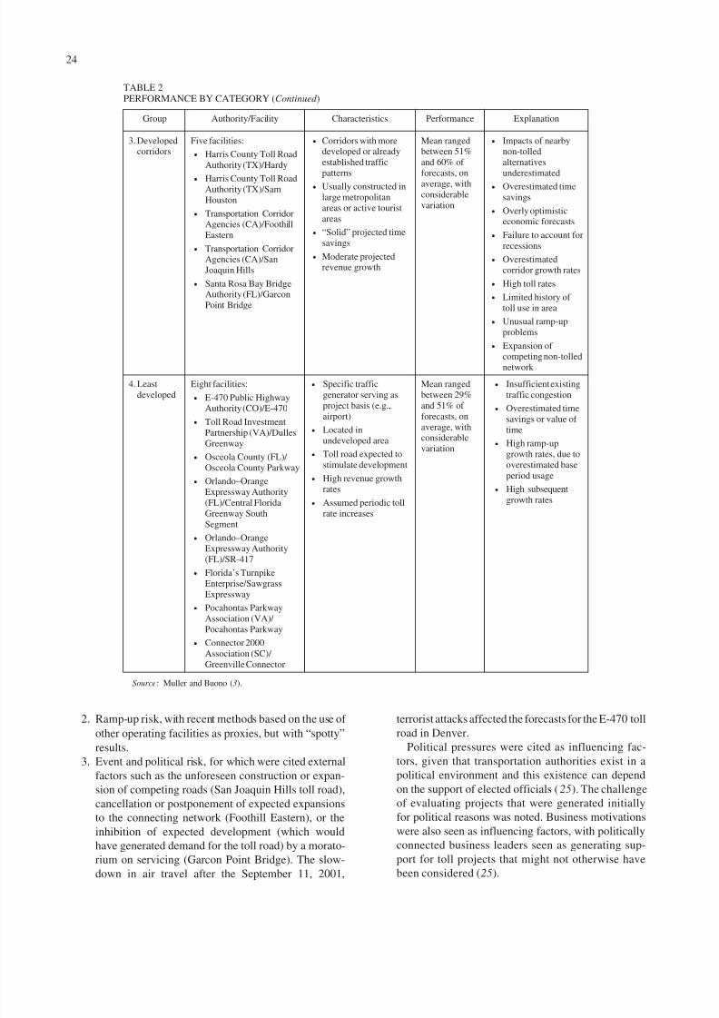
8/3/2019 Estimating Toll Road Demand & Revenue--TRB, 2006
http://slidepdf.com/reader/full/estimating-toll-road-demand-revenue-trb-2006 31/113
2. Ramp-up risk, with recent methods based on the use of
other operating facilities as proxies, but with “spotty”
results.
3. Event and political risk, for which were cited external
factors such as the unforeseen construction or expan-
sion of competing roads (San Joaquin Hills toll road),
cancellation or postponement of expected expansions
to the connecting network (Foothill Eastern), or the
inhibition of expected development (which would
have generated demand for the toll road) by a morato-
rium on servicing (Garcon Point Bridge). The slow-
down in air travel after the September 11, 2001,
24
terrorist attacks affected the forecasts for the E-470 toll
road in Denver.
Political pressures were cited as influencing fac-
tors, given that transportation authorities exist in a
political environment and this existence can depend
on the support of elected officials (25). The challenge
of evaluating projects that were generated initially
for political reasons was noted. Business motivations
were also seen as influencing factors, with politically
connected business leaders seen as generating sup-
port for toll projects that might not otherwise have
been considered (25).
Group Authority/Facility Characteristics Performance Explanation
3. Developedcorridors
Five facilities:
• Harris County Toll Road
Authority (TX)/Hardy
• Harris County Toll RoadAuthority (TX)/Sam
Houston
• Transportation CorridorAgencies (CA)/Foothill
Eastern
• Transportation CorridorAgencies (CA)/San
Joaquin Hills
• Santa Rosa Bay BridgeAuthority (FL)/Garcon
Point Bridge
• Corridors with moredeveloped or already
established traffic
patterns
• Usually constructed in
large metropolitan
areas or active tourist
areas
• “Solid” projected time
savings
• Moderate projectedrevenue growth
Mean rangedbetween 51%
and 60% of
forecasts, on
average, with
considerable
variation
• Impacts of nearbynon-tolled
alternatives
underestimated
• Overestimated time
savings
• Overly optimisticeconomic forecasts
• Failure to account for
recessions
• Overestimated
corridor growth rates
• High toll rates
• Limited history of
toll use in area
• Unusual ramp-up
problems
• Expansion of
competing non-tollednetwork
4. Least
developed
Eight facilities:
• E-470 Public HighwayAuthority (CO)/E-470
• Toll Road Investment
Partnership (VA)/Dulles
Greenway
• Osceola County (FL)/
Osceola County Parkway
• Orlando–Orange
Expressway Authority
(FL)/Central Florida
Greenway South
Segment
• Orlando–OrangeExpressway Authority
(FL)/SR-417
• Florida’s Turnpike
Enterprise/Sawgrass
Expressway
• Pocahontas Parkway
Association (VA)/
Pocahontas Parkway
• Connector 2000
Association (SC)/
Greenville Connector
• Specific traffic
generator serving as
project basis (e.g.,
airport)
• Located in
undeveloped area
• Toll road expected to
stimulate development
• High revenue growthrates
• Assumed periodic toll
rate increases
Mean ranged
between 29%
and 51% of
forecasts, on
average, withconsiderable
variation
• Insufficient existing
traffic congestion
• Overestimated time
savings or value of
time
• High ramp-up
growth rates, due to
overestimated base
period usage
• High subsequent
growth rates
Source: Muller and Buono (3).
TABLE 2PERFORMANCE BY CATEGORY (Continued )

8/3/2019 Estimating Toll Road Demand & Revenue--TRB, 2006
http://slidepdf.com/reader/full/estimating-toll-road-demand-revenue-trb-2006 32/113
25
Another exogenous event was the development of
competing routes or the failure to anticipate network
improvements such as feeder roads or highway inter-
changes. In some situations, noncompetition agreements
have been developed that specify that other government
agencies will not build competing facilities within a cer-
tain protected geographic area. However, the agreements
have not always been implemented.
Survey respondents cited several exogenous factors
that influenced the performance of the forecasts. All of
these concerned the actual conditions under which the
facility operated or was implemented. These factors
included the actual operations and system reliability
(e.g., actual congestion levels, operating speeds, and
incidents); impact of the tolling technology on actual
(recorded) traffic volumes (e.g., owing to unreadable
license plates); violation rate; staging of the facility (or
of other facilities); and changes in policy, mandate,
legislation, ownership, etc.
4. Model error, which reflected the inherent variability in
models regardless of how well the model was cali-
brated and validated [i.e., the forecasts can never repli-
cate the (eventual) actual traffic]. Although a model’s
average error might be small, the average “may mask
a problem, which when compounded within the model
and over time, may severely skew results. This is an
issue that is not discussed in an adequate level of detail
in traffic and revenue reports.” The analysis further
noted that the “simultaneous manifestations” of two or
more of these problems contributed further to the poor
model performance, with the forecasts “[amplifying]
the negative variance between projected and actual
traffic levels.”
Finally, the survey of practitioners found that no single
modeling factor influenced the performance of respondents’
forecasts. Respondents cited as factors the model structure;
the process used to expand the modeled time periods to
annual forecasts; the calibration process, coverage, and pre-
cision; “control” over how the model outputs were used, ana-
lyzed, or interpreted; the lack of transparency/opacity in the
modeling and forecasting process; and the validity (i.e.,
appropriateness) of the model for financing purposes.
TREATMENT OF SPECIFIC FACTORS AFFECTING
FORECAST PERFORMANCE
Drawing on the preceding discussion of the performance of
the forecasts and the underlying reasons, this section exam-
ines the treatment of specific factors that were identified as
part of the scope of the synthesis, in the literature, and by
practitioners.
Demographic and Socioeconomic Inputs
There are two relevant issues. The first concerns the use of
long-range demographic and socioeconomic forecasts (so-
called land use inputs to the model) that may reflect an MPO’s
planning policy (i.e., as the source for these inputs) as
opposed to market trends. Recent toll road demand and rev-
enue forecasts have responded to these concerns by modify-
ing these assumptions to account for input scenarios that were
more conservative and that took into account historical trends
and a more realistic assessment of likely future growth (5
).
An example is provided by a recent (2003) traffic and rev-
enue forecast for the Transportation Corridor System (the
Foothill/Eastern Transportation Corridor and the San
Joaquin Hills Transportation Corridor), in which the local
MPO land use forecasts were reviewed and refined in several
ways: an update to the forecasts according to actual devel-
opment that had occurred in the 5–6 years since the MPOs
had prepared them; a review of job and household growth
rates according to a variety of national, state, and regional
third party sources; interviews with developers, realtors, and
other related interests to identify issues that would affect
future development and the regulatory environment in thestudy area; detailed field studies of 50 “focus areas” to iden-
tify current and potential development capacity and con-
straints to development; and the identification of candidate
areas for redevelopment and infill development at higher
(than originally forecasted) rates in the long term. Forecasts
for different categories of employment were revised accord-
ing to recent trends, and forecasts for residential develop-
ment accounted for such variables as recent changes in
prices. Overall, revised short- and long-term land use fore-
casts were developed (50). The impact of the refined land use
forecasts is not yet clear, given the recentness of the study.
Although the actual revenue growth rates for 2003–2004 and
2004–2005 were greater than the projections (8.7% versus4% and 9.7% versus 4%, respectively), a July 2004 increase
in toll rates might have affected the results (51).
The second issue is the lack of consideration of the impact
of short-term economic fluctuations on travel demand. The
impact of optimistic economic projections on traffic projec-
tions was noted in several studies. The national recession of
1990–1991 affected the use of the first two segments of the
Central Florida Greenway, which had opened in 1989 with
first-year projections just slightly below actual, but with
poorer results for the next two years (over the course of the
recession). A “drag” from the recession was considered to
have affected toll roads in Oklahoma City and Tulsa, Okla-
homa, which opened just after the recession. Local economic
impacts, such as the collapse in oil prices and the subsequent
sharp regional economic downturn of 1986, left economic
growth in the Houston area well below projections, with cor-
responding impacts on the Hardy and Sam Houston toll road
revenues. Even when regional economic activity was close to
the original projections, the performance of some tolled facil-
ities still fell short, because economic activity within the
immediate corridor did not meet projections (e.g., the Saw-
grass Expressway in Florida) or the expected build-out of res-
idential areas was slower than expected (e.g., the Seminole
8/3/2019 Estimating Toll Road Demand & Revenue--TRB, 2006
http://slidepdf.com/reader/full/estimating-toll-road-demand-revenue-trb-2006 33/113
Expressway toll road, also in Florida) (6 ). Practitioners have
begun to consider the impact of short-term economic changes.
The aforementioned Transportation Corridor System forecast
took into account a “recession scenario,” which considered a
“double dip” of below average job gains in the immediate
term, followed by job losses for the next two years, then by a
modest recovery and a recessionary dip in the seventh year.These inputs were used as part of a sensitivity test of the
demand and revenue forecasts (50). Another observer com-
mented that “supply-driven” land use forecasts (meaning
forecasts that take into account factors such as growth in the
labor force, demographics, and productivity) provided more
stable results than did “demand-driven” inputs (such as fore-
casts of population and jobs). The pending retirement of the
“baby boom” generation was also seen to have an impact on
the demand for travel. As an example, this observer cited the
1999 Foothill Eastern refinancing study, which preceded the
aforementioned Transportation Corridor System study. This
study accounted for a more stagnant labor pool after 2010,
which in turn generated “far less” growth in the long-termtraffic and revenue forecasts (3).
A related issue concerns the ability to understand the
travel characteristics of the users of a proposed facility.
With reference to improving the performance of transit rid-
ership forecasts, one observer proposed bringing the fore-
casting horizon closer to the present, which “would reduce
the range of developments that can cause projections to go
awry, such as changes in the local economy or evolution of
travel patterns in response to geographic redistributions of
employment and population.” An “extreme variant” would
be to predict ridership under current demographic and travel
conditions, “which would isolate the increased ridershipattributable to improved transit service from that owing to
demographically induced growth in overall travel demand.”
This “opening-day” ridership would be used as the basis for
the evaluation of alternatives, rather than long-range fore-
casts (35). Although the analytical horizon for toll road
demand and revenue forecasts clearly cannot be shortened,
a current-year or very-short-term toll demand forecast based
on a hypothetical immediate opening of the facility would
allow analysts and users to differentiate the demand that
would result from the network improvement and that would
result from assumed demographic or economic growth. Fur-
ther analyses could test the impact of the facility, with and
without tolls, again in the short-term, to isolate the impactsof tolls. In other words, although these short-term forecasts
might have limited use in the development of absolute esti-
mates of revenues, they would be valuable in grounding and
interpreting the long-range forecasts (i.e., to provide a refer-
ence against which to compare that proportion of forecasted
long-term facility traffic that would use the facility whether
or not the toll is in place or independent of assumed growth).
Travel Characteristics
The availability of appropriate data and the quality of these
data were noted in the literature and in the survey as one of
26
the major sources of potential forecasting inaccuracies (25).
These data include such variables as traffic counts, network
characteristics, travel costs, land use, and employment. Inap-
propriate base year data can result in model validation errors,
which in turn affect all subsequent applications and forecasts.
In practice, these data, which are the foundation of the fore-
casts, were found to be subject to substantial numbers of mea-surement and processing errors (25). Similar problems were
found with forecast inputs such as land use: The model may
accurately reflect the assumed or calculated inputs; however,
if the assumptions are erroneous, then the accuracy of the
forecast will suffer (52).
Current data collection practices are well-established.
They include origin–destination surveys, trip diaries, activity-
based surveys, stated preference surveys, traffic counts, travel
time data, and speed surveys. Surveys of existing socioeco-
nomic and transportation system characteristics are required
for calibration. However, one observer noted that what was
once a standard part of transportation planning is not usuallyundertaken to the same degree in contemporary planning
studies (25). The Minnesota DOT model update noted earlier
used two previous studies (one local and one from California)
as sources of information, given the lack of data (26 ).
Another observer noted the need for caution in the use of
“imported” data to address gaps: “without great care and con-
siderable experience, significant errors can be introduced
into the modelling framework through inappropriate impor-
tation of model parameters.” Other factors relating to data
included the role of uncertainties and potential sources of
error introduced by sampling [in surveys]. The appropriate
categorization of travel markets in terms of their individualvalues of time and willingness to pay was also noted, with
income levels and time sensitivity (i.e., trip purpose) being
important determinants. The ability to save time was the
most important determinant of whether or not a private auto-
mobile driver chooses to use a toll road, whereas truck driv-
ers also took into account the impact on vehicle operating
costs (i.e., that a toll road’s “competitive advantage” for
trucks must be measured both in terms of time savings and
the ability to save on fuel costs and reduce vehicle wear and
tear). Similarly, the importance of “who pays” also was noted,
as was the difficulty in modeling this influence. Finally,
assumptions regarding growth in vehicle ownership (also
related to growth in Gross Domestic Product and income)
were noted as influences on traffic demand in general (53).
These findings generally were corroborated by the sur-
vey of practitioners. Respondents cited the values used for
value of time, willingness to pay, and other monetary val-
ues as influences on the performance of the forecasts. Other
influences included assumptions regarding land use fore-
casts or future network configurations, with some respon-
dents distinguishing public and political influences in these
assumptions; availability, appropriateness, or sufficiency
of the data, models, or analytical processes; environmental
or economic development considerations; and economic cli-

8/3/2019 Estimating Toll Road Demand & Revenue--TRB, 2006
http://slidepdf.com/reader/full/estimating-toll-road-demand-revenue-trb-2006 34/113
27
mate. Overall, respondents recommended collecting more or
better data to improve travel demand forecasting results.
Value of Time and Willingness to Pay
The treatment of the ability and willingness of potential users
to pay was cited as a key performance factor both in the lit-
erature and by practitioners. Values of time can be differen-
tiated by purpose, mode, and/or vehicle class. Willingness to
pay is a variation of value of time that accounts for how much
travelers value different attributes of the toll facility, such as
safety and reliability.
The valuation of travel time is based on two underlying
principles (54). The first principle states that time is valuable
because people can associate it directly with results, such as
making money or participating in a leisure activity—that is,
the time spent in travel could be devoted instead to other
activities. The second principle assumes that time can have
an additional cost over and above that associated with the
first principle; for example, travelers might find it undesir-
able to have to walk, wait for transit, travel on a crowded bus,
or drive in congested conditions. As a result, “the value of
saving time may vary, depending on both the purpose of
travel, which affects the possible alternative uses of time, and
the conditions under which it occurs.”
The measurement of the perceived value of a driver’s
travel time yields the value of time. This influences a driver’s
decision to use a toll road. Values of time vary from region
to region, and what is assumed for one forecast may not be
transferable to another forecast. The value of time is a func-
tion of a driver’s purpose (where work trips are more valu-able than discretionary trips), income, and personality.
The value of time is used to convert the monetary toll to
time. This allows the monetary value to be incorporated into
the model’s generalized cost function. As described earlier in
Methods for Modeling Toll Road Demand, this is incorpo-
rated into the calculation of route diversion (within or post-
trip assignment), which in turn may be fed back to other parts
of the modeling process. Two-thirds of the models reported
in the survey of practitioners incorporated value of time, 10%
used willingness to pay, and another 10% used both. One
model incorporated travel time and travel cost in its mode
choice utility equations.
The choice and derivation of the values used for this deter-
mination are the subject of considerable debate in the litera-
ture. The U.S.DOT has developed a guidance document on
the subject. Its purpose was to establish “consistent proce-
dures” for use by the department in its evaluation of travel
time changes that would result from transportation invest-
ments or regulatory actions. The guidance stated clearly that
locally derived data should be used to forecast demand on
individual facilities (54).
The guidance reviewed the factors that are associated with
the value of travel time. For trips made during work or when
the traveler could vary his or her work hours, the guidance
noted that “the wage paid for the productive work that is sac-
rificed to travel” could be used to represent value of time.
The value of time for other (personal) purposes can be rep-
resented by some fraction of the wage rate. Thus, the hourly
income (before-tax wage rates, including fringe benefits)
could be used as a “standard against which their estimatedvalue of time is measured.” As well, higher income has been
associated with higher values of time, meaning that toll roads
that operate in higher-income areas should experience
greater patronage (and support higher toll rates) (3). The
guidance developed tables that expressed the values of time
(and “plausible ranges”) as percentages of hourly incomes,
categorized by local and intercity travel, business (work-
related) or personal trip purposes, and mode (surface modes
taken together and air travel). A separate category was devel-
oped for truck drivers. A 2003 revision retained the method,
but updated the actual hourly incomes (55).
For toll road demand and revenue forecasts, the value of time generally has been assumed as a single value to represent
an average characteristic for a given study area (25). How-
ever, researchers have recognized that the use of an average
value of time masks the heterogeneity among travelers,
notwithstanding the existing categorizations of time values by
purpose. Recent research examined the preferences of users
of the SR-91 toll lanes (California) by analyzing different
revealed and stated preference survey data sets. The research
concluded that values of time and the value of reliability were
high, although the values dropped for very long distances.
However, these values contained considerable heterogeneity:
to this end, the research examined the impacts of the time of
day at which the trip was made, flexibility of arrival time, gen-der, age, household size, occupation, marital status, and edu-
cation. The research highlighted differences in the data; for
example, drivers with higher incomes were more responsive
to the toll, according to the revealed preference data (i.e.,
according to how they actually behaved), but not according to
the stated preference data. Finally, the data were used to
develop a pricing policy model, which took into account the
utilities calculated for the individual factors (as a means of
illustrating the importance of accounting for heterogeneity in
estimating the value of time) (56 ).
Other researchers identified problems in the application or
development of values of time, as compared with the findings
of empirical studies of what travelers were actually willing
to pay. These included (57 ):
• Trip assignment models that simulated route choice (i.e.,
diversion under tolls) using travel time values that had
been derived from empirical studies of mode choice.
• Application of values of time to choices whose attri-
butes were quite different from those that were used to
calculate the value of time (e.g., comfort, convenience,
and status).
• Relationships between values of time and other influenc-
ing variables (notably, income), which were assumed to

8/3/2019 Estimating Toll Road Demand & Revenue--TRB, 2006
http://slidepdf.com/reader/full/estimating-toll-road-demand-revenue-trb-2006 35/113
develop over time in ways that were inconsistent with
other evidence. [Other empirical studies have suggested
that the value of time increases over time, but not pro-
portionately with income levels (57 )].
• Values of time that were calculated from stated prefer-
ence methods, which must be based on very-short-term
(i.e., immediate) preference structures, but whose resul-tant values are applied to models that reflect behavior
that takes some years to evolve.
The researchers found that in cases where an average
value of time represented a skewed distribution of values,
there was a tendency to overestimate the revenue, and under-
estimate the impact of a toll, because for a given mean value
of time (i.e., for the value of time that was used in the demand
and revenue forecast) there was a smaller number of indi-
viduals who were prepared to pay the toll. To address this,
the researchers recommended the establishment of a relevant
set of purpose-specific, time value distributions; determining
a way to address these distributions in forecasting demand;“growing” the values over time; accounting for the time
values of automobile passengers (in addition to those of the
driver); and establishing methods to convert disaggregated
(heterogeneous) values of time into a single trip value that is
appropriate to the specific project under consideration.
The impact of tolls on shifts in driver behavior over time
is beginning to be understood, as a history of toll facilities
develops from which both static conditions and changes over
time can be observed. In addition to addressing the relative
paucity of data on the subject (given the relative newness of
tolled facilities), historical data are important because driver
behavior can change over time: this, in turn, affects the fore-casts that commonly retain base year rates, modeled relation-
ships, and parameter values through all horizon years. This
was demonstrated by recent research on the Lee County,
Florida, variable pricing program, which found that shifts in
traffic volumes varied over time, with the long-run (3–5
years) relative elasticity of demand being lower than that of
the short run (1 year or less). The research also found that sev-
eral demographic, socioeconomic, and travel behavior factors
affected facility use over time. Drivers who were commuting,
were full-time employees, had more persons in their house-
holds, had a postgraduate degree, and were between 25 and
34 years old were found to be more likely to have increased
their use of the facility. Retired drivers and those with lower
incomes were less likely to use the facility (58).
Two of the studies cited previously also commented on the
use of stated preference surveys as the basis of valuating time
(57 and C. Russell, personal communication, Sep. 20, 2005).
Stated preference surveys attempt to measure the value of
time by presenting hypothetical options to respondents to
quantify how toll rates would affect driver behavior. They are
widely used in toll demand and revenue forecasts. Stated pref-
erence surveys for toll demand forecasting are generally in
28
three parts: (1) background information on a recent trip in the
study corridor, (2) a set of stated preference experiments, and
(3) demographic information. The background information
provides revealed preference data about an actual trip, as well
as baseline data to customize the stated preference scenarios.
The variables of interest are determined and ordered into a
series of scenarios that is presented to respondents as part of the experiments: the scenarios are designed so as to allow the
subsequent estimation of the respondents’ relative prefer-
ences for each of the tested variables. Diversion (multinomial
logit) models and values of time in turn are calculated from
these estimates. Travel time, toll cost, and income typically
are included as attributes, with values of time calculated by
trip purpose (work and non-work) and separately for automo-
biles and trucks. Stated preference surveys in areas that do not
have tolled facilities have tended to result in low values of
time, because respondents express their “anti-toll road senti-
ment.” In areas that have existing toll roads and severe peak-
period congestion, respondents have tended to overestimate
their values of time. In either case, the calculated values of time may have to be recalibrated to reflect actual conditions
more reasonably. The availability of electronic toll collection
(as opposed to cash collection) may also influence the value
of time, in that electronic toll collection users may be less
aware of and, therefore, less sensitive to the total toll paid on
a trip (2), at least in the short term. Another practitioner has
noted that the importance of understanding what (average)
values of time derived from stated preference surveys repre-
sent; namely, they are proxies for several attributes (comfort,
safety, convenience, reliability, etc.) and that all the models
derived from these data assume that the respondent has per-
fect knowledge at the time of his or her decision making
(C. Russell, personal communication, Sep. 20, 2005).
The need for accurate ordering of preferences in the sce-
narios has been noted by some researchers, who examined the
applicability of stated preference surveys, and the methods
used to estimate values of time from them, for toll demand
analysis. The research surveyed a nationwide sample of
respondents on their preferences of 13 alternatives that
described the “essential elements of a commute,” including
congested and uncongested travel times, travel cost (usually,
a toll), and an indication of whether or not trucks were
allowed on the road. The researchers then used the resultant
preferences to calibrate different formulations of the diver-
sion model. They found that the ordering of the preference
scenarios was important and that the choice of model formu-
lation gave “very different ratings” for the same data. Finally,
the research found that the willingness to pay estimates were
relatively low and did not vary much among drivers, which
implied “that the average commuter does not appear willing
to pay much to reduce automobile travel time.” The research
noted that the distribution of willingness to pay was fairly lim-
ited, meaning that few travelers (in the sample) were willing
to pay considerably more than the average toll. The research
concluded that “extreme caution should be used in estimating
stated preferences based upon respondents’ ratings” (59).

8/3/2019 Estimating Toll Road Demand & Revenue--TRB, 2006
http://slidepdf.com/reader/full/estimating-toll-road-demand-revenue-trb-2006 36/113
29
Finally, one study noted the “growing body of empirical
evidence that travelers value reliability as an important factor
in their tripmaking decision.” Reliability generally reflects the
day-to-day variability in expected journey times, owing to
nonrecurrent congestion such as incidents, weather, construc-
tion, and so on. Reliability is considered important in variable-
priced HOT applications, where tolls are adjusted accordingto traffic volumes, to maintain a specified level of service.
Therefore, average travel times on HOT lanes may be only
slightly reduced from those on non-toll lanes; however, the
day-to-day fluctuations in travel time variability are reduced
significantly. Reliability can be critical for travelers with fixed
schedules (such as individuals with daycare pick-ups or those
going to the airport), and is not necessarily correlated with the
traveler’s general value of time. However, there remain few
(if any) operational demand models that account for reliabil-
ity in traveler values of time or that measure the value of reli-
ability, because of a general lack of data: this reflects the few
examples of operational toll roads using variable pricing from
which empirical data can be drawn (29).
Tolling “Culture”
An international review of toll road traffic and revenue fore-
casts demonstrated better performance for countries that had
a “history” of toll roads, compared with those for which road
tolling was new. In “countries with a history of tolling, con-
sumers can be observed making choices about route selec-
tion, effectively trading off the advantages against the costs
of using tolled highway facilities. The consumer response
can therefore be more readily understood by forecasters
preparing predictions for new or extended facility use.” Incontrast, in countries where tolling is new, there are no
revealed preference data on consumer behavior, which
“leaves forecasters more reliant on theoretical survey tech-
niques and assumptions about how drivers may respond to
tolls” (60). The existence of a tolling “culture” also affected
the ramp-up forecasts, with there apparently being “little
transferability of experience between projects (particularly
those in different countries). Ramp-up tends to be project-
specific” (53).
Other influences on traveler choice included the conve-
niences that toll roads offered or were seen to offer.
Improved safety was cited as an influence that would attractdrivers to a “perceived” safer highway, such as one with
fewer trucks (61). Commuters also valued reliability, and
travelers may be willing to pay for predictability of travel
time, especially for time-sensitive activities. The type of toll
collection was cited as a third influence on drivers’ route
choice (61).
Truck Forecasts
The treatment of truck forecasts was the subject of an analysis
that found that the variability associated with such forecasts
was consistently higher than that for light vehicles. Although
truck traffic typically comprises a relatively small portion of
the traffic mix, they commonly pay two to five times and
sometimes as high as 10 times the respective car tariff and so
their contribution to total revenues can be significant. The
choice by trucking firms to use toll roads was also found to
depend on, among other factors, the size of the firm, with inde-pendent owner–operators (that dominate some trucking sec-
tors) being “very sensitive” to tolls (49).
Ramp-Up
The ramp-up period reflects a toll facility’s traffic perfor-
mance during its early years of operation. This period may
be characterized by unusually high traffic growth. The end of
the ramp-up period is marked by annual growth figures that
have (or appear to have) stabilized and that are closer to traf-
fic patterns that have been observed on other, similar facili-
ties. The ramp-up period reflects the users’ unfamiliarity witha new highway and its benefits (“information lag”), as well
as a community’s reluctance to pay tolls (if there is no prior
tolling culture) or to pay high tolls (if there is a history). The
performance of the facility during ramp-up is particularly
important to the financial community, because the “proba-
bility of default is typically at its highest during the early
project years” (9).
As the initial year forecasts in Table 1 indicated, the ramp-
up performance has been problematic and inconsistent. One
analyst noted that the consideration of ramp-up forecasts had
three dimensions (9):
• Scale of ramp-up (i.e., the magnitude of difference
between actual and forecasted traffic).
• Duration of ramp-up (from opening day to beyond
5 years).
• Extent of catch-up [i.e., having experienced lower-than-
projected usage at the time of the facility’s opening, to
what extent could observed traffic volumes catch up
with later year forecasts? The significance of catch-up
volumes, according to one analyst, was that “projects
with lower-than-forecasted traffic during the first year
operations also tend to have lower-than-forecasted traf-
fic in later years (referring to toll and non-tolled roads,
as well as transit and inter-urban rail) (62)].
In other words, the conditions that define ramp-up were spe-
cific to each project, given that the factors that influenced
ramp-up also varied (e.g., signage and marketing, the tolling
culture, and the availability of competing free routes).
Another analyst noted that until recently ramp-up has
largely been ignored. Subsequent efforts have considered
ramp-up; however, these have tended to be based on the use
of other facilities as proxies. However, as more facilities
have opened, actual operations and influencing factors could

8/3/2019 Estimating Toll Road Demand & Revenue--TRB, 2006
http://slidepdf.com/reader/full/estimating-toll-road-demand-revenue-trb-2006 37/113
be observed. An inverse relationship between time savings
and ramp-up has been observed, such that greater time sav-
ings appeared to correlate to a shorter ramp-up (5). As an
example, another analyst noted that the estimates of time sav-
ings for the Hardy and Sam Houston toll roads in the Hous-
ton, Texas, area were very different, with the Hardy saving
less than 5 min per average trip and the Sam Houston savingmore than 10 min. “At some level, this would indicate that
the basic need for the Sam Houston was probably greater”
(which was demonstrated by the significantly better perfor-
mance of the Sam Houston toll road; see Table 1). Also,
income levels along the Sam Houston corridor generally
were higher than those in the Hardy corridor (meaning that
the value of time would be higher for the former) (6 ).
In the absence of extensive observations, however, one
analyst proposed the use of “revenue-adjustment” factors for
ramp-up forecasts. These varied according to the expected
duration of the ramp-up period, the extent to which the ini-
tial observed volumes would have to catch up (i.e., whetherthe initial volumes were less than projections, and by how
much), and the source of the toll demand and revenue pro-
jections (meaning that those commissioned by banks
appeared to be more accurate than those of others, such as the
sponsor; with the former group “typically referred to as ‘con-
servative’ forecasts” and used as the base case in financial
analyses). The factors were derived from a comparison of the
performance of 32 tolled facilities around the world. The fac-
tors ranged from a 10% reduction to first-year revenues for
facilities with a two-year ramp-up and no catch-up required,
according to a bank-commissioned forecast, to a 55% reduc-
tion to first year revenues for facilities with an eight-year
ramp-up and initial volumes 20% less than projected, accord-ing to forecasts commissioned by others (9). However, it
should be noted that although they mask considerable varia-
tion, the averages of the actual versus projected results listed
in Table 1 improve over time, from 59% in the first year to
70% in the fifth year.
An alternative treatment was to recognize the potential for
an extended ramp-up by accounting, in the forecast, for the
market served by the facility; the duration was assumed to be
extended if the facility was “development dependent” and
could also be shortened if it was in a built-up area. The start-
ing point (base forecast) also could be reduced according to
experience on other nearby facilities. This allowed the
“inability to accurately predict a key factor [to be] balanced
by very conservative assumptions” (5).
Time Choice Modeling
The need for models that more accurately capture the dif-
ferences in travel patterns by time of day, day of week, and
even season was identified by the financial community. The
object is twofold: first, to account more explicitly for the
temporal variation in composition of trip purposes, origins
30
and destinations, and vehicle types, including (in addition to
peak-hour travel) the off-peak, midday, night, and weekend
(5). This would replace the common use of factors to expand
peak-hour models to daily and then annual traffic volumes
for purposes of revenue forecasting. It also would replace
the use of 24-h models, from which estimates of hourly traf-
fic volumes must be derived (typically using factors) as thebasis for forecasting diversion under tolls; some MPO mod-
els, which are used as the basis for toll road demand and rev-
enue forecasts, simulate only daily traffic; see, for example,
“Tyler Loop 49—Level 2 Intermediate Traffic and Toll
Revenue Study” (63). Research on the impacts of variable
pricing in Lee County, Florida, found that shifts in trip start
times changed over time; that is, long-run elasticities of
demand were lower than short-run elasticities (58).
The second object is to add and integrate time-of-day
choice with mode and route choice. The Florida Turnpike
Enterprise provides an example of how time-of-day choice
was integrated with modal and route choice. It has relied onwhat it considered best practice in its toll-forecasting proce-
dures for periodic updates of traffic and revenue forecasts, as
well as for the planning, design, and economic feasibility
assessment of proposed new facilities (33). A basic nested
logit approach was used to describe travel behavior for mode,
route, and time of day, with the following choices (33):
• Mode: automobile, drive alone; automobile, two occu-
pants; automobile three plus occupants; bus; and rail.
• Route: tolled or non-tolled roads.
• Time of day: desired travel time or time-shifted trip.
Sixteen statistically estimated nested modal choice mod-els were developed from survey data. These models incor-
porated four time periods and four trip purposes. The models
also included specific decision tree hierarchies for transit and
occupancy classes. Four specific time periods were modeled:
a.m. peak, p.m. peak, midday, and nighttime.
Risk
The need to address risk and uncertainty more comprehen-
sively was cited by the financial community and by
researchers. At the same time, the survey of practitioners
indicated that only a small number of respondents conducted
a risk assessment, with most of the remainder verifying their
results through judgment or reality checks and others not
doing any verification.
Many assumptions and variables must be interpreted and
relied on to complete a traffic and revenue study. The ability
to ensure exactness and accuracy in all of these is limited for
representations of existing conditions as well as forecasts. A
common treatment has been to address uncertainty through
the simple use of conservative assumptions or ranges. How-
ever, this was not always possible, as indicated by some

8/3/2019 Estimating Toll Road Demand & Revenue--TRB, 2006
http://slidepdf.com/reader/full/estimating-toll-road-demand-revenue-trb-2006 38/113
31
survey respondents, who noted the impact on the accuracy of
forecasts of exogenous factors such as public or political
inputs, land use, and network assumptions. For example,
when uncertainties existed about whether a particular com-
peting road would be constructed, it had been the practice to
conservatively assume the competing road would be com-
pleted if it was expected to have a negative impact on the tollfacility. If it was not expected to affect the toll project, it was
then assumed not to be in place (61).
The literature indicated that sensitivity analyses on key
variables was common practice, such as the area growth rate,
value of travel time, planned toll rates, and other variables
that were region-specific or that had shown a high degree of
variability in the past. The SR-520 Toll Feasibility Study for
the Washington State DOT provides an example. The pur-
pose of the toll feasibility study was to determine the revenue
potential and traffic impacts of tolling a replacement bridge
on SR-520. To quantify uncertainty, two tolling objectives
were modeled to “bookend” the upper and lower bound of the reasonable toll possibilities within the corridor (64).
However, respondents to the survey of practitioners recog-
nized that sensitivity analysis might not be sufficient,
because just over half of the respondents stated the need to
conduct more risk assessment in the forecast process. A risk
analysis process can evaluate thousands of different scenar-
ios to quantify the probability of a “range of potential out-
comes” (65).
In other words, it is important, first, to ensure that risk
assessment is incorporated explicitly into the forecasting
process and, second, to make the distinction between the
assessment of risk and other indirect treatments of uncer-tainty (such as judgment or sensitivity analysis). The first is
related, in part, to the inclusion of an appropriate and com-
plete set of assumptions and inputs, and in part to ensuring
that model makers and users of the model outputs all under-
stand the implications of alternative choices or influences
(whether qualitatively or quantitatively).
The second requires a proper understanding of the roles of
the different treatments of uncertainty. For example, some
financial analysts have commented that sensitivity analysis
does not adequately reveal the range of possible outcomes in
a toll road forecast (65). Instead, a range of possible out-
comes could be explored, based on Monte Carlo simulation
and the probability not only of the variables acting as indi-
vidual occurrences but in combination with each other based
on their respective probability of occurrence (65). Another
treatment is offered through “reference class forecasting,”
which uses the experiences of past projects to help statisti-
cally identify the probability of given inputs occurring at a
particular value (36 ).
Toll road demand and revenue forecasts have given little
or no consideration to the possibility of a series of events
occurring simultaneously (65)—for example, if economic
growth recedes, oil prices spike, and a large development that
was scheduled to be in place at the time of the opening of the
toll road is cancelled. Traditional sensitivity analysis typi-
cally took each of these assumptions and varied them one at
a time; however, these assumptions often varied by arbitrary
amounts. A further problem was that in reality, rarely, if ever,
did these assumptions vary from actual outcomes one at atime (65).
Financial analysts have noted that the simultaneous occur-
rence of several vulnerabilities contributed to toll roads gen-
erating lower-than-expected traffic levels and, accordingly,
toll revenues (5). Although risk analysis has been incorpo-
rated into some analyses, one analyst noted that many project
uncertainties were external to the traffic model environment.
Because these uncertainties may not be fully captured in the
model probability analysis, the model outputs must also be
interpreted within the framework of the risk analysis (60).
The National Federation of Municipal Analysts (NFMA)is comprised mainly of research analysts, who are responsible
for evaluating credit and other risks with respect to municipal
securities. NFMA has worked with nonanalyst professionals
in various sectors to develop recommended best practice
guidelines for certain markets, including the toll road demand
and revenue forecasts. In these guidelines, NFMA has
attempted to account for the likelihood that there are many
possible outcomes if future events do not follow the projected
assumptions that are predicted in the model. Given the large
number of input variables required in the modeling process,
NFMA found that the results of forecasts can be significantly
influenced by changes in these inputs (65). Simplistically, by
applying the appropriate background data inputs to the tollforecast, a model could produce a traffic and revenue forecast
that is most likely to occur, often called a base scenario.
Whereas a single best statistical estimate may be desired by
some, there are limitations to a single expected outcome.
A proposed mitigation strategy is the assignment of a
probability distribution to all inputs, or at least to those inputs
identified as most influential to the process. Each individual
variable, with its own probability distribution, can be fluctu-
ated simultaneously. This capability supports a better
approximation of reality then can be obtained, because in
practice variables do not generally change one at a time but
concurrently with varying rates of change (65).
NFMA’s best practices guidelines developed a disclosure
requirements list with respect to creating a range of possible
outcomes for traffic and revenue studies. The list included
the following:
• Creation of a no-build traffic forecast (including truck
and congestion analysis) for the study area, without the
toll road.
• Creation of a baseline traffic and revenue forecast (as
per standard practice).

8/3/2019 Estimating Toll Road Demand & Revenue--TRB, 2006
http://slidepdf.com/reader/full/estimating-toll-road-demand-revenue-trb-2006 39/113
• Sensitivity analysis while simultaneously varying toll
road inputs simultaneously (the following list is a guide
only, but it should be used as the minimum standard):
– Population growth,
– Employment growth,
– Personal income growth,
– Toll elasticity by consumers, and– Acceleration of planned transportation network.
• Debt service analysis with toll road project sensitivity
analysis.
A risk analysis using the Monte Carlo technique was
applied to several factors that were used to develop traffic
and revenue forecasts for a proposed toll road linking Hong
Kong with nearby industrial areas in southern China. The
risk analysis found that whereas variations in the forecasts of
population had insignificant impacts on the traffic and rev-
enue forecasts, the impacts of variability in the trip genera-
tion were very large, with standard deviations of the forecasts
being of the order of double (or more) than the base forecasts.Variations in the estimated diversion rates to the facility and
in the toll rate also were found to be significant. From these
findings, the authors pointed out that the impacts of variabil-
ity and uncertainty in these factors can influence the traffic
and revenue forecasts, and noted that “if the effects of varied
key assumptions and scenario options are not examined, the
real optimal rate of return could be missed” (66 ).
One risk analysis consultant noted that the determination
of risk should not focus on a single outcome but should
explore a range of possible outcomes (D. Bruce, personal
communication, March 4, 2005). This process first deter-
mines the degree of risk in each input variable by developingprobability distributions for all variables. Risk analysis is
carried out by allowing all the underlying variable estimates
to vary simultaneously, which can be done using simulation
techniques such as the Monte Carlo technique. The risk and
uncertainty in the underlying input variable is then translated
into a probabilistic, risk-adjusted forecast of output variables
such as traffic levels, toll rate, revenue, and debt service cov-
erage. Finally, the variables that drive risk, that is to say the
variables that have the greatest influence on the forecast, are
identified.
Bias
The existence of “optimism bias” in transportation projects
has been noted by some observers. “It is in the planning of
such new efforts [referring to projects in a city ‘for the first
time,’ where ‘none existed before’] that the bias toward opti-
mism and strategic misrepresentation are likely to be largest”
(36 ). Another analysis noted the influence of bias on the per-
formance of forecasts, with “systematic optimism bias” cited
as a “distinguishing feature of toll road forecasts.” The analy-
sis recommended that “base case forecasts should be
adjusted to take account of any suspected optimism bias.”
32
Bias was differentiated from “general error” in modeling,
with the performance of traffic forecasts for tolled and non-
tolled roads generally being “very similar.” The update also
suggested the need to consider distributions in error (67 ). On
the other hand, in a project for which multiple bids are
assessed competitively, the forecasts that are used as the
basis of financing, and which are available to the financialcommunity, are those of the winner: the forecasts for the
unsuccessful bids generally will project lower revenues
(D. Johnston, personal communication, Aug. 17, 2005).
The literature review uncovered no formal methods or
guidance to address optimism bias in toll road demand and
revenue forecasts. However, the British Department for
Transport recently developed a guidance document on pro-
cedures to address optimism bias in transportation planning
(68). Although this document addressed the cost side (for
both roads and public transport), its approach could inform
any future discussion of optimism bias in demand forecast-
ing. The guidance document noted that transportation proj-ects always must be considered “risky,” as a result of long
planning horizons and complex interfaces. It was theorized
that optimism bias resulted from a combination of the struc-
ture of the decision-making process and how the decision
makers were involved in the process. Optimism bias was not
an unknown or imaginary phenomenon; rather, it was a log-
ical product of the participants involved, their interests, the
framework for conditions for funding, and the resulting
incentive structure they encounter.
The causes of optimism bias were grouped into four cat-
egories: technical, psychological, economic, and political.
Technical causes included the long-range nature of the plan-ning horizons and that often the project scope and ambition
level can change during the development or implementation
of the project. Psychological causes were explained by a
bias in the mental make-up of the project promoters and
forecasters who can all have reasons to be overly optimistic
in the approval stage—for example, engineers want to see
things built and local transportation officials are keen to see
projects realized. Economic causes were demonstrated by
the argument that if the project went forward and was imple-
mented, then more work was created for the industry; and if
the participants were involved directly or indirectly, there
could be an affecting influence. Finally, political causes
were seen as influencing the perceived optimism bias in
terms of interests, power, and the prevailing institutional
setting that surrounded decision making on transportation
projects.
Project appraisers were seen to have demonstrated a ten-
dency to be overly optimistic. To address this bias, apprais-
ers should make explicit, empirically based adjustments to
the estimates of a project’s costs, benefits, and duration.
These adjustments should be based on data from similar past
projects and adjusted for the unique characteristics of the
project.

8/3/2019 Estimating Toll Road Demand & Revenue--TRB, 2006
http://slidepdf.com/reader/full/estimating-toll-road-demand-revenue-trb-2006 40/113
33
Optimism bias uplifts were introduced as methods of
combating optimism bias in the decision-making process.
They were established as a function of the level of risk that
the British Department for Transport was willing to accept
regarding cost overruns in transportation projects. The gen-
eral principle was that the lower the level of acceptable risk,
the higher the required uplift. The optimism bias upliftsshould be applied to estimated budgets at the time of the deci-
sion to build.
To minimize optimism bias, preliminary findings indi-
cated that formal and informal rules aimed at changing the
established culture should be applied. The following four
benefits to applying optimism bias uplifts to budgets were
identified:
• Emphasis on establishing realistic budgeting as an ideal
while eliminating the practice of overoptimistic bud-
geting as a routine.
• Introduction of fiscal incentives against cost overruns.• Formalized requirements for high-quality cost and risk
assessment at the business case stage.
• Introduction of an independent appraisal process.
Model Validation
Model validation and model calibration are not the same:
Calibration demonstrates how the model (and its individual
components) replicates observed historical data, whereas
validation proposes to demonstrate how “reasonably” the
model’s functional forms and parameters predict actual
observed behavior. It was noted earlier (Explanation of Per-formance) that the inherent model error in toll road demand
forecasts was not addressed, and often masked, by existing
model validation that demonstrated base year forecasts
“near 100% to actual traffic” (5). A thorough evaluation of
toll road demand and revenue forecasts was found to com-
prise three steps: technical quality and merits of the fore-
casting process, interpretation and professional judgment on
forecast results, and risk analysis and sensitivity analysis on
key input variables (25).
A “major criticism of transportation demand models is the
general lack of concern for, and effort put into, the validation
phase of [model development].” Time, budget, and data con-
straints in “typical” practice contribute to this lack of concern;
however, “the improvement in predictive capabilities of
transportation demand models and in the credibility of these
models with decision makers, rests to a large extent on the
analyst’s ability to validate the procedures used.” Three gen-
eral approaches to model validation are described here (12):
• Reasonableness checks of parameters and coefficients—
for example, checking whether or not a particular value
is within an expected range or has the correct sign. The
objective is threefold: to ensure that the model does not
violate theoretical expectations and, if it does, to iden-
tify the source of the error (the model or the expecta-
tion); to ensure that the model does not exhibit any
“pathological tendencies”; and to ensure that it is inter-
nally consistent (meaning that its outputs do not violate
any assumptions used to generate them).
Reasonableness checks of the model outputs also canhelp the user determine whether the forecasts are reason-
able. For example, the projected market for a proposed
tolled facility should be verified to ensure that it is rea-
sonable. Readily available techniques, such as a select
link assignment, could be used. [This technique isolates
which travelers (as measured by trip origins and destina-
tions) are projected to use a particular facility. The tech-
nique then could be used to determine how this subset
of travelers would behave under changes in network
configuration—for example, with or without tolls, or
with or without the facility in place]. However, one con-
sultant noted that many traffic and revenue studies do not
always include this (simple) verification, or a demon-stration of the time advantages offered by the proposed
facility (C. Russell, personal communication, 2005).
• A rigorous test of a model’s predictive capabilities is
provided by using the model to predict demand for a
time period other than that used for the model cali-
bration; this assumes the availability of (at least) a
second set of observed data. The use of the model to
predict some historical condition can be instructive;
for example, in identifying the need to better account
for unforeseen influences (such as conditions of eco-
nomic stagnation).
• When data for multiple time periods are not available, an
alternate (but more restricted) test involves the randomsplitting of the “one-period” data into two sets. One set
is used for calibrating the model, which is then used to
predict the second set’s demand. This allows the model’s
predictive capability to be validated against an indepen-
dent set of data, although the validation is limited by the
lack of temporal difference between the two sets.
The temporal, budgetary, and data constraints posed to
model validation were cited by another traffic and revenue
consultant as fundamental reasons for inaccuracies in toll
road demand and revenue forecasts. In particular, basic data
were often old, incomplete, or unreliable because of limits to
sample size; in turn, this implied that the models that were
developed from these data were subject to “substantial error”
(D. Johnston, personal communication, Aug. 17, 2005).
Peer Reviews
Peer reviews are processes in which external experts (i.e., in
modeling) can provide technical guidance and advice to the
proponent’s team during the course of the development of the
data, models, and forecasts. Peer reviews have been a part of
the toll demand and revenue forecasting process in the past,

8/3/2019 Estimating Toll Road Demand & Revenue--TRB, 2006
http://slidepdf.com/reader/full/estimating-toll-road-demand-revenue-trb-2006 41/113
but on a very limited basis and at a very small scale (5).
Accordingly, the value of the peer review process has been
somewhat limited to date, because the process must be con-
tinuous to show any improvement or advancement of tech-
niques. To benefit from this process, detailed reports must be
prepared and independent meetings conducted with bond rat-
ing agencies to discuss the extent of the review and theresults achieved (5).
The requirements vary for peer reviews for models in U.S.
transportation planning practice. The approaches of FTA,
FHWA, and TMIP are described here.
• FTA has specific requirements and standard review
procedures for forecasting as part of its New Starts
discretionary grant program. These review procedures
were implemented to enable FTA to evaluate and rate
grant applications on an unchanging, unbiased level.
Projects seeking New Starts funding must first pass a
locally driven, multi-modal corridor planning process,which has three key phases; alternatives analysis, pre-
liminary engineering, and final design. The list of
evaluation criteria includes operating efficiencies
(e.g., operating cost per passenger mile) and cost-
effectiveness (e.g., the incremental cost per hour of
transportation system user benefits) (69).
• FHWA allocates funding on a formula basis; meaning
that states and MPOs do not have to compete on a
project-by-project basis for funding. As a result, the same
degree of standardization is not required of forecasting
procedures as in FTA’s New Starts program. However,
FHWA does provide technical assistance to state DOTsand to MPOs in an attempt to ensure that the travel
demand forecasts used are credible and based on proper
planning practice. Three types of assistance are provided
(B. Spears, personal communication, Aug. 18, 2005):
– A checklist of questions that help FHWA, state DOT,
and MPO staff understand what is required of the
model. FHWA staff is encouraged to ask these ques-
tions during the triennial certification reviews that
are conducted with those MPOs with populations of
more than 200,000.
– The creation of a peer review team, whose responsi-
bility is to review the forecasting process and make
recommendations for improvement. These teamstypically include from four to eight travel modelers
from other agencies, MPOs, state DOTs, academia,
or consulting firms, who meet with local planners for
one or two days of review.
– The revision of travel forecasts used in specific proj-
ect documents, such as transportation plans, confor-
mity determinations, and environmental studies.
If a peer review is convened, then several pieces
of information and documentation must be made
available to the team, including an inventory of the
current state of transportation in the area, key plan-
34
ning assumptions used in developing the forecasts,
and descriptions of the methods used to develop fore-
casts of future travel demand (70).
• In addition to its core methodological research, TMIP
reviewed ways to improve existing modeling processes.
To this end, a peer review panel recommended several
types of improvements to the practice of travel demandmodeling, including the peer review process. The rele-
vant recommendations are summarized here (71):
– Land use should be integrated into multiple stages of
the travel demand model, and the integration of land
development patterns into the models is paramount.
– Understanding and incorporation of freight-based
activities into travel demand modeling, because it can
require specialized surveys, and their effect on traffic.
– Migration to activity-based or tour-based modeling
to be conducted only with ample funding, resources,
and proper documentation; otherwise, it is recom-
mended to improve the existing trip-based models.
– Agency creation of coordinated data collectionstrategies and standardization guidelines for regional
modeling.
– Improvement of data quality by supplementing
existing data sources with specialized add-on sur-
veys. This can help to complete data sets that are
incomplete as a result of low survey participation or
inadequate funding.
– Consistency checks undertaken throughout the mod-
eling process.
– Model should be designed to be flexible enough for
a variety of toll and HOV modeling policies to be
evaluated.
– Micro-simulation modeling can be used for moredetailed modeling of areas that have unusual charac-
teristics or that are highly diverse.
– Consideration of time-of-day variables, despite cur-
rent modeling difficulties.
– Agency pooling of resources and sharing of their
experiences through best practice publications.
– High-quality documentation of the components of
and assumptions in agency and region travel demand
models.
One example of the successful use of a peer review, as part
of an overall process, was provided by a toll authority that
responded to the survey of practitioners. This authority has
used its travel demand model for several studies, including
feasibility, policy, investment-grade forecast, design, review
or audit, and state environment analysis studies. For the
analysis of the toll facility feasibility study, the existing model
was updated and enhanced. The success of the forecasting has
been attributed to the regular refinement of the MPO model
(upon which its model is based) over a 10-year period. The
demand and revenue forecasting process has a built-in critical
peer review process. The toll authority has taken a proactive
approach in updating and enhancing a specific aspect of the
model on an annual basis; revalidating the model annually

8/3/2019 Estimating Toll Road Demand & Revenue--TRB, 2006
http://slidepdf.com/reader/full/estimating-toll-road-demand-revenue-trb-2006 42/113
35
using traffic counts, origin–destination surveys, speed and/or
travel time surveys, and land use inputs and network charac-
teristics. The toll authority noted that it has recently received
a rating upgrade on its revenue forecasts.
There are no formal requirements for peer reviews in toll
road traffic and revenue forecasts, although the bond ratingcommunity has called for more and improved reviews (5).
Financial backers do conduct their own “stress tests” of the
revenue and financial forecasts. In addition, as part of its
project oversight and credit monitoring, The Transportation
Infrastructure and Innovation Act, the federal credit assis-
tance program for major surface transportation projects,
requires a project’s senior debt to have the potential to
achieve an investment-grade bond rating. It also requires the
development of an ongoing oversight and credit monitoring
plan for each project, which includes a risk analysis, and
requires that traffic and revenue forecasts be updated and
monitored (72).
In comparison, the general practice in Europe is to con-
duct three sets of forecasts: the grantors of the concession
(the governments); the facility sponsors (proponents); and
the financial backers (lenders, investors, and/or auditors)
(C. Russell, personal communication, 2005). The govern-
ments’ forecasts are normally considered to be overly opti-
mistic, because they are used to develop long-range policies
and plans. The proponents’ forecasts are usually the most
extensive, although they do not always provide the best
results because they are dominated by the model. The finan-
cial forecasts (audits) are usually smaller efforts that are
intended to review the proponents’ forecasts (although more
substantive efforts may follow if the review identifies funda-
mental problems). The audit relies on sensitivity tests,spreadsheet modeling, and stress testing: at the end of the
process, the auditors also must assume responsibility for the
forecast.
The proponents pay for their forecasts as well as those of
the financial backers. As a result, the proponents try to con-
trol the latter’s audit. Some proponents now bring the audi-
tors into the process early, before the lenders are appointed;
this puts some pressure on the auditors, but also provides an
opportunity for them to suggest improvements early in the
process and—by the proponents who have put forward their
case—allows issues generally to be understood.
Conversely, in some places the use of two or more inde-
pendent forecasts for proponents “has been dropped because
(at double the cost) it confuses the audience,” with the result
that—in a “tight bidding timeframe” much effort is wasted
determining who is right, rather than exploring the key risk
issues and refining one approach (D. Johnston, personal
communication, 2005).

8/3/2019 Estimating Toll Road Demand & Revenue--TRB, 2006
http://slidepdf.com/reader/full/estimating-toll-road-demand-revenue-trb-2006 43/113
This chapter identifies checklists and guidelines that could
be used to improve the state of the practice in toll demand
and revenue forecasting. Whereas the preceding chapter
reviewed practices in specific topics, the checklist and
guidelines could provide a framework within which these
topics can be addressed. Three examples are taken from the
literature. They comprise a checklist, guidelines, and an
index: the checklists and guidelines constitute lists of ques-
tions and issues that should be addressed in a toll road
demand and revenue forecast, whereas the index provides away to organize and understand the factors and parameters
that influence the forecast. All are aimed at helping the facil-
ity owner, proponent, and financial analyst (and their mod-
elers) to better understand the process and identify questions
that should be asked in the development of toll road demand
and revenue forecasts.
CHECKLISTS AND GUIDELINES FOR MODELS
Federal transportation planning legislation requires that each
MPO develop a transportation plan as part of its planning
process (70). A transportation plan requires forecasts of future demand for transportation services that are usually
arrived at by using travel demand models. Of specific inter-
est to the toll demand and revenue forecasting community
should be the documentation and access to the planning
assumptions and forecasting methods used in the travel
demand modeling process. FHWA has compiled a checklist
for travel demand forecasting methods, mainly with the pur-
pose of providing a certification review team with an
overview of travel forecasting methods used by MPOs. Spe-
cific examples of important planning assumptions included
in the checklist are:
• Population change (should be compared with past
trends and with statewide demographic control totals).
• Employment change (should be compared with past
trends and with statewide economic growth control
totals).
• Regional distribution of future population, employ-
ment, and land use.
• Demographic change (including automobile owner-
ship, household income, household size, and multi-
worker households).
• Travel behavior change (including telecommuting, trip
chaining, and Internet shopping).
36
Specific examples of important forecasting methods
included in the checklist are:
• Last model revision (i.e., when were new variables,
new algorithms recalibrated with new data?).
• Model specification (i.e., choice of model, specification
of key model coefficients).
• Calibration data (what data were used; e.g., National
Household Travel Survey or Census Transportation
Planning Package).• Local survey (how was the survey conducted, what type
of control?).
• Model validation (what year and data source was the
model validated against?).
• Size of network.
• Number of zones.
• Non-home-based travel (e.g., freight commercial ser-
vices and tourists).
One analyst identified a list of recommended enhance-
ments, from the perspective of the financial community,
which would make the results more acceptable and more
likely to qualify for investment grade status. The recommen-dations included (5):
• Incorporation of a range of possible outcomes given the
low probability that the base case forecast will exactly
match the likely outcome.
• Further study and greater validation of value of time as
an input in forecasting models.
• Further study and greater validation of the ramp-up
effect on start-up toll road facilities.
• More detailed truck traffic analysis as the higher rev-
enue margin created by trucks is an important compo-
nent of a forecast, especially when trucks are projected
to be a significant fraction of traffic.
• Incorporation of the risk and reward of electronic toll
collection with respect to violations and toll evasion
against faster throughput, ease of use, and revenue
recovery through penalties.
• Enhance the investors understanding of the exposure to
modeling while highlighting risk in the final product (i.e.,
enhancing the validation process by validating more than
one year, full disclosure of model limitations, etc.).
In a review of the performance of 14 toll road projects,
another financial analyst identified the key variables and
CHAPTER FOUR
CHECKLISTS AND GUIDELINES TO IMPROVE PRACTICE
8/3/2019 Estimating Toll Road Demand & Revenue--TRB, 2006
http://slidepdf.com/reader/full/estimating-toll-road-demand-revenue-trb-2006 44/113
37
inputs that he believed have had large repercussions, both
positively and negatively, on toll road demand and revenue
forecasts (6 ).
One key variable was economic activity. Although
national economic trends were relevant, the economic activ-
ity within the region and project corridor had a greaterimpact. An example of this is in Harris County, Texas, where
a sharp downturn in oil prices in 1986 left economic growth
in the region well below the projected levels. Particularly
hard hit was the downtown business district, the primary end
destination for many vehicles that were projected to use the
toll road, which caused the forecasted traffic demand to be
considerably lower than was projected.
An input that was constant in all the successful forecasts
was the use of 30% or less as projected revenue growth
over the first 5 years of operation. This low projection
explicitly captured the high initial demand of the road with
no need for toll increases. In contrast, where a very highrevenue growth rate was assumed at the start of the proj-
ect, it indicated a dependency on the growth of these routes
to meet the forecasted revenue. If these growth rates were
not met, the lost revenues were not easily recaptured in the
following years; indeed, the forecast continued to lag
behind initial projections.
Other inputs and variables that appeared most crucial in
the model forecasting process were time saved, the cost of
travel, and the ability or willingness to pay of potential users.
In summary, the most successful forecasts generally had
accurate or even conservative economic forecasts with mod-
erate anticipated growth levels. These toll roads were built incorridors that were fully developed and where congestion
already existed. Another factor was that the corridor income
levels were above the regional levels and time savings were
in excess of 5 min.
GUIDELINES SPECIFIC TO TOLL ROAD
FEASIBILITY STUDIES
The Texas Turnpike Authority (TTA), a division of the
Texas DOT, provides an example of recommended guide-
lines for conducting traffic and revenue studies in support
of toll feasibility analyses (73). The key goals of the guide-
lines were to outline the traffic and revenue reporting
requirements, improve the consistency of assumptions, and
improve quality assurance. Four levels of analysis were
proposed (74):
• Conceptual—determines the potential for a toll road
project to support bonds. (Expected durations of each
type of study were provided and they are listed here as
an indication of the level of effort and detail. The con-
ceptual level had an estimated duration of 1–4 weeks.)
• Sketch—project-specific estimate of costs, demand,
and revenues (6 weeks duration).
• Intermediate—refines the previous analysis, including
a tolling plan. It is expected that demand projects would
be derived from a travel demand model (4–6 months
duration).
• Investment grade—“extensive and detailed” analysis
“to determine its value in anticipation of proceeding to
the bond market” (12–18 months duration).
The guidelines recommended a forecast period of 40
years beyond the opening date of the project. The following
inputs should be taken into account (73):
• Average daily tolled and non-tolled volume,
• Weekday toll transactions,
• Gross annual revenue,
• Tolled length,
• Number of lanes being tolled,
• Truck percentage,
• Opening year automobile and truck toll rate,
• Toll increase increment,
• Period between toll increase, and
• Equivalent revenue days.
The guidelines noted that a lack of consistency on key
assumptions affected the comparability of options. Accord-
ingly, to help ensure consistency and improve comparability,
the following parameters should be considered (73):
• Phased improvement or system implementation scenar-
ios; that is, each tolling point should change in response
to the addition of new tolled segments.
• The definition of the study area should encompassthose transportation facilities that could influence the
candidate toll project. Route classification and lane
configurations of competing facilities should also be
considered.
• Toll diversion assumptions, including general toll
attraction and composite toll attraction. Composite toll
attraction includes ramp-up, electronic toll collection,
toll rate adjustments, and toll utilization.
• Toll transactions estimates are required for all four of
the study levels described previously.
• Traffic growth constraints should be considered, owing
to the long time frame (40 years) of the forecast. Con-
straints could include highway corridor capacity, com-peting toll facilities, economic development, etc.
• Trip rate equivalence or toll equity, which considers
the average toll rate paid by the user traveling all
possible origin–destination paths on the facility. The
toll rates should fall within an acceptable toll rate
ratio.
The TTA has prepared a series of brochures related to
tolling, including a “Toll Feasibility Analysis Guide,” which
summarized the four levels of analytical studies and their
main characteristics (74).

8/3/2019 Estimating Toll Road Demand & Revenue--TRB, 2006
http://slidepdf.com/reader/full/estimating-toll-road-demand-revenue-trb-2006 45/113
38
Another TTA document noted that the major bond rating
agencies looked for the following topics to be addressed as
part of toll road demand and revenue forecasts (2):
• Land use and demographic assumptions, including pop-
ulation and employment information;
• Highway network and alternative routes that are bothfeeding the project or competing with the project;
• Weekday versus weekend traffic;
• Review of travel demand parameter assumptions;
• Trip-making characteristics;
• Truck percentage and generated revenue, because of the
impact trucks can have on toll revenue;
• Peak-period versus off-peak management, especially in
managed lane or congestion pricing projects;
• Value of time;
• Ramp-up period;
• Violation rate;
• Toll rates and increases;
• Point estimate forecasts; and• Economic and political risk.
TRAFFIC RISK INDEX
One financial analyst developed a Traffic Risk Index to
assess and compare the risk associated with a given traffic
and revenue forecast according to 10 facility attributes.
Most of the attributes are divided into subattributes. A
notional scale of from 0 to 10 assessed the risk for each
attribute, with higher values reflecting increasing inherent
uncertainty. Descriptions are provided for each extreme to
help illustrate the range of risk that would be consideredfor the particular subattribute. For example, the fourth
attribute, “forecast horizon,” refers to near-term forecasts
as having the least degree of uncertainty and long-term
(“30+ year”) forecasts as having the greatest uncertainty.
The Index was described as a “starting point for consider-
ing toll-project traffic uncertainty in a logical and consis-
tent manner. The Index also represents a checklist that can
be used to examine project-specific uncertainties andprompt appropriate enquiries (allowing the analyst to draw
his or her own conclusions about the likely reliability of
the resultant forecasts)” (9). The means of assessing the
risk are determined by the user, who also can tabulate or
weight the results at his or her discretion. The Index is
reproduced in Table 3.
SUMMARY OBSERVATIONS
Four observations are useful in summarizing the checklists,
guidelines, and indexes.
• Each attempts to introduce consistency and a system-
atic approach to developing traffic and revenue fore-
casts.
• However, neither method nor the application of the
lists, guidelines, or indexes is specified or prescribed;
rather, these are left to the discretion of the user.
• A large range of attributes is described.
• The types of attributes that are considered varies
according to the perspective: The user (i.e., financial)
community’s lists and indexes generally describe the
conditions and environment within which the traffic
model and forecasts are developed, as well as on the
assumptions and inputs, whereas the modeling commu-nity focuses on the model specification methods.

8/3/2019 Estimating Toll Road Demand & Revenue--TRB, 2006
http://slidepdf.com/reader/full/estimating-toll-road-demand-revenue-trb-2006 46/113
39
ProjectAttribute
0 1 2 3 4 5 6 7 8 9 10
Tolling
regime
• Shadow tolls • User-paid tolls
Tolling
culture
• Toll roads well established-—data on
actual use are available
• No toll roads in the country,
uncertainty over toll acceptance
Tariff
escalation
• Flexible rate setting/escalationformula; no government approval
• All tariff hikes require regulatoryapproval
Forecast
horizon
• Near-term forecasts requirement • Long-term (30+ year) forecasts
Toll facility
details
• Facility already open • Facility at the very earliest stages of planning
• Estuarial crossings • Dense, urban networks
• Radial corridors into urban areas • Ring roads/beltways around urbanareas
• Extension of existing road • Greenfield site
• Alignment: strong rationale (including.tolling points and intersections)
• Confused/unclear road objectives (notwhere people want to go)
• Alignment: strong economics • Alignment: strong politics
• Clear understanding of future highway
network
• Many options for network extensions
exist
• Stand-alone (single) facility • Reliance on other, proposed highwayimprovements
• Highly congested corridor • Limited/no congestion
• Few competing roads • Many alternative routes
• Clear competitive advantage • Weak competitive advantage
• Only highway competition • Multi-modal competition
• Good, high-capacity connectors • Hurry up and wait
Surveys/
data
collection
• “Active” competition protection (e.g.,traffic calming, truck bans)
• Autonomous authorities can do whatthey want
• Easy to collect (laws exist) • Difficult/dangerous to collect
• Experienced surveyors • No culture of data collection
• Up to date • Historical information
• Locally calibrated parameters • Parameters imported from elsewhere(another country?)
• Existing zone framework (widelyused)
• Develop zone framework from scratch
Users:
private
• Clear market segment(s) • Unclear market segments
• Few key origins and destinations • Multiple origins and destinations
• Dominated by single-journey purpose(e.g., commute, airport)
• Multiple-journey purposes
• High-income, time-sensitive market • Average/low-income market
• Tolls in line with existing facilities • Tolls higher than the nor m extendedramp-up?
• Simple toll structure • Complex toll structure (local
discounts, frequent users, variablepricing, etc.)
• Flat demand profile (time-of-day, day-of-week, etc.)
• Highly seasonal and/or peak demandprofile
Users:
commercial
• Fleet operator pays toll • Owner–driver pays toll
• Clear time and operating cost savings • Unclear competitive advantage
• Simple route choice decision making • Complicated route choice decision
making
• Strong compliance with weight
restrictions
• Overloading of trucks is commonplace
Micro-
economics
• Strong, stable, diversified local
economy
• Weak/transitioning local/national
economy
• Strict land use planning regime • Weak planning controls/enforcement
• Stable, predictable population growth • Population forecast dependent on
many exogenous factors
Traffic
growth
• Driven by/correlated with existing,
established, and predictable factors
• Reliance on future factors, new
developments, structural changes, etc.
• High car ownership • Low/growing car ownership
Source: Bain and Wilkins (9).
TABLE 3TRAFFIC RISK INDEX

8/3/2019 Estimating Toll Road Demand & Revenue--TRB, 2006
http://slidepdf.com/reader/full/estimating-toll-road-demand-revenue-trb-2006 47/113
This chapter presents several conclusions and observations
derived from the study. The chapter closes with suggestions
for further methodological and procedural research on toll
road demand and revenue forecasting taken from the litera-
ture and the survey of practitioners.
The survey of practice and the literature corroborated and
detailed several issues of concern, most of which had been
identified in the scope for this synthesis. Several conclusions
were reached.
• Many of the problems that had been identified with the
performance of traffic and revenue forecasts were
related to the applications of the models, less so to
methods and algorithms. In particular, assumptions
regarding land use, network inputs, values of time, and
other inputs; the process of reviewing models and their
results; and the treatment of uncertainties and risks
were most often cited in the literature in explaining why
the performance problems occurred.
It is noteworthy that much of the literature that
describes these problems in the context of toll road
demand and revenue forecasts comes from the financialcommunity, rather than the transportation modeling
community. This suggests a disconnect between the two
communities; the latter being the “traditional” users (and
developers) of the models and the former representing
the new users. The financial community’s concerns also
parallel those of other new users, such as those involved
in air quality conformity analysis, which suggest that the
state of the practice in travel demand modeling has not
kept pace with the issues that the models now must
address. The disconnect is exemplified in different ways;
for example, in the use of risk analysis (incorporating a
range of outcomes) and stress tests (which assess
extreme and multiple “shocks”); neither of which has
been widely applied to transportation planning. Another
example is the treatment of the impact of short-term eco-
nomic recessions on long-range demand forecasts, which
is starting to be considered. A third example is the more
explicit understanding of the role of different economic
influences, such as gender, age, and occupation, on toll
road choice.
It is also incumbent upon the new users to under-
stand how the models work and how to interpret their
results, as well as their inherent limitations; and it is
equally incumbent on the developers of the models and
40
their data to provide this understanding. One traffic
and revenue study reviewed for this synthesis noted
that “professional practices and procedures were used
in the development of the traffic and revenue forecasts
included in this report” as a preface to its overview of
the modeling process, which was brief and did not pro-
vide many details. Doubtless this is true; however, the
ensuing documentation provided very little informa-
tion that could help analysts understand the input or
modeling assumptions, let alone address the questionsposed in the preceding chapter’s checklists. On the
other hand, some traffic and revenue studies provided
considerably more explanation of the modeling proce-
dures and, especially, of the input assumptions and
how they were derived.
• Nonetheless, improvements in both aspects (application
and method) are required to address the performance of
the models in traffic and revenue forecasts.
• Although the application of state-of-the-art method-
ological improvements into common practice—such as
activity-based models and network micro-simulation—
should be expected to improve the state of the practice,
it is likely that these alone will not improve the perfor-mance of traffic and revenue forecasts.
Notwithstanding, several methodological improve-
ments might be made. Two important improvements to
the travel demand modeling process are time-of-day
choice modeling and the modeling of commercial and
truck traffic. The understanding of traveler behavior
when faced with tolls continues to evolve and must be
better understood; that is, a more comprehensive under-
standing of the actual determinants of choice are re-
quired, including values of time and willingness to pay
when confronted with different factors (such as the toll
collection method). The explicit incorporation of risk
and uncertainty in all aspects of the modeling process
also is needed, as is consideration of inputs and outputs
in terms of ranges rather than as absolutes.
It could be argued that each of these areas requires
further research and development before it can be
implemented properly (e.g., the literature indicates that
time-of-day choice modeling is an emerging topic).
Conversely, it also could be argued that simplified (or
better) methods already exist for accounting for each
topic and would represent an immediate improvement
to the forecast if considered (assuming, of course, that
assumptions and methods are treated transparently).
CHAPTER FIVE
CONCLUSIONS

8/3/2019 Estimating Toll Road Demand & Revenue--TRB, 2006
http://slidepdf.com/reader/full/estimating-toll-road-demand-revenue-trb-2006 48/113
41
Finally, more generally, a basic prerequisite to any toll
demand and revenue forecast (and to the ability to
account for any of the previously cited improvements)
must be the ability to model the four components of
travel (generation, distribution, mode choice, and route
choice) as a starting point.
• According to the literature, questions regarding the per-formance of the models and forecasts have been posed
mainly by the financial community, rather than by the
transportation modeling community (with some notable
exceptions). The latter community has focused on
improving the methodological basis of modeling and its
underlying data, as demonstrated by the extensive litera-
ture and research on the topic. However, as suggested in
the previous point, this emphasis has not generally recti-
fied the performance problems. In other words, this
suggests that there is a disconnect between the develop-
ers of the models and their users, with the latter having
evolved from the traditional decision makers to those
with different or more rigorous decision-making criteria.• In turn, this suggests that those in the transportation
community who are making investment decisions
regarding tolled facilities do not always know which
questions to ask of their modeling and forecasting
efforts—in other words, the analytical and modeling
capabilities available to them have not always kept
pace with the needs. This was demonstrated by the
large number of explanations that were cited in the
literature and in the survey as causes of performance
failures. In some cases, the explanations were contra-
dictory; in particular, the financial community cited
application as a key problem, whereas survey respon-
dents cited model method as the problem. This can beexplained in part by the relative newness of toll roads
in some parts of the country and the corresponding lack
of a long-term performance history. It also can be
explained by the changing nature of the tolled facili-
ties, in which parts of a facility (i.e., individual lanes)
are now being tolled: this changes the analytical
requirements significantly. The problem is exacerbated
by the “confidential” or “proprietary” nature of the
forecasts and methods that are developed for toll roads,
and also by “optimism bias” on the part of the sponsor,
local elected officials, or other advocates of the pro-
posed toll road.
• Observers have remarked, informally, that there is no
standardization in the toll road demand and revenue
modeling and forecasting processes. Also, they have
questioned whether such standardization could be pro-
moted in the community. Given that this mirrors a sim-
ilar lack of standardization in travel demand modeling in
general, as noted, that the state of the art in modeling
continues to evolve, and that there are several different
and valid techniques (e.g., as in toll diversion modeling),
it may be more appropriate instead to do two things.
First, standardize the terminology or at least list and cat-
egorize the different definitions for key terms; and sec-
ond, develop a commonly used set of questions and
attributes that should be considered. As an example of
the first, there is no single, commonly understood defini-
tion of what is meant by an “investment grade” traffic
and revenue forecast: it may be more appropriate instead
to develop a list of how different organizations under-
stand, interpret and use this term. An example of the
second is the Texas Turnpike Authority’s guidance (see
chapter four), which provides a practical treatment that
perhaps could be reviewed for general application
across the United States, taking into account the differ-
ent perspectives of the owners, sponsors, and financial
community. The Traffic Risk Index similarly provides
a useful starting point for elaborating on the specific
questions that should be asked (more precisely, the vari-
ables that should be taken into account and their
impacts) in the development of toll road demand and
revenue forecasts.
In their own right, standardizing and understanding
the terminology will not improve the process and
results of traffic and revenue forecasts. However, these
improvements will encourage practitioners and owners
to understand more clearly the objectives and require-
ments of decision makers and financial sponsors, and
ensure in turn that the components of the forecasting
process are more responsive to these needs.
• Several observers have noted that “you get what you
pay for.” In other words, in the United States, sufficient
resources have not been devoted to procuring the
required data or to updating older data, or to calibrating
models to the level of detail that is required. The gen-
eral practice in Europe, for example, is to prepare three
sets of forecasts. This clearly requires an investment on
someone’s part. Intuitively, better data, more detailed
models, and multiple forecasts should improve model
performance. Similarly, it is intuitive that a stronger
role for peer review should improve the performance;
however, the literature review did not uncover any eval-
uations or specific assessments of the effectiveness of
the peer review process for modeling in general.
• It should also be noted that the comparisons in the liter-
ature focused primarily on the revenues as opposed to the
demand (i.e., the traffic and its composition). The litera-
ture noted that revenue performance could be affected by
changes in toll rates or by drawing on reserves, or other
means; in other words, by actions that are not related
directly to demand. Therefore, at least some of the avail-
able information does not accurately reflect the outputs
of the travel demand model and, accordingly, the linkage
between the demand forecasts and the revenue perfor-
mance is not always completely direct or explicit.
Accordingly, there is a need to measure the performance
of the travel demand models in their own right, specifi-
cally examining how well the toll road demand models
simulate each class of vehicle and traveler.
The research literature cited in this synthesis largely
focused on methodological issues; notably, the understanding

8/3/2019 Estimating Toll Road Demand & Revenue--TRB, 2006
http://slidepdf.com/reader/full/estimating-toll-road-demand-revenue-trb-2006 49/113
of the variables that affect the traveler’s decision to use a toll
road, consideration of probability distributions to describe
these variables as a means of analyzing and managing risk,
development of time-of-day choice models, simulation of
value of time and the role of stated preference surveys in esti-
mating value of time or on the development of value-of-time
models based on historical data that are now becoming avail-able. The need for continued research in these areas was
inherent in the literature, with specific recommendations for
research comprising the following.
The financial community and practitioners made several
explicit recommendations for further research.
• Improve understanding of the impact of electronic toll
collection (more generally, the type of tolling collec-
tion) on value of time.
• Incorporate risk analysis into the demand forecasting
process, accounting for multiple possible inputs and
outputs.• Account for the impacts of changed economic condi-
tions (notably, recessions and lower than expected
initial demographic and economic growth).
• Improve the understanding of and the methods for esti-
mating value of time and ramp-up, including the impact
of existing congestion and expected development on
travel demand and on toll road demand specifically.
• Improve the treatment of trucks and commercial vehi-
cles in toll road modeling.
• Improve the validation of the travel demand models.
• Develop a more improved understanding of the factors
and assumptions that are used to develop the demand
models and of the criteria that are used to assess theirperformance and calibration.
A 2005 review of the practice of modeling road pricing by
Spears made the following five recommendations for research.
1. Document case studies of transportation planning
agencies that have incorporated road pricing in their
42
travel models to provide details “concerning changes
in model structure, data requirements, value-of-time
parameters, calibration and validation considerations,
and specific application results from other modeling
efforts.”
2. Compile and synthesize current and past empirical
research on value of time and value of reliability, thencompile the existing research on value of time into “an
application-oriented document that provides travel
modelers with reasonable ranges for [value of time],
classified by income level, trip purpose, or other rele-
vant parameters,” and includes practical guidance on
value-of-time adjustments (such as the impact of elec-
tronic toll collection). A similar compilation of the
more limited research on value of reliability was also
recommended, as well as the identification of priority
areas for additional research and data.
3. Encourage data collection on travel behavior on road
pricing projects. Funding for such projects should
account for additional empirical data collection(notably, on value of time and value of reliability), as
well as for an independent evaluation of the project.
4. Conduct basic and applied research to incorporate
time-of-day and peak spreading models in current
travel demand models to address the “principal limita-
tion” in current travel demand models; that is, “the
way in which they distribute daily trips by time-of-
day.” New methods or models are needed to allow for
more precise resolution of daily trip distributions (by
the hour or half-hour), perform efficient multiclass
assignments over multiple time periods, and allow for
a systematic shift of trips between adjacent time peri-
ods to reflect peak spreading.
5. Conduct basic research to better understand and measure
the influence of traffic congestion (and the underlying
factors that influence congestion on a day-to-day basis)
on travel time variability. Archived operational traffic
data exist to explore this relationship, although they
have been largely unused for this subject.

8/3/2019 Estimating Toll Road Demand & Revenue--TRB, 2006
http://slidepdf.com/reader/full/estimating-toll-road-demand-revenue-trb-2006 50/113
43
1. Regan, E., “Moving Off the Gas Tax Implications for the
Toll Industry,” Tollways, Vol. 1, No. 1, 2004, pp. 2–5.
2. Gustavo, B.A., “Investment-Quality Surveys,” TexasTurnpike Authority, Austin, 2004.
3. Muller, R. and K. Buono, “Start-up Toll Roads: Separat-
ing Winners from Losers,” Municipal Credit Monitor , J.P.
Morgan Securities Inc., New York, N.Y., May 10, 2002.
4. “Private Sector Sponsorship of and Investment in Major
Projects Has Been Limited,” GAO-04-419, General
Accounting Office, Washington, D.C., 2004, pp. 38–52.
5. George, C., W. Streeter, and S. Trommer, “Bliss, Heart-
burn, and Toll Road Forecasts,” Public Finance, Fitch
Ratings, New York, N.Y., 2003.
6. Muller, R., “Examining Toll Road Feasibility Studies,”
Municipal Credit Monitor , J.P. Morgan Securities Inc.,
New York, N.Y., 1996, pp. 1–12.7. “Congestion Pricing—Reducing Traffic Jams Through
Economics,” 1996 [Online]. Available: http://ntl.bts.
gov/DOCS/Fall96_Congestion/Fall96_Congestion.htm.
8. Parsons Brinckerhoff, Texas Transportation Institute,
and Federal Highway Administration, “A Guide for
HOT Lane Development,” Federal Highway Adminis-
tration, Washington, D.C., 2000.
9. Bain, R. and M. Wilkins, “Credit Implications of Traffic
Risk in Start-up Toll Facilities,” Standard & Poor’s,
New York, N.Y., Aug. 15, 2002.
10. English, M., “Environment Risk and Justice,” In Risk
Analysis and Society, T. McDaniels and M.J. Small, Eds.,
Cambridge University Press, United Kingdom, 2004, pp.119–159.
11. Yelds, A. and M. Burris, “Variable Toll Pricing Program
Lee Country, Florida—Revealed Preference Telephone
Survey Findings,” Transportation Research Record
1732, Transportation Research Board, National Research
Council, Washington, D.C., 2000, pp. 42–49.
12. Meyer, M. and E. Miller, Urban Transportation Planning:
A Decision-Oriented Approach, 2nd ed., McGraw–Hill,
New York, N.Y., 2001.
13. Garrett, M. and M. Wachs, Transportation Planning on
Trial: The Clean Air Act and Travel Forecasting, Sage
Publications Inc., Thousand Oaks, Calif., 1996.
14. Delcan Corporation, ADEC Consultants, and iTRANS
Consulting, Costs of Congestion in Canada’s Trans-
portation Sector, Final Report, Transport Canada,
Ottawa, ON, Canada, 2005, pp. 35–39.
15. Boyce, D.E. and Y.-F. Zhang, “Calibrating Combined
Model of Trip Distribution, Modal Split, and Traffic
Assignment,” Transportation Research Record 1607 ,
Transportation Research Board, National Research
Council, Washington, D.C., 1997, pp. 1–5.
16. Levinson, D. and A. Kumar, “Integrating Feedback
into Transportation Planning Model: Structure and
Application,” Transportation Research Record 1413,
Transportation Research Board, National Research
Council, Washington, D.C., 1993, pp. 70–77.
17. Miller, E.J., D.S. Kriger, and J.D. Hunt, TCRP Report 48: Integrated Urban Models for Simulation of Transit
and Land Use Policies: Guidelines for Implementation
and Use, Transportation Research Board, National
Research Council, Washington, D.C., 1998, 251 pp.
18. Chung, J.-H. and K.G. Goulias, “Travel Demand Fore-
casting Using Microsimulation—Initial Results from
Case Study in Pennsylvania,” Transportation
Research Record 1607 , Transportation Research
Board, National Research Council, Washington, D.C.,
1997, pp. 24–30.
19. Shiftan, Y., B.-A., Moshe, K. Proussaloglou, G. de Jong,
Y. Popuri, and S. Bekhor, “Activity-Based Modeling as
a Tool for Better Understanding Travel Behaviour,”Presented at the 10th International Conference on
Travel Behaviour Research, Lucerne, Switzerland,
Aug. 10, 2003.
20. Urban Analytics Inc. and URS Corporation, “Estimating
Demand for Value Pricing Projects—State of the Prac-
tice, Final Draft,” Prepared for North Central Texas
Council of Governments, Arlington, Mar. 26, 2004.
21. Allen, W.G., Jr., and G.W. Schultz, “Congestion-Based
Peak Spreading Model,” Transportation Research
Record 1556 , Transportation Research Board, National
Research Council, Washington, D.C., 1996, pp. 8–15.
22. Van der Zijpp, N.J. and C.D.R. Lindveld, “Estimation of
Origin–Destination Demand for Dynamic Assignmentwith Simultaneous Route and Departure Time Choice,”
Transportation Research Record 1771, Transportation
Research Board, National Research Council, Washington,
D.C., 2001, pp. 75–82.
23. Hague Consulting Group, Halcrow Fox, and Imperial
College London, Modelling Peak Spreading and Trip
Retiming—Phase II , Department for Transport, London,
United Kingdom, 2000.
24. Delcan Corporation, Guiding Framework: Tools for
Urban Energy Use and CO2 Planning, Final Report ,
Natural Resources Canada, Ottawa, ON, Canada, 2001.
25. Dehghani, Y. and W. Olsen, “Potential Pitfalls in Fore-
casting Travel Demand for Toll Roads: Experience in
the US and Overseas,” TRB Paper 99051, 1998.
26. Cambridge Systematics, Inc., and URS Corporation,
MnPass System Study—Technical Memorandum Num-
ber 3, Travel Demand Forecasting Approach, Feb. 3, 2005.
27. Sullivan, E., Continuation Study to Evaluate the Impacts
of the SR 91 Value-Priced Express Lanes—Final Report ,
California Department of Transportation and Cal Poly
University, 2000, 252 pp.
28. Holguin-Veras, J., K. Ozbay, and A. Cerreno, Evalua-
tion Study of Port Authority of New York and New Jer-
sey’s Time of Day Pricing Initiative—Final Report ,
REFERENCES

8/3/2019 Estimating Toll Road Demand & Revenue--TRB, 2006
http://slidepdf.com/reader/full/estimating-toll-road-demand-revenue-trb-2006 51/113
FHWA/NJ-2005-005, Federal Highway Administration,
Washington, D.C., 2005.
29. Spears, B., “Summary of the Current State of the Prac-
tice in Modeling Road Pricing,” Nov. 14, 2005.
30. Vollmer Associates LLP, “183A Project Traffic and
Revenue Study—Final Report,” Central Texas Regional
Mobility Authority, Austin, Dec. 16, 2004.31. Smith, D., C. Chang-Albitres, W. Stockton, and C. Smith,
Estimating Revenues Using a Toll Viability Screening
Tool, FHWA/TX-05/0-4726-1, Federal Highway Admin-
istration, College Station, Tex., Oct. 2, 2004, pp. 9–21.
32. URS Corporation, “Traffic Engineer’s Annual Report
Enterprise Toll Operations,” Florida Department of
Transportation, Tallahassee, Dec. 31, 2004.
33. Dehghani, Y., T. Adler, M.W. Doherty, and R. Fox,
“Development of a New Toll Mode-Choice Modeling
System for Florida’s Turnpike Enterprise,” Transporta-
tion Research Record 1858, Transportation Research
Board, National Research Council, Washington, D.C.,
2003, pp. 9–17.34. Wachs, M., “Ethics and Advocacy in Forecasting for
Public Policy,” Business & Professional Ethics Journal,
Vol. 9, No. 1 & 2, 1990, pp. 141–157.
35. Pickrell, D., “A Desire Named Streetcar—Fantasy and
Fact in Rail Transit Planning,” Journal of the American
Planning Association, Vol. 58, No. 2, Spring 1992,
pp. 158–176.
36. Flyvbjerg, B., M.K.S. Holm, and S.L. Buhl, “How
(in)Accurate Are Demand Forecasts in Public Works
Projects? The Case of Transportation,” Journal of the
American Planning Association, Vol. 71, No. 2, 2005,
pp. 131–146.
37. Giglio, J.M., Jr., “Why Governments Lie—Why Gov-ernments ALWAYS Lie about the Cost of Public
Work Projects—and Why People Want Them to,” The
American Outlook—Ideas for the Future, Vol. 1, 1998,
pp. 19–26.
38. “Mid-Bay Bridge Actual Revenue Growth,” URS Con-
sultants Inc., San Francisco, Calif., Aug. 8, 1995.
39. URS Consultants Inc., and Coverdale & Colpitts, “Traf-
fic and Earnings Report for the Proposed Choctawhatchee
Bay Bridge,” State of Florida Mid-Bay Bridge Authority
Revenue Bonds, Series 1991B, Apr. 1991.
40. “E-470 2003 Actual Revenue Report,” Public Highway
Authority, Aurora, Colo., 2003 [Online]. Available:
www.e-470.com.
41. Vollmer Associates LLP, Hagler Bailly Services Inc.,
Cambridge Systematics Inc., and Felsbur Holt & Ulle-
vig, “E-470 Toll Revenue Study,” E-470 Public High-
way Authority Senior Revenue Bonds, Apr. 26, 2000.
42. Garcon Point Bridge, 2004 Annual Report , Emergency
Transportation Operations, Florida Department of
Transportation, Tallahassee, 2004.
43. URS Consultants Inc., and Coverdale & Colpitts, “Traf-
fic and Earnings Report for the Proposed Garcon
Point–Redfish Point Toll Bridge,” Santa Rosa Bay
44
Bridge Authority (Florida) Revenue Bonds, Series 1996,
Oct. 17, 1996.
44. “Traffic Statistics,” Pocahontas Parkway, Richmond,
Va., 2005 [Online]. Available: http://www.pocahontas
parkway.com/ts.html.
45. Wilbur Smith Associates, “Route 895 Connector Com-
prehensive Traffic and Revenue Study,” PocahontasParkway Association Route 895 Connector Toll Road
Revenue Bonds, June 24, 1998.
46. 2004 Annual Report , Northwest Parkway Public High-
way Authority, Broomfield, Colo., 2004.
47. Vollmer Associates LLP, PBConsult Inc., Cambridge Sys-
tematics Inc., and Carter & Burgess, “Northwest Parkway
Traffic and Revenue Study,” Northwest Parkway Public
Highway Authority Revenue Bonds, June 14, 2001.
48. Summary: Northwest Parkway Public Highway Author-
ity, Credit Analysis, Standard & Poor’s, New York,
N.Y., 2005.
49. Bain, R. and L. Polakovic, Traffic Forecasting Risk:
Study Update 2005: Through Ramp-up and Beyond ,Standard & Poor’s, New York, N.Y., 2005.
50. Vollmer Associates LLP, Final Traffic and Revenue
Report—Transportation Corridor System—Including
the San Joaquin Hills, Foothill and Eastern Transporta-
tion Corridors, 140, Transportation Corridor Agencies,
Calif., Sep. 24, 2003.
51. “The Toll Roads—2005 Annual Reports,” 2005 [Online].
Available: http://www.thetollroads.com/home/annualre
port_2005.htm.
52. Ely, J.L., P.A. Bianchini, A.H. Goldberg, D.W. Green-
baum, and E.J. Regan, “Improving Toll Feasibility
Studies,” International Bridge, Tunnel, and Turnpike
Association, Washington, D.C., 1988.53. “Traffic Risk in Start-up Toll Facilities,” Standard &
Poor’s, New York, N.Y., 2002.
54. “The Value of Saving Travel Time: Department Guidance
for the Valuation of Travel Time in Economic Analysis,”
U.S. Department of Transportation, Washington, D.C.,
Apr. 4, 1997.
55. “Revised Department Guidance: Valuation of Travel
Time in Economic Analysis,” U.S. Department of
Transportation, Washington, D.C., 2003.
56. Small, K.A., C. Winston, and J. Yan, “Uncovering the
Distribution of Motorist Preferences for Travel Time
and Reliability: Implications for Road Pricing,” Univer-
sity of California Transportation Center, Berkeley, Aug.
2002, 42 pp.
57. Hensher, D. and P. Goodwin, “Using Values of Travel
Time Savings for Toll Roads: Avoiding Some Common
Errors,” Working Paper ITS-WP-03-12, University
College London, United Kingdom, 2003.
58. Burris, M.W., K.K. Konduru, and C.R. Swenson,
“Long-Run Changes in Driver Behavior Due to Variable
Tolls,” Transportation Research Record 1864, Trans-
portation Research Board, National Research Council,
Washington, D.C., 2004, pp. 78–85.

8/3/2019 Estimating Toll Road Demand & Revenue--TRB, 2006
http://slidepdf.com/reader/full/estimating-toll-road-demand-revenue-trb-2006 52/113
45
59. Calfee, J., C. Winston, and R. Stempski, “Econometric
Issues in Estimating Consumer Preferences from Stated
Preference Data: A Case Study of the Value of Automo-
bile Travel Time,” The Review of Economics and Statis-
tics, Vol. 83, No. 4, 2001, pp. 699–707.
60. Bain, R. and J. Plantagie, “Traffic Forecasting Risk:
Study Update 2003,” Reason Public Policy Institute,Standard & Poor’s, New York, N.Y., Nov. 6, 2003.
61. Orsi, M., “Start-up Toll Road Facilities,” Paper pre-
sented at National Federation of Municipal Analysts
1996 National Conference, Baltimore, Md., 1996.
62. Flyvbjerg, B., “Measuring Inaccuracy in Travel Demand
Forecasting: Methodological Considerations Regarding
Ramp Up and Sampling,” Transportation Research,
Part A: Policy and Practice, Vol. 39, No. 6, 2005, pp.
522–530.
63. Wilbur Smith Associates, “Tyler Loop 49—Level 2
Intermediate Traffic and Toll Revenue Study,” Final
Report, Texas Turnpike Authority Division, Texas
Department of Transportation, Austin, Mar. 14, 2005.64. Parsons Brinckerhoff, Resource Systems Group, “SR
520 Toll Feasibility Study,” Seattle, Wash., 2004.
65. Bruce, D., “Comments Related to ‘Recommended Best
Practices in Disclosure for Toll Road Financings’,”
Unpublished memorandum, HLB Decision Economics,
Ottawa, ON, Canada, Mar. 4, 2005.
66. Lam, W. and M.L. Tam, “Risk Analysis of Traffic and
Revenue Forecasts for Road Investment Projects,” Jour-
nal of Infrastructure Systems, Vol. 4, No. 1, 1998, pp.
19–27.
67. Bain, R. and J. Plantagie, “Traffic Forecasting Risk:
Study Update 2004,” Reason Public Policy Institute,
Standard & Poor’s, New York, N.Y., Oct. 19, 2004.
68. Flyvbjerg, B. and COWI, “Procedure for Dealing with
Optimism Bias in Transport Planning—Guidance Doc-ument,” British Department for Transport, London,
United Kingdom, 2004.
69. “Introduction to New Starts, Federal Transit Adminis-
tration,” Federal Transit Administration, Washington,
D.C., Jan. 2005 [Online]. Available: www.fta.dot.gov/
16893_ENG_HTML.htm.
70. “Certification Checklist for Travel Forecasting Meth-
ods,” U.S. Department of Transportation, Washington,
D.C., May 27, 2004.
71. “TMIP Peer Review Program Synthesis Report,” Volpe
National Transportation Systems Center, Federal High-
way Administration, Washington, D.C., 2004.
72. “TIFIA Project Oversight and Credit Monitoring Guid-ance,” Transportation Infrastructure and Finance Act
(TIFIA) Joint Program Office, U.S. Department of
Transportation, Washington, D.C., Aug. 4, 2005.
73. “Guidelines for Conducting TTA Traffic and Revenue
Studies,” Technical Memorandum 2005-2, Texas Turn-
pike Authority, Austin, 2005.
74. “Toll Feasibility Analysis Guide,” Texas Department of
Transportation, Austin, 2004.

8/3/2019 Estimating Toll Road Demand & Revenue--TRB, 2006
http://slidepdf.com/reader/full/estimating-toll-road-demand-revenue-trb-2006 53/113
46
“An ETTM Primer for Transportation and Toll Officials,”
Intelligent Transportation Society of America, Washing-
ton, D.C., 1995.Baez, G., “Investment-Quality Surveys,” Texas Turnpike
Authority, Austin, 2004.
Ben-Akiva, M., D. Bolduc, and M. Bradley, “Estimation of
Travel Choice Models with Randomly Distributed Values
of Time,” Transportation Research Record 1413, Trans-
portation Research Board, National Research Council,
Washington, D.C., 1993, pp. 88–98.
Boeuf, P., “Public–Private Partnerships for Transport Infra-
structure Projects,” Nov. 27, 2003.
“Bond Investors, Banks Look Beyond Orange County’s
Financial Fiasco: Special Report—Foothill/Eastern Toll
Corridor,” PWFinancing, Vol. 87, 1995, pp. 17–22.
Brownstone, D., A. Ghosh, T. Golob, C. Kazimi, and D. VanAmelsford, “Drivers’ Willingness-to-Pay to Reduce Travel
Time: Evidence from the San Diego 1-15 Congestion Pric-
ing Project,” 2002 [Online]. Available: http://orion.
oac.uci.edu/~dbrownst1TRBvaltime.pdf.
Cambridge Systematics Inc., and URS Corporation,
MnPASS System Study—Technical Memorandum Num-
ber 4, Evaluation Results, Round 1, Dec. 2, 2004, “Central
City Transportation—A Strategy for Solving the Trans-
port Issues Facing Brisbane’s Central City,” Property
Council of Australia, Sydney, 2005.
Cochran, T.H., “Bang Your Head Slowly: Lessons From
Public–Private Project Finance Remediations in Emerging
Markets,” Mar. 21, 2005.Conference Proceedings 34: International Perspectives on
Road Pricing, International Symposium on Road Pricing,
Nov. 11–19, 2003, 108 pp.
DeCorla-Souza, P., “Clearing Existing Freeway Bottleneck
with Fast and Intertwined Regular Networks: Costs,
Benefits, and Revenues,” Nov. 15, 2003.
DeCorla-Souza, P. and W. Barker, “Innovative Public–Private
Partnership Models for Road Pricing/BRT Initiatives,”
Journal of Public Transportation, Vol. 8, No. 1, 2005.
“Design Manual for Roads and Bridges,” Vol. 12, U.K.
Department for Transport, London, United Kingdom, 1996.
“Developing a Comprehensive Pricing Evaluation Model for
Managed Lanes,” Various, FY04-RMC2-0-1818, 2005.
Dial, R.B., “Network Optimized Congestion Pricing: A Para-
ble, Model, and Algorithm,” U.S. Department of Trans-
portation, Washington, D.C., May 1, 1995, 36 pp.
Eisenhardt, P., “Making Managed Competitions Fair,”
PWFinancing, Vol. 97, 1996.
Evans, J.E. and K.F. Turnbull, TCRP Report 95: Road Value
Pricing: Traveler Response to Transportation System
Changes, Transportation Research Board, National
Research Council, Washington, D.C., 2003, pp. 14–67.
Fairweather, N.B., “Response to the Government Consulta-
tion on Developing and Integrated Transport Policy,”
Department for Transport, London, United Kingdom, 1999
[Online] Available: http://www.dft.gov.uk/itwp/consult/
index.htm.“Final E-470 Bonds Rated,” PWFinancing, Vol. 139, 2000,
pp. 6–8.
“Financial, Economic, and Social Topics in Transportation,”
Transportation Research Record 1576, Transportation
Research Board, National Research Council, Washington,
D.C., 1997.
Flyvbjerg, B., “Bringing Power to Planning Research: One
Researcher’s Story,” Presented at the London School
of Economics and Political Science Planning Research,
London, United Kingdom, 2000.
Flyvbjerg, B., “Good Practice Lessons from the Urban Traffic
Project, Denmark,” Presented at Conference on Good Prac-
tice in Integration of Environment into Transport Policy,European Commission, Brussels, Belgium, Nov. 10, 2002.
Flyvbjerg, B., M.K.S. Holm, and S.L. Buhl, “Underestimat-
ing Cost in Public Works Projects—Error or Lie?” Amer-
ican Planning Association Journal, Vol. 68, No. 3, 2002,
pp. 279–295.
Flyvbjerg, B., M.K.S. Holm, and S.L. Buhl, “How Common
and How Large Are Cost Overruns in Transport Infra-
structure Projects?” Transport Reviews, Vol. 23, No. 1,
2003, pp. 77–88.
Flyvbjerg, B., M.K.S. Holm, and S.L. Buhl, “Cost Under-
estimation in Public Works Projects: Error or Lie?—
Paper,” 2004.
Flyvbjerg, B., M.K.S. Holm, and S.L. Buhl, “What CausesCost Overrun in Transport Infrastructure Projects?”
Transport Reviews, Vol. 24, No. 1, Jan. 2004, pp. 3–18.
George, C., W. Streeter, and S. Trommer, “Redefining Toll
Roads: An American Challenge,” Public Finance, Fitch
Ratings, New York, N.Y., 2003, pp. 1–16.
George, C., S. Trommer, and M. McDermott, “The Continu-
ing Search for Bliss: Flexible Toll Road Structures,” Public
Finance, Fitch Ratings, New York, N.Y., 2004.
Hague Consulting Group, Halcrow Fox, and Imperial College
London, “Modelling Peak Spreading and Trip Retiming—
Phase II,” Department for Transport, London, United
Kingdom, 2000.
Halloran, J.V., III, “Standardizing Electronic Toll Collec-
tion,” Policy Insight No. 149, Reason Public Policy Insti-
tute, Los Angeles, Calif., 1992, 31 pp.
Henk, G., “Design-Build Procurement Innovations: The
Benefits Exceed the Challenges,” PWFinancing, Vol. 94,
1996, pp. 12–14.
Hensher, D. and P. Goodwin, “Using Values of Travel Time
Savings for Toll Roads: Avoiding Some Common Errors,”
Working Paper ITS-WP-03-12, University College London,
United Kingdom, 2003.
Holguin-Veras, J., K. Ozbay, and A. Cerreno, “Evaluation
Study of Port Authority of New York and New Jersey’s
BIBLIOGRAPHY

8/3/2019 Estimating Toll Road Demand & Revenue--TRB, 2006
http://slidepdf.com/reader/full/estimating-toll-road-demand-revenue-trb-2006 54/113
47
Time of Day Pricing Initiative—Final Report,”
FHWA/NJ-2005-005, Federal Highway Administration,
Washington, D.C., 2005, 492 pp.
“Information Requirements for Transportation Economic
Analysis,” Vol. 21, Transportation Research Board,
National Research Council, Washington, D.C., Aug. 19,
1999.“Innovative Transportation Financing,” American Association
of State Highway and Transportation Officials, Washington,
D.C., 1995, 800 pp.
Jones, J. and F. Nix, “Highway Finance Theory and Prac-
tice,” No. 2, TAC, 1999.
“Land Use and Transportation Planning and Programming
Applications,” Transportation Research Record 1617 ,
Transportation Research Board, National Research Coun-
cil, Washington, D.C., 1998.
Larsen, O. and K. Ostmore, “The Experience of Urban Toll
Cordons in Norway—Lessons for the Future,” Transport
Economics and Policy , Vol. 35, Part 3, 2001, pp. 457–471.
Mackie, P.J., M. Wardman, A.S. Fowkes, G. Whelan, andJ. Nellthorp, “Values of Travel Time Savings in the
UK,” University of Leeds in association with John Bates
Services, Institute for Transport Studies, Leeds, United
Kingdom, 2003.
Mekky, A., “Forecasting Toll Revenues for Fully Electronic
Highways Operating Under Transponder and Video-
Imaging Systems,” Transportation Research Record
1607 , Transportation Research Board, National Research
Council, Washington, D.C., 1999, pp. 11–22.
Mierzejewski, E.A., An Assessment of Uncertainty and Bias:
Recommended Modifications to the Urban Transportation
Planning Process, Ph.D. Dissertation, Department of Civil
and Environmental Engineering, University of SouthFlorida, Tampa, 1996.
Mokhtarian, P., I. Salomon, and S. Choo, “Data and Measure-
ment Issues in Transportation, with Telecommuting as a
Case Study,” UCD-ITS-RR-04-29, University of California
at Davis, 2004.
Muthuswamy, S., D. Levinson, P. Michalopoulos, and
G. Davis, “Improving the Estimation of Travel Demand for
Traffic Simulation: Part I,” CTS 04-11, Civil Engineering
Department, University of Minnesota, Minneapolis/
St. Paul, 2005.
“New Brunswick Toll Highway Project—Traffic and Rev-
enue Forecasts,” Canadian Highways International Cor-
poration, Mississauga, ON, Canada, Nov. 30, 1994.
Parsons Brinckerhoff, “Truck Only Toll Facilities: Potential
for Implementation in the Atlanta Region,” State Road and
Tollway Authority, Atlanta, Ga., Apr. 1, 2005.
Passantino, G., “Study Recommends Removal of Tollbooths,
Increase Use of Tolls,” Reason Public Policy Institute,
Los Angeles, Calif., Nov. 30, 2000.
Pietrzyk, M.C. and E.A. Mierzejewski, NCHRP Synthesis of
Highway Practice 194: Electronic Toll and Traffic Man-
agement ( ETTM ) Systems, Transportation Research
Board, National Research Council, Washington, D.C.,
1993, 63 pp.
Poole, R., Jr., “Introducing Congestion Pricing on a New
Toll Road,” Transportation Research Record 1359, Trans-
portation Research Board, National Research Council,
Washington, D.C., 1992, pp. 19–26.
Poole, R., Jr., “Introducing Congestion Pricing on a New
Toll Road,” Policy Insight No. 150, Reason Public Policy
Institute, Los Angeles, Calif., 1992, 18 pp.Poole, R., Jr., “Privatizing Wisconsin’s Interstate Highway,”
Policy Study No. 203, Reason Public Policy Institute,
Los Angeles, Calif., 1996.
Poole, R., Jr., “California Toll Roads Take Opposite Paths,”
Reason Foundation, Los Angeles, Calif., Nov. 15, 2002.
Poole, R., Jr., “A Win–Win Solution for Our Freeways
(High-Occupancy Toll Lane Systems Ease Traffic While
Raising Revenue),” Reason Foundation, Los Angeles,
Calif., Aug. 29, 2003.
Poole, R., Jr., “Corridors for Toll Truckways: Suggested
Locations for Pilot Projects,” Policy Study No. 316 , Rea-
son Foundation, Los Angeles, Calif., 2005.
Poole, R., Jr., and J.R. Guardiano, “The Market for PrivateToll Projects in the United States,” Policy Insight No.
140, Reason Public Policy Institute, Los Angeles, Calif.,
1992, 71 pp.
Poole, R., Jr., and C.K. Orski, “Building a Case for Hot
Lanes: A New Approach to Reducing Urban Highway
Congestion,” Policy Insight No. 257 , Reason Public Pol-
icy Institute, Los Angeles, Calif., 1995.
Poole, R., Jr., and C.K. Orski, “HOT Networks: A New Plan
for Congestion Relief and Better Transit,” Policy Insight
No. 305, Reason Public Policy Institute, Los Angeles,
Calif., 2003.
Poole, R., Jr., P. Samuel, and B. Chase, “Building for the
Future: Easing California’s Transportation Crisis with Tollsand Public–Private Partnerships,” Policy Study No. 324,
Reason Foundation, Los Angeles, Calif., 2005.
Poole, R., Jr., K. Soucie, D. Fleming, and T. McDaniel,
“Rebuilding the Marquette Interchange Via a Public–
Private Partnership,” Policy Study No. 304, Reason Foun-
dation, Los Angeles, Calif., 2003.
Poole, R., Jr., and Y. Sugimoto, “Congestion Relief Toll
Tunnels,” Policy Study No. 164, Reason Public Policy
Institute, Los Angeles, Calif., 1993, 32 pp.
PriceWaterhouseCoopers, Global PPP/Infrastructure Year-
book 2005, 2005.
“Recommended Best Practices in Disclosure for Toll Road
Financings,” National Federation of Municipal Analysts,
Pittsburgh, Pa., 2005, 25 pp.
“Review of Travel Demand Modeling by the Metropolitan
Washington Council of Governments,” Transportation
Research Board, National Research Council, Washington,
D.C., Sep. 8, 2003.
“Revised Department Guidance: Valuation of Travel Time in
Economic Analysis,” U.S. Department of Transportation,
Washington, D.C., 2003.
Rusch, W.A., NCHRP Report 117: Toll Highway Financing,
Transportation Research Board, National Research Coun-
cil, Washington, D.C., 1984, 29 pp.

8/3/2019 Estimating Toll Road Demand & Revenue--TRB, 2006
http://slidepdf.com/reader/full/estimating-toll-road-demand-revenue-trb-2006 55/113
portation Research Board, National Research Council,
Washington, D.C., 1999.
“Transportation Finance, Pricing, and Economics,” Trans-
portation Research Record 1732 , Transportation Research
Board, National Research Council, Washington, D.C.,
2000.
“Transportation Finance, Training, Strategic Management,and Economic Analysis,” Transportation Research
Record 1498, Transportation Research Board, National
Research Council, Washington, D.C., 1995.
“Transportation Forecasting and Travel Behavior,” Trans-
portation Research Record 1607 , Transportation Research
Board, National Research Council, Washington, D.C., 1997.
Urban Analytics Inc., and URS Corporation, “Estimating
Demand for Value Pricing Projects—State of the Practice,
Final Draft,” Prepared for North Central Texas Council of
Governments, Arlington, Va., Mar. 26, 2004.
URS Consultants Inc., “Mid-Bay Bridge Actual Revenue
Growth,” State of Florida Mid-Bay Bridge Authority Rev-
enue Bonds, Aug. 8, 1995.URS Corporation, Traffic Engineer’s Annual Report Enter-
prise Toll Operations, Florida Department of Transporta-
tion, Tallahassee, Dec. 31, 2004.
Van Ceenhuizen, M. and P. Nijkamp, “Coping with Uncer-
tainty—An Expedition in the Field of New Transport
Technology,” Research Memo 2001-9, Falculteit der
Economische Wetenschappen en Bedrijfskunde, 2001.
Vollmer Associates LLP, “Traffic and Revenue Report and
Review of Operating and Maintenance Expenses—
Delaware River & Bay Authority,” Dec. 2, 2002.
Vollmer Associates LLP and HDR Engineering Inc.,
“System Traffic & Earnings Report,” Jan. 31, 2003.
Wachs, M., “When Planners Lie with Numbers,” AmericanPlanning Association Journal, Vol. 55, No. 4, 1989,
pp. 476–479.
Wilbur Smith Associates, “The Potential for Variable Pricing
of Toll Facilities—Draft Report,” DTFH61-93-C-00055,
Federal Highway Administration, Washington, D.C.,
Aug. 30, 1995.
Wilbur Smith Associates, “Executive Summary Preliminary
Financing Program for Toll Highways in Arkansas,” 2002.
Wilbur Smith Associates, “SR 16 Tacoma Narrows Bridge
Traffic and Revenue Study,” 2002.
Wilbur Smith Associates, IBI Group, and Resource Systems
Group, “Comprehensive Traffic and Revenue Study
Highway 407 Toll Road,” Ontario Transportation Capital
Corporation, Canada, 1996.
Willumsen, L., “European Transport Policy: Ideas for
Emerging Countries,” 2005.
Wu, Y., G. David, and D. Levinson, “Improving the Estima-
tion of Travel Demand for Traffic Simulation: Part II,”
CTS 04-11, Civil Engineering Department, University of
Minnesota, Minneapolis/St. Paul, 2004.
Wuestefeld, N., “Recent Toll Road Innovations,” PWFi-
nancing, Vol. 66, 1993, pp. 24–25.
48
Samuel, P. and R. Poole, Jr., “Should States Sell Their
Toll Roads?” Policy Study No. 334, Reason Foundation,
Los Angeles, Calif., 2005.
Small, K., “I-15 Congestion Pricing Project Monitoring and
Evaluation Services—Worldwide Experience with Con-
gestion Pricing,” San Diego State University Foundation,
Calif., June 10, 1997.Small, K.A., R. Nolan, X. Chu, and D. Lewis, NCHRP
Report 431: Valuation of Travel–Time Savings and Pre-
dictability in Congested Conditions for Highway User-
Cost Estimation, Transportation Research Board, National
Research Council, Washington, D.C., 1999, 80 pp.
Smith, D., C. Chang-Albitres, W. Stockton, and C. Smith,
“Estimating Revenues Using a Toll Viability Screening
Tool,” FHWA/TX-05/0-4726-1, Federal Highway Admin-
istration, College Station, Tex., Nov. 2, 2004, pp. 9–21.
Spear, B., “A Summary of the Current State of the Practice
in Modeling Road Pricing,” Presented at the Expert
Forum on Road Pricing and Travel Demand Modeling,
Alexandria, Va., Nov. 14–15, 2005.Spock, L.M., NCHRP Synthesis of Highway Practice 262:
Tolling Practices for Highway Facilities, Transportation
Research Board, National Research Council, Washington,
D.C., 1998, 54 pp.
Sullivan, E., “Evaluating the Impacts of the SR 91 Vari-
able—Toll Express Lane Facility Final Report,” Applied
Research and Development Facility, California Polytech-
nic State University, San Luis Obispo, 1998.
Texas Transportation Institute and Various, “Toll Viability
Screening Tool Workshop,” Project 0-4726, Aug. 6, 2004.
Tillman, R., “Shadow Tolls,” Civil Engineering, Vol. 68,
No. 4, Apr. 1998, pp. 51–53.
“TMIP Peer Review Program Synthesis Report,” VolpeNational Transportation Systems Center, Federal High-
way Administration, U.S. Department of Transportation,
Washington, D.C., 2004.
“Toll Reports,” 1997 [Online]. Available: http://www.dot.ca.
gov/dist12/doc/programs.htm.
“Tollways—The Learning Issue,” International Bridge,
Tunnel, and Turnpike Association, Vol. 1, No. 2, 2005.
“Tolling Concepts Guide, Advanced Toll Collection Sys-
tems,” Texas Department of Transportation, Austin, 2006.
“Transportation and Public Policy 2002,” Transportation
Research Record 1812, Transportation Research Board,
National Research Council, Washington, D.C., 2002.
“Transportation Finance, Economics, and Management,”
Transportation Research Record 1649, Transportation
Research Board, National Research Council, Washington,
D.C., 1998.
“Transportation Finance, Economics, and Strategic Manage-
ment,” Transportation Research Record 1558, Trans-
portation Research Board, National Research Council,
Washington, D.C., 1996.
“Transportation Finance, Economics, Pricing, and Manage-
ment, Transportation Research Record 1659, Trans-

8/3/2019 Estimating Toll Road Demand & Revenue--TRB, 2006
http://slidepdf.com/reader/full/estimating-toll-road-demand-revenue-trb-2006 56/113
49
All-or-nothing assignment—assignment approach in which
all travel demand for each origin–destination pair is
assigned to the shortest time path based on uncongestedtravel times.
Barrier toll road—has one or more toll plazas that form a bar-
rier across the roadway to prevent free passage. Motorists
are required to pay a toll to continue, and the system usu-
ally includes large mainline toll plazas and small toll
plazas at on and off ramps.
Closed barrier toll—a system that does not allow motorists
to enter the roadway network without first paying a fee.
Generally a payment or a ticket is issued at the entry and
exit points in the roadway network.
Electronic toll and traffic management (ETTM)—the use of
two-way electronic communications between moving
vehicles and roadside sensors for the purposes of toll col-lection and other traffic management functions.
Electronic toll collection (ETC)—the use of automatic elec-
tronic vehicle identification, such as transponders, for non-
stop toll collection.
Equilibrium assignment—a trip assignment algorithm that
takes into account the build-up of volume and the ensu-
ing changes in trip time when allocating trips to links.
From the traveler’s perspective, the assignment simu-
lates the driver’s desire to minimize overall his or her
travel time (i.e., his or her travel costs) between a partic-
ular origin and destination by switching paths. Equilib-
rium occurs when the travel time on all possible paths for
a given origin–destination is equal—that is, the driver no
longer can improve his or her overall trip time by switch-
ing paths. Equilibrium is achieved, usually after several
iterations, when the difference in overall travel time (i.e.,
in generalized cost) summed over all trips and all origin–
destination pairs is very small, between the current and
previous iterations (i.e., is within specified absolute
and/or percentage differences).
Feed-back loops—part of the iterative modeling process
where at the completion of the travel demand assign-
ment, the resulting travel times or costs are fed back into
trip generation, trip distribution, or mode split steps. The
next iteration takes into account these travel costs foreach origin–destination pair and recalculates the travel
demand.
Goodness of fit measures—used to validate models. Com-
monly used measures include the following:
Absolute comparison of the absolute difference between
modeled flow and observed flow, on a given link or across
a screenline.
Relative comparison of difference between the modeled
flow and the observed flow. That is, modeled flow divided
by observed flow, with the comparison typically expressed
as a percent.
GEH statistic combines the absolute and relative com-
parisons. It accounts for two types of error: that associ-
ated with the simulated flow (reflecting the fit of themodel) and that associated with the observed flow
(through data collection errors and the day-to-day vari-
ability of traffic).
The statistic is defined as:
The statistic is defined as:
The GEH is properly a goodness of fit measure, rather
than a statistical test. It is intended to give a quick indi-
cation of how well the model is working. It can, and nor-
mally is, applied to all model links for which observed
counts are available. R2 is the correlation coefficient of the best-fit regression
line of a plot of the modeled flows versus observed
flows. This measure is commonly used to compare flows
across a number of links, whether or not they are part of
the same screenline or route (for example, all arterials in
an urban network for which traffic counts are available).
Correlation coefficients closer to 1.0 indicate a better
goodness of fit.
Open barrier toll—a system that allows motorists to enter the
roadway network at certain locations without immediate
payment prevents the motorist from proceeding past cer-
tain points, unless a fee is paid. It can use electronic toll
collection, which offers drivers the ability to pay tolls
without stopping.
Open road tolling—a system with no physical toll booths. All
tolling is conducted by the identification of vehicles pass-
ing under a gantry at each individual tolling point. Tolls
are collected by one of two methods including electronic
toll collection or video license plate identification system.
Shadow toll—a payment and revenue process where instead
of charging the user directly, businesses, land holders, or
government agencies reimburse the private investor by
accounting for the number and type of vehicles using the
road, therefore allowing the private sector to invest the
capital and the beneficiaries of the toll road to pay per theusage of the facility by the public.
Stress test—used to assess the financial stability of a
project (or of a portfolio of projects). The process reval-
ues the project’s financial performance according to a
different set of assumptions in the face; for example,
of unforeseen “shocks.” Most asset markets lack a his-
tory of returns that provide sufficient information about
the behavior of markets under extreme events: stress
tests complement traditional financial forecasting mod-
els by testing how the project’s value changes in
response to “exceptional but plausible” changes in the
GEHobserved flow simulated flow
obs=
−
×
( )
. (
2
0 5 eerved flow simulated flow− )
GLOSSARY

8/3/2019 Estimating Toll Road Demand & Revenue--TRB, 2006
http://slidepdf.com/reader/full/estimating-toll-road-demand-revenue-trb-2006 57/113
underlying risk factors. In addition to testing “market
risk” [such as toll revenues less than projected], the
process also examines credit risk (losses from borrower
defaults) and liquidity risks (illiquidity of assets and
depositor runs). Several techniques have been developed
in recent years.
50
Violation rate—a measure of the vehicles that are illegally
evading the tolls compared with the number of vehicles
using the tolled facility. Examples of toll evasion include, but
are not limited to, the following: screening of license plates,
using HOT lanes without the proper number of people, or
using improper electronic pass with an unregistered vehicle.

8/3/2019 Estimating Toll Road Demand & Revenue--TRB, 2006
http://slidepdf.com/reader/full/estimating-toll-road-demand-revenue-trb-2006 58/113
51
OVERVIEW OF METHOD
A survey was conducted regarding the practice of toll facil-
ity demand revenue estimates. This survey of practitioners
was sent to four specific agency types: state departments of
transportation (DOTs), toll authorities, bond rating agencies,
and bond insurance agencies. The first two types represent
the traditional developers and users of traffic forecasts. The
inclusion of the financial community (the latter two types)
was intended to capture the viewpoints and experiences of
the forecasting and modeling process from as many partici-
pants involved in the process as possible.
Participants were given the option of answering directlyonline through a web-based survey program (Websurveyor),
or completing a hardcopy of the survey, which was included
in the e-mail as a pdf (in which the survey form could be
returned to the consultant by mail or fax).
SURVEY OF PRACTICE
Survey Development
The survey was conducted over a two-month period in April
and May 2005. Before the survey was distributed, it was nec-
essary to establish a comprehensive outline and to test the
survey to ensure that it was as accurate and target-specific aspossible.
During the initial stages of the survey design, it was deter-
mined that the survey should be completed by several differ-
ent types of agencies that are involved in the toll road
demand and revenue estimating process. A logical way to
construct the survey was to structure the questions as close-
ended as possible, to provide a clear indication of what was
being asked and to help in the summary process. Therefore,
most of the questions were asked with a selection or list of
answers and the respondent was instructed to select a single
answer, or as many answers as applied, depending on the
question. However, given the nature of the subject, a stan-
dard set of answers likely would not always have covered all
possibilities. Therefore, for every question there was also the
option of selecting “Other,” with space provided to allow
expansion of the respondent’s answer.
The research team developed a survey focusing on state-
of-the-practice applications and techniques. Specifically,
important information that was targeted for acquisition was:
• Who is the respondent to the survey?
• What types of modeling processes are being used?
• What variables are being modeled?• How are the models being calibrated and validated?
• Are there specific case studies or examples?
• What is the respondent’s experience with the model
forecasts?
The survey was divided into three self-contained sections
(designated as Parts I, II, and III). This made the survey more
“respondent friendly,” to specifically target areas of interest
in the modeling and forecasting processes.
Part I determined the type of agency that was responding
to the survey and who from that agency was responding. It
also requested a discussion of their philosophy, in terms of their use of tolling technologies, what type of facilities was
tolled, etc.
Part II pertained to the forecasting model itself and its
variables. This section was answered either by the original
respondent, if the responding organization performed the
modeling and forecasting in-house, or it could be forwarded
to a consultant or the agency that actually developed or
applied the model for the original responding agency. This
section asked the respondent to describe in detail the type of
model used and the parameters of the model in terms of
inputs, structure, modeled trip purpose, calibration tech-
niques, validation checks, etc.
Part III asked the respondent to discuss a specific exam-
ple of a toll road traffic demand and revenue study carried out
by the responding organization. Again, if the original respon-
dent did not do the actual analysis, the survey could be
passed to the consultant or outside agency responsible for the
study. The purpose of the final section was to determine the
results of the previously described model (Part II) and
whether there were major or minor problems with the analy-
sis, whether they were identified, how and if they were cor-
rected, etc.
A pilot survey session with one respondent was
conducted to assess the usability and readability of the
survey before distribution to all participants. The pilot
participant remotely completed the survey while speak-
ing his/her thoughts out loud over the telephone to the
research team. Issues were identified related to the clarity
of the survey and its ability to extract the desired informa-
tion. Minor modifications were made to the survey fol-
lowing the pilot survey session. Subsequently, the survey
was sent to state DOTs, tolling authorities, bond rating
agencies, and bond insurance agencies throughout the
United States.
APPENDIX A
Development and Administration of Survey

8/3/2019 Estimating Toll Road Demand & Revenue--TRB, 2006
http://slidepdf.com/reader/full/estimating-toll-road-demand-revenue-trb-2006 59/113
Contact names and e-mail addresses of the DOTs were
provided by TRB, for the toll authorities by the International
Bridge, Tunnel, and Tolling Association (IBTTA), and for
the bond rating agencies and bond insurance agencies
through the Topic Panel and other individuals. In accor-
dance with the scope of the synthesis, the survey was
directed to respondents in the United States, although it wasalso sent to three Canadian provincial/territorial ministries
of transportation and one Canadian tolling agency that had
been included in the IBTTA list. Two follow-up reminders
were sent at regular intervals to those who had not yet
responded. Two methods of completing the survey were
provided for the practitioner. The first was to complete the
survey online through a commercial online survey host
(Websurveyor). The second option was to allow the practi-
tioner to complete the survey by hand on a hard copy. To
this end, a pdf version was included in the initial e-mail. The
survey could be returned by mail or fax. Support was pro-
vided throughout the process by means of e-mail correspon-
dence, as well as a toll-free telephone number distributedwith the survey.
Upon review of the survey responses, follow-up tele-
phone interviews were initiated with respondents where
additional information was required or to clarify unclear
or contradictory responses. Moreover, if the survey indi-
cated an exceptional toll modeling practice, then further
details were sought to document the techniques and
methodology.
Discussion of Survey Response
Two unexpected problems were encountered. These consti-
tute important findings in their own right; however, they
also affected the results of the survey and the subsequent
analysis.
Several respondents indicated that they used relatively
straightforward spreadsheet programs to generate forecasts.
It should be observed that these practices of modeling were
used to forecast short-term travel demand and revenue for
52
existing toll facilities that have been in operation for many
years. Simple modeling techniques were designed to forecast
short-term annual demand and revenue for operations and
maintenance, based largely as an extrapolation of previous
years’ experience, or by using elasticity factors.
There was also an issue pertaining to the compatibility of Parts II and III of the survey. In Part II, respondents were asked
to describe the application of their model and the data to a
specific demand and revenue forecast of their choice. This
focus on a single model, application, and forecast was intended
to avoid confusion among those respondents that had several
models, applications, or forecasts. Most respondents selected
the newest model and its use in a recent toll road feasibility
study, generally ensuring that only the latest modeling tech-
niques (the state of the practice) were described. However, in
Part III, the respondents were asked for their experiences with
actual toll road demand and revenue; specifically, how it
related to the model described in Part II. Because many
respondents had chosen their newest project for Part II, theywere unable to provide corresponding state-of-the-practice
responses to Part III.
This raised an interesting point in general, namely that the
state of the practice in toll road demand and revenue fore-
casting is difficult to capture definitively, because the latest
methods are still unproven or at least there are few actual per-
formance data to substantiate whether the new modeling
techniques are more or less successful than previous tech-
niques. Because of the required lengthy lead time before the
completion of the design and construction of toll roads, the
only models with enough data to be able to determine their
successes and failures are 10 or more years old. Accordingly,a caveat must be placed on what actually constitutes the state
of the practice insofar as the results of the modeling process
itself are concerned, because some of the new techniques are
still in their infancy and the old techniques are being changed
and updated.
Of the 138 surveys that were sent, there were 55 respon-
dents, for a response rate of 40%. The corresponding rates
of return by agency are found in Table A1. Of the 55 surveys
Agencies
No. of
Surveys Sent
No. of Surveys
Returned
Rate of Return
(%)
State DOTs 56 29 52
Tolling authorities 70 21 30
Canadian authorities 4 3 75
Bond rating agencies 3 2 67
Bond insurance agencies 5 0 0
Total 138 55 40
TABLE A1RATE OF RETURN BY AGENCY

8/3/2019 Estimating Toll Road Demand & Revenue--TRB, 2006
http://slidepdf.com/reader/full/estimating-toll-road-demand-revenue-trb-2006 60/113
53
returned, 10 were e-mail responses indicating that the state
did not own or operate, or was not planning to own or oper-
ate, a toll road.
Question I.1 of the survey asked respondents to indicate
their interest or mandate in toll road facilities by selecting
one of the following five options:
• We are currently or plan to be an owner/operator
• Bond rater/insurer
• Travel forecasting or other consultant/independent
reviewer
• None planned or expected
• Other.
Of the remaining 45 survey respondents, 19 indicated that
they were neither planning nor expecting to own or operate
a toll road, and therefore did not complete the remainder of
the survey. Of the remaining 26 respondents, three selected
“other” (see Appendix B for detailed responses) and one of
those respondents indicated that he/she could not answer the
survey.
In summary, there were a total of 25 completed responses
to the survey. Of these, 23 completed Part I (two bond rating
agencies that responded were directed to skip Part I, and alsoskipped Part II), 13 respondents completed Part II, and
13 respondents completed Part III. Tables A2 and A3 sum-
marize in more detail which types of agencies completed
Part II and Part III, respectively.
Of the total number of respondents, only 23 (42%) indi-
cated that they were currently or planning to be an owner or
operator of a toll road facility. Table A4 shows the percent-
age for all respondents.
A complete summary of the survey results is provided in
Appendix C.
Agencies
No. of Respondents That
Currently or Plan to
Be an Owner/Operator
No. of Survey
Respondents
Percentage
State DOTs 7 29 24
Tolling authorities 15 21 71
Canadian authorities 1 3 33
Bond rating agencies 0 2 0
Bond insurance agencies 0 0 0
Agencies Completed Part II
State DOTs 3
Tolling authorities 9
Canadian authorities 1
Bond rating agencies 0
Bond insurance agencies 0
Total 13
Agencies Competed Part III
State DOTs 2
Tolling authorities 8
Canadian authorities 1
Bond rating agencies 2
Bond insurance agencies 0
Total 13
TABLE A2RESPONDENTS COMPLETING PART II
TABLE A3RESPONDENTS COMPLETING PART III
TABLE A4SUMMARY OF RESPONSES TO QUESTION I.1 OF SURVEY

8/3/2019 Estimating Toll Road Demand & Revenue--TRB, 2006
http://slidepdf.com/reader/full/estimating-toll-road-demand-revenue-trb-2006 61/113
54
APPENDIX BSurvey Questionnaire
TRANSPORTATION RESEARCH BOARDof the National Academies
April 7, 2005
The Transportation Research Board (TRB) is preparing a Synthesis on “Estimating Toll RoadDemand and Revenue.” This is being done for the National Cooperative Highway Research Program,under the sponsorship of the American Association of State Highway and Transportation Officials incooperation with the Federal Highway Administration. The objective of this Synthesis is to provide
an overview of state DOT and other highway facility owner’s practices, recent literature findings, andresearch-in-progress addressing the subject topic.
David Kriger of iTRANS Consulting Ltd. is preparing this synthesis report under contract to TRB.To assist Mr. Kriger, we request that you complete the attached survey or forward it to the most
appropriate person(s) in your agency. The report will serve as a resource to all states and has thepotential to improve methods and technologies for estimating demand and revenues for planned tollroads. This is a very timely topic, and your agency’s response to the survey is extremely important tothis study. Please note that, while lengthy, the questionnaire is mostly multiple choice.
Please have the completed questionnaire and any supporting materials returned to
Mr. Kriger by April 22, 2005.
The questionnaire has been provided in two formats:
1) As a web-based questionnaire that can be filled out and returned on-line, in multiple sessions if needed.2) As a PDF file that can be printed, filled out, and faxed or mailed (this information can be found at
the end of the survey).
If additional time or information is needed to complete the questionnaire, please contact Mr. Kriger at888-860-1116, or me at 202-334-3245. Thank you for your assistance.
Jon WilliamsManager, Synthesis StudiesTransportation Research Board500 Fifth Street, NWWashington, DC 20001phone: 202-334-3245fax: 202-334-2081email: [email protected]

8/3/2019 Estimating Toll Road Demand & Revenue--TRB, 2006
http://slidepdf.com/reader/full/estimating-toll-road-demand-revenue-trb-2006 62/113
55
Estimating Toll Road Demand and Revenue
Thank you for participating in our survey on the state of the practice in estimating toll roaddemand and revenue. Please complete survey by April 22, 2005.
The survey is divided into three parts:
• Part I asks you to provide some background information regarding your organization’sinterest and/or mandate in toll road demand forecasting.
• Part II asks you about your organization’s travel demand forecasting models for toll roadtraffic and revenue forecasts and about the data and assumptions that support the modelsand forecasts.
• Part III asks how the model outputs have been used for toll road studies and financing,and about your experiences with the performance, accuracy, and effectiveness of thetolling forecasts.
• Parts IV and V are identical to Parts II and III, respectively. They are provided shouldyou wish to describe more than one specific model application.
Important note: For cases in which a consultant or someone outside your organization preparedthe model or forecasts, please complete Part I (background information) before asking theconsultant or outside organization to complete Parts II and III.
Documentation. To support our research, we seek copies of relevant reports: For example, reports
and documents that describe your travel demand forecasting model, its calibration, the underlying dataupon which the model is based, the tolling forecasts for which it has been used, reviews and audits of themodel and/or forecasts, and any other information that you see as being relevant.
Contact Information
The following information is needed to help us ensure that our survey has covered a broad rangeof perspectives. We also might need to follow-up with you for clarifications of your responses.Please be assured that your contact information will be kept strictly confidential and will not bedisclosed to outside parties.
Name:
Title/Position:
E-mail:
Telephone Number:
Organization:
Department/Group:
Location (City/State):

8/3/2019 Estimating Toll Road Demand & Revenue--TRB, 2006
http://slidepdf.com/reader/full/estimating-toll-road-demand-revenue-trb-2006 63/113
56
Part I. Background information
I.1 What is your organization’s interest and/or mandate in toll road facilities? Please check (✓) one box only.
We are currently or plan to be an owner/operator (→ please go to Question I.2
below)
Bond rater/insurer (→ please go to Section II )
Travel forecasting or other consultant/independent reviewer (→ please go to Section
II )
None planned or expected (→ please go to the end of the form and submit your
survey)
Other ( please explain):
I.2 What types of tolled facilities does your organization currently or plan to own or operate?Please check (✓) all boxes that apply.
Current Planned
Facility Type Own Operate Own Operate
Urban expressway
Rural or intercity expressway
HOT lane
Bridge or tunnel
Urban arterials
Rural arterial highways
Other ( please explain):
I.3 What tolling technologies are used or are planned? Please check (✓) all boxes that apply.
Tolling Technologies
CurrentlyUsed Planned
Traditional toll plaza (manual toll collection only)
Toll plaza with combination of manual and electronic tollcollection (EZPass, FasTrak, etc.)
Fully electronic toll collection (transponder, record licenseplate)
Other ( please explain):

8/3/2019 Estimating Toll Road Demand & Revenue--TRB, 2006
http://slidepdf.com/reader/full/estimating-toll-road-demand-revenue-trb-2006 64/113
57
Source of Financing
CurrentlyUsed Planned
Federal government (all sources)State government
Local/county/district government
Public–private partnership
Private sector
Bond financing
Other ( please explain):
I.5 For what purpose(s) are the generated revenues used or planned? Please check (✓) allboxes that apply.
Use of Generated Revenues
CurrentlyUsed Planned
Facility construction
Facility operation and maintenance
Expansion of existing facility
Other roads or highways
Public transit
Debt service on bonds
General tax revenues (not specific to the facility)
Other ( please explain):
I.6 What are the current or planned toll structure and rates for your toll roads?
Toll Structures
CurrentlyUsed Planned
Point toll (e.g., expressed as $/trip)
Distance toll—fixed (e.g., expressed as $/mile)
Distance toll—variable (e.g., expressed as $/mile)
Other ( please explain):
I.4 What sources of financing were used or are planned for the construction of these toll
road facilities? Please check (✓) all boxes that apply.

8/3/2019 Estimating Toll Road Demand & Revenue--TRB, 2006
http://slidepdf.com/reader/full/estimating-toll-road-demand-revenue-trb-2006 65/113
58
Conducts peer reviews or critical reviews Uses the travel demand forecasts to prepare revenue forecasts or conduct a financial
analysis
Uses the travel demand forecasts to approve or ensure funding
Other ( please describe):
I.8 If your organization does not prepare its own toll road demand forecasts internally, whoprovides the forecasts for your use? Please check (✓) all boxes that apply.
Consultant (→→→→ Please have your consultant complete Part II and Part III.)
Regional MPO/COG
State DOT
Other ( please identify):
Part II. State of practice in travel demand forecasting models for toll
road demand and revenue forecasts
The questions in Part II ask you to describe the application of your models and data to a specific demand and revenue forecast or study of your choice.
Examples of the scope of applications are: system-wide feasibility or policy studies, forecasts for
new facilities, forecasts for extensions or widenings of existing facilities, forecasts for HOT lanes,
etc. The applications could have been used for concept studies, feasibility studies, policy studies,
investment grade forecasts, design forecasts, critical reviews or audits, etc.
Some organizations have developed models or forecasts for more than one application. If so,
please use the most recent/up-to-date application when answering the questions below. If, for
any reason, the most recent application is not a good example of the state of the practice in your
organization, please pick a more appropriate example and briefly explain your selection.
II.1 Please describe the specific application for which the model was (or is to be) used.
Facility or study name:
Date of study or forecast:
I.7 What is your organization’s role in or use of toll road demand and revenue forecasts?Please check (✓) all boxes that apply.
Prepares travel demand (traffic) models/forecasts
Prepares or collects the data that are used for the travel demand models/forecasts

8/3/2019 Estimating Toll Road Demand & Revenue--TRB, 2006
http://slidepdf.com/reader/full/estimating-toll-road-demand-revenue-trb-2006 66/113
59
Location—state/county/city/town:
Description of facility (facilities)—urban/rural, type, length, number of lanes, cross section (e.g., ruralexpressway, 35 miles, 6 lanesdivided):
Toll structure (point or distance toll,variable or fixed, breakdown of rates):
II.2 To what type of analysis was the model applied? Please check (✓) all boxes that apply.
Conceptual plan/feasibility study
Policy study
Alternatives analysis
Investment grade forecast
Design forecast
Critical review or audit
Risk assessment analysis
Other ( please describe):
II.3 Please describe the following basic characteristics of your travel demand forecastingmodel. Please answer all questions and/or check (✓) all boxes that apply. (Please also
provide any relevant documentation that describes your model.)
− Software used for the model:
− Area covered by model: _____ square miles _____ acres
other ( please define):
− Population covered by model:
− Base year of calibration:
Organization that prepared the studyor forecast:
(Expected) year of facility opening:
Horizon year(s) for which forecasts
were prepared:

8/3/2019 Estimating Toll Road Demand & Revenue--TRB, 2006
http://slidepdf.com/reader/full/estimating-toll-road-demand-revenue-trb-2006 67/113
II.5 Please describe the types of links (tolled and not tolled) in your model’s networks.
Please check (✓) all boxes that apply.
Not Tolled Tolled
Expressways
Arterial roads or highways
Collector roads
Local roads
Transit network
Other: ___________
Expressways
Arterial roads or highways
Collector roads
Local roads
Other: ___________
II.6 Please describe the modes that are modeled. Please check (✓) all boxes that apply.
Single-occupancy passenger vehicles (SOV)
High-occupancy passenger vehicles (HOV)
Vehicles in commercial use (e.g., repair vans, taxis, courier trucks, etc.)
Trucks (light and heavy)
Emergency/military vehicles
Buses (transit, commuter, school, intercity, etc.)
Passenger rail (light rail transit, commuter, intercity, etc.)
Other ( please describe):
II.7 Please describe the time periods modeled. Please check (✓) all boxes that apply.
Weekday AM peak hour/half-hour/period
Weekday PM peak hour/half-hour/period
Weekday other peak hour
Weekday off-peak hour
Weekday 24 hour
Weekend
Other ( please describe):
II.4 Please describe the characteristics of your model’s networks and zone system.
− Number of traffic zones:
− Number of network links:
− Number of network nodes:
60

8/3/2019 Estimating Toll Road Demand & Revenue--TRB, 2006
http://slidepdf.com/reader/full/estimating-toll-road-demand-revenue-trb-2006 68/113
II.9 Please describe the model structure. Please check (✓) one box only.
Traditional four-step (generation, distribution, modal split, assignment)
Trip assignment only (no demand modeling, or demand is forecast externally to themodel)
Activity-based modeling
Other ( please describe):
II.10 Does the model have feedback loops? Please check (✓) one box only.
Yes—assignment impedances are fed back to distribution and/or modal split for____ cycles
Yes—other ( please describe):
No feedback loops
II.11 Please describe the trip purposes modeled. Please check (✓) all boxes that apply.
Work (commute)
Work-related
Out-of-town business trip
School/education
Shopping
Leisure/recreation
Personal business (e.g., medical appointment)
Serve passenger (pick up/drop off)
Other ( please describe):
II.12 Please describe the formulation of the modal split model (methods for mode choicemodeling). Please check (✓) all boxes that apply.
Logit or similar
II.8 Please indicate how the peak hour is derived. Please check (✓) one box only.
Modeled directly in demand model (no factors)
Factors or percentages applied to trip tables before assignment
Other ( please describe):
61

8/3/2019 Estimating Toll Road Demand & Revenue--TRB, 2006
http://slidepdf.com/reader/full/estimating-toll-road-demand-revenue-trb-2006 69/113
62
All-or-nothing
Capacity restraint
Other ( please describe):
II.14 Please describe the methods used for time choice modeling. Please check (✓) all boxes
that apply.
Peak spreading model
Time choice model
Arrival/departure time choice model
Factors (e.g., peak to 24-hour factors) from surveys, traffic counts, or other sources
Other ( please describe):
No time-of-day choice models
II.15 Please describe the tolling costs that are modeled.
Value of time: [please check (✓) all boxes that apply]
By mode By vehicle class By purpose
Willingness to pay: [please check (✓) all boxes that apply]
By mode By vehicle class By purpose
Other ( please describe):
Willingness to pay: the value of time that accounts for how much travelers value different attributes of theproposed facility, as opposed to its mere availability. Typically, willingness to pay is greater than the value
of time. Reasons that have been put forward to explain the higher value include the assumed safety andconvenience that the new facilities would provide.
II.16 Are variable tolls modeled? Please check (✓) one box only.
Yes
No
Diversion curve
Factors
Other ( please describe):
No modal split model
II.13 Please describe the formulation of the trip assignment model (methods for route choicemodeling). Please check (✓) one box only.
Equilibrium assignment

8/3/2019 Estimating Toll Road Demand & Revenue--TRB, 2006
http://slidepdf.com/reader/full/estimating-toll-road-demand-revenue-trb-2006 70/113
63
Model was updated/enhanced from an existing model that was calibrated forprevious toll demand and revenue forecasting studies
Model was updated/enhanced from an existing model that was calibrated for otherpurposes (e.g., LRTP, TIPs, etc.)
Existing model was used as is without special adaptations
Other ( please describe):
Don’t know
II.19 Are there any special or innovative features related to this application, not otherwisedescribed above?
II.20 What data were used to calibrate or validate your model? Please check (✓) all boxes that
apply.
Data Calibration Validation
Origin–destination survey
Activity- or tour-based survey
Stated preference survey
Traffic counts
Speed/travel time surveys
Land use inputs
Network characteristics
Other ( please explain): ____________________________
II.17 How are tolls taken into account in trip assignment (route choice)? Please check (✓) allboxes that apply.
Generalized cost in volume-delay f unction
Diversion curves
Other ( please describe):
II.18 Was this model calibrated specifically for this analysis? Or was it adapted from anothermodel? Please check (✓) all boxes that apply.
New model was calibrated specifically for this toll demand and revenue forecast

8/3/2019 Estimating Toll Road Demand & Revenue--TRB, 2006
http://slidepdf.com/reader/full/estimating-toll-road-demand-revenue-trb-2006 71/113
64
None/not done (→ please proceed to Part III )
Judgment/reality check (e.g., comparison with older forecasts)
Statistical verification
Risk assessment
Sensitivity tests of key parameters or inputs
Use of ranges of forecasts
Independent audit/critical review
Other ( please describe):
II.23 Were changes, corrections, or improvements recommended for the model or the forecastsas a result of the verification?
Yes ( please explain):
No
II.24 Were these recommendations implemented?
Yes—all
Yes—some ( please identify):
No—not implemented in current model or forecasts Planned for implementation in future model and forecasts
II.21 What tests were used to validate the base year model assignment results? Please check (✓) all boxes that apply.
Comparison of ratios of simulated and observed volumes at screenlines, cutlines,cordons, etc.
Statistical tests (R2, RSME, GEH, etc.) comparing simulated and observed link
volumes
Comparison of simulated and observed travel times or speeds on links, facilities,corridors, etc.
Other ( please describe):
No tests/don’t know
II.22 Please indicate how your model and/or toll road forecasts have been verified. Pleasecheck (✓) all boxes that apply.

8/3/2019 Estimating Toll Road Demand & Revenue--TRB, 2006
http://slidepdf.com/reader/full/estimating-toll-road-demand-revenue-trb-2006 72/113
65
Other ( please explain):
None
Part III. Experience with toll road demand and revenue forecasts
The questions in Part III refer to the application you described in Part II.
III.1 Please describe how your toll road demand forecasts have compared with actual demandconditions or with the expected performance of your facility.
Ramp-up forecasts versusactual conditions
Traffic forecasts overstated by ______%
Traffic forecasts understated by _______%
Traffic forecasts within 5%
Medium-term (5–10 years)forecasts versus actualconditions (if available to the
application you aredescribing)
Traffic forecasts overstated by ______%
Traffic forecasts understated by _______%
Traffic forecasts within 5%
Long-term (>10 years)forecasts versus actualconditions (if available to theapplication you aredescribing)
Traffic forecasts overstated by ______%
Traffic forecasts understated by _______%
Traffic forecasts within 5%
Yes, with qualifications or conditions ( please explain):
No ( please explain):
II.26 Were network micro-simulation models used in the development of demand and revenueforecasts (e.g., for a HOT lane)?
Yes
No
II.27 What other type(s) of models were used for this application? Please check (✓) all boxes
that apply. Land use/economic forecasting model (what software?)
Traffic operations model (what software?)
II.25 Have the results of your forecasts been accepted by the intended audience/decisionmakers?
Yes, unconditionally

8/3/2019 Estimating Toll Road Demand & Revenue--TRB, 2006
http://slidepdf.com/reader/full/estimating-toll-road-demand-revenue-trb-2006 73/113
66
III.3 What factors influenced the performance of the forecasts identified in Question III.1?Please check (✓) all boxes that apply.
Inputs:
Assumptions regarding land use or future base network configurations onparallel/competing routes or modes
Availability, appropriateness, or sufficiency of data, models, or analytical
capabilities Values used for value of time/willingness to pay and/or other monetary values
Public and political inputs regarding land use and network assumptions
Environmental or economic development considerations
Modeling:
Model structure
Process of expanding modeled time periods to annual forecasts
Transparency/opacity in the modeling and forecasting processes
Calibration process, coverage, and precision
Some modes were not modeled (e.g., trucks) or were not modeled well
“Control” over how the model outputs were used, analyzed, or interpreted
Model was recalibrated/model networks were reconfigured
Demand forecasts were revised
Revenue forecasts were revised Financing schedule was revised
Performance indicators changed/new indicators implemented
Tolling structure or rates were changed
Project costs changed
Staging or timing of project was revised
Project postponed or cancelled
Policies revised/new policies adopted
Other ( please describe):
No impact (forecasts accepted and used as is)
III.2 What impact did the differences (if any) identified in question III.1 have on the forecastsor on the use of the forecasts? Please check (✓) all boxes that apply.

8/3/2019 Estimating Toll Road Demand & Revenue--TRB, 2006
http://slidepdf.com/reader/full/estimating-toll-road-demand-revenue-trb-2006 74/113
67
Improve transparency in the modeling and forecasting processes (so that decisionmakers are better informed)
Improve methods for travel demand forecasting modeling
Collect better or more data as the basis for model calibration or to monitorconditions
Provide better training for modeling and planning staff
Find better ways to tie modeling process to organizational/facility business orfinancing plan
Conduct more risk assessments in forecasts
Conduct more critical reviews and audits
Other ( please describe):
III.5 What recommendations from previous forecasting applications did this model (for this
specific application) already incorporate? Please check (✓) all boxes that apply.
Improved transparency in the modeling and forecasting processes (so that decisionmakers were better informed)
Improved methods for travel demand forecasting modeling
Collected better or more data as the basis for model calibration or to monitorconditions
Provided better training for modeling and planning staff
Found better ways to tie modeling process to organizational/facility business orfinancing plan
Impact of tolling technology on actual traffic volumes (e.g., unreadable licenseplates)
Violation rate
Changes in policy, mandate, legislation, ownership, political environment, etc.
Other ( please describe):
Additional Comments:
III.4 What recommendations do you have to improve the usability, accuracy, reliability, andcredibility of travel demand models and forecasts for estimating toll revenues and forfinancing? Please check (✓) all boxes that apply.
Operations:
Staging of proposed toll facility (or other facilities)
Actual operations and system reliability (e.g., congestion levels, operatingspeeds, frequency of incidents, etc.)

8/3/2019 Estimating Toll Road Demand & Revenue--TRB, 2006
http://slidepdf.com/reader/full/estimating-toll-road-demand-revenue-trb-2006 75/113
68
Conduct more critical reviews and audits
Other ( please describe):
III.7 What factors would prevent you from implementing these improvements? Please check (✓) all boxes that apply
Lack of financial resources
Lack of staff
Lack of time
Don’t know how to go about it
Not in our mandate
Other priorities
Other ( please describe):
None
III.8 Are there other models that were used for other applications that you would like to
describe?
Yes (→ please go to complete Parts IV and V )
No (→ please go to Question III.8)
Are there any other comments that you would like to make, either on topics that have notbeen addressed earlier or to amplify or clarify what you have already said?
Conducted more critical reviews and audits
Other ( please describe):
III.6 Which of these recommendations do you plan to implement in your models or in yournext application? Please check (✓) all boxes that apply.
Improve transparency in the modeling and forecasting processes (so that decisionmakers are better informed)
Improve methods for travel demand forecasting modeling
Collect better or more data as the basis for model calibration or to monitorconditions
Provide better training for modeling and planning staff
Find better ways to tie modeling process to organizational/facility business or
financing plan Conduct more risk assessments in forecasts
Conducted more risk assessments in forecasts

8/3/2019 Estimating Toll Road Demand & Revenue--TRB, 2006
http://slidepdf.com/reader/full/estimating-toll-road-demand-revenue-trb-2006 76/113
69
Thank you!
Please repeat Parts IV and V if you have other models that were used for other applications
that you would like to describe
Part IV. State of practice in travel demand forecasting models for toll
road demand and revenue forecasts
Examples of the scope of applications are: system-wide feasibility or policy studies, forecasts for
new facilities, forecasts for extensions or widenings of existing facilities, forecasts for HOT lanes,
etc. The applications could have been used for concept studies, feasibility studies, policy studies,
investment grade forecasts, design forecasts, critical reviews or audits, etc.
Some organizations have developed models or forecasts for more than one application. If so,
please use the most recent/up-to-date application when answering the questions below. If, for
any reason, the most recent application is not a good example of the state of the practice in your
organization, please pick a more appropriate example and briefly explain your selection.
IV.1 Please describe the specific application for which the model was (or is to be) used.
Facility or study name:
Date of study or forecast:
Organization that prepared the studyor forecast:
Reminder: To support our research, we seek copies of relevant reports: For example, reports
and documents that describe your travel demand forecasting model, its calibration, the underlyingdata upon which the model is based, the tolling forecasts for which it has been used, reviews andaudits of the model and/or forecasts, and any other information that you see as being relevant.
The survey is now complete.
Please submit the survey by fax toll free at 1-888-618-4981 or by mail at the followingaddress:
iTRANS Consulting Inc.100 York Boulevard, Suite 300
Richmond Hill, ON L4B 1J8 Canada

8/3/2019 Estimating Toll Road Demand & Revenue--TRB, 2006
http://slidepdf.com/reader/full/estimating-toll-road-demand-revenue-trb-2006 77/113
70
Policy study
Alternatives analysis
Investment grade forecast
Design forecast
Critical review or audit
Risk assessment analysis
Other ( please describe):
IV.3 Please describe the following basic characteristics of your travel demand forecastingmodel. Please answer all questions and/or check (✓) all boxes that apply. (Please also
provide any relevant documentation that describes your model.)
− Software used for the model:
− Area covered by model: ___ square miles acres
other ( please define):
−
Population covered by model:− Base year of calibration:
IV.4 Please describe the characteristics of your model’s networks and zone system.
− Number of traffic zones:
(Expected) year of facility opening:
Horizon year(s) for which forecastswere prepared:
Location—state/county/city/town:
Description of facility (facilities)—urban/rural, type, length, number of lanes, cross section (e.g., ruralexpressway, 35 miles, 6 lanesdivided):
Toll structure (point or distance toll,variable or fixed, breakdown of rates):
IV.2 To what type of analysis was the model applied? Please check (✓) all boxes that apply.
Conceptual plan/feasibility study

8/3/2019 Estimating Toll Road Demand & Revenue--TRB, 2006
http://slidepdf.com/reader/full/estimating-toll-road-demand-revenue-trb-2006 78/113
71
Vehicles in commercial use (e.g., repair vans, taxis, courier trucks, etc.)
Trucks (light and heavy)
Emergency/military vehicles
Buses (transit, commuter, school, intercity, etc.)
Passenger rail (light rail transit, commuter, intercity, etc.)
Other ( please describe):
IV.7 Please describe the time periods modeled. Please check (✓) all boxes that apply.
Weekday AM peak hour/half-hour/period
Weekday PM peak hour/half-hour/period
Weekday other peak hour
Weekday off-peak hour
Weekday 24 hour
Weekend
Other ( please describe):
− Number of network links:
− Number of network nodes:
IV.5 Please describe the types of links (tolled and not tolled) in your model’s networks.
Please check (✓) all boxes that apply.
Not Tolled Tolled
Expressways
Arterial roads or highways
Collector roads
Local roads
Transit network
Other: ___________
Expressways
Arterial roads or highways
Collector roads
Local roads
Other: ___________
IV.6 Please describe the modes that are modeled. Please check (✓) all boxes that apply.
Single-occupancy passenger vehicles (SOV)
High-occupancy passenger vehicles (HOV)

8/3/2019 Estimating Toll Road Demand & Revenue--TRB, 2006
http://slidepdf.com/reader/full/estimating-toll-road-demand-revenue-trb-2006 79/113
72
IV.11 Please describe the trip purposes modeled. Please check (✓) all boxes that apply.
Work (commute)
Work-related
Out-of-town business trip
School/education
Shopping
Leisure/recreation
Personal business (e.g., medical appointment)
Serve passenger (pick up/drop off)
Other ( please describe):
IV.12 Please describe the formulation of the modal split model (methods for mode choicemodeling). Please check (✓) all boxes that apply.
Logit or similar
Diversion curve
Factors
Other ( please describe):
Modeled directly in demand model (no factors)
Factors or percentages applied to trip tables before assignment
Other ( please describe):
IV.9 Please describe the model structure. Please check (✓) one box only.
Traditional four-step (generation, distribution, modal split, assignment)
Trip assignment only (no demand modeling, or demand is forecast externally to themodel)
Activity-based modeling
Other ( please describe):
IV.10 Does the model have feedback loops? Please check (✓
) one box only.
Yes—assignment impedances are fed back to distribution and/or modal split for____ cycles
Yes—other ( please describe):
No feedback loops
IV.8 Please indicate how the peak hour is derived. Please check (✓) one box only.

8/3/2019 Estimating Toll Road Demand & Revenue--TRB, 2006
http://slidepdf.com/reader/full/estimating-toll-road-demand-revenue-trb-2006 80/113
73
IV.15 Please describe the tolling costs that are modeled.
Value of time: [please check (✓) all boxes that apply]
By mode By vehicle class By purpose
Willingness to pay: [please check (✓) all boxes that apply]
By mode By vehicle class By purpose
Other ( please describe):
Willingness to pay: the value of time that accounts for how much travelers value different attributes of theproposed facility, as opposed to its mere availability. Typically, willingness to pay is greater than the valueof time. Reasons that have been put forward to explain the higher value include the assumed safety andconvenience that the new facilities would provide.
IV.16 Are variable tolls modeled? Please check (✓) one box only.
Yes
No
IV.17 How are tolls taken into account in trip assignment (route choice)? Please check (✓) allboxes that apply.
No modal split model
IV.13 Please describe the formulation of the trip assignment model (methods for route choicemodeling). Please check (✓) one box only.
Equilibrium assignment
All-or-nothing
Capacity restraint
Other ( please describe):
IV.14 Please describe the methods used for time choice modeling. Please check (✓) all boxesthat apply.
Peak spreading model
Time choice model
Arrival/departure time choice model
Factors (e.g., peak to 24-hour factors) from surveys, traffic counts, or other sources
Other ( please describe):
No time-of-day choice models

8/3/2019 Estimating Toll Road Demand & Revenue--TRB, 2006
http://slidepdf.com/reader/full/estimating-toll-road-demand-revenue-trb-2006 81/113
74
IV.20 What data were used to calibrate or validate your model? Please check (✓) all boxes thatapply.
Data Calibration Validation
Origin–destination survey
Activity- or tour-based survey
Stated preference survey
Traffic counts
Speed/travel time surveys
Land use inputs
Network characteristics
Other ( please explain): ____________________________
IV.21 What tests were used to validate the base year model assignment results? Please check (✓) all boxes that apply.
Generalized cost in volume-delay function
Diversion curves
Other ( please describe):
IV.18 Was this model calibrated specifically for this analysis? Or was it adapted from anothermodel? Please check (✓) all boxes that apply.
New model was calibrated specifically for this toll demand and revenue forecast
Model was updated/enhanced from an existing model that was calibrated forprevious toll demand and revenue forecasting studies
Model was updated/enhanced from an existing model that was calibrated for otherpurposes (e.g., LRTP, TIPs, etc.)
Existing model was used as is without special adaptations
Other ( please describe):
Don’t know
IV.19 Are there any special or innovative features related to this application, not otherwisedescribed above?

8/3/2019 Estimating Toll Road Demand & Revenue--TRB, 2006
http://slidepdf.com/reader/full/estimating-toll-road-demand-revenue-trb-2006 82/113
75
IV.23 Were changes, corrections, or improvements recommended for the model or the forecastsas a result of the verification?
Yes ( please explain):
No
IV.24 Were these recommendations implemented?
Yes—all
Yes—some ( please identify):
No—not implemented in current model or forecasts
Planned for implementation in future model and forecasts
IV.25 Have the results of your forecasts been accepted by the intended audience/decisionmakers?
Yes, unconditionally
Yes, with qualifications or conditions ( please explain):
Comparison of ratios of simulated and observed volumes at screenlines, cutlines,cordons, etc.
Statistical tests (R2, RSME, GEH, etc.) comparing simulated and observed link volumes
Comparison of simulated and observed travel times or speeds on links, facilities,
corridors, etc.
Other ( please describe):
No tests/don’t know
IV.22 Please indicate how your model and/or toll road forecasts have been verified. Pleasecheck (✓) all boxes that apply.
None/not done (→ please proceed to Part III )
Judgment/reality check (e.g., comparison with older forecasts)
Statistical verification
Risk assessment
Sensitivity tests of key parameters or inputs
Use of ranges of forecasts
Independent audit/critical review
Other ( please describe):

8/3/2019 Estimating Toll Road Demand & Revenue--TRB, 2006
http://slidepdf.com/reader/full/estimating-toll-road-demand-revenue-trb-2006 83/113
76
Ramp-up forecasts versus
actual conditions
Traffic forecasts overstated by ______%
Traffic forecasts understated by _______%
Traffic forecasts within 5%
Medium-term (5–10 years)forecasts versus actualconditions (if available to theapplication you aredescribing)
Traffic forecasts overstated by ______%
Traffic forecasts understated by _______%
Traffic forecasts within 5%
Long-term (>10 years)forecasts versus actualconditions (if available to the
application you aredescribing)
Traffic forecasts overstated by ______%
Traffic forecasts understated by _______%
Traffic forecasts within 5%
V.2 What impact did the differences (if any) identified in question III.1 have on the forecastsor on the use of the forecasts? Please check (✓) all boxes that apply.
Model was recalibrated/model networks were reconfigured
No ( please explain):
IV.26 Were network micro-simulation models used in the development of demand and revenueforecasts (e.g., for a HOT lane)?
Yes
No
IV.27 What other type(s) of models were used for this application? Please check (✓) all boxesthat apply.
Land use/economic forecasting model (what software?) ___
Traffic operations model (what software?)
Other ( please explain):
None
Part V. Experience with toll road demand and revenue forecasts
The questions in Part V refer to the application you described in Part IV.
V.1 Please describe how your toll road demand forecasts have compared with actual demandconditions or with the expected performance of your facility.

8/3/2019 Estimating Toll Road Demand & Revenue--TRB, 2006
http://slidepdf.com/reader/full/estimating-toll-road-demand-revenue-trb-2006 84/113
77
Environmental or economic development considerations
Modeling:
Model structure
Process of expanding modeled time periods to annual forecasts
Transparency/opacity in the modeling and forecasting processes
Calibration process, coverage, and precision
Some modes were not modeled (e.g., trucks) or were not modeled well
“Control” over how the model outputs were used, analyzed, or interpreted
Operations:
Staging of proposed toll facility (or other facilities)
Actual operations and system reliability (e.g., congestion levels, operatingspeeds, frequency of incidents, etc.)
Impact of tolling technology on actual traffic volumes (e.g., unreadable licenseplates)
Demand forecasts were revised
Revenue forecasts were revised
Financing schedule was revised
Performance indicators changed/new indicators implemented
Tolling structure or rates were changed
Project costs changed
Staging or timing of project was revised
Project postponed or cancelled
Policies revised/new policies adopted
Other ( please describe):
No impact (forecasts accepted and used as is)
V.3 What factors influenced the performance of the forecasts identified in Question III.1?Please check (✓) all boxes that apply.
Inputs:
Assumptions regarding land use or future base network configurations onparallel/competing routes or modes
Availability, appropriateness, or sufficiency of data, models, or analyticalcapabilities
Values used for value of time/willingness to pay and/or other monetary values
Public and political inputs regarding land use and network assumptions

8/3/2019 Estimating Toll Road Demand & Revenue--TRB, 2006
http://slidepdf.com/reader/full/estimating-toll-road-demand-revenue-trb-2006 85/113
78
Other ( please describe):
V.5 What recommendations from previous forecasting applications did this model (for thisspecific application) already incorporate? Please check (✓) all boxes that apply.
Improved transparency in the modeling and forecasting processes (so that decisionmakers were better informed)
Improved methods for travel demand forecasting modeling
Collected better or more data as the basis for model calibration or to monitorconditions
Provided better training for modeling and planning staff
Found better ways to tie modeling process to organizational/facility business orfinancing plan
Conducted more risk assessments in forecasts
Conducted more critical reviews and audits
Violation rate
Changes in policy, mandate, legislation, ownership, political environment, etc.
Other ( please describe):
Additional Comments:
V.4 What recommendations do you have to improve the usability, accuracy, reliability, andcredibility of travel demand models and forecasts for estimating toll revenues and forfinancing? Please check (✓) all boxes that apply.
Improve transparency in the modeling and forecasting processes (so that decision
makers are better informed) Improve methods for travel demand forecasting modeling
Collect better or more data as the basis for model calibration or to monitorconditions
Provide better training for modeling and planning staff
Find better ways to tie modeling process to organizational/facility business orfinancing plan
Conduct more risk assessments in forecasts
Conduct more critical reviews and audits

8/3/2019 Estimating Toll Road Demand & Revenue--TRB, 2006
http://slidepdf.com/reader/full/estimating-toll-road-demand-revenue-trb-2006 86/113
79
Other priorities
Other ( please describe):
None
Are there any other comments that you would like to make, either on topics that have notbeen addressed earlier or to amplify or clarify what you have already said?
Other ( please describe):
V.6 Which of these recommendations do you plan to implement in your models or in yournext application? Please check (✓) all boxes that apply.
Improve transparency in the modeling and forecasting processes (so that decisionmakers are better informed)
Improve methods for travel demand forecasting modeling
Collect better or more data as the basis for model calibration or to monitorconditions
Provide better training for modeling and planning staff
Find better ways to tie modeling process to organizational/facility business orfinancing plan
Conduct more risk assessments in forecasts
Conduct more critical reviews and audits Other ( please describe):
V.7 What factors would prevent you from implementing these improvements? Please check (✓) all boxes that apply
Lack of financial resources
Lack of staff
Lack of time
Don’t know how to go about it
Not in our mandate

8/3/2019 Estimating Toll Road Demand & Revenue--TRB, 2006
http://slidepdf.com/reader/full/estimating-toll-road-demand-revenue-trb-2006 87/113
80
Reminder: To support our research, we seek copies of relevant reports: For example, reports
and documents that describe your travel demand forecasting model, its calibration, the underlyingdata upon which the model is based, the tolling forecasts for which it has been used, reviews andaudits of the model and/or forecasts, and any other information that you see as being relevant.
The survey is now complete.
Please submit the survey by fax toll free at 1-888-618-4981 or by mail at the followingaddress:
iTRANS Consulting Inc.100 York Boulevard, Suite 300
Richmond Hill, ON L4B 1J8 Canada

8/3/2019 Estimating Toll Road Demand & Revenue--TRB, 2006
http://slidepdf.com/reader/full/estimating-toll-road-demand-revenue-trb-2006 88/113
81
APPENDIX C
Summary of Survey Responses
Part I. Background information
I.1 What is your organization’s interest and/or mandate in toll road facilities? Please check (✓) one box only.
Responses*
We are currently or plan to be an owner/operator 21
Bond rater/insurer 2
Travel forecasting or other consultant/independent reviewer 0
None planned or expected 19
Other (explanation below): 3
*Note: There were also 10 agencies who responded by e-mail citing various reasons why they were unable to completethe survey at the time it was sent. A total of 45 agencies submitted the survey.
Comments related to the three respondents who selected “Other”:
1. [A state DOT] is planning a feasibility study
2. [A responding DOT] proposed merger with [a tolling authority]
3. [A state DOT] is working to determine the feasibility of tolling, but there is not have enough detail toanswer these questions
I.2 What types of tolled facilities does your organization currently or plan to own or operate?Please check (✓) all boxes that apply.
Facility Type Currently OwnCurrentlyOperate
Plan to OwnPlan toOperate
Urban expressway 8 7 11 11
Rural or intercity expressway 2 2 6 5
HOT lane 0 0 2 2
Express toll lane 2 1 1 1
Bridge or tunnel 8 8 6 4
Urban arterials 0 0 2 2
Rural arterial highways 1 1 2 2
Other (explanation below): 3

8/3/2019 Estimating Toll Road Demand & Revenue--TRB, 2006
http://slidepdf.com/reader/full/estimating-toll-road-demand-revenue-trb-2006 89/113
82
Comments related to the three respondents who selected “Other”:
1. Currently Own—Toll supported bridges
2. Not Stated —[A tolling authority] currently operates 90 centerline-meters
3. Not Stated —3 toll bridges, including 2 at the border
I.3 What tolling technologies are used or are planned? Please check (✓) all boxes that apply.
Tolling Technologies Currently Use Plan to Use
Traditional toll plaza (manual toll collection only) 5 1
Toll plaza with combination of manual and electronic tollcollection (EZPass, FasTrak, etc.)
13 10
Fully electronic toll collection (transponder, record license plate) 2 7
Other (explanation below): 4
Comments related to the four respondents who selected “Other”:
1. Not Stated —Study only at this time
2. Not Stated—We also have coin machines
3. Not Stated—High-speed electronic toll collection lanes are used
4. Plan to Use—Open road tolling
I.4 What sources of financing were used or are planned for the construction of these toll roadfacilities? Please check (✓) all boxes that apply.
Source of Financing Currently Use Plan to Use
Federal government (all sources) 7 9
State government 7 11
Local/county/district government 4 5
Public–private partnership 4 7
Private sector 1 0
Bond financing 15 11
Other (explanation below): 8
Comments related to the eight respondents who selected “Other”:
1. Plan to Use—Any funding sources will be explored
2. Currently Used—Development impact fees
3. Not Stated—State funds for some [rights-of-way] and [for maintenance]
4. Not Stated—Project conceived as public–private partnership, but rejected in favor of bonds

8/3/2019 Estimating Toll Road Demand & Revenue--TRB, 2006
http://slidepdf.com/reader/full/estimating-toll-road-demand-revenue-trb-2006 90/113
83
6. Currently Used—Toll revenue
7. Plan to Use—Development impact fees
8. Plan to Use—Blank
I.5 For what purpose(s) are the generated revenues used or planned? Please check (✓) allboxes that apply.
Use of Generated Revenues Currently Use Plan to Use
Facility construction 10 11
Facility operation and maintenance 15 13
Expansion of existing facility 9 8
Other roads or highways 2 4
Public transit 2 2
Debt service on bonds 14 12
General tax revenues (not specific to the facility) 1 1
Other (explanation below): 1 0
Comments related to the three respondents who selected “Other”:
1. Currently Used—Operations and investment for other [a tolling authority] facilities through consolidatedbonds
2. Not Stated—Bond proceeds other roads and open space
3. Not Stated—Public partnership projects
I.6 What are the current or planned toll structure and rates for your toll roads?
Toll Structures Currently Use Plan to Use
Point toll (e.g., expressed as $/trip) 11 6
Distance toll—fixed (e.g., expressed as $/mile) 3 3
Distance toll—variable (e.g., expressed as $/mile) 2 4
Other (explanation below): 8
Comments related to the eight respondents who selected “Other”:
1. Not Stated—[A state DOT] has no toll facilities
2. Not Stated—Per axle toll
3. Not Stated—Probably a mixture
4. Not Stated—Variable structure
5. Currently Used—Excess revenues

8/3/2019 Estimating Toll Road Demand & Revenue--TRB, 2006
http://slidepdf.com/reader/full/estimating-toll-road-demand-revenue-trb-2006 91/113
84
6. Not Stated—Under study at this time
7. Not Stated—Too early in development stage to determine
8. Currently Used—Time of day and class of vehicle
I.7 What is your organization’s role in or use of toll road demand and revenue forecasts?Please check (✓) all boxes that apply.
Responses
Prepares travel demand (traffic) models/forecasts 8
Prepares or collects the data that are used for the travel demand models/forecasts 9
Conducts peer reviews or critical reviews 5
Uses the travel demand forecasts to prepare revenue forecasts or conduct a financial analysis 14
Uses the travel demand forecasts to approve or ensure funding 10
Other (explanation below): 7
Comments related to the seven respondents who selected “Other”:
1. Manage and review consulting studies
2. Revenue forecast and bond financing
3. Policy and master plans
4. Procures travel demand and finance analyst consultant services
5. Use traffic and revenue studies to establish financial feasibility of proposal project
6. Sell bond in the financial market
7. Revenue forecasts are based on historical receipts
I.8 If your organization does not prepare its own toll road demand forecasts internally, whoprovides the forecasts for your use? Please check (✓) all boxes that apply.
Responses
Consultant 13
Regional MPO/COG 2
State DOT 1
Other (explanation below): 3
Comments related to the three respondents who selected “Other”:
1. A consultant will do eventually
5. Not Stated—Barrier system ~ 0.1 per mile

8/3/2019 Estimating Toll Road Demand & Revenue--TRB, 2006
http://slidepdf.com/reader/full/estimating-toll-road-demand-revenue-trb-2006 92/113
85
Part II. State of practice in travel demand forecasting models for toll
road demand and revenue forecasts
II.1 Please describe the specific application for which the model was (or is to be) used.
The following information was needed to help us ensure that our survey has covered abroad range of perspectives. We also needed to follow-up with respondents for clarifications of responses. In the survey the respondent was assured that the answers to this question would bekept strictly confidential and would not be disclosed to outside parties. Therefore no responsesare provided for this question.
II.2 To what type of analysis was the model applied? Please check (✓) all boxes that apply.
Responses
Conceptual plan/feasibility plan 3
Policy study 2
Alternate analysis 6
Investment grade 6
Design forecast 3
Critical review or audit 2
Risk assessment analysis 1
Other (explanation below): 6
Comments related to the six respondents who selected “Other”:
1. Operating budget
2. State environmental analysis
3. RTP/ITP
4. Operating revenue forecast
5. Project year 2005 yearly volumes at the seven toll plazas
6.
Note: RTP/ITP = regional transportation plan/intermodal transportation plan.
Toll revenue and demand forecasting for existing facilities
2. Not yet determined; likely a consultant
3. N/A

8/3/2019 Estimating Toll Road Demand & Revenue--TRB, 2006
http://slidepdf.com/reader/full/estimating-toll-road-demand-revenue-trb-2006 93/113
86
Response #1
MINUTP
6-county [state]
metro region ~ 2.5 million 2000
Response #2 TranPlan 5.3 million 2000
Response #3 Transcoreproprietary and
Excel
Vehicles per minute
Response #4TranPlan 4,700 square miles 1.8 million
1997 calibratedannually for [a
tolling authority]
Response #5Cube Voyager 3,968 square miles 3.8 million
2000 calibration/ 2005 validation
Response #6 Microsoft Excel N/A N/A 2004Response #7 TranPlan 6,288 square miles 3.2 million 2001
Response #8 TranPlan 65 square miles 9.2 million 2003
Response #9Microsoft Excel
[Two] countiesbordering toll plaza
1998–2004
Response #10 Econometric modelsestimated in reviewsand operationalizedin Microsoft Excel
1,500 square miles 18 million2003 (updated
annually)
Response #11 EMME/2 2,750 square miles 4,306,700 1995
Response #12 EMME/2 9,000 squarekilometers (3,745square miles)
5.5 million 1996
Response #13 EMME/2 4,200 square miles 2.5 million 2000
II.4 Please describe the characteristics of your model’s networks and zone system.
No. of Traffic Zones No. of Traffic Links No. of Network Nodes
Response #1 437 [No response] [No response]
Response #2 3,043 55,000 20,000
Response #3 1 7 7
Response #4 2,036 27,501 12,575
Response #5 1,740 40,000 30,000
Response #6 0 1 0
Response #7 953 17,400 6,300
Response #8 3,378 35,000 25,000
II.3 Please describe the following basic characteristics of your travel demand forecastingmodel. Please answer all questions and/or check (✓) all boxes that apply.
Software Used forthe Model
Area Covered by theModel
Population Coveredby the Model
Base Year of Calibration

8/3/2019 Estimating Toll Road Demand & Revenue--TRB, 2006
http://slidepdf.com/reader/full/estimating-toll-road-demand-revenue-trb-2006 94/113
87
Response #12 1,700 40,000 12,000
Response #13 2,600 10,309 18,836
II.5 Please describe the types of links (tolled and not tolled) in your modelís networks. Pleasecheck (✓) all boxes that apply.
Type of Links Not Tolled Tolled
Expressways 9 10
Arterial roads 9 1
Collector roads 9 0
Local roads 7 0
Transit networks 3 0
Other (explanation below): 7
Comments related to the seven respondents who selected “Other”:
1. Not Stated—HOV
2. Tolled—Bridge
3. Not Stated—[State] 400 only tolled facility
4. N/A
5. Tolled—Bridge tunnel
6. Tolled—Bridges and tunnels
7. Not Tolled—Interstate (limited access)
II.6 Please describe the modes that are modeled. Please check (✓) all boxes that apply.
Responses
Single-occupancy passenger vehicle (SOV) 9
High-occupancy passenger vehicle (HOV) 7
Vehicles in commercial use (e.g., repair vans, taxis, courier trucks, etc.) 4
Trucks (light and heavy) 8
Emergency/military vehicles 0
Buses 5
Passenger rail 3
Response #9 No formal model No formal model No formal model
Response #10 [No response] 8 toll plazas [No response]
Response #11 986 61,000 one-way 15,000

8/3/2019 Estimating Toll Road Demand & Revenue--TRB, 2006
http://slidepdf.com/reader/full/estimating-toll-road-demand-revenue-trb-2006 95/113
88
2. All vehicle types listed above are forecasted, but distinct models are used to project revenue-payingautos, buses, light trucks, and heavy trucks.
3. Passenger cars with no specified vehicle occupancy
II.7 Please describe the time periods modeled. Please check (✓) all boxes that apply.
Responses
Weekday AM peak hour 9
Weekday PM peak hour 8
Weekday other peak 2Weekday off-peak 8
Weekday 24 hour 5
Weekend 2
Other (explanation below): 7
Comments related to the seven respondents who selected “Other”:
1. Weekday night period
2. Peak season weekday
3. Aggregate monthly
4. Entire 365 day year
5. All time periods broken out for each vehicle-type forecast; however, distinct models by time periodare factored by relevant activity data to arrive at time-of-day forecasts.
6. Midday (9 a.m.–3 p.m.) and nighttime (6 p.m.–6 a.m.)
7. Nighttime (NT)
II.8 Please indicate how the peak hour is derived. Please check (✓) one box only.
Responses
Modeled directly in demand model (no factors) 3
Factors or percentages applied to trip tables before assignment 4
Other (explanation below): 5
Non-response 1
Other (explanation below): 3
Comments related to the three respondents who selected “Other”:
1. Airport

8/3/2019 Estimating Toll Road Demand & Revenue--TRB, 2006
http://slidepdf.com/reader/full/estimating-toll-road-demand-revenue-trb-2006 96/113
89
4. Provided by MPO
5. Percentage applied to peak period to get peak hour
II.9 Please describe the model structure. Please check (✓) one box only.
Responses
Traditional four-step (generation, distribution, modal split, assignment) 4
Trip assignment only (no demand modeling, or demand is forecast externally to the model) 3*
Activity-based modeling 1
Other (explanation below): 5Non-response 0
*Note: One respondent to this option (trip assignment only) commented that the “MPO provides trip tables obtainedfrom the regional model.”
Comments related to the five respondents who selected “Other”:
1. Traditional four-step plus toll diversion
2. Projection
3. Existing volumes, growth rate, estimated increase/decrease due to specific development or detour
4. Econometric model for traffic projection by vehicle type and facility type
5. Non-traditional four-step with toll trips as mode choice
II.10 Does the model have feedback loops? Please check (✓) one box only.
Responses
Yes—assignment impedances are fed back to distribution and/or modal split for cycles 6*
Yes—other 0
No feedback loops 7
Non-response 0
*Note: Two respondents that selected the first option commented as follows: (1) “1 cycle for mode share only,” and (2)“Yes—other→Mode Choice.”
Comments related to the five respondents who selected “Other”:
1. Peak hour not modeled
2. Factors applied to daily assignment
3. N/A

8/3/2019 Estimating Toll Road Demand & Revenue--TRB, 2006
http://slidepdf.com/reader/full/estimating-toll-road-demand-revenue-trb-2006 97/113
90
Shopping 7
Leisure/recreation 6
Personal business (e.g., medical appointment) 5
Serve passenger (pick up/drop off) 2
Commercial vehicles (i.e., trucks, etc.) 2
Other (explanation below): 8
Comments related to the eight respondents who selected “Other”:
1. Home-base other, non-home-base, air [passengers]
2. Home-base other/non-home-base other
3. Major tourist centers are special generators
4. N/A
5. Work/business-related and non-work/other
6. None
7. All trip purposes are modeled by vehicle type (auto, bus, light truck, heavy truck) for each crossing
8. Non-home-based non-work (NHBNW), home-base other (HBO)
II.12 Please describe the formulation of the modal split model (methods for mode choicemodeling). Please check (✓) all boxes that apply.
Responses
Logit or similar 6
Diversion curve 0
Factors 4
No modal split model 3*Other (explanation below): 3
*Note: One respondent to the fourth option (no modal split model) commented that “Assignment based on vehicle triptables.”
Comments related to the 3 respondents who selected “Other”:
II.11 Please describe the trip purposes modeled. Please check (✓) all boxes that apply.
Responses
Work (commute) 7
Work-related 7
Out-of-town business 2
School/education 6

8/3/2019 Estimating Toll Road Demand & Revenue--TRB, 2006
http://slidepdf.com/reader/full/estimating-toll-road-demand-revenue-trb-2006 98/113
91
Responses
Equilibrium assignment 8
All-or-nothing 1
Capacity restraint 1
Other 2
Non-response 1
Comments related to the two respondents who selected “Other”:
1. N/A
2. Capacity and time-value of motorists to select nearby toll bridge or further free bridge
II.14 Please describe the methods used for time choice modeling. Please check (✓) all boxesthat apply.
Responses
Peak spreading model 1
Time choice model 1
Arrival/departure time choice model 0
Factors from surveys, counts, or other sources 6
No time-of-day choice models 4
Other (explanation below): 2
Comments related to the two respondents who selected “Other”:
1. N/A
2. Mode choice is run by the MPO
II.15 Please describe the tolling costs that are modeled.
Value of Time* Willingness to Pay* Other*
Mode 4 0 0
1. N/A
2. Trip tables provided by MPO
3. Revealed preference (origin–destination) survey
II.13 Please describe the formulation of the trip assignment model (methods for route choicemodeling). Please check (✓) one box only.

8/3/2019 Estimating Toll Road Demand & Revenue--TRB, 2006
http://slidepdf.com/reader/full/estimating-toll-road-demand-revenue-trb-2006 99/113
92
2. Vehicle Class—By vehicle class. Toll and fuel prices are controlled for in the econometric model.
3. Purpose—Travel time, travel cost, and income modeled as mode choice utility equations classified bytrip purpose and time of day.
II.16 Are variable tolls modeled? Please check (✓) one box only.
Responses
Yes 3
No 10
Non-response 0
II.17 How are tolls taken into account in trip assignment (route choice)? Please check (✓) allboxes that apply.
Responses
Generalized cost in volume-delay function 4
Diversion curve 5
Other (explanation below): 3
Comments related to the three respondents who selected “Other”:
1. N/A
2. Generally following existing automobile choice from existing data
3. Toll elasticities are estimated from observed response to toll changes and variable pricing.
II.18 Was this model calibrated specifically for this analysis? Or was it adapted from anothermodel? Please check (✓) all boxes that apply.
Responses
New model was calibrated specifically for this toll demand and revenue forecast 2
Vehicle class 4 2 2
Purpose 4 2 1
*Note: One respondent who did not select any option commented “N/A.”
Comments related to the three respondents who selected “Other”:
1. Vehicle Class—Automobiles have choice to use lightweight bridge in some cases. Trucks generallydo not have a nearby alternative.

8/3/2019 Estimating Toll Road Demand & Revenue--TRB, 2006
http://slidepdf.com/reader/full/estimating-toll-road-demand-revenue-trb-2006 100/113
93
1. NTTM model is supported by information provided by the MPO
II.19 Are there any special or innovative features related to this application, not otherwise
described above?Response #1 Incorporated toll diversion curves into previously calibrated model
Response #2 The [state] toll facilities model is used to address queuing and delay at plazas
Response #3 Toll diversion model
Response #4 Trip reduction/consolidation factors due to tolling existing free bridge crossing
Response #5 The model is updated periodically to account for the behavioral changes in the [state]metropolitan area.
Response #6 This is the sixth annual projection completed. After the end of the year, actual toll volumeis compared with projected toll volume revenue for the year, and growth rates are adjustedaccordingly.
Response #7 The model allows scenario development/sensitivity testing of economic variables andassumptions regarding electronic payment utilization. A separate value pricing model hasbeen developed that allows for estimation of traffic/revenue impacts of pricing changes byvehicle class, hour, method of payment, and crossing.
Response #8 A major shortcoming of a planning-level regional model is that traffic operations on eachlink operate independently of every other link. That is, there is a certain level of delayassociated with a link that results from the traffic volume and link capacity only. Thereality of external influences such as traffic from merging roadways or downstreamblockages are not reflected in the regional model since queuing impacts from thesesituations are an important component of travel delay along the expressway during peak hours, it was necessary to modify link capacities in those areas where queue buildup issignificant.
Response #9 Auto trips split into toll and non-toll components by trip purpose and time of day in themode choice step
Note: Nine of 13 respondents to Part II answered this question.
II.20 What data were used to calibrate or validate your model? Please check (✓) all boxes thatapply.
Model was updated/enhanced from an existing model that was calibrated for other purposes(e.g., LRTP, TIPs, etc.)
6*
Existing model was used as is without special adaptations 1
Don't know 0
Other (explanation below): 1
*Note: One agency that selected the third option commented “[Toll Authority] revalidates annually.”
Comments related to the one respondent who selected “Other”:
Model was updated/enhanced from an existing model that was calibrated for previous toll
demand and revenue forecasting
4

8/3/2019 Estimating Toll Road Demand & Revenue--TRB, 2006
http://slidepdf.com/reader/full/estimating-toll-road-demand-revenue-trb-2006 101/113
94
Comments related to the five respondents who selected “Other”:
1. Calibration—Electronic toll collection perception
2. Calibration—Characteristic of toll users3. Validation—Toll impedance
4. Validation—Electronic toll collection perception
5. Validation—Characteristic of toll users
II.21 What tests were used to validate the base year model assignment results? Please check (✓) all boxes that apply.
Responses
Comparison of ratios of simulated and observed volumes at screenlines, cutlines, cordons, etc. 10
Statistical tests (R sq., RSME, GEH, etc.) 7
Comparison of simulated and observed travel times or speeds on links, facilities, corridors, etc. 8
No tests/don’t know 2
Other (explanation below): 3
Comments related to the three respondents who selected “Other”:
1. K factors adjusted to reflect origin–destination
2. Compared actual vs. projected volumes from previous study
3. Sensitivity analysis
II.22 Please indicate how your model and/or toll road forecasts have been verified. Pleasecheck (✓) all boxes that apply.
Responses
None/not done 5*
Origin–destination survey 5 7
Activity- or tour-based survey 2 1
Stated preference survey 3 3
Traffic counts 8 10
Speed/travel time surveys 3 9
Land use inputs 2 6
Network characteristics 3 6
Other (explanation below): 2 3
Data Calibration Validation

8/3/2019 Estimating Toll Road Demand & Revenue--TRB, 2006
http://slidepdf.com/reader/full/estimating-toll-road-demand-revenue-trb-2006 102/113
95
1. Validated against existing conditions
2. Observed traffic
II.23 Were changes, corrections, or improvements recommended for the model or the forecastsas a result of the verification?
Responses
Yes (explanation below) 5
No 3
Non-response 5
Comments related to the five respondents who selected “Yes”:
1. [No response]
2. The model is updated periodically
3. Econometric models were respecified when realistic out-year forecast growth rates were not achievedby vehicle type. Quarterly forecasts are now being developed to refine annual forecast errors andimprove on variance reporting throughout the year.
4. [No response]
5. Model refinements in validation
II.24 Were these recommendations implemented?
Responses
Yes—All 4
Yes—Some (explanation below) 1
No—Not implemented in current model forecasts 0
Planned for implementation in future models and forecasts 0
Judgment/reality check 8*
Statistical verification 2
Risk assessment 2
Sensitivity tests of key parameters or inputs 7*
Use of ranges of forecasts 1
Independent audit/critical review 2
Other (explanation below): 2
*Note: One respondent to the first, (none), second (judgment), and fifth (sensitivity tests) commented that “Tolling notin place yet.”
Comments related to the two respondents who selected “Other”:

8/3/2019 Estimating Toll Road Demand & Revenue--TRB, 2006
http://slidepdf.com/reader/full/estimating-toll-road-demand-revenue-trb-2006 103/113
96
No (explain) 0
Non-response 5
*Note: One respondent to the first option commented that “Bonds have been rated on 3 occasions.”
II.26 Were network micro-simulation models used in the development of demand and revenueforecasts (e.g., for a HOT lane)?
Responses
Yes 0
No 8
Non-response 5
II.27 What other type(s) of models were used for this application? Please check (✓) all boxesthat apply.
Responses
Land use/economic forecasting model (software used listed below) 2
Traffic operations model (software used listed below) 1
Other (explanation below): 3
None 1
Comments related to the six respondents who selected “Land Use/Economic Forecasting Model” or“Traffic Operations Model” or “Other”:
1. Land use/economic forecasting model—Proprietary
2. Traffic operations model—HCM for the environmental studies
3. Land use/economic forecasting model—DRAM/EMPAL
4. Other—Independent economic review
Non-response 8
Comments related to the one respondent who selected “Yes—Some”:
1. Additional data are needed for high-speed electronic toll collection
II.25 Have the results of your forecasts been accepted by the intended audience/decisionmakers?
Responses
Yes, unconditionally 7*
Yes, with qualification of conditions 1

8/3/2019 Estimating Toll Road Demand & Revenue--TRB, 2006
http://slidepdf.com/reader/full/estimating-toll-road-demand-revenue-trb-2006 104/113
97
conditions
Long-term (>10 years) forecasts vs. actualconditions
0 0 2
Corresponding ramp-up percentage 50% — —
Corresponding medium-term percentage — 24% —
Corresponding long-term percentage — — —
III.2 What impact did the differences (if any) identified in Question III.1 have on the forecastsor on the use of the forecasts? Please check (✓) all boxes that apply.
Responses
Model was recalibrated/model networks were reconfigured 2
Demand forecasts were revised 2
Revenue forecasts were revised 2
Financial schedule was revised 1
Performance indicators changed/new indicators implemented 0
Tolling structures or rates were changed 0
Project costs changed 0
Staging or timing of project was revised 1
Project postponed or canceled 1
Policies revised/new policies adopted 0
No impact (forecasts accepted and used as is) 7*
Other (explanation below): 2
*Note: One respondent to the eleventh option (no impact) commented “Facility not tolled yet.”
Comments related to the two respondents who selected “Other”:
5. Other—National/regional economic forecast variables from Global Insight and Economy.com
6. Other—A logit modeling software
Part III. Experience with toll road demand and revenue forecasts
III.1 Please describe how your toll road demand forecasts have compared with actual demandconditions or with the expected performance of your facility.
Traffic ForecastsOverstated
Traffic ForecastsUnderstated
Traffic Forecastswithin 5%
Ramp-up forecasts vs. actual conditions 1 0 7
Medium-term (5–10 years) forecasts vs. actual 0 1 4

8/3/2019 Estimating Toll Road Demand & Revenue--TRB, 2006
http://slidepdf.com/reader/full/estimating-toll-road-demand-revenue-trb-2006 105/113
98
Public and political inputs regarding land use and network assumptions 2
Environmental or economic development considerations 2
Other (explanation below): 1
Comments related to the one respondent who selected “Other”:
1. Economic climate
Modeling:
Responses
Model structure 4
Process or expanding modeled time periods to annual forecasts 4
Transparency/opacity in the modeling and forecasting processes 1
Calibration process, coverage, and precision 2
Some modes were not modeled (e.g., trucks) or were not modeled well 0
“Control” over how the model outputs were used, analyzed, or interpreted 2
Other (explanation below): 1
Comments related to the one respondent who selected “Other”:
1. Validity of models for financing purposes
Operations:
Responses
Staging or proposed facility (or other facilities) 2
1. Annual updates and peer reviews
2. Anticipated revenues are used to determine upcoming revenues. If revenues are overstated, someprojects may be postponed.
III.3 What factors influenced the performance of the forecasts identified in Question III.1?Please check (✓) all boxes that apply.
Inputs:
Responses
Assumptions regarding land use or future base network configurations on parallel/competingroutes or modes
5
Availability, appropriateness, or sufficiency of data, models, or analytical capabilities 4
Values used for value of time/willingness to pay and/or other monetary values 6

8/3/2019 Estimating Toll Road Demand & Revenue--TRB, 2006
http://slidepdf.com/reader/full/estimating-toll-road-demand-revenue-trb-2006 106/113
99
bottom of the inputs table)
Note: Two of 13 respondents to Part III answered this question.
III.4 What recommendations do you have to improve the usability, accuracy, reliability, andcredibility of travel demand models and forecasts for estimating toll revenues and forfinancing? Please check (✓) all boxes that apply.
Responses
Improve transparency in the modeling and forecasting processes (so that decision makers arebetter informed)
4
Improve methods for travel demand forecasting modeling 8
Collect better or more data as the basis for model calibration or to monitor conditions 8
Provide better training for modeling and planning staff 5
Find better ways to tie modeling process to organizational/facility business or financing plan 3
Conduct more risk assessments in forecasts 7
Conduct more critical reviews and audits 4
Other (explanation below): 1
Comments related to the one respondent who selected “Other”:
1. More direct relationship to economic factors that determine travel demand
III.5 What recommendations from previous forecasting applications did this model (for thisspecific application) already incorporate? Please check (✓) all boxes that apply.
Actual operations and system reliability (e.g., congestion levels, operating speeds, frequency of incidents, etc.)
4
Impact of tolling technology on actual traffic volumes (e.g., unreadable license plates) 4
Violation rate 3
Changes in policy, mandate, legislation, ownership, political environment, etc. 1
Other 0
Additional Comments:
Response #1 Consideration of the factors above were among the reasons the [state toll road] forecast hasbeen successful [factors checked included inputs table (first three responses reading fromtop to bottom), modeling table (the first four and the six responses), operations table (firstfour responses)].
Response #2 Not a standard link–node model (only check the 1 and 3 responses reading from top to

8/3/2019 Estimating Toll Road Demand & Revenue--TRB, 2006
http://slidepdf.com/reader/full/estimating-toll-road-demand-revenue-trb-2006 107/113
100
III.6 Which of these recommendations do you plan to implement in your models or in yournext application? Please check (✓) all boxes that apply.
Responses
Improve transparency in the modeling and forecasting processes (so that decision makers werebetter informed)
1
Improve methods for travel demand forecasting modeling 5
Collect better or more data as the basis for model calibration or to monitor conditions 7Provide better training for modeling and planning staff 1
Find better ways to tie modeling process to organizational/facility business or financing plan 2
Conduct more risk assessments in forecasts 4
Conduct more critical reviews and audits 1
Other 0
III.7 What factors would prevent you from implementing these improvements? Please check (✓) all boxes that apply
Responses
Lack of financial resources 5
Lack of staff 1
Lack of time 4
Don’t know how to go about it 0
Not in our mandate 1
Other priorities 5
Improve methods for travel demand forecasting modeling 4
Collect better or more data as the basis for model calibration or to monitor conditions 6Provide better training for modeling and planning staff 2
Find better ways to tie modeling process to organizational/facility business or financing plan 1
Conduct more risk assessments in forecasts 1
Conduct more critical reviews and audits 2
Other (explanation below): 2
Comments related to the two respondents who selected “Other”:
1. Simplicity
2. More direct relationship to economic factors that determine travel demand
Responses
Improve transparency in the modeling and forecasting processes (so that decision makers were
better informed)
3

8/3/2019 Estimating Toll Road Demand & Revenue--TRB, 2006
http://slidepdf.com/reader/full/estimating-toll-road-demand-revenue-trb-2006 108/113
101
Response #1 The adaptation of the MPO models for use by this agency has been refined over a 10-yearperiod. The forecasts results are review monthly against actual reviews. This applicationhas been brought before the rating agencies on numerous occasions and forecast reviewhave not been a bond rating issue as the forecasts are consistently 2%–5% lower thanactual. The agency recently received a rating agency upgrade on the strength of the lastbond presentation and the appropriately conservative nature of the revenue forecasts. Theprocess of forecasting revenues benefits from a built-in peer review process and rigorousannual updates used for the traffic engineers annual revenue forecasts. These forecasts areused to set the agencies annual operating budget. Every year, a specific aspect of themodel is focused on. Examples include sub-area land use updates, new data on high-speedelectronic toll collection performance, or updates to remain consistent with the regionaltransportation models.
Response #2 [A tolling authority] does not employ a computer-based travel demand and forecasting
model. Rather, we perform manual projections and analysis to support our currentoperations and possible changes to toll structure.
Response #3 Most of this survey does not apply directly to [bond rating agency], and we haveexperience working with forecasts generated by too many different models to address theproblems we have had with each of them individually, but I think that most of therecommendations in this survey would be helpful for most if not all of the forecasts wehave worked with, especially for start-ups.
Response #4 Part II asks for details on “state-of-the-practice” travel demand forecasting models. Part IIIasks for ramp-up, medium and long-term model results of the same model described in PartII. These parts are in conflict. Traffic and revenue forecasts leading to project decisionsare prepared years before those projects are chosen, designed, and constructed. Therequired lead time is easily 10 years. So to be able to answer Part III, the survey asks us to
pick a model application that is at least 10 years and most likely +20 years old. Models of such lineage cannot be considered as “state-of-the-practice” by any stretch of theimagination. We have chosen to respond to Part II with what we consider to be our mostadvanced model development (i.e., our state-of-the-practice) achievements. The traffic andrevenue forecasts produced in this manner are for projects that have no traffic historysimply because they are still in production. Therefore, we are unable to providecorresponding “state-of-the-practice” responses for Part III.
Note: Four of 13 respondents to Part III answered this question.
None 2
Other 0
III.8 Are there other models that were used for other applications that you would like to
describe?
Responses
Yes 0
No 10
Non-response 3
Are there any other comments that you would like to make, either on topics that have not beenaddressed earlier or to amplify or clarify what you have already said?

8/3/2019 Estimating Toll Road Demand & Revenue--TRB, 2006
http://slidepdf.com/reader/full/estimating-toll-road-demand-revenue-trb-2006 109/113
Response #9 [State] toll roads were built in the 1950s, 60s, and 70s. Of the 10 constructed, tolls remainonly on 2. There have been discussions involving the future use of tolls on existingfacilities and also on project tolls; however, no detailed analysis has been undertaken at thistime.
Response #10 [State] is planning on owning/operating a toll facility with [a state DOT] when they eitherget funds to complete their portion or when state law allows them to own/operate a tollfacility.
Other comments were made by respondents who only completed Part I or Part II of the survey.These are documented here:
Response #5 [State DOT] is presently in the process of selecting consultants to perform toll feasibilitystudies for three locations. We do not now have any toll facilities owned/operated by the
state.
Response #6 We are new. We would like a copy of the results when complete if possible.
Response #7 [A state DOT] has only three toll facilities: [three bridges]. Our statewide travel demandmodel has not recently been used to forecast traffic over these crossings. Traffic forecastsfor future studies at proposed new border crossings will probably be the subject of specialcontracts, and will probably not be sensitive to the impact of toll rates, since there are nountolled alternatives to the crossings: Our statewide model contains no provision for testingtoll alternatives or making toll-road forecasts, other than to change the impedance on linksproposed as toll routes. It has never been used for this purpose. No toll-road projects areunder study in Michigan, and none are foreseen.
Response #8 No consultant performing toll forecasting at this stage of the project
102

8/3/2019 Estimating Toll Road Demand & Revenue--TRB, 2006
http://slidepdf.com/reader/full/estimating-toll-road-demand-revenue-trb-2006 110/113
103
APPENDIX D
Characteristics of Recorded Toll Roads
Authority/Tollway Description
Florida’s Turnpike Enterprise/
Sawgrass Expressway• New 23-mile outer loop road in Broward County with an
original toll per mile rate of 6.5 cents. There was no
projected toll increase (2).
North Texas Tollway
Authority/Dallas North
Tollway
• 5.1-mile extension to existing 9.8-mile tollway in
Dallas/Colin counties with an original toll per mile charge
rate of 7.1 cents. There was no projected toll increase (2).
Harris County Toll Road
Authority/Hardy
• New 21.7-mile road with an original toll per mile rate of 9.2
cents. There was no projected toll increase (2).
Harris County Toll Road
Authority/Sam Houston• New 27.5-mile outer loop road with an original toll per mile
rate of 7.6 cents. There was no projected toll increase (2).
Illinois State Toll Highway
Authority/Illinois North South
Tollway
• New 17-mile road in Dupage/Will counties with an original
toll per mile rate of 5.7 cents. There was no projected toll
increase (2).
Orlando–Orange Expressway
Authority/Central Florida
Greenway North Segment
• Initial 5.1-mile part of beltway in East Orlando with an
original toll per mile rate of 9.9 cents. There was a projected
toll increase in the second year (2). Toll rate reduced and new
beltway segment added in year 4, which were not in the
original forecast (1).
Orlando–Orange ExpresswayAuthority/Central Florida
Greenway South Segment
• Additional 7 miles of beltway in east Orlando with an originaltoll per mile rate of 7.1 cents. There was no projected toll
increase (2). New beltway segments added in years 4/5,
which were not part of the original forecast (1).
Oklahoma Turnpike Authority/
John Kilpatrick
• New 9.5-mile north partial outer loop in Oklahoma City with
an original toll per mile rate of 8.0 cents. There was no
projected toll increase (1).
Oklahoma Turnpike Authority/
Creek • New 7.0-mile southern bypass in Tulsa with an original toll
per mile rate of 7.2 cents. There was no projected toll
increase (1).
Mid-Bay Bridge Authority
(FL)/Choctawhatchee BayBridge
• Choctawatchee Bay Bridge connects the Niceville area in the
vicinity of White Point with Destin peninsula near PineyPoint, in Okaloosa County. The project was scheduled to
open in October of 1993, but opened 3 months early (14,15).
Orlando–Orange Expressway
Authority/Central Florida
Greenway Southern Connector
• 21-mile beltway in South Orlando with an original toll per
mile rate of 9.5 cents. There was no projected toll
increase (2).

8/3/2019 Estimating Toll Road Demand & Revenue--TRB, 2006
http://slidepdf.com/reader/full/estimating-toll-road-demand-revenue-trb-2006 111/113
104
Authority/Tollway Description
State Road and Tollway
Authority (GA)/GA 400
Florida’s Turnpike Enterprise/
Veteran’s Expressway
• New 15-mile expressway in northwest Hillsborough County
with an original toll per mile rate of 8.3 cents. There was aprojected toll increase in year 5; however, the proposed toll
increase was postponed (1).
Florida’s Turnpike Enterprise/
Seminole
• 12-mile north segment of eastern Orlando beltway with an
original toll per mile rate of 12.5 cents. The proposed toll
increase in year 5 was postponed (1).
• New 6.2-mile road in north Atlanta/Fulton counties with an
original toll per mile rate of 7.8 cents. There was noprojected toll increase (1).
Transportation Corridor
Agencies (CA)/Foothill North
• 7.4-mile southern extension of existing Portola and Antonio
parkways in Orange County with an original toll per mile
rate of 13.3 cents. There was a projected toll increase in
year 7. A new beltway segment was added in years 4/5,
which was not part of the original forecast and therefore the
data from years 4/5 was marked as NR (nor reported) due toincompatibility (1).
Osceola County (FL)/OsceolaCounty Parkway
• Extends 12.4 miles east–west of the Florida turnpike fromOsceola to Reedy Creek (Disney World) with an original
toll per mile rate of 12.1 cents. There was a projected toll
increase in year 3 (1).
Toll Road Investment
Partnership (VA)/Dulles
Greenway
• 14 miles in Loudon County, Northern Virginia, near Dulles
Airport. An original toll per mile rate of 12.0 cents was
used and there was a projected toll increase in year 4: toll
rate increased in years 4/5 (1).
Transportation CorridorAgencies (CA)/San Joaquin
Hills
•
14 miles that travels Costa Mesa to San Juan Capistrano;bypass of El Toro Y on I-5. An original toll per mile rate of
13.8 cents was used and there was a projected toll increase
in year 4 (1).
North Texas Tollway
Authority/George Bush
Expressway
• 30.5 miles in the northern half of Dallas metropolitan area
with an original toll per mile rate of 10.7 cents. There was
no projected toll increase (1).
Transportation Corridor
Agencies (CA)/Foothill
Eastern
• 15-mile extension of existing Foothill North project and
extension of Route 91 near Riverside County, connecting I-5
and I-55. An original toll per mile rate of 18.0 to 21.7 cents
was used and there was a projected toll increase in year
3 (1).
E-470 Public Highway
Authority (CO)/E-470
• 46 miles in the eastern perimeter of Denver; short segment
coming off of I-25 in southeast Denver. An original toll per
mile rate of 14.0 cents was used and there was a projected
toll increase in year 3 (1).
Florida’s Turnpike Enterprise/
Polk
• 25 mile partial loop around Lakeland/Winterhaven with an
original toll per mile rate of 11.1 cents. There was a
projected toll increase in year 5 (1).

8/3/2019 Estimating Toll Road Demand & Revenue--TRB, 2006
http://slidepdf.com/reader/full/estimating-toll-road-demand-revenue-trb-2006 112/113
105
Authority/Tollway Description
Santa Rosa Bay Bridge
Authority (FL)/Garcon Point
Bridge
• 7.5 miles of roadway, plus 3.5 miles of bridge in Pensacola
for a total of 11 miles. An original toll per mile rate of 16.1
cents was used and there was a projected toll increase in
year 5 (1).
Connector 2000 Association
(SC)/Greenville Connector
• I-85 bypass extending 16 miles from I-85 to I-385 in
Greenville, South Carolina. The project opened early and
the year 1 data represents the first 9.5 months, annualized
for 2002. An original toll per mile rate of 9.5 cents was
used and there was a projected toll increase in year 3 (1).
Pocahontas Parkway
Association (VA)/Pocahontas
Parkway
• Route 895 Connector extends from the current eastern
terminus of Chippenham Parkway (SR-150) at I-95 to a
connection with I-295 southeast of Richmond International
Airport. It would include a major high-level bridge across
the James River and improved access to Richmond
International Airport and the overall I-64 corridor (18,19).
Northwest Parkway Public
Highway Authority (CO)/
Northwest Parkway
• The Northwest Parkway extends about 11 miles southwest
from the northern terminus of E-470 at I-25 to the
intersection of 96th Street and SH-128 in the Interlocken
area of Broomfield, Colorado (20,21).

8/3/2019 Estimating Toll Road Demand & Revenue--TRB, 2006
http://slidepdf.com/reader/full/estimating-toll-road-demand-revenue-trb-2006 113/113
Abbreviations used without definitions in TRB publications:
AAAE American Association of Airport ExecutivesAASHO American Association of State Highway OfficialsAASHTO American Association of State Highway and Transportation OfficialsACI–NA Airports Council International–North AmericaACRP Airport Cooperative Research ProgramADA Americans with Disabilities ActAPTA American Public Transportation AssociationASCE American Society of Civil Engineers
ASME American Society of Mechanical EngineersASTM American Society for Testing and MaterialsATA Air Transport AssociationATA American Trucking AssociationsCTAA Community Transportation Association of AmericaCTBSSP Commercial Truck and Bus Safety Synthesis ProgramDHS Department of Homeland SecurityDOE Department of EnergyEPA Environmental Protection AgencyFAA Federal Aviation AdministrationFHWA Federal Highway AdministrationFMCSA Federal Motor Carrier Safety AdministrationFRA Federal Railroad AdministrationFTA Federal Transit AdministrationIEEE Institute of Electrical and Electronics EngineersISTEA Intermodal Surface Transportation Efficiency Act of 1991ITE Institute of Transportation Engineers
NASA National Aeronautics and Space AdministrationNASAO National Association of State Aviation OfficialsNCFRP National Cooperative Freight Research ProgramNCHRP National Cooperative Highway Research ProgramNHTSA National Highway Traffic Safety AdministrationNTSB National Transportation Safety BoardSAE Society of Automotive EngineersSAFETEA-LU Safe, Accountable, Flexible, Efficient Transportation Equity Act:
A Legacy for Users (2005)TCRP Transit Cooperative Research ProgramTEA-21 Transportation Equity Act for the 21st Century (1998)TRB Transportation Research BoardTSA Transportation Security AdministrationU.S.DOT United States Department of Transportation