estimating the total number of vehicles active on the road in saudi …€¦ · ·...

JKAU: Eng. Sci., vol. 14 no. 1, pp. 3-28 (1423 A.H./ 2002 A.D.)

3

Estimating the Total Number of Vehicles Active on the Road in Saudi Arabia

SAAD A. H. ALGADHI * , RASIN K. MUFTI** , AND DANIEL F. Malick** * Associate Professor, Civil Engineering Department, King Saud University,

P.O.Box 800 Riyadh 11421, Saudi Arabia ** Formerly, Advisors, Ministry of Communications, Riyadh, Saudi Arabia

ABSTRACT. Knowledge of the total number of vehicles active on the road (TNVAR) is an important input in planning and managing road transportation system. Such figure is not available in the Kingdom of Saudi Arabia. This paper presents a modeling-based methodology to estimate TNVAR. The model is composed of three sub-models that estimate the number of vehicles leaving service due to re-export, accidents, or retirement by wear and tear, respectively. It uses as its inputs available annual vehicle registration, export, and accident statistics. Three different decay functions were considered for the retirement sub-model: power, exponential and logit. The model was calibrated using the 1403H TNVAR, when all vehicles were asked to re-register, and the 1410H vehicle age mix data obtained from Motor Vehicle Inspection Program (MVIP). Results show that the power decay function gives the best fit of the data, and that the average vehicle life is 11 year. The calibrated model was then applied to regenerate the TNVAR for the period 1403-1419H. The model-predicted 1419H TNVAR, about 1.8 million, was used to validate the model, by comparing it with the corresponding actual figure, obtained from the new alpha-numerical license plate re-issue statistics. The paper demonstrates two applications of the calibrated and validated model: 1403-1419H historical trends of accidents, injuries and fatalities rates, per 1000 vehicles, and that of vehicle ownership rate per capita.

Saad A. H. AlGadhi et al.

4

1. Introduction

The estimation of future vehicle ownership is an important aspect of transportation planning, in particular, because the number of trips made is directly proportional to the number of vehicles owned. Level of vehicle ownership is one of the key factors influencing the level of demand for transport facilities including roads, intersections, interchanges and parking spaces. Forecast of vehicle ownership level is crucial in the transportation planning process, and in order to forecast the future level of ownership, factors influencing it should be examined [1].

Models to predict changes in vehicle ownership have been under development since the early 1940s. One of the modeling approaches used in this regard is time-series extrapolation of historical vehicle ownership data, aggregated at a national or regional level [2]. Historical vehicle ownership, for each year, can easily be obtained if the corresponding operating vehicle fleet size statistics are available. Currently such statistics do not exist in the Kingdom of Saudi Arabia (KSA).

Annually, the General Traffic Directorate (GTD), of the Ministry of Interior, publishes the vehicle registration and accident statistics in the KSA [3]. Figure 1 plots the number of new vehicle licenses issued annually for the years 1391-1419 H. Figure 2 plots the cumulative vehicle licenses (CVL) issued by any particular year. Until the year 1414 H, the CVL was simply calculated as the sum of all licenses issued since 1391 H until and including that particular year. However, starting 1415 H, GTD adopted another method for counting CVL by accumulating all licenses issued for the past ten years only, i.e. a 10-year rolling time frame [3].

The CVL estimate of the number of vehicles includes vehicles that no

longer are operating on the KSA’s roads for a number of reasons: 1. they have been exported outside the KSA, 2. they have been destroyed in accidents and/or 3. they depreciated through use to the point where they are no

longer usable. The absence of a program to write off vehicles leaving service, due to any

of these reason, from the vehicle registration records in the KSA requires the estimation of the number of these inactive vehicles to reach a more likely estimate of the total number of operating vehicles.

Estimating the Total Number of Vehicles Active…

5

0100200300400500600

1391

1393

1395

1397

1399

1401

1403

1405

1407

1409

1411

1413

1415

1417

1419

Year

Vehi

cles

, ( 1

000)

0100020003000400050006000

1391

1393

1395

1397

1399

1401

1403

1405

1407

1409

1411

1413

1415

1417

1419

Year

CV

L (

100

0)

Fig. 2: Cumulative vehicle licenses issued, 1391-1419H Source: [GTD]

The CVL is sometimes erroneously, at least for those calculated before

1415H, used to represent the number of vehicles actually active on the road. For example, if CVL is used to calculate statistical trends of vehicle accidents and its severity (ratios of accidents, injuries and fatalities per 1000 vehicles), the overestimate of vehicle fleet in the CVL will distort these statistics and may lead decision makers to unwarranted conclusions.

Fig. 1: Number of annually registered vehicles, 1391-1419H Source: [GTD]


6

The objective of this paper is to develop a mathematical model that yields a more likely estimate of the total number of vehicles active on the road in KSA, than does CVL estimate, and to demonstrate some of the model applications.

Before describing the mathematical model development in section three,

the next section of the paper reviews previous studies that attempted to estimate the number of vehicles operating in the KSA. Then, section four presents model calibration and validation results. The calibrated model is then employed, in section five, to demonstrate some of its applications. Conclusions of the study are presented in the last section of the paper.

2. Previous Studies

A study by the Saudi House for Consulting Services (1410 H) was quoted in an article in a newspaper [4]; the original study could not be traced. It put the estimated number of vehicles on the road, in 1410 H, at about 1.6 million. This figure is well below the corresponding CVL estimate of nearly 5 million vehicles. Furthermore, the study estimated that the number of vehicles on the KSA roads is expected to decrease from 1,565,420 in 1410H to 1,285,706 in 1418 H. It also showed that the expected age of a passenger car in the KSA ranges between 5 and 11 years depending on maintenance, conditions of roads and the prevailing economic conditions.

Al-Zahrani et al. [5] analyzed motor vehicle inspection program (MVIP)

data for the year 1410H and derived an estimate of 1.67 million for the number of vehicles on the road. The estimate was based on the actual count of vehicles inspected at the MVIP, 9996,000 vhicles, that was adjusted by two factors:

1. a coverage correction factor since the stations only covered 80% of the KSA, and

2. a compliance correction factor, assuming that only 75% of the vehicles are liable.

However, there are serious conservations on these two assumptions. The

first is the assumption of fixed percentage of compliance, i.e. 75%, across all ages of vehicles. It is expected that percent compliance would decrease with vehicle age. The other conservation is that the 80% coverage of the KSA does not necessarily represent 80% of the vehicle fleet size. Anyhow, the estimated vehicle fleet size of this MVIP data analysis study is close to the 1.6 million estimate of the Saudi House for Consulting Services presented above [4].


7

Saudi Arabian National Transportation Plan – phase 2 (SANTRAPLAN-2) study, conducted in 1412H, attempted to derive the private vehicles fleet size using three different methods:

1. petrol usage trend, 2. household vehicle ownership, from workplace interviews, and 3. vehicle age, from road-side driver interviews. The first two methods resulted in unrealistic estimates, which lead the

study to adopt average vehicle ages, obtained from roadside interviews for all types of vehicles, as the basis to estimate fleet size. The grand average vehicle age was 9 years for all vehicles. The average vehicle ages for passenger cars, taxis, trucks and buses were 7.5, 4, 15, and 14 years, respectively. However, the study found that the 7.5-year age for passenger cars gives unrealistic results. Instead, the sutdy, unjustifyiably, assumed a life of 15 years for passenger car vehicle category. This resulted in a fleet size estimate, in 1412 H, of 2.183 million vehicles, which corresponds to an average annual rate of increase of 3% since 1403 H [5].

A preliminary (unpublished) study, by two of the authors, has attempted to

build a model that estimates the number of operating vehicles in the KSA[7]. For example, it estimated the vehilce fleet size in 1411 H to be 1,914,145 vehicles. That preliminary study can, in fact, be considered as the seed for the work presented here, which gives a complete modeling framework of this problem, as discussed below.

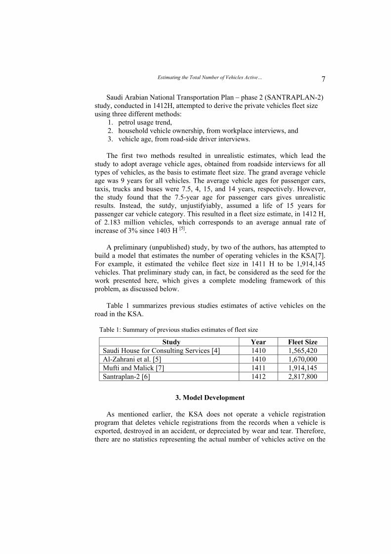
Table 1 summarizes previous studies estimates of active vehicles on the

road in the KSA.

Table 1: Summary of previous studies estimates of fleet size

3. Model Development

As mentioned earlier, the KSA does not operate a vehicle registration

program that deletes vehicle registrations from the records when a vehicle is exported, destroyed in an accident, or depreciated by wear and tear. Therefore, there are no statistics representing the actual number of vehicles active on the

Study Year Fleet Size Saudi House for Consulting Services [4] 1410 1,565,420 Al-Zahrani et al. [5] 1410 1,670,000 Mufti and Malick [7] 1411 1,914,145 Santraplan-2 [6] 1412 2,817,800


8

roads in the KSA, for any given year, except for the year 1403 H, when all vehicles were required to re-register.

In 1403 H, GTD re-issued license plates for all vehicles and kept a record

of the total number of vehicles reporting. That number of vehicles was, thus, considered to represent the actual vehicle fleet size operating in the KSA in year 1403 H. The size of that vehicle fleet was 2,163,925 vehicles. Thus, the vehicle fleet size in any year after 1403 H would be an estimate and not an exact figure. For this reason, a mathematical model is developed here to estimate the number of vehicles operating on the roads of the KSA, year by year. The model uses as its input the vehicle registration statistics shown in Figure 1, in addition to the statistics of vehicle exports and accidents, obtained from its sources.

The model estimates the number of vehicles leaving service each year due

to the three causes mentioned earlier, i.e.: 1. exported outside the KSA, 2. destroyed in accidents, or 3. retired when the useful life of the vehicle was

consumed due to use.

Thus, the total number of vehicles active on the road at any year t, TNVARt, is estimated according to the following mathematical model:

∑∑==

−−−==n

jjjjj

n

jjt NDNANXNRNOTNVAR

11)( (1)

where, NOj = actual number of vehicles of age j that are active on the road at year t. NRj = number of new registrations of vehicles of model j, assuming that all registration at any given year k are all of the same latest model. NXj = number of vehicles of age j exported outside KSA. NAj = number of vehicles of age j destroyed in traffic accidents. NDj = number of vehicles of age j depreciated due to wear and tear. j = the year when the vehicle was manufactured (model), or vehicle age; j = 1, 2, 3, . . . ; j = 1 is the most recent model. k = calendar year indicator, k = 1, 2, 3, . . .; t =1 is the most recent year. n = maximum vehicle age.

The general model’s three components, namely export, accident and decay sub-models, are discussed below.


9

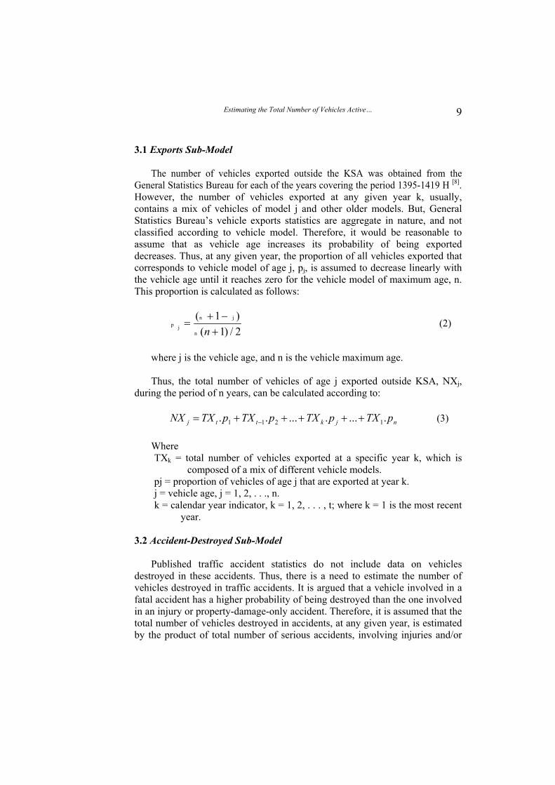
3.1 Exports Sub-Model

The number of vehicles exported outside the KSA was obtained from the General Statistics Bureau for each of the years covering the period 1395-1419 H [8]. However, the number of vehicles exported at any given year k, usually, contains a mix of vehicles of model j and other older models. But, General Statistics Bureau’s vehicle exports statistics are aggregate in nature, and not classified according to vehicle model. Therefore, it would be reasonable to assume that as vehicle age increases its probability of being exported decreases. Thus, at any given year, the proportion of all vehicles exported that corresponds to vehicle model of age j, pj, is assumed to decrease linearly with the vehicle age until it reaches zero for the vehicle model of maximum age, n. This proportion is calculated as follows:

2/)1()1(

+−+

=nn

jnp j (2)

where j is the vehicle age, and n is the vehicle maximum age. Thus, the total number of vehicles of age j exported outside KSA, NXj,

during the period of n years, can be calculated according to:

njkttj pTXpTXpTXpTXNX .......... 1211 +++++= − (3)

Where TXk = total number of vehicles exported at a specific year k, which is

composed of a mix of different vehicle models. pj = proportion of vehicles of age j that are exported at year k. j = vehicle age, j = 1, 2, . . ., n. k = calendar year indicator, k = 1, 2, . . . , t; where k = 1 is the most recent

year.

3.2 Accident-Destroyed Sub-Model

Published traffic accident statistics do not include data on vehicles destroyed in these accidents. Thus, there is a need to estimate the number of vehicles destroyed in traffic accidents. It is argued that a vehicle involved in a fatal accident has a higher probability of being destroyed than the one involved in an injury or property-damage-only accident. Therefore, it is assumed that the total number of vehicles destroyed in accidents, at any given year, is estimated by the product of total number of serious accidents, involving injuries and/or


10

fatalities, times the ratio of total fatalities to the sum of casualties (injuries and fatalities), at that year:

+

=kk

kkk InjFatal

FatalSerAccTA . (4)

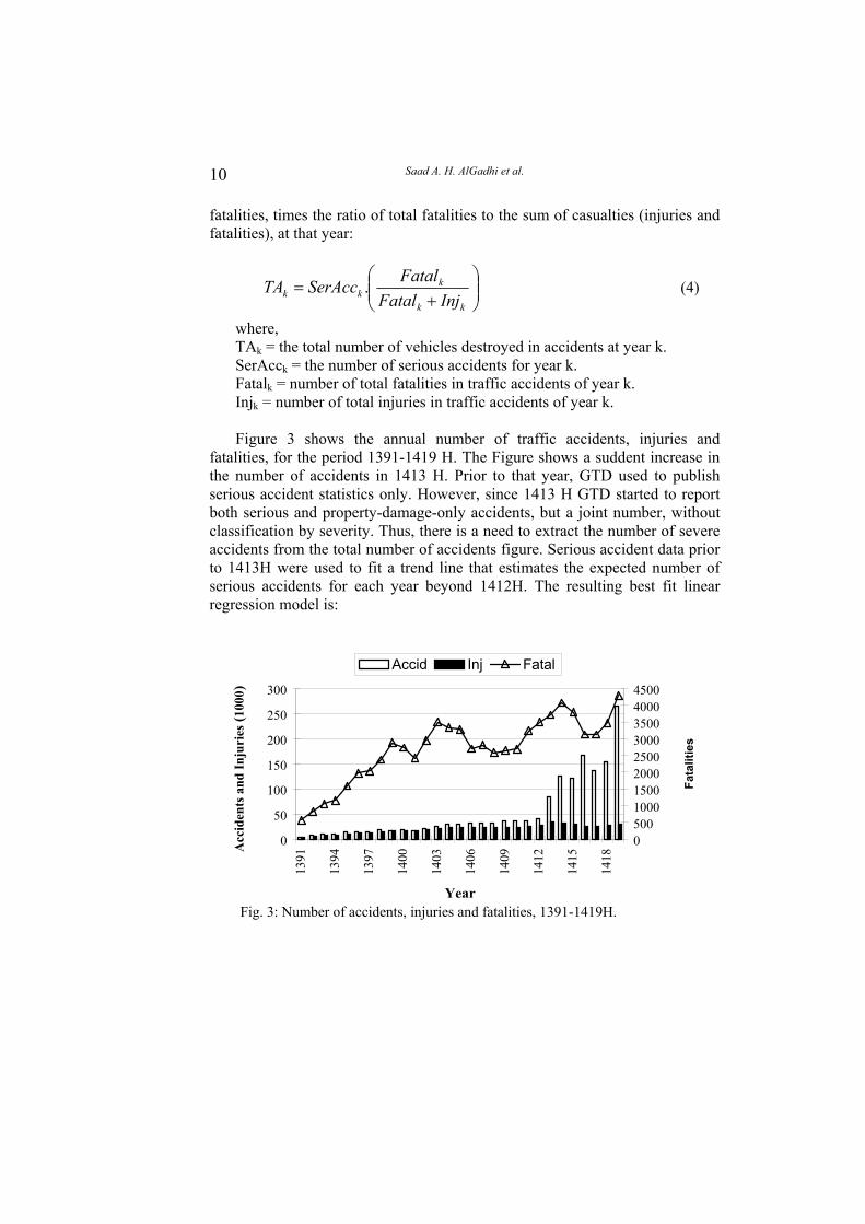
where, TAk = the total number of vehicles destroyed in accidents at year k. SerAcck = the number of serious accidents for year k. Fatalk = number of total fatalities in traffic accidents of year k. Injk = number of total injuries in traffic accidents of year k. Figure 3 shows the annual number of traffic accidents, injuries and

fatalities, for the period 1391-1419 H. The Figure shows a suddent increase in the number of accidents in 1413 H. Prior to that year, GTD used to publish serious accident statistics only. However, since 1413 H GTD started to report both serious and property-damage-only accidents, but a joint number, without classification by severity. Thus, there is a need to extract the number of severe accidents from the total number of accidents figure. Serious accident data prior to 1413H were used to fit a trend line that estimates the expected number of serious accidents for each year beyond 1412H. The resulting best fit linear regression model is:

0

50

100

150

200

250

300

1391

1394

1397

1400

1403

1406

1409

1412

1415

1418

Year

050010001500200025003000350040004500

Fata

litie

s

Accid Inj Fatal

Acc

iden

ts a

nd In

juri

es (1

000 )

Fig. 3: Number of accidents, injuries and fatalities, 1391-1419H.


11

kk YearSerAcc )(2.16193.2246623 +-= (5) n = 22, R2 = 0.99, where SerAcck is the number of serious accidents for year k, and (Year)k is

the digits of the corresponding Hijri calender year, e.g. 1395. On the other hand, the number of vehicles destroyed in accidents, at any

given year k, usually contains a mix of vehicles of model j and older models. Since the year of make (model) of vehicles involved in traffic accidents are not included in the accident statistics, it is assumed that the vehicle model proportions are, also, linearly decreasing with vehicle age, as represented by Eq. 2.

Thus, the total number of vehicles of model j destroyed in traffic accidents, NAj, during the period of n years, can be calculated according to:

njkttj pTApTApTApTANA .......... 1211 +++++= − (6)

where TAk is the total number of vehicles destroyed in accidents at a

specific year k, which is composed of a mix of different vehicle models.

3.3 Decay Sub-Model

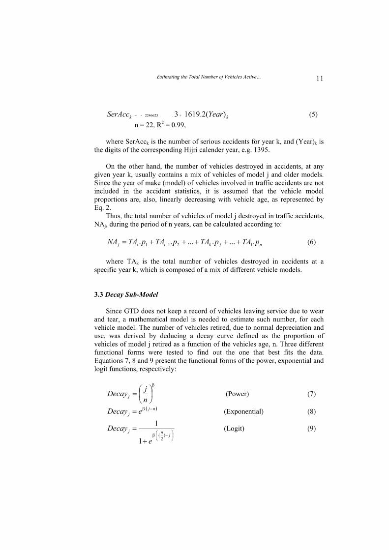
Since GTD does not keep a record of vehicles leaving service due to wear and tear, a mathematical model is needed to estimate such number, for each vehicle model. The number of vehicles retired, due to normal depreciation and use, was derived by deducing a decay curve defined as the proportion of vehicles of model j retired as a function of the vehicles age, n. Three different functional forms were tested to find out the one that best fits the data. Equations 7, 8 and 9 present the functional forms of the power, exponential and logit functions, respectively:

β

=

njDecay j (Power) (7)

( )njj eDecay −= β (Exponential) (8)

−

+

=jnj

e

Decay)

2(

1

1β

(Logit) (9)


12

where, Decayj = the proportion of vehicles of age j retiring. j = vehicle age; j = 1, 2, . . ., n. n = maximum vehicle age. β = calibration parameter. Figure 4 compares the graphs of the three functional forms for a

hypothetical 12-years maximum age, and using the corresponding calibrated values of β, as presented in the next section.

Each of the above three functions underlies a different vehicle deterioration

behavior. The depicted power function starts with a relatively low retirement proportion for new vehicles and, for β > 1, assumes a non-decreasing rate of increase in the proportion of vehicles retired as vehicle age increases. That is older vehicles deteriorate more rapidly than newer ones. The exponential function uses the same underlying assumption, except that, as vehicle ages, its rate of deterioration increases more rapidly than that given by the power function. In addition, it assumes the highest retirement proportion for new vehicles, i.e. at one-year age.

Finally, the logit function starts at a very low retirement proportion for new

vehicles, has flatter slopes for relatively new and very old vehicles, and has a very sharp rate of increase of vehicle deterioration proportion in between. Its use underlying assumption is that at very low vehicle ages, vehicles are still new and are, usually, under warranty. After the warranty expires the proportion of vehicle retirement increases at an increasing rate until vehicles pass their middle age. Vehicles passing the middle age threshold will show a decreasing rate of increase in retirement proportion, probably due to good maintenance, care and upkeep.

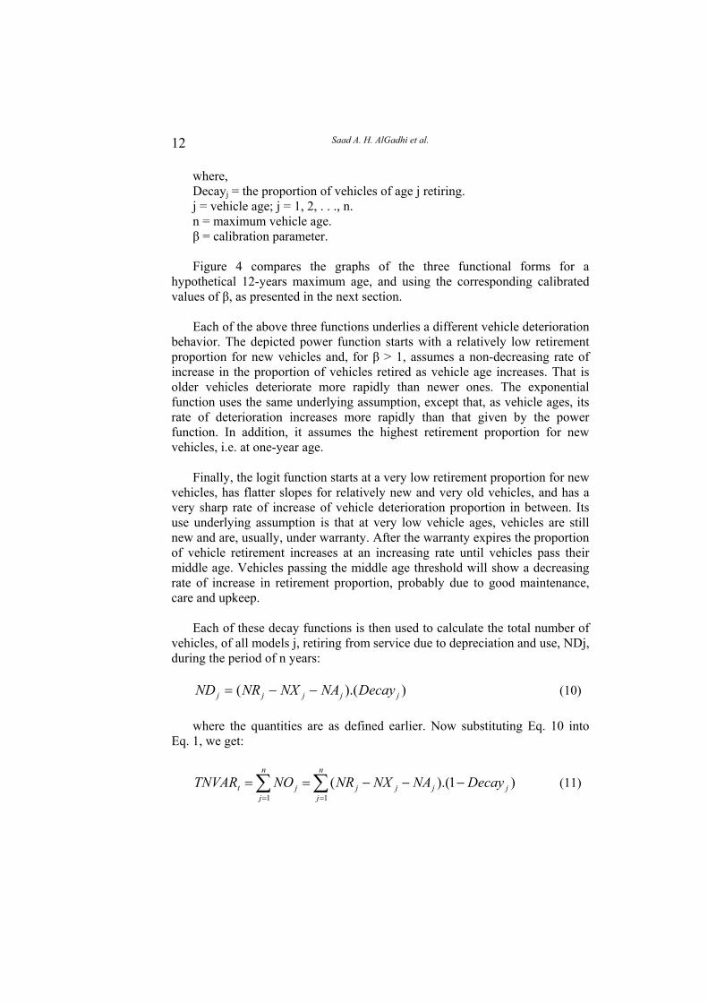
Each of these decay functions is then used to calculate the total number of

vehicles, of all models j, retiring from service due to depreciation and use, NDj, during the period of n years:

)).(( jjjjj DecayNANXNRND −−= (10)

where the quantities are as defined earlier. Now substituting Eq. 10 into

Eq. 1, we get:

)1).((11∑∑==

−−−==n

jjjjj

n

jjt DecayNANXNRNOTNVAR (11)


13

0.00.10.20.30.40.50.60.70.80.91.0

1 2 3 4 5 6 7 8 9 10 11 12

Age (Years)

Dec

ay P

ropo

rtio

n

PowerExponLogit

Combining Eq. 11, the two sub-models in Eq. 3 and Eq. 6, for exported vehicles of all models, NXj, and those destroyed in accidents, NAj, respectively, and each of the decay functions of Eqs. 7, 8 or 9, one can come up with three estimates of the total number of vehicles active on the road at any year k. Next section dicusses the calibration process of these three mathematical models and presents its results.

4. Model Calibration And Validation

The calibration process involves two steps. First, for each decay function

(Eqs. 7, 8 and 9), the calibration of its two parameters: the β parameter and the maximum vehicle life, n. Second, to select the best of the three calibrated decay function that fits data better.

The data used to calibrate the β parameter in the mathematical model of

Eq. 11, for each type of the three decay functions, include the following: 1. As stated earlier, GDT published in the 1403 H statistical summaries a

figure that is referred to as the “True Number” of all vehicles active on the road, i.e. TNVAR1403H. In that year, GDT required all vehicles, regardless of registration status, to re-register during that year. This effort produced a total vehicle count of 2,163,925 vehicles [3].

2. The total number of new registration of vehicles of model j , NRj. Such data is available from GTD published statistical reports [3].

Fig. 4: Comparison of power, exponential and logit decay functions


14

3. The number of vehicles exported outside KSA for each year, TXk. These are required, in Eq. 3, to estimate the number of vehicles of model j exported, NXj. This data was obtained from the General Statistics Bureau [8].

4. The total number of serious accidents (SerAcct), injuries (Injt), and fatalities (Fatalt) for each year. These are required, in Eqs. 4 and 6, to estimate the number of vehicles of model j destroyed in traffic accidents, NAj. This data is also available from GTD published statistical reports [3].

While the basic form of the decay functions was assumed, the β parameter

used to determine the exact shape of the curve was derived from real data. A spreadsheet computer program was designed and implemented to solve the mathematical model of Eq. 11, for different maximum vehicle ages and for each decay function type. The assumed maximum vehicle ages were started at 9 years, based on the results of a previous study that found that the average vehicle age in KSA was 9 years [6]. For each assumed maximum vehicle life, the program was run in an iterative fashion to find the value of the β parameter that yields a total vehicle count within 0.01% of the actual 1403 H vehicle count of 2,163,925.

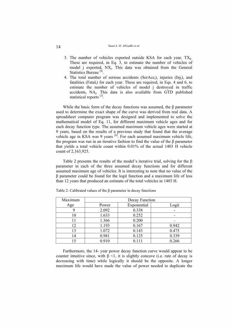
Table 2 presents the results of the model’s iterative trial, solving for the β

parameter in each of the three assumed decay functions and for different assumed maximum age of vehicles. It is interesting to note that no value of the β parameter could be found for the logit function and a maximum life of less than 12 years that produced an estimate of the total vehicles in 1403 H. Table 2: Calibrated values of the β parameter in decay functions

Decay Function Maximum

Age Power Exponential Logit 9 2.092 0.338 -

10 1.633 0.252 - 11 1.366 0.200 - 12 1.193 0.167 0.942 13 1.072 0.143 0.475 14 0.981 0.125 0.339 15 0.910 0.111 0.266

Furthermore, the 14- year power decay function curve would appear to be

counter intuitive since, with β <1, it is slightly concave (i.e. rate of decay is decreasing with time) while logically it should be the opposite. A longer maximum life would have made the value of power needed to duplicate the


15

1403 H data even smaller, as for the 15-year power function, the decay curve more concave, and the result more counter intuitive.

Since each of the maximum vehicle ages shown in Table 2, for each of the

three decay functions, satisfied the condition of using the new vehicle registration data to estimate the 2,163,925 vehicles in the KSA on 1403 H, a second validity test is used to select the best of these ages, for each decay function. This second test compares the proportion of retired vehicles by model (year of make) as estimated by Eq. 11, for each maximum life, and the corresponding proportion of non-inspected vehicles as observed from data collected by the MVIP in 1410 H.

The MVIP data of inspected vehicles in 1410H, by age, were reported in

the Al- Zahrani et al. study [5]. The MVIP program inspected in 1410H a very large number of vehicles in the KSA and collected statistics on the age of the vehicle at the time of inspection. While the total number of vehicles inspected may not be the total of all vehicles in the KSA, the large sample (approximately 1 million vehicles) would create a fairly accurate statistics on the mix of vehicle ages.

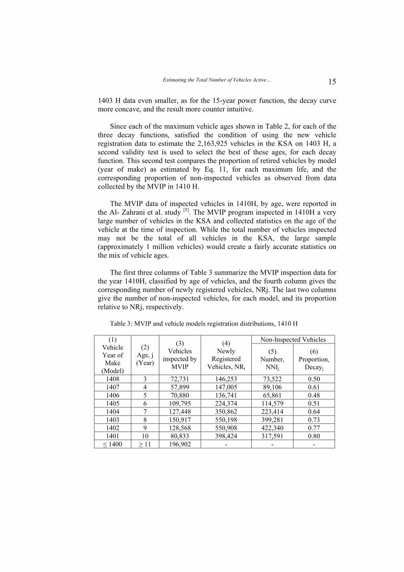
The first three columns of Table 3 summarize the MVIP inspection data for

the year 1410H, classified by age of vehicles, and the fourth column gives the corresponding number of newly registered vehicles, NRj. The last two columns give the number of non-inspected vehicles, for each model, and its proportion relative to NRj, respectively.

Table 3: MVIP and vehicle models registration distributions, 1410 H

Non-Inspected Vehicles (1) Vehicle Year of Make

(Model)

(2) Age, j (Year)

(3) Vehicles

inspected by MVIP

(4) Newly

Registered Vehicles, NRt

(5) Number,

NNIj

(6) Proportion,

Decayj

1408 3 72,731 146,253 73,522 0.50 1407 4 57,899 147,005 89,106 0.61 1406 5 70,880 136,741 65,861 0.48 1405 6 109,795 224,374 114,579 0.51 1404 7 127,448 350,862 223,414 0.64 1403 8 150,917 550,198 399,281 0.73 1402 9 128,568 550,908 422,340 0.77 1401 10 80,833 398,424 317,591 0.80 ≤ 1400 ≥ 11 196,902 - - -


16

By invoking Eq. 10, the proportion of vehicles retired for each vehicle model of age j, Decayj, would be obtained as follows:

)( jjjjj NANXNRNDDecay −−= (12)

However, the NDj, NXj, and NAj quantities are unknown apriori; the only

known quantity is NRj. If the MVIP inspection data is complete with respect to KSA area coverage

and vehicle inspection compliance, the number of vehicles that were not inspected (NNIj) would consist of vehicles that have been exported, NXj, destroyed in accidents, NAj, and depreciated by wear and tear, NDj, i.e. NNIj = (NXj + NAj + NDj). But Al-Zahrani et al. [5] show that MVIP inspection data is not complete regarding coverage and compliance. Thus, Decayj can be approximated by dividing the total number of vehicles that did not show-up for inspection, for each vehicle model of age j, NNIj, by number of the registered number of this type of vehicle, NRj; i.e., jjj NRNNIDecay /= . Last column of Table 3 shows the Decayj for each vehicle model, as calculated by this alternative method.

As shown in the Table, proportion of vehicles retiring from service due to

aging shows an increasing trend for vehicle models older than 4 years (j > 4). Decay proportions for vehicle models of age 3 and 4 years seem illogical. This might be due to the fact that new vehicles in KSA are exempted, by law, from compulsory inspection during its first 3 years and, as discussed earlier, that newer vehicle models have higher probabilities of being exported and/or destroyed in traffic accidents, see Eq. 2. Therefore, the Decay proportions for these two age classes are excluded from further consideration.

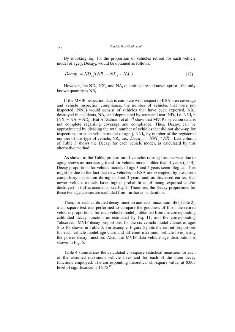
Then, for each calibrated decay function and each maximum life (Table 2),

a chi-square test was performed to compare the goodness of fit of the retired vehicles proportions, for each vehicle model j, obtained from the corresponding calibrated decay function as estimated by Eq. 11, and the corresponding “observed” MVIP decay proportions, for the six vehicle model classes of ages 5 to 10, shown in Table 3. For example, Figure 5 plots the retired proportions for each vehicle model age class and different maximum vehicle lives, using the power decay function. Also, the MVIP data vehicle age distribution is shown in Fig. 5.

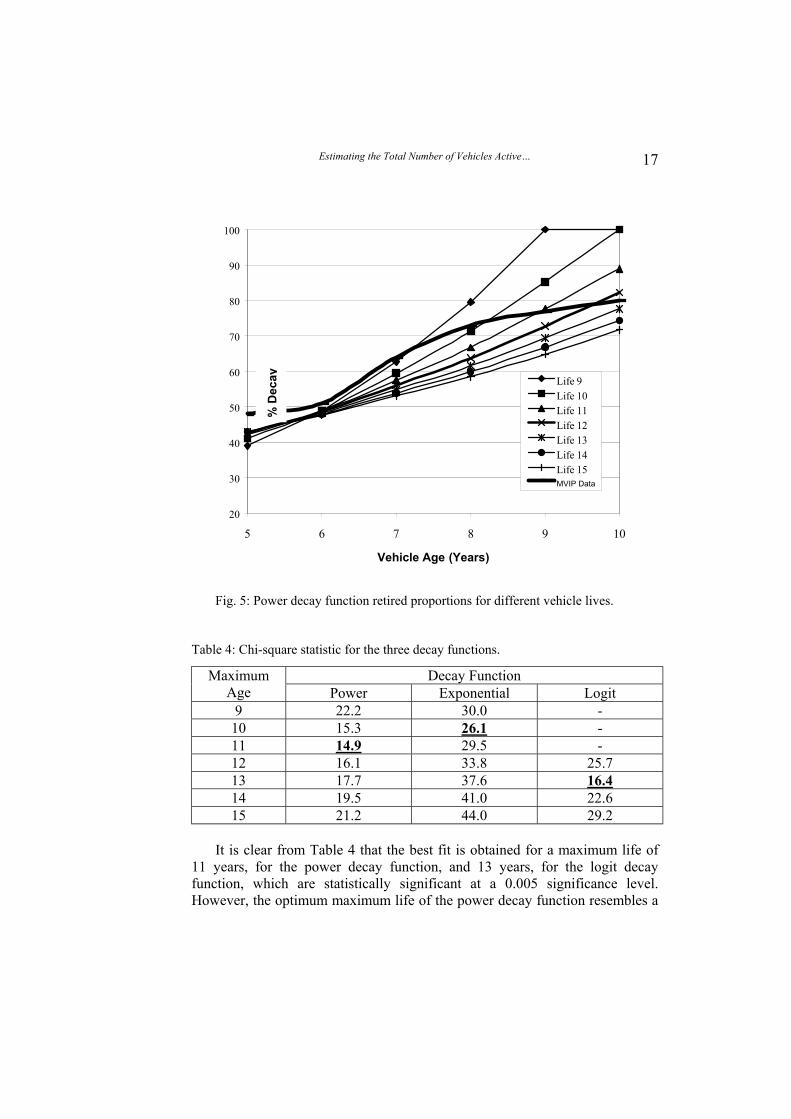
Table 4 summarizes the calculated chi-square statistical measures for each

of the assumed maximum vehicle lives and for each of the three decay functions employed. The corresponding theoretical chi-square value, at 0.005 level of significance, is 16.75 [9].


17

20

30

40

50

60

70

80

90

100

5 6 7 8 9 10

Vehicle Age (Years)

Life 9Life 10Life 11Life 12Life 13Life 14Life 15MVIP Data

Fig. 5: Power decay function retired proportions for different vehicle lives.

Table 4: Chi-square statistic for the three decay functions.

Decay Function Maximum Age Power Exponential Logit

9 22.2 30.0 - 10 15.3 26.1 - 11 14.9 29.5 - 12 16.1 33.8 25.7 13 17.7 37.6 16.4 14 19.5 41.0 22.6 15 21.2 44.0 29.2

It is clear from Table 4 that the best fit is obtained for a maximum life of

11 years, for the power decay function, and 13 years, for the logit decay function, which are statistically significant at a 0.005 significance level. However, the optimum maximum life of the power decay function resembles a

% D

ecay


18

better fit than that of the logit decay function. For the exponential decay function, the lowest chi-square value is obtained at 10-year maximum life, but it was not statistically significant.

Therefore, it can be concluded that the mathematical model of Eq. 11 that

utilizes the power decay function and a 11-year maximum vehicle life yields an estimate that best compares with the MVIP statistics, since the value of the chi-squared measure is at a minimum (best fit) for this value. A zero value of chi-square measure would be a perfect fit [9].

In order to validate the calibrated power function model it would be

appropriate to compare its estimate of the total number of vehicles active on the road at this year (1421H), TNVAR1421H, with the actual number of vehicles on the road in the same year. In 1417H, GTD started to issue new (alpha-numerical) license plates, for new vehicle registrations only. A year later, GTD began to gradually replace the old numerical license plates with the new alphanumerical ones upon the renewal of its licenses, for all vehicles in the KSA,. By now all vehicles active on the road should, by law, have new license plates. GTD is keeping record of all the new alphanumerical license plates issued. GTD is expected to officially release this figure, which should represent the best available estimate of the actual number of vehicles on the road in KSA in 1421 H.

However, the calibrated power function model was used to predict the total

number of vehicles active on the road for the year 1419 H, TNVAR1419H, since it was the latest year having published statistics on vehicle exports and traffic accidents; the calibrated model estimates that the number of operating vehicles for the year 1419 H would have been 1,783,377 vehicles.

Unofficial statistics obtained from the Ministry of Interior Information

Center suggest that the total number of vehicles that have received the new alphanumerical license plates until 15/08/1421 H was 3,322,160 vehicles. Thus, the number of vehicles entering service during all of year 1420 H and most (8.5 months) of 1421 H should be removed from this figure, to be comparable with the power function model estimate at the end of year 1419 H. Furthermore, some of the vehicles included in the last figure would have been no longer active on the road because they were exported, destroyed in accidents or retired. The vehicles leaving service during the years 1417-21 H, due to any of the three write-off reasons, were removed from the above figure. This total number of vehicles leaving service was estimated to be 195,040 vehicles, by using Eqs. 3, 6 and 10.


19

Therefore, the resulting “actual” number of vehicles on the road at the end of year 1419 H would most probably have been 2,111,614 vehicles, which deviates from the corresponding calibrated power function model estimated number by about 15.5%. This can be considered as an acceptable validation of the calibrated mathematical model, given the suspected overcounting of vehicles receiving new alphanumerical license plates; It is not clear if the 1421 H true number, reported by the Ministry of Interior Information Center, includes double counting of vehicles receiving replacement license plates for their lost or damaged ones.

5. Model Application

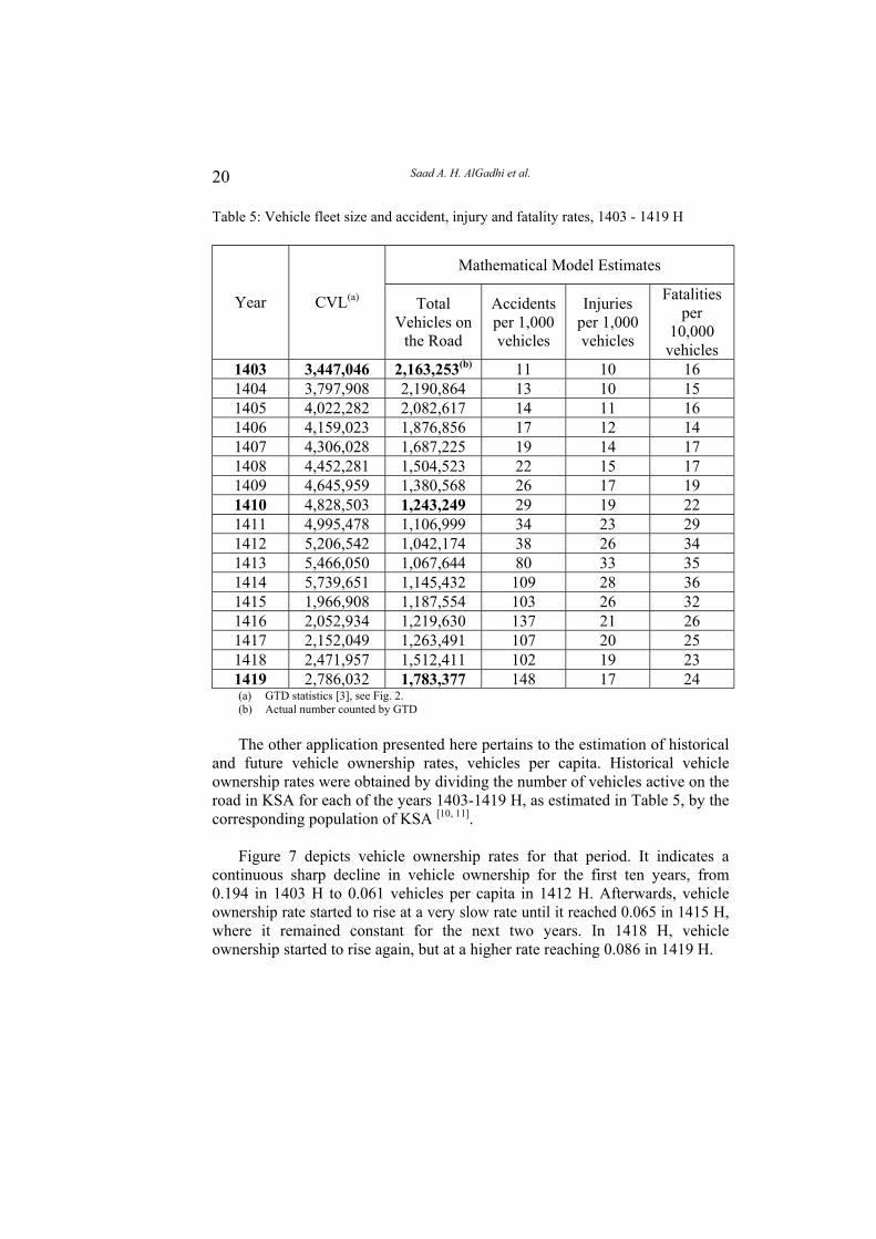
With 11-years maximum vehicle life, the calibrated and validated power function mathematical model is now used to demonstrate some of the potential applications of the estimated total number of vehicles active on the road at any given year. The first application is to develop accident and injury rates, per 1000 vehicles, and fatalities rates, per 10,000 vehicles, in the KSA. The model is first applied to the years 1403 - 1419 H to produce an estimate of the vehicle fleet size for each year. Annual accident statistics for that period were obtained from the GDT publication [3].

Table 5 shows the resulting vehicle fleet sizes estimated by the mathematical model, along with the corresponding CVL figures, published by GTD, where it is clear that the CVL figures overestimate the actual vehicle fleet sizes. Furthermore, the fleet size estimated for year 1410 H, i.e. 1,243,249 vehicles, shows that the percentage of vehicles not reporting to MVIP stations is only 25%, as compared to the 67% assumed by Al-Zahrani et al. [5].

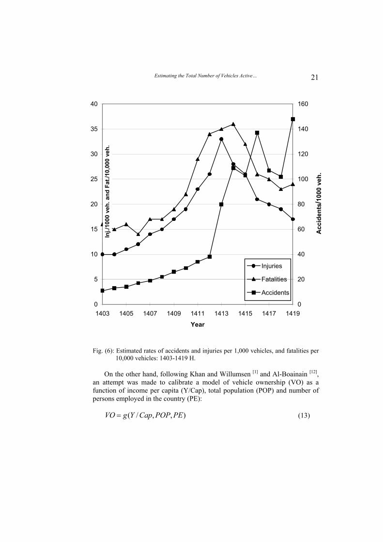
The Table also details the corresponding accident, injury and fatality rates.

These rates are depicted in Figure 6. It should be noted that prior to 1413 H, property-damage-only accidents used to be omitted from GTD accident statistics. Afterwards, GTD started to report them. This explains the sudden rise in the accident numbers (Fig. 3) and accident rates (Fig.6) after 1412 H.

Table 5 and Figure 6 indicate that the rate of accidents and fatalities has begun to rise again in the KSA. This, however, might be explained by a likely rise in vehicle kilometers traveled by each vehicle. The vehicle kilometers traveled data is not available at this time. On the other hand, the slight reduction in injury rates should not be seen as an absolute positive sign since it is accompanied by a slight increase in fatality rate. This might suggest that serious accidents are getting to be more fatal.


20

Table 5: Vehicle fleet size and accident, injury and fatality rates, 1403 - 1419 H

Mathematical Model Estimates

Year CVL(a) Total Vehicles on

the Road

Accidents per 1,000 vehicles

Injuries per 1,000 vehicles

Fatalities per

10,000 vehicles

1403 3,447,046 2,163,253(b) 11 10 16 1404 3,797,908 2,190,864 13 10 15 1405 4,022,282 2,082,617 14 11 16 1406 4,159,023 1,876,856 17 12 14 1407 4,306,028 1,687,225 19 14 17 1408 4,452,281 1,504,523 22 15 17 1409 4,645,959 1,380,568 26 17 19 1410 4,828,503 1,243,249 29 19 22 1411 4,995,478 1,106,999 34 23 29 1412 5,206,542 1,042,174 38 26 34 1413 5,466,050 1,067,644 80 33 35 1414 5,739,651 1,145,432 109 28 36 1415 1,966,908 1,187,554 103 26 32 1416 2,052,934 1,219,630 137 21 26 1417 2,152,049 1,263,491 107 20 25 1418 2,471,957 1,512,411 102 19 23 1419 2,786,032 1,783,377 148 17 24 (a) GTD statistics [3], see Fig. 2. (b) Actual number counted by GTD The other application presented here pertains to the estimation of historical

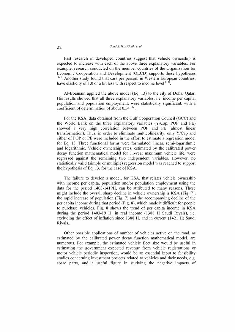
and future vehicle ownership rates, vehicles per capita. Historical vehicle ownership rates were obtained by dividing the number of vehicles active on the road in KSA for each of the years 1403-1419 H, as estimated in Table 5, by the corresponding population of KSA [10, 11].

Figure 7 depicts vehicle ownership rates for that period. It indicates a

continuous sharp decline in vehicle ownership for the first ten years, from 0.194 in 1403 H to 0.061 vehicles per capita in 1412 H. Afterwards, vehicle ownership rate started to rise at a very slow rate until it reached 0.065 in 1415 H, where it remained constant for the next two years. In 1418 H, vehicle ownership started to rise again, but at a higher rate reaching 0.086 in 1419 H.


21

0

5

10

15

20

25

30

35

40

1403 1405 1407 1409 1411 1413 1415 1417 1419

Year

0

20

40

60

80

100

120

140

160

Acc

iden

ts/ 1

000

veh.

Injuries

Fatalities

Accidents

Fig. (6): Estimated rates of accidents and injuries per 1,000 vehicles, and fatalities per

10,000 vehicles: 1403-1419 H. On the other hand, following Khan and Willumsen [1] and Al-Boainain [12],

an attempt was made to calibrate a model of vehicle ownership (VO) as a function of income per capita (Y/Cap), total population (POP) and number of persons employed in the country (PE):

),,/( PEPOPCapYgVO = (13)

Inj./

1000

veh

. and

Fat

./10,

000

veh.


22

Past research in developed countries suggest that vehicle ownership is expected to increase with each of the above three explanatory variables. For example, research conducted on the member countries of the Organization for Economic Cooperation and Development (OECD) supports these hypotheses [13]. Another study found that cars per person, in Western European countries, have elasticity of 1.0 or a bit less with respect to income level [14].

Al-Boainain applied the above model (Eq. 13) to the city of Doha, Qatar.

His results showed that all three explanatory variables, i.e. income per capita, population and population employment, were statistically significant, with a coefficient of determination of about 0.54 [12].

For the KSA, data obtained from the Gulf Cooperation Council (GCC) and

the World Bank on the three explanatory variables (Y/Cap, POP and PE) showed a very high correlation between POP and PE (almost linear transformation). Thus, in order to eliminate multicolinearity, only Y/Cap and either of POP or PE were included in the effort to estimate a regression model for Eq. 13. Three functional forms were formulated: linear, semi-logarithmic and logarithmic. Vehicle ownership rates, estimated by the calibrated power decay function mathematical model for 11-year maximum vehicle life, were regressed against the remaining two independent variables. However, no statistically valid (simple or multiple) regression model was reached to support the hypothesis of Eq. 13, for the case of KSA.

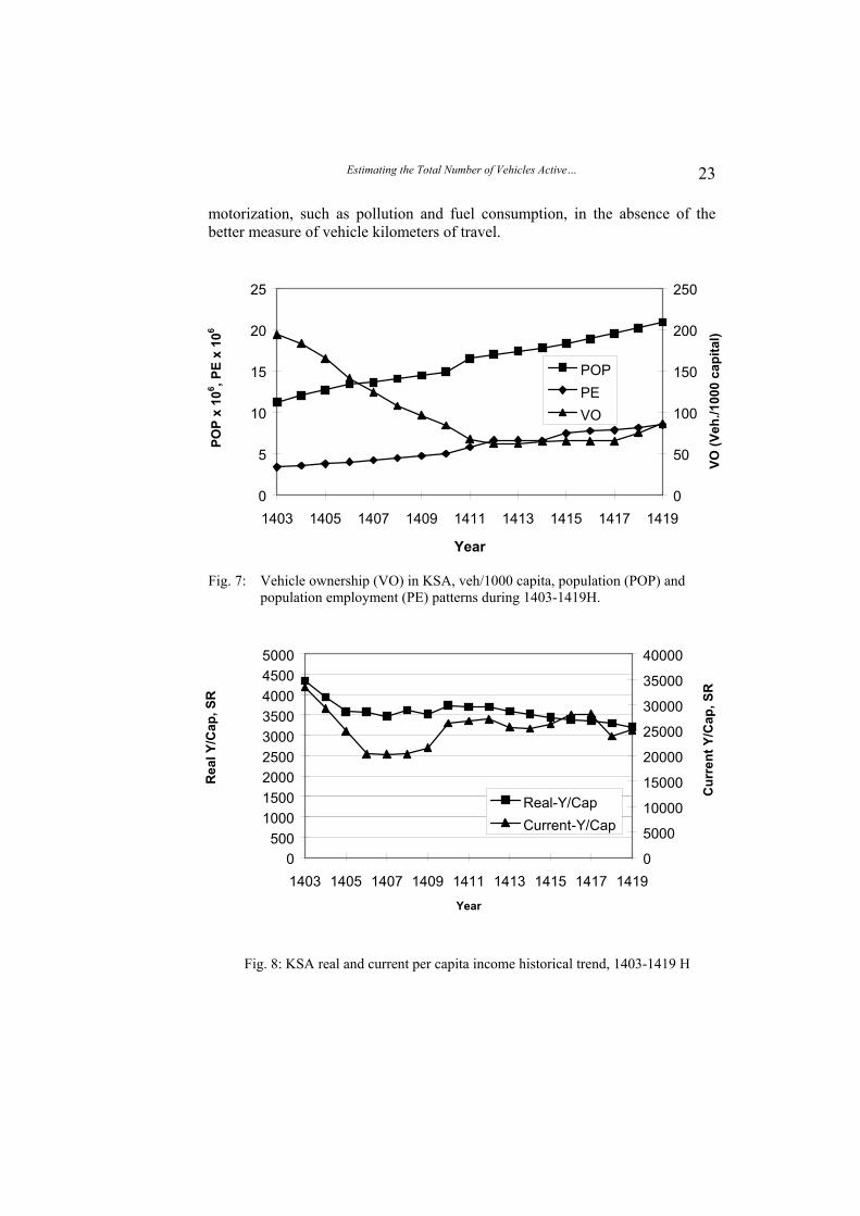
The failure to develop a model, for KSA, that relates vehicle ownership

with income per capita, population and/or population employment using the data for the period 1403-1419H, can be attributed to many reasons. These might include the overall sharp decline in vehicle ownership is KSA (Fig. 7), the rapid increase of population (Fig. 7) and the accompanying decline of the per capita income during that period (Fig. 8), which made it difficult for people to purchase vehicles. Fig. 8 shows the trend of per capita income in KSA during the period 1403-19 H, in real income (1388 H Saudi Riyals), i.e. excluding the effect of inflation since 1388 H, and in current (1421 H) Saudi Riyals,.

Other possible applications of number of vehicles active on the road, as

estimated by the calibrated power decay function mathematical model, are numerous. For example, the estimated vehicle fleet size would be useful in estimating the government expected revenue from vehicle registrations or motor vehicle periodic inspection, would be an essential input to feasibility studies concerning investment projects related to vehicles and their needs, e.g. spare parts, and a useful figure in studying the negative impacts of


23

Rea

l Y/C

ap, S

R

motorization, such as pollution and fuel consumption, in the absence of the better measure of vehicle kilometers of travel.

0

5

10

15

20

25

1403 1405 1407 1409 1411 1413 1415 1417 1419

Year

0

50

100

150

200

250

POPPEVO

Fig. 7: Vehicle ownership (VO) in KSA, veh/1000 capita, population (POP) and population employment (PE) patterns during 1403-1419H.

0500

100015002000250030003500400045005000

1403 1405 1407 1409 1411 1413 1415 1417 1419Year

0

5000

10000

15000

20000

25000

30000

35000

40000

Real-Y/CapCurrent-Y/Cap

Fig. 8: KSA real and current per capita income historical trend, 1403-1419 H

POP

x 10

6 , PE

x 10

6

VO (V

eh./1

000

capi

tal)

Cur

rent

Y/C

ap, S

R


24

6. Conclusions

The aim of this paper have been to present the effort of developing a mathematical model that yields a more likely estimate of the total number of vehicles active on the road in KSA, than does the officially reported cumulative vehicle license (CVL) number, and to demonstrate some of its potential applications. The study reached the following conclusions: • Review of past research revealed that there has been no reliable

source and/or method to estimate the most likely number of vehicles active on the road in the Kingdom of Saudi Arabia (KSA). Such figure is, no doubt, essential in the road infrastructure planning and management.

• Vehicle registration record system, in the KSA, lacks a program that writes off vehicles leaving service due to being exported outside the KSA, destroyed in accidents and/or depreciated by wear and tear.

• The current CVL statistic, published annually by the General Traffic Directorate (GTD), overestimates the most likely number of vehicles active on the road. Current CVL is calculated as the sum of newly registered vehicles during the latest past 10-year rolling time frame.

• The mathematical model developed here, which accounts for all three sources of leakage of vehicles from the CVL statistics, appears to be robust in the following sense: a. Its estimate of the number of vehicles on the road in

1403H (2,163,253 vehicles) matches the actual number reported by GTD, when it asked all vehicles to re-register,

b. Its predictions of vehicle mix age distribution in 1410 H is statistically indifferent from that observed in MVIP data,

c. Its prediction of the fleet size in 1419H (1,783,377 vehicles) closely matches the recently reported number of (the new) alphanumerical license plates issued to all vehicles in the KSA.

• It appears that the most probable average maximum vehicle age in the KSA is 11 years. This figure is within the range of 5 to 11 years, expected for passenger cars in the study of the Saudi House for Consulting Services [4], and close to the average vehicle age, for all types of vehicles, observed by SANTRAPLAN-2 study [6].

• The calibrated mathematical model shows that vehicle decay curve, due to aging, is best represented by a non-concave power decay


25

function. That is a non-decreasing rate of increase in the proportion of vehicles retired as vehicle age increases.

• Application of the calibrated model estimates of vehicle fleet to study the historical trend of traffic accidents and its severity indicate that the rate, per 1000 vehicles, of accidents and fatalities has begun, in 1419 H, to rise in the KSA. This warrants further study and analysis of its causes and required countermeasures.

• Vehicle ownership rates in the KSA have shown a sharp decline for the ten years period of 1403 H to 1412 H, from 0.194 to 0.061 veh/capita, respectively. The rate started to increase gradually since then, to reach 0.086 veh/capita in 1419 H.

• To provide an instrument to forecast future vehicle ownership, the study attempted to calibrate a model of vehicle ownership (VO) as a function of income per capita (Y/Cap), total population (POP) and number of persons employed in the country (PE). However, no statistically valid (simple or multiple) regression model was reached. This appears to be due to the abnormal conditions that prevailed in the KSA during the period of analysis (1403-1419 H). These include overall sharp decline in vehicle ownership, the rapid increase of population and the accompanying decline of the per capita income during that period. Of course, to have an ideal and accurate source of the number of vehicles

active on the road, GTD should establish a program that deletes vehicles leaving service for any reason, either temporarily or permanently, from its vehicle registry system. However, until this is done it is recommended that the mathematical model developed here is employed to continuously provide this essential figure, which has many applications, some of which were demonstrated in this paper. On the other hand, it is recommended that a separate study be undertaken to develop a policy-sensitive model of vehicle ownership that predicts future vehicle ownership as a function of factors such as fuel price per liter, vehicle import customs tariff, and the associated annual ownership or registration fee.

Acknowledgement: The authors would like to acknowledge the support

and help provided by Engineer Saad A. Al-Samnan for helping in collecting the data used in this study.

References

[1] Khan, Amer and Luis G. Willumsen, “Modelling Car Ownership and Use

in Developing Countries,” Traffic Engineering and Control, November 1986, pp. 554-560.


26

[2] Ortuzar, J. D. and L. G. Willumsen. Modelling Transport. Second edition, Wiley, 1994.

[3] The General Directorate of Traffic, Vehicle and Accident Statistical Report, different issues

[4] Riyadh Daily Newspaper, Number of automobiles likely to drop. Vol. VI, No. 74, p. 2, Riyadh, Monday, July 30, 1990.

[5] Al-Zahrani, A. H., H. D. Al-Bar and A. S. Al-Mahnabi, “An Analysis of Data on the Motor Vehicle Inspection Program in Saudi Arabia,” Proceedings of the Third Saudi Engineering Conference, King Saud University, V. 1, pp. 233-239, Riyadh, 1412 H.

[6] Ministry of Planning, “Saudi Arabian National Transportation Plan, SANTRAPLAN-2,’ GTZ Consultants, Riyadh, 1992.

[7] Mufti, Rasin K. and Daniel F. Malick, “Estimating the number of vehicles on the road in the Kingdom of Saudi Arabia,” working paper, Ministry of Communications, Saudi Arabia, Rajab 1412H (January 1992).

[8] General Statistics Bureau, Foreign Trade Statistics, Ministry of Planning, different editions.

[9] Hamburg, Morris. Statistical Analysis for Decision-making. Harcourt, Brace and World, 1970.

[10] World Bank, World Statistical Summaries, 1999. [11] Gulf Cooperation Council, “Economic Bulletin,” Volume XIV, 1999. [12] Al-Boainain, Abdulrahman Ali, “The analysis of urban road traffic flow

in the city of Doha,” Ph. D. Dissertation, Rensselar Polytechnic Institute, 1988.

[13] OECD, “Car Ownership and Use,” Organization for Economic Cooperation and Development (OECD), Road Transport Research Programme, Paris, 1982.

[14] Horn, Matthews and D. Symmes, “Assessing Present Car Ownership and Future Prospects,” ITE Journal, March 1985, pp. 26-32.


27

تقدير عدد المركبات العاملة على الطرق في المملكة العربية السعودية

**، و دانيال مالك**، رصين قدري المفتي*سعد عبدالرحمن القاضي

،800. ب.أستاذ مشارك، قسم الهندسة المدنية، جامعة الملك سعود، ص* .، المملكة العربية السعودية11421الرياض

. السعوديةواصالت، الرياض، المملكة العربيةخبير نقل سابق، وزارة الم**

تعد معرفة حجم أسطول المركبات العاملة على الطرق : المستخلص ونظراً ألن الحجـم . مدخال هاما لتخطيط وإدارة النقل على الطرق

الفعلي لألسطول في المملكة العربية السعودية غير معروف، فـإن علـى النمذجـة الرياضـية هذه الورقة العلمية تقدم منهجية مستندة

ويتكون النموذج الرياضي مـن ثالثـة . لتقدير حجم هذا األسطول نماذج جزئية تقوم بتقدير عدد المركبات التي تخرج مـن الخدمـة بسبب تصديرها للخارج، أو لتلفها في حوادث مرورية، أو لتقـادم

وتتكون مدخالت النموذج من اإلحصـائيات . عمرها، على الترتيب المتوافرة عن إصدارات رخص المركبات الجديدة، وتصدير السنوية

وقد تم اختبار ثالث دوال مختلفـة . المركبات، والحوادث المرورية لنموذج تقادم عمر المركبات، هي الدالة المرفوعة لقـوة، والدالـة

وقد تمت معايرة النموذج الرياضي باستخدام ". لوجت"األسية، ودالة هـ، عندما تم استدعاء جميـع 1403م حجم األسطول الفعلي في عا

المركبات إلعادة التسجيل، وكذلك توزيع أعمـار المركبـات لعـام . هـ، من واقع بيانات محطات الفحص الـدوري للمركبـات 1410

وتبين نتائج المعايرة أن الدالة المرفوعة لقوة أعطت أفضل نمـوذج رياضي، من الناحية اإلحصائية، وأن متوسط العمـر االفتراضـي

وبعد معايرة النموذج تم ترسـيخه . سنة 11للمركبات بالمملكة هو


28

1.8حـوالي (هــ 1419من خالل مقارنة تقديره لألسطول عـام مع العدد الفعلي للمركبات التـي حصـلت علـى لوحـات ) مليون

وتعرض الورقـة مثـالين لتطبيقـات النمـوذج . الحروف الجديدة ـ ل التسلسـل الزمنـي الرياضي، بعد معايرته وترسيخه، هما تحلي

1000التجاهات معدالت الحوادث واإلصـابات والوفيـات، لكـل مركبة، واتجاهات ملكية المركبات، لكل شخص، في المملكة العربية

.السعودية

estimating the total number of vehicles active on the road in saudi …€¦ · ·...

Documents