estimating the elasticity of trade - lem
TRANSCRIPT


Estimating the elasticity of trade:
the trade share approach
Mauro Lanati ∗
March 2013, revised April 2013
Abstract
Recent theoretical work on international trade emphasizes the importance
of trade elasticity as the fundamental statistic needed to conduct welfare
analysis. Eaton and Kortum (2002) proposed a two-step method to esti-
mate this parameter, where exporter fixed effects are regressed on proxies
for technology and wages. Within the same Ricardian model of trade, the
trade share provides an alternative source of identication for the elasticity of
trade. Following Santos Silva and Tenreyro (2006) both trade share and EK
models are estimated using OLS and Poisson PML to test for the presence of
heteroskedasticity-type-of-bias. The evidence from both specifications sug-
gests that the bias in the OLS estimates significantly impacts the magnitude
of trade cost elasticity. The welfare analysis reveals that the resulting ex-
treme variability of the trade cost elasticity and the imposition of a common
manufacturing share parameter for all countries generate substantial distor-
tions in the calculation of benefits from trade.
JEL: F10, F11, F14
Keywords: trade cost elasticity; gravity model; competitiveness equation;
trade share; gains from international trade
∗Department of Economics and Management, University of Pisa. Email: mauro.lanati@
for.unipi.it. I am especially grateful to Prof. Keith Head for helpful comments and sugges-
tions and to the SBE division of Sauder Business School for hosting me. I thank Prof.Fagiolo
(Sant’Anna School of Advanced Studies) and Prof.De Benedictis (University of Macerata) for
useful suggestions.
1

1 Introduction
The elasticity of trade is a parameter which plays a key role in calculating the wel-
fare gains from trade. Arkolakis et al. (2012) showed that within a particular class
of trade models, the elasticity of trade and the share of expenditure on domestic
goods are the only two parameters needed to calculate welfare gains from trade.1
Since the import ratio is directly observable from the data, the estimation of the
elasticity of trade becomes the key statistics for conducting welfare analysis.
The influential Eaton and Kortum (2002) article (henceforth EK) provides three
different ways to estimate the elasticity of trade θ , all derived from their Ricar-
dian model of trade. The first method estimates θ by relating trade variation to a
proxy for trade costs. As proxy for bilateral trade frictions they use the maximum
price difference across goods between countries. This one-step methodology is
based on a strong assumption: the price differences cannot be larger than trade
costs. A method of moments estimator gives an elasticity of 8.28, which is the EK
benchmark for welfare analysis.
The same proxy for trade costs has been used by EK in a second method for
estimating θ . This is again a one-step methodology where a transformed version
of bilateral trade is regressed on the proxy of trade costs, importer and exporter
fixed effects. In this alternative specification the proxy coefficient gives a measure
of the elasticity of trade parameter. The geographic terms are used as instruments
for the trade costs variable in a 2SLS analysis: they obtain an elasticity of 12.86.
Simonovska and Waugh (2011) showed that these two methods lead to upward
biased estimates of the elasticity of trade. To correct for this bias they propose a
new simulated method of moments estimator. They apply their estimator to dis-
aggregate price and trade-flow data for the year 2004. Their benchmark estimate
for θ is 4.12, a measure which is less than a half of EK’s preferred estimation.
1The trade models to which Arkolakis et al. conclusions apply are those models which feature
the following assumptions: a) Dixit-Stieglitz preferences; b) one factor of production; c) linear cost
functions; d) perfect or monopolistic competition along with three macro level restrictions i) trade
is balanced; ii) aggregate profits are a constant share of aggregate revenues; and iii) the import
demand system is CES. Among these models there are (besides the Armington model) Eaton and
Kortum (2002), Krugman (1980) and variations and extensions of Melitz (2003) featuring pareto
distributions of firm-level productivity.
2

The third methodology to estimate trade elasticity employed in EK is a grav-
ity based two-step procedure. EK provide a version of trade equation where
a transformed bilateral trade variable is regressed on exporter technology and
wages: they modify their original trade share expression until the price of inter-
mediaries pi disappears from the final two-step equation. In this competitiveness
equation the wage coefficient gives exactly a measure of the elasticity of trade
µw = µt = −θ . By instrumenting for wages their estimates yield an elasticity of
3.60. Simonovska and Waugh (2011) view this last EK estimate as reliable, since
3.60 is in line with their benchmark result.
Within the same EK Ricardian model of trade the original trade share expression
can be viewed as an alternative competitiveness equation, in which bilateral im-
ports are function of prices other than technology, wages and geographic barriers.
As Head and Mayer (2013) pointed out, the key difference is that in the trade
share expression the wage elasticity is µw = −βθ whereas the trade elasticity is
µt = −θ . Thus, by calculating the average labor share in gross manufacturing
production in the sample, β , the effect of wage variation on estimated exporter
fixed effects gives an alternative source of identication for trade elasticity.
This paper shows that in the EK two-step procedure the absence of bias in the first
stage coefficients is crucial to obtain unbiased estimates of the trade cost elastic-
ity parameter. Anderson and Yotov (2010b) argue that since the gravity system
identifies only relative trade costs, their finding of a very high correlation between
Poisson PML and the OLS estimates suggests that the two sets of coefficients are
equally good proxies for the unobservable bilateral trade costs and can be used
interchangeably in the calculation of important parameters such as multilateral re-
sistances. The competitiveness equation, however, utilizes exporter fixed effects
as dependent variable and a bias in the first stage estimations is likely to affect
the outcome of the second step regression. With equally high correlation between
Poisson PML and OLS estimates, the statistics show that the heteroskedasticity-
type-of-bias of the OLS first stage results substantially affects the magnitude of
the resulting trade elasticity parameter.
The paper is organized as follows. Section 2 outlines the EK model. Sections
3.1 and 3.2 illustrate some key definitions useful for a better understanding of
the model and the data needed for the estimations. Section 3.3 describes the re-
sulting econometric specifications and the estimation techniques employed in this
analysis. Section 4.1 begins by replicating the EK two-step empirical analysis for
3

1997. To check for heteroskedasticity-type-of-bias the first stage regressions are
estimated using both OLS and Poisson PML. Section 4.2 contrasts the EK bench-
mark results with the trade share estimations. Section 5 is devoted to the welfare
analysis, in particular it investigates how much the resulting variability of θ and
the imposition of a common manufacturing share parameter impact the welfare
gains from trade. Section 6 summarizes my findings.
2 Model
EK extend the two-country Dornbusch et al. (1977) Ricardian model of trade with
a continuum of goods j ∈ [0,1] to a world economy comprising i = 1,2, ...,Ncountries. The source of comparative advantage lies in countries differential ac-
cess to technology, so that efficiency varies across countries and industries. An
industry of country i produces only one type of good j ∈ [0,1] with produc-
tivity zi ( j). The country i’s productivity is a realization of a random variable
(drawn independently for each j) from its specific Frechet probability distribution
Fi ( j) = exp−Tiz−θ
, where θ > 1 and Ti > 0.
The country state of technology parameter Ti reflects country i’s absolute advan-
tage. Ti governs the location of the distribution: a bigger Ti indicates that a higher
efficiency draw for any good j is more likely. The parameter θ governs compar-
ative advantage and it is common across countries: a lower value of θ , generat-
ing more heterogeneity across goods, means that comparative advantage exerts a
stronger force for trade against the resistance imposed by the geographic barriers
dni.
EK treated the cost of a bundle of inputs as the same across commodities within a
country. They denote input cost in country i as ci, which is defined as follows:
ci = wβi p
1−βi , (1)
Since it’s a Cobb-Douglas-type cost function β stands for the constant labor share;
wi is wage in country i, while pi is the overall price index of intermediates in
country i. Having drawn a particular productivity level, the cost of producing a
unit of good j in country i is then ci
zi( j) .
4

The Samuelson iceberg assumption implies that shipping the good from country i
to country n requires a per-unit iceberg trade cost of dni > 1 for n 6= i, with dii = 1.
It is assumed that cross-border arbitrage forces effective geographic barriers to
obey the triangle inequality: for any three countries i , k , and n, dni ≤ dnkdki.
With the assumption of perfect competition and triangle inequality, the price of a
good imported from country i into country n is the unit production cost multiplied
by the geographic barriers:
pni ( j) =
(
wβi pi
1−β
zi( j)
)
dni, (2)
Since the Ricardian assumptions imply that country i will search for the bet-
ter deal around the world (pricing rule), the price of good j will be pn ( j) =min [pni ( j) ; i = 1, ...,N] i.e. the lowest across all countries i.
The pricing rule and the productivity distribution give the price index for every
destination n:
pn = γΦ− 1
θn , (3)
where Φn = ∑Nn=1 Ti (cidni)
−θand γ =
[
Γ(
1+θ−σθ
)]
11−σ . Γ is the Gamma function
and parameters are restricted such that θ > σ −1.
By exploiting the properties of price distribution the fraction of goods that country
n buys from country i is also the fraction of its expenditure on goods from country
i. As EK pointed out, computing the fraction of income spent on imports from
i, Xni
Xncan be shown to be equivalent to finding the probability that country i is
the low-cost supplier to country n given the joint distribution of efficiency levels,
prices, and trade costs for any good j. The expression for the share of expenditures
that n spends on goods from i, or the trade share, is
πni =Xni
Xn= Ti
(
(dnici)−θ
Φn
)
= Ti
(
dniwβi p
1−βi γ
pn
)−θ
, (4)
The trade share can be simplified to lnπni = Si + Sn − θ lnγ − θ lndni, where Si
stands for the competitiveness of country i, which is function of technology, wages
and prices. Mathematically: Si = lnTi −βθ lnwi −θ (1−β ) ln pi.
5

As stated in EK, equation (4) is like a standard gravity equation which relates
bilateral trade volumes to characteristics of trade partners and the geography be-
tween them.
However, instead of directly estimating this general gravity specification, EK pro-
vide a different version of trade equation where a transformed bilateral trade vari-
able is regressed on technology and wages: they manipulate and substitute until
the price of intermediates pi disappears:2
ln
[
X′
ni
X′
nn
]
= ln
[
Xni
Xnn
]
+
(
1−β
β
)
ln
[(
Xn
Xnn
Xi
Xii
)]
= S′
i −S′
n −θ lndni, (5)
where the competitiveness of country i reduces to S′
i =1β
lnTi −θ lnwi
As can be observed, country i’s competitiveness is no longer a function of price
of intermediaries as it was in the trade share expression. In addition, the wage
coefficient gives exactly a measure of the elasticity of trade µw = µt =−θ . In the
trade share equation the wage elasticity is µw =−βθ whereas the trade elasticity
is µt = −θ . Thus, by calculating β the effect of wage variation on estimated
exporter fixed effects gives an alternative source of identification for the same key
parameter. Since for the whole sample β = 0.2, the trade elasticity will be 5 times
the estimated wage coefficient.
3 Definitions, data and econometric specifications
3.1 Definitions
I construct trade shares πni =Xni/Xn following EK, Waugh (2010) and Simonovska
and Waugh (2011). In the numerator is the aggregate value of manufactured goods
that country i imports from country n in thousands of dollars. In the denomina-
tor is gross manufacturing production minus total manufactured exports (for the
whole world) plus manufactured imports (for only the sample).
To construct home shares πnn = Xnn/Xn I followed the direct measure of the home
2All the steps that lead to equation (5) are outlined in Appendix A.1.
6

share employed in Eaton and Kortum (2012).3 Country n’s imports from home
Xnn are gross manufacturing production less gross manufacturing exports, while
its total manufacturing expenditures Xn are gross manufacturing production less
gross manufacturing exports, plus imports from the other countries of the sam-
ple. The home share is equivalent to 1−∑Nk 6=n Xni/Xn, which is the expression
commonly found in the literature.4
The EK’s transformed version of bilateral trade in equation (5) differs significantly
from the trade share expression. The EK dependent variable equals the normal-
ized trade share by the importer home sales, plus the inverse of home trade share
of country n, minus the inverse of home trade share of country i. While trade
share depends negatively on country n’s imports, the EK’s transformed version of
bilateral trade is a positive function of the ratio between country n and country i’s
imports: by keeping i’s imports fixed, higher country n’s imports have positive ef-
fect on the EK dependent variable. These different forms of bilateral trade which
appear as dependent variable in the two econometric specifications will ultimately
lead to different rankings of country’s competitiveness Si and S′
i.
The β parameter stands for the average labor share in gross manufacturing pro-
duction in the sample and is calculated as follows:
β =Wage∗∑
Nn Employmentn
∑Nn Productionn
, (6)
where Wage is the average annual manufacturing salary per employee in the sam-
ple, while Employmentn is annual manufacturing employment in country n. The
results are 0.21, 0,20 and 0.20 for the EK, the intermediate and the whole sam-
ple, respectively. All these values are in line with EK results.5 In order to
test whether the measure of β is reproduced within the EK model by β , man-
ufacturing prices of intermediaries are regressed on manufacturing wages cor-
rected for worker quality.6 From the EK model (equation (2) in Section 2),
3Eaton and Kortum (2012) show that πnn is also the key measure to calculate welfare gains
from trade along with trade elasticity θ , labor share β and the share of manufactures in the final
spending α . All these measures with the exception of θ are directly observable from the data.4See for instance Waugh (2010) or Simonovska and Waugh (2011)5Eaton and Kortum (2002) and Eaton and Kortum (2012) obtained respectively 0.21 from a
sample of 19 OECD countries, and 0.3 from a larger sample of 31 OECD countries.6This simple regression is based on the intermediate sample of 25 OECD countries; this sample
doesn’t include New Zealand and Norway because of price data availability.
7

the price of a unit of good j produced and purchased in country i reduces to:
ln pii ( j) =− lnzi ( j)+β lnwi +(1−β ) ln pi , given that dii = 1. By dropping the
price index and including technology into the error term, the effect of wages on
prices β is 0.21 (se 0.02), a result very close to the true β .7
To calculate welfare gains from trade following Eaton and Kortum (2012) an addi-
tional parameter is needed. The manufacturing share of final spending α is derived
directly from the data. This parameter is calculated by solving for α according to
the following expression from EK:
Xnn + IMPn = (1−β )(Xnn +EXPn)+αnYn, (7)
where IMPn is total imports of country n in manufacturing, EXPn stands for total
exports of country n in manufacturing while Yn is GDP of country n. The values
of αn for both samples are in line with the average manufacturing share calculated
in EK. For the whole sample the mean of the manufacturing share is 0.12, while
the correspondent value for the EK sample decreases to 0.10.
3.2 Data
My analysis uses data for manufacturing in 1997 for 27 OECD countries.8
Trade data and proxies for geographic barriers. Data on manufacturing pro-
duction, total manufacturing exports and manufacturing imports are from the lat-
est version of STAN database (2011).9 Since production and total exports in man-
ufacturing are expressed in national currency they have been converted in current
US dollars by using 1997 exchange rates (euro converted historical data for US
dollars) from OECD database. Data on weighted distance and all the geographic
7The price index of country i here is indicated by pi instead of simply pi. The purpose is to
make clear the distinction between the price index and pni ( j).8The limit on the number of countries arises from the availability of data. 1997 has been
chosen because GGDC data on relative manufacturing producer prices are available only for this
year. Costinot et al. (2012) use the GGDC database as well and they chose 1997 as the base year
for exactly the same reason.9For Australia I use estimates published on the previous version of STAN (2005). These esti-
mates are based on ISIC Rev.3 official business survey/census statistics from OECD (SBS) Struc-
tural Statistics for Industry and Services database.
8

barriers used in this paper namely common border, common language and RTA
are from CEPII gravity database.10
Determinants of competitiveness. As in EK annual compensation in total man-
ufacturing in national currency are from STAN database. Compensation of em-
ployees LABR encompasses wages and salaries of employees paid by producers
as well as supplements such as contributions to social security, private pensions,
health insurance, life insurance and similar schemes. Compensation of employees
are then translated into US current dollars by using OECD exchange rates; in or-
der to obtain the annual compensation per worker, annual compensation is divided
by the number of employees in total manufacturing EMPE. Number of employees
in total manufacturing are from STAN for large part of my sample; for Australia,
Belgium, Czech Republic, Estonia, Greece, Hungary, Ireland, Korea, Poland, Por-
tugal, Slovakia, Slovenia and Sweden I use UNIDO data from the recent IND-
STAT2 2012 database. In both INDSTAT2 and STAN databases data are collected
using the 2-digit level ISIC Revision 3 industry classification. Compensation per
worker data are then adjusted by worker quality, setting wi = (compi)exp−gHi ,
where h is average years of total schooling of population 15 and over in 1992 and
g is the return to education. As in EK g is initially set to 0.06, which Bils and
Klenow (2000) suggested as a conservative estimate. In order to test the impact
on trade elasticity of a less conservative measure of return to education, wages
and total employment will also be corrected using g = 0.12.
The trade share equation includes manufacturing relative prices for intermediates;
data on manufacturing (total manufacturing, excluding electrical) producer rel-
ative prices (PPP, in local currency per US dollars) for intermediates are from
GGDC productivity database; see Inklaar and Timmer (2008) for details. The
manufacturing category here is again defined according to ISIC revision 3 indus-
try classification. The PPP indicates the relative price in a country relative to the
US: once converted, a PPP higher than 1 indicates a higher price in that country
compared to US. I converted the PPPs in current US dollars by using 1997 ex-
change rates (euro converted historical data for US dollars) from OECD database.
10Weighted distance calculates the distance between two countries based on bilateral distances
between the biggest cities of those two countries: those inter-city distances are weighted by the
share of the city in the overall countrys population. The CEPII gravity database includes data
on distance between n and i based on the following formula from Head and Mayer (2002): dni =(
∑k∈npopkpopn
)
∗(
∑l∈ipoplpopi
)
∗dkl , where popk stands for the population of agglomeration k belonging
to country n while popl is the population of agglomeration l belonging to country i.
9

The exceptions are Slovakia and Estonia: these two countries adopted Euro in
2009 and 2011, while Inklaar and Timmer (2008) work has been published ear-
lier in 2008. Thus, for Slovakia and Estonia local currency units for US dollars
exchange rates from World Bank have been used.
Following Inklaar and Timmer (2008) the PPP for intermediates for country i is
given by:
PPPII =PPPII
i
PPPIIUS
, where II is the sum of sectoral energy, material and services inputs
at current prices i.e. II = IIE+ IIM+ IIS
Total labour force and the inverse of population density are the instruments for
wage costs. The inverse of population density is obtained as the inverse of the
ratio of country’s total labour force over land area. Total labour force data in
thousands of workers are obtained from the annual labor force statistics OECD
database, with the exception of Estonia, which is from the UN database. Like
wages, total employment is corrected for education, setting Li = (worki)expgHi .
Average years of schooling and R&D expenditures in current US dollars are the
proxies for technology. Average years of schooling of adults (aged 15+) for 1992
are obtained through the linear interpolation of Barro and Lee (2010) data. Since
Barro Lee data are available 5 years in 5 years, I linearly interpolated 1990 and
1995 in order to get 1992 estimates. All country’s R&D shares of GDP are from
the CANA database, a panel dataset for cross-country analyses of national sys-
tems;11 the only exception is Korea which is from World Bank because not avail-
able in CANA. GDP data in billions of current US dollars are from IMF.12
1990’s EK model replication. Appendix A.2 replicates the EK empirical analy-
sis for 1990. This exercise is useful mainly for two reasons. First, since EK used
different data sources for instrumental variables, geographic barriers and technol-
ogy, it’s relevant to check whether my data lead to estimates which are consistent
with EK results. Second, I show that using a different dataset for average years of
education has a quite significant impact on the measure of trade elasticity. For this
analysis manufacturing exports, production, wages and employment for 1990 are
from the latest version of STAN(2011), while manufacturing bilateral trade data
are from an older version of STAN(2002). Geographic variables comes again from
11Available at http://english.nupi.no/Activities/Projects/CANA12Available at http://www.imf.org/external/data.htm
10

CEPII gravity database. Data for 1985 education are from Barro and Lee (2010)
and Cohen and Soto (2001), whereas 1990 data on R&D expenditures and GDP
are from the same sources used for the 1997 analysis. Cohen and Soto (2001)
estimates for 1985 are obtained through linear interpolation.13
3.3 Econometric specifications
EK specification. In the first stage a transformed version of bilateral trade is
regressed on measures of bilateral trade costs (geographic barriers), importer and
exporter fixed effects. The estimated exporter fixed effects obtained in the first
stage are then regressed on two proxies for technology (R&D expenditures and
human capital) and wages corrected for worker quality.14
From equation (5), the first stage regression becomes:
ln
[
X′ni
X′nn
]
= Si′−Sn
′−θdni −θ langni −θcontigni −θRTAni +θδni
Where for every i 6= n, ln dni = θdni −θ langni −θcontigni −θRTAni +θδni.15 Si
′
and Sn′ are respectively the exporter and importer country fixed effects; dni is the
weighted distance between country i and country j; langni is the effect of importer
and exporter sharing a language, while contigni is the effect of i and n sharing a
border. RTAni is a common free trade area effect and δni is the residual effect on
trade which is assumed orthogonal to all regressors.
In order to capture potential reciprocity in geographic barriers, the error term is
assumed to be consisting of two components as in EK, where δni =(
δ 1ni +δ 2
ni
)
.
The first term is country specific and it affects trade one-way, while the second
term is country pair specific and affects trade two-way.
13Cohen-Soto database is available at http://soto.iae-csic.org/Data.htm14Many of the gravity based θ coefficients in the literature identified by Head and Mayer (2013)
have been estimated through a one-step procedure. Appendix A.3 provides the correspondent one-
step estimation of the EK competitiveness equation for 1997 as well as the theoretical explanations
of why the two-step procedure should be preferred.15In Section 2 I indicate geographic barriers as d ni; here I used dni to clarify the distinction
between weighted distance dni and the parameter which includes distance along with all the geo-
graphic dummies dni.
11

Santos Silva and Tenreyro (2006) argue that OLS with log of trade as dependent
variable becomes an inconsistent estimator in the presence of Poisson-type het-
eroskedasticity.16 Santos Silva and Tenreyro (2006) suggested Poisson pseudo-
MLE as a valid alternative to linear-in-logs OLS for multiplicative models like
the gravity equation. The Poisson PML (PPML) estimator guarantees consistent
estimates regardless of the distribution of the error term, as long as:
E [Xni|zni] = exp(
z′
niυ)
.
where Xni is bilateral trade, z′
ni is the transpose of a vector of the trade cost vari-
ables and υ is the correspondent vector of coefficients.
The Poisson PML estimator has often been used for count data models. San-
tos Silva and Tenreyro (2006) estimated a gravity model with Poisson PML using
bilateral trade flows measured in levels as dependent variable. However, as proved
by Gourieroux et al. (1984), the PML method with Poisson family may be applied
even if the dependent variable is any real number: as long as the trade flow is
greater or equal than zero, the estimator based on the Poisson likelihood function
is consistent. Since the trade share Xni/Xn is strictly positive because Xni > 0 and
the transformed version of bilateral trade X′
ni/X′
nn is always greater than zero for
both samples, both specifications have the requisites to be estimated consistently
with Poisson PML.
After conducting a Monte Carlo simulation, Head and Mayer (2013) argue that
Poisson PML should not replace OLS as the workhorse for gravity equation; al-
ternatively, they suggest to use Poisson PML as part of a robustness-exploring
ensemble which includes OLS and Gamma PML.17 Following Head and Mayer
(2013) I test the reliability of the first-stage OLS estimates by contrasting OLS
with Poisson PML results. As noted by Head and Mayer (2013), if there’s a sig-
nificant discrepancy between Poisson and OLS coefficients, then it is reasonable
16Since bilateral trade flows are all positive in my samples, the lack of zeros would pose no
problem for the use of a gravity equation in log linear form.17In a second simulation Head and Mayer (2013) reveal that Gamma PML does not perform
well in the presence of constant variance to mean ratio (CVMR) error term and is even biased
under the log-normal assumption. They conclude that the performance of this estimator worsens
probably because of the presence of zeros. However, as opposed to Gamma PML, Poisson PML
with country fixed effects is showed to be unbiased with CVMR errors in both Head and Mayer
(2013) simulations; given these results, the following empirical analysis uses PPML as the only
estimator whose performance is compared to OLS.
12
to conclude that heteroskedasticity is an issue and the OLS estimates are unreli-
able. In Anderson and Yotov (2010a), Helpman et al. (2008) and Santos Silva and
Tenreyro (2006) the comparison between the Poisson PML and the OLS gravity
estimates reveal that the latter are biased upward.
In the gravity literature importer and exporter fixed effects have mainly been seen
as vital controls needed to obtain consistent estimates of the trade cost variables
but not particularly useful in their own right. Santos Silva and Tenreyro (2006),
Head and Mayer (2013) and Eaton et al. (2012) contrast OLS with PPML coeffi-
cients by comparing a few key gravity variables like distance, RTA and the usual
geographic dummies without showing the effects of heteroskedasticity-type-of-
bias on importer and exporter fixed effects. Given the importance of these coeffi-
cients for the estimation of trade cost elasticity through the EK two-step compet-
itiveness equation methodology, the comparison between OLS and Poisson PML
estimates will be extended also to exporter fixed effects.
From equation (5) the second stage regression becomes:
Si′ = α0 +αR lnR&Di +αH lnHi −θ lnwi +ui
where R&Di is country i’s R&D expenditure, Hi is the average years of education,
wi is country i wages adjusted for education and ui is the error term assumed
orthogonal to all regressors. In this specification the elasticity of trade θ coincides
with the effect of wages on competitiveness.
Trade share specification. From equation (4) I obtain the following specification:
ln(
Xni
Xn
)
= Si +Sn −θ lndni −θ langni −θcontigni −θRTAni +θϕni
where θ lnγ is included into the error term ϕni, which is orthogonal to all regres-
sors. The trade share second stage specification becomes Si = α0 +αR lnR&Di +αH lnHi −θβ lnwi −θ (1−β ) lnpi +ui.
To better compare the trade share results with the estimates from the EK model, in
the trade share regressions β is substituted with the actual value of the labour share
for each sample. This allows to easily confront the trade elasticity coefficients
between these two different specifications, since we are back to µt = −θ as in
the EK original competitiveness equation. For the whole sample, the second stage
13

regression reduces to Si = α0 +αR lnR&Di +αH lnHi −θ0.2lnwi −θ0.8lnpi +ui.
18
Since data on manufacturing relative prices are not available for Norway and New
Zealand, the trade share regression is estimated initially only for an intermediate
sample of 25 OECD countries. Once the relative price variable is dropped because
proved to be redundant, the trade share is estimated for the other two samples as
well. Poisson PML is used as a robustness check for the OLS estimations in
the first stage, and the resulting exporter fixed effects are utilized as dependent
variables in the second stage.19
4 Results
4.1 EK competitiveness equation
The EK empirical analysis for 1990 is replicated in Appendix A.2. The results are
reassuring, since the resulting measure of trade cost elasticity is very close to the
EK benchmark of 3.60. By using the same sources, the next step is repeating the
same exercise for 1997, by checking first for the presence of heteroskedasticity-
type-of-bias in the OLS estimates.
Following Santos Silva and Tenreyro (2006) the first stage has been estimated us-
ing both OLS and Poisson PML. The results are reported in Table 4. As opposed
to the 1990 EK analysis, in the 1997 specification the RTA effect is captured by
a common bloc dummy. For both samples, there’s a significant discrepancy be-
tween OLS and Poisson PML estimates, which indicates a bias in the OLS results
due to heteroskedasticity. The direction of the bias is not as clear as in Anderson
and Yotov (2010a), Helpman et al. (2008) and Santos Silva and Tenreyro (2006),
where there’s a tendency for OLS coefficients to be biased upward. The discrep-
ancy between OLS and PPML results showed in Table 4 is particularly evident by
looking at the Si′ coefficients. In line with Anderson and Yotov (2010b) there’s
18β takes the value of 0.21 in the EK sample.19Applying the Stata Poisson command to a gravity model which includes the trade share πni as
dependent variable and country specific fixed effects, provides the Multinomial PML estimator as
proved by Sebastian Sotelo in unpublished notes. Eaton et al. (2012) argue that Multinomial PML
is the best estimator in models with a finite number of buyers and sellers, where the EK continuum
assumption is abandoned.
14

almost perfect correlation between OLS and PPML Si′ results: for both samples
the correlation coefficient is 0.99. However, since the first stage bias affects both
mean and variance of country’s competitiveness, OLS and PPML Si′ coefficients
cannot be used interchangeably as second stage dependent variable. Therefore,
despite the high correlation between OLS and PPML, the heteroskedasticity-type-
of-bias in the OLS first stage coefficients leads to biased estimates of θ . This is
confirmed by the results showed in Table 1.
Table 1 reports the second stage results for 1997. The estimates are obtained using
2SLS. As Head and Mayer (2013) pointed out, wages are likely to be simultane-
ously determined with trade patterns; thus, in order to correct for endogeneity I
instrument for wages using 2SLS. The instruments are the same as in EK: total
labor force and the inverse of population density which proxy respectively for
labour supply and for productivity outside manufacturing. As in Costinot et al.
(2012), EK and Erkel-Rousse and Mirza (2002), the estimated effect of the proxy
for exporter competitiveness is larger when instrumenting using OLS: trade elas-
ticity increases from 5.09 (se 3.02) to 6.32 (se 3.39) for the EK sample, while θ
goes from 1.34 (se 1.07) to 2.01 (se 1.58) for the whole sample. This trend ap-
plies also when the second stage dependent variable is estimated with PPML: θ
increases from 4.00 (se 3.18) to 4.99 (se 3.46) for the EK sample, while the same
parameter goes from 1.37 (se 1.17) to 2.50 (se 1.65) for the whole sample.
The evidence indicates a sort of instability of the measure of trade elasticity: this
coefficient varies dramatically with sample size and over time. By considering the
same EK sample, the difference between the 1997 estimate of θ and the corre-
spondent measure for 1990 is around 2.92. In addition, the discrepancy between
the same parameter estimated using the two different samples for 1997 is 4.32: the
magnitude of θ decreases as the sample size increases. This huge variability is in
line with the findings of Head and Mayer (2013).20 Finally, as expected, the dis-
crepancy between OLS and PPML first stage coefficients significantly affects the
resulting measure of θ : the difference between PPML and OLS wage elasticities
is around 1.30 for the EK sample and 0.50 for the whole sample.
According to the recent estimates of Barro and Lee (2010), less advanced economies
show low returns to education, whereas an additional year of schooling in ad-
20Head and Mayer (2013) identified in the literature 744 trade elasticity coefficients obtained for
the full sample of 32 papers: they show that the mean of the estimates of θ obtained dealing with
the multilateral resistance terms through country fixed effects is 4.12, but the standard deviation is
twice as large.
15

Table 1: Second stage - Competitiveness equation
OLS 2SLS OLS(p) 2SLS(p) OLS 2SLS OLS(p) 2SLS(p)
lnWagesi -5.09 -6.32∗ -4.00 -4.99 -1.34 -2.01 -1.37 -2.50
(3.02) (3.39) (3.18) (3.46) (1.07) (1.58) (1.17) (1.65)
lnR&Di 1.67∗∗∗ 1.78∗∗∗ 1.61∗∗∗ 1.71∗∗∗ 1.66∗∗∗ 1.85∗∗∗ 1.61∗∗∗ 1.93∗∗∗
(0.41) (0.40) (0.42) (0.40) (0.33) (0.38) (0.38) (0.41)
1/Hi 14.80 14.01 21.79 14.04 24.37 28.37 17.42 24.27
(19.33) (21.50) (14.68) (23.35) (21.08) (24.30) (23.45) (28.01)
Constant 45.25 57.22 34.62 44.31∗ 8.12 13.73 9.18 18.77
(27.86) (31.20) (29.41) (31.81) (8.30) (12.68) (9.09) (13.08)
Observations 19 19 19 19 27 27 27 27
R2 0.58 0.57 0.55 0.55 0.61 0.61 0.55 0.52
Root MSE 2.09 2.11 2.15 2.17 2.26 2.28 2.46 2.53
Notes: robust standard errors in parentheses.
Notes: columns 3,4,7 and 8: dependent variable obtained with PPML.
Notes: first stage results are reported in Table 4.∗ p < 0.05, ∗∗ p < 0.01, ∗∗∗ p < 0.001
vanced countries has an impact on output of 0.13.21 Since the empirical analysis
is based on samples of OECD countries, it’s interesting to test the impact on trade
elasticity of a less conservative measure of g. As it turned out, doubling the mea-
sure of the return to education has a quite significant impact on the wage effect
only for the EK sample. Correcting wages and total labour force with g = 0.12
instead of g = 0.06, reduces the measure of θ by 0.63, and 0.05 for the EK and
the whole sample, respectively.22
Before proceeding to the trade share regression analysis, two important remarks
about Table 1 results are worth mentioning.
- The sign of human capital is the opposite of what the theory predicts. EK
obtained the correct sign for education, but the resulting effect was not statis-
tically significant.23
21Barro-Lee estimates of rates of return to education significantly vary across regions. The
estimates are the highest at 13.3% for the group of advanced countries. In contrast, the returns are
around 6.5% in less advanced areas such as Sub-Saharan Africa and Latin America.22These numbers refer to the 2SLS from OLS first stage estimations. The correspondent mea-
sures from Poisson PMLE are 0.51 and 0.06.23In EK the effect of (the inverse of) education on country i’s competitiveness is -22.7 (se 21.3).
16

- The standard errors of the competitiveness regression coefficients are rela-
tively high (with the exception of R&D); this leads to three 2SLS θ coeffi-
cients statistically insignificant.
4.2 Trade share regression
In order to estimate the trade share regression a smaller sample of 25 countries
has been used, since data on manufacturing relative prices are not available for
Norway and New Zealand. Table 2 reports the two-step 2SLS coefficients.24 The
dependent variable is exporter fixed effects Si obtained from a first stage regression
estimated using both OLS and Poisson PML. The results indicate that wages and
R&D are the only statistically significant coefficients among the determinants of
competitiveness. By using the same instruments for wages, the dependent variable
obtained from Poisson PML leads to a measure of trade cost elasticity of 3.91. The
correspondent two-step measure of θ from OLS is 2.89 and it’s not statistically
significant.
However, the coefficients of the exporter relative price on competitiveness have
the wrong sign and both the effects are not statistically significant. This is not sur-
prising, since most of the impact of pi is likely to be captured by the wage param-
eter, which makes the price variable redundant. By running the same regression
without controlling for prices the two-step measure of θ obtained from the OLS
first stage is 2.58, statistically significant at 5% level, whereas the correspondent
parameter from the Poisson PML first stage is 3.55, statistically significant at 1%.
Since the price variable is proved to be redundant in this model, it’s now possible
to compare the trade share estimations of θ with the measures of trade elasticity
obtained previously from the EK benchmark model, for both the EK and the whole
sample.
Table 5 reports the first-stage regression results of the trade share specification. As
in the EK’s first stage, I check for the presence of heteroskedasticity-type-of-bias
in the OLS estimates by comparing OLS with Poisson PML. The results indicate
the presence of an upward bias of the OLS coefficients, particularly evident in
24The first stage is estimated using OLS with robust standard errors and Poisson PML. The
estimates are available upon request.
17

Table 2: Trade share 2SLS - 25 countries2SLS(p) 2SLS(p) 2SLS 2SLS
lnWagesi -3.91∗ -3.55∗∗∗ -2.89 -2.58∗∗
(1.99) (1.09) (2.10) (1.22)
lnR&Di 0.89∗∗∗ 0.91∗∗∗ 0.94∗∗∗ 0.99∗∗∗
(0.08) (0.07) (0.08) (0.07)
1/Hi 7.47 7.85 3.46 4.47
(5.19) (5.76) (5.80) (6.51)
lnPricei 0.86 1.29
(1.62) (1.58)
Constant 5.43 4.69∗∗ 3.87 3.12
(3.91) (1.73) (3.98) (1.87)
Observations 25 25 25 25
R2 0.93 0.93 0.94 0.93
Root MSE 0.45 0.44 0.50 0.50
Notes: White robust standard errors in parentheses.
Notes: in columns 1 and 2 dependent variable obtained with PPML.∗ p < 0.05, ∗∗ p < 0.01, ∗∗∗ p < 0.001
the exporter fixed effects Si. The correlation between OLS and PPML exporter
fixed effects coefficients is still very high, around 0.98 for both samples. Again,
these highly correlated set of coefficients Si which are almost equivalent in relative
terms do not provide any information regarding the magnitude of θ estimated in
the second stage.
What emerges from the comparison between Si and Si′ is the relatively low level
of correlation between the two sets of coefficients across both econometric tech-
niques: the correlation coefficient drops to 0.64 and 0.69 for the EK sample, and
to 0.78 and 0.76 for the whole sample.25 These relatively low levels of correlation
between Si and Si′ are coupled with significant differences in the variance and the
mean between the two set of coefficients for both samples.26 In addition, the two
different specifications lead to different rankings of country’s competitiveness:
since the two specifications have different forms of bilateral trade as dependent
variable, the measure of country’s competitiveness varies accordingly. For in-
25For each sample the first and the second coefficients denote the correlation between OLS and
PPML set of coefficients, respectively.26Standard deviation and mean results are available upon request.
18

stance, by comparing column 1 results between Table 4 and Table 5, Belgium
goes from being the least competitive country in the sample, importing almost
two times less than Australia [exp(- 10.868)-1 = 0.99], to import only 30.7% less
than the same country base [exp(- 0.368)-1 = 0.307].
Table 3 shows the second stage results of the trade share specification. The table
reports the two-step coefficients for the EK and the whole sample. The dependent
variables of columns 2 and 4 are obtained using Poisson PML, whereas the Si of
columns 1 and 3 are from OLS. These results present some interesting features.
First, the two measures of trade cost elasticity estimated from the whole sample
are very distant from both the EK benchmark of 3.60 and the average of 4.12
reported in Head and Mayer (2013). Second, the impact of heteroskedasticity-
type-of-bias is even more significant than in the previous competitiveness equation
results: the difference between θ coefficients obtained with Poisson PML and
OLS is around 2.63 for the EK sample and 1.23 for the whole sample. Third, the
θ parameters obtained from a PPML first stage are all statistically significant.
Table 3: Trade share 2SLS - EK and whole sample
2SLS 2SLS(p) 2SLS 2SLS(p)
lnWagesi -2.28 -4.91∗∗∗ -0.63 -1.86∗
(1.89) (1.50) (1.11) ( 0.97)
lnR&Di 0.85∗∗∗ 0.83∗∗∗ 0.91∗∗∗ 0.82∗∗∗
(0.08) (0.04) (0.07) (0.06)
1/Hi -1.71 -2.61 1.31 0.00
(5.91) (4.00) (7.99) (6.87)
Constant 3.22 8.79∗∗∗ -0.05 2.53∗
(3.76) (3.10) (1.57) (1.44)
Observations 19 19 27 27
R2 0.94 0.96 0.93 0.91
Root MSE 0.36 0.27 0.52 0.47
Notes: robust standard errors in parentheses.
Notes: in columns 2 and 4 dependent variable obtained with PPML.∗ p < 0.05, ∗∗ p < 0.01, ∗∗∗ p < 0.001
For the EK sample the inverse of education has the right sign as in EK. However,
for the whole sample the sign is again reverted. One of the possible explanations
is that some of the countries that trade less in the enlarged sample are those char-
19

acterized by high levels of average years of education, especially former socialist
economies such as Estonia, Slovenia, Slovakia, Czech Republic and Hungary.
What emerges from both specifications is the value of θ which considerably de-
creases as the sample size expands by including emerging economies. This evi-
dence is contrary to the assumption that θ is common to all countries: the results
suggest that including countries with lower income decreases the magnitude of
trade cost elasticity. This finding is fully consistent with the results of Waugh
(2010).27
The trade share estimates of trade cost elasticity can be considered as a sort of ad-
ditional robustness check for the first stage OLS results. By comparing the results
across specifications, the Si estimated with PPML lead to very similar measures
of θ . Si from Poisson PML yield statistically significant measures of θ of 4.91
and 1.86: these estimates are only 0.08 and 0.64 lower than the correspondent re-
sults obtained from the EK benchmark model. On the contrary, Si estimated with
OLS leads to statistically insignificant trade elasticity parameters of 2.28 and 0.63:
these values are 4.31 and 1.38 lower than the correspondent EK benchmark re-
sults of Table 3. These findings confirm that heteroskedasticity-type-of-bias is an
issue and therefore the estimation of trade elasticity through the two-step compet-
itiveness equation can be considered reliable if Si are estimated with econometric
techniques, such as Poisson PML, which produce consistent results in presence of
heteroskedastic error terms.
5 Welfare analysis
As Eaton and Kortum (2012) pointed out, anything that lowers a country’s cost
of serving a market, means more purchases are shifted there. How much depends
on θ . Given a change in trade costs, the higher θ , the more similar are the tech-
nologies (and costs) across goods for all countries, the bigger the shift in trade
shares. Eaton and Kortum (2012) provides a simple framework which allows to
interpret and calculate how a shift in trade elasticity traslates into welfare gains
27As Waugh (2010) pointed out, one should expect richer countries to have a lower value of θbecause of more variation in productivity and therefore more incentives to trade. The evidence
suggests otherwise.
20

from trade. Following Eaton and Kortum (2012) the gains from trade of country
n are expressed as follows:
Gn = 100∗[
πnn(−αn/θβ )−1
]
, (8)
where πnn is the home share of country n, αn is the manufacturing share of country
n and β is the average labor share calculated for each sample. Eaton and Kortum
(2012) argue that α/θβ is the elasticity which translates a smaller home share into
larger gains from trade. The benefits from trade are limited to the manufacturing
sector, but since manufactures represents a major input into the production of
manufactures there are indirect benefits of trade in lowering input costs. These two
opposite effects are controlled for by the parameters α and β in equation (8).28.
As the previous section clearly indicates, the bias in the first stage OLS results
due to heteroskedasticity significantly affects the measure of θ . Table 6 shows the
implications of this bias in the calculation of the welfare gains from trade. The
home share πnn, β and α are all calculated directly from the data. While Eaton and
Kortum (2012) and EK impose a common manufacturing demand share α across
countries, the counterfactuals of Table 6 are performed using αn. The values of
the manufacturing share are calculated according to equation (7) and are reported
in the first column of Table 7.
Column 1 of Table 6 reports the home share for all the 19 countries of the EK sam-
ple.29 Column 2 shows the values of Gn by using a biased measure of θ = 2.28,
whereas column 3 reports the correspondent values of Gn(p) obtained utilizing
the unbiased estimate of θ = 4.91. Lastly, column 4 reports the welfare gains
from trade by using the 1990 Eaton and Kortum (2002) benchmark θ = 3.60.
In general, gains from trade are substantial, especially for small economies. Coun-
tries with a relatively small size such as Belgium, Austria and Portugal show large
28In Arkolakis et al. (2012) the same expression for the elasticity which translates a smaller
home share into larger gains from trade is 1/θ .29Since the trade share measures of θ from the EK sample are closer in magnitude to the average
of 4.12 reported in Head and Mayer (2013) then the correspondent parameters from the whole
sample, the values of trade cost elasticity used to calculate welfare gains are taken from the first
two columns of Table 3. In addition, the trade share θ coefficient from PPML is statistically
significant at 1% level. Lastly, the coefficients obtained from the whole sample in general are too
low in absolute value compared to the value of 4.12 reported in Head and Mayer (2013).
21

gains. As expected, the difference in the measure of θ due to the heteroskedasticity-
type-of-bias significantly affects Gn: a decrease of 2.63 in the magnitude of trade
elasticity produces on average an increase of 122% in terms of welfare gains. By
comparing the Gn(p) results of column 3 to the gains Gn(EK) obtained using the
1990 EK benchmark θ = 3.60 showed in column 4, a decrease of 1.31 of the same
key parameter gives on average an increase of 38%.
Lastly, as it emerges from Table 7, using a common value for manufacturing share
has very important implications for welfare analysis. Since αn varies by country,
utilizing common values such as the sample mean of the manufacturing share for
all countries creates distortions in the calculation of Gn. Column 2 reports the
change in welfare gains from trade between Gn(p) and a measure of benefits ob-
tained using a common larger manufacturing share of 0.2 as in Eaton and Kortum
(2012) and Dekle et al. (2007). The results indicate that, all else being equal,
imposing a larger α for all n tends to significantly overestimate the benefits from
trade, especially for those countries with a very small manufacturing share of final
spending. In particular, Belgium, Finland and Sweden increase their welfare gains
from trade by 463%, 550% and 305%, respectively.
By the same token, using the sample mean α as a common manufacturing share
for all countries, penalizes those economies with relatively high αn and overes-
timates welfare gains for countries with a lower share. As it is reported in col-
umn 3, the country with the highest manufacturing share in the sample, Portugal,
decreases its benefits from trade by 45%, while Belgium, Finland and Sweden
preserve very large gains. On the other hand, the two countries with the lowest
manufacturing share in the sample, Belgium and Finland, increase their welfare
gains by 153% and 232%, respectively.
6 Conclusions
What emerges from the empirical analysis is the extreme variability of the trade
elasticity parameter obtained from both the EK and the trade share competitive-
ness equations: the 1997 θ coefficients are all quite distant from the 1990 Eaton
and Kortum (2002) benchmark of 3.60 and they vary dramatically with the sample
size.
As opposed to large part of the gravity literature which sees importer and exporter
fixed effects only as vital controls needed to obtain consistent estimates of the
22

trade cost variables, this paper provides evidence on the unbiasedness of exporter
fixed effects as an essential requisite to obtain reliable estimates of trade cost
elasticity through the EK two-step competitiveness equation methodology. The
statistics reveal that the estimation of trade cost elasticity can be considered reli-
able if and only if Si are estimated with econometric techniques, such as Poisson
PML, which produce consistent results in presence of heteroskedastic error terms.
Since trade cost elasticity has a key role in the calculation of welfare gains from
trade, the resulting extreme variability of θ poses a problem of identification of
these benefits. For instance, by keeping fixed the home shares, a fall of 1.31 in the
magnitude of trade elasticity produces on average an increase in terms of welfare
of 38%. Similar distortions in the calculation of benefits from trade arise by uti-
lizing a common manufacturing share parameter for all countries. The evidence
indicates that using the sample mean of the manufacturing share as a common pa-
rameter substantially overestimates welfare gains for countries with a lower share
and severely penalizes those economies with a relatively high demand for final
manufactures.
23

Table 4: EK first stage regression 1997
Estimator OLS PPML OLS PPML
Dependent variable ln
[
X′ni
X′nn
] [
X′ni
X′nn
]
ln
[
X′ni
X′nn
] [
X′ni
X′nn
]
Variable
Shared borderni 0.27∗ -0.13 0.35∗∗∗ 0.53∗∗∗
Shared languageni 0.26∗∗ 0.00 0.32∗∗∗ 0.14∗
RTAni -0.03 -0.90∗∗∗ 1.03∗∗∗ 0.65∗
lnDistanceni -1.29∗∗∗ -1.48∗∗∗ -0.72∗∗∗ -0.48∗∗∗
Country Si
′
Si
′
Si
′
Si
′
AUSTRALIA 0.000 0.000 0.000 0.000
AUSTRIA -3.166 -3.492 -2.645 -1.991
BELGIUM -10.868 -11.295 -9.726 -8.794
CANADA -1.206 -1.257 -0.840 -0.373
CZECH REPUBLIC -3.264 -3.351
DENMARK -3.329 -4.049 -2.734 -2.316
ESTONIA -10.408 -9.844
FINLAND -1.023 -0.792 -0.894 -0.057
FRANCE 0.458 0.714 0.769 1.807
GERMANY 1.207 0.766 1.599 2.145
GREECE -3.191 -2.498 -2.916 -1.925
HUNGARY -3.567 -3.119
IRELAND -3.876 -3.484
ITALY 1.031 0.956 1.242 2.089
JAPAN 3.446 3.514 3.645 3.976
KOREA 1.443 0.894
NETHERLANDS -3.756 -4.338 -3.011 -1.769
NEW ZEALAND -1.222 -0.390 -1.148 -0.515
NORWAY -2.742 -3.061 -2.286 -1.847
POLAND -2.351 -2.103
PORTUGAL -2.221 -3.087 -1.907 -2.347
SLOVAKIA -5.273 -4.917
SLOVENIA -5.857 -6.449
SPAIN -0.121 0.095 0.016 1.017
SWEDEN -1.093 -0.570 -0.646 0.607
UNITED KINGDOM 0.260 -0.511 0.696 1.618
UNITED STATES 3.645 3.935 3.792 4.670
Observations 702 702 342 342
R2 0.98 0.99
Pseudo R2 0.99 0.93
24

Table 5: Trade share first stage regression 1997
Estimator OLS PPML OLS PPML
Dependent variable ln[
Xni
Xn
] [
Xni
Xn
]
ln[
Xni
Xn
] [
Xni
Xn
]
Variable
Shared borderni 0.27∗ 0.22∗∗ 0.35∗∗∗ 0.24∗∗
Shared languageni 0.26∗∗ 0.29∗∗ 0.32∗∗∗ 0.35∗∗∗
RTAni -0.03 -0.10 1.03∗∗∗ 0.64∗∗∗
lnDistanceni -1.29∗∗∗ -1.12∗∗∗ -0.72∗∗∗ -0.77∗∗∗
Country Si Si Si Si
AUSTRALIA 0.000 0.000 0.000 0.000
AUSTRIA -1.187 -1.685 -0.905 -1.786
BELGIUM -0.368 -1.251 0.058 -0.948
CANADA 0.354 -0.479 0.656 -0.314
CZECH REPUBLIC -2.334 -1.792
DENMARK -1.129 -1.642 -0.704 -1.362
ESTONIA -4.859 -4.133
FINLAND -0.618 -0.885 -0.515 -1.264
FRANCE 0.722 0.033 1.026 0.187
GERMANY 1.369 0.603 1.686 0.711
GREECE -2.592 -3.255 -2.360 -3.037
HUNGARY -2.278 -2.607
IRELAND -0.914 -1.644
ITALY 0.788 0.031 1.030 0.158
JAPAN 2.514 1.410 2.806 1.719
KOREA 1.078 0.026
NETHERLANDS -0.070 -0.813 0.381 -0.438
NEW ZEALAND -0.734 -1.509 -0.667 -1.601
NORWAY -1.553 -1.982 -1.186 -1.692
POLAND -2.031 -2.351
PORTUGAL -1.456 -1.886 -1.156 -1.681
SLOVAKIA -3.515 -2.804
SLOVENIA -3.837 -4.220
SPAIN -0.067 -0.539 0.091 -0.354
SWEDEN -0.177 -0.669 0.202 -0.394
UNITED KINGDOM 0.807 0.054 1.166 0.218
UNITED STATES 2.982 2.075 3.200 2.182
Observations 702 702 342 342
R2 0.98 0.94
Pseudo R2 0.88 0.93
25

Table 6: Welfare gains from trade
πnn Gn Gn(p) Gn(EK)(%) (%) (%) (%)
θ = 2.28 θ = 4.91 θ = 3.60
Country
AUSTRALIA 75.9 7.78 3.54 4.86
AUSTRIA 47.8 20.05 8.85 12.27
BELGIUM 5.6 30.74 13.25 18.50
CANADA 51.0 17.65 7.84 10.84
DENMARK 44.3 13.19 5.92 8.16
FINLAND 68.7 2.51 1.16 1.58
FRANCE 70.9 6.37 2.91 3.99
GERMANY 74.2 4.01 1.84 2.52
GREECE 65.5 17.28 7.68 10.62
ITALY 80.3 4.19 1.92 2.63
JAPAN 94.9 1.02 0.47 0.64
NETHERLANDS 30.8 15.48 6.91 9.54
NEW ZEALAND 66.8 11.55 5.20 7.17
NORWAY 56.7 17.95 7.96 11.02
PORTUGAL 62.2 20.23 8.93 12.38
SPAIN 74.4 9.21 4.17 5.73
SWEDEN 60.6 5.48 2.50 3.43
UNITED KINGDOM 67.0 10.66 4.81 6.62
UNITED STATES 88.9 2.94 1.35 1.85
Notes: All the values are expressed in (%) of GDP.
26

Table 7: Impacts of a common manufacturing share on welfare
Gn(p) Gn(p)αn change in (%) change in (%)
α = 0.2 α = 0.104
Country
AUSTRALIA 0.130 54.43 -20.71
AUSTRIA 0.118 73.55 -12.85
BELGIUM 0.044 463.59 153.93
CANADA 0.115 77.69 -10.49
DENMARK 0.072 188.73 44.45
FINLAND 0.031 550.66 232.43
FRANCE 0.086 136.18 20.85
GERMANY 0.063 222.33 65.29
GREECE 0.180 11.10 -43.36
ITALY 0.090 124.52 15.56
JAPAN 0.094 112.04 10.00
NETHERLANDS 0.058 270.72 82.21
NEW ZEALAND 0.130 55.85 -20.47
NORWAY 0.139 45.91 -26.12
PORTUGAL 0.186 7.80 -45.17
SPAIN 0.143 40.76 -27.80
SWEDEN 0.051 305.85 106.12
UNITED KINGDOM 0.121 67.25 -14.64
UNITED STATES 0.118 69.59 -12.29
Mean 0.104
Notes: The changes in (%) are with respect to the values reported in column 3 of Table 6.
27

References
Anderson, J. and Y. Yotov (2010a). The changing incidence of geography. Amer-
ican Economic Review 100, 2157–2186.
Anderson, J. and Y. Yotov (2010b). Specialization: Pro-and anti-globalizing,
1990-2002. Working Paper 16301, NBER.
Angrist, J. and J. Pischke (2009). Mostly harmless econometrics: An Empiricist’s
Companion. Princeton University Press.
Arkolakis, C., A. Costinot, and A. Rodriguez-Clare (2012). New trade models,
same old gains. American Economic Review 102(1), 94–130.
Baker, M. and N. Fortin (2001). Occupational gender composition and wages in
canada, 1987-1988. Canadian Journal of Economics 34(2), 345–376.
Barro, R. and J. W. Lee (2010). A new data set of educational attainment in the
world, 1950-2010. Working Paper 15902, NBER.
Bils, M. and P. J. Klenow (2000). Does schooling cause growth? American
Economic Review 90, 1160–1183.
Coe, D. T. and E. Helpman (1995). ’growth and human capital: Good data, good
results. European Economic Review. 39, 859–887.
Cohen, D. and M. Soto (2001). International r&d spillovers. OECD Development
Centre Technical Papers No. 179..
Costinot, A., D. Donaldson, and I. Komunjer (2012). What goods do countries
trade? a quantitative exploration of ricardo’s ideas. Review of Economic Stud-
ies. 79(2), 581–608.
Dekle, R., J. Eaton, and S. Kortum (2007). Unbalanced trade. American Economic
Review. 97(2), 351–355.
Dornbusch, R., S. Fischer, and P. A. Samuelson (1977). Comparative advantage,
trade, and payments in a ricardian model with a continuum of goods. American
Economic Review. 67, 823839.
Eaton, J. and S. Kortum (2002). Technology, geography and trade. Economet-
rica 70(5), 1741–1779.
28

Eaton, J. and S. Kortum (2012). Putting ricardo to work. Journal of Economic
Perspectives 26(2), 65–89.
Eaton, J., S. Kortum, and S. Sotelo (2012). International trade: Linking micro and
macro. Tech. Rep., NBER.
Erkel-Rousse, H. and D. Mirza (2002). Import price elasticities: reconsidering
the evidence. Canadian Journal of Economics 35(2), 282–306.
Gourieroux, C., A. Monfort, and A. Trognon (1984). Pseudo maximum likelihood
methods: Theory. Econometrica 52(3), 681–700.
Head, K. and T. Mayer (2002). Illusory border effects: Distance mismeasurement
inflates estimates of home bias in trade. CEPR Discussion Papers 3327.
Head, K. and T. Mayer (2013). Gravity equations: Workhorse,toolkit, and cook-
book. preliminary draft. Handbook of International Economics Vol.4..
Helpman, E., M. Melitz, and Y. Rubinstein (2008). Estimating trade flows: Trad-
ing partners and trading volumes. Quarterly Journal of Economics.
Inklaar, R. and M. Timmer (2008). Ggdc productivity level database: Inter-
national comparisons of output, inputs and productivity at the industry level.
Level,.Groningen Growth and Development Centre Research Memorandum
GD-104.
Krugman, P. (1980). Scale economies, product differentiation, and the pattern of
trade. American Economic Review. 70(5), 950–959.
Kyriacou, G. (1991). Level and growth effects of human capital. C. V. Starr
Center Working Paper 91-26..
Macpherson, D. and B. Hirsch (1995). Wages and gender composition: why do
womens jobs pay less? Journal of Labor Economics 13, 426–471.
Melitz, M. J. . (2003). The impact of trade on intra-industry reallocations and
aggregate industry productivity. Econometrica. 71(6), 1695–1725.
Moulton, B. (1986). Random group effects and the precision of regression esti-
mates. Journal of Econometrics 32, 385–397.
29

Santos Silva, J. and S. Tenreyro (2006). The log of gravity. The Review of Eco-
nomics and Statistics 88(4), 641–658.
Simonovska, I. and M. E. Waugh (2011). The elasticity of trade: Estimates and
evidence. Working Paper 16796, NBER.
Summers, R. and A. Heston (1991). The penn world table (mark 5): An expanded
set of international comparisons, 1950-1988. The Quarterly Journal of Eco-
nomics 106, 327–368.
Waugh, M. E. (2010). International trade and income differences. American
Economic Review 100(5), 2093–2124.
30

A Appendix
A.1 Derivation of the EK competitiveness equation
In what follows I illustrate the steps which lead to equation (5)
The starting point is the trade share expression (equation (4)):
Xni
Xn= πni = Ti
(
dniwβi p
1−βi γ
pn
)−θ
EK use this expression as it applies to home sales for country n:
Xnn
Xn= Tn
(
wβn p
1−βn γ
pn
)−θ
= Tn
(
γwβn p
−βn
)−θ
and country i:
Xii
Xi= Ti
(
wβi p
1−βi γ
pi
)−θ
= Ti
(
γwβi p
−βi
)−θ
where dnn = dii = 1
The ratio leads to the following expression:
XiiXi
XnnXn
=Ti
(
γwβi p
−βi
)−θ
Tn
(
γwβn p
−βn
)−θ = Ti
Tn
(
wi
wn
)−βθ (pi
pn
)βθ
Through simple manipulations I obtain the following price ratio:
pi
pn= wi
wn
(
Tn
Ti
)1
βθ
( XiiXi
XnnXn
)
1βθ
Which is equivalent to:
pi
pn= wi
wn
(
Ti
Tn
)− 1βθ
( XiXiiXn
Xnn
)− 1βθ
31

By normalizing trade share by the importer home sales we obtain:
XniXn
XnnXn
= Xni
Xnn= Ti
Tn
(
wi
wn
)−βθ (pi
pn
)−θ(1−β )d−θ
ni
By substituting the price ratio into the equation above I obtain the tranformed EK
trade equation (5).
A.2 1990’s EK model replication
Table 9 reports the second stage results of the EK empirical analysis replication for
1990. Since EK in their original paper use different data sources for instrumental
variables, geographic barriers and technology, for the purpose of this paper it’s
relevant to check whether the data utilised in this analysis lead to estimates which
are consistent with the EK results.30
The estimated exporter fixed effects are obtained from a first stage regression
whose structure is very similar to the EK specification: the estimations are from
the same sample of 19 OECD countries, and the same bloc dummies (EFTA and
EC) are included to measure the RTA effect. In addition, I calculated β = 0.21,
which is exactly the EK result. In contrast to the original EK specification, the
first stage regression is estimated using OLS with robust standard errors, while
distance is measured as the log of weighted distance as commonly found in the
literature.31 Table 8 reports the first-stage estimates. In line with EK results the
estimates show that Japan is the most competitive country in 1990, while Belgium
is at the same time the most open and the least competitive country of the sam-
ple. All the gravity controls have the expected sign with the exception of common
border.
30EK utilized average years of schooling for 1985 from Kyriacou (1991), stocks of research for
each country from Coe and Helpman (1995) and aggregate workforce, which is used as instrument
for wages, from Summers and Heston (1991). Kyriacou (1991) estimates average years of school-
ing in the labor force as an index of human capital stock. As for R&D data, Coe and Helpman
(1995) estimate stocks of research using the perpetual inventory method (assuming a depreciation
rate of five percent) to add up real R&D investment by business enterprises. In Summers and Hes-
ton (1991) the labor force participation rate and total workforce, are given implicitly by the values
of gross domestic product per capita and per worker.31EK estimate the regression by generalized least squares (GLS). They also divide distance in 6
intervals, all included in their first stage specification (p.1762).
32
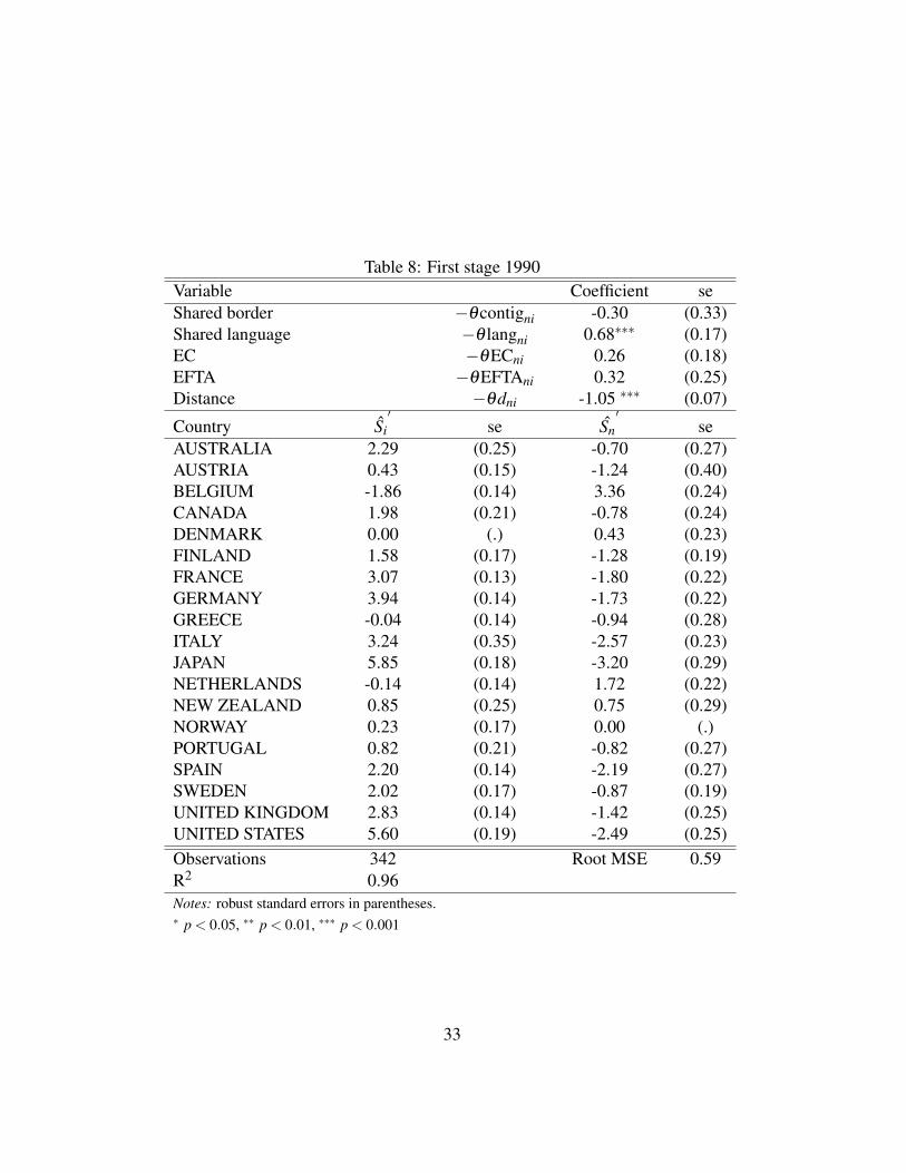
Table 8: First stage 1990
Variable Coefficient se
Shared border −θcontigni -0.30 (0.33)
Shared language −θ langni 0.68∗∗∗ (0.17)
EC −θECni 0.26 (0.18)
EFTA −θEFTAni 0.32 (0.25)
Distance −θdni -1.05 ∗∗∗ (0.07)
Country Si
′
se Sn
′
se
AUSTRALIA 2.29 (0.25) -0.70 (0.27)
AUSTRIA 0.43 (0.15) -1.24 (0.40)
BELGIUM -1.86 (0.14) 3.36 (0.24)
CANADA 1.98 (0.21) -0.78 (0.24)
DENMARK 0.00 (.) 0.43 (0.23)
FINLAND 1.58 (0.17) -1.28 (0.19)
FRANCE 3.07 (0.13) -1.80 (0.22)
GERMANY 3.94 (0.14) -1.73 (0.22)
GREECE -0.04 (0.14) -0.94 (0.28)
ITALY 3.24 (0.35) -2.57 (0.23)
JAPAN 5.85 (0.18) -3.20 (0.29)
NETHERLANDS -0.14 (0.14) 1.72 (0.22)
NEW ZEALAND 0.85 (0.25) 0.75 (0.29)
NORWAY 0.23 (0.17) 0.00 (.)
PORTUGAL 0.82 (0.21) -0.82 (0.27)
SPAIN 2.20 (0.14) -2.19 (0.27)
SWEDEN 2.02 (0.17) -0.87 (0.19)
UNITED KINGDOM 2.83 (0.14) -1.42 (0.25)
UNITED STATES 5.60 (0.19) -2.49 (0.25)
Observations 342 Root MSE 0.59
R2 0.96
Notes: robust standard errors in parentheses.∗ p < 0.05, ∗∗ p < 0.01, ∗∗∗ p < 0.001
33

Table 9: EK Competitiveness equation 1990 - Barro Lee/Cohen Soto
OLSbl 2SLSbl OLScs 2SLScs
lnWagesi -2.46∗∗ -3.40∗∗ -2.90∗∗ -4.03∗∗∗
(0.90) (1.34) ( 1.25) (1.29)
lnR&Di 1.22∗∗∗ 1.34∗∗∗ 1.19∗∗∗ 1.26∗∗∗
(0.15) (0.17) (0.13) (0.12)
1/Hi 6.71 7.10 -1.52 -7.44
(6.03) (7.59) (9.67) (10.28)
Constant 20.99 29.89∗∗ 26.09 37.52∗∗
(8.25) (12.00) (12.58) (12.74)
Observations 19 19 19 19
R2 0.78 0.76 0.79 0.77
Root MSE 1.02 1.06 1.00 1.04
Notes: robust standard errors in parentheses.∗ p < 0.05, ∗∗ p < 0.01, ∗∗∗ p < 0.001
The Si′ are then regressed on two proxies for technology (R&D expenditures and
average years of education) and wages corrected for worker quality. The second-
step regression is estimated twice, using different database for education: first
Barro and Lee (2010), then Cohen and Soto (2001). Since human capital is used
to correct both wages and labour force for worker quality, and it also appears as
a proxy for technology, a different database for education could lead to substan-
tial differences in the measure of the elasticity of trade.32 The structure of the
second stage specification is maintained identical to the original EK competitive-
ness equation: the inverse of the average years of schooling is used as a proxy for
human capital and the same EK instruments for wages have been used.
As can be observed from Table 9, the elasticity of trade obtained through 2SLS
ranges between 4.03 and 3.40 which I view as reassuring, since both estimates are
quite close to 3.60. Using a different database for education affects the estimation
of the elasticity of trade: the difference between the two 2SLS estimates is around
0.6. Finally, as in EK, the effect of education on country i competitiveness is not
statistically significant and only Cohen and Soto (2001) data give the expected
sign; as for R&D, both effects are similar in magnitude to the EK results.33
32This kind of experiment couldn’t be conducted for the whole sample of 27 countries for 1997,
since some of the data on education needed for the comparison are not available in Cohen-Soto
database.33The first stage results obtained using OLS with robust standard errors are almost identical to
34

A.3 One-step analysis
One-step specification. Head and Mayer (2013) identified in the literature 744
gravity based estimates of trade elasticity: many of these coefficients have been
estimated through a one-step procedure. In EK, for instance, two of the three
methodologies implemented to obtain an estimate of trade elasticity are one-step.
In what follows I estimate the same EK competitiveness equation for 1997 using
a one-step procedure. By plugging the determinants of Si′ into the EK bilateral
trade equation, I obtain the following one-step specification:
ln
[
X′ni
X′nn
]
= α0 +αR lnR&Di +αH lnHi −θ lnwi −Sn′−θ lndni
−θ langni −θcontigni −θRTAni +δ 1ni +δ 2
ni +ui
One-step and two-step methodologies are not equivalent. According to the liter-
ature, there may be substantial differences between one-step and two-step proce-
dures and generally the two-step technique is preferred. These differences involve
both (i) the magnitude as well as (ii) the standard errors of the coefficients.
(i) Baker and Fortin (2001) showed that the one-step methodology may lead
to biases in the coefficients if and only if the second-stage error term ui is not
orthogonal to the one-step regressors, namely geographic barriers, exporter
and importer fixed effects.34 Otherwise, all else being equal, the two proce-
dures should lead to similar estimates under the assumption that ui is truly
a random effect. In the equation above, the residual ui captures the impact
on country i’s competitiveness of variables other than wages and technology:
this effect in the one-step procedure should be incorporated in the error com-
ponent that affects trade one way. Thus, if the assumption of δni consisting
of two components both orthogonal to the first stage regressors is correct, ui
is also orthogonal to the one step regressors and the two procedures should
lead to similar estimates.
the ones obtained using WLS, which is just a special case of the more general estimating technique
GLS. As a consequence, both WLS and OLS fixed effects coefficients lead to identical measures
of θ . These results are available upon request.34The assumption I made for the competitiveness regression implies that ui is orthogonal to the
competitiveness determinants
35

Table 10: One-step estimations
OLS 2SLS OLS 2SLS
lnWagesi -3.99 -5.44 -0.00 -1.88
(2.73) (3.51) (0.16) ( 1.25)
lnR&Di 1.70∗∗∗ 1.83∗∗∗ 0.83∗∗∗ 1.67∗∗∗
(0.39) (0.41) (0.06) ( 0.29)
1/Hi 19.16 12.43 4.76 36.58
(14.98) (16.10) ( 4.90) (18.01)
Constant 20.88 34.00 0.82 2.16
(24.05) (33.07) (1.57) (8.23)
Observations 342 342 702 702
R2 0.83 0.83 0.86 0.82
Root MSE 1.85 1.87 0.78 2.03
Notes: standard errors clustered by exporter in parentheses.∗ p < 0.05, ∗∗ p < 0.01, ∗∗∗ p < 0.001
(ii) Since country characteristics are likely to be correlated within groups, the
estimated coefficients may show a much lower variance in the one-step proce-
dure when using heteroskedasticity consistent White robust standard errors.
Moulton (1986) argues that a possible cause for relatively lower standard er-
rors in the one-step procedure might be a source of downward bias due to the
correlation of individual error terms within groups; this may lead to serious
mistakes in statistical inference. This bias derives from using grouped data
in an individual level regression where groups are not allowed to be treated
as fixed parameters. To quantify the magnitude of this bias, Macpherson
and Hirsch (1995) found that the single step estimation produced coefficients
with standard errors ten times lower compared to the standard errors obtained
through the two-step procedure. To correct for the one-step Moulton bias, I
use standard errors clustered by country i. The number of clusters is crucial
to establish whether or not the standard cluster adjustment is reliable. Angrist
and Pischke (2009) argue that with few clusters there’s a tendency to under-
estimate the intraclass correlation in the Moulton problem. However, there’s
not a specific number of clusters considered as a threshold which separates a
reliable from an unreliable standard cluster adjustment. Angrist and Pischke
(2009) propose 42 which is way beyond the number of clusters of the whole
sample. 35
35The same authors seem a bit skeptical about this number, since the literature provides exam-
36
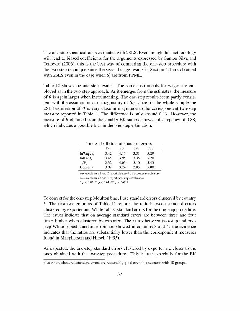
The one-step specification is estimated with 2SLS. Even though this methodology
will lead to biased coefficients for the arguments expressed by Santos Silva and
Tenreyro (2006), this is the best way of comparing the one-step procedure with
the two-step technique since the second stage results in Section 4.1 are obtained
with 2SLS even in the case when S′
i are from PPML.
Table 10 shows the one-step results. The same instruments for wages are em-
ployed as in the two-step approach. As it emerges from the estimates, the measure
of θ is again larger when instrumenting. The one-step results seem partly consis-
tent with the assumption of orthogonality of δni, since for the whole sample the
2SLS estimation of θ is very close in magnitude to the correspondent two-step
measure reported in Table 1. The difference is only around 0.13. However, the
measure of θ obtained from the smaller EK sample shows a discrepancy of 0.88,
which indicates a possible bias in the one-step estimation.
Table 11: Ratios of standard errors19c 27c 19c 27c
lnWagesi 3.42 4.17 3.31 5.29
lnR&Di 3.45 3.95 3.35 5.20
1/Hi 2.32 4.03 3.10 5.43
Constant 3.02 3.24 2.85 5.00
Notes:columns 1 and 2 report clustered by exporter se/robust se
Notes:columns 3 and 4 report two-step se/robust se∗ p < 0.05, ∗∗ p < 0.01, ∗∗∗ p < 0.001
To correct for the one-step Moulton bias, I use standard errors clustered by country
i. The first two columns of Table 11 reports the ratio between standard errors
clustered by exporter and White robust standard errors for the one-step procedure.
The ratios indicate that on average standard errors are between three and four
times higher when clustered by exporter. The ratios between two-step and one-
step White robust standard errors are showed in columns 3 and 4: the evidence
indicates that the ratios are substantially lower than the correspondent measures
found in Macpherson and Hirsch (1995).
As expected, the one-step standard errors clustered by exporter are closer to the
ones obtained with the two-step procedure. This is true especially for the EK
ples where clustered standard errors are reasonably good even in a scenario with 10 groups.
37

sample, as the first and third columns of Table 11 show very similar ratios for all
coefficients. The ratios reported in the second and fourth columns show a larger
discrepancy. This result is a bit surprising, since according to Angrist and Pischke
(2009) a higher number of clusters should imply a reduction in the Moulton bias
because of a lower intraclass correlation. My results seem to go in the opposite
direction.
38