WP/16/101

Estimating the Effects of the Trans-Pacific Partnership (TPP) on Latin America and the Caribbean (LAC)

by Diego A. Cerdeiro

2

© 2016 International Monetary Fund WP/16/101

Western Hemisphere Department

Estimating the Effects of the Trans-Pacific Partnership (TPP) on LAC

Prepared by Diego A. Cerdeiro1

Authorized for distribution by Valerie Cerra

May 2016

Abstract

In February 2016, twelve Pacific Rim countries signed the agreement on the Trans Pacific

Partnership (TPP), one of the largest and most comprehensive trade deals in history. While

there are several estimates of the likely effects of the TPP, there is no systematic study on the

effects on all Latin American countries. We present the results from applying a multi-sector

model with perfect competition presented by Costinot and Rodriguez-Clare (2014). The

exercise, based on input-output data for 189 countries and 26 sectors, shows that (i) Asian

TPP members are estimated to benefit most from the agreement, (ii) negative spillovers to

non-TPP LAC countries appear to be of a different order of magnitude than the gains of

members, and (iii) some non-TPP LAC countries may experience relatively large benefits

from joining the TPP. As a cautionary note, however, we point out that even a cursory cross-

study comparison shows that there is considerable uncertainty regarding the potential effects

of the TPP for both members and non-members.

JEL Classification Numbers: F11, F13, F14, F15, F17.

Keywords: TPP, Trans-pacific Partnership, LAC

Author’s E-Mail Address: dcerdeiro@imf.org

1 Strategy and Policy Review Department. This work was completed while I was at the Western Hemisphere

Department, as part of a broader project led by Valerie Cerra to assess trade integration in Latin America and

the Caribbean. I am very grateful to Valerie Cerra for continued support, and to Emine Boz, Nigel Chalk,

Metodij Hadzi-Vaskov, Christian Henn, Andras Komaromi, Natalija Novta, Marika Santoro and Alejandro

Werner for helpful comments and discussions. All remaining errors are my own.

IMF Working Papers describe research in progress by the author(s) and are published to

elicit comments and to encourage debate. The views expressed in IMF Working Papers are

those of the author(s) and do not necessarily represent the views of the IMF, its Executive Board,

or IMF management.

3

Contents Abstract ..................................................................................................................................... 2

Key findings ...................................................................................................................... 4

I. Introduction ........................................................................................................................... 4 II. Tariff and Non-Tariff Barriers ............................................................................................. 5 III. Estimating the Effects of the TPP: Framework and data .................................................... 8 IV. Estimates of the effects of the TPP on members and non-members ................................ 12 V. Comparison with other studies ........................................................................................... 17

VI. Expanding the TPP ........................................................................................................... 21 VII. Concluding remarks ........................................................................................................ 23

References ....................................................................................................................... 24

Appendix 1 ...................................................................................................................... 26 Appendix 2 ...................................................................................................................... 28

4

Key findings

Asian TPP members are estimated to benefit most from the agreement. Emerging Asian

economies appear to be among the members who would benefit most from the agreement.

This is likely a result of there being larger spillovers between each other, given that they have

proportionally stronger trade links with TPP partners. In LAC, Mexico is estimated to

experience gains of relatively similar size, while in comparison the estimated benefits for

Chile and Peru are more muted.

Negative spillovers to non-TPP LAC countries appear to be of a different order of

magnitude than the gains of members. As an indication, in our estimates the largest real

income gain within the TPP is more than 50 times larger than the absolute value of the

largest negative spillover within LAC. In general, economies that are more open and have

stronger existing trade with TPP members (especially with the U.S., such as many Central

America and Caribbean countries) tend to face larger negative spillovers. However, given the

TPP’s relatively liberal rules of origin, non-members participating in global value chains

integrated with TPP partners may actually be able to reap some benefits from the agreement.

Non-preferential reductions in non-tariff barriers may also produce positive spillovers to

LAC nonmembers.

Some non-TPP LAC countries may experience relatively large benefits from joining the

TPP. Out of nine non-TPP LAC countries considered, Colombia and Guatemala are

estimated to experience the largest gains from potential inclusion in the TPP: their estimated

gains are in fact larger than for some LAC countries in the TPP. Given current tariffs, many

LAC countries would experience a negative impact from full tariff liberalization vis-à-vis

TPP members; for those countries a potential inclusion in the TPP may require longer

negotiations.

I. INTRODUCTION

The TPP agreement, an ambitious trade deal, was signed in February 2016. In February

2016, Mexico, Chile and Peru, together with the United States, Canada and seven Asia-

Pacific countries (Australia, Brunei Darussalam, Japan, Malaysia, New Zealand, Singapore

and Vietnam) reached agreement on the Trans Pacific Partnership, one of the largest and

most comprehensive trade deals in history. Together, the 12 TPP partner countries represent

nearly 40 percent of world GDP, and the agreement covers frontier issues such as services,

investment, government procurement, SOEs, SMEs, intellectual property, labor,

environment, competition policy, etc that would imply a substantial fall in non-tariff barriers.

While there are several estimates of the likely effects of the TPP, there is no systematic

study on the effects on all Latin American countries. The aim of the present study to

provide a first set of estimates to start filling this gap. We present the results from applying

the multi-sector with perfect competition as presented by Costinot and Rodriguez-Clare

(2014). The model is simple enough to be able to provide estimates for a large number of

countries, some of which are relatively small. The exercise is based on input-output data for

189 countries and 26 sectors.

5

The rest of the paper is organized as follows. In Section 2 we describe the tariffs and non-

tariff barriers of TPP members. Section 3 briefly discussed the model and presents the input-

output data to be used. The estimates of the effects of the TPP on members and non-members

are presented in Section 4. Section 5 compares and discusses the results in the light of those

of other studies. Section 6 considers the potential effects for certain non-TPP LAC countries

of being included in an expanded TPP. Section 7 concludes.

II. TARIFF AND NON-TARIFF BARRIERS

Tariff data between TPP countries were obtained from the Market Access Map

(MAcMap), which provides an overall ad-valorem equivalent of applied protection.2 For

eight countries (Australia, Brunei Darussalam, Japan, New Zealand, Peru, Singapore, U.S.,

and Vietnam) the data correspond to 2014. For the remaining four TPP members, latest

available data are used (2013 for Canada, 2009 for Mexico, 2008 for Chile, and 2007 for

Malaysia). There are 683.6 thousand HS 6-digit lines in the dataset. Tariffs dating from 2012

and later are originally classified in HS 2012, and were converted into HS 2007 using the UN

conversion tables.3 Once all tariff data are in HS 2007 format, they were matched with trade

data from Comtrade (HS 2007 classification) for the year 2012 (the same year of the world

input-output data used). The merged data were then converted into SITC Rev. 3 classification

using UN conversion tables, to finally convert it to the 26-sector classification used by Eora.

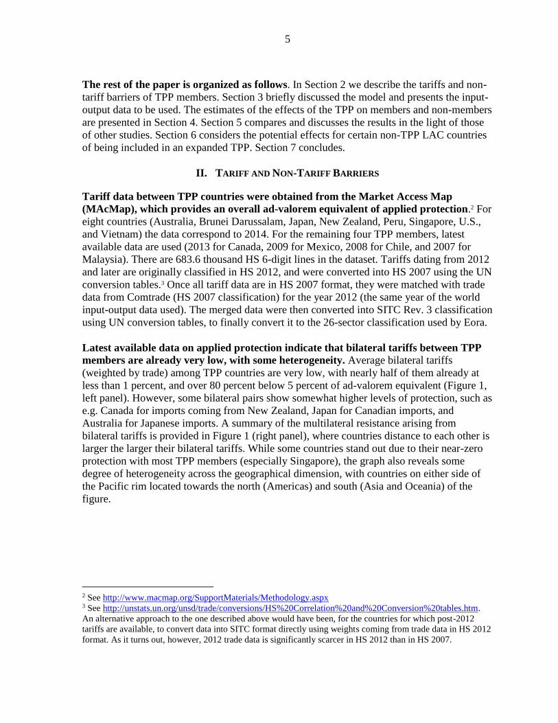
Latest available data on applied protection indicate that bilateral tariffs between TPP

members are already very low, with some heterogeneity. Average bilateral tariffs

(weighted by trade) among TPP countries are very low, with nearly half of them already at

less than 1 percent, and over 80 percent below 5 percent of ad-valorem equivalent (Figure 1,

left panel). However, some bilateral pairs show somewhat higher levels of protection, such as

e.g. Canada for imports coming from New Zealand, Japan for Canadian imports, and

Australia for Japanese imports. A summary of the multilateral resistance arising from

bilateral tariffs is provided in Figure 1 (right panel), where countries distance to each other is

larger the larger their bilateral tariffs. While some countries stand out due to their near-zero

protection with most TPP members (especially Singapore), the graph also reveals some

degree of heterogeneity across the geographical dimension, with countries on either side of

the Pacific rim located towards the north (Americas) and south (Asia and Oceania) of the

figure.

2 See http://www.macmap.org/SupportMaterials/Methodology.aspx 3 See http://unstats.un.org/unsd/trade/conversions/HS%20Correlation%20and%20Conversion%20tables.htm.

An alternative approach to the one described above would have been, for the countries for which post-2012

tariffs are available, to convert data into SITC format directly using weights coming from trade data in HS 2012

format. As it turns out, however, 2012 trade data is significantly scarcer in HS 2012 than in HS 2007.

6

Figure 1. Average bilateral tariffs

Histogram (left) and spring graph (right) 1/

1/ Each arrow in the spring graph acts as a spring, tying the source (exporter) and destination (importer) nodes

closer together. Spring strengths and widths are proportional to the logarithm of the inverse of bilateral tariffs.

We thank F. Diebold and K. Yilmaz for sharing their implementation of the ForceAtlas2 algorithm in Gephi.

Source: Authors’ calculations based on MAcMap and Comtrade.

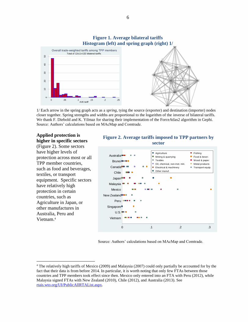
Applied protection is

higher in specific sectors

(Figure 2). Some sectors

have higher levels of

protection across most or all

TPP member countries,

such as food and beverages,

textiles, or transport

equipment. Specific sectors

have relatively high

protection in certain

countries, such as

Agriculture in Japan, or

other manufactures in

Australia, Peru and

Vietnam.4

4 The relatively high tariffs of Mexico (2009) and Malaysia (2007) could only partially be accounted for by the

fact that their data is from before 2014. In particular, it is worth noting that only few FTAs between those

countries and TPP members took effect since then. Mexico only entered into an FTA with Peru (2012), while

Malaysia signed FTAs with New Zealand (2010), Chile (2012), and Australia (2013). See

rtais.wto.org/UI/PublicAllRTAList.aspx.

01

02

03

04

05

0

De

nsity

0 .05 .1 .15 .2 .25AVE tariff

Total of 12x11=132 bilateral tariffs

Overall trade-weighted tariffs among TPP members

Figure 2. Average tariffs imposed to TPP partners by

sector

Source: Authors’ calculations based on MAcMap and Comtrade.

0 .1 .2 .3

Vietnam

U.S.

Singapore

Peru

New Zealand

Mexico

Malaysia

Japan

Chile

Canada

Brunei

AustraliaAgriculture Fishing

Mining & quarrying Food & bever.

Textiles Wood & paper

Oil, chemical, non-met. min. Metal products

Electrical & machinery Transport equip.

Other manuf.

7

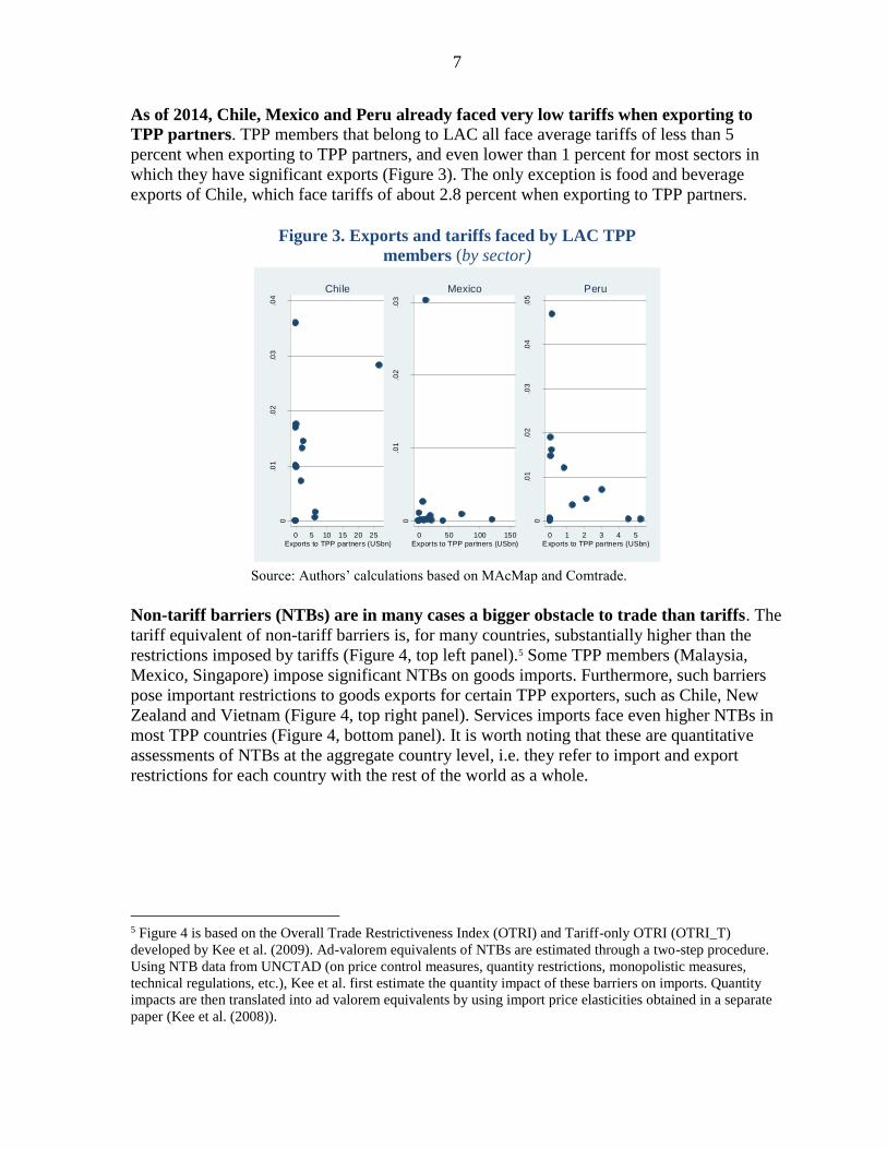
As of 2014, Chile, Mexico and Peru already faced very low tariffs when exporting to

TPP partners. TPP members that belong to LAC all face average tariffs of less than 5

percent when exporting to TPP partners, and even lower than 1 percent for most sectors in

which they have significant exports (Figure 3). The only exception is food and beverage

exports of Chile, which face tariffs of about 2.8 percent when exporting to TPP partners.

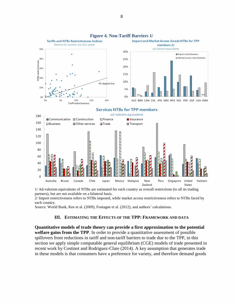
Non-tariff barriers (NTBs) are in many cases a bigger obstacle to trade than tariffs. The

tariff equivalent of non-tariff barriers is, for many countries, substantially higher than the

restrictions imposed by tariffs (Figure 4, top left panel).5 Some TPP members (Malaysia,

Mexico, Singapore) impose significant NTBs on goods imports. Furthermore, such barriers

pose important restrictions to goods exports for certain TPP exporters, such as Chile, New

Zealand and Vietnam (Figure 4, top right panel). Services imports face even higher NTBs in

most TPP countries (Figure 4, bottom panel). It is worth noting that these are quantitative

assessments of NTBs at the aggregate country level, i.e. they refer to import and export

restrictions for each country with the rest of the world as a whole.

5 Figure 4 is based on the Overall Trade Restrictiveness Index (OTRI) and Tariff-only OTRI (OTRI_T)

developed by Kee et al. (2009). Ad-valorem equivalents of NTBs are estimated through a two-step procedure.

Using NTB data from UNCTAD (on price control measures, quantity restrictions, monopolistic measures,

technical regulations, etc.), Kee et al. first estimate the quantity impact of these barriers on imports. Quantity

impacts are then translated into ad valorem equivalents by using import price elasticities obtained in a separate

paper (Kee et al. (2008)).

Figure 3. Exports and tariffs faced by LAC TPP

members (by sector)

Source: Authors’ calculations based on MAcMap and Comtrade.

0

.01

.02

.03

.04

AV

E t

ariff

0 5 10 15 20 25

Exports to TPP partners (USbn)

Chile

0

.01

.02

.03

0 50 100 150

Exports to TPP partners (USbn)

Mexico

0

.01

.02

.03

.04

.05

0 1 2 3 4 5

Exports to TPP partners (USbn)

Peru

8

Figure 4. Non-Tariff Barriers 1/

1/ Ad-valorem equivalents of NTBs are estimated for each country as overall restrictions (to all its trading

partners), but are not available on a bilateral basis.

2/ Import restrictiveness refers to NTBs imposed, while market access restrictiveness refers to NTBs faced by

each country.

Source: World Bank, Kee et al. (2009), Fontagne et al. (2012), and authors’ calculations.

III. ESTIMATING THE EFFECTS OF THE TPP: FRAMEWORK AND DATA

Quantitative models of trade theory can provide a first approximation to the potential

welfare gains from the TPP. In order to provide a quantitative assessment of possible

spillovers from reductions in tariff and non-tariff barriers to trade due to the TPP, in this

section we apply simple computable general equilibrium (CGE) models of trade presented in

recent work by Costinot and Rodriguez-Clare (2014). A key assumption that generates trade

in these models is that consumers have a preference for variety, and therefore demand goods

0%

10%

20%

30%

40%

50%

0% 5% 10% 15% 20%

Tariffs and NTBs Restrictiveness IndicesBased on 63 countries, July 2012 update

Tariff restrictiveness

NTB

s re

stri

ctiv

en

ess

45-degree line

0%

5%

10%

15%

20%

25%

30%

AUS BRN CAN CHL JPN MEX MYS NZL PER SGP USA VNM

Import and Market Access Goods NTBs for TPP

members 2/ad valorem equivalents

Import restrictiveness

Market access restrictiveness

N/A N/A

0

20

40

60

80

100

120

140

160

180

Australia Brunei Canada Chile Japan Mexico Malaysia New

Zealand

Peru Singapore United

States

Vietnam

Services NTBs for TPP membersad-valorem equivalents

Communication Construction Finance Insurance

Business Other services Trade Transport

9

Sector Elasticity

Agriculture 8.11

Fishing 8.11

Mining & quarrying 15.72

Food & beverages 2.55

Textiles & wearing apparel 5.56

Wood & paper 10.83

Petroleum, chemica & non-metallic mineral products 19.53*

Metal products 4.50

Electrical & machinery 10.60

Transport equipment 0.69**

Other 5.00

* Simple average of Petroleum (51.08), Chemicals (4.75), and Non-metallic

mineral products (2.76).

** Simple average of Auto (1.01), and Other transport (0.37).

Source: Caliendo and Parro (2015)

Table 1. Elasticities

from different sources.6 Utility is assumed to be linear in real consumption, and the different

varieties of goods in the consumption basket are aggregated using a constant elasticity of

substitution (CES) function. Since there is no investment or government consumption in the

model, and trade balances are zero,7 it is natural to interpret changes in welfare/real

consumption as changes in real income. It is also worth noting that, as a result of these

assumptions, access to more varieties of a good can increase real income by reducing the

price of one unit of (CES-aggregated) consumption (see e.g. Broda and Weinstein (2006)).

The model is chosen with the aim of providing estimates for a large number of

countries. When choosing which model to apply, there is a tradeoff between the model’s

complexity and the granularity of the data that can be used as inputs. We present the results

from applying the multi-sector with perfect competition as presented by Costinot and

Rodriguez-Clare (2014).8 In Section 5, when comparing our results with those found

elsewhere in the literature, we discuss some channels that our model of choice does not

capture.

Thanks to recent advances in trade theory modeling methods, the data requirements

for the quantitative exercise are relatively few. Models of international trade typically

feature a series of structural parameters that are very hard to estimate in practice. A case in

point are bilateral non-tariff barriers (see the discussion of the previous section), which in

trade theory models would add up to

“iceberg costs” of trading between pairs

of countries. A method popularized by

Dekle, Eaton and Kortum (2007)

circumvents this problem by simply

formulating the equilibrium in changes

rather than in levels. As pointed out by

Ossa (forthcoming), the method

“[e]ssentially […] imposes a restriction

on the set of unknown parameters […]

such that the predicted [initial trade flows]

perfectly match the observed [trade

flows].” Thus, instead of requiring the

level of bilateral NTBs before and after

the specific trade agreement under study,

this method only requires the percent change in these barriers. As will be discussed next,

constructing an assumption on how a trade agreement reduces bilateral barriers to trade is not

exempt from

6 This idea, first modeled by Armington (1969), was popularized by Dixit and Stiglitz (1977) and first applied to

trade by Krugman (1979). In new trade theory models with imperfect competition, economies of scale provide

an additional incentive to trade. 7 Following what is becoming a standard practice (Costinot and Rodriguez-Clare (2014), Ossa (2015)), the raw

data is first purged from trade imbalances by performing the exercise proposed by Dekle et al. (2007). 8 Appendix I also shows the results when applying the simpler single-sector Armington model. No algorithm

was found that could solve the other models presented in Costinot and Rodriguez-Clare (2014) for the large

dataset used in this study. Appendix II describes some main features of the model in more detail.

10

difficulties, but the method nonetheless reduces dramatically the number of parameters the

model requires.9

The exercise is based on input-output data for 189 countries and 26 sectors. Data on

international trade and domestic absorption for 189 countries and 26 sectors for the year 2012

is available from the Eora Multi-Region Input-Output (MRIO) table (Lenzen et al. (2012,

2013)). The tariff data from MAcMap is converted into the Eora sector classification using

2012 HS 6-digit bilateral

trade data from Comtrade as

weights. In the model with

multiple sectors, utility

functions consist of two

layers. At the higher layer, the

elasticity of substitution

across different sectors is

assumed to be equal to one.

The lower level aggregates

different varieties of goods

within the same sector.

Estimating elasticities of

substitution for different

varieties is beyond the scope

of this study. Following the

approach of Costinot and

Rodriguez-Clare (2014), we

instead match the elasticity

estimates of Caliendo and

Parro (2015) to the sectors in

our dataset (Table 1).

NTBs are assumed to drop to the levels of those TPP members with less restrictive

trade regimes. The high level of NTBs of some of the TPP members is expected to be

reduced as a result of the agreement.10 As can be seen in Figure 4 (top right panel), Chile has

the lowest level of NTBs applied to goods imports (2.5 percent). In the exercise below, we

9 For example, in a dataset with 189 countries, solving the Armington (i.e. single-sector) model in levels would

require the level of NTBs for 189x188=35,532 directed bilateral pairs, in addition to the post-agreement NTBs

between the 12x11=132 directed bilateral pairs between TPP members and the elasticity of substitution across

goods from different countries. By only requiring the change in NTBs for the 132 directed bilateral pairs in the

TPP (alongside the elasticity of substitution), the “exact-hat algebra” technique popularized by Dekle et al.

(2007) effectively cuts the cardinality of the parameter set by 35,532. 10 With the exception of chapters related to tariffs (2-4, 6), labor (19), and environment (20), most chapters in

the TPP agreement are expected to lead in some way to a reduction in NTBs among members. Among the ones

most closely related are chapters 5 (on custom administration and trade facilitation),7 (sanitary and

phitosanitary measures), 8 (technical barriers to trade), 9 (investment), 10 (cross border trade in services), 13

(telecommunications), 14 (electronic commerce), 15 (government procurement), 16 (competition), and 22

(competitiveness and business facilitation).

Figure 5. TPP members’ goods and services trade by

selected groups of trading partners

as percent of GDP

Source: Eora MRIO and authors’ calculations.

AUS BRN CAN CHL JPN MYS MEX NZL PER SGP USA VNM0

50

100

150

200

250

TPP LAC

USA & CAN

TPP Asia

Other LAC

Other

11

assume that NTBs for trade in goods

between TPP members drop to this level.11

Ad-valorem equivalents of NTBs on services

imports are available at the sector level from

Fontagne et al (2012) (see Figure 4, bottom

panel).12 We assume that, with the entry into

force of the TPP, NTBs for every TPP

country are reduced to the level of the U.S.

(unless for that sector NTBs are already

lower than those in the U.S.). We then apply

the average decrease in NTBs to all the

services sectors present in the Eora dataset.

Figure 6 summarizes the assumed drop in

NTBs in goods and services for every TPP

member.13

11 No estimates for Brunei and Vietnam are available in the 2012 World Bank update of trade restrictiveness

indices. For Brunei, we took the earlier estimate by Kee et al. (2009). For Vietnam, we imputed the simple

average of the indices for Malaysia and Singapore. 12 Given the lack of estimates for Brunei and Vietnam for services NTBs, we imputed the simple average of the

indices for Malaysia and Singapore. 13 Note that we are assuming that the reduction in NTBs is purely preferential. This is a deliberate choice that

stacks the deck against non-members, so as to obtain upper bounds on the potential negative effects of the

agreement. As highlighted in Henn et al. (2016), some studies assume a certain extent of non-discriminatory

reduction in NTBs, although there is no solid empirical evidence of their size.

Figure 6. Assumed Reduction in NTBs 1/

in percent

1/ If τ and τ’ denote the ad-valorem NTBs before and

after the agreement, then the chart shows, for each

member, ((1+ τ’)/(1+ τ)-1)*100.

Source: Authors’ calculations.

-20 -15 -10 -5 0

Australia

Brunei

Canada

Chile

Japan

Malaysia

Mexico

New Zealand

Peru

Singapore

United States

Vietnam

Services

Goods

12

IV. ESTIMATES OF THE EFFECTS OF THE TPP ON MEMBERS AND NON-MEMBERS

The estimated effects of further tariff liberalization on TPP members are relatively

small. Table 3 shows the effect of elimination of bilateral tariffs between TPP.14 Each row

shows the welfare (or real consumption/real income) effect, in percent change, on that row’s

country of the tariff reductions indicated by each column. Columns 2 through 13 correspond

to elimination of all tariffs that the TPP member of that column faces when exporting to TPP

partners, while the last column (column 14) corresponds to elimination of all tariffs between

TPP members. For example, the first column for Australia shows the welfare effects on each

TPP member if TPP members eliminated all existing tariffs on Australian exports;

Australia’s welfare would increase by 0.09 percent, whereas Malaysia’s would fall by 0.02

percent. In general, inspection of the diagonal elements of columns 2-13 show that, while all

countries would gain from lower tariffs when exporting to TPP partners’ markets, the gains

are generally small and somewhat heterogeneous. The gains from unilateral better access

range from 0.23 percent for New Zealand, to 0.01 percent for Brunei and Mexico.

Interestingly, New Zealand’s gains from lower tariffs do not generate significant negative

effects on the countries reducing their tariffs, with Malaysia’s welfare dropping by merely

0.01 percent.15 Of the three LAC countries, Chile stands most to gain (0.11 percent), which is

consistent with the observation of the previous section that Chile faces large tariffs in food

and beverages exports to TPP partners. Gains from elimination of all tariffs between TPP

members are also small, and in some cases (Peru, and especially Vietnam) negative.

Tariff reductions among TPP members are estimated to have negligible effects on LAC

non-TPP members. Table 4 shows the effect of tariff reductions among TPP members on

14 While the TPP agreement incorporates exceptions and different phase-out transitions, the exercise presented

in Table 3 shows the maximum scope for welfare gains/losses from tariff reductions. It has been reported that

99 percent of nonzero tariff lines will eventually fall to zero under the TPP (Petri and Plumer (2016)). 15 In some instances, off-diagonal elements in Table 3 are positive. For example, Vietnam benefits from the

elimination of all tariffs on Australian exports to TPP partners. This is a result of Malaysia’s goods and services

becoming cheaper in world markets.

Australia Brunei Canada Chile Japan Malaysia MexicoNew

ZealandPeru Singapore USA Vietnam

Australia 0.09 0.00 0.00 0.00 0.00 0.00 0.00 0.00 0.00 0.00 -0.01 0.00 0.06

Brunei 0.00 0.01 0.00 0.00 0.01 0.00 0.00 0.00 0.00 -0.01 0.00 0.00 0.01

Canada 0.00 0.00 0.06 0.00 0.00 0.00 0.00 0.00 0.00 0.00 0.00 0.00 0.03

Chile 0.00 0.00 0.00 0.11 0.00 0.00 0.00 0.00 0.00 0.00 -0.01 0.00 0.07

Japan 0.01 0.00 0.00 0.00 0.02 0.00 0.00 0.00 0.00 0.00 0.00 0.00 0.04

Malaysia -0.02 0.00 0.00 0.00 -0.05 0.05 0.00 -0.01 0.00 -0.02 0.09 0.00 0.07

Mexico 0.00 0.00 -0.02 0.02 -0.02 0.00 0.01 0.00 0.00 0.00 -0.02 0.00 0.01

New Zealand 0.00 0.00 0.00 0.00 0.01 0.00 0.00 0.23 0.00 0.00 -0.03 0.00 0.20

Peru 0.00 0.00 0.00 0.00 0.00 0.00 0.00 0.00 0.03 0.00 -0.02 0.00 -0.01

Singapore 0.00 0.00 0.00 0.00 -0.01 0.00 0.00 0.00 0.00 0.05 -0.01 0.00 0.02

USA 0.00 0.00 0.00 0.00 0.00 0.00 0.00 0.00 0.00 0.00 0.03 0.00 0.03

Vietnam 0.02 0.00 0.01 0.00 -0.04 -0.01 0.00 0.00 0.00 -0.16 0.00 0.08 -0.11

Elimination of tariffs faced by column country's exports to TPP partners Full

liberalizati

on

Table 3. Welfare/real income effect of tariff liberalization

Notes: The results are based on a multi-sector model of trade with perfect competition as presented by Costinot and Rodriguez-Clare (2014). Each row shows the welfare

effect (in percent change) on that row's country of the tariff reductions indicated by each column. Columns 2 to 13 correspond to elimination of all tariffs that the TPP

member of that column faces when exporting to TPP partners. Column 14 corresponds to elimination of all tariffs between TPP members.

13

LAC countries that are not in the TPP. All in all, the results show that further tariff

reductions among TPP members would generate minor spillovers in the region.

Reductions in NTBs would have heterogeneous effects on TPP members, with

developing countries with stronger existing trade links within the TPP experiencing

larger gains. Table 5 shows the welfare effects of reductions in NTBs for TPP members.

Columns (a)-(c) display the welfare effect from reduction of NTBs in goods sectors, services

sectors, and both. Mainly Malaysia, but also Singapore, Vietnam and Mexico, would benefit

significantly from the reduction of NTBs. The countries that benefit most, do so mainly

through the reduction of NTBs in goods, with the lower services NTBs having comparatively

smaller effects. The effect of reducing obstacles to services trade has higher effects than the

removal of barriers to trade in goods only for Australia and Chile. Within LAC, Peru and

Chile benefit significantly less from NTBs reductions, partly as a result of having weaker

trade links with TPP members (especially when compared to the U.S.-Mexico trade), but also

because ex-ante it already has one of the least restrictive trade regimes. The welfare effects

are also related to the countries’ size, as Japan and the U.S. show the smallest welfare gains

among all members. For these two countries (as well as for New Zealand and Chile), gains

from full tariff liberalization would represent larger shares of the total potential welfare gains

(cf. column (c) with the last column in Table 5).

Australia Brunei Canada Chile Japan Malaysia MexicoNew

ZealandPeru Singapore USA Vietnam

Antigua 0.00 0.00 0.00 0.00 0.00 0.00 0.00 0.00 0.00 0.00 -0.02 0.00 -0.02

Argentina 0.01 0.01 0.01 0.02 0.01 0.01 0.01 0.01 0.01 0.01 0.00 0.01 0.01

Bahamas 0.00 0.00 0.00 0.00 0.00 0.00 0.00 0.00 0.00 0.00 -0.03 0.00 -0.03

Barbados 0.00 0.00 0.00 0.00 0.00 0.00 0.00 0.00 0.00 0.00 -0.01 0.00 -0.01

Belize 0.00 0.00 0.00 0.00 0.00 0.00 0.00 0.00 0.00 0.00 -0.01 0.00 -0.01

Bolivia 0.02 0.02 0.02 0.00 0.02 0.02 0.02 0.02 0.02 0.02 0.01 0.02 0.00

Brazil 0.00 0.00 0.00 0.00 0.00 0.00 0.00 0.00 0.00 0.00 0.00 0.00 0.00

Cayman Islands 0.00 0.00 0.00 0.00 0.00 0.00 0.00 0.00 0.00 0.00 -0.01 0.00 0.00

Colombia 0.01 0.01 0.01 0.00 0.01 0.01 0.01 0.01 0.01 0.01 0.00 0.01 0.00

Costa Rica 0.00 0.00 0.00 0.00 0.00 0.00 0.00 0.00 0.00 0.00 -0.01 0.00 -0.01

Cuba 0.00 0.00 0.00 0.00 0.00 0.00 0.00 0.00 0.00 0.00 0.00 0.00 0.00

Dominican Republic 0.00 0.00 0.00 0.00 0.00 0.00 0.00 0.00 0.00 0.00 0.00 0.00 0.00

Ecuador 0.00 0.00 0.00 0.00 0.00 0.00 0.00 0.00 0.00 0.00 0.00 0.00 0.00

El Salvador 0.00 0.00 0.00 0.00 0.00 0.00 0.00 0.00 0.00 0.00 -0.01 0.00 -0.01

Guatemala 0.00 0.00 0.00 0.00 0.00 0.00 0.00 0.00 0.00 0.00 -0.01 0.00 -0.02

Guyana 0.00 0.00 0.00 0.00 0.00 0.00 0.00 0.00 0.00 0.00 0.00 0.00 0.00

Haiti 0.00 0.00 0.00 0.00 0.00 0.00 0.00 0.00 0.00 0.00 0.00 0.00 0.00

Honduras 0.00 0.00 0.00 0.00 0.00 0.00 0.00 0.00 0.00 0.00 -0.01 0.00 -0.01

Jamaica 0.00 0.00 0.00 0.00 0.00 0.00 0.00 0.00 0.00 0.00 0.00 0.00 0.00

Nicaragua 0.00 0.00 0.00 0.00 0.00 0.00 0.00 0.00 0.00 0.00 -0.01 0.00 -0.01

Panama 0.00 0.00 0.00 0.00 0.00 0.00 0.00 0.00 0.00 0.00 -0.01 0.00 -0.01

Paraguay 0.00 0.00 0.00 0.00 0.00 0.00 0.00 0.00 0.00 0.00 0.00 0.00 0.00

Suriname 0.00 0.00 0.00 0.00 0.00 0.00 0.00 0.00 0.00 0.00 0.00 0.00 0.00

Trinidad and Tobago 0.00 0.00 0.00 0.00 0.00 0.00 0.00 0.00 0.00 0.00 0.01 0.00 0.00

Uruguay 0.00 0.00 0.00 0.00 0.00 0.00 0.00 0.00 0.00 0.00 -0.01 0.00 -0.01

Venezuela 0.00 0.00 0.00 0.00 0.00 0.00 0.00 0.00 0.00 0.00 0.00 0.00 0.00

Table 4. Welfare/real income spillovers in LAC of tariff liberalizationElimination of tariffs faced by column country's exports to TPP partners Full

liberalizati

on

Notes: The results are based on a multi-sector model of trade with perfect competition as presented by Costinot and Rodriguez-Clare (2014). Each row shows the welfare effect (in

percent change) on that row's country of the tariff reductions indicated by each column. Columns 2 to 13 correspond to elimination of all tariffs that the TPP member of that column

faces when exporting to TPP partners. Column 14 corresponds to elimination of all tariffs between TPP members.

14

Spillovers from reductions in NTBs appear stronger in Asia. The left panel in Figure 7

decomposes the total benefits in NTBs reduction of Table 5 (column (c)) into three

components: the benefits that a TPP member gets for reducing its own NTBs (“Internal

effect”), the spillovers from reductions in NTBs of TPP partners, and a residual accounting

for general-equilibrium effects (“Synergies”).16 Among the biggest beneficiaries of TPP,

Malaysia, Singapore, and Vietnam receive relatively large spillovers, whereas Mexico’s

gains are mainly related to its own reduction in barriers. The panel on the right of Figure 6

further breaks down the spillovers by origin. Malaysia and Singapore benefit substantially

from each other’s reduction in trade barriers, while Vietnam’s spillovers are mainly related

due to Singapore and Japan. The reduction in NTBs by the U.S. benefits Canada and Mexico,

but it is not large enough to generate relatively large effects.

16 The decomposition is obtained by running the model once for each TPP partner, where each simulation

corresponds to a single TPP member unilaterally reducing its barriers with the rest of the membership.

Goods

(a)

Services

(b)

Goods+Services

(c)

W/full tariff

liberalization

Australia 0.11 0.25 0.37 0.43

Brunei 0.24 0.07 0.31 0.34

Canada 0.15 0.09 0.24 0.27

Chile 0.09 0.15 0.24 0.33

Japan 0.06 0.06 0.12 0.17

Malaysia 3.10 0.17 3.27 3.58

Mexico 1.20 0.29 1.47 1.38

New Zealand 0.36 0.17 0.53 0.80

Peru 0.13 0.11 0.24 0.23

Singapore 1.71 0.11 1.82 1.70

USA 0.07 0.02 0.08 0.12

Vietnam 1.17 0.35 1.52 1.23

Reduction of NTBs in:

Table 5. Welfare/real income effect of NTBs and tariffs reduction

Notes: The results are based on a multi-sector model of trade with perfect competition as presented by

Costinot and Rodriguez-Clare (2014). Each row shows the welfare effect (in percent change) on that

row's country of the NTBs reduction described in the text.

Figure 7. Internal Effects, Spillovers, and Synergies

Decomposition

Spillovers

Source: Authors’ calculations.

AUSBRNCAN CHL JPNMYSMEXNZL PERSGPUSAVNM0

0.5

1

1.5

2

2.5

3

3.5

Internal

Spillovers

Synergies

AUS BRN CAN CHL JPN MYS MEX NZL PER SGP USA VNM-0.1

0

0.1

0.2

0.3

0.4

0.5

0.6

0.7

Spill

overs

AUS

BRN

CAN

CHL

JPN

MYS

MEX

NZL

PER

SGP

USA

VNM

15

Openness is estimated to increase for all members as a result of the TPP, with limited

trade diversion in general and no significant diversion away from LAC non-TPP

members.17 Total trade in goods and services as percent of GDP is estimated to increase by

between 2 percent of GDP for the U.S. to nearly 30 percent of GDP for Malaysia (Figure 8,

left panel). Mexico’s trade to GDP ratio is estimated to increase by about 18 p.p., mainly due

to deeper integration with the U.S. and Canada. Even for Chile and Peru, which are estimated

to gain relatively less in terms of real income, are estimated to increase their openness by

about 4 p.p. Trade diversion appears limited, mostly circumscribed to Singapore, Malaysia

and Vietnam. Trade diversion away from LAC is almost negligible, when measured as a

percent of the GDP of TPP members. When measured as percent of LAC countries GDP,

trade diversion is in the worst cases of less than 0.7 percent of GDP (Figure 10). Of course,

LAC non-TPP members do lose out share in trade of TPP members (especially LAC TPP

members and the U.S.; see Figure 8, right panel).

Figure 8. Changes in trade patterns

As percent of GDP

Changes in total trade

Changes in shares of total trade

Source: Authors’ calculations.

17 Note that the term “trade diversion” is being used loosely here. Reductions in NTBs among TPP members

reduce the cost of supplying goods between them; to the extent that members re-source towards more efficient

suppliers this is not sensu stricto trade diversion.

AUS BRN CAN CHL JPN MYS MEX NZL PER SGP USA VNM-20

-10

0

10

20

30

40

TPP LAC

USA & CAN

TPP Asia

Other LAC

Other

AUS BRN CAN CHL JPN MYS MEX NZL PER SGP USA VNM-25

-20

-15

-10

-5

0

5

10

15

20

25

TPP LAC

USA & CAN

TPP Asia

Other LAC

Other

16

Smaller and more open LAC economies and those with stronger links to TPP members

may face negative effects, but spillovers are of a different order of magnitude. Figure 9

shows the spillover effects on LAC countries of the reduction in NTBs within the TPP. The

negative effects are typically

much smaller than those

experienced within the TPP.

For example, the largest gain

within the TPP from reducing

NTBs in goods and services

(9.85 for Malaysia) is more

than 50 times larger than the

absolute value of the largest

spillover within LAC (-0.05

for Bahamas). In general,

economies that are more open

and have stronger existing

trade with TPP members

(especially with the U.S.,

such as many Central

America and Caribbean

countries) tend to face larger

negative spillovers.

Figure 10. Changes in LAC trade patterns In percent of each country’s GDP

Source: Authors’ calculations.

ATG ARG BHS BRB BLZ BOL BRA CYM COL CRI CUBDOM ECU SLV GTM GUY HTI HND JAM NIC PAN PRY SUR TTO URY VEN-0.8

-0.6

-0.4

-0.2

0

0.2

0.4

0.6

TPP LAC

USA & CAN

TPP Asia

Other LAC

Other

Figure 9. Spillovers to LAC Percent change in real income/welfare

Full tariff liberalization + NTBs reduction within TPP

Source: Authors’ calculations.

-0.09

-0.08

-0.07

-0.06

-0.05

-0.04

-0.03

-0.02

-0.01

0.00

0.01

Baham

as

Antig

ua

Beliz

e

Co

sta R

ica

Guate

mala

Panam

a

Barb

ad

os

El S

alv

ad

or

Bo

livia

Caym

an Isl

and

s

Ho

nd

ura

s

Nic

ara

gua

Ecu

ad

or

Suri

nam

e

Haiti

Jam

aic

a

Co

lom

bia

Uru

guay

Guya

na

Tri

nid

ad

and

To

bag

o

Cub

a

Bra

zil

Para

guay

Arg

entina

Do

min

ican R

ep

ub

lic

Venezu

ela

17

V. COMPARISON WITH OTHER STUDIES

The results of previous studies focusing on TPP members provide a benchmark for

comparison. Petri, Plummer and Zhai (2011) is the most widely cited paper providing CGE

estimates of the effects of the TPP (see Henn et al. (2016) for a comprehensive survey of TPP

studies). The study’s focus is on the effect on members, dividing the world into 24 regions.

While agriculture, mining and government services are assumed to operate under perfect

competition (as do all sectors in the model used in the present study), manufacturing and

private services are produced under monopolistic competition as in Melitz (2003). Thus,

reductions in tariffs and non-tariff barriers affect welfare not just through the intensive

margin (more trade of the same varieties), but also through the extensive margin (trade of

new products). Another important study on the TPP is due to Aichele and Felbermayr (2015),

who rely on an extended version of the model by Caliendo and Parro (2015). While the

model assumes perfect competition, it differs from the model used above in two dimensions.

First, capital is a second factor of production (a feature also present in Petri and Plummer

(2011)). Lower tariffs and non-tariff measures can thus lead to gains through higher

specialization. Second, by incorporating the production of intermediate goods, it may capture

gains for non-members that participate in value chains with members.18

Vietnam and Malaysia are consistently found to be among the biggest winners. Table 6

shows how different studies have ranked TPP members according to their gains from the

agreement (we include the updated results of Petri, Plummer and Zhai (2011) performed by

Petri and Plummer (2016)). Malaysia and Vietnam are consistently ranked among the

members who would benefit most from the agreement.

Results differ in terms of the average gains and some countries’ relative standing. Some

differences in the results across studies are apparent. Perhaps most remarkable are (i) the fact

that in the present study gains are smaller on average, and (ii) that we find relatively higher

gains for Mexico (Mexico is in fact a loser in Aichele and Felbermayr (2015), due to the loss

of preferential access to the U.S.).

Firm entry and the presence of global value chains are likely to amplify gains from the

TPP for members. Petri and Plummer (2016) rely on an adaptation of the Melitz (2003)

model by Zhai (2008), where manufactures are assumed to be produced under imperfect

competition and firms have different productivity. As a result, reductions in trade barriers

increase welfare not only via the intensive margin (more exports of the same varieties) but

also through the extensive margin (exports of new varieties). This may be an important

overlooked channel for developing and emerging TPP partners, as existing trade patterns do

not reflect the potential for new exports.19 Comparing Petri and Plummer (2016) estimates

18 It is worth noting that the TPP’s rules of origin are relatively liberal in some sectors (e.g. requiring 45 percent

regional value content for finished cars (Henn et al., 2016)). 19 Zhai also argues, however, that this should be more important when it comes to tariff reductions, which

among TPP members are already relatively small. A large part of the gains from lower non-tariff barriers appear

to be in his model due to less waste of resources: he finds estimated gains from lower variable trade costs in

models with homogenous firms to be only slightly smaller than in heterogeneous-firm models (see Table 2 in

Zhai (2008)).

18

with the results of the present study (where the extensive margin is inactive), EM TPP

partners appear to benefit most from firm entry. Aichele and Felbermayr (2015), however,

find a large impact of the TPP despite using the perfect-competition model of Caliendo and

Parro (2015), i.e. only the intensive margin is active. Caliendo and Parro (2015) argue that

the larger estimated gains that they find for NAFTA (compared to previous studies) arise

because their model incorporates intermediate inputs and sectoral linkages. Finally, it is

important to note that interactions between the extensive margin (captured by Petri and

Plummer (2016)) and participation in GVCs (captured by Aichele and Felbermayr (2015))

may amplify gains of members. This is particularly relevant for LAC members, which

currently have a much lower participation in value chains than the Asian EM members.

Results likely differ also due to different assumptions on reductions in NTBs across

TPP members. Other studies have typically assumed the same rate of reduction in non-tariff

barriers for all TPP members, whereas we assume the effect of the TPP is heterogeneous

across members. The assumption is based on the intuition that more advanced economies

may have smaller scope for reduction in NTBs. As Mexico is one of the members further

away from the frontier in terms of ad-valorem equivalent of non-tariff barriers, its gains are

also larger.

This studyPetri and Plummer

(2016) 1\

Aichele and

Felbermayr (2015)

1 2 4

(3.6) (8.0) (3.1)

2 5 9

(1.7) (3.0) (0.9)

3 8 11

(1.4) (1.5) (-0.1)

4 1 2

(1.2) (10.0) (5.4)

5 4 1

(0.8) (3.2) (6.3)

6 11 3

(0.4) (0.5) (4.5)

7 3 N/A

(0.3) (5.0) N/A

8 10 10

(0.3) (0.8) (0.1)

9 9 7

(0.3) (1.0) (2.1)

10 7 5

(0.2) (2.0) (2.4)

11 6 6

(0.2) (2.8) (2.2)

12 12 8

(0.1) (0.4) (2.0)

Mean change (unweighted) (0.9) (3.2) (2.6)

Table 6. Comparison with other studies

TPP members ranking according to real income gains

(percent real income change in parenthesis)

1\ Approximate results, based on Figure 4.1.6 (panel A).

Brunei

Chile

Canada

Peru

Japan

U.S.

Malaysia

Singapore

Mexico

Vietnam

New Zealand

Australia

19

Using the framework of Aichele and Felbermayr (2015), Fleishhaker et al. (2016) also

find very small effects of TPP on LAC non-members.20 Canuto et al. (2016) present the

results of Aichele and Felbermayr (2015) for 15 LAC non-members. Since the model

includes intermediate inputs, demand effects can have more of a positive impact on non-

members. They find positive but small effects of TPP, 21 showing that demand effects

outweigh negative diversion effects only by a small margin.

More in general, there is arguably very large uncertainty as to the potential gains from

TPP for current members. Quantitative estimates of the effects of the TPP differ partly

because they rely on different models that emphasize different channels affecting real

income. Moreover, translating the trade pact into equivalent reductions in NTBs has led to

diverse sets of assumptions across studies. More broadly, the TPP is a very innovative pact,

and no existing model may be able to fully capture all its aspects. The uncertainty on the

potential effects of the TPP is reflected in the wide range of estimates found across different

studies (see Figure 11).

Estimates of the effect on non-members have less dispersion, and tend to be small. Figure 12 shows the existing estimates of the effects of TPP on non-members. The dispersion

20 The paper by Fleishhaker et al. (2016) is also discussed in the article by Canuto, George and Fleishhaker,

“TTIP and TPP – A threat to Latin America?” Huffington Post, March 21, 2016. 21 Panama, Belize, Nicaragua and Honduras gains are of approximately 0.3 percent. Other countries gains are of

about 0.1-0.2 percent, with the exception of Brazil and Argentina which experience very small negative effects.

0

5

10

15

20

Australia Brunei Canada Chile Japan Malaysia Mexico New

Zealand

Peru Singapore U.S. Vietnam

Figure 11. Uncertain Effects: Existing Estimates of TPP's Impact

Percent change in real income/welfare

This study

Petri and Plummer (2016)

Aichele and Felbermayr (2015)

Ciuriak and Xiao (2014)

Strutt, Minor and Rae (2015)

Lee and Itakura (2014)

Kawasaki (2014)

20

in the results reflects not only modeling choices, but also different assumptions on the extent

to which reductions in NTBs are non-discriminatory. Given the absence of sound empirical

evidence, in this paper we opted for assuming that reductions in NTBs are purely

preferential. That is, the NTBs of each TPP member are assumed to be reduced only for

imports coming from other TPP partners.22 While negative spillovers tend to be very limited

in model estimates, it is important to note that most of these studies (including the present

one) neglect foreign direct investment (FDI).23 The TPP can prompt FDI diversion away from

non-members, with negative implications in terms of reduced trade and reduced technology

spillovers.

22 Petri and Plummer (2016) assume that 20 percent of the reduction in non-tariff barriers is non-preferential. In

Kawasaki (2014), this figure is as high as 50 percent. Other studies, on the other hand, assume that reductions in

NTBs are purely preferential (Ciuriak and Xiao (2014), Lee and Itakura (2014), Cerdeiro (2016)). The various

assumptions made in the literature reflect the absence of empirical evidence on the extent to which provisions in

trade agreements are discriminatory. Baldwin (2014) argues that discrimination is difficult in practice, even

with tariffs as nationality is difficult to pin down when applying rules of origin. Arguably, there are aspects of

TPP, such as increased regulatory transparency, that should benefit all trade partners equally. Aggarwal and

Evenett (2015), however, illustrate several ways through which discrimination can work in practice, including

more favorable evidential standards and expedited reviews. 23 Petri and Plummer (2016) incorporate FDI, albeit in an exogenous fashion. In a first stage, the authors regress

FDI stocks on (the logs of) real GDP, real GDP per capita, and countries’ Doing Business (DB) rank. TPP is

assumed to increase FDI stocks by bringing members to the 90th percentile of the DB ranking, and closing by

half the regression residuals of those countries with an unfavorable residual. Based on a reduced-form ad-hoc

model, this is translated into a welfare gain equivalent to 1/3 of the increased value of FDI stocks, with the gain

being evenly split between source and host countries.

-2

-1

0

1

2

3

4

5

6

Cam

bo

dia

Chin

a

Ho

ng

Ko

ng

Ind

ia

Ind

onesi

a

Lao

s

Phili

pp

ines

So

uth

Ko

rea

Taiw

an

Thaila

nd

Co

lom

bia

Bra

zil

Ecu

ad

or

Euro

pean U

nio

n

Russ

ia

Turk

ey

Figure 12. Existing Estimates of TPP's Impact on Non-MembersPercent change in real income/welfare

Petri and Plummer (2016)

Aichele and Felbermayr (2015)

Ciuriak and Xiao (2014)

Lee and Itakura (2014) 1\

Kawasaki (2014)

This study

Fleischhaker et al. (2016)

1\ Lee and Itakura (2014) also present results for South Korea, Indonesia, Philippines, and Thailand, but assuming they will have joined the agreement by 2030.

21

VI. EXPANDING THE TPP

The exercise of the previous sections can be expanded to assess potential effects from

being included in the TPP for current non-members. As the TPP moves forward, current

non-members may

consider applying for

membership. Using the

same methodology as

before, what would be the

effect for different

countries of being

included in an expanded

TPP? The current section

answers this question for

nine non-TPP LAC

economies (Argentina,

Bolivia, Brazil,

Colombia, El Salvador,

Guatemala, Nicaragua,

Paraguay and Uruguay).24

Tariffs that TPP members impose on LAC countries tend to be smaller than the ones

LAC countries impose on TPP members. Figure 13 shows (trade-weighted) average tariffs

between selected LAC countries and TPP members. With the exception of El Salvador and

Guatemala, the tariffs that the selected countries face when exporting to the TPP members

are smaller. Figure 14, on the other hand, shows the implied reduction in non-tariff barriers

that each country would attain if it were to be included in the TPP using the same approach

as the one used above for TPP members. Given its current level of trade restrictiveness in

goods, inclusion in the TPP would generate larger effects on Brazil, Guatemala, Nicaragua

and Colombia, and have little effect on Argentina and El Salvador. As for trade in services,

catching up with TPP levels of restrictiveness would have larger effects on Paraguay, Brazil

and Colombia.

Of the nine LAC countries considered, Colombia and Guatemala are estimated to gain

the most from inclusion in the TPP. Colombia (+0.42) and Guatemala (+0.40) would

experience the largest welfare gains from inclusion in the TPP (Table 7). In fact, these two

24 The selection of countries is driven by data availability. Data on tariffs are usually available for most LAC

countries. We decided to exclude LAC countries for which the restrictiveness index for trade in goods was not

available, which left us with the nine countries mentioned above. The restrictiveness indices for trade in

services is not available for four of these nine countries (Bolivia, Guatemala, Nicaragua, and El Salvador). For

those cases we assumed an average of the other five countries.

Figure 13. LAC countries’ average tariffs with TPP

members

in percent

Source: Authors’ calculation s based on MAcMap and

Comtrade.

0

1

2

3

4

5

6

7

8

Tariff imposed

Tariff faced

22

countries would gain more than what either Chile or Peru are estimated to gain from joining

the TPP. It is also worth mentioning that, with the exception of Argentina, Nicaragua and

Paraguay, the countries considered would experience a negative impact from tariff

liberalization vis-à-vis existing TPP members. The issue is particularly stark in the case of

Bolivia, who without the tariff liberalization would actually be the country with the largest

gains of all nine countries. The reason for this is that the current tariffs that Bolivia imposes

on existing TPP members are on average

significantly higher than the tariffs Bolivia

currently faces when exporting to TPP

countries. As shown in Figure 13, with the

exception of El Salvador and Guatemala, the

brunt of the liberalization effort between

existing members and LAC non-members

would be borne by the latter.

NTBs

reduction in

Goods+Servic

W/full tariff

liberalization

Argentina 0.10 0.12

Bolivia 0.46 0.31

Brazil 0.25 0.18

Colombia 0.45 0.42

Guatemala 0.44 0.40

Nicaragua 0.31 0.32

Paraguay 0.18 0.19

El Salvador 0.31 0.29

Uruguay 0.10 0.09

Table 7. Welfare/real income effect of

TPP inclusion

Notes: The results are based on a multi-sector model of trade

with perfect competition as presented by Costinot and

Rodriguez-Clare (2014). Each row shows the welfare effect (in

percent change) on that row's country of being included in

the TPP based on the assumptions explained in the text.

Figure 14. Assumed Reduction in NTBs

in percent

1\ If τ and τ’ denote the ad-valorem NTBs before and

after the agreement, then the chart shows, for each

member, ((1+ τ’)/(1+ τ)-1)*100.

Source: Authors’ calculations.

-20 -15 -10 -5 0

ARG

BOL

BRA

COL

GTM

NIC

PRY

SLV

URY

Services

Goods

23

VII. CONCLUDING REMARKS

There is considerable uncertainty as to the potential gains from TPP for current

members. Quantitative estimates of the effects of the TPP differ partly because they rely on

different models that emphasize different channels affecting real income. More broadly,

however, the TPP is a very innovative pact and no existing model may be able to fully

capture all its aspects. It is clear from the data presented above that the TPP is much more

than a tariff-liberalization agreement. While quantitative studies typically are also able to

incorporate some measure of reduction in non-tariff barriers, there is a potentially very rich

set of aspects (foreign direct investment decisions, dynamic productivity gains, redistributive

aspects, labor market dynamics) that no single model may be able to fully capture.

Despite the uncertainty, a common finding across studies is that emerging Asian TPP

members may be among those who benefit the most from the agreement. Emerging

Asian economies (in particular Malaysia and Vietnam) are consistently ranked among the

members who would benefit most from the agreement. This is likely a result of there being

larger spillovers between each other, given that they have proportionally stronger trade links

among them.

Negative spillovers to non-TPP LAC countries appear to be of a different order of

magnitude than the gains of members. For example, in our estimates the largest gain

within the TPP from reducing NTBs in goods and services (3.27, for Malaysia) is more than

50 times larger than the absolute value of the largest spillover within LAC (-0.06, for

Bahamas). In general, economies that are more open and have stronger existing trade with

TPP members (especially with the U.S., such as many Central America and Caribbean

countries) tend to face larger negative spillovers. In general, non members could potentially

benefit in two ways not accounted for in the model results presented above. First, given the

TPP’s relatively liberal rules of origin, non-members participating in global value chains

integrated with TPP partners may actually be able to reap some benefits from the agreement.

Second, some reductions in NTBs may prove to partly be non-preferential, effectively

lowering the barriers to imports coming from non-members.

Some non-TPP LAC countries may experience relatively large benefits from joining the

TPP. Of nine non-TPP LAC countries considered, Colombia and Guatemala are estimated to

experience the largest welfare gains from potential inclusion in the TPP: their estimated gains

are in fact larger than for some LAC countries in the TPP. Given current tariffs, many LAC

countries would experience a negative impact from full tariff liberalization vis-à-vis TPP

members, suggesting that for those countries inclusion in the TPP may require longer

negotiations.

24

References

Aichele, R. And G. Felbermayr (2015), “The Trans-Pacific Partnership Deal (TPP): What are

the economic consequences for in- and outsiders?” Global Economic Dynamics Focus

Paper, Leibniz-Institut für Wirtschaftsforschung an der Universität München.

Armington, P.S. (1969), “A Theory of Demand for Products Distinguished by Place of

Production,” IMF Staff Papers 16 (1), pp. 159-178.

Broda, C. and D.E. Weinstein (2006), “Globalization and the Gains from Variety,” Quarterly

Journal of Economics 121 (Mary), pp. 541-585.

Caliendo, L. and F. Parro (2015), “Estimates of the Trade and Welfare Effects of NAFTA,”

Review of Economic Studies 2015 (82), pp. 1-44.

Fleishhaker, C., S. George, G. Felbermayr and R. Aichele (2016), “A Chain Reaction?

Effects of Mega-Trade Agreements on Latin America,” Global Economic Dynamics

Study, Bertelsmann Stiftung.

Ciuriak, D. and J. Xiao (2014), “The Trans-Pacific Partnership: Evaluating the ‘Landing

Zone’ for Negotiations,” Ciuriak Consulting Working Paper.

Costinot, A. and A. Rodriguez-Clare (2014), “Trade Theory with Numbers: Quantifying the

Consequences of Globalization,” Handbook of International Economics, 2014 (Vol. 4)

pp. 197-261.

Dekle, R., J. Eaton and S. Kortum (2007), “Global Rebalancing with Gravity: Measuring the

Burden of Adjustment,” IMF Staff Papers Vol. 55 (3), pp. 511-540/

Dixit, A. and J. Stiglitz (1977), “Monopolistic Competition and Optimum Product Diversity,”

American Economic Review 76 (June 1977), pp. 389-405.

Fontagne, L., A. Guillin and C. Mitaritonna (2011), “Estimations of Tariff Equivalents for

the Services Sector,” CEPII Working Paper 2011/24.

Henn, C., S. Ahmed, M. Appendino, D. Cerdeiro and M. Saleh (2016), “A Conceptual

Framework to Assess the Trans-Pacific Partnership,” International Monetary Fund,

mimeo.

Kawasaki, K. (2014), “The Relative Significance of EPAs in Asia-Pacific,” RIETI

Discussion Paper Series 14-E-009, Tokyo: Research Institute of Economy, Trade and

Industry.

Kee, H., A. Nicita, and M. Olearraga (2008), “Import demand elasticities and trade

distortions,” Economic Journal, 2009 90(4) pp. 666-682.

25

Kee, H., A. Nicita, and M. Olearraga (2009), “Estimating trade restrictiveness indices,”

Economic Journal, 2009 (119) pp. 172-199.

Krugman, P. (1979), “Increasing Returns, Monopolistic Competition, and International

Trade,” Journal of International Economics 1979 (9), pp. 469-479.

Lee, H. K. Itakura (2014), “TPP, RCEP, and Japan’s Agricultural Policy Reforms,” OSIPP

Discussion Paper 2-14-E-003, Osaka University.

Lenzen, M., K. Kanemoto, D. Moran, and A. Geschke (2012), “Mapping the Structure of the

World Economy,” Environmental Science and Technology 46(15): 8374–381.

Lenzen, M., K. Kanemoto, D. Moran, and A. Geschke (2013), “Building Eora: A Global

MultiRegion Input-Output Database at High Country and Sector Resolution,” Economic

Systems Research 25(1): 20–49.

Melitz, M.J. (2003), “The Impact of Trade on Intra-Industry Reallocations and Aggregate

Industry Productivity,” Econometrica 71(6): 1695-1725.

Ossa, R. (forthcoming), “Quantitative Models of Commercial Policy,” in preparation for

Handbook of Commercial Policy.

Petri, P.A., M.G. Plummer and F. Zhai (2011), “The Trans-Pacific Partnership and Asia-

Pacific Integration: A Quantitative Assessment,” East-West Center Working Paper No.

119 (October 24, 2011), pp. 1-73.

Petri, P.A. and M.G. Plummer (2016), “Potential Macroeconomic Implications of the Trans-

Pacific Partnership,” Global Economic Prospects, January 2016, chapter 4.

Strutt, A., P. Minor and A. Rae (2015), “A Dynamic Computable General Equilibrium

(CGE) Analysis of the Trans-Pacific Partnership Agreement: Potential Impacts on the

New Zealand Economy,” Prepared for the New Zealand Ministry of Foreign Affairs &

Trade, Wellington.

Zhai, F. (2003), “Armington Meets Melitz: Introducing Firm Heterogeneity in a Global CGE

Model of Trade,” Journal of Economic Integration 23(3), pp. 575-604.

26

Appendix 1

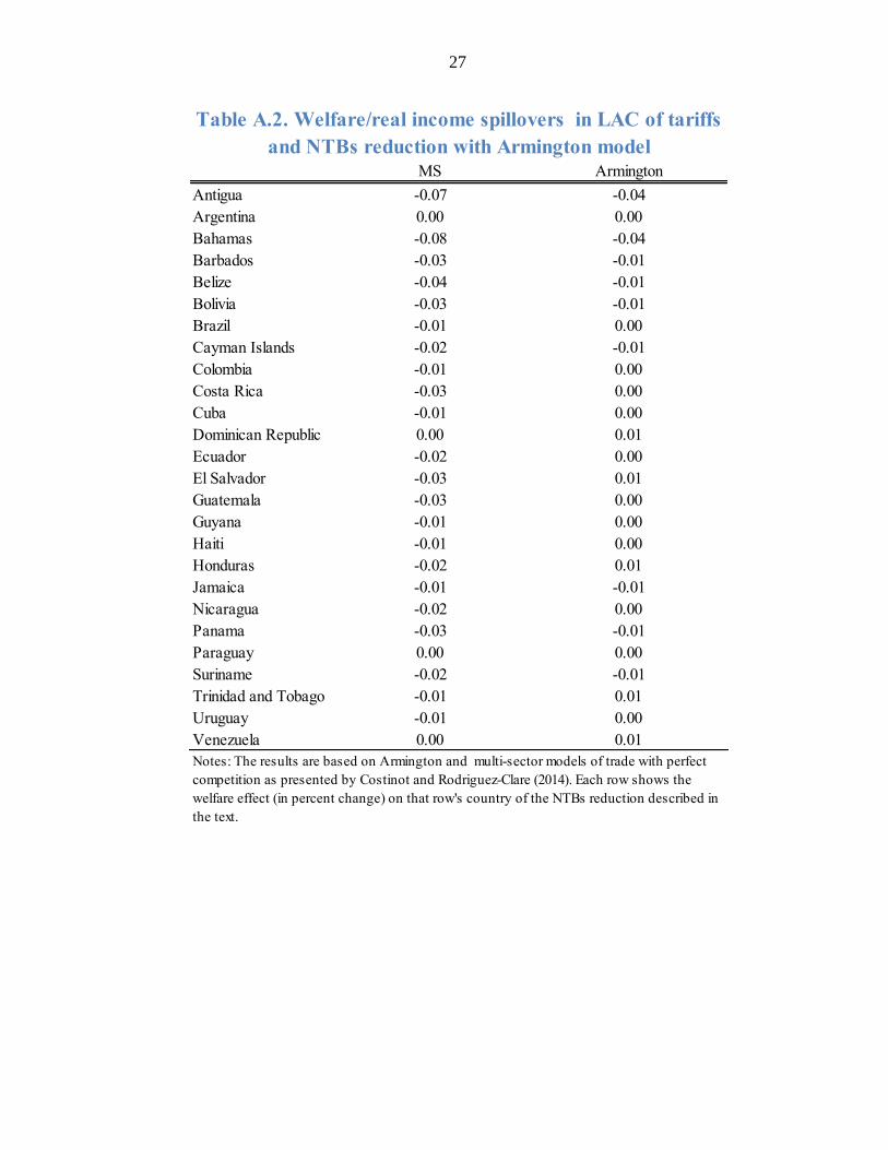
Tables A.1 and A.2 compare the results shown in the main text for the multi-sector (MS)

perfect competition model, with the ones obtained with the simpler Armington model. While

for most countries the results are roughly similar, larger discrepancies appear in the cases of

Singapore and Vietnam. Under the Armington model, these countries benefit by about 1 p.p.

more than in the MS model. This would favor the use of a multi-sector model where no

blanket assumption needs to be made on the elasticity of all sectors.

MS Armington

Australia 0.43 0.25

Brunei 0.34 0.49

Canada 0.27 0.22

Chile 0.33 0.13

Japan 0.17 0.13

Malaysia 3.58 3.82

Mexico 1.38 1.03

New Zealand 0.80 0.56

Peru 0.23 0.15

Singapore 1.70 2.77

USA 0.12 0.10

Vietnam 1.23 2.26

Table A.1. Welfare/real income effect of tariffs and NTBs

Notes: The results are based on Armington and multi-sector models of trade with perfect

competition as presented by Costinot and Rodriguez-Clare (2014). Each row shows the

welfare effect (in percent change) on that row's country of the NTBs reduction described

in the text.

reduction with MS and Armington model

27

MS Armington

Antigua -0.07 -0.04

Argentina 0.00 0.00

Bahamas -0.08 -0.04

Barbados -0.03 -0.01

Belize -0.04 -0.01

Bolivia -0.03 -0.01

Brazil -0.01 0.00

Cayman Islands -0.02 -0.01

Colombia -0.01 0.00

Costa Rica -0.03 0.00

Cuba -0.01 0.00

Dominican Republic 0.00 0.01

Ecuador -0.02 0.00

El Salvador -0.03 0.01

Guatemala -0.03 0.00

Guyana -0.01 0.00

Haiti -0.01 0.00

Honduras -0.02 0.01

Jamaica -0.01 -0.01

Nicaragua -0.02 0.00

Panama -0.03 -0.01

Paraguay 0.00 0.00

Suriname -0.02 -0.01

Trinidad and Tobago -0.01 0.01

Uruguay -0.01 0.00

Venezuela 0.00 0.01

Table A.2. Welfare/real income spillovers in LAC of tariffs

Notes: The results are based on Armington and multi-sector models of trade with perfect

competition as presented by Costinot and Rodriguez-Clare (2014). Each row shows the

welfare effect (in percent change) on that row's country of the NTBs reduction described in

the text.

and NTBs reduction with Armington model

28

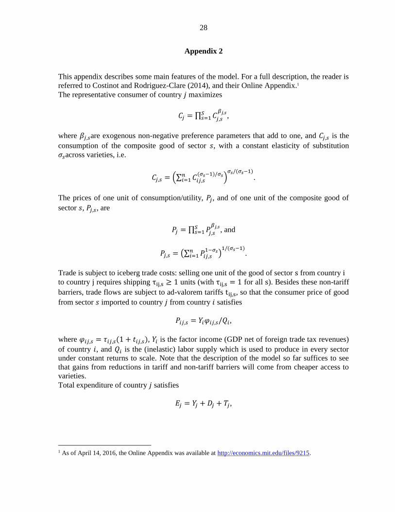
Appendix 2

This appendix describes some main features of the model. For a full description, the reader is

referred to Costinot and Rodriguez-Clare (2014), and their Online Appendix.1

The representative consumer of country 𝑗 maximizes

𝐶𝑗 = ∏ 𝐶𝑗,𝑠

𝛽𝑗,𝑠𝑆𝑠=1 ,

where 𝛽𝑗,𝑠are exogenous non-negative preference parameters that add to one, and 𝐶𝑗,𝑠 is the

consumption of the composite good of sector 𝑠, with a constant elasticity of substitution

𝜎𝑠across varieties, i.e.

𝐶𝑗,𝑠 = (∑ 𝐶𝑖𝑗,𝑠(𝜎𝑠−1)/𝜎𝑠𝑛

𝑖=1 )𝜎𝑠/(𝜎𝑠−1)

.

The prices of one unit of consumption/utility, 𝑃𝑗, and of one unit of the composite good of

sector 𝑠, 𝑃𝑗,𝑠, are

𝑃𝑗 = ∏ 𝑃𝑗,𝑠

𝛽𝑗,𝑠𝑆𝑠=1 , and

𝑃𝑗,𝑠 = (∑ 𝑃𝑖𝑗,𝑠1−𝜎𝑠𝑛

𝑖=1 )1/(𝜎𝑠−1)

.

Trade is subject to iceberg trade costs: selling one unit of the good of sector s from country i to country j requires shipping τij,s ≥ 1 units (with τij,s = 1 for all s). Besides these non-tariff

barriers, trade flows are subject to ad-valorem tariffs tij,s, so that the consumer price of good

from sector 𝑠 imported to country 𝑗 from country 𝑖 satisfies

𝑃𝑖𝑗,𝑠 = 𝑌𝑖𝜑𝑖𝑗,𝑠/𝑄𝑖,

where 𝜑𝑖𝑗,𝑠 = 𝜏𝑖𝑗,𝑠(1 + 𝑡𝑖𝑗,𝑠), 𝑌𝑖 is the factor income (GDP net of foreign trade tax revenues)

of country 𝑖, and 𝑄𝑖 is the (inelastic) labor supply which is used to produce in every sector

under constant returns to scale. Note that the description of the model so far suffices to see

that gains from reductions in tariff and non-tariff barriers will come from cheaper access to

varieties.

Total expenditure of country 𝑗 satisfies

𝐸𝑗 = 𝑌𝑗 + 𝐷𝑗 + 𝑇𝑗,

1 As of April 14, 2016, the Online Appendix was available at http://economics.mit.edu/files/9215.

29

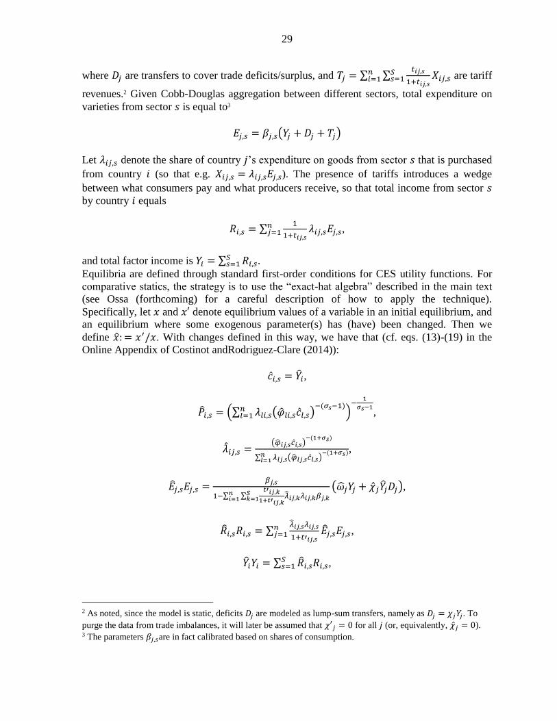
where 𝐷𝑗 are transfers to cover trade deficits/surplus, and 𝑇𝑗 = ∑ ∑𝑡𝑖𝑗,𝑠

1+𝑡𝑖𝑗,𝑠𝑋𝑖𝑗,𝑠

𝑆𝑠=1

𝑛𝑖=1 are tariff

revenues.2 Given Cobb-Douglas aggregation between different sectors, total expenditure on

varieties from sector 𝑠 is equal to3

𝐸𝑗,𝑠 = 𝛽𝑗,𝑠(𝑌𝑗 + 𝐷𝑗 + 𝑇𝑗)

Let 𝜆𝑖𝑗,𝑠 denote the share of country 𝑗’s expenditure on goods from sector 𝑠 that is purchased

from country 𝑖 (so that e.g. 𝑋𝑖𝑗,𝑠 = 𝜆𝑖𝑗,𝑠𝐸𝑗,𝑠). The presence of tariffs introduces a wedge

between what consumers pay and what producers receive, so that total income from sector 𝑠

by country 𝑖 equals

𝑅𝑖,𝑠 = ∑1

1+𝑡𝑖𝑗,𝑠𝜆𝑖𝑗,𝑠𝐸𝑗,𝑠

𝑛𝑗=1 ,

and total factor income is 𝑌𝑖 = ∑ 𝑅𝑖,𝑠𝑆𝑠=1 .

Equilibria are defined through standard first-order conditions for CES utility functions. For

comparative statics, the strategy is to use the “exact-hat algebra” described in the main text

(see Ossa (forthcoming) for a careful description of how to apply the technique).

Specifically, let 𝑥 and 𝑥′ denote equilibrium values of a variable in an initial equilibrium, and

an equilibrium where some exogenous parameter(s) has (have) been changed. Then we

define �̂�: = 𝑥′/𝑥. With changes defined in this way, we have that (cf. eqs. (13)-(19) in the

Online Appendix of Costinot andRodriguez-Clare (2014)):

�̂�𝑖,𝑠 = �̂�𝑖,

�̂�𝑖,𝑠 = (∑ 𝜆𝑙𝑖,𝑠(�̂�𝑙𝑖,𝑠�̂�𝑙,𝑠)−(𝜎𝑠−1)𝑛

𝑙=1 )−

1

𝜎𝑠−1,

�̂�𝑖𝑗,𝑠 =(�̂�𝑖𝑗,𝑠𝑐̂𝑖,𝑠)

−(1+𝜎𝑠)

∑ 𝜆𝑙𝑗,𝑠(�̂�𝑙𝑗,𝑠𝑐̂𝑙,𝑠)−(1+𝜎𝑠)𝑛

𝑙=1

,

�̂�𝑗,𝑠𝐸𝑗,𝑠 =𝛽𝑗,𝑠

1−∑ ∑𝑡′𝑖𝑗,𝑘

1+𝑡′𝑖𝑗,𝑘�̂�𝑖𝑗,𝑘𝜆𝑖𝑗,𝑘

𝑆𝑘=1

𝑛𝑖=1 𝛽𝑗,𝑘

(�̂�𝑗𝑌𝑗 + �̂�𝑗�̂�𝑗𝐷𝑗),

�̂�𝑖,𝑠𝑅𝑖,𝑠 = ∑�̂�𝑖𝑗,𝑠𝜆𝑖𝑗,𝑠

1+𝑡′𝑖𝑗,𝑠

𝑛𝑗=1 �̂�𝑗,𝑠𝐸𝑗,𝑠,

�̂�𝑖𝑌𝑖 = ∑ �̂�𝑖,𝑠𝑅𝑖,𝑠𝑆𝑠=1 ,

2 As noted, since the model is static, deficits 𝐷𝑗 are modeled as lump-sum transfers, namely as 𝐷𝑗 = 𝜒𝑗𝑌𝑗. To

purge the data from trade imbalances, it will later be assumed that 𝜒′𝑗 = 0 for all 𝑗 (or, equivalently, �̂�𝑗 = 0). 3 The parameters 𝛽𝑗,𝑠are in fact calibrated based on shares of consumption.

30

∑ �̂�𝑖𝑌𝑖 = 1𝑛𝑖=1 ,

where the last equation comes from world GDP being numeraire in all equilibria. The model

is solved by using the interior point algorithm, maximizing a constant function subject to the

constraint that all “hat” equations above are satisfied.