estimating terrain elevation maps from sparse and ... they do not address fusion of data from...
TRANSCRIPT

Estimating Terrain Elevation Maps from Sparse
and Uncertain Multi-Sensor Data
Dominik Belter, Przemysław Łabecki, Piotr Skrzypczynski
Abstract— This paper addresses the issues of unstructuredterrain modelling for the purpose of motion planning in aninsect-like walking robot. Starting from the well-establishedelevation grid concept adopted to the specific requirementsof a small legged robot with limited perceptual capabilitieswe extend this idea to a multi-sensor system consisting ofa 2D pitched laser scanner, and a stereo vision camera. Wepropose an extension of the usual, ad hoc elevation grid updatemechanism by incorporating formal treatment of the spatialuncertainty, and show how data from different sensors canbe fused into a consistent terrain model. Moreover, this paperdescribes a novel method for filling-in missing areas of theelevation grid, which appear due to erroneous data or theline-of-sight constraints of the sensors. This method takes intoaccount the uncertainty of the multi-sensor data collected inthe elevation grid.
I. INTRODUCTION
Over millions of years Nature has brought legged locomo-
tion near to perfection. Also walking machines can cope well
with the lack of roads and rugged terrain. However, despite
major achievements in the past years, walking robots cannot
compete with wheeled and tracked robots concerning their
autonomy. A high level of autonomy can be achieved only
if the robot perceives the surrounding terrain and plans its
motion on the basis of a terrain map. The classic 2D maps are
insufficient for walking robots, they need an representation
of the terrain elevation in order to plan the body path, the
trajectories of the legs, and the footholds. Such a map can
be constructed from the sensory data in the form of an
elevation grid, which is a 2.5D tessellated representation of
the surrounding terrain. Elevation grids were conceived for
early outdoor robots with 3D laser sensors [12]. In these
maps each cell contains a value that represents the height of
the terrain at that cell. A particular variant of this concept
was adopted for a wheeled vehicle equipped with an inclined
2D laser scanner Sick LMS 200 as the terrain sensor [19]. In
this case the sparse range readings have to be registered in
a grid using an estimate of the robot motion (Fig. 1A). The
inclined 2D laser scanner is of particular interest for small
walking robots, like our Messor hexapod (Fig. 1B), because
such robots cannot carry bigger and heavy 3D laser scanners.
Note that we consider only the terrain mapping problem, not
Simultaneous Localization and Mapping (SLAM), thus we
assume that an accurate estimate of the robot pose in 6-d.o.f
is available. For the real robot this estimate is provided by the
The authors are with the Institute of Control and Information En-gineering, Poznan University of Technology, ul. Piotrowo 3A, PL-60-965 Poznan, Poland. [email protected], [email protected], pi-
vision-based Parallel Tracking and Mapping (PTAM) pose
tracking algorithm running in parallel to terrain mapping [4].
A
d(2
6 c
m)
z
a=45o
Ym
Ys
ZmZs
B
d(4
8 c
m)
zk
a=35o
Fig. 1. Configuration of the multi-sensor terrain perception system (A),and Messor with this system traversing unstructured terrain (B)
The basic terrain mapping algorithm used on the Messor
robot was detailed in our previous work [2]. This algorithm
is an adaptation of the Ye and Borenstein’s method [19], but
is more suitable to a walking robot with the compact Hokuyo
URG-04LX laser scanner. The obtained map is used for
efficient foothold planning [2]. However, to efficiently plan
the robot’s body path while perceiving the terrain, a sensory
system with much longer range than the pitched URG-04LX
is needed. We employ the Videre Design STOC (STereo On
a Chip) passive stereo vision camera, which yields a dense
depth map in real-time, owing to the hardware-embedded
image processing. Unfortunately, the STOC camera range
data are sparse and corrupted by various artefacts.
Taking the limitations of the above-mentioned sensors into
account we conceived a dual-grid elevation map [3], which
employs a small, precise grid that surrounds the robot and is
updated from all the range data available to the robot, and
a bigger grid describing the more distant areas, perceived
only by means of the STOC camera. However, in [3] the
data from stereo vision and 2D laser were fused by ad
hoc rules, which didn’t take advantage of the uncertainty
models of the particular sensors. In this paper we present
a more rigorous treatment of the spatial uncertainty for
elevation map estimation. We also try to cope with the
sparseness of the available data employing a Gaussian-based
approximation method to fill-in discontinuities that appear in
the elevation grid.
II. RELATED WORK
Some of the grid-based algorithms for rough terrain
mapping use ad hoc formulations for sensor fusion, e.g.
Ye and Borenstein [19] apply some heuristics when they
fuse consecutive laser range measurements into an elevation
grid: their certainty measure is a simple hit/miss counter,
978-1-4673-2126-6/12/$31.00 © 2012 IEEE

and they do not address fusion of data from different
sensors, focusing on the Sick LMS 200 scanner. On the
other hand, there are 2.5D mapping methods, which are
based on probabilistic foundations. The locus method of [12]
applies simple geometric approximation in order to obtain
elevation uncertainty from the sensor error model. This
approximation, however, does not account for the uncertainty
of measurements. Recently, a method for efficient volumetric
mapping was presented, which employs the notion of positive
and negative occupancy mass to represent the environment
[6]. Although this model is efficient with regard to the map
size, it is rather suited for robots that require full 3D world
model, not for walking robots, which can use much simpler
surface maps.
An entirely different concept is presented in [16], where a
non-parametric continuous surface estimation method is pro-
posed. This method is based on Gaussian process regression
and applies non-stationary covariance functions for adapta-
tion of the regression kernels to the structure of the terrain.
It enables filling-in large gaps in elevation data, and provides
estimates of uncertainty for the filled-in regions. However,
these advantages come at the cost of high computational
burden, which can be prohibitive for a small walking robot.
Stereo vision was used for terrain modelling with walking
robots in few projects, mostly because typical stereo systems
impose high costs of 3D points computation. In [9] and [17]
walking robots with stereo-based perception are shown to
traverse autonomously rugged terrain, but in both cases the
computations are done off-board, and there is no explicit
propagation of the spatial uncertainty from the stereo data to
the elevation map.
So far we do not extend our mapping system towards
description of multi-level or overhanging objects, such as
bridges and tunnels. This can be implemented with the multi-
level surface maps, as described in [15], but it is not applica-
ble to the sensing system of the Messor walking robot, which
uses pitched sensors that cannot perceive high/overhanging
objects.
III. SENSORS AND SPATIAL UNCERTAINTY
A. Compact 2D laser scanner as a terrain sensor
The Hokuyo URG-04LX scanning rangefinder exploits the
phase-shift-based ranging principle. The default angular res-
olution is 0.352◦with 683 range readings per scan. According
to the manufacturer the URG-04LX scanner measures ranges
up to 1 m with the accuracy of 10 mm, and ranges between
1 and 4 m with the accuracy of 1% of the measured distance,
but this specification is valid only for a white sheet of paper.
The extended control protocol SCIP 2.0 makes it possible
to obtain also the received intensity values, and the AGC
(Automatic Gain Control) voltage. However, the SCIP 2.0
intensity/AGC scanning mode has smaller angular resolution
of 1.056◦.
The URG-04LX scanner suffers from a strong dependency
between the accuracy of the range measurements and the
optical properties of the target surface because of the used
ranging principle. The consequences of this fact are twofold:
(i) some black or shiny surfaces do not provide valid range
measurements; (ii) an universal calibration model is difficult
to establish without the knowledge of the target surface
properties (Fig. 2A). Most of the corrupted measurements
can be rejected on the basis of very weak intensity values
being received by the sensor. Because the intensity I that
can be read from the sensor depends on the AGC values, we
use the formula
Ires =
√I · 1023vAGC
, (1)
to obtain the restored intensity [8]. In (1) vAGC is the AGC
voltage, and 1023 is the range of the 10-bit A/D converter
used in the sensor. The values of restored intensity we
observed in our experiments were between 40 and 320 for
distances up to 2 m. On the basis of results of experiments
with various surfaces (wood, black plastic, concrete) we set
the reliable measurement intensity threshold at Ires = 100
for targets closer than 1 m, i.e. within the field of view of
our pitched URG-04LX scanner.
-6
-5
-4
-3
-2
-1
0
1
3
0 10 20 30 40 50 60 70 80 90 100
white paint
black paint
concrete
wood (light)
grey paint
0 10 20 30 40 50 60 70 80 90 1000.5
1
1.5
2
2.5
3
3.5
4
4.5
5
white paint
black paint
concrete
wood (light)
grey paint
measured distance [cm] measured distance [cm]
measure
ment err
or
[mm
]
sta
ndard
devia
tion [m
m]
A B2
Fig. 2. Calibrated range measurements for five different target surfaces (A),and the dependency between the range standard deviation and the measureddistance (B)
Rigorous modelling of measurement uncertainty, e.g. ob-
taining the variance of the measured ranges is problematic
for the compact scanner under study. As shown by others
[10] the standard deviations observed for URG-04LX mea-
surements are small even for large absolute errors in the
measured distance. Our experiments show that there is also
no clear dependency between the intensity output and the
observed standard deviation. Therefore, the method for esti-
mating the range variance in a phase-shift-based range finder
upon the known intensity output proposed in [1] cannot be
applied here. Eventually, we take a rough but conservative
approximation of the range errors. We used experimental
data for measured distances from 50 to 1000 mm with five
different surfaces and the incidence angle of 30◦. We picked
the largest standard deviation for every measured distance,
and then established a mathematical model that approximates
the change of the range standard deviation σr as function of
the measured range. The approximated curve shown as the
solid line in Fig. 2B gives standard deviation values larger
than most of the used actual measurements (shown as small
circles), only errors of measurements from a black-painted
surface are slightly underestimated.
For updating the terrain map each range rs measured at
the bearing angle β of the laser scanner is transformed to
the elevation grid coordinates psm by using the robot pose

estimate:
psm =
xm
ymzm
= Tms
rs sinβrs cosβ
0
, (2)
where the homogeneous matrix Tms defines the transforma-
tion from the laser scanner frame to the coordinates of the
grid. This transformation depends on the pose of the walking
robot, as the laser scanner is rigidly attached to the robot’s
body (see [2] equations 2 and 3).
Prior to integration with the terrain map, range mea-
surements from the URG-04LX sensor are checked for
validity against the restored intensity values, and then mixed
measurements are eliminated by the clustering algorithms
detailed in [2].
The spatial uncertainty of a point psm, given by the Cs
pm
covariance matrix depends on two independent factors: the
uncertainty of the range measurement, and the uncertainty
of the robot pose:
Cpsm=
σ2x σxy σxz
σxy σ2y σyz
σxz σyz σ2z
= JRSCR(k)JTRS+JSCSJ
TS ,
(3)
where JRS and JS are the Jacobians of (2) with respect
to (w.r.t) xR and rs, respectively, CR(k) is the covariance
matrix of the 6-d.o.f robot pose at the k-th time instant
when the range measurement was obtained, and CS is the
range measurement covariance matrix, which reduces to the
range variance σ2r , because we assume (as in [1]) that the
bearing angle β is known perfectly. The σ2z taken from (3) is
the uncertainty of the measured elevation. Thus, ∆z = 3σz
captures the true elevation with 99.7% probability, and can
be used as a convenient measure of the sensing system
precision.
B. Long-range perception with stereo vision
The Videre Design STOC camera implements in its
hardware the Small Vision System (SVS) algorithm [11],
which uses correlation-based matching on rectified images,
producing a dense depth map. The camera software outputs
disparity images, or alternatively, point clouds. The stereo
camera often produces incorrect matches. Errors occur as
a result of insufficient image texture and around depth
boundaries or when objects are too close to the camera.
The artefacts on the borders of objects with disparity values
much different from the background manifest themselves as
halos stretched from the foreground to the background object.
Other artefacts, such like out-of-horopter measurements and
measurements in texture-less areas manifest themselves as
groups of points near the camera. In [13] we show how to
remove the artefacts belonging to both groups by analyzing
the depth image.
The most obvious causes of measurement errors in stereo
vision are finite image resolution and false matches. Because
the matches are performed on rectified images and the
rectification algorithm uses a calibrated camera model, the
uncertainty of calibration also contributes to the overall
measurement uncertainty. Matching errors are, due to their
random nature, difficult to determine and they are not con-
sidered in the following analysis.
The camera model used by the rectification algorithm com-
prises of a standard pinhole camera model and a distortion
model that includes barrel distortion (modeled using a sixth-
degree polynomial), and tangential distortion. To rectify the
images, the extrinsic parameters of the stereo system are
also needed. A total of 24 parameters are estimated by the
calibration of a stereo system. The calibration uncertainty
can then be propagated through the rectification and 3D
coordinate calculation equations to estimate the uncertainty
of measured 3D coordinates.
Because in practice undistortion is performed by choosing
a fixed position on the undistorted image and performing
distortion to determine the corresponding position on the
distorted image, linearised equations for xu and yu are used:
xu = g1(ud, vd, k1, k2, k3, p1, p2, fx, fy, cx, cy)yu = g2(ud, vd, k1, k2, k3, p1, p2, fx, fy, cx, cy)
, (4)
where ud and ud are the pixel coordinates on the distorted
image, and xu and yu are the corresponding undistorted co-
ordinates, while k1, k2, k3, p1, p2 are distortion coefficients,
and fx, fy, cx, cy are intrinsic parameters of the camera.
Equations relating the undistorted camera coordinates and
the rectified pixel coordinates are in the form of:
ur = h1(xu, yu, Tx, Ty, Tz, θx, θy, θz, frx, fry, crx, cry)vr = h2(xu, yu, Tx, Ty, Tz, θx, θy, θz, frx, fry, crx, cry)
,
(5)
where ur and vr are the coordinates of the pixel in the
rectified image, xu and yu are the corresponding camera
coordinates in the undistorted image, Tx, Ty, Tz, θx, θy, θzare the extrinsic parameters of the stereo vision system and
frx, fry, crx, cry are the intrinsic parameters for the rectified
image.
The propagation of calibration uncertainty through the
undistortion equations can be calculated as follows:
Cu = JuCdJTu , (6)
where Ju is the Jacobian of (4) w.r.t all the parameters
excluding ud and vd, which are assumed fixed, Cd is the
covariance matrix containing the variances of calibration
parameters, and Cu is the resulting 2×2 covariance matrix of
the undistorted coordinates. The propagation of uncertainty
through the rectification equations is performed in a similar
way:
Cr = JrCueJTr , (7)
where Jr is the Jacobian of (5) w.r.t
xu, yu, Tx, Ty, Tz, θx, θy, θz , and Cue is the 8×8 covariance
matrix of undistorted coordinates and extrinsic parameters
of the camera, while Cr is the 2×2 covariance matrix of
the pixel coordinates on the rectified image.
The calculation of the 3D coordinates is two-step. In
the first step, depth is calculated from disparity, using the
equation:
zc =Trxfr
d, (8)

where d is the disparity value at the given depth, fr is the
focal length of the rectified image (fr = fry = frx). Trx
is the distance from the left camera to the right camera,
and is equal to the position along the x axis of the right
camera in the left camera rectified coordinate system. In the
second step, xc and yc coordinates are calculated, given the
depth and the corresponding pixel coordinates in the rectified
image:
xc =(vr − cxr)
frzc, yc =
(ur − cyr)
frzc, (9)
where, vr and ur are pixel coordinates in the rectified image,
and cxr, cyr fr are the intrinsic parameters for the rectified
image.
It is assumed, that the uncertainty of the pixel location
in the v axis has no effect on row alignment (which would
hinder correct matching), and therefore does not affect the
calculated depth. However, the uncertainty of the pixel
location in the u axis (on both left and right images) creates
disparity uncertainty and propagates to depth uncertainty.
The disparity uncertainty is calculated as σd = σul+ σur
,
where σd is the standard deviation of the disparity, while
σurland σurr
is the standard deviation of the location of the
pixel along the u axis in the left and right rectified images.
The covariance matrix Cpcof a 3D point in the camera
coordinates pc = [xcyczc]T is calculated as:
Cpc= JpCrpJ
Tp . (10)
Jp is the Jacobian of (8) and (9) w.r.t d, ur and vr, while
Crp is the covariance matrix for d, ur and vr. Then, the
coordinates of a point in the map are calculated
pcm =
xm
ymzm
= Tms T−1
cs pc, (11)
where Tcs is the homogeneous matrix of the transformation
from the laser scanner to camera coordinate system. As the
scanner-camera mounting is rigid, we assume that the off-line
calibration [14] is precise enough to neglect its uncertainty.
Therefore the uncertainty of a point in the map coordinates
is given by:
Cpcm=
σ2x σxy σxz
σxy σ2y σyz
σxz σyz σ2z
= JRCCR(k)JTRC+JCCpc
JTC ,
(12)
where JRC and JC are the Jacobians of (11) w.r.t xR and
pc, respectively, CR(k) is the covariance of the robot pose
at the moment the stereo measurement was made.
-0.5 -0.4 -0.3 -0.2 -0.1 0 0.1 0.2 0.3 0.4 0.50
0.1
0.2
0.3
z[m
]
x [m]
estimated profile
real profile
uncertainty boundaries
Fig. 3. Profile of an example elevation map with visualization of the ∆z
elevation uncertainty boundaries
The σz value computed from (12) is the uncertainty of the
measured elevation, while ∆z = 3σz defines the elevation
confidence interval. Figure 3 shows that this interval defined
w.r.t the estimated profile (blue line) of a rocky terrain
mockup mapped from the STOC sensor data captures the
ground truth profile (red line) of the mockup.
IV. TERRAIN MAPPING METHOD
A. Elevation map concept
In perception-based walking the crucial problem is
foothold selection, because any wrongly positioned step can
result in falling down [2]. The foothold selection algorithm
requires a high resolution elevation map, which captures
geometry of the terrain at the scale of the robot foot size. It
is not possible to obtain such a map from the STOC camera
range data, but it can be created by registering the sparse
range data from the pitched laser scanner in a local grid.
In the current implementation on the Messor robot the local
grid with cells of 15×15 mm is used.
-300
-200
-100
0
100
200
300-300
-200
-100
0
100
200
larger elevation grid
local elevation grid
300
single cell of theelevation grid
singleelevation bin p
ossib
leele
vation v
alu
es
alternativeelevation
hypothesis
currentelevation
(winning bin)
Fig. 4. Concept of the elevation map with multi-bin cells
Its maximal dimensions are 2×2 m, according to the range
of the pitched scanner. Range data from the STOC camera
allow to create a bigger, but less precise elevation grid. The
larger map size is 10 × 10 m, as the STOC camera can
perceive objects at distances up to 5 m. Such a map can
be used for robot’s body path planning, but is not precise
enough for foothold selection, due to the limited precision
of the range data from stereo at larger distances. The centres
of the two maps are co-located at the origin of the robot
coordinate system (Fig. 4). As the robot moves, both maps
are translated to cover new areas. Therefore the robot always
has a precise map of the terrain in its closest neighborhood,
and a rough map of the more distant areas. Although the
larger elevation grid is constructed only from stereo range
measurements, and the smaller precise grid is updated mostly
by the URG-04LX range data, the area covered by the precise
grid overlaps with the area that was already observed by the
stereo camera and mapped in the rough map. Therefore, the
two maps need to be compatible w.r.t the representation of
the elevation values, and there should be a mechanism that
enables fusion of the data, taking into account uncertainty of
the elevation obtained from both sensors.

B. Elevation updating algorithm
The URG-04LX scanner requires the motion of the robot
to obtain 3D data. Therefore, we developed an elevation grid
updating method, which is based upon the Ye and Borenstein
concept [19], and our extension of this concept tailored
specifically for walking robots, as described in [2]. However,
the new version for multi-sensor perception uses probabilistic
mechanisms for data fusion. The ad hoc formulation of
hit/miss certainty values is applied only to identify grid cells
that received too few range readings, while estimation of the
elevation values employs Kalman filtering.
In [19] and in our previous works [2], [3] the terrain map
data structure consists of two 2D grids of the same size –
one for elevation, and one for certainty. Here we extend this
structure by dividing the space corresponding to each cell
into vertically arranged bins of equal height (50 mm in the
current implementation). Therefore, a cell in the elevation
map is denoted as h[i,j,n], and a cell in the certainty map
as c[i,j,n], where i, j are indices of the cells, and n is the
bin index starting from the zero level (thus, n can be also
negative).
At every time instant new elevation measurements from
both sensors are registered in particular bins depending on
their hm = zm + dz + href value, where dz is the height of
the sensor (cf. Fig. 1A, note that different values are used for
measurements from both sensors), and href is the elevation
at which the robot is located. The bin that contains the most
points from new measurements is used to calculate the new
elevation value in the given cell, and only this elevation is
used for motion planning. Although only one bin is selected,
the measurements associated to other bins are not discarded
(Fig. 4).
The certainty value of each cell/bin counts the number of
measurements from both sensors associated to this cell/bin.
A single elevation measurement from stereo updates the
certainty according to the formula:
c[i,j,n](k+1) =
{
c[i,j,n](k) + a if ∆z ≤ ∆max
c[i,j,n](k) otherwise,
(13)
where a is constant increment of the certainty, ∆z is the
99.7% probability interval of the elevation measurement, and
∆max is the maximum elevation uncertainty allowed for the
elevation. For the laser scanner measurements this formula
is more complicated. The 2D sensor uses the robot motion
to scan the terrain, thus we apply the constraints on motion
continuity proposed in [19] to the range data in order to
further eliminate spurious measurements:
c[i,j,n](k+1) =
c[i,j,n](k) + a if (∆z ≤ ∆max and
∣
∣
∣hm(k+1) − h
[i,j,n](k)
∣
∣
∣≤
∣
∣∆zmax(k)
∣
∣
)
or c[i,j,n](k) = 0
c[i,j,n](k) otherwise,
(14)
where ∆zmax(k) is a prediction of the maximum change
of elevation between two consecutive measurements, which
is computed taking into account the maximum range mea-
surement error, and errors in the robot pose estimate. The
computations of ∆zmax(k) for a walking robot are detailed
in [2], and omitted here due to the lack of space.
Once the most certain bin for each updated cell of the
grid is determined, the elevation estimate is computed upon
the collected measurements. To this end an one-dimensional
static Kalman filter is applied, which fuses all the individual
hm elevations obtained from the vertical coordinates of the
pm points accumulated in the bin, with the σ2z values of the
points used as weights:
K = σ2[i,j,n]h(k)
(
σ2[i,j,n]h(k) + σ2
z(k+1)
)
−1
,
h[i,j,n](k+1) = h
[i,j,n](k) −K
(
h[i,j,n](k) − hm(k+1)
)
, (15)
σ2[i,j,n]h(k+1) = (1−K)σ
2[i,j,n]h(k) ,
where K is the Kalman gain, σ2h is the variance of the
elevation stored in the given cell/bin, and h[i,j,n](k+1) is the
updated elevation value. Note that k is iterated w.r.t the time
instances at which the range measurements were collected,
and that (15) can be updated asynchronously from the laser
scanner (which is faster) and the stereo camera. The Kalman
filter fuses old elevation data (already in the map) and
new elevation data from the laser scanner and stereo vision
in an optimal way. This procedure is applied not only to
the “winning” bin, but also to other bins containing valid
elevation data (i.e. the certainty of the bin is greater than
zero). This way we maintain several alternative elevation
hypotheses, avoiding making irreversible decisions upon few
range measurements.
A B
Fig. 5. Application of visibility constraints – an example. Fragment of amap built without evaluation of visibility (A), fragment of a map with thevisibility constraint used (B)
One last step in the elevation map updating is application
of the visibility constraint. If new data contain discontinu-
ities, old but erroneous elevations can be retained in such
gaps. Checking the visibility constraints helps to remove
these elevations. Each cell, which was not updated in the
last measurement cycle is checked whether it occludes newly
modified cells. If the certainty of the cells in the gap is lesser
than of the occluded cells, the measurements in the gap are
removed. If the updated cell contains more than one bin with
measurements, then the conflicting bin is invalidated (cer-
tainty decreased by a fixed amount), automatically making
the next-best elevation hypothesis the valid elevation of that
cell.
The simple elevation updating formula used in [19] and
adopted in [2] did not allow the stored elevation values to de-
crease. This approach was justified for range measurements
from the tilted down 2D scanner, which measured most of
the cells representing flat terrain only once. However, the
multi sensor system needs a way to remove some wrong
elevations stored already in the map from the noisy stereo
measurements. Another advantage of the current formulation
of the elevation updating rule is that the map can accommo-
date changes in the terrain, providing that they are slow.
C. Approximation of empty areas in the map
Valid elevation estimates with uncertainty reside only in
the cells that were observed at least once by at least one
of the two sensors. Because of the line-of-sight constraints
of the pitched sensors, and because of the empty areas in
the stereo data, gaps appear in the elevation grid. They are
usually small (of few cells size) in the local grid updated
from the laser data, but they can be much larger in the map
constructed only from the stereo data. Therefore, a procedure
is needed to fill-in the missing data in the elevation map.
Small gaps in the local map are efficiently filled-in by the
Weighted Median Filter proposed in [19], which applies a
filter skeleton to a 5×5 window in the elevation grid. The
skeleton has bigger weights for cells farther from the center
of the window, because these cells more likely contain highly
certain elevation values. The median filter considers only
the bins with the highest certainty value in the neighboring
cells. As proposed in [2], the output hwm of the WM filter
is assigned to each cell in the local map, which was never
updated (c[i,j,n]=0 for all n). The computed elevation value
is stored in a proper bin of the filled-in cell, however the
certainty value is not updated, which allows the foothold
selection procedure to avoid such unknown areas, if possible.
Unlike the original formula of [19] our filling-in rule newer
sets the elevations to zero in the areas of low certainty. The
elevation standard deviation in a filled-in cell is computed
as the weighted average of the standard deviations from the
neighboring cells, using the same filter skeleton. This makes
the computed spatial uncertainty consistent with that of the
neighboring cells.
Large gaps at self-occluded areas of the local map and
holes in featureless parts of the larger map from stereo data
cannot be filled by the simple median filtering. Therefore, we
try to approximate the elevation values in these areas from
the elevation data available at neighboring locations using
the technique based on multi-dimensional Gaussians, which
we originally conceived for approximation of the decision
surface in the foothold selection problem of the walking
robot [2]. In this procedure for each cell in the elevation map
again only the bin with the highest certainty value is used.
The estimated elevation hm is treated as an unknown func-
tion of the elevation grid coordinates (i, j). This function is
approximated by a polynomial, which structure is suggested
by the generalized form of the Kolmogorov theorem [5].
hm(i, j) =
m∑
q=0
cq · exp(
λ1,q(i− a1,q)2 + λ2,q(j − a2,q)
2)
.
(16)
Sums of radial basis functions are often used to approximate
given functions. Similarly, in (16) two-dimensional Gaussian
functions are used, which are shaped to follow the available
elevation data by the parameters λi,q and ai,q , with i = 1, 2and q = 0, . . . ,m, where m represents complexity of the
approximated model, and is determined automatically by
using the Akaike Information Criterion [18]. The vector of cqcoefficients can be efficiently computed from Least-Squares
Fitting using the Gram matrix [2]. However, finding λi,q
and ai,q is an optimization problem. Because there is no
analytical model of the dependencies between the sought
variables, a general, population-based optimization method
is used to find optimal values of λi,q and ai,q , namely the
Particle Swarm Optimization (PSO) [7]. The fitness function
in PSO is the squared Mahalanobis distance between the
training points (i.e. known elevations in the grid cells) and
the corresponding points of the obtained surface. Using the
Mahalanobis distance allows to account for the elevation
uncertainty. The approximated surface adheres more to less
uncertain data. The procedure results in a close-form function
that can be later used to compute elevations at arbitrary cells
of the approximated area. Although the PSO method usually
finds the parameters in (16) in few iterations, the large
number of training points in the whole elevation grid results
in runtimes of several minutes, which are unacceptable in the
control system of the robot. Therefore, we apply (16) only
to separated areas around large empty spaces in the elevation
map. These areas are identified by examining the certainty
map, which holds zeros for gaps in the elevation map.
Square patches (called support areas) are defined around the
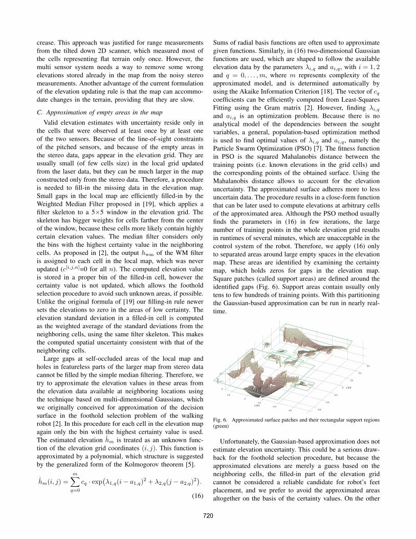
identified gaps (Fig. 6). Support areas contain usually only
tens to few hundreds of training points. With this partitioning
the Gaussian-based approximation can be run in nearly real-
time.
-0.6
-0.4
-0.2
0
0.2
0.4
0.6
-0.6
-0.4
-0.2
0
0.2
0
0.1
0.2
x [m]
y [m]
z [m
]
Fig. 6. Approximated surface patches and their rectangular support regions(green)
Unfortunately, the Gaussian-based approximation does not
estimate elevation uncertainty. This could be a serious draw-
back for the foothold selection procedure, but because the
approximated elevations are merely a guess based on the
neighboring cells, the filled-in part of the elevation grid
cannot be considered a reliable candidate for robot’s feet
placement, and we prefer to avoid the approximated areas
altogether on the basis of the certainty values. On the other

hand, the approximated areas are important for the A⋆-based
path planning procedure [3], which does not consider the
uncertainty of individual elevations.
V. EXPERIMENTS AND RESULTS
The mapping system was tested in a controlled envi-
ronment using a rugged terrain mockup of size 150×150
cm. The supporting pylon with the URG-04LX scanner
and STOC camera from the Messor robot was attached
to the wrist of the KUKA KR-200 industrial robot, which
simulated the motion of the walking machine. Owing to this
experimental setup we had “perfect” self localization, thus
making the tests independent from the robot pose estimate
errors and focusing on the performance of the exteroceptive
sensors. The sensors were moved in equal intervals towards
the mockup, and in each position measurements with both
of them were made.The use of an industrial robot made the
motion trajectories repeatable, to test different configurations
of the sensors. The ground truth (Fig. 7A) was obtained
by densely scanning the terrain mockup with a vertically
positioned laser scanner to avoid self-occlusions.
The presented approach to elevation mapping is compared
with our old method described in [2] in a quantitative way
by using a variant of the Performance Index (PI), originally
introduced in [19]. As the ability to fill-in gaps in the map is
one of the important improvements in the presented method,
we modified the PI to account for missing elevation values.
To compute PI we use the equation:
PI =
∑n
i=1
∑m
j=1 o[i,j]f
(
h[i,j]f − h
[i,j]t
)2
∑n
i=1
∑m
j=1 o[i,j]r
(
h[i,j]r − h
[i,j]t
)2 ·Nr
Nf
, (17)
where n and m define the size of the map, while i and j are
coordinates of the point in the grid. Note that PI is computed
for 2D grids, so we take the elevation values from the most
certain bins of our map. The formula (17) compares the
elevations h[i,j]f in the grid built with a mapping algorithm,
either the old one from [2] or the one presented here, with
the elevation values h[i,j]r obtained by simply registering the
range data (either laser or stereo) in the grid, and the ground
truth map elevations h[i,j]t . The number of valid elevation
cells (c[i,j,n] > 0 for some n) in the map build with the given
mapping method, and in the raw elevation map is given by
Nf and Nr, respectively. The coefficients o[i,j]f and o
[i,j]r can
be either zero or one – they determine if the given cell has
a valid elevation value.
The result of (17) tells how much the given mapping
method reduces elevation errors w.r.t a raw elevation map.
Better reduction of errors causes lower PI values. Results of
these tests are shown in Fig. 8, which plots the PI values for
the elevation map obtained from the URG-04LX laser data
(intensity/AGC mode, Fig. 7B) integrated according to the
method of [2] (red bar).
Improved elevation maps can be obtained by exploiting the
restored intensity values in order to eliminate spurious laser
range measurements, and by integrating the laser and stereo
A
B
C
D
Fig. 7. Maps of a terrain mockup: ground truth (A), elevation map fromlaser data (B), elevation map fusing laser and stereo data (C), elevation mapwith gaps filled-in by the Gaussian approximation (D)
laser
data
old
meth
od
Perf
orm
ance
Index (
PI)
maps from Fig. 7
fused d
ata
no g
ap fill
ing
fused d
ata
Gaussia
n a
ppro
x.
Fig. 8. PI values obtained in the controlled environment experiments
vision data according to the presented method (Fig. 7C).
Further improvement w.r.t the reduction of gaps is achievable
by filling-in the empty areas (Fig. 7D) with the elevation
values approximated according to (16). The PI values for
the improved maps are given by the blue and green bars in
Fig. 8, respectively.
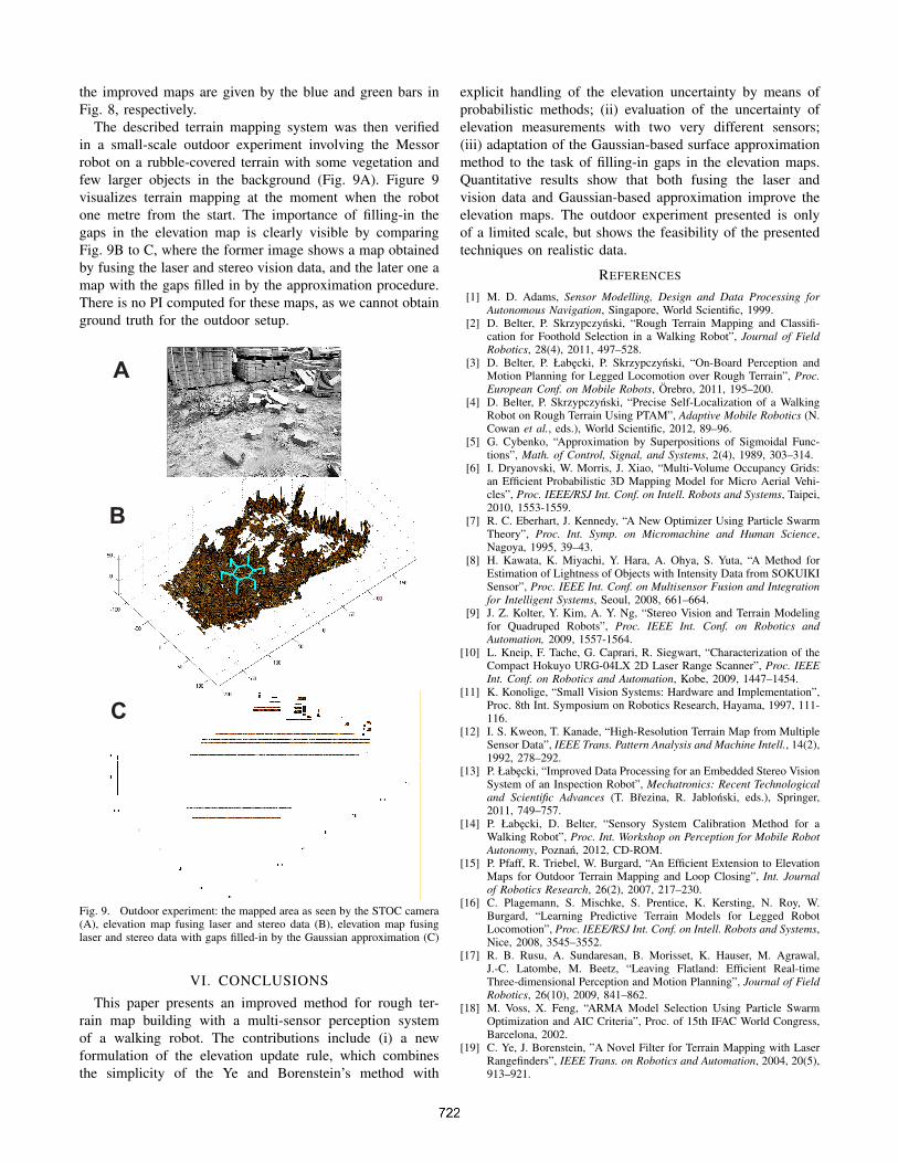
The described terrain mapping system was then verified
in a small-scale outdoor experiment involving the Messor
robot on a rubble-covered terrain with some vegetation and
few larger objects in the background (Fig. 9A). Figure 9
visualizes terrain mapping at the moment when the robot
one metre from the start. The importance of filling-in the
gaps in the elevation map is clearly visible by comparing
Fig. 9B to C, where the former image shows a map obtained
by fusing the laser and stereo vision data, and the later one a
map with the gaps filled in by the approximation procedure.
There is no PI computed for these maps, as we cannot obtain
ground truth for the outdoor setup.
A
B
C
Fig. 9. Outdoor experiment: the mapped area as seen by the STOC camera(A), elevation map fusing laser and stereo data (B), elevation map fusinglaser and stereo data with gaps filled-in by the Gaussian approximation (C)
VI. CONCLUSIONS
This paper presents an improved method for rough ter-
rain map building with a multi-sensor perception system
of a walking robot. The contributions include (i) a new
formulation of the elevation update rule, which combines
the simplicity of the Ye and Borenstein’s method with
explicit handling of the elevation uncertainty by means of
probabilistic methods; (ii) evaluation of the uncertainty of
elevation measurements with two very different sensors;
(iii) adaptation of the Gaussian-based surface approximation
method to the task of filling-in gaps in the elevation maps.
Quantitative results show that both fusing the laser and
vision data and Gaussian-based approximation improve the
elevation maps. The outdoor experiment presented is only
of a limited scale, but shows the feasibility of the presented
techniques on realistic data.
REFERENCES
[1] M. D. Adams, Sensor Modelling, Design and Data Processing for
Autonomous Navigation, Singapore, World Scientific, 1999.[2] D. Belter, P. Skrzypczynski, “Rough Terrain Mapping and Classifi-
cation for Foothold Selection in a Walking Robot”, Journal of Field
Robotics, 28(4), 2011, 497–528.[3] D. Belter, P. Łabecki, P. Skrzypczynski, “On-Board Perception and
Motion Planning for Legged Locomotion over Rough Terrain”, Proc.
European Conf. on Mobile Robots, Orebro, 2011, 195–200.[4] D. Belter, P. Skrzypczynski, “Precise Self-Localization of a Walking
Robot on Rough Terrain Using PTAM”, Adaptive Mobile Robotics (N.Cowan et al., eds.), World Scientific, 2012, 89–96.
[5] G. Cybenko, “Approximation by Superpositions of Sigmoidal Func-tions”, Math. of Control, Signal, and Systems, 2(4), 1989, 303–314.
[6] I. Dryanovski, W. Morris, J. Xiao, “Multi-Volume Occupancy Grids:an Efficient Probabilistic 3D Mapping Model for Micro Aerial Vehi-cles”, Proc. IEEE/RSJ Int. Conf. on Intell. Robots and Systems, Taipei,2010, 1553-1559.
[7] R. C. Eberhart, J. Kennedy, “A New Optimizer Using Particle SwarmTheory”, Proc. Int. Symp. on Micromachine and Human Science,Nagoya, 1995, 39–43.
[8] H. Kawata, K. Miyachi, Y. Hara, A. Ohya, S. Yuta, “A Method forEstimation of Lightness of Objects with Intensity Data from SOKUIKISensor”, Proc. IEEE Int. Conf. on Multisensor Fusion and Integration
for Intelligent Systems, Seoul, 2008, 661–664.[9] J. Z. Kolter, Y. Kim, A. Y. Ng, “Stereo Vision and Terrain Modeling
for Quadruped Robots”, Proc. IEEE Int. Conf. on Robotics and
Automation, 2009, 1557-1564.[10] L. Kneip, F. Tache, G. Caprari, R. Siegwart, “Characterization of the
Compact Hokuyo URG-04LX 2D Laser Range Scanner”, Proc. IEEE
Int. Conf. on Robotics and Automation, Kobe, 2009, 1447–1454.[11] K. Konolige, “Small Vision Systems: Hardware and Implementation”,
Proc. 8th Int. Symposium on Robotics Research, Hayama, 1997, 111-116.
[12] I. S. Kweon, T. Kanade, “High-Resolution Terrain Map from MultipleSensor Data”, IEEE Trans. Pattern Analysis and Machine Intell., 14(2),1992, 278–292.
[13] P. Łabecki, “Improved Data Processing for an Embedded Stereo VisionSystem of an Inspection Robot”, Mechatronics: Recent Technological
and Scientific Advances (T. Brezina, R. Jablonski, eds.), Springer,2011, 749–757.
[14] P. Łabecki, D. Belter, “Sensory System Calibration Method for aWalking Robot”, Proc. Int. Workshop on Perception for Mobile Robot
Autonomy, Poznan, 2012, CD-ROM.[15] P. Pfaff, R. Triebel, W. Burgard, “An Efficient Extension to Elevation
Maps for Outdoor Terrain Mapping and Loop Closing”, Int. Journal
of Robotics Research, 26(2), 2007, 217–230.[16] C. Plagemann, S. Mischke, S. Prentice, K. Kersting, N. Roy, W.
Burgard, “Learning Predictive Terrain Models for Legged RobotLocomotion”, Proc. IEEE/RSJ Int. Conf. on Intell. Robots and Systems,Nice, 2008, 3545–3552.
[17] R. B. Rusu, A. Sundaresan, B. Morisset, K. Hauser, M. Agrawal,J.-C. Latombe, M. Beetz, “Leaving Flatland: Efficient Real-timeThree-dimensional Perception and Motion Planning”, Journal of Field
Robotics, 26(10), 2009, 841–862.[18] M. Voss, X. Feng, “ARMA Model Selection Using Particle Swarm
Optimization and AIC Criteria”, Proc. of 15th IFAC World Congress,Barcelona, 2002.
[19] C. Ye, J. Borenstein, ”A Novel Filter for Terrain Mapping with LaserRangefinders”, IEEE Trans. on Robotics and Automation, 2004, 20(5),913–921.