estimating piacenzian sea surface temperature using an

U.S. Department of the InteriorU.S. Geological Survey

Scientific Investigations Report 2021–5051

Estimating Piacenzian Sea Surface Temperature Using an Alkenone-Calibrated Transfer Function

Cover. Planktic foraminifer specimens, arranged by species in numbered squares on a micropaleontological slide, provide assemblage data for quantitative analyses of sea surface conditions. Photograph by Christina Riesselman, U.S. Geological Survey.


By Harry J. Dowsett, Marci M. Robinson, and Kevin M. Foley

Scientific Investigations Report 2021–5051

U.S. Department of the InteriorU.S. Geological Survey

U.S. Geological Survey, Reston, Virginia: 2021

For more information on the USGS—the Federal source for science about the Earth, its natural and living resources, natural hazards, and the environment—visit https://www.usgs.gov or call 1–888–ASK–USGS.

For an overview of USGS information products, including maps, imagery, and publications, visit https://store.usgs.gov/.

Any use of trade, firm, or product names is for descriptive purposes only and does not imply endorsement by the U.S. Government.

Although this information product, for the most part, is in the public domain, it also may contain copyrighted materials as noted in the text. Permission to reproduce copyrighted items must be secured from the copyright owner.

Suggested citation:Dowsett, H.J., Robinson, M.M., and Foley, K.M., 2021, Estimating Piacenzian sea surface temperature using an alkenone-calibrated transfer function: U.S. Geological Survey Scientific Investigations Report 2021–5051, 17 p., https://doi.org/ 10.3133/ sir20215051.

Associated data for this publication:Dowsett, H.[J.], Robinson, M., and Foley, K., 2015, A global planktic foraminifer census data set for the Pliocene ocean: Scientific Data, v. 2, article 150076, 6 p., https://doi.org/ 10.1038/ sdata.2015.76.

Dowsett, H.J., Foley, K.M., Robinson, M.M., and Herbert, T.D., 2017, PRISM late Pliocene (Piacenzian) alkenone-derived SST data: U.S. Geological Survey data release, https://doi.org/ 10.5066/ F7959G1S.

Robinson, M.M., Foley, K., Dowsett, H.J., and Spivey, W., 2019, A global planktic foraminifer census data set for the Pliocene ocean, addendum: National Oceanic and Atmospheric Administration, National Centers for Environmental Information [formerly National Climatic Data Center] website, https: //www.ncdc .noaa.gov/ paleo/ study/ 27310.

ISSN 2328-0328 (online)

https://doi.org/10.3133/sir20215051

https://doi.org/10.1038/sdata.2015.76

https://doi.org/10.5066/F7959G1S

https://www.ncdc.noaa.gov/paleo/study/27310

iii

Acknowledgments

The research described in this report used samples provided by the International Ocean Discovery Program (IODP), the Ocean Drilling Program (ODP), and the Deep Sea Drilling Project (DSDP).

Funding for this research was provided by the U.S. Geological Survey (USGS) Land Change Science Program through the Geological Investigations of the Neogene Project. Tim Herbert of Brown University collaborated on analysis and discussion of alkenone data. Peer reviews by Thomas Cronin and Summer Praetorius of the USGS were helpful.

v

ContentsAcknowledgments ........................................................................................................................................iiiAbstract ...........................................................................................................................................................1Background and Introduction ......................................................................................................................1Materials and Methods.................................................................................................................................2

Chronology .............................................................................................................................................2Faunal Census Data ..............................................................................................................................2Sea Surface Temperature Data ..........................................................................................................2Quantitative Analysis............................................................................................................................2

Results .............................................................................................................................................................7Assemblage Analysis ...........................................................................................................................7Paleotemperature Equation ..............................................................................................................11

Discussion .....................................................................................................................................................11Use of New Transfer Function ..........................................................................................................11North Atlantic Sea Surface Temperature .......................................................................................11

Summary and Conclusions .........................................................................................................................13References Cited..........................................................................................................................................13Appendix 1. Species List .........................................................................................................................16

Figures

1. Graph showing the PRISM3 interval (also known as the mid-Piacenzian Warm Period [mPWP]) in relation to paleomagnetic reversal stratigraphy, planktonic foraminiferal zones, and the long-term climate evolution of the Pliocene Epoch .............3

2. Graph of results of factor analysis of Piacenzian planktonic foraminiferal assemblages showing sample loadings on Factor 1 and Factor 2 .......................................8

3. Graphic representation of the assemblage description matrix showing how foraminiferal species score on five factors and percentage of information explained ........................................................................................................................................9

4. Dendrogram and map showing results of cluster analysis of planktonic foraminiferal assemblages from 31 sites and geographic distribution of cluster groups .............................................................................................................................10

5. Map showing PRISM3 mean sea surface temperatures (SST) for 31 sites in the North Atlantic Ocean .................................................................................................................12

Tables

1. Site locations, alkenone-based sea surface temperature estimates, number of samples, and faunal abundance data used in this study .......................................................4

2. Factor loadings explaining the relative contribution of the five factors to the faunal assemblage at each site .................................................................................................6

3. Factor scores for the five-factor model indicating influence of taxa from 31 sites on factors .........................................................................................................................7

vi

Conversion FactorsTemperature in degrees Celsius (°C) may be converted to degrees Fahrenheit (°F) as follows:

°F = (1.8 × °C) + 32.

Temperature in degrees Fahrenheit (°F) may be converted to degrees Celsius (°C) as follows: °C = (°F – 32) / 1.8.

Abbreviations~ approximately

≤ less than or equal to

± plus or minus

δ18O a measure of the ratio of stable isotopes oxygen-18 (18O) and oxygen-16 (16O)

CLIMAP Climate: Long range Investigation, Mapping, and Prediction

DSDP Deep Sea Drilling Project

IODP International Ocean Discovery Program

kyr kilo-years (thousand years)

Ma mega-annum (million years ago)

MIS Marine Isotope Stage

mPWP mid-Piacenzian Warm Period

ODP Ocean Drilling Program

PL3 planktonic foraminiferal zone 3 for the Pliocene

PRISM Pliocene Research, Interpretation and Synoptic Mapping

SST sea surface temperature

U 37 K ′ temperature index derived from long-chain unsaturated ketones (C37 alkenones) produced by Emiliania huxleyi and found in sediments

UPGMA Unweighted Pair Group Method with Arithmetic Mean

USGS U.S. Geological Survey


By Harry J. Dowsett, Marci M. Robinson, and Kevin M. Foley

AbstractStationarity of environmental preferences is a primary

assumption required for any paleoenvironmental reconstruc-tion using fossil materials based upon calibration to modern organisms. Confidence in this assumption decreases the further back in time one goes, and the validity of the assumption that species temperature tolerances have not changed over time has been challenged in Pliocene studies. We use paired U 37 K ′ (unsaturated ketones with 37 carbon atoms) sea surface tem-perature (SST) and faunal assemblage data to directly calibrate North Atlantic Piacenzian planktonic foraminifer assemblages to Piacenzian alkenone paleotemperature estimates to provide an alternative paleoceanographic reconstruction approach that does not rely on stationarity. In doing so, we extend Pliocene SST estimates to sites where only quantitative faunal assem-blage data were previously available and improve the spatial resolution of the North Atlantic SST reconstruction.

Background and IntroductionForaminiferal census data have been routinely used to

quantitatively estimate paleoceanographic temperature since the 1970s with the introduction of a method for deriving fac-tor analytic transfer functions (Imbrie and Kipp, 1971). The Imbrie-Kipp method relates modern species abundance data to physical oceanographic parameters to derive equations that are then used on fossil assemblages to make quantitative estimates of paleoenvironments. This technique was used extensively in (1) the reconstruction of the Last Glacial Maximum by members of CLIMAP (Climate: Long range Investigation, Mapping, and Prediction) (Cline and Hays, 1976) and (2) the later reconstruction of the Last Interglacial (CLIMAP Project Members, 1984). The Imbrie-Kipp method and other methods like the Modern Analog Technique, in which fossil assemblages are assigned the sea surface temperature (SST) of the most analogous assemblage within a modern dataset (Hutson, 1980), and methods using artificial neural networks to discover patterns within data (for example, Malmgren and Nordlund, 1997; Malmgren and others, 2001) all rely on the basic assumption that modern foraminiferal faunas

can be used as analogs to interpret Quaternary assemblages. Extensions of these methods to deeper time settings like the Piacenzian Age (3.60 to 2.58 million years ago [Ma]) of the Pliocene Epoch require additional assumptions to address extinction and evolution of species since that time (Keigwin, 1976; Thunell, 1979; Dowsett and Poore, 1990; Sabaa and others, 2004) and require the ability to correlate time series data among many sites across all ocean basins (Dowsett and Robinson, 2006). These two challenges—assumptions regard-ing species tolerances and uncertain chronologic correlation—insert uncertainty into pre-Quaternary paleoenvironmental reconstructions.

Paramount to all paleoenvironmental reconstructions, whether paleontological or geochemical in nature, is the con-cept of stationarity, the assumption that the relations among variables have not changed over time. Faunal assemblage-based reconstructions depend on the assumption of stationarity of environmental tolerances or preferences of the extant spe-cies that are in the fossil assemblage. In addition, now extinct species must be assigned the tolerances of extant taxa on the basis of ancestor-descendent relationships and (or) similar spatial distributions. For example, the U.S. Geological Survey (USGS) reconstructions of the North Atlantic paleoclimate through the Pliocene Research, Interpretation and Synoptic Mapping (PRISM) studies are based in part on transfer func-tions that incorporated modern species absent from Pliocene assemblages as well as Pliocene species now extinct (Dowsett and Poore, 1990).

The lack of evidence in support of the constancy of environmental tolerance of species remains a stumbling block for paleoenvironmental reconstruction. A second obstacle is the inability to establish high-confidence deep-time chronol-ogy and correlation among multiple deep-sea sites where the sediment accumulation rate is relatively low and bioturbation is common. Although a plethora of Piacenzian planktonic fora-miniferal census data exist, the temporal density of samples within and between cores is highly variable, thus hindering the accurate correlation and calibration of coeval samples from different localities on the basis of current age models (Dowsett and others, 2019).

In this report, these concerns are addressed by presenting an alternative approach to paleotemperature estimation that uses foraminiferal census data calibrated directly to Piacenzian temperatures derived from alkenone paleothermometry,

2 Estimating Piacenzian Sea Surface Temperature Using an Alkenone-Calibrated Transfer Function

thereby eliminating the need for stationarity in environ-mental preferences beyond the time interval covered by the study. We averaged both faunal abundance data and alke-none data, within a defined stratigraphic interval (dated at 3.264–3.025 Ma), to accommodate the uneven temporal distribution of samples within and between core sites. This averaging effectively passed the data through a low-pass filter, thereby eliminating the possibility of estimating high-frequency variability. We accepted this limitation in order to establish general warming and cooling trends in Pliocene time series.

Materials and Methods

Chronology

In our study, we focused on a period of warm and stable climate (relative to high-amplitude Pleistocene glacial-interglacial cycles) positioned within the Piacenzian Stage known as the PRISM3 interval or mid-Piacenzian Warm Period (mPWP) (fig. 1). It extends from the Marine Isotope Stage (MIS) M2/M1 boundary (3.264 Ma) to the G21/G20 boundary (3.025 Ma) in the middle part of the Gauss normal polarity Chron (Dowsett and others, 2010, 2016). As defined, the interval lasted about 240,000 years (~240 kyr) and ranged from C2An2r (Mammoth reversed polarity) to near the bottom of C2An1 (just above Kaena reversed polarity). This interval correlates in part with planktonic foraminiferal zones PL3 (Sphaeroidinellopsis seminulina Highest Occurrence Zone), PL4 (Dentoglobigerina altispira Highest Occurrence Zone), and PL5 (Globorotalia miocenica Highest Occurrence Zone). Within the bounding positive δ18O excursions that mark gla-cial stages M2 and G20, and excepting glacial stage KM2 at ~3.1 Ma, benthic foraminiferal oxygen isotope values in this interval are equal to or isotopically lighter than those mea-sured today.

Faunal Census Data

Planktonic foraminiferal abundance data were selected from the PRISM3 interval of 31 sites in the North Atlantic Ocean (Dowsett and others, 2015; Robinson and others, 2019); the sites were drilled by the Deep Sea Drilling Project (DSDP), Ocean Drilling Program (ODP), and International Ocean Discovery Program (IODP). The temporal distribution of samples within this interval at each site is highly vari-able, and establishing synchronous samples from the differ-ent localities, based upon existing age models, is unrealistic. Therefore, samples collected from within the stratigraphic interval dated at 3.264–3.025 Ma at each site were averaged

to obtain mean abundances. Species with mean abundances ≤1 percent were deleted. The resulting dataset contains percent mean abundance data for 23 counting categories at each of the 31 North Atlantic sites (table 1). Taxonomic concepts are those of Parker (1962, 1967), Blow (1969), and Dowsett and Robinson (2007). A species list is provided in appendix 1.

Sea Surface Temperature Data

The U 37 K ′ (unsaturated ketones with 37 carbon atoms) unsaturation index was used to obtain SST estimates from the PRISM3 interval of 17 sites in the North Atlantic (table 1). Temperature estimates using this technique generally have an analytical error of ±0.1 °C (Herbert and others, 1995; Lawrence and others, 2007). All temperature estimates were calibrated by using the method of Müller and others (1998) and have a calibration uncertainty of ±1.38 °C (Lawrence and others, 2007). Alkenone data used have been previously published (Robinson and others, 2008; Lawrence and others, 2009; Herbert and others, 2010; Lawrence and others, 2010; Naafs and others, 2010; Khélifi and others, 2012; Badger and others, 2013; Dowsett and others, 2017, 2019). As with the faunal data, a single SST estimate was obtained for the PRISM3 stratigraphic interval, which represents the mean of individual U 37 K ′ estimates for samples dated between 3.264 and 3.025 Ma at each site (table 1).

Quantitative Analysis

Q-mode factor analysis (Klovan and Imbrie, 1971) was used to reduce the dimensionality of the Pliocene faunal data. The process is summarized by the following equation:

Up = BpFp + E (1)

where Up represents the normalized Pliocene foraminiferal census; Bp represents the varimax factor loadings matrix providing the contribution of each factor to the assemblage; Fp represents the factor description (scores) matrix, which describes the composition of the factors; and E represents an error matrix.

Sample communality (h2) is provided to assess how well the factor model explains the data in each sample. Communality is expressed as the sum of the squares of the factor loadings (f), for factors 1 through n:

(2)

A sample communality of 1 indicates a perfect fit of model and data, with E = 0.

h fn n2

12

Materials and Methods 3

2.0

3.0

4.0

4.8

4.6

4.4

4.2

3.8

3.6

3.4

3.2

2.8

2.6

2.4

2.2

5.0

5.24.00 3.50 3.00 2.50

Mat

uyam

aGa

uss

Gilb

ert

K

M

C

N

S

T

Chro

n

Plio

cene

Plei

stoc

ene

Epoc

h

Pola

rity

M2

KM2mPWP

Age

(Ma)

KM5

M1

K1

KM3

KM1

G21

KM2

Gela

sian

Zanc

lean

Age

Piac

enzia

n

PL2

PL1

PL3

PL5

PL6

Zone

PL4

G20

4.25 3.75 3.25 2.75LR04 stack of benthic 18O records (‰)

PRISM3 INTERVAL

Figure 1. Graph showing the PRISM3 interval (also known as the mid-Piacenzian Warm Period [mPWP]) in relation to paleomagnetic reversal stratigraphy, planktonic foraminiferal zones, and the long-term climate evolution of the Pliocene Epoch. The LR04 benthic oxygen isotope stack and time scale are from Lisiecki and Raymo (2005); δ18O values are in parts per thousand (‰). The vertical dashed line shows the δ18O value for the present-day ocean. The PRISM3 stratigraphic interval (dated at 3.264–3.025 million years ago [Ma]) is shown relative to Marine Isotope Stages M2, M1, KM5, KM3, KM2, KM1, K1, G21, and G20 from Lisiecki and Raymo (2005). The subchrons in the polarity column of the paleomagnetic data are from Ogg and others (2016): T, Thvera; S, Sidufjall; N, Nunivak; C, Cochiti; M, Mammoth; K, Kaena. Black segments indicate normal polarity, and white segments indicate reversed polarity. The planktonic foraminiferal zones PL1 to PL6 for the Pliocene are from Berggren (1973).


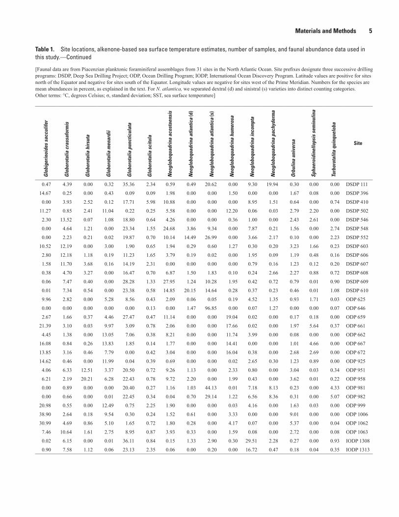
Table 1. Site locations, alkenone-based sea surface temperature estimates, number of samples, and faunal abundance data used in this study.

[Faunal data are from Piacenzian planktonic foraminiferal assemblages from 31 sites in the North Atlantic Ocean. Site prefixes designate three successive drilling programs: DSDP, Deep Sea Drilling Project; ODP, Ocean Drilling Program; IODP, International Ocean Discovery Program. Latitude values are positive for sites north of the Equator and negative for sites south of the Equator. Longitude values are negative for sites west of the Prime Meridian. Numbers for the species are mean abundances in percent, as explained in the text. For N. atlantica, we separated dextral (d) and sinistral (s) varieties into distinct counting categories. Other terms: °C, degrees Celsius; σ, standard deviation; SST, sea surface temperature]

SiteLatitude

(°)Longitude

(°)Alkenone

SST (°C) (σ)

Number of

alkenone samples

Number of faunal samples

Den

togl

obig

erin

a al

tispi

ra

Glo

bige

rina

bul

loid

es

Glo

bige

rina

falc

onen

sis

Glo

bige

rina

woo

di

Glo

bige

rine

lla a

equi

late

ralis

Glo

bige

rini

ta g

lutin

ata

Glo

bige

rino

ides

obl

iquu

s

Glo

bige

rino

ides

rube

r

Glo

bige

rino

ides

sac

culif

er

Glo

boro

talia

cra

ssaf

orm

is

Glo

boro

talia

hir

suta

Glo

boro

talia

men

ardi

i

Glo

boro

talia

pun

ctic

ulat

a

Glo

boro

talia

sci

tula

Neo

glob

oqua

drin

a ac

osta

ensi

s

Neo

glob

oqua

drin

a at

lant

ica

(d)

Neo

glob

oqua

drin

a at

lant

ica

(s)

Neo

glob

oqua

drin

a hu

mer

osa

Neo

glob

oqua

drin

a in

com

pta

Neo

glob

oqua

drin

a pa

chyd

erm

a

Orb

ulin

a un

iver

sa

Spha

eroi

dine

llops

is s

emin

ulin

a

Turb

orot

alita

qui

nque

loba

Site

DSDP 111 50.43 −46.37 — — 2 0.00 0.78 0.49 0.64 0.00 3.33 0.51 0.15 0.47 4.39 0.00 0.32 35.36 2.34 0.59 0.49 20.62 0.00 9.30 19.94 0.30 0.00 0.00 DSDP 111

DSDP 396 22.48 −43.52 — — 4 0.00 0.65 0.08 3.33 1.96 2.65 39.04 31.53 14.67 0.25 0.00 0.43 0.09 0.09 1.98 0.00 0.00 1.50 0.00 0.00 1.67 0.08 0.00 DSDP 396

DSDP 410 45.51 −29.48 — — 3 0.00 20.38 10.76 7.62 0.37 7.90 0.00 0.00 0.00 3.93 2.52 0.12 17.71 5.98 10.88 0.00 0.00 0.00 8.95 1.51 0.64 0.00 0.74 DSDP 410

DSDP 502 11.49 −79.38 — — 23 4.88 7.48 0.67 10.55 1.12 8.19 5.91 12.32 11.27 0.85 2.41 11.04 0.22 0.25 5.58 0.00 0.00 12.20 0.06 0.03 2.79 2.20 0.00 DSDP 502

DSDP 546 33.78 −9.56 — — 5 0.20 15.27 2.53 8.84 1.28 12.69 3.23 8.87 2.30 13.52 0.07 1.08 18.80 0.64 4.26 0.00 0.00 0.36 1.00 0.00 2.43 2.61 0.00 DSDP 546

DSDP 548 48.92 −12.16 — — 23 0.00 5.04 2.86 3.05 0.67 7.38 0.00 0.00 0.00 4.64 1.21 0.00 23.34 1.55 24.68 3.86 9.34 0.00 7.87 0.21 1.56 0.00 2.74 DSDP 548

DSDP 552 56.04 −23.23 17.43 (1.52) 12 13 0.00 6.54 1.07 1.02 0.23 8.35 0.00 0.00 0.00 2.23 0.21 0.02 19.87 0.70 10.14 14.49 26.99 0.00 3.66 2.17 0.10 0.00 2.23 DSDP 552

DSDP 603 35.50 −70.03 22.41 (0.65) 11 9 2.99 3.76 10.75 5.68 0.77 13.53 9.60 14.95 10.52 12.19 0.00 3.00 1.90 0.65 1.94 0.29 0.60 1.27 0.30 0.20 3.23 1.66 0.23 DSDP 603

DSDP 606 37.34 −35.50 21.64 (1.02) 24 23 0.97 10.80 15.79 12.42 2.44 10.52 4.43 5.54 2.80 12.18 1.18 0.19 11.23 1.65 3.79 0.19 0.02 0.00 1.95 0.09 1.19 0.48 0.16 DSDP 606

DSDP 607 41.00 −32.96 21.04 (0.62) 12 12 0.47 25.06 2.16 10.86 3.62 14.96 1.62 5.10 1.58 11.70 3.68 0.16 14.19 2.31 0.00 0.00 0.00 0.00 0.79 0.16 1.23 0.12 0.20 DSDP 607

DSDP 608 42.84 −23.09 — — 11 0.07 13.26 16.56 15.61 0.00 8.05 1.37 2.50 0.38 4.70 3.27 0.00 16.47 0.70 6.87 1.50 1.83 0.10 0.24 2.66 2.27 0.88 0.72 DSDP 608

DSDP 609 49.88 −24.24 17.98 (1.25) 23 23 0.06 5.60 1.13 1.75 0.17 9.29 0.03 0.17 0.06 7.47 0.40 0.00 28.28 1.33 27.95 1.24 10.28 1.95 0.42 0.72 0.79 0.01 0.90 DSDP 609

DSDP 610 53.22 −18.89 — — 23 0.00 5.09 1.00 1.16 0.47 8.31 0.00 0.04 0.01 7.34 0.54 0.00 23.38 0.58 14.85 20.15 14.64 0.28 0.37 0.23 0.46 0.01 1.08 DSDP 610

ODP 625 28.83 −87.16 21.17 (0.35) 13 13 7.21 3.85 3.69 3.88 0.24 17.66 11.90 13.59 9.96 2.82 0.00 5.28 8.56 0.43 2.09 0.06 0.05 0.19 4.52 1.35 0.93 1.71 0.03 ODP 625

ODP 646 58.21 −48.37 — — 5 0.00 0.13 0.00 0.00 0.00 0.00 0.00 0.00 0.00 0.00 0.00 0.00 0.00 0.13 0.00 1.47 96.85 0.00 0.07 1.27 0.00 0.00 0.07 ODP 646

ODP 659 18.08 −21.03 — — 16 3.12 8.83 0.16 2.26 0.00 6.86 4.56 6.53 2.67 1.66 0.37 4.46 27.47 0.47 11.14 0.00 0.00 19.04 0.02 0.00 0.17 0.18 0.00 ODP 659

ODP 661 9.45 −19.39 — — 22 8.00 5.70 0.01 3.01 0.77 2.45 7.04 6.92 21.39 3.10 0.03 9.97 3.09 0.78 2.06 0.00 0.00 17.66 0.02 0.00 1.97 5.64 0.37 ODP 661

ODP 662 −1.39 −11.74 27.25 (0.15) 23 19 15.35 4.07 1.38 3.45 0.31 13.20 5.07 6.83 4.45 1.38 0.00 13.05 7.06 0.38 8.21 0.00 0.00 11.74 3.99 0.00 0.08 0.00 0.00 ODP 662

ODP 667 4.57 −21.91 — — 11 15.70 3.67 0.84 1.47 1.14 3.60 12.71 6.04 16.08 0.84 0.26 13.83 1.85 0.14 1.77 0.00 0.00 14.41 0.00 0.00 1.01 4.66 0.00 ODP 667

ODP 672 15.54 −58.64 — — 5 12.92 1.25 0.00 3.35 0.35 6.13 12.13 13.37 13.85 3.16 0.46 7.79 0.00 0.42 3.04 0.00 0.00 16.04 0.38 0.00 2.68 2.69 0.00 ODP 672

ODP 925 4.20 −43.49 28.57 (0.54) 28 22 14.57 1.20 0.68 4.39 1.14 11.41 14.58 18.76 14.62 0.46 0.00 11.99 0.04 0.39 0.69 0.00 0.00 0.02 2.65 0.30 1.23 0.89 0.00 ODP 925

ODP 951 32.03 −24.87 24.24 (0.97) 21 21 2.07 9.41 3.64 3.19 0.58 4.47 4.95 7.28 4.06 6.33 12.51 3.37 20.50 0.72 9.26 1.13 0.00 2.33 0.80 0.00 3.04 0.03 0.34 ODP 951

ODP 958 24.00 −20.00 24.62 (0.88) 25 24 1.47 6.48 1.61 1.31 0.84 1.70 4.17 6.13 6.21 2.19 20.21 6.28 22.43 0.78 9.72 2.20 0.00 1.99 0.43 0.00 3.62 0.01 0.22 ODP 958

ODP 981 55.48 −14.65 — — 31 0.00 1.55 2.12 0.13 0.00 8.45 0.00 0.01 0.00 0.89 0.00 0.00 20.40 0.27 1.16 1.03 44.13 0.01 7.18 8.13 0.23 0.00 4.33 ODP 981

ODP 982 57.52 −15.87 17.64 (1.33) 36 48 0.00 10.09 1.15 0.25 0.49 13.16 0.00 0.00 0.00 0.66 0.00 0.01 22.45 0.34 0.04 0.70 29.14 1.22 6.56 8.36 0.31 0.00 5.07 ODP 982

ODP 999 12.74 −78.74 28.00 (0.11) 2 18 4.69 8.89 1.84 8.74 0.20 10.45 8.11 12.32 20.98 0.55 0.00 12.49 0.75 2.25 1.90 0.00 0.00 0.03 4.16 0.00 1.63 0.03 0.00 ODP 999

ODP 1006 24.40 −79.46 28.29 (0.39) 6 24 2.62 1.04 1.22 0.68 2.68 0.65 8.05 16.81 38.90 2.64 0.18 9.54 0.30 0.24 1.52 0.61 0.00 3.33 0.00 0.00 9.01 0.00 0.00 ODP 1006

ODP 1062 33.69 −57.62 23.57 (0.61) 28 23 2.95 2.14 3.46 5.70 0.98 2.73 8.70 17.60 30.99 4.69 0.86 5.10 1.65 0.72 1.80 0.28 0.00 4.17 0.07 0.00 5.37 0.00 0.04 ODP 1062

ODP 1063 33.69 −57.62 22.67 (0.54) 15 23 2.06 7.05 13.49 7.35 0.55 10.83 7.62 10.02 7.46 10.64 1.61 2.75 8.95 0.87 3.93 0.33 0.00 1.59 0.08 0.00 2.72 0.00 0.08 ODP 1063

IODP 1308 49.88 −24.24 18.13 (0.95) 57 27 0.26 4.98 2.56 1.20 0.76 9.33 0.02 0.09 0.02 6.15 0.00 0.01 36.11 0.84 0.15 1.33 2.90 0.30 29.51 2.28 0.27 0.00 0.93 IODP 1308

IODP 1313 41.00 −32.96 21.06 (0.79) 28 18 1.78 8.15 7.76 3.92 1.08 20.31 1.59 2.23 0.90 7.58 1.12 0.06 23.13 2.35 0.06 0.00 0.20 0.00 16.72 0.47 0.18 0.04 0.35 IODP 1313

Materials and Methods 5

Table 1. Site locations, alkenone-based sea surface temperature estimates, number of samples, and faunal abundance data used in this study.


SiteLatitude

(°)Longitude

(°)Alkenone

SST (°C) (σ)

Number of

alkenone samples

Number of faunal samples

Den

togl

obig

erin

a al

tispi

ra

Glo

bige

rina

bul

loid

es

Glo

bige

rina

falc

onen

sis

Glo

bige

rina

woo

di

Glo

bige

rine

lla a

equi

late

ralis

Glo

bige

rini

ta g

lutin

ata

Glo

bige

rino

ides

obl

iquu

s

Glo

bige

rino

ides

rube

r

Glo

bige

rino

ides

sac

culif

er

Glo

boro

talia

cra

ssaf

orm

is

Glo

boro

talia

hir

suta

Glo

boro

talia

men

ardi

i

Glo

boro

talia

pun

ctic

ulat

a

Glo

boro

talia

sci

tula

Neo

glob

oqua

drin

a ac

osta

ensi

s

Neo

glob

oqua

drin

a at

lant

ica

(d)

Neo

glob

oqua

drin

a at

lant

ica

(s)

Neo

glob

oqua

drin

a hu

mer

osa

Neo

glob

oqua

drin

a in

com

pta

Neo

glob

oqua

drin

a pa

chyd

erm

a

Orb

ulin

a un

iver

sa

Spha

eroi

dine

llops

is s

emin

ulin

a

Turb

orot

alita

qui

nque

loba

Site

DSDP 111 50.43 −46.37 — — 2 0.00 0.78 0.49 0.64 0.00 3.33 0.51 0.15 0.47 4.39 0.00 0.32 35.36 2.34 0.59 0.49 20.62 0.00 9.30 19.94 0.30 0.00 0.00 DSDP 111

DSDP 396 22.48 −43.52 — — 4 0.00 0.65 0.08 3.33 1.96 2.65 39.04 31.53 14.67 0.25 0.00 0.43 0.09 0.09 1.98 0.00 0.00 1.50 0.00 0.00 1.67 0.08 0.00 DSDP 396

DSDP 410 45.51 −29.48 — — 3 0.00 20.38 10.76 7.62 0.37 7.90 0.00 0.00 0.00 3.93 2.52 0.12 17.71 5.98 10.88 0.00 0.00 0.00 8.95 1.51 0.64 0.00 0.74 DSDP 410

DSDP 502 11.49 −79.38 — — 23 4.88 7.48 0.67 10.55 1.12 8.19 5.91 12.32 11.27 0.85 2.41 11.04 0.22 0.25 5.58 0.00 0.00 12.20 0.06 0.03 2.79 2.20 0.00 DSDP 502

DSDP 546 33.78 −9.56 — — 5 0.20 15.27 2.53 8.84 1.28 12.69 3.23 8.87 2.30 13.52 0.07 1.08 18.80 0.64 4.26 0.00 0.00 0.36 1.00 0.00 2.43 2.61 0.00 DSDP 546

DSDP 548 48.92 −12.16 — — 23 0.00 5.04 2.86 3.05 0.67 7.38 0.00 0.00 0.00 4.64 1.21 0.00 23.34 1.55 24.68 3.86 9.34 0.00 7.87 0.21 1.56 0.00 2.74 DSDP 548

DSDP 552 56.04 −23.23 17.43 (1.52) 12 13 0.00 6.54 1.07 1.02 0.23 8.35 0.00 0.00 0.00 2.23 0.21 0.02 19.87 0.70 10.14 14.49 26.99 0.00 3.66 2.17 0.10 0.00 2.23 DSDP 552

DSDP 603 35.50 −70.03 22.41 (0.65) 11 9 2.99 3.76 10.75 5.68 0.77 13.53 9.60 14.95 10.52 12.19 0.00 3.00 1.90 0.65 1.94 0.29 0.60 1.27 0.30 0.20 3.23 1.66 0.23 DSDP 603

DSDP 606 37.34 −35.50 21.64 (1.02) 24 23 0.97 10.80 15.79 12.42 2.44 10.52 4.43 5.54 2.80 12.18 1.18 0.19 11.23 1.65 3.79 0.19 0.02 0.00 1.95 0.09 1.19 0.48 0.16 DSDP 606

DSDP 607 41.00 −32.96 21.04 (0.62) 12 12 0.47 25.06 2.16 10.86 3.62 14.96 1.62 5.10 1.58 11.70 3.68 0.16 14.19 2.31 0.00 0.00 0.00 0.00 0.79 0.16 1.23 0.12 0.20 DSDP 607

DSDP 608 42.84 −23.09 — — 11 0.07 13.26 16.56 15.61 0.00 8.05 1.37 2.50 0.38 4.70 3.27 0.00 16.47 0.70 6.87 1.50 1.83 0.10 0.24 2.66 2.27 0.88 0.72 DSDP 608

DSDP 609 49.88 −24.24 17.98 (1.25) 23 23 0.06 5.60 1.13 1.75 0.17 9.29 0.03 0.17 0.06 7.47 0.40 0.00 28.28 1.33 27.95 1.24 10.28 1.95 0.42 0.72 0.79 0.01 0.90 DSDP 609

DSDP 610 53.22 −18.89 — — 23 0.00 5.09 1.00 1.16 0.47 8.31 0.00 0.04 0.01 7.34 0.54 0.00 23.38 0.58 14.85 20.15 14.64 0.28 0.37 0.23 0.46 0.01 1.08 DSDP 610

ODP 625 28.83 −87.16 21.17 (0.35) 13 13 7.21 3.85 3.69 3.88 0.24 17.66 11.90 13.59 9.96 2.82 0.00 5.28 8.56 0.43 2.09 0.06 0.05 0.19 4.52 1.35 0.93 1.71 0.03 ODP 625

ODP 646 58.21 −48.37 — — 5 0.00 0.13 0.00 0.00 0.00 0.00 0.00 0.00 0.00 0.00 0.00 0.00 0.00 0.13 0.00 1.47 96.85 0.00 0.07 1.27 0.00 0.00 0.07 ODP 646

ODP 659 18.08 −21.03 — — 16 3.12 8.83 0.16 2.26 0.00 6.86 4.56 6.53 2.67 1.66 0.37 4.46 27.47 0.47 11.14 0.00 0.00 19.04 0.02 0.00 0.17 0.18 0.00 ODP 659

ODP 661 9.45 −19.39 — — 22 8.00 5.70 0.01 3.01 0.77 2.45 7.04 6.92 21.39 3.10 0.03 9.97 3.09 0.78 2.06 0.00 0.00 17.66 0.02 0.00 1.97 5.64 0.37 ODP 661

ODP 662 −1.39 −11.74 27.25 (0.15) 23 19 15.35 4.07 1.38 3.45 0.31 13.20 5.07 6.83 4.45 1.38 0.00 13.05 7.06 0.38 8.21 0.00 0.00 11.74 3.99 0.00 0.08 0.00 0.00 ODP 662

ODP 667 4.57 −21.91 — — 11 15.70 3.67 0.84 1.47 1.14 3.60 12.71 6.04 16.08 0.84 0.26 13.83 1.85 0.14 1.77 0.00 0.00 14.41 0.00 0.00 1.01 4.66 0.00 ODP 667

ODP 672 15.54 −58.64 — — 5 12.92 1.25 0.00 3.35 0.35 6.13 12.13 13.37 13.85 3.16 0.46 7.79 0.00 0.42 3.04 0.00 0.00 16.04 0.38 0.00 2.68 2.69 0.00 ODP 672

ODP 925 4.20 −43.49 28.57 (0.54) 28 22 14.57 1.20 0.68 4.39 1.14 11.41 14.58 18.76 14.62 0.46 0.00 11.99 0.04 0.39 0.69 0.00 0.00 0.02 2.65 0.30 1.23 0.89 0.00 ODP 925

ODP 951 32.03 −24.87 24.24 (0.97) 21 21 2.07 9.41 3.64 3.19 0.58 4.47 4.95 7.28 4.06 6.33 12.51 3.37 20.50 0.72 9.26 1.13 0.00 2.33 0.80 0.00 3.04 0.03 0.34 ODP 951

ODP 958 24.00 −20.00 24.62 (0.88) 25 24 1.47 6.48 1.61 1.31 0.84 1.70 4.17 6.13 6.21 2.19 20.21 6.28 22.43 0.78 9.72 2.20 0.00 1.99 0.43 0.00 3.62 0.01 0.22 ODP 958

ODP 981 55.48 −14.65 — — 31 0.00 1.55 2.12 0.13 0.00 8.45 0.00 0.01 0.00 0.89 0.00 0.00 20.40 0.27 1.16 1.03 44.13 0.01 7.18 8.13 0.23 0.00 4.33 ODP 981

ODP 982 57.52 −15.87 17.64 (1.33) 36 48 0.00 10.09 1.15 0.25 0.49 13.16 0.00 0.00 0.00 0.66 0.00 0.01 22.45 0.34 0.04 0.70 29.14 1.22 6.56 8.36 0.31 0.00 5.07 ODP 982

ODP 999 12.74 −78.74 28.00 (0.11) 2 18 4.69 8.89 1.84 8.74 0.20 10.45 8.11 12.32 20.98 0.55 0.00 12.49 0.75 2.25 1.90 0.00 0.00 0.03 4.16 0.00 1.63 0.03 0.00 ODP 999

ODP 1006 24.40 −79.46 28.29 (0.39) 6 24 2.62 1.04 1.22 0.68 2.68 0.65 8.05 16.81 38.90 2.64 0.18 9.54 0.30 0.24 1.52 0.61 0.00 3.33 0.00 0.00 9.01 0.00 0.00 ODP 1006

ODP 1062 33.69 −57.62 23.57 (0.61) 28 23 2.95 2.14 3.46 5.70 0.98 2.73 8.70 17.60 30.99 4.69 0.86 5.10 1.65 0.72 1.80 0.28 0.00 4.17 0.07 0.00 5.37 0.00 0.04 ODP 1062

ODP 1063 33.69 −57.62 22.67 (0.54) 15 23 2.06 7.05 13.49 7.35 0.55 10.83 7.62 10.02 7.46 10.64 1.61 2.75 8.95 0.87 3.93 0.33 0.00 1.59 0.08 0.00 2.72 0.00 0.08 ODP 1063

IODP 1308 49.88 −24.24 18.13 (0.95) 57 27 0.26 4.98 2.56 1.20 0.76 9.33 0.02 0.09 0.02 6.15 0.00 0.01 36.11 0.84 0.15 1.33 2.90 0.30 29.51 2.28 0.27 0.00 0.93 IODP 1308

IODP 1313 41.00 −32.96 21.06 (0.79) 28 18 1.78 8.15 7.76 3.92 1.08 20.31 1.59 2.23 0.90 7.58 1.12 0.06 23.13 2.35 0.06 0.00 0.20 0.00 16.72 0.47 0.18 0.04 0.35 IODP 1313

Table 1. Site locations, alkenone-based sea surface temperature estimates, number of samples, and faunal abundance data used in this study.—Continued



Table 2. Factor loadings explaining the relative contribution of the five factors to the faunal assemblage at each site.

[Sites are identified in table 1. NA, not applicable]

Site Factor 1 Factor 2 Factor 3 Factor 4 Factor 5 Communality

Data for individual sites and factors

111 0.2943 −0.0294 0.7074 0.3768 0.2235 0.7798396 0.1317 0.7455 0.0060 −0.0289 −0.2301 0.6269410 0.7789 0.0426 0.1590 0.4585 0.1440 0.8647502 0.2405 0.8563 −0.0335 0.2032 0.1185 0.8476546 0.8088 0.2891 0.1676 0.3614 0.0748 0.9020548 0.4077 0.0173 0.4353 0.7115 0.0894 0.8702552 0.2475 0.0278 0.8359 0.4163 0.0082 0.9340603 0.6050 0.7254 0.0679 −0.0341 −0.1400 0.9176606 0.8903 0.2956 0.1002 0.1885 −0.0609 0.9293607 0.8305 0.2078 0.1117 0.2229 0.0788 0.8013608 0.8179 0.1346 0.1709 0.3658 −0.0469 0.8522609 0.3741 0.0321 0.4094 0.7506 0.0672 0.8765610 0.3289 0.0184 0.5761 0.6159 −0.0133 0.8199625 0.5313 0.7399 0.1621 0.0653 0.1825 0.8936646 −0.1522 0.0412 0.9146 −0.0922 −0.1666 0.8975659 0.3244 0.3343 0.1666 0.7071 0.3698 0.8814661 −0.0036 0.8787 −0.0152 0.2513 0.1769 0.8668662 0.2462 0.6733 0.0837 0.2920 0.5284 0.8854667 −0.0427 0.8941 −0.0149 0.1685 0.3013 0.9207672 0.0258 0.9366 −0.0202 0.1322 0.2130 0.9410925 0.1949 0.9111 0.0388 −0.0683 0.1130 0.8871951 0.5426 0.3225 0.1370 0.7080 0.0147 0.9186958 0.3320 0.2896 0.1138 0.7684 −0.0118 0.7976981 0.1297 0.0241 0.9718 0.1262 0.0562 0.9808982 0.3429 0.0422 0.8689 0.2058 0.1872 0.9518999 0.3327 0.8680 0.0352 0.0176 −0.0041 0.86561006 −0.0161 0.8688 −0.0044 0.1007 −0.2415 0.82351062 0.1391 0.8964 0.0008 0.1013 −0.2476 0.89451063 0.7533 0.5648 0.0886 0.1930 −0.0994 0.94141308 0.5279 −0.0362 0.3667 0.3554 0.4514 0.74461313 0.7780 0.1178 0.2819 0.2222 0.4032 0.9106

Percent variance explained by Factors 1 through 5

NA 49.37 21.71 8.74 5.11 3.24 NA Cumulative percent variance explained by Factors 1 through 5

NA 49.37 71.08 79.82 84.93 88.17 NA

Results 7

We developed a simple transfer function by regress-ing Pliocene environmental data on the factor loadings (Bp) according to the following equation:

SSTest = BpK + k0 (3)

where SSTest represents the environmental estimate (in this case SST), K is a vector of regression coefficients, and k0 is the intercept of the equation. We used Q-mode cluster analysis and the Unweighted Pair Group Method with Arithmetic Mean (UPGMA) to define groups (based upon loadings in each sample). Euclidean distance between samples was calculated using the following equation:

(4)

where the distance (D) between two samples x and y is the square root of the summation, for factors 1 to n, of the square of the distance between samples x and y.

Results

Assemblage Analysis

Factor analysis reduced the 23 counting categories in the Piacenzian time-averaged faunal census to five factors. Tables 2 and 3 summarize this analysis and indicate that while the five factors explain 88 percent of the variance, the first three factors cumulatively account for ~80 percent of the variance in the original faunal data. Sample communalities indicate that the five-factor model explains between 80 and 99 percent of the faunal assemblage data in a sample.

Samples with high loadings on Factor 1 (fig. 2) are domi-nated by temperate taxa: Globigerina bulloides, Globigerina falconensis, Globigerina woodi, Globigerinita glutinata, Globorotalia crassaformis, and Globorotalia puncticulata (fig. 3). High loadings on Factor 2 indicate greater abundances of species with warm water affinities: Dentoglobigerina altispira, Globigerinoides obliquus, Globigerinoides ruber, Globigerinoides sacculifer, Globorotalia menar-dii, and Neogloboquadrina humerosa (figs. 2, 3). Factor 3 has high loadings on samples with greater abundances of

D x yx yn

n n,� �� 1

2

Table 3. Factor scores for the five-factor model indicating influence of taxa from 31 sites on factors.

[Taxa are listed alphabetically by genus and species. (d), dextral; (s), sinistral]

Taxon Factor 1 Factor 2 Factor 3 Factor 4 Factor 5

Dentoglobigerina altispira −0.404 1.292 −0.036 −0.146 1.955Globigerina bulloides 2.002 0.152 −0.162 0.430 −0.001Globigerina falconensis 1.916 0.058 −0.123 −0.471 −0.895Globigerina woodi 1.578 0.482 −0.246 −0.265 −0.476Globigerinella aequilateralis 0.181 0.117 −0.012 −0.014 −0.097Globigerinita glutinata 2.076 0.802 0.672 −0.906 1.414Globigerinoides obliquus 0.231 1.798 0.045 −0.254 −0.339Globigerinoides ruber 0.646 2.162 −0.035 −0.248 −0.945Globigerinoides sacculifer −0.499 2.873 0.047 0.357 −1.210Globorotalia crassaformis 1.585 0.176 −0.036 0.053 −0.695Globorotalia hirsuta 0.035 0.018 −0.440 1.398 −0.813Globorotalia menardii −0.507 1.467 −0.127 0.310 1.167Globorotalia puncticulata 1.553 −0.455 1.296 2.940 1.176Globorotalia scitula 0.287 0.006 0.000 0.048 0.042Neogloboquadrina acostaensis −0.165 0.131 −0.071 2.875 −0.727Neogloboquadrina atlantica (d) −0.218 −0.037 0.536 0.788 −0.661Neogloboquadrina atlantica (s) −0.731 0.199 4.368 −0.452 −0.795Neogloboquadrina humerosa −1.054 1.245 −0.312 1.090 1.919Neogloboquadrina incompta 0.780 −0.126 0.629 −0.545 1.970Neogloboquadrina pachyderma 0.070 −0.030 0.771 −0.220 0.361Orbulina universa 0.102 0.403 −0.061 0.322 −0.644Sphaeroidinellopsis seminulina −0.056 0.282 −0.030 0.009 0.278Turborotalita quinqueloba 0.009 −0.011 0.287 0.033 0.001


Neogloboquadrina atlantica (s), Neogloboquadrina pachy-derma, Neogloboquadrina incompta, Globigerinita gluti-nata, and Globorotalia puncticulata (fig. 3). These taxa are generally found at higher latitudes and represent cool to cold conditions. The first three factors are therefore interpreted to represent transitional, warm, and cool end-member assem-blages, respectively (figs. 2, 3).

Factors 4 and 5 do not have consistent spatial repre-sentations and instead may indicate seasonal changes in the water column that influence the production and distribution of Foraminifera. For example, Factor 4 has highest loadings on samples with greater abundances of the thermocline dwell-ers Globorotalia puncticulata, Neogloboquadrina humerosa, and Neogloboquadrina acostaensis and the subthermocline dwellers Globorotalia crassaformis and Globorotalia hirsuta (fig. 3). Factor 5 has highest loadings on samples containing greater abundances of Neogloboquadrina incompta, Neogloboquadrina humerosa, Globorotalia puncticulata, Globorotalia menardii, Globigerinita glutinata, and

Dentoglobigerina altispira. The difficulty in parsing the mean-ing of Factors 4 and 5 may also stem from the fact that mean abundances are being used (see “Discussion” section below).

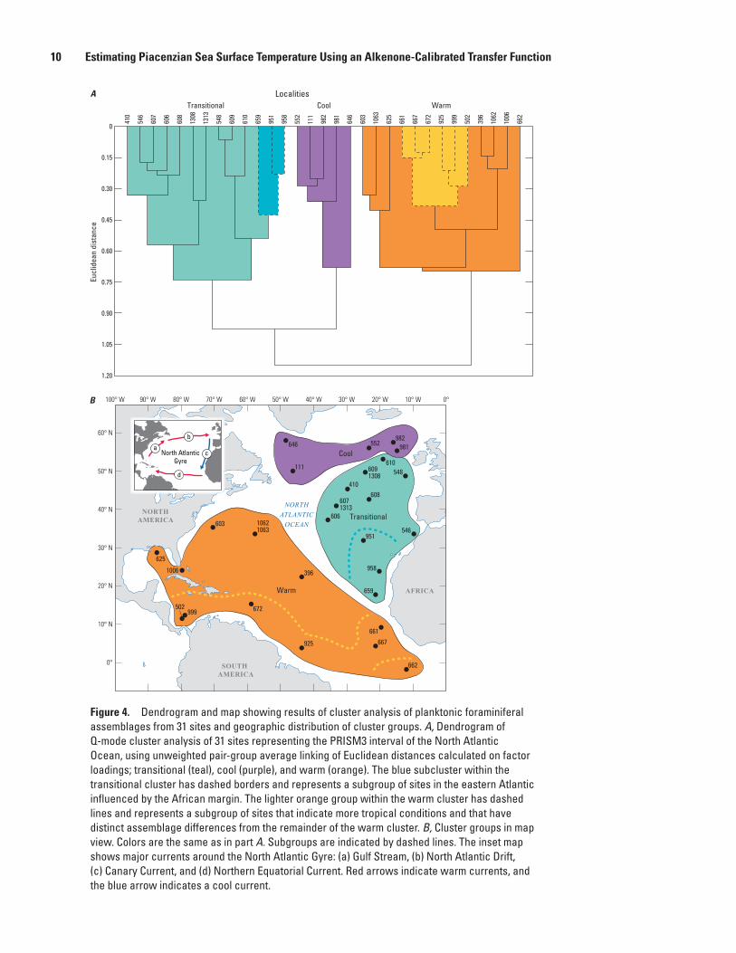
To aid interpretation, factor loadings were clustered by using an unweighted pair group algorithm (UPGMA), and the cluster groups were mapped geographically (fig. 4). Three main groups of samples are defined that are, as expected, simi-lar to Factors 1–3 (fig. 4). Samples in the low latitudes have assemblages coinciding with the warm factor. A subgroup can be distinguished along its southern margin tracing the southern limb of the North Atlantic Gyre and represents the warmest conditions (fig. 4). The other sites within this group are located along the general path of the Gulf Stream or in more subtropi-cal regions of the North Atlantic Gyre.

Sites belonging to the cool group defined by cluster anal-ysis are the same as those showing high loadings on Factor 3 (figs. 3, 4). A third group of sites is defined by the cluster analysis and occupies the eastern and northeastern region of the North Atlantic. This group extends beyond the region

−0.15−0.15

0

0.15

0.30

0.45

0.60

0.75

0.90

1.05

0 0.15 0.30 0.45 0.60 0.75 0.90

Fact

or 2

Factor 1

Warm

Cool

Transitional

502

546

552

603

606

609610

659

396

410

607

608

625

646

662

672925

951958

981982

9991062

1063

1308

1313

111

661

1006

667

548

Figure 2. Graph of results of factor analysis of Piacenzian planktonic foraminiferal assemblages showing sample loadings on Factor 1 and Factor 2 (table 2). Numbers by plotted points identify core sites where samples yielding the assemblages were obtained (table 1). Three groups of site numbers that are defined by shading and labeled “Warm,” “Transitional,” and “Cool” indicate sources of sample assemblages having affinities for warm, transitional, or cool water.

Results 9

Den

togl

obig

erin

a al

tispi

raG

lobi

gerin

a bu

lloid

esG

lobi

gerin

a fa

lcon

ensis

Glo

bige

rina

woo

diG

lobi

gerin

ella

aeq

uila

tera

lisG

lobi

gerin

ita g

lutin

ata

Glo

bige

rinoi

des o

bliq

uus

Glo

bige

rinoi

des r

uber

Glo

bige

rinoi

des s

accu

lifer

Glo

boro

talia

cra

ssaf

orm

isG

lobo

rota

lia h

irsut

aG

lobo

rota

lia m

enar

dii

Glo

boro

talia

pun

ctic

ulat

aG

lobo

rota

lia sc

itula

Neo

glob

oqua

drin

a ac

osta

ensis

Neo

glob

oqua

drin

a at

lant

ica

(d)

Neo

glob

oqua

drin

a at

lant

ica

(s)

Neo

glob

oqua

drin

a hu

mer

osa

Neo

glob

oqua

drin

a in

com

pta

Neo

glob

oqua

drin

a pa

chyd

erm

aO

rbul

ina

univ

ersa

Spha

eroi

dine

llops

is se

min

ulin

aTu

rbor

otal

ita q

uinq

uelo

ba

Fact

or 4

(5.1

%)

Fact

or 5

(3.2

%)

* *

**

*

Fact

or s

core

Fact

or 1

Tran

sitio

nal (

49.4

%)

Fact

or 2

War

m (2

1.7%

)Fa

ctor

3Co

ol (8

.7%

)

−1.5−1.0−0.5

00.51.01.5

2.5

2.0

−0.5

0

0.5

1.01.52.0

3.0

2.5

−1.0

0

1.0

2.0

3.0

4.0

5.0

−1.0−0.5

00.51.01.52.02.53.0

−1.0

−1.5

−0.5

0

0.5

1.01.5

2.02.5

Figu

re 3

. Gr

aphi

c re

pres

enta

tion

of th

e as

sem

blag

e de

scrip

tion

mat

rix s

how

ing

how

fora

min

ifera

l spe

cies

sco

re o

n fiv

e fa

ctor

s an

d pe

rcen

tage

of i

nfor

mat

ion

expl

aine

d.

Colo

r cod

ing

for t

rans

ition

al, w

arm

, and

coo

l fac

tors

as

in fi

gure

2; F

acto

r 4, g

reen

; Fac

tor 5

, gra

y. A

ster

isks

adj

acen

t to

bars

in th

e gr

aph

for F

acto

r 4 in

dica

te s

peci

es

cons

ider

ed to

be

ther

moc

line

dwel

lers

.


111

396

410

6071313

608

625

646

662

672

925

951

958

981982

999

1006

6091308

603606

610

659

661

667

548

552

502

54610621063

B

Warm

Cool

Transitional

SOUTH AMERICA

NORTHATLANTIC

OCEAN

NORTHAMERICA

AFRICA

North AtlanticGyre

a

d

b

c

100° W 90° W 80° W 70° W 60° W 50° W 40° W 30° W 20° W 10° W 0°

60° N

40° N

50° N

30° N

20° N

10° N

0°

0

0.15

0.30

0.45

0.60

0.75

0.90

1.05

1.20

Eucl

idea

n di

stan

ce

410

546

607

606

608

1308

1313

548

609

610

659

951

958

552

111

982

981

646

603

1063

625

661

667

672

925

999

502

396

1062

1006

662

ATransitional Cool Warm

Localities

Figure 4. Dendrogram and map showing results of cluster analysis of planktonic foraminiferal assemblages from 31 sites and geographic distribution of cluster groups. A, Dendrogram of Q-mode cluster analysis of 31 sites representing the PRISM3 interval of the North Atlantic Ocean, using unweighted pair-group average linking of Euclidean distances calculated on factor loadings; transitional (teal), cool (purple), and warm (orange). The blue subcluster within the transitional cluster has dashed borders and represents a subgroup of sites in the eastern Atlantic influenced by the African margin. The lighter orange group within the warm cluster has dashed lines and represents a subgroup of sites that indicate more tropical conditions and that have distinct assemblage differences from the remainder of the warm cluster. B, Cluster groups in map view. Colors are the same as in part A. Subgroups are indicated by dashed lines. The inset map shows major currents around the North Atlantic Gyre: (a) Gulf Stream, (b) North Atlantic Drift, (c) Canary Current, and (d) Northern Equatorial Current. Red arrows indicate warm currents, and the blue arrow indicates a cool current.

Discussion 11

where the transitional factor is most expressed and includes sites with a cool influence in the north and a warm influence in the south. Within this group, cluster analysis distinguishes a subgroup of sites heavily influenced by the Canary Current and sedimentation along the African margin (fig. 4).

Paleotemperature Equation

Multiple regression was used to write an equation relat-ing the five factors (f1 – f5) to mean annual SST derived using the U 37 K ′ index. The coefficient of determination (R2) for the equation is 0.87, and the root mean square (RMS) error is ±1.38 °C.

SST = −0.15( f1) + 11.3 ( f2) − 2.62( f3) + 4.04( f4) + 4.74( f5) + 17.24

This equation is constrained between ~17 and 29 °C.

Comparison of U 37 K ′ SST estimates and faunal SST estimates derived using the equation above, for 17 localities where we have both, show residuals less than 2 °C and do not exhibit any obvious latitudinal trends. Eleven of the 17 sites show alkenone estimates higher than faunal estimates.

This equation was applied to factor loadings from the 14 sites without alkenone records to estimate SST for those samples (table 1). Figure 5 shows the spatial distribution of SST estimates based upon alkenones and the transformed faunal data.

Discussion

Use of New Transfer Function

The assumption of stationarity, that Piacenzian and modern individuals of the same species have similar environmental preferences, has plagued pre-Quaternary paleotemperature reconstructions based on fossil assemblage data calibrated to modern coretop assemblage data. Kucera and Schönfeld (2007) cautioned that the nature of the modern foraminiferal fauna is a product of the most recent extinctions and diversification. Therefore, environmental proxies based on assemblages should not be interpreted quantitatively in sediments older than the late Pliocene. One solution to this problem is to disregard the mod-ern faunal preferences and directly calibrate Piacenzian taxa to

Piacenzian temperatures. The extensive Piacenzian faunal cen-sus datasets and paired Piacenzian U 37 K ′ SST values allow for the development of a factor analytic transfer function ideally suited to provide SST estimates at sites lacking alkenone analyses. The combination of SST estimates derived from alkenone analyses and the new transfer function provides a reconstruction of mean PRISM3 interval (3.264–3.025 Ma) SST in the North Atlantic with improved spatial resolution (fig. 5).

North Atlantic Sea Surface Temperature

Dowsett and others (2019) showed the North Atlantic latitudinal surface temperature gradient, calculated using U 37 K ′ SST estimates confined to MIS KM5c, to be essentially the same as that originally reconstructed using multiple tempera-ture proxies and a temporally more broad, less constrained time slab (Dowsett and others, 1992). The spatial pattern of alkenone SST estimates and those from the new transfer func-tion also show good agreement (fig. 5). These estimates, based upon an independent calibration, confirm the pattern of spatial SST variability documented in previous Pliocene reconstruc-tions of the North Atlantic (Dowsett, 2007; Dowsett and oth-ers, 1992, 2010, 2012). This expanded set of comparison data will be useful for future data-model comparison.

The SST estimates from ODP Sites 981 and 982, located close to each other (fig. 5), differ by ~2 °C (15.7 °C and 17.6 °C, respectively). The Site 982 record is based on alkenones (Lawrence and others, 2009; Dowsett and others, 2017), whereas the estimates from Site 981 are derived from faunal assemblages and the transfer function presented here. To better understand why these estimates are different, we first applied the transfer function to the Site 982 faunal assemblage. That analysis provides an SST estimate only 0.5 °C cooler than the alkenone estimate. This estimate and the high com-munalities for both Sites 981 and 982 (table 1) suggest that transfer function performance is robust. The Site 982 samples were collected from the entire PRISM3 stratigraphic interval, whereas the Site 981 data are restricted to an interval of cool-ing correlated to the δ18O enrichment associated with the MIS M1—MIS KM6 transition. The primary difference between the mean assemblages at the two sites is a higher abundance of N. atlantica (s) at Site 981. This increases the strength of the cool assemblage, and, in turn, results in a colder transfer function estimate (table 1). For comparison, applying the transfer function to the same cool interval at Site 982 results in an estimated SST of 16.0 °C, only 0.3 °C warmer than the estimate at Site 981.

(5)


0 4 8 12 16 20 24 28 32

Mean sea surface temperature, in degrees Celsius

Alkenone Transfer function

EXPLANATION

100° W 90° W 80° W 70° W 60° W 50° W 40° W 30° W 20° W 10° W 0°

60° N

40° N

50° N

30° N

20° N

10° N

0°

111

396

410

608

625

646

662

672

925

951

958

981982

999

1006

603606

610

659

661

667

548

552

546

502

6071313

6091308

10621063

SOUTH AMERICA

NORTHATLANTIC OCEAN

NORTHAMERICA

AFRICA

Figure 5. Map showing PRISM3 mean sea surface temperatures (SST) for 31 sites in the North Atlantic Ocean. Symbols with solid borders are U 37 K ′ (alkenone) SST estimates. Symbols with dashed borders are estimates derived by using a new transfer function.

References Cited 13

Summary and ConclusionsPrevious faunal transfer functions relied upon calibration

of modern taxa to temperature or to another oceanographic variable. For Pliocene applications, fossil faunas were, out of necessity, assessed in terms of the modern model to estimate paleoenvironmental conditions. Thus, to use faunal techniques to estimate Pliocene temperature, stationarity was conse-quently assumed over the last 3 million years. If we instead assume stationarity of environmental tolerances only over a narrow interval of time, and calibrate directly to that same interval, our assumptions become more likely, and precise chronology within the interval becomes less important.

We explore another way to estimate Pliocene paleoen-vironments without assuming environmental stationarity. We use independent alkenone-based mean paleotempera-ture estimates to directly calibrate mean abundance data of Pliocene Foraminifera from within the PRISM3 time slab (3.264 Ma–3.025 Ma). Initial results are encouraging in that Pliocene faunal census data, converted to mean annual SST estimates, fit well with alkenone-based estimates. This meth-odology allows utilization of the large amount of PRISM fau-nal census data in order to expand spatial SST reconstructions.

The availability of U 37 K ′ SST estimates on an increasing number of Pliocene sequences, combined with the availabil-ity of taxonomically consistent global Pliocene planktonic foraminiferal census data, provides a unique opportunity to assess the assumption of stationarity, to help evaluate preferences assumed for now extinct taxa, and to estimate paleotemperatures.

It is important to remember that attempts at reconstruct-ing a single environmental variable, like mean annual SST, are oversimplifications of complex and variable interactions between individuals and the n-dimensional hypervolume or niche (Hutchinson, 1957) within which a species of planktonic foraminifer can survive. While temperature is a first-order control on foraminifer abundance and distribution, many other factors (such as productivity, salinity, and nutrients) also play a role.

Advances in chronology allow for more precise correla-tions between sedimentary archives, but the fundamental fau-nal assemblage-based signals preserved in sedimentary records are still limited by the degree of time averaging inherent in the signal and added to the signal by postdepositional processes (such as sediment mixing due to bioturbation). During life, Foraminifera respond to a range of sub-annual processes that result in the discontinuous and seasonal rain of material to the sea floor. Depositional and postdepositional processes serve as a low-pass filter on the already time-averaged environmental signal embedded in foraminiferal assemblages. Our decision to degrade the temporal signal further, by averaging samples within the ~240 kyr PRISM3 interval, filters out potentially important responses to high-frequency ecological and envi-ronmental changes and places constraints on the resolution of

paleoenvironmental reconstruction. Nevertheless, comparisons of these SST values with previous data show similar patterns of warmth for the Piacenzian.

References Cited

Badger, M.P.S., Schmidt, D.N., Mackensen, A., and Pancost, R.D., 2013, High-resolution alkenone palaeobarom-etry indicates relatively stable pCO2 during the Pliocene (3.3–2.8 Ma): Philosophical Transactions of the Royal Society, A, v. 371, no. 2001, article 20130094, 16 p., accessed March 15, 2014, at https://doi.org/ 10.1098/ rsta.2013.0094.

Berggren, W.A., 1973, The Pliocene time scale—Calibration of planktonic foraminiferal and calcareous nannoplankton zones: Nature, v. 243, no. 5407, p. 391–397.

Blow, W.H., 1969, Late middle Eocene to Recent planktonic foraminiferal biostratigraphy, in Brönnimann, P., and Renz, H.H., eds., Proceedings of the First International Conference on Planktonic Microfossils, Geneva, 1967: Leiden, E.J. Brill, v. 1, p. 199–422.

CLIMAP Project Members, 1984, The last interglacial ocean: Quaternary Research, v. 21, no. 2, p. 123–224.

Cline, R.M., and Hays, J.D., eds., 1976, Investigation of late Quaternary paleoceanography and paleoclimatology: Geological Society of America Memoir 145, 464 p.

Dowsett, H.J., 2007, The PRISM palaeoclimate reconstruc-tion and Pliocene sea-surface temperature, in Williams, M., Haywood, A.M., Gregory, F.J., and Schmidt, D.N., eds., Deep-time perspectives on climate change—Marrying the signal from computer models and bio-logical proxies: London, Geological Society of London; Micropalaeontological Society Special Publication, [no. 2], p. 459–480.

Dowsett, H.J., Cronin, T.M., Poore, R.Z., Thompson, R.S., Whatley, R.C., and Wood, A.M., 1992, Micropaleontological evidence for increased meridi-onal heat transport in the North Atlantic Ocean during the Pliocene: Science, v. 258, no. 5085, p. 1133–1135.

Dowsett, H.[J.], Dolan, A., Rowley, D., Moucha, R., Forte, A.M., Mitrovica, J.X., Pound, M., Salzmann, U., Robinson, M., Chandler, M., Foley, K., and Haywood, A., 2016, The PRISM4 (mid-Piacenzian) paleoenvironmental recon-struction: Climate of the Past, v. 12, no. 7, p. 1519–1538, accessed June 7, 2019, at https://doi.org/ 10.5194/ cp- 12- 1519- 2016.

https://doi.org/10.1098/rsta.2013.0094

https://doi.org/10.1098/rsta.2013.0094

https://doi.org/10.5194/cp-12-1519-2016

https://doi.org/10.5194/cp-12-1519-2016


Dowsett, H.J., Foley, K.M., Robinson, M.M., and Herbert, T.D., 2017, PRISM late Pliocene (Piacenzian) alkenone-derived SST data: U.S. Geological Survey data release, accessed June 7, 2019, at https://doi.org/ 10.5066/ F7959G1S.

Dowsett, H.J., and Poore, R.Z., 1990, A new planktic fora-minifer transfer function for estimating Pliocene–Holocene paleoceanographic conditions in the North Atlantic: Marine Micropaleontology, v. 16, nos. 1–2, p. 1–23, accessed August 11, 1993, at https://doi.org/ 10.1016/ 0377- 8398(90)90026- I.

Dowsett, H.J., and Robinson, M.M., 2006, Stratigraphic framework for Pliocene paleoclimate reconstruction—The correlation conundrum: Stratigraphy, v. 3, no. 1, p. 53–64.

Dowsett, H.J., and Robinson, M.M., 2007, Mid-Pliocene planktic foraminifer assemblage of the North Atlantic Ocean: Micropaleontology, v. 53, nos. 1–2, p. 105–126.

Dowsett, H.[J.], Robinson, M., and Foley, K., 2015, A global planktic foraminifer census data set for the Pliocene ocean: Scientific Data, v. 2, article 150076, 6 p., accessed December 9, 2018, at https://doi.org/ 10.1038/ sdata.2015.76.

Dowsett, H.J., Robinson, M.M., Foley, K.M., Herbert, T.D., Otto-Bliesner, B.L., and Spivey, W., 2019, The mid-Piacenzian of the North Atlantic Ocean: Stratigraphy, v. 16, no. 3, p. 119–144, accessed January 28, 2020, at https://doi.org/ 10.29041/ strat.16.3.119- 144.

Dowsett, H.J., Robinson, M.M., Haywood, A.M., Hill, D.J., Dolan, A.M., Stoll, D.K., Chan, W.-L., Abe-Ouchi, A., Chandler, M.A., Rosenbloom, N.A., Otto-Bliesner, B.L., Bragg, F.J., Lunt, D.J., Foley, K.M., and Riesselman, C.R., 2012, Assessing confidence in Pliocene sea surface tempera-tures to evaluate predictive models: Nature Climate Change, v. 2, no. 5, p. 365–371.

Dowsett, H.[J.], Robinson, M., Haywood, A.M., Salzmann, U., Hill, D., Sohl, L.E., Chandler, M., Williams, M., Foley, K., and Stoll, D.K., 2010, The PRISM3D paleoenvironmental reconstruction: Stratigraphy, v. 7, nos. 2–3, p. 123–139.

Herbert, T.D., Peterson, L.C., Lawrence, K.T., and Liu, Z., 2010, Tropical ocean temperatures over the past 3.5 million years: Science, v. 328, no. 5985, p. 1530–1534, accessed March 15, 2019, at https://doi.org/ 10.1126/ science.1185435.

Herbert, T.D., Yasuda, M., and Burnett, C., 1995, Glacial-interglacial sea-surface temperature record inferred from alkenone unsaturation indices, site 893, Santa Barbara Basin: Proceedings of the Ocean Drilling Program, Scientific Results, v. 146 (pt. 2), p. 257–264.

Hutchinson, G.E., 1957, Concluding remarks: Cold Spring Harbor Symposia on Quantitative Biology, v. 22, p. 415–427, accessed March 18, 2019, at https://doi.org/ 10.1101/ SQB.1957.022.01.039.

Hutson, W.H., 1980, The Agulhas Current during the late Pleistocene—Analysis of modern faunal analogs: Science, v. 207, no. 4426, p. 64–66, accessed March 18, 2019, at https://doi.org/ 10.1126/ science.207.4426.64.

Imbrie, J., and Kipp, N.G., 1971, A new micropaleontological method for quantitative paleoclimatology—Application to a late Pleistocene Caribbean core, in Turekian, K.K., ed., The late Cenozoic glacial ages: New Haven, Conn., Yale University Press, p. 71–181.

Keigwin, L.D., 1976, Late Cenozoic planktonic foraminiferal biostratigraphy and paleoceanography of the Panama Basin: Micropaleontology, v. 22, no. 4, p. 419–442.

Khélifi, N., Sarnthein, M., and Naafs, B.D.A., 2012, Technical note—Late Pliocene age control and composite depths at ODP site 982, revisited: Climate of the Past, v. 8, no. 1, p. 79–87.

Klovan, J.E., and Imbrie, J., 1971, An algorithm and FORTRAN-IV program for large-scale Q-mode factor anal-ysis and calculation of factor scores: Mathematical Geology, v. 3, no. 1, p. 61–77. [Also available at https://doi.org/ 10.1007/ BF02047433.]

Kucera, M., and Schönfeld, J., 2007, The origin of modern oceanic foraminiferal faunas and Neogene climate change, in Williams, M., Haywood, A.M., Gregory, F.J., and Schmidt, D.N., eds., Deep-time perspectives on climate change—Marrying the signal from computer models and biological proxies: London, Geological Society of London; Micropalaeontological Society Special Publication, [no. 2], p. 409–425.

Lawrence, K.T., Herbert, T.D., Brown, C.M., Raymo, M.E., and Haywood, A.M., 2009, High-amplitude variations in North Atlantic sea surface temperature during the early Pliocene warm period: Paleoceanography, v. 24, no. 2, article PA2218, 15 p., accessed March 15, 2018, at https://doi.org/ 10.1029/ 2008pa001669.

Lawrence, K.T., Herbert, T.D., Dekens, P.S., and Ravelo, A.C., 2007, The application of the alkenone organic proxy to the study of Plio-Pleistocene climate, in Williams, M., Haywood, A.M., Gregory, F.J., and Schmidt, D.N., eds., Deep-time perspectives on climate change—Marrying the signal from computer models and bio-logical proxies: London, Geological Society of London; Micropalaeontological Society Special Publication, [no. 2], p. 539–562.



https://doi.org/10.1016/0377-8398(90)90026-I

https://doi.org/10.1016/0377-8398(90)90026-I

https://doi.org/10.1038/sdata.2015.76

https://doi.org/10.29041/strat.16.3.119-144

https://doi.org/10.1126/science.1185435

https://doi.org/10.1101/SQB.1957.022.01.039

https://doi.org/10.1101/SQB.1957.022.01.039

https://doi.org/10.1126/science.207.4426.64

https://doi.org/10.1007/BF02047433

https://doi.org/10.1007/BF02047433

https://doi.org/10.1029/2008pa001669

References Cited 15

Lawrence, K.T., Sosdian, S., White, H.E., and Rosenthal, Y., 2010, North Atlantic climate evolution through the Plio-Pleistocene climate transitions: Earth and Planetary Science Letters, v. 300, nos. 3–4, p. 329–342, accessed March 15, 2019, at https://doi.org/ doi:10.1016/ j.epsl.2010.10.013.

Lisiecki, L.E., and Raymo, M.E., 2005, A Pliocene‐Pleistocene stack of 57 globally distributed benthic δ18O records: Paleoceanography, v. 20, no. 1, article PA1003, 17 p., accessed October 14, 2015, at https://doi.org/ 10.1029/ 2004PA001071.

Malmgren, B.A., Kucera, M., Nyberg, J., and Waelbroeck, C., 2001, Comparison of statistical and artificial neural network techniques for estimating past sea surface temperatures from planktonic foraminifer census data: Paleoceanography, v. 16, no. 5, p. 520–530. [Also available at https://doi.org/ 10.1029/ 2000PA000562.]

Malmgren, B.A., and Nordlund, U., 1997, Application of artificial neural networks to paleoceanographic data: Palaeogeography, Palaeoclimatology, Palaeoecology, v. 136, nos. 1–4, p. 359–373.

Müller, P.J., Kirst, G., Ruhland, G., von Storch, I., and Rosell-Melé, A., 1998, Calibration of the alkenone paleotempera-ture index U37

K′ based on core-tops from the eastern South Atlantic and the global ocean (60°N–60°S): Geochimica et Cosmochimica Acta, v. 62, no. 10, p. 1757–1772.

Naafs, B.D.A., Stein, R., Hefter, J., Khélifi, N., De Schepper, S., and Haug, G.H., 2010, Late Pliocene changes in the North Atlantic Current: Earth and Planetary Science Letters, v. 298, nos. 3–4, p. 434–442.

Ogg, J.G., Ogg, G.M., and Gradstein, F.M., 2016, A concise geologic time scale—2016: Amsterdam, Elsevier, 240 p.

Parker, F.L., 1962, Planktonic foraminiferal species in Pacific sediments: Micropaleontology, v. 8, no. 2, p. 219–254.

Parker, F.L., 1967, Late Tertiary biostratigraphy (plank-tonic Foraminifera) of tropical Indo-Pacific deep-sea cores: Bulletins of American Paleontology, v. 52, no. 235, p. 115–208.

Robinson, M.M., Dowsett, H.J., Dwyer, G.S., and Lawrence, K.T., 2008, Reevaluation of mid-Pliocene North Atlantic sea surface temperatures: Paleoceanography, v. 23, no. 3, article PA3213, 9 p., accessed October 7, 2012, at https://doi.org/ 10.1029/ 2008PA001608.

Robinson, M.M., Foley, K., Dowsett, H.J., and Spivey, W., 2019, A global planktic foraminifer census data set for the Pliocene ocean, addendum: National Oceanic and Atmospheric Administration, National Centers for Environmental Information [formerly National Climatic Data Center] website, accessed January 4, 2020, at https: //www.ncdc .noaa.gov/ paleo/ study/ 27310.

Sabaa, A.T., Sikes, E.L., Hayward, B.W., and Howard, W.R., 2004, Pliocene sea surface temperature changes in ODP site 1125, Chatham Rise, east of New Zealand: Marine Geology, v. 205, nos. 1–4, p. 113–125.

Thunell, R.C., 1979, Pliocene–Pleistocene paleotemperature and paleosalinity history of the Mediterranean Sea—Results from DSDP sites 125 and 132: Marine Micropaleontology, v. 4, p. 173–187.

https://doi.org/doi:10.1016/j.epsl.2010.10.013

https://doi.org/10.1029/2004PA001071

https://doi.org/10.1029/2004PA001071

https://doi.org/10.1029/2000PA000562

https://doi.org/10.1029/2000PA000562

https://doi.org/10.1029/2008PA001608

https://doi.org/10.1029/2008PA001608




Appendix 1. Species ListThe following list has names of planktonic foraminiferal

species for which abundance data were used in this study (table 1). Samples containing the species were obtained from 31 sites in the North Atlantic Ocean.

Dentoglobigerina altispira (Cushman & Jarvis, 1936)Globigerina bulloides d’Orbigny, 1826Globigerina falconensis Blow, 1959Globigerina woodi Jenkins, 1960Globigerinella aequilateralis (Brady, 1879)Globigerinita glutinata (Egger, 1893)Globigerinoides obliquus Bolli, 1957Globigerinoides ruber (d’Orbigny, 1839a)Globigerinoides sacculifer (Brady, 1877)Globorotalia crassaformis (Galloway & Wissler, 1927)Globorotalia hirsuta (d’Orbigny, 1839b)Globorotalia menardii (d’Orbigny in Parker, Jones &

Brady, 1865)Globorotalia puncticulata (Deshayes, 1832)Globorotalia scitula (Brady, 1882)Neogloboquadrina acostaensis (Blow, 1959)Neogloboquadrina atlantica (Berggren, 1972)1

Neogloboquadrina humerosa (Takayanagi & Saito, 1962)Neogloboquadrina incompta (Cifelli, 1961)Neogloboquadrina pachyderma (Ehrenberg, 1862)Orbulina universa d’Orbigny, 1839aSphaeroidinellopsis seminulina (Schwager, 1866)Turborotalita quinqueloba (Natland, 1938)

1For N. atlantica, we separated dextral (d) and sinistral (s) varieties into distinct counting categories as shown in table 1.

References CitedBerggren, W.A., 1972, Cenozoic biostratigraphy and paleobio-

geography of the North Atlantic: Initial Reports of the Deep Sea Drilling Project, v. 12, p. 965–1001, 13 pls.

Blow, W.H., 1959, Age, correlation and biostratigraphy of the upper Tocuyo (San Lorenzo) and Pozón Formations, eastern Falcón, Venezuela: Bulletins of American Paleontology, v. 39, no. 178, p. 67–252, 19 pls.

Bolli, H.M., 1957, Planktonic Foraminifera from the Oligocene–Miocene Cipero and Lengua Formations of Trinidad, B.W.I.: U.S. National Museum Bulletin 215, p. 97–123.

Brady, H.B., 1877, II.—Supplementary note on the Foraminifera of the Chalk (?) of the New Britain Group: Geological Magazine (London), new ser., decade 2, v. 4, no. 12, p. 534–536.

Brady, H.B., 1879, Notes on some of the reticularian Rhizopoda of the “Challenger” Expedition—[part] I.—On new or little known arenaceous types: Quarterly Journal of Microscopical Science, v. 19, new series, no. 73, p. 20–63, 3 pls.

Brady, H.B., 1882, Report on the Foraminifera, in Tizard, [T.H.], and Murray, [J.], Exploration of the Faroe Channel during the summer of 1880, in H.M.’s [Her Majesty’s] hired ship “Knight Errant”: Proceedings of the Royal Society of Edinburgh, v. 11, no. 11, p. 708–717.

Cifelli, R., 1961, Globigerina incompta, a new species of pelagic Foraminifera from the North Atlantic: Contributions from the Cushman Foundation for Foraminiferal Research, v. 12, p. 83–86.

Cushman, J.A., and Jarvis, P.W., 1936, Three new Foraminifera from the Miocene Bowden Marl of Jamaica: Contributions from the Cushman Laboratory for Foraminiferal Research, v. 12, p. 3–5.

Appendix 1 17

Deshayes, G.P., 1832, Encyclopédie méthodique—Histoire naturelle des vers: Paris, v. 2, 594 p.

d’Orbigny, A.D., 1826, Tableau méthodique de la classe des Céphalopodes: Annales des Sciences Naturelles, v. 7, p. 245–314.

d’Orbigny, A.D., 1839a, Foraminifères, v. 8 of Sagra, R. de la, ed., Histoire physique, politique et naturelle de l’ile de Cuba: Paris, A. Bertrand, 224 p.

d’Orbigny, A.D., 1839b, Foraminifères des Îles Canaries: Histoire naturelle des Iles Canaries, v. 2, no. 2, p. 120–146. [Also available at https://archive.org/ stream/ Histoir enaturelII Webb#page/ n375/ .]

Egger, J.G., 1893, Foraminiferen aus Meeresgrundproben, gelothet von 1874 bis 1876 von S. M. Sch. Gazelle: Abhandlungen der Mathematisch-Physikalischen Classe der Königlich Bayerischen Akademie der Wissenschaften, v. 18, section 2, p. 193–457.

Ehrenberg, C.G., 1862, Über die Tiefgrund-Verhältnissse des Ozeans am Eingange der Davisstrasse und bei Island: Monatsberichte der Königlichen Preussische Akademie der Wissenschaften zu Berlin, p. 275–315.

Galloway, J.J., and Wissler, S.G., 1927, Pleistocene Foraminifera from the Lomita Quarry, Palos Verdes Hills, California: Journal of Paleontology, v. 1, no. 1, p. 35–87.

Jenkins, D.G., 1960, Planktonic Foraminifera from the Lakes Entrance oil shaft, Victoria, Australia: Micropaleontology, v. 6, no. 4, p. 345–371.

Natland, M.L., 1938, New species of Foraminifera from off the west coast of North America and from the later Tertiary of the Los Angeles Basin: Bulletin of the Scripps Institution of Oceanography, Technical Series, v. 4, no. 5, p. 137–163.

Parker, W.K., Jones, T.R., and Brady, H.B., 1865, IV.—On the nomenclature of the Foraminifera; Part X. (continued).—The species, enumerated by d’Orbigny in the “Annales des Sciences Naturelles,” vol. vii, 1826; III. The species illus-trated by models: Annals and Magazine of Natural History, ser. 3, v. 16, no. 91, p. 15–41.

Schwager, C., 1866, Fossile Foraminiferen von Kar Nikobar—Reise der Oesterreichischen Fregatte Novara um die Erde in den Jahren 1857, 1858, 1859 unter den Befehlen des Commodore B. von Wüllerstorf-Urbair, Geologischer Theil, Geologische Beobachtung no. 2: Palaeontologische Mittheilung 2, p. 187–268.

Takayanagi, Y., and Saito, T., 1962, Planktonic Foraminifera from the Nobori Formation, Shikoku, Japan: Science Reports of the Tohoku University Second Series (Geology), v. 5, p. 67–105.

https://archive.org/stream/HistoirenaturelIIWebb#page/n375/

https://archive.org/stream/HistoirenaturelIIWebb#page/n375/

Dowsett and others—

Estimating Piacenzian Sea Surface Tem

perature Using an A

lkenone-Calibrated Transfer Function—SIR 2021–5051

ISSN 2328-0328 (online)https://doi.org/ 10.3133/ sir20215051

https://doi.org/10.3133/sir20215051

estimating piacenzian sea surface temperature using an

Documents